Lateral-Torsional-Axial coupled vibration for a geared system

1

Lateral-Torsional-Axial coupled vibration for a geared system

In the vibration study of a single rotor system, the lateral, torsional, and axial vibrations are

typically decoupled and can be studied separately in general. However, for a geared rotor system

with multiple rotors, the lateral, torsional, and axial vibration are coupled through the gear mesh

and/or rider ring (sometimes called thrust collar ring), as illustrated in Figure 1. The rider ring is

commonly used in turbomachinery applications, such compressors and expanders, to transfer the

thrust load from high speed pinions to the low speed gear to reduce the mechanical friction loss

and eliminate thrust bearings in the high speed pinions, as shown in Figure 2. The rider ring is

more commonly used in high speed and low power small machines where the mechanical

frictional power loss is critical to the entire machine and the cost is also competitive in the

market.

Figure 1 Geared system with rider ring

2

Figure 2 Rider ring for thrust balance

Consider a gear-paired system, as shown in Figure 3, gear 1 is used as a reference gear where the

gear 2 angular position, , is specified with respect to the gear 1. Gear 1 can be either a driving or

driven shaft and rotates CCW or CW. The (X,Y,Z) coordinate system is a fixed Cartesian

coordinate system with Z axis in line with the spinning axis and X and Y in the transverse

directions perpendicular to the Z axis, following the right hand rule. The motion for each finite

element station along the rotor (including the gear center) is described by 6 degrees-of-freedom:

three (3) translational displacements (x,y,z) along (X,Y,Z) axes and three (3) rotational

displacements ( zyx ,, ) about (X,Y,Z) axes. For lateral vibration, the motion of each finite

element station is described by two translational displacements (x,y) in the X and Y directions

respectively, and two rotational (angular) displacements (x,y) about the X and Y axes

respectively. For torsional vibration, the motion of each finite element station is described by a

rotational displacement ( z ) about the spinning axis (Z). For axial vibration, the motion of each

finite element station is described by a translational displacement (z) along the spinning axis (Z).

3

Therefore, the motions at a typical finite element station are described by the following

displacement vectors:

Complete motion: T

(6X1) , , , , , x y zx y z q (1a)

Lateral vibration: , , , T

L x yx y q (1b)

Torsional vibration: T zq (1c)

Axial vibration: A zq (1d)

Figure 3 A typical gear set

4

Note that the spinning direction of the rotor is commonly defined as CCW along the positive Z

axis (+Z) for a single rotor system. However, for a geared multiple rotor system, some rotors will

rotate CW in the negative Z direction (-Z). Therefore, caution must be taken when defining the

forward and backward precessions of the lateral orbit motion. The detailed explanation of the

orbit motion has been documented in Chen and Gunter (2005), some highlights and cautions for

the geared system are addressed here.

The lateral rotor motion at each finite element station is either forward or backward precession in

relation to the direction of rotation (spin) of the rotor and not the direction of the Z axis, as

shown in Figure 4. The whirling motion is defined as a forward precession if it is whirling in the

same direction as the rotor spinning direction, and as a backward precession if it is whirling

opposite to the rotor spinning direction. A straight line motion is a degeneration of a whirling

orbit and a transition between the forward and backward precessions without the whirling

motion.

Figure 4 Whirling orbits

5

The direction of precession, or a whirling direction, of a lateral vibration orbit is defined by the

rate of precession angle in the (X,Y) plane. The precessional angle is defined as:

)(

)(arctan)(

tx

tyt (2)

The direction of precession (whirling) is determined by the rate of precessional angle

sign (3)

When is a positive value (CCW) and the rotor is spinning in the positive Z direction (CCW),

the orbit motion is a forward whirl (precession). When is a negative value (CW) and the rotor

is spinning in the positive Z direction (CCW), the orbit motion is a backward whirl (precession).

When is zero the orbit motion degenerates into a straight-line path without whirling.

However, when the rotor is spinning in the negative Z direction (CW), then a positive (CCW)

indicates a backward whirl and a negative (CW) indicates a forward whirl. For a single rotor

system, this confusion can be avoided by modeling the rotor with positive Z is the spinning

direction. For a multiple rotor geared system, the spinning direction of a rotor can be either in

the positive or negative Z axis. Therefore, it is convenient to define the rotor speed Ω as a vector

with direction. That is, if the rotor is spinning in the positive Z direction, the rotor rotational

speed Ω is positive and vice versa. Then the forward and backward whirl is defined by the

product of and :

Forward whirl (precession): > 0 is positivesign (4a)

Backward whirl (precession): < 0 is negativesign (4b)

Straight line motion: = 0 (4c)

Another caution is that almost all the calculated bearing coefficients, including the so-called

aerodynamic cross-coupling terms , xy yxk Q k Q where Q is a positive value, are obtained

with the assumption that the spinning direction is in the positive Z direction (CCW). With the

opposite spinning direction, i.e., spinning in the (-Z) direction, all the cross-coupled stiffness and

damping coefficients (kxy, kyx, ,x y

k k , cxy, cyx, ,x y

c c ) must change sign to accommodate the

negative spinning direction. Since the shaft (rotor) properties is isotropic for a circular cross-

section, therefore the rotor governing equation and related matrices are not affected by this

spinning direction, with the exception on the sign of the gyroscopic matrix and related forcing

vectors.

For a purely torsional vibration, it is commonly describe the torsional vibration rotational

displacement *

z in the same direction as the spinning direction. For a geared system, this

could lead to some confusions since the directions of rotor rotation are opposite for a mating gear

set. In this context, for consistency, we will use the definition in Eq. (1) for the rotor vibration

6

displacements. That is, the torsional displacement z is defined along the positive Z axis,

regardless the spinning direction. Therefore for a positive Ω, *

z z , and for a negative Ω, *

z z .

In summary, when analyzing the geared rotor system and the motion at each finite element

station is defined in Eq, (1), then the following cautions must be taken:

1. Treat the rotor rotational speed Ω as a vector, positive if it rotates in the positive Z direction

(CCW for a right hand ruled Cartesian coordinate system as used in Eq, (1)) and negative if it

rotates in the negative Z direction (CW). This will take care of the gyroscopic matrix and related

forcing function involved rotational speed.

2. Change the cross-coupled bearing stiffness and damping coefficients if necessary when the

rotor speed is negative, since almost all the bearing coefficients are obtained by assuming the

rotor speed is positive in the positive Z direction. This is particularly important when performing

the stability analysis since cross-coupled stiffness coefficients, including the aerodynamic cross-

coupling term, significantly affect the system stability.

3. When viewing the results for lateral motion, the direction of whirling needs to take into

account the rotor speed. That is, the forward and backward whirl is defined by the product of

and , not just as used for a single rotor system.

7

Example 1: A dual rotor system

A dual rotor system, as shown in Figure 1-1, is utilized here to demonstrate the effects of rotor

direction of rotation on the system dynamics. For multiple rotor systems, if all the shafts are in

the same axis and connected through couplings with the same rotational speed and direction of

rotation, then they can really be treated or modeled as a single rotor system and all the

discussions on the single rotor system are valid. However, for system as demonstrated in this

dual rotor system and geared systems (which will be discussed later), the rotors are having their

own rotational speed and direction of rotation. Then, the results will not be easily comprehended

and deserve some discussions. This dual rotor system has been presented by many publications

by Nelson, etc. and the system details are analyzed and documented in Chen & Gunter (2005)

with the same direction of rotation. Since rotors are supported by isotropic bearings with

constant stiffness and damping coefficients, the effects of rotational speed (magnitude and

direction) on the system dynamics are discussed here. Only the lateral vibrations are considered

and torsional and axial vibrations are neglected in this example.

Figure 1-1 Dual rotor system

Case 1: 2 11.5 , Ω1: CCW and Ω2: CCW

Let us review our previous discussion in Chen & Gunter with 2 11.5 . That is, the rotor 2

rotates in the same direction of rotation with rotor 1 in a speed ratio of 1.5. The speed

relationship is entered in the Shaft Elements tab. A positive value indicates a CCW rotation and

a negative value indicates a CW rotation. To display the direction of rotation, the check box in

the Model Graphic Settings must be checked.

8

9

Assuming the both rotors rotate CCW in the positive Z direction in this first case. Figure 1-2,

whirl speed map, shows the first 4 system damped natural frequencies verse the rotor speeds with

the synchronous excitation lines overlapped in the maps. It is noted that these two graphs are

identical with the exception of the scale in the X-axis (speed axis), where one labeled with the

rotor 1 speed and the other labeled with rotor 2 speed. These four frequencies (modes) are

labeled as ( 1 2 3 4, , , ) for identification purpose. Also noted that in addition to the using of

the forward and backward precession labels (F, B), the (CCW+) and (CW-) are also used to

represent the direction of whirling of the mode. So, the first and third modes whirl in the CW (-

Z) direction and the second and fourth modes whirl in the CCW (+Z) direction. Since both

rotors rotate CCW (+Z) direction, so, modes 1 and 3 are backward precession modes for both

rotors, and modes 2 and 4 are forward precession modes for both rotors. At zero speed, modes

(1, 2) and (3, 4) are essentially the planar modes with the same frequency, one in X direction

and the other in Y direction, and they form two circular whirling modes, one forward and the

other backward, due to gyroscopic effects as the speed increases in this example. The

gyroscopic effect stiffens the forward precession modes (increases the associated frequencies)

and softens the backward precession modes (decreases the associated frequencies).

Figure 1-2 Whirl speed map for 2 11.5

The associated mode shapes with whirling directions for the rotor speeds of

1 2, 10000,15000 rpm are shown in Figure 1-3. Again, the mode shapes for the first and

second modes are very similar and mode shapes for the third and fourth modes are very similar.

For the first and third modes, both rotors are whirling in the CW direction with a whirl frequency

of 5825 and 14189 cpm, respectively. For the second and fourth modes, both rotors are whirling

in the CCW direction with a whirl frequency of 8504 and 15260 cpm, respectively. Since both

rotors rotate CCW, therefore, the second and fourth modes are classified as the forward

precessional modes, and the first and third modes are referred to as the backward precessional

modes. For the isotropic systems, the mass unbalance excites the forward modes only.

Therefore, the critical speeds are the intersections of frequency curves of modes 2 and 4 and the

excitation lines in the whirl speed map.

10

Figure 1-3 Precessional mode shapes at speed of Ω1=10000, Ω2=15000 rpm

After knowing the mode precessional direction, we can go back to examine the whirl speed maps

and to identify the critical speeds due to shaft mass unbalance. The damped critical speeds are

the intersection points between the system natural frequencies and the synchronous excitation

line in the whirl speed map. The first two critical speeds due to rotor 1 mass unbalance occur at

rotor speeds of about (Ω1=8250, Ω2=12375 rpm) and (Ω1=15292, Ω2=22938 rpm) with the

whirling frequencies of 8250 and 15292 cpm, respectively. That is, the critical speeds due to

rotor 1 mass unbalance are identified by the excitation line with the spin(1)/whirl ratio of 1, i.e.,

( 1 1

, 2 1.5

). And the first two critical speeds due to rotor 2 mass unbalance occur at

rotor speeds of about (Ω1=5233, Ω2=7849 rpm) and (Ω1=10062, Ω2=15093 rpm) with the

whirling frequencies of 7849 and 15093 cpm, respectively. That is, the critical speeds due to

rotor 2 mass unbalance are identified by the spin(2)/whirl ratio of 1, i.e.,

( 2 1

, 1 1

0.666671.5

). Therefore, the first forward mode (2) will be excited by the

rotor 2 mass unbalance at rotor speed about (Ω1=5233, Ω2=7849 rpm) and again be excited by

the rotor 1 mass unbalance at rotor speed about (Ω1=8250, Ω2=12375 rpm) during the startup.

The second forward mode (4) will be excited by the rotor 2 mass unbalance at rotor speed about

(Ω1=10062, Ω2=15093 rpm) and again be excited by the rotor 1 mass unbalance at rotor speed

about (Ω1=15292, Ω2=22938 rpm) during the startup. Each forward mode is excited twice by

11

the mass unbalance during startup in this case, the first one is by rotor 2 mass unbalance due to

higher speed ratio and the other is by rotor 1 mass unbalance. The backward modes ( 1 3, ) are

not excited by the mass unbalance in this isotropic system.

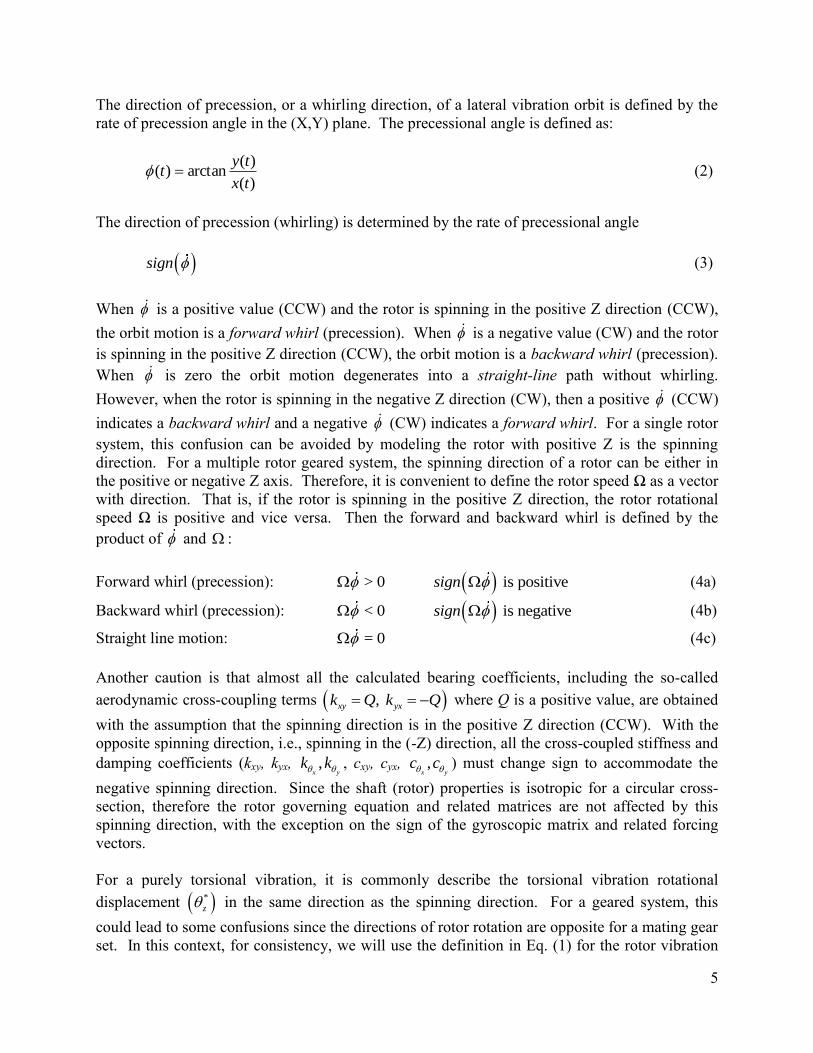
Since this system is an isotropic system with speed independent (constant) bearing coefficients,

the critical speeds can also be estimated using the critical speed analysis. The critical speeds due

to rotor 1 mass unbalance are obtained by assigning the spin(1)/whirl ratio = 1, i.e. 1 1

and

2 1.5

. And the critical speeds due to rotor 2 mass unbalance are obtained by assigning the

spin(2)/whirl ratio = 1, i.e. 1 10.66667

1.5

and 2 1

. The associated mode shapes are

shown in Figure 1-4.

Figure 1-4 Critical speed mode shapes for 2 11.5

The rotor steady state responses at station 2 (rotor 1) and station 9 (rotor 2) are shown in Figure

1-5. As expected, the peak responses due to rotor 1 mass unbalance occur around (Ω1=8250,

Ω2=12375 rpm) and (Ω1=15292, Ω2=22938 rpm) and the peak responses due to rotor 2 mass

unbalance occur around (Ω1=5233, Ω2=7849 rpm) and (Ω1=10062, Ω2=15093 rpm). To fully

understand the rotor motion with both mass unbalances, a transient analysis is performed at the

rotor speed of 1 10,000 and 2 15,000 rpm with both the mass unbalance forces from

12

rotors 1 and 2 included. The steady state results are presented in Figure 1-6. Both rotors are

whirling in the CCW direction, which is the same as the rotor direction of rotation, with two

whirl frequencies of 10,000 and 15,000 rpm, which are caused by the rotor mass unbalances.

The steady state motion is not a single harmonic vibration with simple elliptical orbit, it is the

sum of two harmonics and the whirling direction is the same as the rotor rotational direction, as

shown in Figure 1-6.

Figure 1-5 Rotor responses for 2 11.5

13

Figure 1-6 Rotor responses at speed Ω1=10000 and Ω2=15000 rpm

14

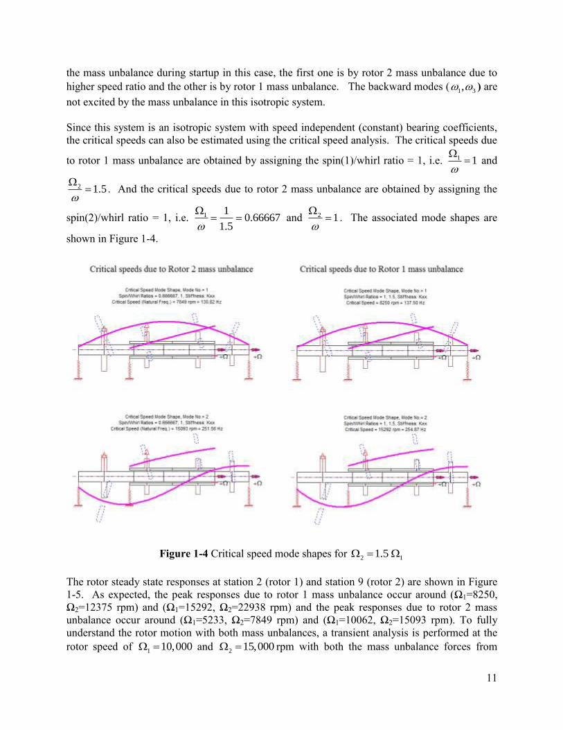
Case 2: 2 11.5 , Ω1: CCW and Ω2: CW

Let us consider the rotor 2 is counter-rotation of rotor 1, that is, rotor 1 rotates CCW and rotor 2

rotates CW, as shown in Figure 1-7. The resulted first 4 natural frequencies ( 2 11.5 ) are

overlapped with the original first 4 natural frequencies ( 2 11.5 ) shown in Figure 1-8.

The associated 4 mode shapes at speed of Ω1=10000, Ω2=-15000 rpm shown in Figure 1-9. Note

that the first and third modes, as shown in Figure 1-9, are whirling CW in the negative Z axis,

which are backward precessions for rotor 1, however, are forward precessions for rotor 2. And

the second and fourth modes are whirling CCW in the positive Z axis, which are forward

precessions for rotor 1 and backward precessions for rotor 2. Since the rotor 2 rotates CW which

has the opposite gyroscopic effect from rotor 1, therefore, the two modes ( 1 2, ) and ( 3 4, )

split less than that in Case1 with the same direction of rotation. The gyroscopic effect from rotor

1 stiffens the second and fourth modes since they are forward precessions for rotor 1. However

these two modes are softened by the gyroscopic effect from rotor 2 since they are backward

precessions for rotor 2. Same discussions apply for the other two modes. Again, for the

isotropic systems, the mass unbalance excites the forward modes, which whirl in the same

direction as the rotor direction of rotation. Therefore, the mass unbalance of rotor 1 excites the

modes ( 2 4, ) with CCW whirling direction and the mass unbalance of rotor 2 excites the

modes ( 1 3, ) with CW whirling direction. So, each mode will be excited once during rotor

startup in this case, which is different from Case 1.

15

Figure 1-7 Dual rotor system, 2 11.5 , Ω1: CCW and Ω2: CW

Figure 1-8 Whirl speed map for 2 11.5 and 2 11.5

The critical speeds due to rotor 1 mass unbalance are obtained by assigning the spin(1)/whirl

ratio = 1, i.e. 1 1

and 2 1.5

. And the critical speeds due to rotor 2 mass unbalance are

16

obtained by assigning the spin(2)/whirl ratio = 1, i.e. 2 1

and 1 1

0.666671.5

. The

associated mode shapes are shown in Figure 1-10.

Figure 1-9 Precessional mode shapes at speed of Ω1=10000, Ω2= -15000 rpm

Figure 1-10 Critical speed mode shapes for 2 11.5

17

The rotor responses at station 2 (rotor 1) and station 9 (rotor 2) due to mass unbalance are shown

in Figure 1-11. As expected, the peak responses occur at the critical speeds which are different

from Case 1. Figure 1-12 shows the rotor steady state response with both mass unbalances at

speed of (Ω1=10000 rpm CCW and Ω1=15000 rpm CW). It shows that the rotor 1 is whirling

CCW and rotor 2 is whirling CW, both are corresponding to their own direction of rotation.

Again, the whirling frequencies are the rotor speeds due to mass unbalances.

Figure 1-11 Rotor responses for 2 11.5

18

Figure 1-12 Rotor responses at speed Ω1=10000 rpm CCW and Ω2=15000 rpm CW

19

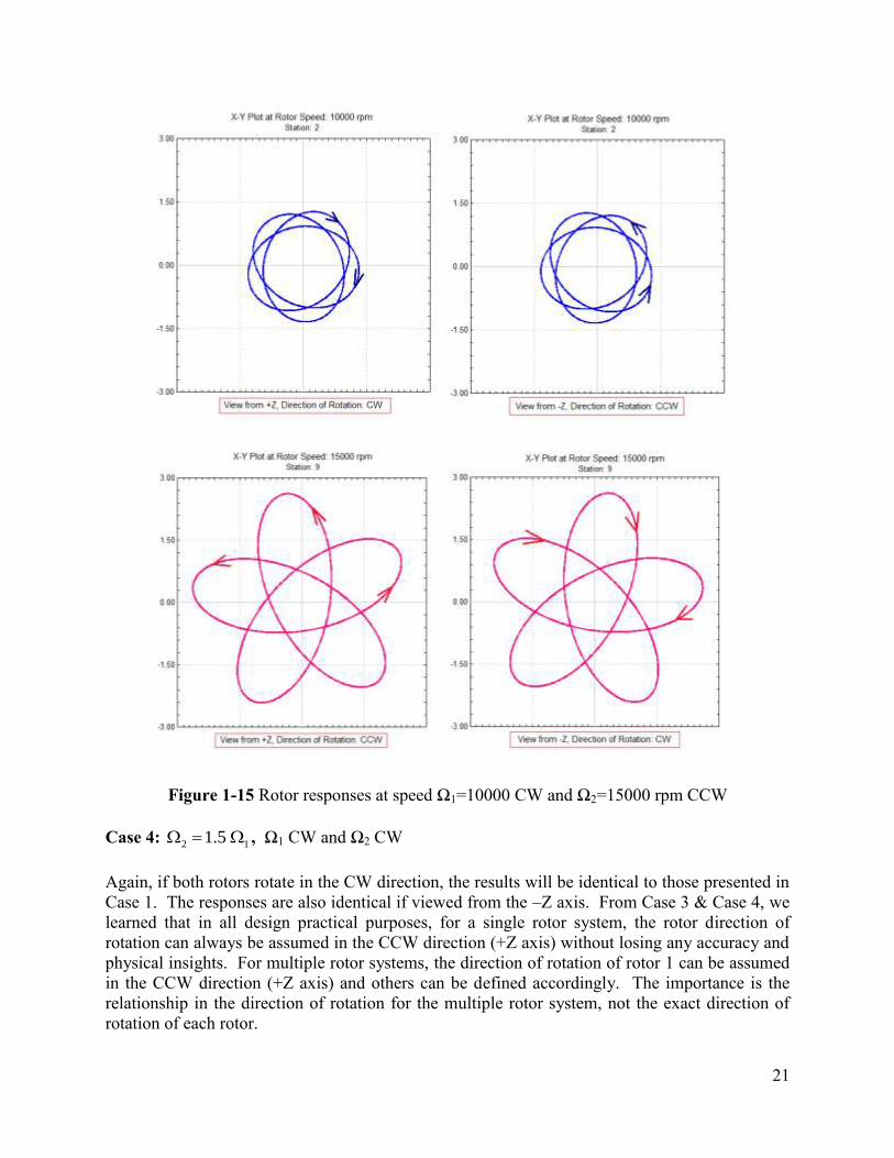
Case 3: 2 11.5 , Ω1 CW and Ω2 CCW

For the completeness of the comparison, let us assume that the rotor 1 rotates CW and rotor 2

rotates CCW, as shown in Figure 1-13. The whirl speed map is shown in Figure 1-14. Note that

the curves are generated from Case 3 and dots represent the results from Case 2. It shows that

the frequency values are identical, however, the whirling direction are opposite, but consistent

with the rotor direction of rotation. Therefore, the critical speeds due to rotor mass unbalances

are identical to those in case 2, since the mass unbalance excites the forward modes, which whirl

in the same direction as the rotor rotation. The critical speeds calculated using the critical speed

analysis are also identical to those obtained in Case 2 and are not repeated here. The steady state

unbalance responses are also the same as those in Case 2 Figure 1-11. Figure 1-15 shows the

steady state responses at station 2 (rotor 1) and station 9 (rotor 2) at rotor speed of (Ω1=10000

rpm CW and Ω1=15000 rpm CCW) viewing from the +Z and –Z axis. Again, the response orbits

whir in the same direction as the rotor rotation due to mass unbalance in this isotropic system.

20

Figure 1-13 Dual rotor system, 2 11.5 , Ω1: CW and Ω2: CCW

Figure 1-14 Whirl speed map for 2 11.5 , Ω1: CW and Ω2: CCW

21

Figure 1-15 Rotor responses at speed Ω1=10000 CW and Ω2=15000 rpm CCW

Case 4: 2 11.5 , Ω1 CW and Ω2 CW

Again, if both rotors rotate in the CW direction, the results will be identical to those presented in

Case 1. The responses are also identical if viewed from the –Z axis. From Case 3 & Case 4, we

learned that in all design practical purposes, for a single rotor system, the rotor direction of

rotation can always be assumed in the CCW direction (+Z axis) without losing any accuracy and

physical insights. For multiple rotor systems, the direction of rotation of rotor 1 can be assumed

in the CCW direction (+Z axis) and others can be defined accordingly. The importance is the

relationship in the direction of rotation for the multiple rotor system, not the exact direction of

rotation of each rotor.

22

Example 2: A single rotor with cross-coupled bearing coefficients

Before we move on to the geared rotor system with multiple rotors running in different speeds

and directions, let us examine another example to understand the coordinate relationship in more

details. Consider a uniform shaft supported by two identical fluid film bearings, as shown in

Figure 2-1. This system was first presented by Lund (1974) using the linearized bearing

coefficients in the determination of damped critical speeds and instability threshold. It was then

fully analyzed by Chen & Gunter (2005) in both linear and nonlinear analysis and results are

well documented. This example used here is to address some necessary requirements and

cautions in the coordinate transformation, in preparation for the analysis of complicated multiple

shaft systems.

This uniform shaft has a length of 50 in., a diameter of 4 in., a Young’s modulus of 3.0E07 psi, a

shear modulus of 1.154E+07 psi, and a weight density of 0.283 Lb/in3, is supported at the ends

by two identical plain cylindrical fluid film bearings. For this uniform shaft, it has been

demonstrated that the shaft shear deformation, rotatory inertia, and gyroscopic effects have a

minimal influence on the dynamics of this rotor system, therefore, they are neglected here and

focus is on the coordinate transformation. The two fluid film bearings are plain cylindrical

journal bearings with a journal diameter of 4 in., a bearing radial clearance of 0.002 in., a bearing

axial length of 1 in., and an oil viscosity of 6.9 centiPoise (1.0E-06 Reyns).

Figure 2-1 Uniform shaft supported by two plain cylindrical bearings

To perform the linear analysis on this rotor system, we need to analyze the bearings first to

obtain the linearized bearing coefficients. Two bearing coordinate systems, as shown in Figure

1-2, are commonly used in the bearing analysis. The first one (X,Y), commonly used by the

rotor dynamics analysts, is the same as the rotor coordinate system, that is X to the right and Y to

the top and Z points to the viewer, regardless the bearing load vector. Then the bearing

coefficients can be directly used in the rotor dynamic analysis. The second one (x’,y’) is more

frequently used by the bearing analysts where x’-axis is the same as the load vector and y’ is

perpendicular to the x’-axis. Once the linearized bearing coefficients are obtained from the

(x’,y’) coordinates system, it can be easily transformed into the standard (X,Y) coordinate system

for the rotordynamic study. This coordinate transformation is described in details in Chen and

Gunter and is given in Eq. 2-1.

23

Figure 2-2 Bearing coordinates

' ' ' '

' ' ' '

cos sin cos sin

sin cos sin cos

xx xy x x x y

yx yy y x y y

k k k k

k k k k

where is the angle from x’ to X axis. One critical assumption used in the above two coordinate

systems for the bearing analysis is that the shaft direction of rotation is CCW in the Z direction.

This assumption was not emphasized in many textbooks and papers, because for a single rotor

system, we can always model the rotor system in the CCW direction of rotation without any

problem as described in previous example. However, there will be different direction of

rotations present for a geared system. Then caution needs to be taken to be sure that all the

bearing coefficients have been converted into the coordinate system used for the rotor analysis.

Two scenarios are considered and shown in Figure 2-3, where (X,Y) are now the coordinates

used to describe the rotor motion in the rotor dynamics analysis, and (Xb,Yb) are the coordinates

where the bearing linearized coefficients are obtained. When the rotor rotates CCW and the

bearing coefficients are calculated based on the assumption of CCW shaft rotation, then (X,Y)

and (Xb,Yb) are the same, there is no need for any transformation and the bearing coefficients can

be applied directly in the rotordynamic study. When the rotor rotates CW and the bearing

coefficients are calculated based on the assumption of CCW shaft rotation, then the X and Xb are

opposite to each other and Y and Yb are the same. The linearized bearing forces acting on the

rotor in both coordinate systems are:

In bearing coordinate system:

x xx xy xx xy

y yx yy yx yyb bb b b

F k k c cx x

F k k c cy y

In rotor coordinate system:

24

x xx xy xx xy

y yx yy yx yy

F k k c cx x

F k k c cy y

Since we have the bearing forces and linearized coefficients in the bearing coordinate system and

they need to be converted into the rotor coordinate system. The displacement, force, and

coefficients transformations for scenario 2 are:

Figure 2-3 Rotor coordinates and bearing coordinates

1 0

0 1b b

x x x

y y y

1 0

0 1

x x x

y y yb b

F F F

F F F

and

xx xy xx xy

yx yy yx yy b

k k k k

k k k k

xx xy xx xy

yx yy yx yy b

c c c c

c c c c

For the stiffness and damping coefficients, only changes are the sign for the cross-coupled

coefficients. The sign switch in the cross-coupled stiffness coefficients plays an important role

in the rotor stability analysis. It is known that the cross-coupled stiffness coefficients generate

the undesirable circulatory force and it contributes positive work done on the rotor system for a

whirling orbit in the positive Z direction (CCW whirling orbit), and negative work done for a

whirling orbit in the negative Z direction (CW whirling orbit). Positive work done indicates the

25

destabilizing effect and negative work done indicates the stabilizing effect. The work done by

the cross-coupled stiffness coefficients over one cycle of a harmonic motion is given before and

repeated here for easy reference:

circulatory xy yxW k k a b

where a and b are the semi-major and semi-minor axes of the elliptical orbit. Positive b indicates

a CCW whirling orbit and negative b indicates a CW whirling orbit. a b is the area of the

whirling elliptical orbit and positive area for a CCW whirling orbit and negative area for a CW

whirling orbit. With the positive ( yxxy kk ) term, this circulatory force destabilizes the CCW

whirling modes, and stabilizes the CW whirling modes. Since for a single rotor system, we can

always assume the rotor rotates CCW, therefore the CCW whirling modes are the so-called

forward modes and CW whirling modes are backward modes. However, for a CW shaft rotation,

the CW whirling modes are now the forward precessional modes and CCW whirling modes are

the backward precessional modes. For the fixed-lobe fluid film bearings, with the positive Z

shaft rotation, the ( yxxy kk ) term is prone to be positive for the high speed and low load

applications and it will tend to destabilize the forward modes with CCW precession. However, if

the bearing coefficients are obtained based on the negative Z shaft rotation, then the ( yxxy kk )

term is prone to be negative for the high speed and low load applications and it will tend to

destabilize the forward modes with CW precession. Therefore, the sign switch in the cross-

coupled stiffness coefficients is extremely important in the rotor stability analysis if the bearing

is analyzed in the CW rotation. This is also valid for the so-called aerodynamic cross-coupling

term Q used in the stability analysis by many Industry Standards, such as API. The purpose of

introducing the aero-dynamic cross-coupling is to study the rotor stability and its sensitivity to

the destabilizing force. The aerodynamic cross-coupling term is commonly treated (modeled) as

a pseudo bearing with the following stiffness expression:

0

0

Q

Q

where Q is a positive value.

However, the Standard did not mention that it is customary to assume that the rotor is rotating

CCW in the positive Z direction when the above expression is applied. If the rotor rotates in the

CW direction, then the proper aerodynamic cross-coupling expression will be:

0

0

Q

Q

where Q is a positive value and is CW rotation.

The aerodynamic cross-coupling term always destabilizes the forward modes, regardless the

shaft rotation. The above discussion will be illustrated using this example. The bearing

coefficients versus speeds and their coordinate definition are shown in Figure 1-4.

26


Case 1: is CCW rotation

Let us consider the conventional case, that is, the shaft is rotating CCW in the Z direction. Then,

the bearing coefficients can be directly applied in the rotor dynamic study. Figures 2-5 and 2-6

show the whirl speed map and stability map. These two maps have been presented in this text

many times. The only addition in the map is the direction of whirling for each mode. Since the

rotor is rotating in the CCW direction, so the modes with CCW precessions are the forward

modes, and with CW precessions are the backward modes. The first two backward modes are

overdamped and not shown in the map. The first forward mode goes to unstable when the rotor

speed exceeds 9120 rpm, which is commonly referenced as the instability threshold.

27



28

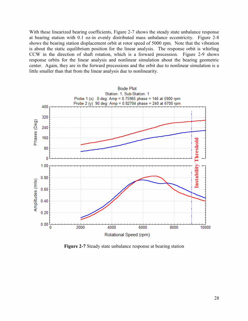
With these linearized bearing coefficients, Figure 2-7 shows the steady state unbalance response

at bearing station with 0.1 oz-in evenly distributed mass unbalance eccentricity. Figure 2-8

shows the bearing station displacement orbit at rotor speed of 5000 rpm. Note that the vibration

is about the static equilibrium position for the linear analysis. The response orbit is whirling

CCW in the direction of shaft rotation, which is a forward precession. Figure 2-9 shows

response orbits for the linear analysis and nonlinear simulation about the bearing geometric

center. Again, they are in the forward precessions and the orbit due to nonlinear simulation is a

little smaller than that from the linear analysis due to nonlinearity.

Figure 2-7 Steady state unbalance response at bearing station

29

Figure 2-8 Bearing station linear displacement orbit at 5000 rpm

Figure 2-9 Bearing station linear and nonlinear displacement orbit at 5000 rpm

30

Since the instability threshold is around 9120 rpm from the stability map, therefore, the linear

steady state unbalance response analysis is not valid after this speed and transient analysis is

required. Figure 2-10 shows the transient response orbit at 10000 rpm with the linearized

bearing coefficients. It shows that the response will grow out of the bearing clearance circle

which is not physically feasible in practice and it demonstrates that the linear theory is not valid

after the instability threshold and nonlinear theory should be applied. However, it shows that the

response grows in the CCW direction, same as the direction of shaft rotation. It implies that the

rotor is whirling with an unstable forward precessional mode, which is agreement with the

stability map. Figure 2-11 shows that response orbit with nonlinear simulation. Again, it shows

that the rotor is whirling CCW in the direction of shaft rotation, that is a forward precessional

motion. And the orbit is constrained within the bearing clearance circle.

Figure 2-10 Transient response with linearized bearing coefficients at 10000 rpm

31

Figure 2-11 Transient response with nonlinear bearing forces at 10000 rpm

The above discussion provides a brief review on some important concepts that were presented

before. The main objective here is to emphasize that the bearing coordinates and rotor

coordinates must be in the same direction of rotation. Let us consider now the rotor rotates in the

CW direction, as shown in Figure 2-12, and the bearing coefficients were obtained based on the

CCW direction of rotation as before. Figures 2-13 and 2-14 show the whirl speed map and

stability map with the original bearing coefficients. At the first glance, one may think that the

results are identical to the previous discussion due to the same frequency values and the mode

whirling directions, so it is unnecessary to switch the sign in the bearing cross-coupled

coefficients. However, it is also noted that the rotor now rotates in the CW direction, so the

CCW precessional modes becomes backward precessional modes and CW precessional modes

become forward precessional modes. So, with these incorrect bearing coefficients, the backward

mode becomes unstable, which is NOT the same as before. So, without the sing change in the

bearing coefficients, the free vibration analysis provides incorrect results.

32

Figure 2-12 Shaft rotation CW

Figure 2-13 Whirl speed map with the INCORRECT bearing data

33

Figure 2-14 Stability speed map with the INCORRECT bearing data

Figure 2-15 shows the steady state unbalance response at the bearing station with the original

bearing coefficients. Now, the significant difference is shown here with the previous result in

Figure 2-7. Figure 2-16 shows the bearing station steady state response orbit at 5000 rpm

viewed from both directions: +Z and –Z directions. It shows that the response orbit is whirling

in the opposite direction from the direction of shaft rotation. This is also incorrect compared

with previous results in Figure 2-8. Therefore, the sign switch in the bearing cross-coupled

coefficients is important and needs special attention when the shaft direction of rotation is

different from the bearing coefficients calculation.

34

Figure 2-15 Steady state response with the INCORRECT bearing data

Figure 2-16 Steady state response at 5000 rpm with the INCORRECT bearing data

Figures 2-17 and 2-18 show the whirl speed map and stability map with the correct bearing

coefficients, that is the sign change in the cross-coupled bearing coefficients. Now the results

are identical to the original results. Although the forward precessional modes now are whirling

in the CW direction, it is consistent with the shaft direction of rotation.

35

Figure 2-17 Whirl speed map with CORRECT bearing data

Figure 2-18 Stability map with CORRECT bearing data

36

The steady state unbalance response in Bode plot is identical to the correct result shown in

Figure 2-7, and not shown here. The response orbit at bearing station at 5000 rpm and viewed

from both +z and –Z directions, are shown in Figure 2-19. It shows that the results are identical

to previous results if viewed from the correct direction. This example illustrates the importance

of the shaft direction in the bearing coefficient calculation. In the rotordynamic study, the rotor

rotation must be consistent with the bearing coefficients.

Figure 2-19 Bearing station response orbit with CORRECT bearing data

37

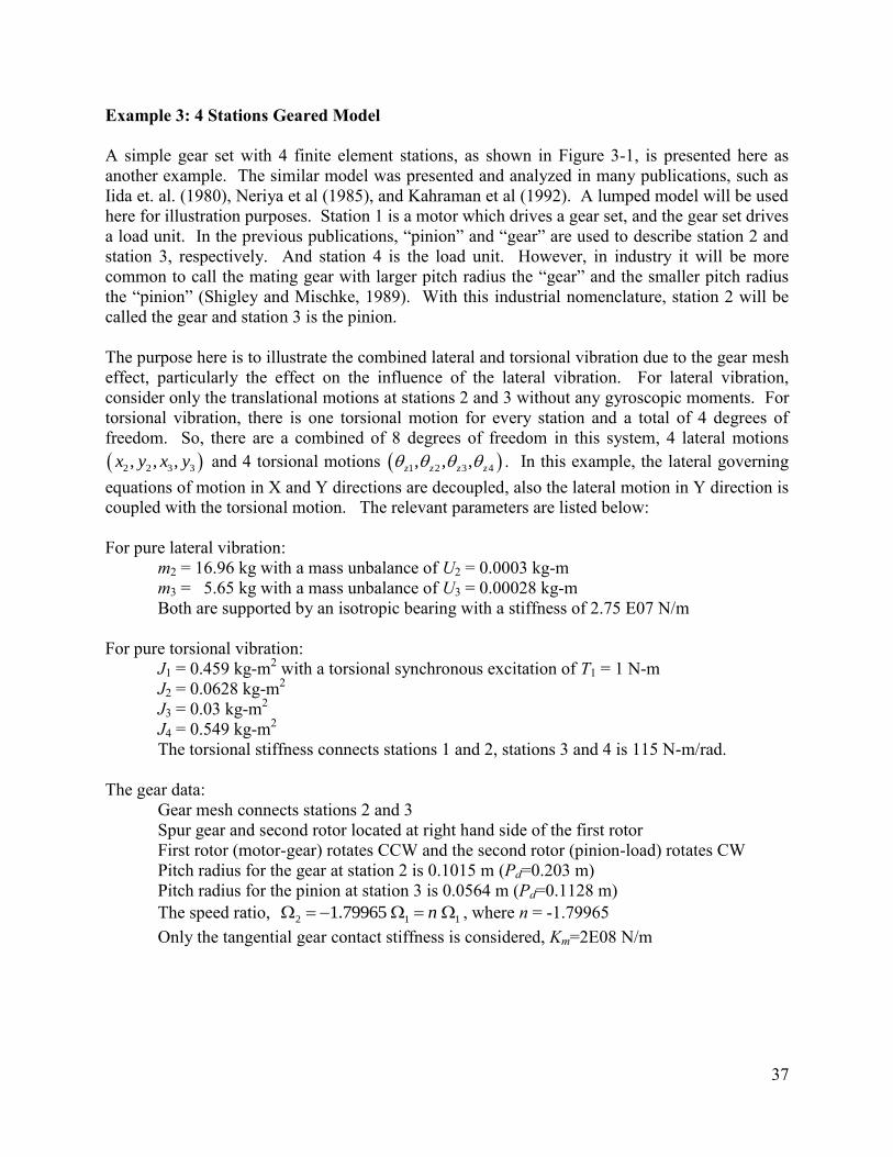
Example 3: 4 Stations Geared Model

A simple gear set with 4 finite element stations, as shown in Figure 3-1, is presented here as

another example. The similar model was presented and analyzed in many publications, such as

Iida et. al. (1980), Neriya et al (1985), and Kahraman et al (1992). A lumped model will be used

here for illustration purposes. Station 1 is a motor which drives a gear set, and the gear set drives

a load unit. In the previous publications, “pinion” and “gear” are used to describe station 2 and

station 3, respectively. And station 4 is the load unit. However, in industry it will be more

common to call the mating gear with larger pitch radius the “gear” and the smaller pitch radius

the “pinion” (Shigley and Mischke, 1989). With this industrial nomenclature, station 2 will be

called the gear and station 3 is the pinion.

The purpose here is to illustrate the combined lateral and torsional vibration due to the gear mesh

effect, particularly the effect on the influence of the lateral vibration. For lateral vibration,

consider only the translational motions at stations 2 and 3 without any gyroscopic moments. For

torsional vibration, there is one torsional motion for every station and a total of 4 degrees of

freedom. So, there are a combined of 8 degrees of freedom in this system, 4 lateral motions

2 2 3 3, , ,x y x y and 4 torsional motions 1 2 3 4, , ,z z z z . In this example, the lateral governing

equations of motion in X and Y directions are decoupled, also the lateral motion in Y direction is

coupled with the torsional motion. The relevant parameters are listed below:

For pure lateral vibration:

m2 = 16.96 kg with a mass unbalance of U2 = 0.0003 kg-m

m3 = 5.65 kg with a mass unbalance of U3 = 0.00028 kg-m

Both are supported by an isotropic bearing with a stiffness of 2.75 E07 N/m

For pure torsional vibration:

J1 = 0.459 kg-m2 with a torsional synchronous excitation of T1 = 1 N-m

J2 = 0.0628 kg-m2

J3 = 0.03 kg-m2

J4 = 0.549 kg-m2

The torsional stiffness connects stations 1 and 2, stations 3 and 4 is 115 N-m/rad.

The gear data:

Gear mesh connects stations 2 and 3

Spur gear and second rotor located at right hand side of the first rotor

First rotor (motor-gear) rotates CCW and the second rotor (pinion-load) rotates CW

Pitch radius for the gear at station 2 is 0.1015 m (Pd=0.203 m)

Pitch radius for the pinion at station 3 is 0.0564 m (Pd=0.1128 m)

The speed ratio, 2 1 11.79965 n , where n = -1.79965

Only the tangential gear contact stiffness is considered, Km=2E08 N/m

38

Figure 3-1 4-stations geared system

Gear mesh data is entered under the Torsional/Axial tab in the Data Editor option. In this

example, the tangential stiffness is given and it is a spur gear, therefore there is no need to enter

the pressure angle and helix angle. All other data can be entered just like doing the pure lateral

and torsional analysis. When performing the Lateral-Torsional-Axial analysis option, one may

select the types vibration be included in the analysis. In this example, Axial vibration is always

be excluded, and torsional and lateral are included.

39

40

Both the free and forced vibrations are studied. For free vibration (natural frequency analysis),

four cases are included.

1. The first case is the conventional purely torsional analysis with a rigid link in the gear

mesh ( )mK . With this rigid link between stations 2 and 3, the original 4 DOF

torsional model has been reduced and become a 3 DOF torsional model. There are 3

natural frequencies are calculated: 0, 148, and 546 rpm. The zero natural frequency

corresponds to the rigid body motion due to unconstrained torsional motion.

2. The second case is the torsional analysis with the flexible gear mesh (Km=2E08 N/m).

There are 4 natural frequencies: 0, 148, 546, and 70185 rpm. The 4th

natural frequency is

introduced by the flexibility of the gear mesh and this frequency value is extremely high.

The 2nd

and 3rd

frequencies are essentially the same as the originally rigidly linked case.

It is typically true that the torsional stiffness due to the gear mesh is much higher than the

shaft torsional stiffness, and a rigid link can be reasonably assumed for the torsional

analysis.

3. The third case is the purely lateral vibration. Since the bearings are isotropic and there are 2

natural frequencies for each rotor, one for each direction. The natural frequencies for rotors 1

and 2 can be easily determined by the following frequency equation: k

m

a. Rotor 1: 2.75 07

1273 rad/sec = 12160 rpm16.96

x y

E

b. Rotor 2: 2.75 07

2206 rad/sec = 21068 rpm5.65

x y

E

41

4. The fourth case is the combination of the lateral and torsional vibration with the gear

mesh effect. Once the gear mesh is included, the system is no longer an isotropic system.

Asymmetry property is introduced by the gear mesh stiffness.

The results are summarized below:

Purely

Torsional

( )mK

Purely

Torsional

(Km=2E08 N/m)

Purely

Lateral

Combined

Torsional &

Lateral

Comments

Mode 0 0 0 0 Torsional Rigid Body

Mode 1 148 148 148 Torsional + weak y

Mode 2 546 546 546 Torsional + weak y

Mode 3 12160 10703 Lateral y2 + Torsional

Mode 4 12160 12160 Lateral x2

Mode 5 21068 17327 Lateral y3 + Torsional

Mode 6 21068 21068 Lateral x3

Mode 7 70185 96985 Torsional + Lateral y

The eigenvectors (modal displacements) for the vibratory modes are arranged in the following

order, 2 2 3 3 1 2 3 4, , , , , , ,z z z zx y x y , with translation motion first and then the torsional motion.

However, for clarity and easy interpretation, the torsional displacements in rotor 2 are commonly

converted into the equivalent displacements with the speed ratio. That is the torsional

displacements 3 4,z z will be expressed as 3 4,z z

n n

, where n = -1.79965. The modal

displacements are summarized in the following table and shown in the Figure 3-2.

Displ. Mode 1

148 rpm

Mode 2

546 rpm

Mode 3

10703 rpm

Mode 4

12160 rpm

Mode 5

17327 rpm

Mode 6

21068 rpm

Mode 7

96985 rpm

x2 0 0 0 1 0 0 0

y2 -4.0E-05 1.6E-05 -0.108 0 0.0617 0 0.0319

x3 0 0 0 0 0 1 0

y3 4.0E-05 -1.6E-05 0.033 0 0.197 0 0.0988

z1 1 0.0462 -0.0002 0 -6.5E-05 0 -2.1E-06

z2 0.0397 -0.5560 0.8580 0 0.8590 0 0.8600

z3/n 0.0389 -0.5557 -0.5557 0 -0.5557 0 -0.5557

z4/n -0.2617 0.0381 0.0001 0 0.0000 0 1.1E-06

z3 -0.0700 1 1 0 1 0 1

z4 0.4710 -0.0685 -0.0002 0 -0.0001 0 -2.0E-06

42

43

44

Figure 3-2 Mode shapes

It shows that mode 1 and mode 2 are primary torsional motions, there is extremely small relative

torsional motion occurs at station 2 and 3 2 3, /z z n which causes insignificant movements at

y direction for stations 2 and 3. The frequencies are basically the same as the purely torsional

analysis without the lateral vibration. Again, in this example, only the lateral motion in Y

direction is coupled with the torsional motion and lateral motion in X direction is decoupled

from other motions.

The mode 3 shows the strong coupling between the torsional motion and the lateral motion of

rotor 1 and again only in the y direction. Mode 5 shows the strong coupling between the

torsional motion and the lateral motion of rotor 2 and also only in the y direction. Due to the

large relative movement at the gear contact point, it acts like a flexible support underneath the

bearings, so the frequencies are lower than those obtained from the pure lateral motion.

Modes 4 and 6 are the purely lateral motion at the X direction for the rotor 1 and rotor 2 and the

frequencies are the same as the pure lateral vibration. Mode 7 is the torsional motion coupled

with the weak lateral motion and it raises the frequency from the purely torsional motion.

Since there is no gyroscopic effect present and the bearings are isotropic, the system natural

frequencies do not vary with the rotor speed. Figure 3 shows the whirl speed map with both

rotor speeds are labeled in the X-axis. Each mode can be excited by the synchronous excitations.

The critical speeds for the first 6 modes below 25000 rpm of rotor 1 speed are summarized in

table 2.

45

Figure 3-3 Whirl speed map

Mode Critical speeds due to rotor 1

synchronous excitation

Critical speeds due to rotor 2

synchronous excitation

(rpm) Rotor 1 speed, Ω1 Rotor 2 speed, Ω2 Rotor 1 speed, Ω1 Rotor 2 speed, Ω2

148 148 Ω2 = 1.79965 Ω1 Ω1 = Ω2 / 1.79965 148

546 546 Ω2 = 1.79965 Ω1 Ω1 = Ω2 / 1.79965 546

10,703 10,703 Ω2 = 1.79965 Ω1 Ω1 = Ω2 / 1.79965 10,703

10 12,160 Ω2 = 1.79965 Ω1 Ω1 = Ω2 / 1.79965 12,160

17,327 17,327 Ω2 = 1.79965 Ω1 Ω1 = Ω2 / 1.79965 17,327

21,068 21,068 Ω2 = 1.79965 Ω1 Ω1 = Ω2 / 1.79965 21,068

46

Now, let us investigate the steady state synchronous response due to rotor 1 unbalance, rotor 2

unbalance, and motor torsional excitation. The objective here is to study the dynamic

characteristics of the system due to various excitations, and not focus on the exact response

amplitude since no damping is introduced in this system. The steady state response was

analyzed from 10 rpm to 25,000 rpm with an increment of 10 rpm.

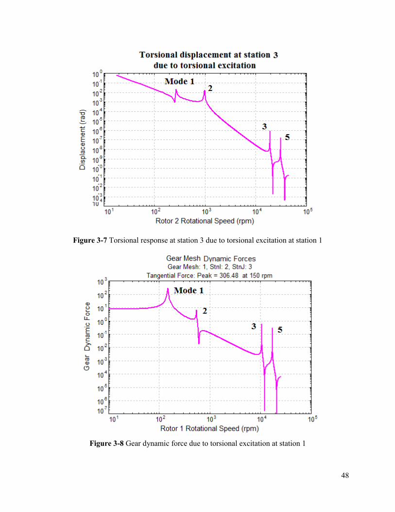
Case 1: Motor synchronous excitation, T1=1 N-m

With the torsional synchronous excitation at the motor (station 1), Figures 3-4 and 3-5 show the

lateral response at stations 2 (rotor 1) and 3 (rotor 2). As expected, the peaks were observed for

modes 1, 2, 3, and 5 with Y displacements only. There is no response for the X displacement

since the lateral-torsional coupling occurs in the Y displacement only in this rotor arrangement.

The responses are straight line motions. Modes 4 and 6 are the pure lateral vibration modes in

the X direction which are not excited by the torsional excitation. Figures 3-6 and 3-7 show the

torsional displacements at stations 2 and 3 and again only the modes 1, 2, 3, and 5 are excited.

Figure 3-8 shows the gear dynamic force due to this torsional excitation.

It is noted that although the bearings are isotropic, however the lateral orbits at stations 2 and 3

are straight line motion due to torsional effect and not circular as observed in lateral vibration

analysis only, which implies that with this torsional vibration coupling, the system is no longer

isotropic.

Figure 3-4 Lateral steady state response at station 2 due to torsional excitation at station 1

47


Figure 3-6 Torsional response at station 2 due to torsional excitation at station 1

48

Figure 3-7 Torsional response at station 3 due to torsional excitation at station 1

Figure 3-8 Gear dynamic force due to torsional excitation at station 1

49

Case 2: Rotor 1 mass unbalance excitation, U2 = 0.0003 kg-m

Figure 3-9 shows the lateral steady state response at station 2 due to rotor 1 unbalance. It shows

that there is only one peak in the X direction at mode 4 critical speed and two peaks in the Y

direction occurring at modes 3 and 5 critical speeds. These results are consistent with the

observation from the modal displacements (mode shapes). Again, the system is no longer

isotropic due to the coupled lateral and torsional motions and the orbits are highly elliptical near

critical speeds for station 2. Figure 3-10 shows the lateral steady state response at station 3 due

to rotor 1 unbalance. It shows that there are 2 peaks in the Y direction due to resonances at

modes 3 and 5. However there is no motion in the X direction. As explained before, the motion

in the X direction is not coupled with the torsional motion. The motion at station 3 due to rotor 1

unbalance is a straight line motions along the Y axis.

Figure 3-11 is the torsional response at station 2 due to rotor 1 unbalance. Figure 3-12 is the gear

dynamic force due to rotor 1 unbalance. Both figures show that the lateral and torsional motions

are strongly coupled for modes 3 and 5.

Further examine the station 2 lateral response orbits at various rotor speeds, as shown in Figure

3-13. At low speed, the orbit is near circular and forward precession which indicates that the

torsional influence is insignificant. As speed increases, the orbit becomes more elliptical and the

major axis is aligned with the Y axis. At mode 3 resonance, the motion becomes a straight line.

After resonance, the orbit becomes backward precession and the major axis gradually turns to be

in-line with the X-axis. After the mode 4 resonance, the orbit becomes forward precession again.

Figure 3-9 Lateral steady state response at station 2 due to rotor 1 unbalance

50


Figure 3-11 Torsional response at station 2 due to rotor 1 unbalance

51

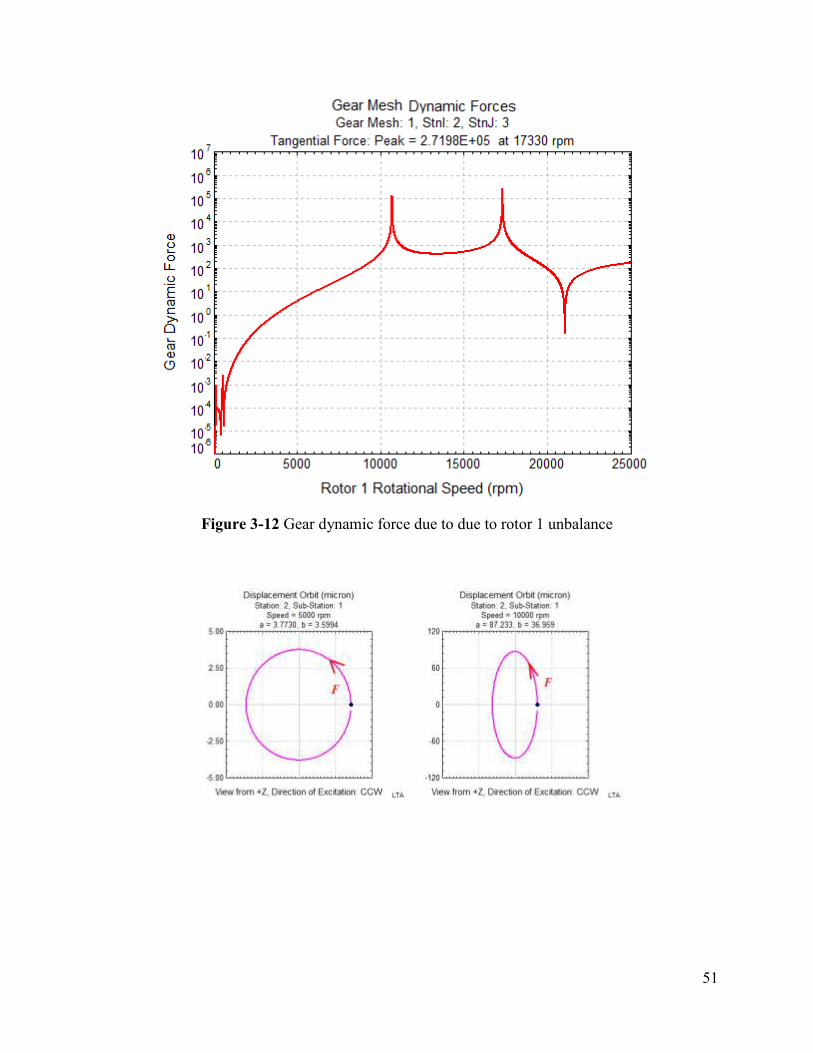
Figure 3-12 Gear dynamic force due to due to rotor 1 unbalance

52

Figure 3-13 Lateral response orbits at station 2 for various rotor speeds due to rotor 1 unbalance

Case 3: Rotor 2 mass unbalance excitation, U3 = 0.00028 kg-m

Now let us consider the steady state response due to rotor 2 mass unbalance at station 3 only.

Figure 3-14 shows the lateral steady state response at station 2 (rotor 1) due to rotor 2 unbalance.

It shows that the response at Y direction has two peaks due to modes 3 and 5 resonances, and the

response at X direction is null. So, the response at station 2 is a straight line motion along the Y

axis due to rotor 2 unbalance.

53

Figure 3-15 shows the lateral steady state response at station 3 (rotor 2) due to rotor 2 unbalance.

It shows that the response at Y direction has two peaks due to modes 3 and 5 resonances, and the

response at X direction has one peak due to mode 6 resonance. The discussions on this case are

similar to the previous case. Again, there are backward whirl between mode 5 and 6 at station 3.



54

Case 4: Angular position of rotor 2 is not zero

Note that the above discussion is based on the rotor 2 is at zero angular position in the horizontal

line from rotor 1, therefore the torsional motion couples the Y displacements only. Let us

consider another scenario that is the rotor 2 is located at 45 degree with respect to rotor 1, as

shown in Figure 3-16. Then, the torsional motion couples both X and Y directions. The values

of the system natural frequencies are identical to the previous case, except the X and Y lateral

motions are now both coupled with the torsional motion in modes 1, 2, 3, 5, and 7. Modes 4 and

6 are still purely lateral motions along the gear center line without torsional effect. Mode shapes

for modes 4, 5 and 6 are shown in Figure 3-17.

Figure 3-16 Rotor center line is not in the X-axis

55

Figure 3-17 Mode shapes for modes 4, 5, and 6

Next let us consider the forced response. Figure 3-18 is the steady state response at station 2 due

to the torsional excitation, same as case 1 discussed before. It shows that modes 1, 2, 3, 5 are

excited by the torsional excitation and purely lateral modes 4 and 6 are decoupled from the

torsional motion and not excited by the torsional excitation. The displacements in X and Y

directions have the same amplitude but different phase. The lateral response orbit now is a

straight line in 45 degree along the pressure line, as shown in Figure 3-19, not in Y direction as

discussed in case 1.

56


Figure 3-19 Lateral response orbit at station 2 due to torsional excitation at station 1

57

Figure 3-20 shows the lateral steady state response at station 2 due to rotor 1 unbalance. Again,

modes 3, 4, and 5 were excited by rotor 1 unbalance and the amplitudes in X and Y directions

are the same, but phases are different.


Figure 3-21 shows the lateral steady state response at station 3 due to rotor 1 unbalance. Modes

3 and 5 were excited by rotor 1 unbalance and the amplitudes in X and Y directions are the same,

but phases are different. Mode 4 is a purely lateral motion at station 2, therefore, not shown at

station 3 in Figure 3-21.

Again, although the bearings are isotropic, however, the orbits in general are not circular and

backward whirl exists between critical speeds. Figure 3-22 shows the response orbits at station 2

due to rotor 1 unbalance in various speeds. Again, backward whirl occurs between 2 critical

speeds.

It shows that the anisotropy of the support property is due to the effect of gear mating.

58


59

Figure 3-22 Lateral response orbits at station 2 for various speeds due to rotor 1 unbalance

60

Example 4: NASA test rig

A NASA test rig, shown in Figure 4-1, is used as a fourth example before we move on to an

industrial application. This spur geared system has been presented in numerous publications

(Kahraman, etal, 1990, 1992, Singh, et al, 1990). The natural frequencies at zero speed were

presented in all the publications and compared here. For comparison purpose, the shaft shear

deformation is neglected in the analysis. The 2 shafts have the same pitch radii (same speed).

The relevant parameters are shown in the Figure 4-1. To draw the a bearing using a block, go to

Project – Preferences Settings – Model Display Settings – Set Bearing Length = -1 or 0, then,

adjust the Bearing Width.

Figure 4-1 Two shafts system

To compare the results is an easy task and is not the only purpose here. The objective is to fully

understand the dynamics of a multiple rotor system using the available knowledge. It is strongly

recommended that each rotor should be analyzed before analyzing the entire system. At zero

speed, the first 4 natural frequencies of rotor 1 (driving shaft) are: 687, 687, 3387, and 3387 Hz.

The first 4 natural frequencies of rotor 2 (driven shaft) are: 695, 695, 3454, and 3454 Hz. These

8 natural frequencies can be obtained from analyzing each individual rotor or analyzing the

entire rotor model with lateral vibration analysis without gear mesh effect.

61

The mode shapes from analyzing the entire system without gear mesh are shown in Figure 4-2.

As expected that the first pair natural frequencies are corresponding to the first bending mode in

the X and Y directions, respectively. And the second pair natural frequencies are corresponding

to the second bending mode in the X and Y directions, respectively. Noted that the gears (disks)

are at the center of the shaft, therefore, the first two modes (the first bending mode) of each rotor

are not affected by the disk gyroscopic effect due to zero slope at disk. The third and fourth

modes (the second bending mode) of each rotor are strongly affected by the disk gyroscopic

effect due to large slope at disk. Further, the gears (disks) are at the nodal point for the second

bending modes, they are not influenced by the torsional vibration. This will be illustrated by the

whir speed map later.

62

Figure 4-2 Mode shapes for lateral vibration

The first purely torsional natural frequency of the entire system is 2136 Hz. Note that in this

mode each rotor acts as a rigid rotor and the only torsional flexibility is in the gear mesh. For

gear dynamics, this mode needs a great attention since the gears move out of phase. Also, this

mode will be influenced by the lateral-torsional coupling effect. The mode shape for this

torsional mode is shown in Figure 4.3.

63

Figure 4-3 Mode shape for torsional vibration

Table 1 summarizes the first several natural frequencies of the entire system (2 rotors) at zero

speed for comparison.

Mode Purely

Torsional

Rotor 1

Lateral

Rotor 2

Lateral

Combined

Lateral-

Torsional

NASA

GRD Mode Description

1 687 582 582 Lateral + Torsional

2 687 687 687 Lateral – Rotor 1 x

3 695 691 691 Lateral + Torsional

4 695 695 695 Lateral – Rotor 2 x

5 2136 2525 2531 Torsional + Lateral

6 3387 3387 3387 Lateral – Rotor 1

7 3387 3387 3387 Lateral – Rotor 1

8 3454 3454 3456 Lateral – Rotor 2

9 3454 3454 3456 Lateral – Rotor 2

The mode shapes for the first 5 modes with the combined lateral and torsional motions at zero

speed are shown in Figure 4-4. It shows that the first mode (582 Hz) is the combined lateral

motions of two rotors in Y direction with the torsional motion. Note that in this mode, rotor 1

and rotor 2 vibrates out of phase in the Y direction with large relative torsional displacements at

the gear contact. The second mode (687 Hz) is an uncoupled lateral motion (X direction) for

64

rotor 1. The third mode (691 Hz) is again a combined lateral and torsional mode. However,

unlike mode 1, both rotors now vibrate in phase in the Y direction with small relative torsional

displacements at gear contact in this mode. The fourth mode (695 Hz) is an uncoupled lateral

motion (X direction) for rotor 2. The fifth mode (2525 Hz) is a combined torsional and lateral

mode with very large relative torsional displacements at gear contact and small lateral motion in

Y direction for both rotors. Among these 5 modes, for the gear dynamic study, modes 1, 3, and 5

are of the critical modes, which coupled torsional and lateral motions. Modes 6, 7, 8, and 9 are

purely lateral vibration with nodal point at the gear location, therefore, no influence from the

torsional motion on these modes.

65

Figure 4-4 Mode shape for the combined system

66

The whirl speed map for the first 9 natural frequencies is shown in Figure 4-5. It shows that the

gyroscopic effect has little influences on the lowest 5 modes, since the disks (gears) are at the

center of shafts with zero gyroscopic moments in these modes. However, the gyroscopic effect

is significant as speed increases in modes 6, 7, 8, and 9 due to large slope at the gears.

Figure 4-5 Whirl speed map for 2 shafts system

67

Example 5: A geared industrial compressor

An industrial 3 stages compressor driven by an electrical motor, as shown in Figures 5-1 and 5-2,

is used in this example. Again, it is strongly recommended that each rotor to be analyzed before

performing the lateral-torsional-axial coupled vibration. So, the combined effect can be studied

and also it will minimize unnecessary mistakes which may be caused in the complete system.

68

Figure 5-1 A geared compressor model

The bull gear rotates CCW when viewing from the air discharge side into the motor. Typically,

the bull gear rotor is designed such that the operating speed is far below the first critical speed

and can be reasonably considered as a rigid rotor. Since stability is not an issue for the bull gear

rotor, 2-axial grooved bearings or elliptical bearings are commonly used in bull gear rotor

bearings. For the compressor pinions, typically their operating speeds are above the critical

speeds. The first pinion has 2 stages compressor with a design speed of 30191 rpm. The stage 3

compressor is in the second pinion with a design speed of 42903 rpm. Both pinions are

supported by two 4-pads tilting pad bearings. Note that the rider ring (thrust collar) is used to

transfer the pinion thrust loads into the low speed bull gear thrust bearing. Due to the aero

thrusts, the thrust loads from the pinions are transmitted to bull gear from the collars at the motor

side. The entire rotor assembly is axially constrained by the bull gear thrust bearing, however

not constrained in torsional motion. Therefore there is one rigid body torsional mode with zero

frequency present.

To obtain the linearized bearing coefficients, we need to calculate the bearing loads first. The

bearing loads due to gear forces and aero thrusts, viewed from both sides, are shown in Figure 5-

2. It should be noted that almost every bearing analysis program is based on the CCW shaft

rotation for the bearing coefficients. Proper bearing orientation is extremely important to ensure

the bearing performance reflect the design intention. For the current tilting pad bearings, the

bearings are oriented such that the loads are between pads. The relevant bearing parameters are

given in Figure 5-3.

69

Figure 5-2 Bearing loads

70

Figure 5-3 Bearing data

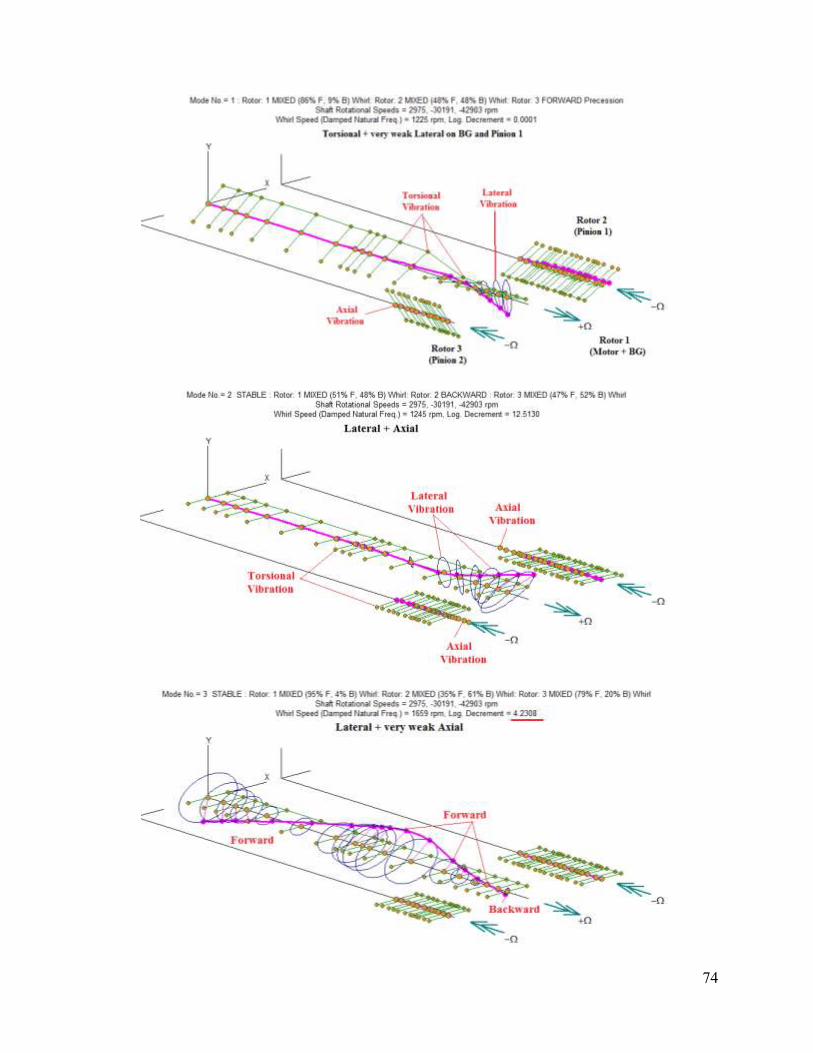
Again, in order to fully understand the dynamics of the entire rotor system, it is strongly

recommended that each rotor be analyzed separately first for the lateral vibration, as shown in

Figure 5-4. For the torsional analysis, the entire train must be considered and it has little

significance for the individual rotor to be analyzed for the torsional vibration since the torsional

motion for the first torsional mode is typically occurred around the coupling connected the driver

and driven unit.

71

Figure 5-4 Individual rotor model

72

Although the program is capable of including or neglecting the lateral, torsional, or axial

vibrations as shown below for the combined entire rotor system, it can also be used to verify the

results from the individual rotor analysis.

The natural frequencies at the motor design speed of 2975 rpm for the torsional, axial, individual

lateral, and combined effect are summarized in Table.

Mode Torsion Axial Motor + BG Pinion 1 Pinion 2 Combined Description

0 0 Torsional Mode

1 1225 1225 Torsional + very weak lateral on BG

2 1262 1245 Lateral BG + Axial

3 1657 1659 Lateral Motor + BG + weak Axial

4 1803 1803 Lateral Motor + weal Axial

5 3260 3220 Lateral BG + weak Axial

6 4892 4890 Lateral Motor + weak Axial

7 5287 5287 Lateral Motor + weak Axial

8 7262 7058 Lateral BG + Pinion 1 (high damping)

9 7631 7252 Lateral Pinion 1 (high damping)

10 7794 Overdamped in combined system

10 8576 8576 Axial motion only

11 11245 11292 Lateral Pinion 1



14 21064 20358 Lateral Pinion 1 & Pinion 2


16 21648 21543 21631 Lateral Driver + Axial

17 23304 23276 Lateral Driver + Pinion 1 + Axial

18

23909 Lateral Pinion 1

19 25080 26837 Lateral Driver

73

20 26943 26856 Lateral Driver + weak Axial

21 27042 30809 Lateral Pinion 1 + Driver


23 33185 39979 Lateral + Torsional + Axial



26 42102 42285 Torsional + Lateral + Axial

27 42282 47446 Lateral Pinion 1 + Pinion 2

28 43393 50045 Lateral Pinion 1 + Pinion 2


The mode shapes for some interesting modes of the combined effects are shown in Figure 5-5

and brief discussion is also provided.

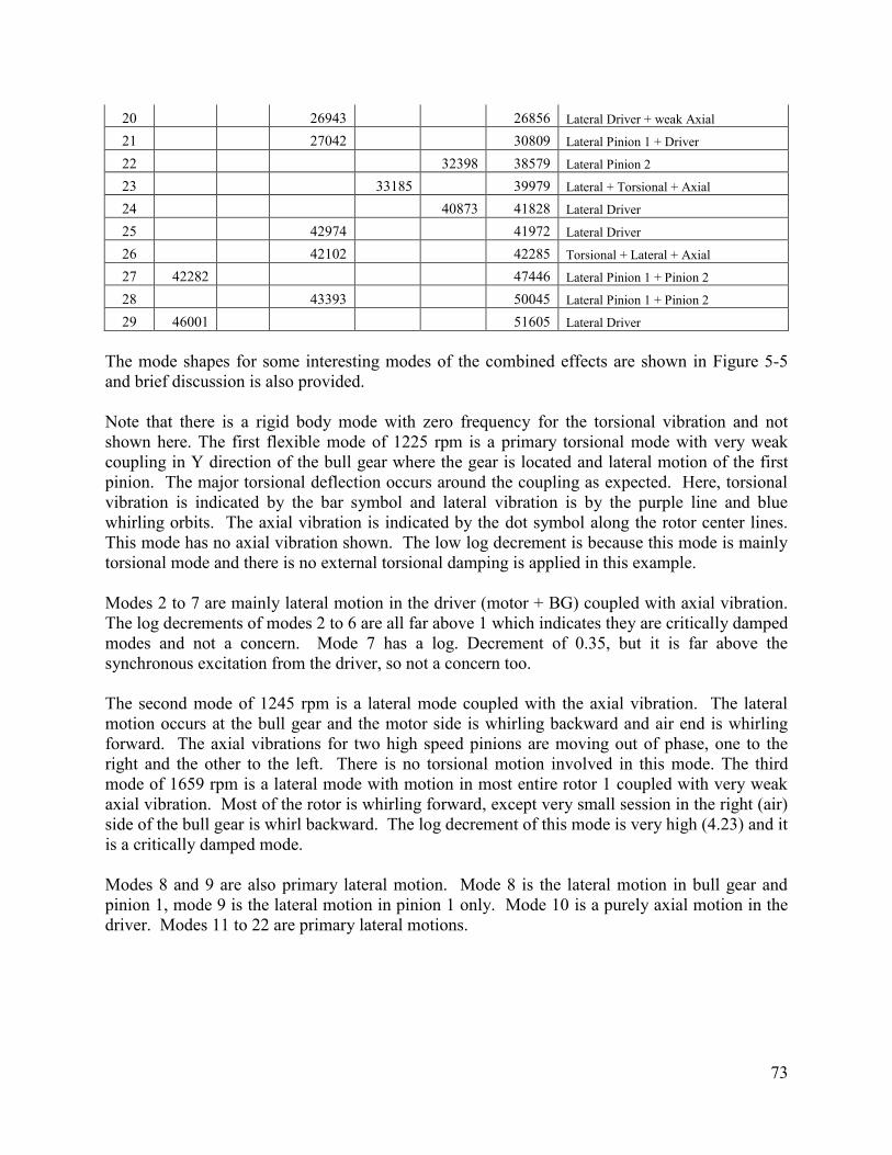
Note that there is a rigid body mode with zero frequency for the torsional vibration and not

shown here. The first flexible mode of 1225 rpm is a primary torsional mode with very weak

coupling in Y direction of the bull gear where the gear is located and lateral motion of the first

pinion. The major torsional deflection occurs around the coupling as expected. Here, torsional

vibration is indicated by the bar symbol and lateral vibration is by the purple line and blue

whirling orbits. The axial vibration is indicated by the dot symbol along the rotor center lines.

This mode has no axial vibration shown. The low log decrement is because this mode is mainly

torsional mode and there is no external torsional damping is applied in this example.

Modes 2 to 7 are mainly lateral motion in the driver (motor + BG) coupled with axial vibration.

The log decrements of modes 2 to 6 are all far above 1 which indicates they are critically damped

modes and not a concern. Mode 7 has a log. Decrement of 0.35, but it is far above the

synchronous excitation from the driver, so not a concern too.

The second mode of 1245 rpm is a lateral mode coupled with the axial vibration. The lateral

motion occurs at the bull gear and the motor side is whirling backward and air end is whirling

forward. The axial vibrations for two high speed pinions are moving out of phase, one to the

right and the other to the left. There is no torsional motion involved in this mode. The third

mode of 1659 rpm is a lateral mode with motion in most entire rotor 1 coupled with very weak

axial vibration. Most of the rotor is whirling forward, except very small session in the right (air)

side of the bull gear is whirl backward. The log decrement of this mode is very high (4.23) and it

is a critically damped mode.

Modes 8 and 9 are also primary lateral motion. Mode 8 is the lateral motion in bull gear and

pinion 1, mode 9 is the lateral motion in pinion 1 only. Mode 10 is a purely axial motion in the

driver. Modes 11 to 22 are primary lateral motions.

74

75

76

Figure 5-5 Selected mode shapes

Now, let us examine the steady state synchronous response and compare the results between the

combined system and individual rotor. Figure 5-6 shows the steady state responses at stages 1 &

2 bearings from the individual rotor 2 (pinion 1) analysis. Note that since only single rotor is

analyzed and the bearings are 4-pads tilting bearing bearings, the response orbit are circular and

|X|=|Y|. If we analyze the entire 3-rotors system with only rotor 2 unbalance and neglect the gear

mesh and rider ring effects, then the results will be identical and not repeated here.

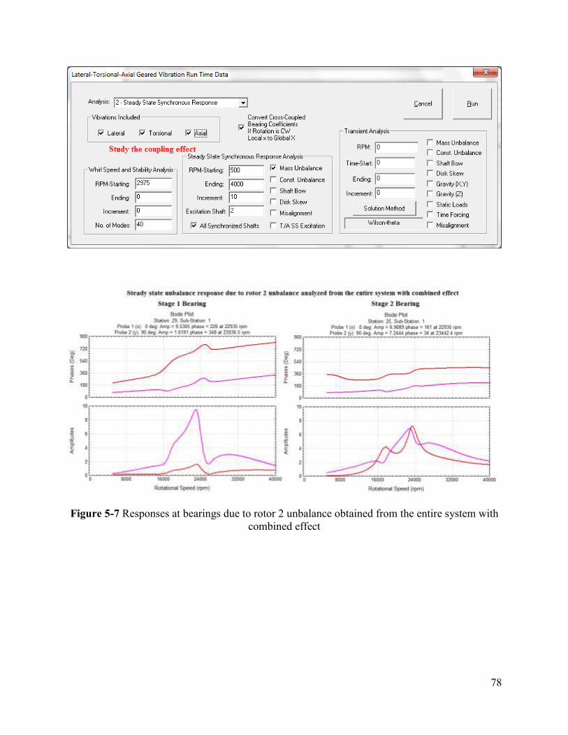
However, the interest is to study the coupled effect through the gear mesh and rider ring. Figure

5-7 shows the steady state responses due to rotor 2 unbalance at the same stations from the entire

train analysis with combined lateral-torsional-axial vibrations. With this lateral-torsional-and

axial coupling, the system is no longer isotropic and the x and y amplitudes are quite different.

As expected, when the rotor 2 goes through critical speed, it also excites rotor 1 and rotor 3

through the gear mesh and rider ring. Figure 5-8 shows the response at bull gear bearing and

stage 3 bearing due to rotor 2 unbalance. Although the vibration is small, it does exist. Figures

77

5-9 and 5-10 show the gear dynamic force between bull gear and rotor 2 and the collar axial

dynamic force due to vibration. It shows that the rider ring dynamic force is more than 10 times

higher than the gear mesh dynamic force. It is evident in some integrally geared compressors

with rider ring design, the vibration is strongly influenced by the rider ring effect.

Figure 5-6 Responses at bearings obtained from the individual rotor analysis

78

Figure 5-7 Responses at bearings due to rotor 2 unbalance obtained from the entire system with

combined effect

79

Figure 5-7 Responses at bull gear bearing and stage 3 bearing due to rotor 2 unbalance obtained

from the entire system with combined effect

Figure 5-10 Gear mesh dynamic force between rotor 1 and rotor 2

80

Figure 5-11 Thrust collar dynamic force between rotor 1 and rotor 2

Documents

Lateral-Torsional-Axial coupled vibration for a geared system