Embed Size (px)
Citation preview
Str
uct
ure
s R
ese
arc
h
Rep
ort
20
07
/5
22
90
Un
ivers
ity o
f Flo
rid
a
C
ivil
an
d C
oast
al
En
gin
eeri
ng
University of Florida
Civil and Coastal Engineering
Final Report July 2007
Lateral Bracing of Long-Span Florida Bulb-Tee Girders Principal investigators:
Gary R. Consolazio, Ph.D. H. R. (Trey) Hamilton, III, Ph.D., P.E. Research assistants:
Long Bui Jae Chung, Ph.D. Department of Civil and Coastal Engineering University of Florida P.O. Box 116580 Gainesville, Florida 32611 Sponsor: Florida Department of Transportation (FDOT) Marc Ansley, P.E. – Project manager Contract: UF Project No. 00052290 FDOT Contract No. BD-545 RPWO 36
i
Technical Report Documentation Page 1. Report No.
2. Government Accession No. 3. Recipient's Catalog No.
BD-545 RPWO-36 4. Title and Subtitle
5. Report Date July 2007 6. Performing Organization Code
Lateral Bracing of Long-Span Florida Bulb-Tee Girders
8. Performing Organization Report No. 7. Author(s) G. R. Consolazio, H. R. (Trey) Hamilton, III
2007/52290
9. Performing Organization Name and Address
10. Work Unit No. (TRAIS)
11. Contract or Grant No. BD-545 RPWO-36
University of Florida Department of Civil & Coastal Engineering P.O. Box 116580 Gainesville, FL 32611-6580
13. Type of Report and Period Covered
12. Sponsoring Agency Name and Address Final Report
14. Sponsoring Agency Code
Florida Department of Transportation Research Management Center 605 Suwannee Street, MS 30 Tallahassee, FL 32301-8064 15. Supplementary Notes
16. Abstract
The primary objectives of this research were to evaluate the lateral stability of long-span Florida bulb-tee girders during the bridge construction process and to offer recommendations for improving such stability. Numerical analysis techniques were used to quantify girder buckling capacities as functions of girder cross-sectional properties, span length, and bridge skew angle. In addition, the influences of factors such as girder sweep, bearing pad creep, and bracing stiffness were investigated as part of a comprehensive parametric study involving 4800 separate buckling analyses. Moderate-term (72 hour) bearing pad creep data were obtained from experimental testing and integrated into numerical analysis models. Results from the parametric study, and associated parameter sensitivity studies, indicated that girder buckling capacities are not strongly influenced by bearing pad creep, but are strongly influenced by the interaction of skew angle and girder slope. Simplified (and conservative) equations were then developed for use in assessing girder buckling strength under the combined effects of skew angle, field imperfections (e.g. sweep), and boundary conditions. A preliminary parametric study of limited scope was also carried out to assess girder stability under lateral wind pressure loading, again taking into account the effects of section type, span length, skew angle, and field conditions such as sweep. Based on results from the wind load parametric study, which involved 480 separate analyses, a preliminary wind capacity estimation equation was developed. 17. Key Words 18. Distribution Statement
Girder stability, buckling, imperfections, sweep, skew, camber, bearing pad, bracing stiffness, lateral torsional buckling, wind loading
No restrictions.
19. Security Classif. (of this report)
20. Security Classification. (of this page) 21. No. of Pages
22. Price
Unclassified Unclassified 96
Form DOT F 1700.7 (8-72). Reproduction of completed page authorized

ii
DISCLAIMER
The opinions, findings, and conclusions expressed in this report are those of the authors and not necessarily those of the State of Florida Department of Transportation.
ACKNOWLEDGEMENTS
The authors would like to thank the Florida Department of Transportation (FDOT) for providing the funding that made this research project possible. The authors would also like to thank the FDOT Structures Research Laboratory (Marc Ansley and Steve Eudy) for conducting bearing pad creep tests that yielded material parameter data for use in numerical models.

iii
TABLE OF CONTENTS
CHAPTER 1 INTRODUCTION .....................................................................................................1
1.1 Introduction................................................................................................................................1 1.2 Objectives ..................................................................................................................................3 1.3 Scope of work ............................................................................................................................3
CHAPTER 2 BACKGROUND .......................................................................................................5
2.1 Literature review........................................................................................................................5
CHAPTER 3 DESCRIPTION OF PHYSICAL SYSTEM............................................................10
3.1 Introduction..............................................................................................................................10 3.2 Terminology relating to geometric parameters........................................................................10 3.3 Bearing pads.............................................................................................................................12 3.4 Lateral bracing .........................................................................................................................14 3.5 Florida bulb-tee girder properties ............................................................................................15
CHAPTER 4 EXPERIMENTAL TESTING OF BEARING PADS.............................................17
4.1 Introduction..............................................................................................................................17 4.2 Description of experimental setup and loading procedures.....................................................17 4.3 Test results ...............................................................................................................................19 4.4 Elastic response of bearing pads to applied load .....................................................................21 4.5 Time-dependent creep response of bearing pads to sustained load .........................................21
CHAPTER 5 DETAILED 3D BEARING PAD MODELING......................................................25
5.1 Bearing pad model ...................................................................................................................25 5.2 Determination of material properties .......................................................................................26 5.3 Bearing pad stiffness determination.........................................................................................27
CHAPTER 6 SIMPLIFIED BEARING MODEL .........................................................................34
6.1 Introduction..............................................................................................................................34 6.2 Simplified bearing pad model..................................................................................................34
CHAPTER 7 BUCKLING ANALYSIS PROCEDURES.............................................................39
7.1 Introduction..............................................................................................................................39 7.2 Girder-buckling system model.................................................................................................39 7.3 Loading procedure used for buckling analysis ........................................................................41 7.4 Validation of large displacement buckling analysis procedure ...............................................43
iv
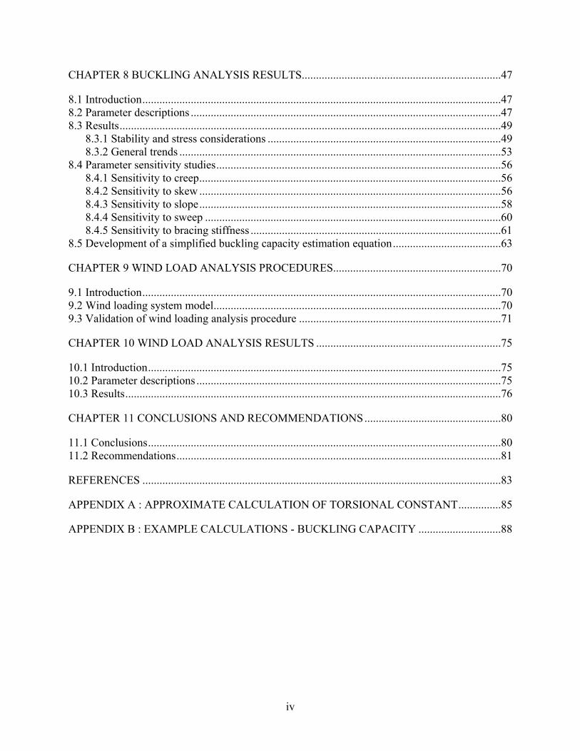
CHAPTER 8 BUCKLING ANALYSIS RESULTS......................................................................47
8.1 Introduction..............................................................................................................................47 8.2 Parameter descriptions .............................................................................................................47 8.3 Results......................................................................................................................................49
8.3.1 Stability and stress considerations ..................................................................................49 8.3.2 General trends .................................................................................................................53
8.4 Parameter sensitivity studies....................................................................................................56 8.4.1 Sensitivity to creep..........................................................................................................56 8.4.2 Sensitivity to skew ..........................................................................................................56 8.4.3 Sensitivity to slope..........................................................................................................58 8.4.4 Sensitivity to sweep ........................................................................................................60 8.4.5 Sensitivity to bracing stiffness ........................................................................................61
8.5 Development of a simplified buckling capacity estimation equation......................................63
CHAPTER 9 WIND LOAD ANALYSIS PROCEDURES...........................................................70
9.1 Introduction..............................................................................................................................70 9.2 Wind loading system model.....................................................................................................70 9.3 Validation of wind loading analysis procedure .......................................................................71
CHAPTER 10 WIND LOAD ANALYSIS RESULTS .................................................................75
10.1 Introduction............................................................................................................................75 10.2 Parameter descriptions ...........................................................................................................75 10.3 Results....................................................................................................................................76
CHAPTER 11 CONCLUSIONS AND RECOMMENDATIONS................................................80
11.1 Conclusions............................................................................................................................80 11.2 Recommendations..................................................................................................................81
REFERENCES ..............................................................................................................................83
APPENDIX A : APPROXIMATE CALCULATION OF TORSIONAL CONSTANT...............85
APPENDIX B : EXAMPLE CALCULATIONS - BUCKLING CAPACITY .............................88
1
CHAPTER 1 INTRODUCTION
1.1 Introduction
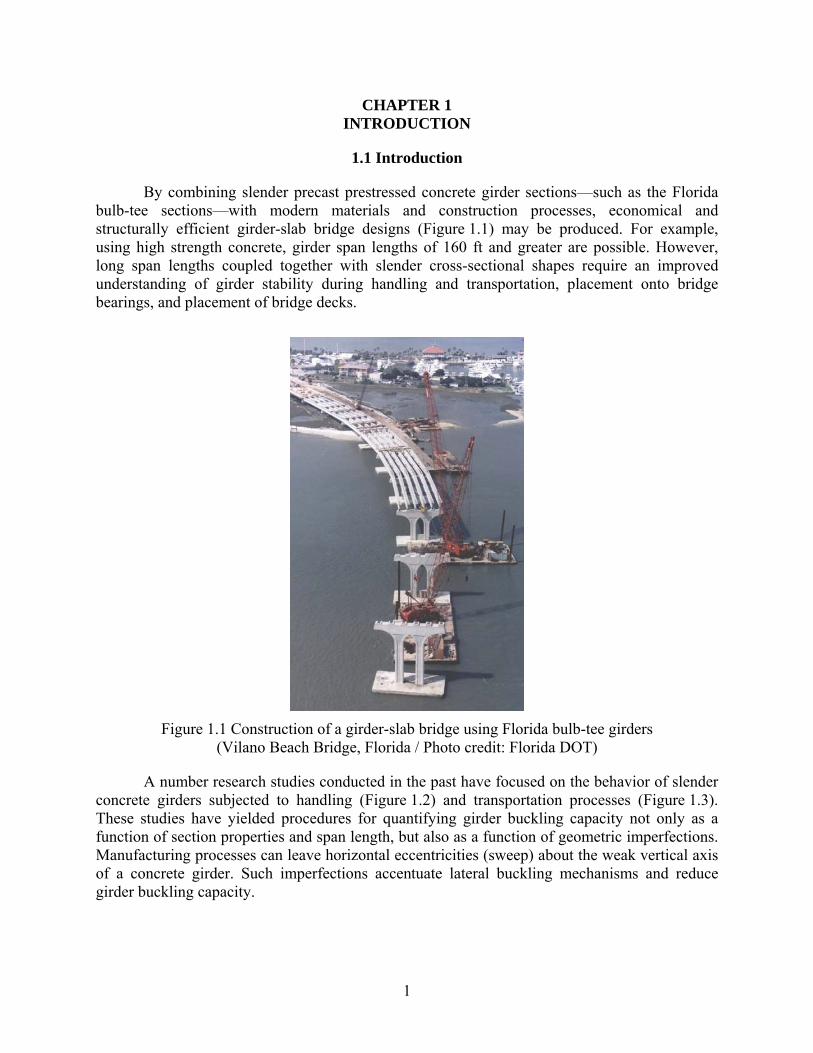
By combining slender precast prestressed concrete girder sections—such as the Florida bulb-tee sections—with modern materials and construction processes, economical and structurally efficient girder-slab bridge designs (Figure 1.1) may be produced. For example, using high strength concrete, girder span lengths of 160 ft and greater are possible. However, long span lengths coupled together with slender cross-sectional shapes require an improved understanding of girder stability during handling and transportation, placement onto bridge bearings, and placement of bridge decks.
Figure 1.1 Construction of a girder-slab bridge using Florida bulb-tee girders
(Vilano Beach Bridge, Florida / Photo credit: Florida DOT)
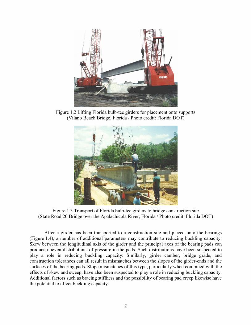
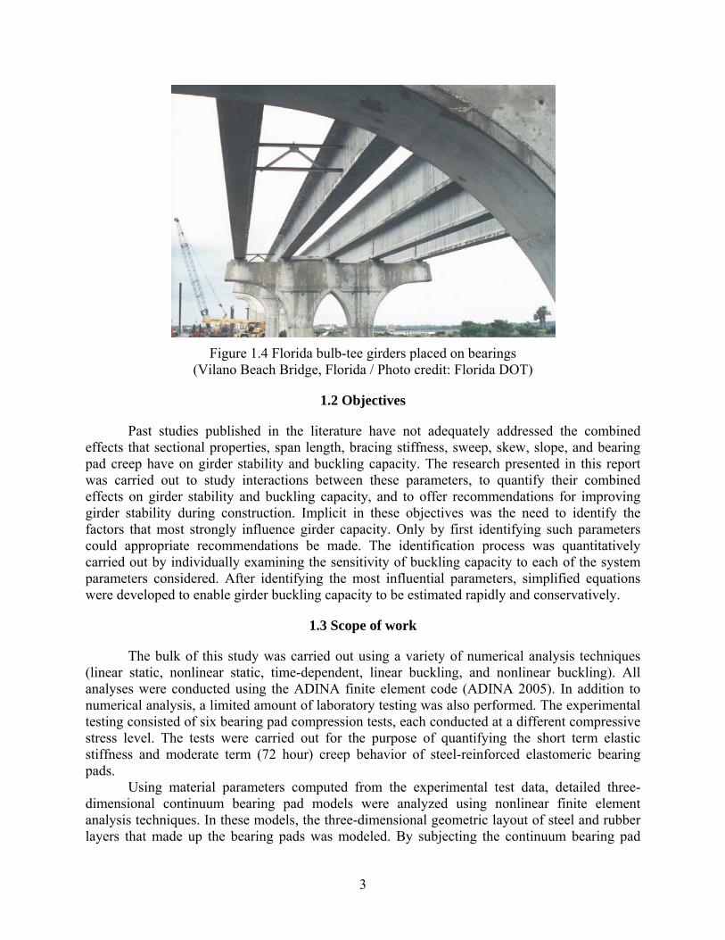
A number research studies conducted in the past have focused on the behavior of slender concrete girders subjected to handling (Figure 1.2) and transportation processes (Figure 1.3). These studies have yielded procedures for quantifying girder buckling capacity not only as a function of section properties and span length, but also as a function of geometric imperfections. Manufacturing processes can leave horizontal eccentricities (sweep) about the weak vertical axis of a concrete girder. Such imperfections accentuate lateral buckling mechanisms and reduce girder buckling capacity.
2
Figure 1.2 Lifting Florida bulb-tee girders for placement onto supports
(Vilano Beach Bridge, Florida / Photo credit: Florida DOT)
Figure 1.3 Transport of Florida bulb-tee girders to bridge construction site
(State Road 20 Bridge over the Apalachicola River, Florida / Photo credit: Florida DOT)
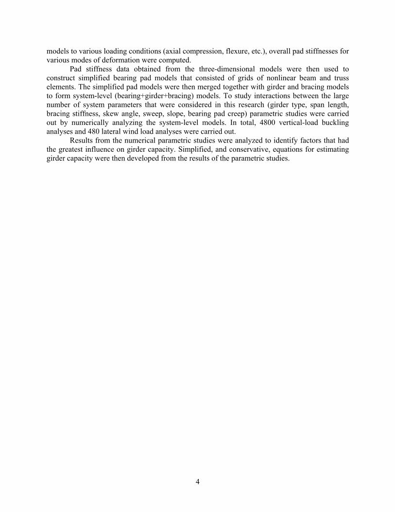
After a girder has been transported to a construction site and placed onto the bearings
(Figure 1.4), a number of additional parameters may contribute to reducing buckling capacity. Skew between the longitudinal axis of the girder and the principal axes of the bearing pads can produce uneven distributions of pressure in the pads. Such distributions have been suspected to play a role in reducing buckling capacity. Similarly, girder camber, bridge grade, and construction tolerances can all result in mismatches between the slopes of the girder-ends and the surfaces of the bearing pads. Slope mismatches of this type, particularly when combined with the effects of skew and sweep, have also been suspected to play a role in reducing buckling capacity. Additional factors such as bracing stiffness and the possibility of bearing pad creep likewise have the potential to affect buckling capacity.
3
Figure 1.4 Florida bulb-tee girders placed on bearings
(Vilano Beach Bridge, Florida / Photo credit: Florida DOT)
1.2 Objectives
Past studies published in the literature have not adequately addressed the combined effects that sectional properties, span length, bracing stiffness, sweep, skew, slope, and bearing pad creep have on girder stability and buckling capacity. The research presented in this report was carried out to study interactions between these parameters, to quantify their combined effects on girder stability and buckling capacity, and to offer recommendations for improving girder stability during construction. Implicit in these objectives was the need to identify the factors that most strongly influence girder capacity. Only by first identifying such parameters could appropriate recommendations be made. The identification process was quantitatively carried out by individually examining the sensitivity of buckling capacity to each of the system parameters considered. After identifying the most influential parameters, simplified equations were developed to enable girder buckling capacity to be estimated rapidly and conservatively.
1.3 Scope of work
The bulk of this study was carried out using a variety of numerical analysis techniques (linear static, nonlinear static, time-dependent, linear buckling, and nonlinear buckling). All analyses were conducted using the ADINA finite element code (ADINA 2005). In addition to numerical analysis, a limited amount of laboratory testing was also performed. The experimental testing consisted of six bearing pad compression tests, each conducted at a different compressive stress level. The tests were carried out for the purpose of quantifying the short term elastic stiffness and moderate term (72 hour) creep behavior of steel-reinforced elastomeric bearing pads.
Using material parameters computed from the experimental test data, detailed three-dimensional continuum bearing pad models were analyzed using nonlinear finite element analysis techniques. In these models, the three-dimensional geometric layout of steel and rubber layers that made up the bearing pads was modeled. By subjecting the continuum bearing pad
4
models to various loading conditions (axial compression, flexure, etc.), overall pad stiffnesses for various modes of deformation were computed.
Pad stiffness data obtained from the three-dimensional models were then used to construct simplified bearing pad models that consisted of grids of nonlinear beam and truss elements. The simplified pad models were then merged together with girder and bracing models to form system-level (bearing+girder+bracing) models. To study interactions between the large number of system parameters that were considered in this research (girder type, span length, bracing stiffness, skew angle, sweep, slope, bearing pad creep) parametric studies were carried out by numerically analyzing the system-level models. In total, 4800 vertical-load buckling analyses and 480 lateral wind load analyses were carried out.
Results from the numerical parametric studies were analyzed to identify factors that had the greatest influence on girder capacity. Simplified, and conservative, equations for estimating girder capacity were then developed from the results of the parametric studies.

5
CHAPTER 2 BACKGROUND
2.1 Literature review
Girder stability during the stages of girder production, handing, and transportation, has drawn the interest of a number of researchers in the past. Muller (1962) presented a method for computing the critical uniform vertical load for beams with typical types of end section conditions:
ycr 1 23
EI GJw = m k k
L (2.1)
In this equation, m is a variable coefficient dependent principally upon the end section conditions, crw is the critical buckling uniform load (also referred to as the “buckling capacity” in this report), yI is the moment of inertia about the weak vertical axis of the girder, J is the torsional constant, E is the elastic (Young’s) modulus of concrete, G is shear modulus of concrete, and L is the span length of the beam. If the ends of the beam are restrained, the influence of the shape of the cross section on buckling loads may be considered by introducing the coefficient k2 which takes into account additional restraint to lateral deflections of the top and bottom flanges. For loads applied at an eccentricity relative to the centroid of the section, the buckling load may be corrected by using a factor k1.
Regarding systems for bracing long span girders against buckling, George Laszlo and Richard Imper (1987) pointed out the limitations of a system known as king post bracing system. They noted that beyond a certain horizontal deflection of the beam, the system is useless and cannot prevent collapse of the beam. During shipping, impact forces and super-elevation may cause severe stress conditions due to weak axis bending moments. The combination of stresses resulting from prestress and lateral bending moment can lead to compression or cracking failure. To reduce the high tensile stresses, Laszlo and Imper suggested using supplementary reinforcing bars near the outer edges of the top flange if the induced stresses are below the cracking limit, and using temporary post-tensioning at the top flange if the stresses are above the allowable cracking limit. These methods, together with the use of higher strength concrete, are shown to be effective in preventing section cracking and improving beam stability. Suggested procedures for checking the stability of long span prestressed concrete beams against cracking are also given by Laszlo and Imper.
Mast (1993) focused on the stability of beams on elastic supports. Such supports include bearing pads and transportation equipment. It was found that rollover of beams supported from below is determined primarily by the properties of the support rather than of the beam. Long span prestressed concrete beams—when supported from below—were typically found to have adequate section stiffness but less roll-angle stiffness as provided by the flexible supports. Due to support flexibility, long span beams can roll sideways, resulting in lateral deflections that can lead to lateral instability. Because concrete beams normally have torsional stiffnesses that are much higher than the roll stiffnesses of the supports, Mast suggested that beams can be assumed to be rigid in torsion. This assumption transforms the problem into a bending and equilibrium
6
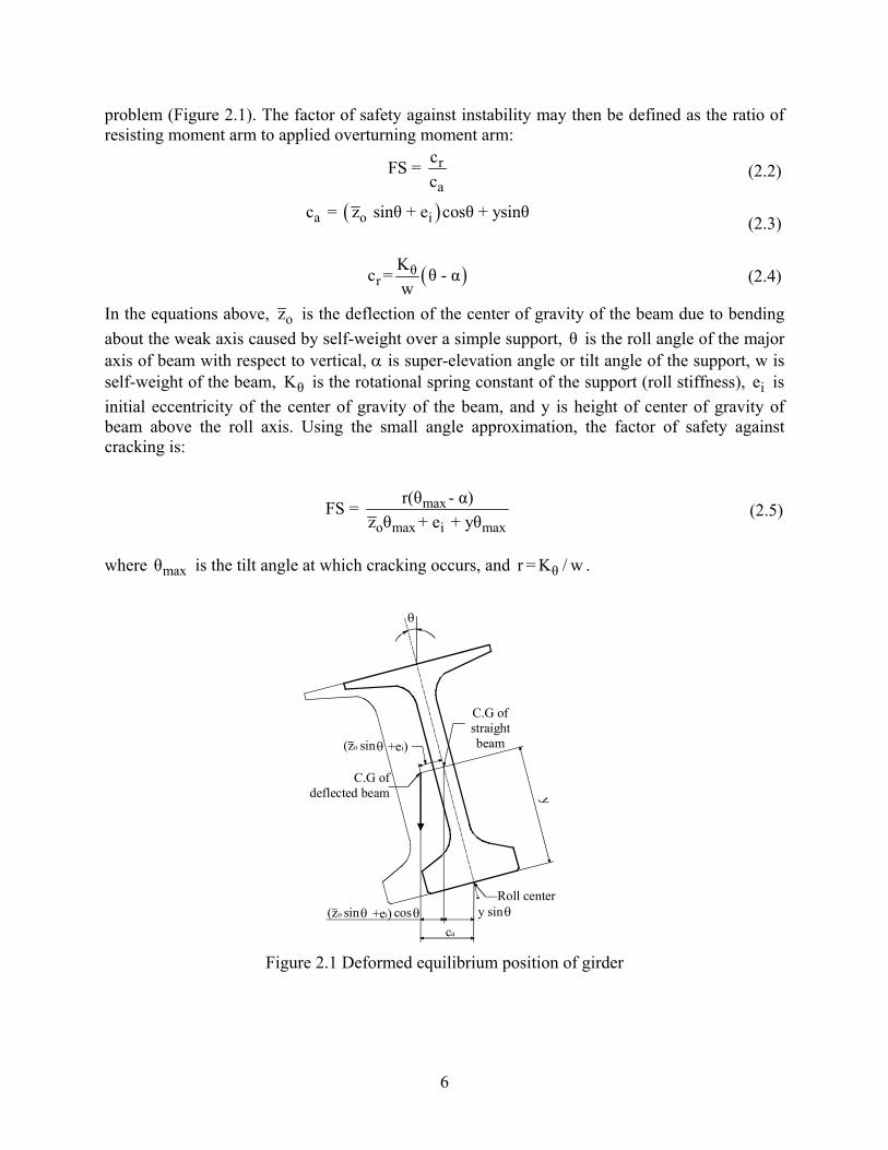
problem (Figure 2.1). The factor of safety against instability may then be defined as the ratio of resisting moment arm to applied overturning moment arm:
r
a
cFS = c
(2.2)
( )a o ic = z sinθ + e cosθ + ysinθ (2.3)
( )θr
Kc = θ - αw
(2.4)
In the equations above, oz is the deflection of the center of gravity of the beam due to bending about the weak axis caused by self-weight over a simple support, θ is the roll angle of the major axis of beam with respect to vertical, α is super-elevation angle or tilt angle of the support, w is self-weight of the beam, θK is the rotational spring constant of the support (roll stiffness), ie is initial eccentricity of the center of gravity of the beam, and y is height of center of gravity of beam above the roll axis. Using the small angle approximation, the factor of safety against cracking is:
where maxθ is the tilt angle at which cracking occurs, and θr = K / w .
y sinθcos θ(zo sinθ +ei)ca
(zo sinθ +ei)
y
θ
C.G of straight beam
C.G of deflected beam
Roll center
Figure 2.1 Deformed equilibrium position of girder
max
o max i max
r(θ - α)FS = z θ + e + yθ
(2.5)
7
Lateral stiffness decreases attributable to cracking at various tilt angles was also analyzed by Mast. Based on analysis results, Mast proposed a simplified relationship for the effective lateral stiffness of long prestressed concrete beams of ordinary proportions (e.g., the PCI bulb-tee
BT-72). When tilt angles θ produce top flange tensile stresses in excess of 'c7.5 f , the effective
minor axis cracked section moment of inertia is:
where θ is in units of radians. By analyzing the applied moment arm and resisting moment arm versus tilt angles for the PCI BT-72 section, on bearing pads having dimensions of 12 x 22 x 11/2 in., Mast (1993) showed that serious stability problems arise when using plain pads of this thickness. However, even with laminated pads, which appear to provide adequate stability, the angle required to cause instability is far less than the angle required to cause flange cracking, as was confirmed by full-scale testing (Mast 1994). Under wind load, long beams on bearing pads are susceptible to rolling sideways even with laminated pads. This emphasizes the effectiveness of bracing the ends of beams against rollover as soon as they are erected. When beams are set on elastomeric bearing pads, it is important that the weight of the beam be concentric on the pad. Eccentricity may cause rollover in extreme circumstances. Mast also suggested that for short-term activities, bearing pad creep effects can be neglected as long as the beams are not left in a tilted position for an extended period duration of time.
Procedures for evaluating the lateral stability of long prestressed concrete beams supported from below by using moment arm versus tilt angle relationships can also applied to the analysis of hanging beams (i.e., beams supported from above). The factor of safety against cracking for a hanging beam is given by:
Stratford and Burgoyne (1999) used finite element analysis to investigate the behavior of long prestressed concrete beams for three different types of support conditions: 1) simply supported at both ends; 2) supported as for transportation with one end supported against displacement but not rotation; and 3) hanging from support cables. Buckling analyses were performed for geometrically perfect beams (i.e., without sweep imperfections). The buckling loads computed agreed well with results reported by Trahair (1977, 1993) who derived expressions of the general form:
In this equation, k is a factor that depends on support conditions, L is the span length of beam, yI is the moment of inertia about the weak axis of the beam, J is the torsional constant, E is
elastic modulus of concrete, G is shear modulus of concrete, and wC is the warping constant.
g
effI
I =1 + 2.5θ
(2.6)
o r i max
1FS = z /y + θ /θ
(2.7)
2
y w 2
cr 3
πEI GJ + ECL
w = k πL
⎛ ⎞⎜ ⎟⎜ ⎟⎝ ⎠ (2.8)
8
Variations of computed buckling loads for hanging beams with different support cable angles, support heights, and lifting positions were investigated by Stratford and Burgoyne. Comparisons of buckling loads for the three different classes of support conditions cited above indicated that hanging beams are the most vulnerable to buckling. This is due to lack of torsional restraint about the longitudinal axis of the beam, allowing the beam to rotate until it finds an equilibrium position. Providing external torsional resistance therefore increases beam stability because the torsional rigidity of the beam itself is mobilized in preventing buckling.
Stratford and Burgoyne also developed nonlinear finite element models to investigate the load-deflection behaviors of beams with initial imperfections. Plots of results showed the nonlinear finite element analyses to be asymptotic to the line predicted by Allen and Bulson (1980):
In this equation, y is lateral deflection, 0y is the initial lateral (sweep) imperfection, w is the applied vertical uniform load, and crw is the critical uniform buckling load (i.e., the buckling capacity). Once the minor axis deflection has been computed, the twist of the beam at mid-span can be determined from:
where, by is the distance from the bottom fiber of the beam to the beam centroid, msy is the lateral beam deflection at mid-span, and δθ is the twist of the beam at mid-span. Twist angles can then be used to determine minor axis curvature and minor axis bending stresses as:
In the equation above, X is the lateral (perpendicular) distance from the weak axis to the point of interest. Stratford and Burgoyne (2001) also determined a relationship between the self-weight at which the beam would become unstable and the rotational stiffness of the bearing. They showed how the effects of initial imperfections in the beam will produce minor-axis curvature and hence additional stresses that can cause loss of stiffness due to cracking and subsequent beam failure. They proposed a method for computing buckling loads (capacities) of beams on flexible bearings under vertical loading. Assuming that the beam rotates as a rigid body—due to the high torsional stiffness of the concrete section—and using equilibrium, they proposed that the critical buckling load may obtained by solving:
( )o
2cr
yy = 1 - w/w
(2.9)
For simply supported beams: yms
E Iπδθ = yL G J
(2.10)
For transport supported beams: ( )1.68
0.36 /ms
y b
yL GJ EI y
δθ =− −
(2.11)
2
ms y
wL sin(δθ)κ = 8EI
(2.12)
msΔσ = E κ X (2.13)

9
for crw . In this equation, K is the rotational stiffness of the bearing. For beams with initial imperfections, the minor axis curvature of the beam versus the factor of safety ( crw /w ) can be found from:
where, 0v is initial lateral sweep imperfection. From the curvature at mid-span, msκ , stresses due to minor axis bending can be determined.
Lateral buckling of steel beams and the effectiveness of bracing such beams against lateral buckling are additional areas that have been investigated by past researchers. Although aspects of long span prestressed concrete beam buckling differ from steel beam behavior in many respects, literature dealing with lateral buckling of steel beams still provides useful insights into slender-beam behavior in general.
Flint (1951) studied the effect of intermediate, elastic restraints on the lateral buckling of steel beams. Simply supported beams braced at mid-span and loaded by either equal end moments or by a central load were analyzed. It was shown that the buckling capacity of a slender beam subjected solely to vertical load can be greatly enhanced by providing suitable bracing. Even with low stiffness, restraint of intermediate displacements can raise the critical buckling load sufficiently that the possibility of failure by elastic buckling is excluded. For the case of a beam with mid-span lateral restraint only, Flint proposed a simple design relationship between the increase in critical load and the lateral central support stiffness:
In this equation, c is ratio of critical buckling load with bracing to critical buckling load without bracing, and 3
B yλ = K L 48EI is the ratio of lateral restraint stiffness to lateral bending stiffness of the beam. Schmidt (1965) extended the work of Flint by studying the effects of interaction between elastic end torsional restraint and elastic central lateral restraint.
( )32
cr cr by
Lw L + w Ly - 2K = 0120EI
(2.14)
( )o
ms 2cr
48v 1κ =w /w - 15L
⎛ ⎞⎜ ⎟⎝ ⎠
(2.15)
c = 1+λ (2.16)

10
CHAPTER 3 DESCRIPTION OF PHYSICAL SYSTEM
3.1 Introduction
The physical system considered in this study consisted of a simple-span Florida bulb-tee girder supported on steel-reinforced elastomeric bearing pads (Figure 3.1). In most of the cases that were analyzed, end-point lateral bracing was considered, although unbraced conditions were also studied. Loading conditions for girder capacity calculations consisted of either uniform vertical (gravity) load or horizontal wind load.
Girder
BracingBearing pad
Support
Girder
Bracing
Support
Bearingpad
Uniform verticalload
Horizontal windpressure
(omitted in unbraced cases)
Figure 3.1 Schematic diagram of physical system and loading conditions
3.2 Terminology relating to geometric parameters
In Figure 3.1, the girder shown is geometrically perfect (no sweep, no camber, etc.), rests uniformly on the underling bearings pads, and is oriented at right angles to the pads. Realistic field conditions however, do not generally match such ideal conditions. Instead, girder imperfections (e.g., sweep) may exist, and the girder may not rest uniformly on—or at right angles to—the bearing pads. The vast majority of the cases considered in this study involved one or more of these non-ideal conditions. In order to make clear the types of geometric conditions that were considered, the following definitions and conventions are introduced:
11
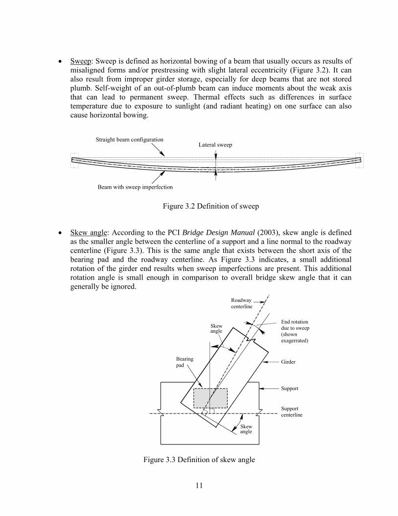
• Sweep: Sweep is defined as horizontal bowing of a beam that usually occurs as results of
misaligned forms and/or prestressing with slight lateral eccentricity (Figure 3.2). It can also result from improper girder storage, especially for deep beams that are not stored plumb. Self-weight of an out-of-plumb beam can induce moments about the weak axis that can lead to permanent sweep. Thermal effects such as differences in surface temperature due to exposure to sunlight (and radiant heating) on one surface can also cause horizontal bowing.
Straight beam configuration
Beam with sweep imperfection
Lateral sweep
Figure 3.2 Definition of sweep
• Skew angle: According to the PCI Bridge Design Manual (2003), skew angle is defined as the smaller angle between the centerline of a support and a line normal to the roadway centerline (Figure 3.3). This is the same angle that exists between the short axis of the bearing pad and the roadway centerline. As Figure 3.3 indicates, a small additional rotation of the girder end results when sweep imperfections are present. This additional rotation angle is small enough in comparison to overall bridge skew angle that it can generally be ignored.
Girder
Skewangle
End rotation due to sweep(shown exagerrated)
Roadwaycenterline
Support
Skewangle
Support centerline
Bearingpad
Figure 3.3 Definition of skew angle

12
• Slope angle: Slope angle is defined as the vertical angle between the girder axis at the support and a horizontal line level with the surface of the bearing pad. Slope angles may be produced by camber—induced by eccentric prestressing of the girder—or by overall bridge grade. In this study, slope angle is defined as the slope mismatch (gap) that exists between the bottom face of the girder and the top face of the bearing pad.
Support
Slopeangle
Bearing pad
Girder
Figure 3.4 Definition of slope angle
3.3 Bearing pads
Bearings are used to transfer loads from the superstructure to the substructure and to allow translational and rotational movements of the superstructure that may arise from vehicle loads and environmental loads such as thermal expansion and contraction. Various types of bearings are used for bridges including: elastomeric bearings, pot bearings, rocker bearings, cylindrical bearings, spherical bearings, and roller bearings. Each type of bearing has different translational and rotational stiffnesses, to accommodate appropriate movements of the bridge, and therefore creates different boundary conditions for the girders.
Elastomeric bearings provide an efficient and economical solution to the problem of supporting girders vertically while also permitting horizontal thermal movements. Elastomeric bearings are generally categorized into one of four main types: plain elastomeric pads, fiberglass reinforced elastomeric pads, steel reinforced elastomeric pads, and cotton duck reinforced elastomeric pads. Of these types, steel reinforced elastomeric pads are used extensively for bridge beam support in the state of Florida and throughout the country. The Florida Department of Transportation (FDOT) suggests the use of elastomeric bearings for simple span, prestressed concrete beam, simple-span steel girder and some continuous beams. Therefore, steel reinforced elastomeric bearings are the only type of bearings considered in this study.
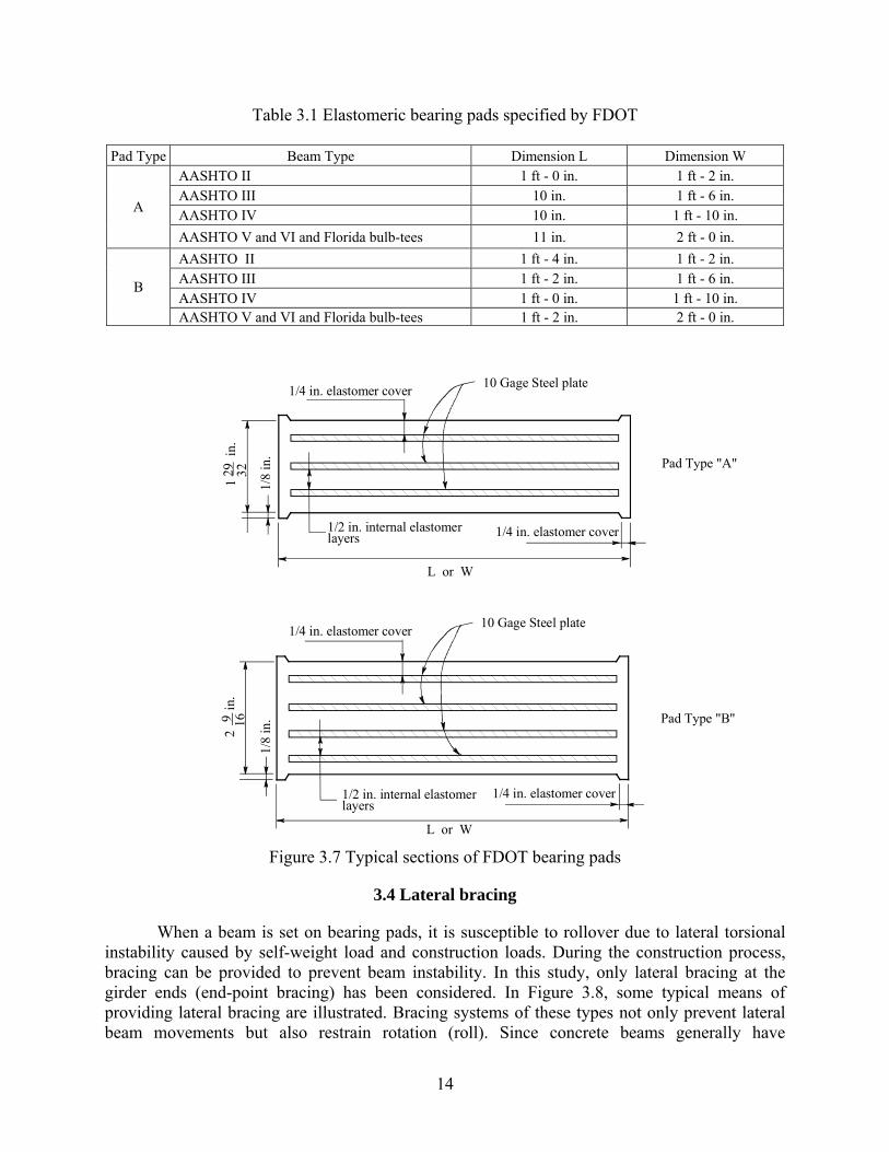
Steel-reinforced elastomeric bearing pads consist of multiple layers of elastomeric material bonded to steel shims in a sandwich form (Figure 3.5). Steel shims enhance the compression capacity of the bearing pad by restraining lateral bulging of the elastomeric layers. However, the steel shims do not inhibit the shear flexibility of the pad which is needed to accommodate bridge movements in the horizontal direction. The various behavioral modes of pad deformation that are relevant to the current research are presented in Figure 3.6.
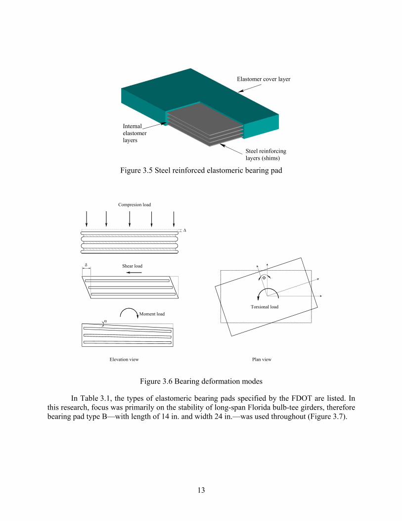
13
Steel reinforcinglayers (shims)
Elastomer cover layer
Internal elastomer layers
Figure 3.5 Steel reinforced elastomeric bearing pad
Compresion load
Δ
Shear loadδ
Moment loadα
Torsional load
Φ
Elevation view Plan view
Figure 3.6 Bearing deformation modes
In Table 3.1, the types of elastomeric bearing pads specified by the FDOT are listed. In this research, focus was primarily on the stability of long-span Florida bulb-tee girders, therefore bearing pad type B—with length of 14 in. and width 24 in.—was used throughout (Figure 3.7).
14
Table 3.1 Elastomeric bearing pads specified by FDOT
Pad Type Beam Type Dimension L Dimension W AASHTO II 1 ft - 0 in. 1 ft - 2 in. AASHTO III 10 in. 1 ft - 6 in. AASHTO IV 10 in. 1 ft - 10 in. A
AASHTO V and VI and Florida bulb-tees 11 in. 2 ft - 0 in. AASHTO II 1 ft - 4 in. 1 ft - 2 in. AASHTO III 1 ft - 2 in. 1 ft - 6 in. AASHTO IV 1 ft - 0 in. 1 ft - 10 in.
B
AASHTO V and VI and Florida bulb-tees 1 ft - 2 in. 2 ft - 0 in.
1/8
in.
1
in
.29 32
1/4 in. elastomer cover 10 Gage Steel plate
1/4 in. elastomer cover
L or W
1/2 in. internal elastomer layers
1/8
in.
2
in.
9 16
1/4 in. elastomer cover 10 Gage Steel plate
1/4 in. elastomer cover
L or W
1/2 in. internal elastomer layers
Pad Type "A"
Pad Type "B"
Figure 3.7 Typical sections of FDOT bearing pads
3.4 Lateral bracing
When a beam is set on bearing pads, it is susceptible to rollover due to lateral torsional instability caused by self-weight load and construction loads. During the construction process, bracing can be provided to prevent beam instability. In this study, only lateral bracing at the girder ends (end-point bracing) has been considered. In Figure 3.8, some typical means of providing lateral bracing are illustrated. Bracing systems of these types not only prevent lateral beam movements but also restrain rotation (roll). Since concrete beams generally have
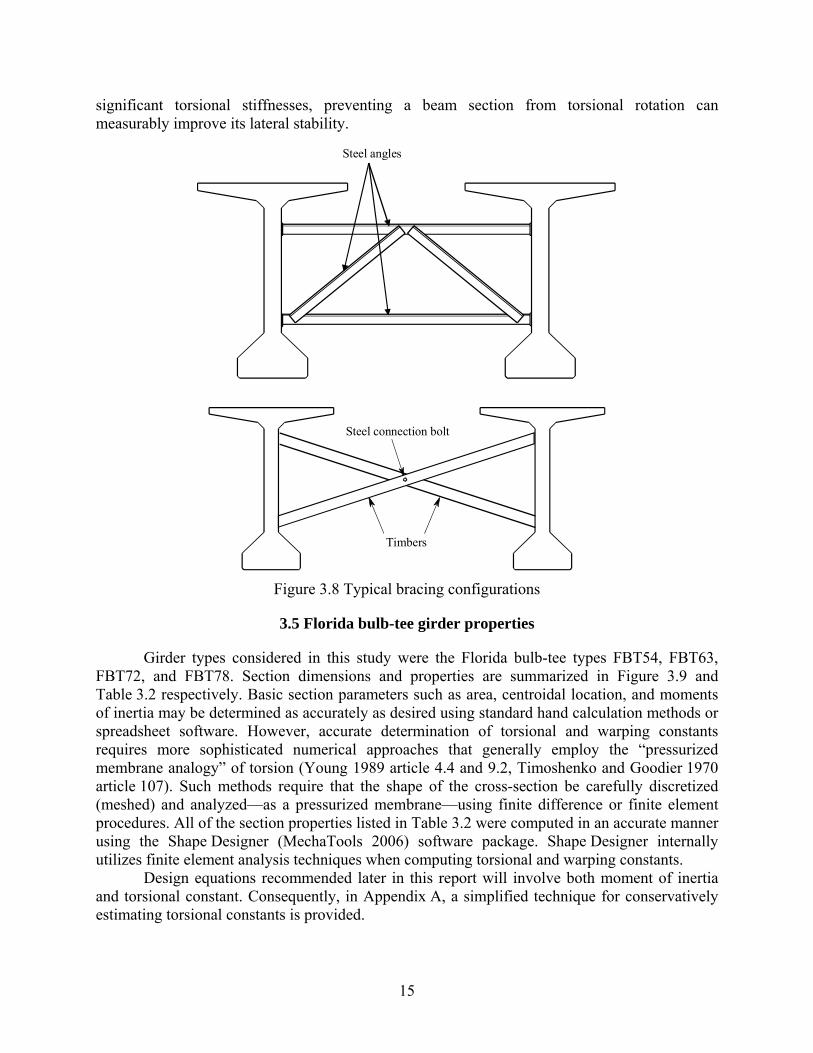
15
significant torsional stiffnesses, preventing a beam section from torsional rotation can measurably improve its lateral stability.
Timbers
Steel connection bolt
Steel angles
Figure 3.8 Typical bracing configurations
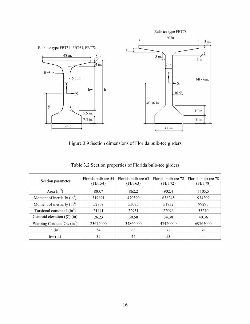
3.5 Florida bulb-tee girder properties
Girder types considered in this study were the Florida bulb-tee types FBT54, FBT63, FBT72, and FBT78. Section dimensions and properties are summarized in Figure 3.9 and Table 3.2 respectively. Basic section parameters such as area, centroidal location, and moments of inertia may be determined as accurately as desired using standard hand calculation methods or spreadsheet software. However, accurate determination of torsional and warping constants requires more sophisticated numerical approaches that generally employ the “pressurized membrane analogy” of torsion (Young 1989 article 4.4 and 9.2, Timoshenko and Goodier 1970 article 107). Such methods require that the shape of the cross-section be carefully discretized (meshed) and analyzed—as a pressurized membrane—using finite difference or finite element procedures. All of the section properties listed in Table 3.2 were computed in an accurate manner using the Shape Designer (MechaTools 2006) software package. Shape Designer internally utilizes finite element analysis techniques when computing torsional and warping constants.
Design equations recommended later in this report will involve both moment of inertia and torsional constant. Consequently, in Appendix A, a simplified technique for conservatively estimating torsional constants is provided.
16
30 in.
48 in.
6.5 in.R=8 in.
X
Y X
Y
10.5"
5.5 in.
y_
7.5 in.
2 in.
4 in.
hw h
8 in.
10 in.
6ft - 6in.
3 in.
3 in.60 in.
7 in.
3 in.4 in.
40.36 in.
28 in.
Bulb-tee type FBT54, FBT63, FBT72
Bulb-tee type FBT78
Figure 3.9 Section dimensions of Florida bulb-tee girders
Table 3.2 Section properties of Florida bulb-tee girders
Section parameter Florida bulb-tee 54 (FBT54)
Florida bulb-tee 63(FBT63)
Florida bulb-tee 72 (FBT72)
Florida bulb-tee 78(FBT78)
Area (in2) 803.7 862.2 902.4 1105.5 Moment of inertia Ix (in4) 319691 470390 638245 934209 Moment of inertia Iy (in4) 52869 53075 51832 99295 Torsional constant J (in4) 21441 22931 22096 35270
Centroid elevation ( y ) (in) 26.23 30.50 34.30 40.36 Warping Constant Cw (in6) 23674000 34866000 47420000 69765000
h (in) 54 63 72 78 hw (in) 35 44 53 —
17
CHAPTER 4 EXPERIMENTAL TESTING OF BEARING PADS
4.1 Introduction
Boundary conditions relating to rotational and translational restraint, effective at the ends of a girder, have significant influence on stability against buckling. While idealized boundary conditions may be classified as either fixed (full restraint) or free (zero restraint), actual boundary conditions in the field lie between the fixed and free limiting conditions. Specific levels of rotational and translational fixity are direct functions of the stiffness of the bearing pads upon which the ends of a girder rest. Immediately following girder placement, the short term elastic stiffness of the bearing pads is of primary importance. However, in this study, it was also of interest to determine whether longer term creep effects in bearing pads could have an effect on girder stability over a time period of a few days. Rather than relying strictly on bearing pad data available in the published literature, experimental tests were carried out to obtain short term (elastic) and moderate term (creep) material properties.
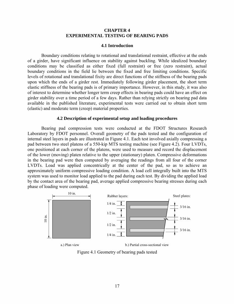
4.2 Description of experimental setup and loading procedures
Bearing pad compression tests were conducted at the FDOT Structures Research Laboratory by FDOT personnel. Overall geometry of the pads tested and the configuration of internal steel layers in pads are illustrated in Figure 4.1. Each test involved axially compressing a pad between two steel platens of a 550-kip MTS testing machine (see Figure 4.2). Four LVDTs, one positioned at each corner of the platens, were used to measure and record the displacement of the lower (moving) platen relative to the upper (stationary) platen. Compressive deformations in the bearing pad were then computed by averaging the readings from all four of the corner LVDTs. Load was applied concentrically at the center of the pad, so as to achieve an approximately uniform compressive loading condition. A load cell integrally built into the MTS system was used to monitor load applied to the pad during each test. By dividing the applied load by the contact area of the bearing pad, average applied compressive bearing stresses during each phase of loading were computed.
10 in.
10 in
.
Steel plates:
3/16 in.
3/16 in.
3/16 in.
1/4 in.
1/4 in.
1/2 in.
1/2 in.
Rubber layers:
a.) Plan view b.) Partial cross-sectional view Figure 4.1 Geometry of bearing pads tested

18
Upper (stationary) platen
Lower (moving) platenBearing pad
LVDTs (typical)
Figure 4.2 Experimental setup used to test bearing pads
Each test involved two phases of compressive loading: a short term elastic phase followed by a longer term creep phase. The short term elastic phase involved applying compressive load to the pad in a generally monotonically increasing manner until a target compressive stress level was achieved. This phase of loading was relatively short in length, generally lasting less than approximately 10 minutes in duration. Once the target compressive stress level on the pad was reached, a longer term creep phase commenced. Using an active feedback control system, a load-controlled, constant-stress condition was held on the pad for durations of up to approximately three days. During this time frame, constant-stress creep deformations in the pad were measured and recorded so that appropriate time-dependent material creep parameters could later be computed.
Tests were conducted at six different target compressive stress levels (see Table 4.1). Stresses near the low to middle range corresponded to typical stress levels induced by bridge dead loads acting on a bearing pad and making uniform contact across the entire contact area of the pad. Stresses near the upper end of the range corresponded to the much higher stresses that may occur in localized corners of a pad when combinations of skew and slope result in an initially small contact area between the girder and pad.
Table 4.1 Stress levels used in bearing pad tests
Test Applied compressive stress (psi)
Total test duration (hrs)
1 150 49 2 450 69 3 1500 71 4 3000 71 5 4000 52 6 4500 15*
* Pad failed under applied loading after 15 hrs of testing.
19
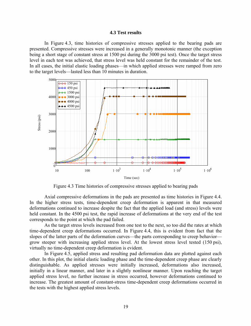
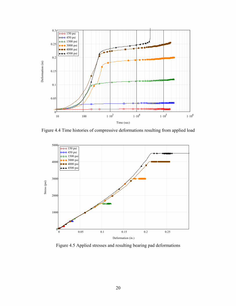
4.3 Test results
In Figure 4.3, time histories of compressive stresses applied to the bearing pads are presented. Compressive stresses were increased in a generally monotonic manner (the exception being a short stage of constant stress at 1500 psi during the 3000 psi test). Once the target stress level in each test was achieved, that stress level was held constant for the remainder of the test. In all cases, the initial elastic loading phases—in which applied stresses were ramped from zero to the target levels—lasted less than 10 minutes in duration.
10 100 1 .103 1 .104 1 .105 1 .1060
1000
2000
3000
4000
5000150 psi450 psi1500 psi3000 psi4000 psi4500 psi
Time (sec)
Stre
ss (p
si)
Figure 4.3 Time histories of compressive stresses applied to bearing pads
Axial compressive deformations in the pads are presented as time histories in Figure 4.4. In the higher stress tests, time-dependent creep deformation is apparent in that measured deformations continued to increase despite the fact that the applied load (and stress) levels were held constant. In the 4500 psi test, the rapid increase of deformations at the very end of the test corresponds to the point at which the pad failed.
As the target stress levels increased from one test to the next, so too did the rates at which time-dependent creep deformations occurred. In Figure 4.4, this is evident from fact that the slopes of the latter parts of the deformation curves—the parts corresponding to creep behavior—grow steeper with increasing applied stress level. At the lowest stress level tested (150 psi), virtually no time-dependent creep deformation is evident.
In Figure 4.5, applied stress and resulting pad deformation data are plotted against each other. In this plot, the initial elastic loading phase and the time-dependent creep phase are clearly distinguishable. As applied stresses were initially increased, deformations also increased, initially in a linear manner, and later in a slightly nonlinear manner. Upon reaching the target applied stress level, no further increase in stress occurred, however deformations continued to increase. The greatest amount of constant-stress time-dependent creep deformations occurred in the tests with the highest applied stress levels.
20
10 100 1 .103 1 .104 1 .105 1 .1060
0.05
0.1
0.15
0.2
0.25
0.3150 psi450 psi1500 psi3000 psi4000 psi 4500 psi
Time (sec)
Def
orm
atio
n (in
)
Figure 4.4 Time histories of compressive deformations resulting from applied load
0 0.05 0.1 0.15 0.2 0.250
1000
2000
3000
4000
5000150 psi450 psi1500 psi3000 psi4000 psi4500 psi
Deformation (in.)
Stre
ss (p
si)
Figure 4.5 Applied stresses and resulting bearing pad deformations
21
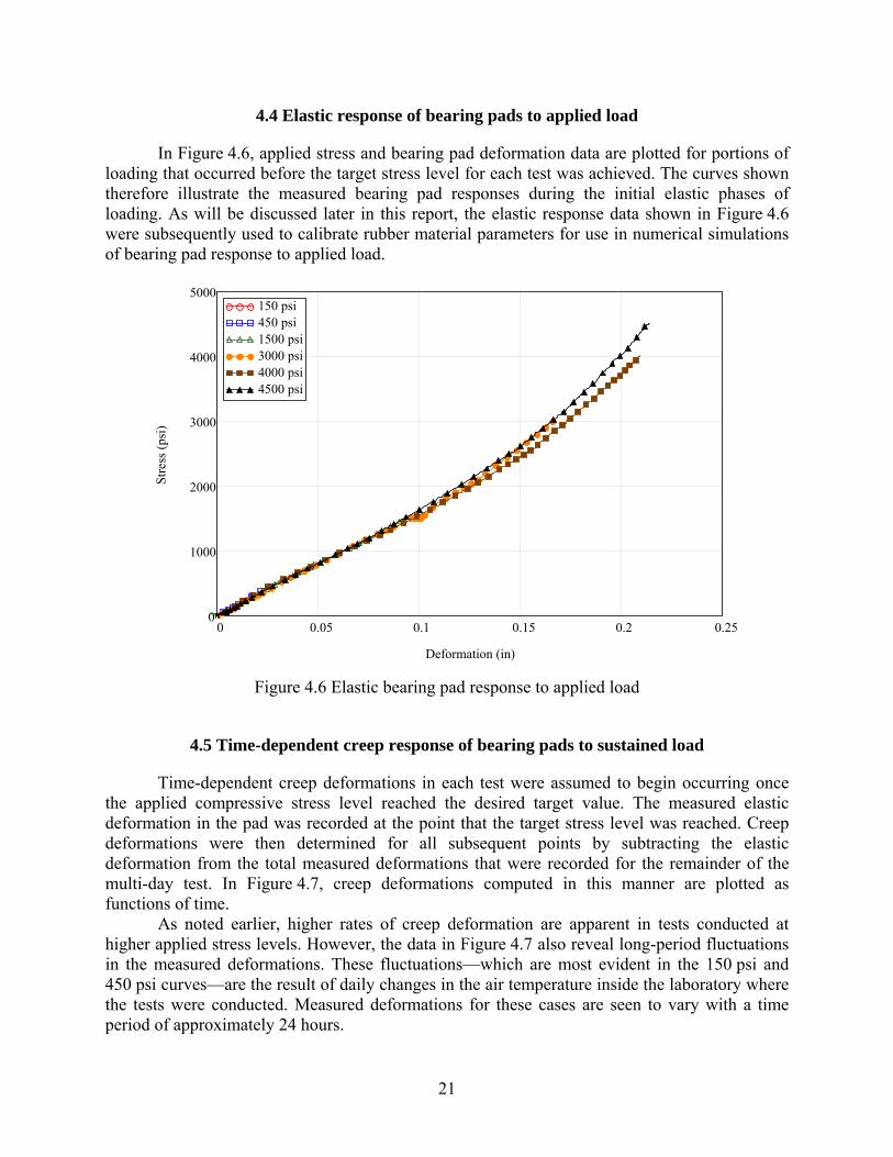
4.4 Elastic response of bearing pads to applied load
In Figure 4.6, applied stress and bearing pad deformation data are plotted for portions of loading that occurred before the target stress level for each test was achieved. The curves shown therefore illustrate the measured bearing pad responses during the initial elastic phases of loading. As will be discussed later in this report, the elastic response data shown in Figure 4.6 were subsequently used to calibrate rubber material parameters for use in numerical simulations of bearing pad response to applied load.
0 0.05 0.1 0.15 0.2 0.250
1000
2000
3000
4000
5000150 psi450 psi1500 psi3000 psi4000 psi4500 psi
Deformation (in)
Stre
ss (p
si)
Figure 4.6 Elastic bearing pad response to applied load
4.5 Time-dependent creep response of bearing pads to sustained load
Time-dependent creep deformations in each test were assumed to begin occurring once the applied compressive stress level reached the desired target value. The measured elastic deformation in the pad was recorded at the point that the target stress level was reached. Creep deformations were then determined for all subsequent points by subtracting the elastic deformation from the total measured deformations that were recorded for the remainder of the multi-day test. In Figure 4.7, creep deformations computed in this manner are plotted as functions of time.
As noted earlier, higher rates of creep deformation are apparent in tests conducted at higher applied stress levels. However, the data in Figure 4.7 also reveal long-period fluctuations in the measured deformations. These fluctuations—which are most evident in the 150 psi and 450 psi curves—are the result of daily changes in the air temperature inside the laboratory where the tests were conducted. Measured deformations for these cases are seen to vary with a time period of approximately 24 hours.
22
0 5 .104 1 .105 1.5 .105 2 .105 2.5 .105 3 .1050
0.01
0.02
0.03
0.04
0.05150 psi450 psi1500 psi3000 psi4000 psi4500 psi
Time (sec)
Cre
ep d
efor
mat
ion
(in)
Figure 4.7 Time histories of measured creep deformations
In Figure 4.8, the same data are plotted, except that the time scale has been plotted using a logarithmic scale instead of a linear scale. The overall slopes of the curves shown in Figure 4.8 are direct indicators of the rates at which time-dependent creep deformations occurred during each of the tests.
In order to perform numerical parametric analyses (discussed later in this report) that account for creep deformations, a simplified mathematical model of creep behavior was developed from the measured experimental data. The form of the creep model chosen for this study was the power creep law :
a a1 2c 0ε (t) = a σ t (4.1)
where coefficients 0a , 1a , and 2a are material parameters. In order to solve for the coefficients 0a , 1a , and 2a that best matched the power creep
law to the measured experimental data, a least squares curve fitting procedure was employed. Starting with the approximately 10,000 or so data points that were contained within each creep curve from the laboratory testing, a numerical procedure was used to resample the creep deformations at 200 quadratically-spaced points. Quadratic spacing—rather than equal (linear) spacing—was chosen so as to achieve a higher density of sampling points in the early portion of each creep data record where creep deformations changed most rapidly with respect to time. Values of creep strain were then computed from each of the resampled creep deformation values. The resulting time histories of creep strain are shown in Figure 4.9
23
1 10 100 1 .103 1 .104 1 .105 1 .1060
0.01
0.02
0.03
0.04
0.05150 psi450 psi1500 psi3000 psi4000 psi4500 psi
Time (sec)
Cre
ep d
efor
mat
ion
(in)
Figure 4.8 Time histories of measured creep deformations
0 5 .104 1 .105 1.5 .105 2 .105 2.5 .105 3 .1050
0.01
0.02
0.03
0.04150 psi450 psi1500 psi3000 psi4000 psi4500 psi
Time (sec)
Cre
ep st
rain
(in/
in)
Figure 4.9 Time histories of creep strains (Points are have been resampled quadratically along the time-scale)
24
Using data from each of the six (6) experimental tests and the two hundred (200) resampled points from each test, the following cumulative error function was formulated:
( ) ( ) ( )26 200 aa 21
0 1 2 c 0 i jtest i,ji=1 j=1
tests times
Error(a , a , a ) = ε a σ t⎛ ⎞−⎜ ⎟⎝ ⎠∑ ∑ (4.2)
where ctestε were the creep strain values determined from the experimental tests. A numerical
minimization process was then used to solve for the coefficients 0a , 1a , and 2a that minimized the error function given by Eqn. 4.2. The resulting values of the power creep law coefficients were:
0a = 0.00000857, 1a = 0.77924377, and 2a = 0.14772347
Using these values in Eqn. 4.1, power law creep curves were computed for each of the stress levels tested experimentally. Comparisons of the (resampled) experimental data and best-fit power law creep model are shown in Figure 4.10. The values of the coefficients 0a , 1a , and 2a given above were used throughout the rest of this study whenever creep effects were to be taken into account.
0 5 .104 1 .105 1.5 .105 2 .105 2.5 .105 3 .105 3.5 .105 4 .1050
0.01
0.02
0.03
0.04150 psi (experimental)450 psi (experimental)1500 psi (experimental)3000 psi (experimental)4000 psi (experimental)4500 psi (experimental)150 psi (power law)450 psi (power law)1500 psi (power law)3000 psi (power law)4000 psi (power law)4500 psi (power law)
Time (sec)
Cre
ep st
rain
(in/
in)
Figure 4.10 Comparison of experimental creep data and best-fit power creep law

25
CHAPTER 5 DETAILED 3D BEARING PAD MODELING
5.1 Bearing pad model
Assessing the stability of long-span girders supported on bearing pads required that pad behavior under various types of loading conditions and deformation patterns be numerically characterized. Pad stiffnesses for compression, torsion, shear, and moment (roll) at varying skew angles were determined by conducting three-dimensional (3D) finite element analyses. All such analyses were carried out using the ADINA nonlinear finite element code. As shown in Figure 5.1, the bearing pad model developed in this study consisted of multiple alternating layers of elastomer and steel and matched the configuration of the FDOT Type B elastomeric bearing pad. All materials (elastomer and steel) were modeled using 3D meshes of twenty-seven-node solid brick elements.
Physically, when steel plates are embedded within a pad, the overall compression stiffness of the pad is increased by reducing the levels of bulging that occur in the elastomeric layers. Achieving this outcome requires that shear stresses be transmitted across the bonded surfaces between the steel plates and elastomeric layers. In the finite element model, bond between steel and elastomer was assumed to be perfect and was therefore modeled by ensuring that the finite element meshes of the elastomeric layers and steel plates shared common nodes at their interfaces.
2 in.916
1/4 in. Elastomer cover
1/2 in. Internal Elastomer layers
10 gage steel plates
Z
X
Y
14 in.
24 in.
Figure 5.1 Three-dimensional finite element model of bearing pad
Steel plates were modeled using a linear elastic material model with an elastic (Young’s) modulus of 29,000 ksi and a Poisson’s ratio of 0.3. Elastomeric layers were modeled using the Ogden rubber material model. For this type of material model, ADINA uses a large-displacement and large-strain formulation for solid finite elements. For the Ogden material model, ADINA permits the user to represent the form of the strain energy density function by specifying up to 19 material coefficients: nμ and nα for n=1,2,…9, and a bulk modulus K. It was determined that the standard three-term Ogden material description nμ and nα for n=1,2,3, was suitable for use in modeling the elastomer elements. As such, six coefficients plus a bulk modulus were specified. The procedures used to determine these coefficients are discussed below.
26
5.2 Determination of material properties
Initially, coefficients of the elastomer (rubber) material model were obtained from published literature. The material coefficients presented below were developed from test data initially published by Treloar (1944). The tests consisted of a biaxial test, a simple elongation test, and a pure shear test. As presented by Gent (2001), the resulting material coefficients, are:
μ1 = 0.6180 MPa
μ2 = 0.001177 MPa μ3 = -0.009811 MPa
α1 = 1.3 α2 = 5.0 α3 = -2.0
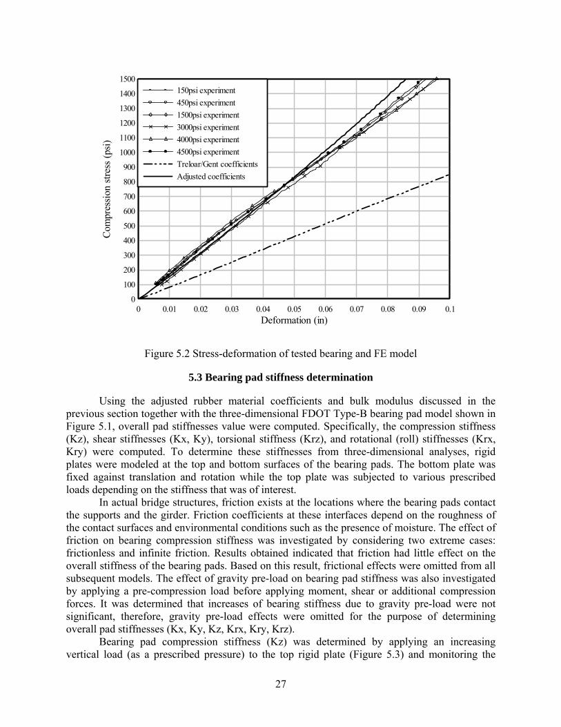
Determination of whether these values were appropriate for bearing pad modeling was carried out by numerically simulating the experimental compression tests presented in the previous chapter. A detailed three-dimensional model of the 10 in. x 10 in. x 2-1/16 in. bearing pads (with three steel shims) experimentally tested at the FDOT Structures Research Laboratory was constructed in a manner similar to that shown in Figure 5.1 for the FDOT Type B bearing pad. Using the material coefficients noted above to model the elastomeric layers, a compression test was simulated using the three-dimensional model. In Figure 5.2, the simulated (finite element) compression test results and the experimentally determined data are compared. It is evident from the figure that, using the Treloar/Gent material parameters, the compression stiffness of the bearing pad, as predicted by finite element analysis, is approximately one-half of that measured during the experiments.
Therefore, adjustments were made to the material coefficients to bring the compression behavior predicted by finite element analysis into agreement with the experimental test data. The adjusted material coefficients were:
μ1 = 0.6180 MPa
μ2 = 0.001177 MPa μ3 = -0.459811 MPa
α1 = 1.3 α2 = 5.0 α3 = -2.0
As Figure 5.2 indicates, compression behavior predicted using the adjusted coefficients and finite element analysis compares favorably to the experimental test data. The bulk modulus (K) used in the finite element simulations was set to 165 ksi, which was estimated based on data in the literature and using the formula:
2G(1+ν)K = 3(1-2ν)
(5.1)
In this equation, G is the small-strain shear modulus of the material, which can be written in terms of the other material coefficients as:
3
n nn=1
1G = μ α2 ∑ (5.2)
In Eqn. 5.1, Poisson’s ratio ν was set to 0.49962 to produce the bulk modulus value noted above. Also, note that ν is very close to 0.5 since the rubber used in bearing pads is a nearly incompressible material.
27
Deformation (in)
Com
pres
sion
stres
s (ps
i)
0 0.01 0.02 0.03 0.04 0.05 0.06 0.07 0.08 0.09 0.10
100
200
300
400
500
600
700
800
900
1000
1100
1200
1300
1400
1500150psi experiment450psi experiment1500psi experiment3000psi experiment4000psi experiment4500psi experimentTreloar/Gent coefficientsAdjusted coefficients
Figure 5.2 Stress-deformation of tested bearing and FE model
5.3 Bearing pad stiffness determination
Using the adjusted rubber material coefficients and bulk modulus discussed in the previous section together with the three-dimensional FDOT Type-B bearing pad model shown in Figure 5.1, overall pad stiffnesses value were computed. Specifically, the compression stiffness (Kz), shear stiffnesses (Kx, Ky), torsional stiffness (Krz), and rotational (roll) stiffnesses (Krx, Kry) were computed. To determine these stiffnesses from three-dimensional analyses, rigid plates were modeled at the top and bottom surfaces of the bearing pads. The bottom plate was fixed against translation and rotation while the top plate was subjected to various prescribed loads depending on the stiffness that was of interest.
In actual bridge structures, friction exists at the locations where the bearing pads contact the supports and the girder. Friction coefficients at these interfaces depend on the roughness of the contact surfaces and environmental conditions such as the presence of moisture. The effect of friction on bearing compression stiffness was investigated by considering two extreme cases: frictionless and infinite friction. Results obtained indicated that friction had little effect on the overall stiffness of the bearing pads. Based on this result, frictional effects were omitted from all subsequent models. The effect of gravity pre-load on bearing pad stiffness was also investigated by applying a pre-compression load before applying moment, shear or additional compression forces. It was determined that increases of bearing stiffness due to gravity pre-load were not significant, therefore, gravity pre-load effects were omitted for the purpose of determining overall pad stiffnesses (Kx, Ky, Kz, Krx, Kry, Krz).
Bearing pad compression stiffness (Kz) was determined by applying an increasing vertical load (as a prescribed pressure) to the top rigid plate (Figure 5.3) and monitoring the
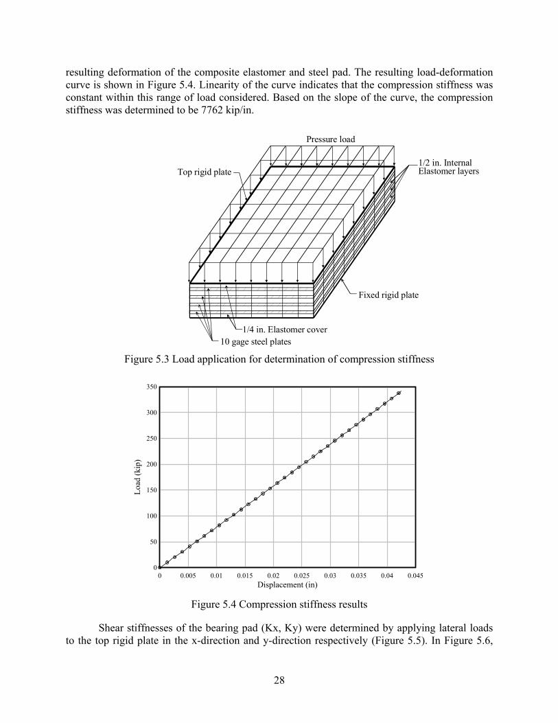
28
resulting deformation of the composite elastomer and steel pad. The resulting load-deformation curve is shown in Figure 5.4. Linearity of the curve indicates that the compression stiffness was constant within this range of load considered. Based on the slope of the curve, the compression stiffness was determined to be 7762 kip/in.
1/4 in. Elastomer cover10 gage steel plates
1/2 in. Internal Elastomer layers
Pressure load
Fixed rigid plate
Top rigid plate
Figure 5.3 Load application for determination of compression stiffness
Displacement (in)
Load
(kip
)
0 0.005 0.01 0.015 0.02 0.025 0.03 0.035 0.04 0.0450
50
100
150
200
250
300
350
Figure 5.4 Compression stiffness results
Shear stiffnesses of the bearing pad (Kx, Ky) were determined by applying lateral loads to the top rigid plate in the x-direction and y-direction respectively (Figure 5.5). In Figure 5.6,
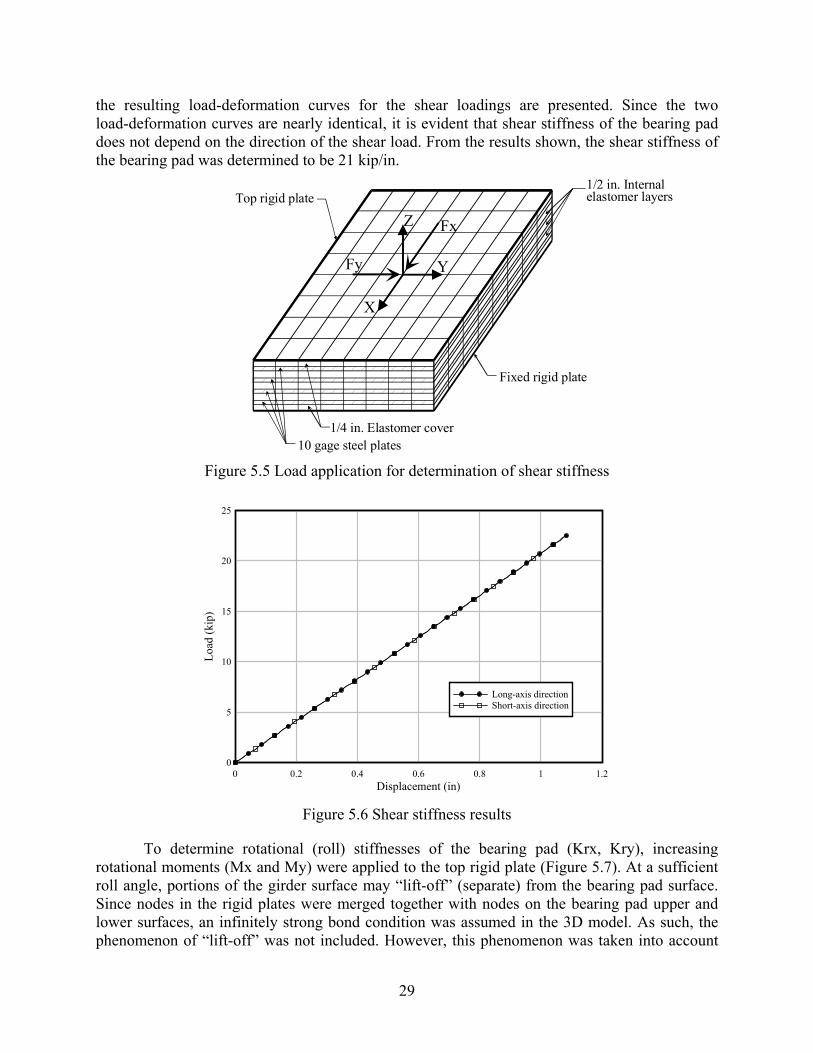
29
the resulting load-deformation curves for the shear loadings are presented. Since the two load-deformation curves are nearly identical, it is evident that shear stiffness of the bearing pad does not depend on the direction of the shear load. From the results shown, the shear stiffness of the bearing pad was determined to be 21 kip/in.
1/4 in. Elastomer cover10 gage steel plates
1/2 in. Internalelastomer layers
Fixed rigid plate
Top rigid plate
Z
X
Y
Fx
Fy
Figure 5.5 Load application for determination of shear stiffness
Displacement (in)
Load
(kip
)
0 0.2 0.4 0.6 0.8 1 1.20
5
10
15
20
25
Long-axis directionShort-axis direction
Figure 5.6 Shear stiffness results
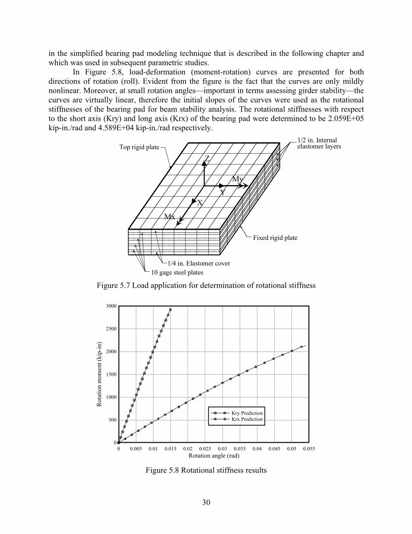
To determine rotational (roll) stiffnesses of the bearing pad (Krx, Kry), increasing rotational moments (Mx and My) were applied to the top rigid plate (Figure 5.7). At a sufficient roll angle, portions of the girder surface may “lift-off” (separate) from the bearing pad surface. Since nodes in the rigid plates were merged together with nodes on the bearing pad upper and lower surfaces, an infinitely strong bond condition was assumed in the 3D model. As such, the phenomenon of “lift-off” was not included. However, this phenomenon was taken into account
30
in the simplified bearing pad modeling technique that is described in the following chapter and which was used in subsequent parametric studies.
In Figure 5.8, load-deformation (moment-rotation) curves are presented for both directions of rotation (roll). Evident from the figure is the fact that the curves are only mildly nonlinear. Moreover, at small rotation angles—important in terms assessing girder stability—the curves are virtually linear, therefore the initial slopes of the curves were used as the rotational stiffnesses of the bearing pad for beam stability analysis. The rotational stiffnesses with respect to the short axis (Kry) and long axis (Krx) of the bearing pad were determined to be 2.059E+05 kip-in./rad and 4.589E+04 kip-in./rad respectively.
1/4 in. Elastomer cover10 gage steel plates
1/2 in. Internalelastomer layers
Fixed rigid plate
Top rigid plate
Z
XY
My
Mx
Figure 5.7 Load application for determination of rotational stiffness
Rotation angle (rad)
Rot
atio
n m
omen
t (ki
p-in
)
0 0.005 0.01 0.015 0.02 0.025 0.03 0.035 0.04 0.045 0.05 0.0550
500
1000
1500
2000
2500
3000
Kry PredictionKrx Prediction
Figure 5.8 Rotational stiffness results

31
In terms of assessing girder stability under skewed conditions, it is particularly important to quantify the rotation (roll) stiffness of the bearing pad at varying angles of skew. To consider skew effects, moments were applied to the bearing pad model at various angles of skew (Figure 5.9) and the resulting rotational responses computed. The moment-rotation curves obtained for the skew angles considered were essentially linear at small rotation angles, therefore the rotational stiffnesses were based on the initial stiffness data obtained. Rotational stiffnesses of the bearing pad for the skew angles analyzed here are presented in Figure 5.10.
1/4 in. Elastomer cover10 gage steel plates
1/2 in. Internalelastomer layers
Fixed rigid plate
Top rigid plate
Z
X
YMφ
φ
Figure 5.9 Load application for determination of skewed rotational stiffness
Skew angle (deg.)
Rot
atio
nal s
tiffn
ess (
kip-
in/ra
d)
0 10 20 30 40 50 60 70 80 9025000
50000
75000
100000
125000
150000
175000
200000
225000
Figure 5.10 Rotational stiffness vs. skew angle
Torsional pad stiffness was determined by applying a torsional moment to the top plate of the bearing pad model is shown in Figure 5.11. Since the shell elements use in the finite element
32
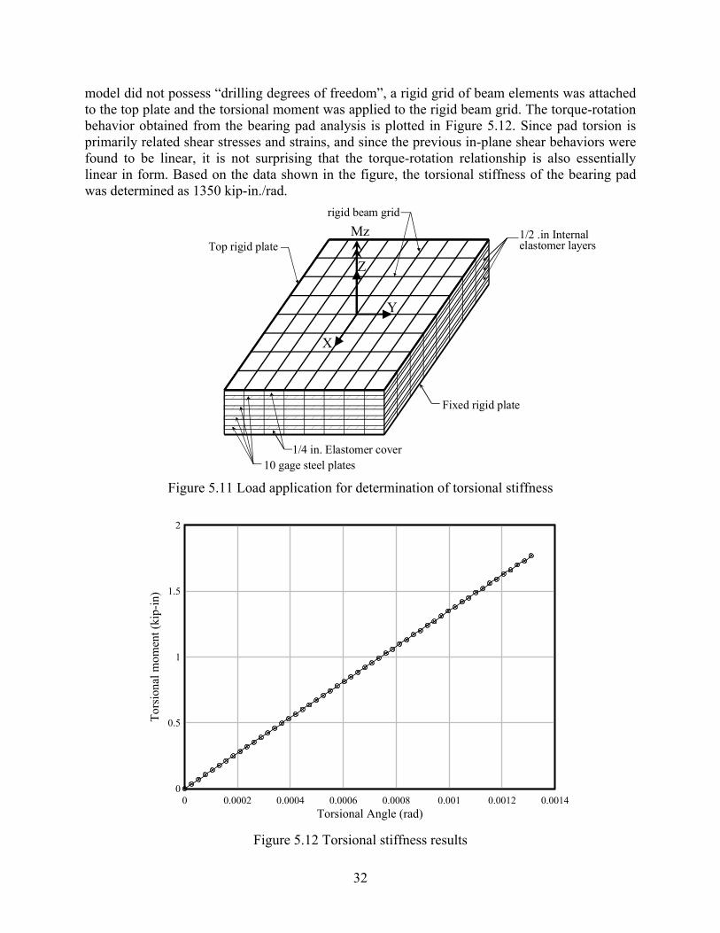
model did not possess “drilling degrees of freedom”, a rigid grid of beam elements was attached to the top plate and the torsional moment was applied to the rigid beam grid. The torque-rotation behavior obtained from the bearing pad analysis is plotted in Figure 5.12. Since pad torsion is primarily related shear stresses and strains, and since the previous in-plane shear behaviors were found to be linear, it is not surprising that the torque-rotation relationship is also essentially linear in form. Based on the data shown in the figure, the torsional stiffness of the bearing pad was determined as 1350 kip-in./rad.
1/4 in. Elastomer cover10 gage steel plates
1/2 .in Internal elastomer layers
Fixed rigid plate
Top rigid plate
Z
X
Y
Mzrigid beam grid
Figure 5.11 Load application for determination of torsional stiffness
Torsional Angle (rad)
Tors
iona
l mom
ent (
kip-
in)
0 0.0002 0.0004 0.0006 0.0008 0.001 0.0012 0.00140
0.5
1
1.5
2
Figure 5.12 Torsional stiffness results
33
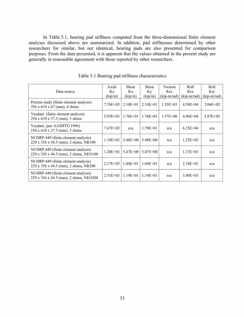
In Table 5.1, bearing pad stiffness computed from the three-dimensional finite element
analyses discussed above are summarized. In addition, pad stiffnesses determined by other researchers for similar, but not identical, bearing pads are also presented for comparison purposes. From the data presented, it is apparent that the values obtained in the present study are generally in reasonable agreement with those reported by other researchers.
Table 5.1 Bearing pad stiffness characteristics
Data source Axial
Kz (kip/in)
Shear Kx
(kip/in)
Shear Ky
(kip/in)
Torsion Krz
(kip-in/rad)
Roll Krx
(kip-in/rad)
Roll Kry
(kip-in/rad) Present study (finite element analysis) 356 x 610 x 67 (mm), 4 shims 7.76E+03 2.10E+01 2.10E+01 1.35E+03 4.59E+04 2.06E+05
Yazdani (finite element analysis) 254 x 610 x 37.5 (mm), 3 shims 5.95E+03 1.76E+01 1.76E+01 1.57E+00 4.96E+04 2.87E+05
Yazdani, (per AASHTO 1996) 254 x 610 x 37.5 (mm), 3 shims 7.47E+03 n/a 1.79E+01 n/a 6.23E+04 n/a
NCHRP-449 (finite element analysis) 229 x 356 x 44.5 (mm), 2 shims, NR100 1.18E+03 5.48E+00 5.48E+00 n/a 1.23E+03 n/a
NCHRP-449 (finite element analysis) 229 x 356 x 44.5 (mm), 2 shims, NEO100 1.20E+03 5.47E+00 5.47E+00 n/a 1.37E+03 n/a
NCHRP-449 (finite element analysis) 229 x 356 x 44.5 (mm), 2 shims, NR200 2.17E+03 1.04E+01 1.04E+01 n/a 2.34E+03 n/a
NCHRP-449 (finite element analysis) 229 x 356 x 44.5 (mm), 2 shims, NEO200 2.51E+03 1.19E+01 1.19E+01 n/a 3.49E+03 n/a
34
CHAPTER 6 SIMPLIFIED BEARING MODEL
6.1 Introduction
Three-dimensional solid modeling and analysis, of the type described in the previous chapter, is generally the most accurate computational means available for analyzing bearing pad behavior. However, combining such models together with girder and bracing elements for the purpose of analyzing girder stability yields a computationally demanding analysis situation. If such analyses are to be performed thousands of times as part of an overall parametric study, the computational demands of this approach become problematic. Therefore, a simplified bearing pad model was devised using data obtained from the previously discussed three-dimensional analyses. The simplified bearing pad models were created by using a combination of rigid-beam grids, spring elements, gap (zero-tension) elements, and truss elements to simulate pad behavior (including creep) and interaction between a pad and the girder (lift-off behavior).
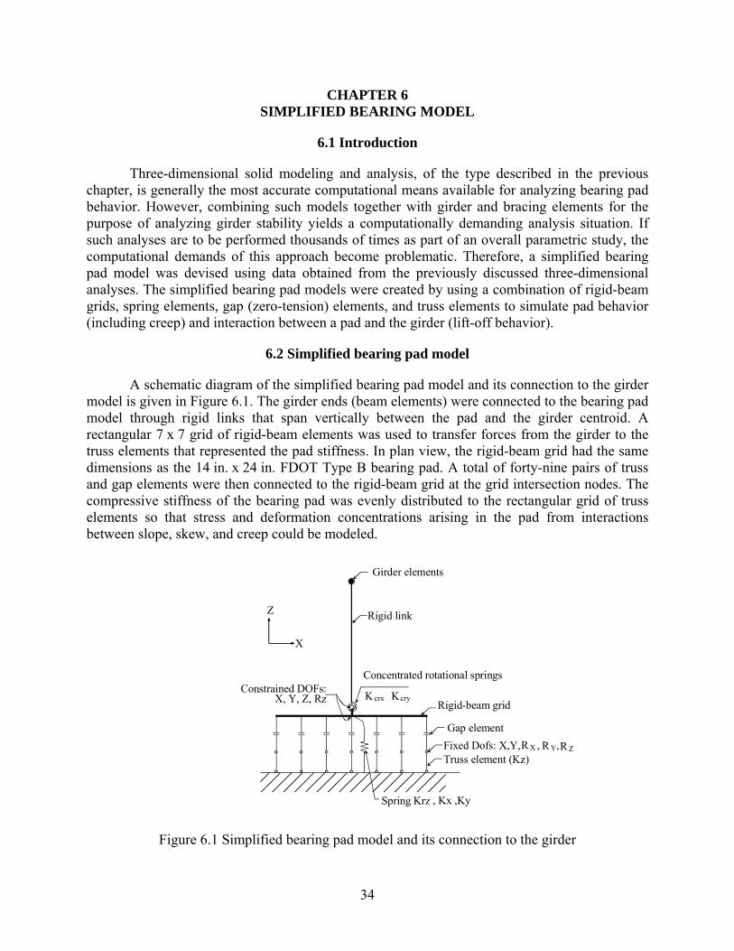
6.2 Simplified bearing pad model
A schematic diagram of the simplified bearing pad model and its connection to the girder model is given in Figure 6.1. The girder ends (beam elements) were connected to the bearing pad model through rigid links that span vertically between the pad and the girder centroid. A rectangular 7 x 7 grid of rigid-beam elements was used to transfer forces from the girder to the truss elements that represented the pad stiffness. In plan view, the rigid-beam grid had the same dimensions as the 14 in. x 24 in. FDOT Type B bearing pad. A total of forty-nine pairs of truss and gap elements were then connected to the rigid-beam grid at the grid intersection nodes. The compressive stiffness of the bearing pad was evenly distributed to the rectangular grid of truss elements so that stress and deformation concentrations arising in the pad from interactions between slope, skew, and creep could be modeled.
Girder elements
Rigid link
Rigid-beam gridK crx
Concentrated rotational springs
Kcry
Gap elementFixed Dofs: X,Y, , , R X R Y R ZTruss element (Kz)
Spring Krz , Kx ,Ky
Constrained DOFs:X, Y, Z, Rz
Z
X
Figure 6.1 Simplified bearing pad model and its connection to the girder
35
However, it must be noted that even under concentric loading conditions without skew or slope, the vertical pressure distribution in a bearing pad is non-uniform in nature with maximum pressure occurring at the center (due to confinement) and minimum pressures occurring along the edges. As a result, a simplified bearing pad model employing evenly-distributed stiffness (truss elements) will generally over-predict the rotational stiffnesses of the pad. As will be discussed later, appropriate rotational pad stiffnesses were achieved in this study by combining additional concentrated rotational springs in series with the grid of equal-stiffness truss elements. Series combination of concentrated rotational springs with the grid of truss elements had the effect of softening the overall rotational stiffness of the simplified pad model.
To enable the simplified model to account for the effects of creep, a power creep law of the form:
a a1 2c 0ε (t) = a σ t (6.1)
was introduced into each truss element in the bearing pad grid. In the equation above, 0a , 1a , and 2a are material constants that control the rate of creep as functions of stress and time. The specific values of 0a , 1a , and 2a were presented earlier in this report.
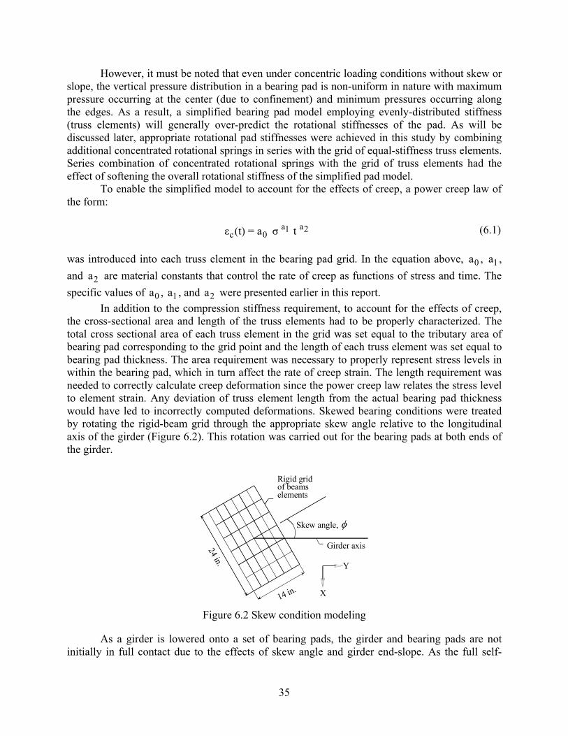
In addition to the compression stiffness requirement, to account for the effects of creep, the cross-sectional area and length of the truss elements had to be properly characterized. The total cross sectional area of each truss element in the grid was set equal to the tributary area of bearing pad corresponding to the grid point and the length of each truss element was set equal to bearing pad thickness. The area requirement was necessary to properly represent stress levels in within the bearing pad, which in turn affect the rate of creep strain. The length requirement was needed to correctly calculate creep deformation since the power creep law relates the stress level to element strain. Any deviation of truss element length from the actual bearing pad thickness would have led to incorrectly computed deformations. Skewed bearing conditions were treated by rotating the rigid-beam grid through the appropriate skew angle relative to the longitudinal axis of the girder (Figure 6.2). This rotation was carried out for the bearing pads at both ends of the girder.
24 in.
14 in.
Rigid gridof beamselements
Girder axis
Skew angle,
X
Y
φ
Figure 6.2 Skew condition modeling
As a girder is lowered onto a set of bearing pads, the girder and bearing pads are not initially in full contact due to the effects of skew angle and girder end-slope. As the full self-
36
weight of the girder is released from the lifting cables and applied to the bearing pads, the distribution of stresses and deformations within the pads will not be uniform. Rather, very high stresses will be present in areas where initial contact is made. The final distribution of stresses in the pad depends on the pad stiffness and on the nature of the initial gap that exists between the bearing pad and the sloped girder ends. In the simplified bearing pad model, this behavior was modeled by attaching each truss element in the pad grid to a “gap element”. Gap elements are spring elements that have zero tension stiffness and zero compression stiffness until a specified compressive activation deformation level is reached. Once the activation deformation has been reached—i.e., the gap has “closed”—the stiffness of the spring takes on the specified compressive stiffness. This behavior is illustrated in Figure 6.3. Since the correct compressive stiffness of the bearing pad was already incorporated into the truss elements, it was necessary to give the gap elements nearly infinite compressive stiffness so that their presence did not alter the overall stiffness of truss-gap combination. This was achieved by specifying gap element compressive stiffnesses that were very large relative the bearing pad truss element stiffnesses, but not so large as to ill-condition the stiffness matrix of the entire system.
Compressive gap
Force(tension)
Deformation(tension)
kgap
Deformation(compression)
Force(compression)
kgap >> k truss
Compressiveactivationdeformationlevel
( )
Zero stiffnessin tension
Figure 6.3 Force-deformation curve for a gap element
By employing a zero tension stiffness, the use of gap elements also permits modeling of girder lift-off from the pad. Lift-off occurs when loading on the girder causes the girder to physically lift-off (separate) from a portion of the bearing pads. Such conditions may arise at the point of buckling instability under vertical loading and at the point of rollover under lateral wind loading. By using zero tension stiffness gap elements, the simplified model is capable of correctly representing occurrences of lift-off.
For each gap element in the pad grid, the gap size (activation deformation) had to be specified. At the location where initial contact is made between the girder and pad, the gap size was specified as zero. For conditions of combined skew and girder end-slope, initial contact occurs at a single grid point located at one corner of the pad. In an unskewed condition with girder end-slope, initial contact occurs along a line of grid points that span the width of the pad. For gap elements not located at the point of initial contact, the magnitude of activation deformation was calculated as the physical size of the vertical gap between the pad and the girder. In Figure 6.4 gap element activation deformations are illustrated for a system with end-rotation but without skew.
37
Slopeangle
Bearing pad
Girder
Rigid link
Slopeangle
Truss elements
Gap elements (not shown to scale)
Slopeangle
Girder centroid
Location of initial contact
Activation deformation iszero at point ofinitial contact
Rigid grid of beam elements
Bearing padthickness
Activation deformationsfor gap elements not atinitial point of contact
Girder
Concentrated rotational springs (Kcrx, Kcry)
Concentrated springs (Krz, Kx,Ky)
Figure 6.4 Gap element activation deformations for end-slope case
When the vertical stiffnesses of all truss elements in the simplified bearing pad model were summed together, their total compressive stiffness matched that computed from compressive loading of the detailed three-dimensional (solid element) bearing pad models discussed in the previous chapter. However, when moment loads were applied to the simplified bearing pad model, the rotational stiffnesses obtained were generally larger then the results previously obtained from detailed three-dimensional analyses. This is due to the fact that a grid of discrete truss elements cannot completely capture the three-dimensional stress states that arise in the actual layered bearing pad. In order to correct this problem and ensure that the simplified model yielded not only the correct compressive stiffness but also the correct rotational stiffnesses, additional concentrated rotational spring elements—connecting the rigid links to the rigid grid (Figure 6.4)—were combined with the grid of discrete truss and gap elements. For each axis of rotation, the concentrated springs were combined in series with the summed effect of the discrete truss elements. Stiffness values for the concentrated rotational springs were computed such that the effective series stiffness of the combination of concentrated spring and truss grid produced the desired rotational stiffness (as obtained from earlier three-dimensional analysis). The concentrated rotational spring stiffnesses for the x- and y-axes (Figure 6.2) were computed as follows:
3D(90- ) trussr rx
crx truss 3D(90- )rx r
k kK = k - k
φ
φ (6.2)
3D( ) trussr ry
cry truss 3D( )ry r
k kK =
k - k
φ
φ (6.3)
In the equations above, φ is the skew angle of the girder, 3D( )rk φ and 3D(90- )
rk φ are the rotational stiffnesses obtained from detailed three-dimensional (3D) analyses for skew angles of φ and
38
(90 )φ− respectively, and trussrxk and truss
ryk are the rotational stiffnesses contributed by the grid of truss elements about the x- and y-axes respectively.
In addition to representing the compressive axial stiffness (Kz) and rotational stiffnesses (Krx, Kry) of the pad, the simplified model also had to represent the torsional stiffness (Krz) and shear stiffnesses (Kx and Ky in the x- and y-directions) of the pad. Modeling the latter stiffnesses required only that springs (Krz, Kx, Ky) be connected from the rigid grid to the support (Figure 6.4). The values of Krz, Kx, and Ky used in the simplified model were those obtained directly from the detailed three-dimensional analyses discussed in the previous chapter.
Connection of the vertical link to the simplified bearing pad model involved use of the concentrated rotational springs (Kcrx, and Kcry) and additional degree of freedom (DOF) constraints. Specifically, the x-, y-, and z-direction translational DOFs and the z-direction rotational DOF at the bottom of the vertical link were constrained to match the DOFs (displacements and rotation) at the center node of the rigid grid (Figure 6.5).
Master nodeSlave node
Constrained degrees offreedom: X, Y, Z, Rz
Rigid grid ofbeam elements
Rigid link
Girder centroid
Truss elements
Gap elements (not shown to scale)
Concentrated rotational springs (Kcrx, Kcry)
Figure 6.5 Connection of vertical link to rigid grid
39
CHAPTER 7 BUCKLING ANALYSIS PROCEDURES
7.1 Introduction
The most common approach to numerically computing buckling loads is to solve a linearized eigenvalue/eigenvector buckling problem. Most general-purpose finite element analysis software packages, including ADINA, offer the ability to solve for buckling loads using this approach. However, there are limitations to this method. Time-dependent effects such as creep, geometric nonlinearity, and material nonlinearity can only be approximately incorporated into the linearized eigen problem.
An alternative to this approach involves the use of large displacement analysis. In this approach, loads are incrementally applied to the structure, and at each level of loading, static equilibrium of the structure (stability) is solved for in the deformed configuration of the structure (i.e., taking into account the changes of geometry that have occurred as a result of the loads). In order to use such an approach to solve buckling problems, member imperfections (e.g., sweep) must be introduced into the initial configuration of the structure. There are several advantages to this approach. Because imperfections are included as part of the analysis, the sensitivity of buckling loads (system stability) to the magnitude of such imperfections, can be quantified directly. Also, because loads are incrementally applied, a physical time scale can be attached to the analysis so that time-dependent effects, such as creep, can be included. Finally, material non-linerarities associated with the use of gap elements can also be directly taken into account using this approach. For these reasons, large displacement analysis of systems with initial imperfections was the primary approach used throughout this study when conducting system stability analyses.
7.2 Girder-buckling system model
Numerical determination of buckling loads were carried out by conducting large displacement analyses on system-level models that combined girder elements, simplified bearing pad models, and—in most cases—lateral bracing at the girder ends. Conceptual sketches of the finite element model of a girder on bearing pads with geometric sweep, skew, and slope are shown in Figure 7.1. For computational efficiency, resultant beam elements were used to model the girder. Resultant beam elements are elements in which the resultant cross-sectional properties (area, moments of inertia, torsional constant) are specified rather than the specific cross-sectional geometry (dimensions) being specified. The girder elements were geometrically located at the center of gravity (C.G.) of the girder. A linear elastic material model was used for the concrete girder with an elastic (Young’s) modulus of 4930 ksi and Poisson’s ratio of ν = 0.20. Sweep imperfection of the girder was introduced by superimposing a sinusoidal shape on the girder in the lateral direction with maximum sweep occurring at mid-span. Inclusion of sweep in the girder model not only represented the actual manufactured condition of the girder, but also initiated triggering of girder instability under the applied loads.
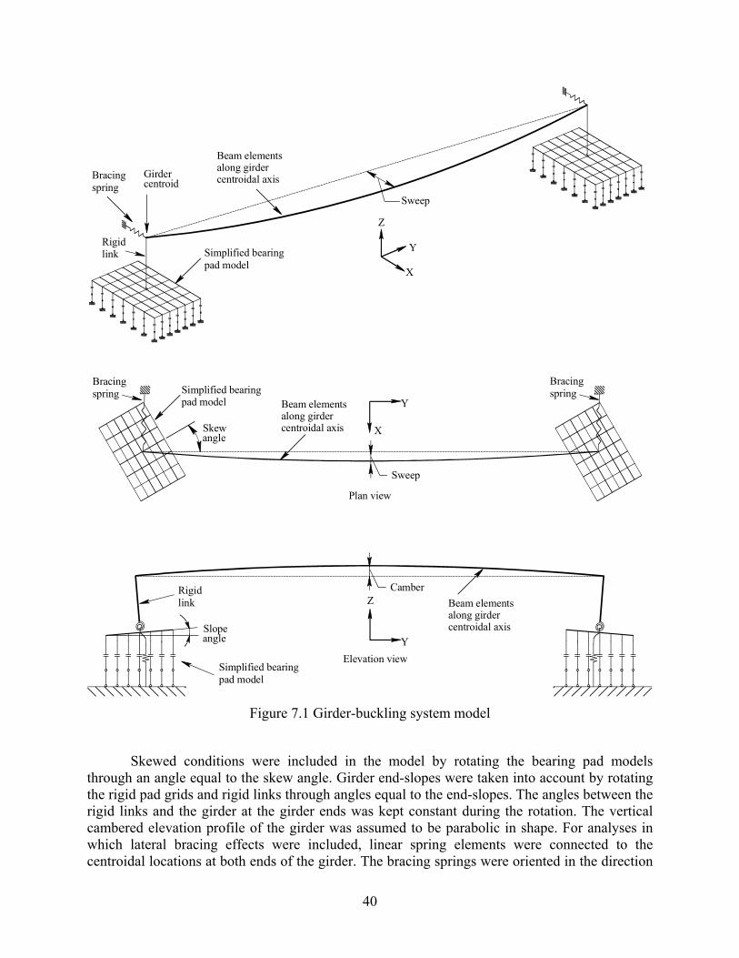
40
Sweep
X
Y
Z
X
Y
Sweep
Simplified bearingpad model
Bracingspring
Girder centroid
Simplified bearingpad model
Skewangle
Beam elementsalong girder centroidal axis
Camber
Slopeangle
Beam elementsalong girder centroidal axis
Beam elementsalong girder centroidal axis
Simplified bearingpad model
Y
Z
Plan view
Elevation view
Rigidlink
Rigidlink
Bracingspring
Bracingspring
Figure 7.1 Girder-buckling system model
Skewed conditions were included in the model by rotating the bearing pad models through an angle equal to the skew angle. Girder end-slopes were taken into account by rotating the rigid pad grids and rigid links through angles equal to the end-slopes. The angles between the rigid links and the girder at the girder ends was kept constant during the rotation. The vertical cambered elevation profile of the girder was assumed to be parabolic in shape. For analyses in which lateral bracing effects were included, linear spring elements were connected to the centroidal locations at both ends of the girder. The bracing springs were oriented in the direction

41
of lateral girder displacement. Thus, bracing stiffnesses considered in this study were effective at the centroidal elevation of the girder and in the direction perpendicular to the longitudinal axis of the girder.
7.3 Loading procedure used for buckling analysis
Loads applied to the girder for the purpose of determining buckling capacities were distributed uniformly along girder length (Figure 7.2). For analyses in which creep effects were excluded, the loading procedure (Figure 7.3) consisted of two stages: 1) ramping the load to the self-weight of the girder and, 2) ramping the load until girder instability occurred. When creep effects were included, the loading procedure (Figure 7.4) consisted of three stages: 1) ramping the load to the self-weight of the girder, 2) maintaining self-weight load on the girder (and pads) for 72 hours, and 3) ramping the load until girder instability occurred. In all cases, prior to application of any load, ten (10) stabilizing linear springs were provided at each end of the girder. These stabilizing springs were particularly necessary for analyses of unbraced-girders in which the combined effects of skew and slope were included. For such cases, initial contact between the girder and pad was isolated to a single grid point in the pad model. As a result, the bearing pad initially provides no rotational stiffnesses to restrain the girder from rigid-body rotation and subsequent rollover.
Sweep
X
Y
Z
Uniform load
Beam elementsalong girder centroidal axis
Simplified bearingpad model
Bracingspring
Ten stabilization braces (springs)
Rigidlink
Figure 7.2 Load application on girder-buckling system
In reality however, between the point of initial contact and the point at which the full self-weight of the girder rests on the bearing pads, the girder is supported and stabilized by the upward forces of the lifting cables. The stabilizing effect of the lifting cable forces is at its maximum when the girder initially comes into contact with the pads and vanishes at the point where the cables go slack and the full self-weight of the beam rests on the pads. The numeric approach used to approximately simulate this effect was to add ten stabilization braces to each end of the girder. At time zero, all ten braces at each girder end are active. As the loading on the girder is ramped up from zero to the full girder self-weight, the stabilization braces are gradually

42
removed—one brace at each end is removed for every 1/10th of the girder self-weight load that is applied (Figure 7.3). In this manner, when the full self-weight load is reached, all stabilization braces have been removed. If the analysis being performed is an unbraced analysis, then no braces will be present as load is ramped up beyond the self-weight load. If a braced case is being analyzed, then only the bracing stiffness under consideration will be present for loads that exceed the girder self-weight.
w selfweight
w critical
Applied uniform load
Time
Number of stabilization springs active at each end of girder model
Load at whichgirder instability(buckling) occurs
10 9 8 7 6 5 4 3 2 1 0 0
30 sec. self-weight loading
Figure 7.3 Load procedure used for buckling analysis with creep effects excluded
w selfweight
w critical
Applied uniform load
Time
Number of stabilization springs active at each end of girder model
Load at whichgirder instability(buckling) occurs
10
72 hr. self-weight creep
9 8 7 6 5 4 3 2 1 0 0
30 sec. self-weight loading
Figure 7.4 Load procedure used for buckling analysis with creep effects included
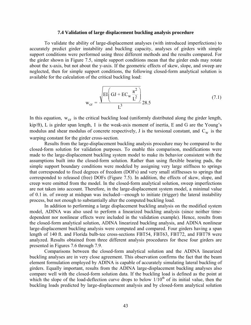
43
7.4 Validation of large displacement buckling analysis procedure
To validate the ability of large-displacement analyses (with introduced imperfections) to accurately predict girder instability and buckling capacity, analyses of girders with simple support conditions were performed using three different methods and the results compared. For the girder shown in Figure 7.5, simple support conditions mean that the girder ends may rotate about the x-axis, but not about the y-axis. If the geometric effects of skew, slope, and sweep are neglected, then for simple support conditions, the following closed-form analytical solution is available for the calculation of the critical buckling load:
2
w 2
cr 3
πEI GJ + ECL
w = 28.5L
⎛ ⎞⎜ ⎟⎜ ⎟⎝ ⎠
(7.1)
In this equation, crw is the critical buckling load (uniformly distributed along the girder length, kip/ft), L is girder span length, I is the weak-axis moment of inertia, E and G are the Young’s modulus and shear modulus of concrete respectively, J is the torsional constant, and wC is the warping constant for the girder cross-section.
Results from the large-displacement buckling analysis procedure may be compared to the closed-form solution for validation purposes. To enable this comparison, modifications were made to the large-displacement buckling system model to make its behavior consistent with the assumptions built into the closed-form solution. Rather than using flexible bearing pads, the simple support boundary conditions were modeled by assigning very large stiffness to springs that corresponded to fixed degrees of freedom (DOFs) and very small stiffnesses to springs that corresponded to released (free) DOFs (Figure 7.5). In addition, the effects of skew, slope, and creep were omitted from the model. In the closed-form analytical solution, sweep imperfections are not taken into account. Therefore, in the large-displacement system model, a minimal value of 0.1 in. of sweep at midspan was included—enough to initiate (trigger) the lateral instability process, but not enough to substantially alter the computed buckling load.
In addition to performing a large displacement buckling analysis on the modified system model, ADINA was also used to perform a linearized buckling analysis (since neither time-dependent nor nonlinear effects were included in the validation example). Hence, results from the closed-form analytical solution, ADINA linearized buckling analysis, and ADINA nonlinear large-displacement buckling analysis were computed and compared. Four girders having a span length of 140 ft. and Florida bulb-tee cross-sections FBT54, FBT63, FBT72, and FBT78 were analyzed. Results obtained from three different analysis procedures for these four girders are presented in Figures 7.6 through 7.9.
Comparisons between the closed-form analytical solution and the ADINA linearized buckling analyses are in very close agreement. This observation confirms the fact that the beam element formulation employed by ADINA is capable of accurately simulating lateral buckling of girders. Equally important, results from the ADINA large-displacement buckling analyses also compare well with the closed-form solution data. If the buckling load is defined as the point at which the slope of the load-deflection curve drops to below 1/10th of its initial value, then the buckling loads predicted by large-displacement analysis and by closed-form analytical solution
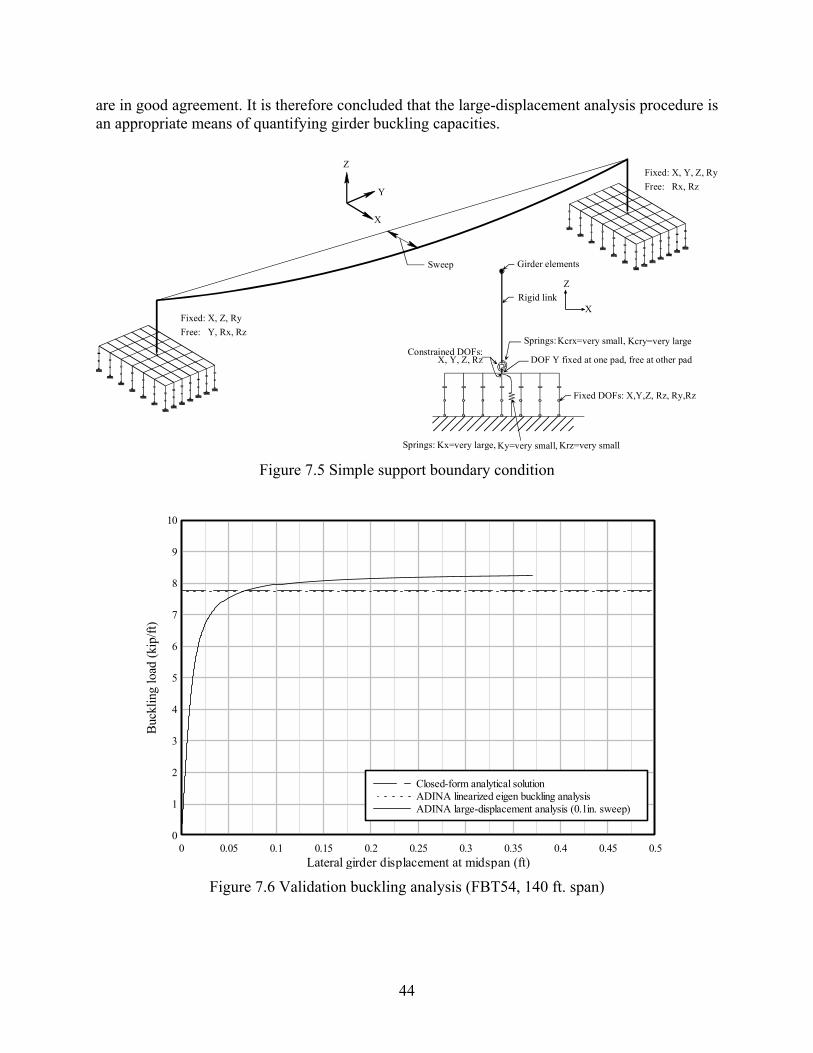
44
are in good agreement. It is therefore concluded that the large-displacement analysis procedure is an appropriate means of quantifying girder buckling capacities.
Girder elements
Rigid link
Springs:
Constrained DOFs:X, Y, Z, Rz
Z
X
Springs:
Sweep
Fixed: X, Z, RyFree: Y, Rx, Rz
Fixed: X, Y, Z, RyFree: Rx, Rz
X
Y
Z
Kcrx=very small,
Kx=very large, Ky=very small , Krz=very small
Kcry=very large
Fixed DOFs: X,Y,Z, Rz, Ry,Rz
DOF Y fixed at one pad, free at other pad
Figure 7.5 Simple support boundary condition
Lateral girder displacement at midspan (ft)
Buck
ling
load
(kip
/ft)
0 0.05 0.1 0.15 0.2 0.25 0.3 0.35 0.4 0.45 0.50
1
2
3
4
5
6
7
8
9
10
Closed-form analytical solutionADINA linearized eigen buckling analysisADINA large-displacement analysis (0.1in. sweep)
Figure 7.6 Validation buckling analysis (FBT54, 140 ft. span)
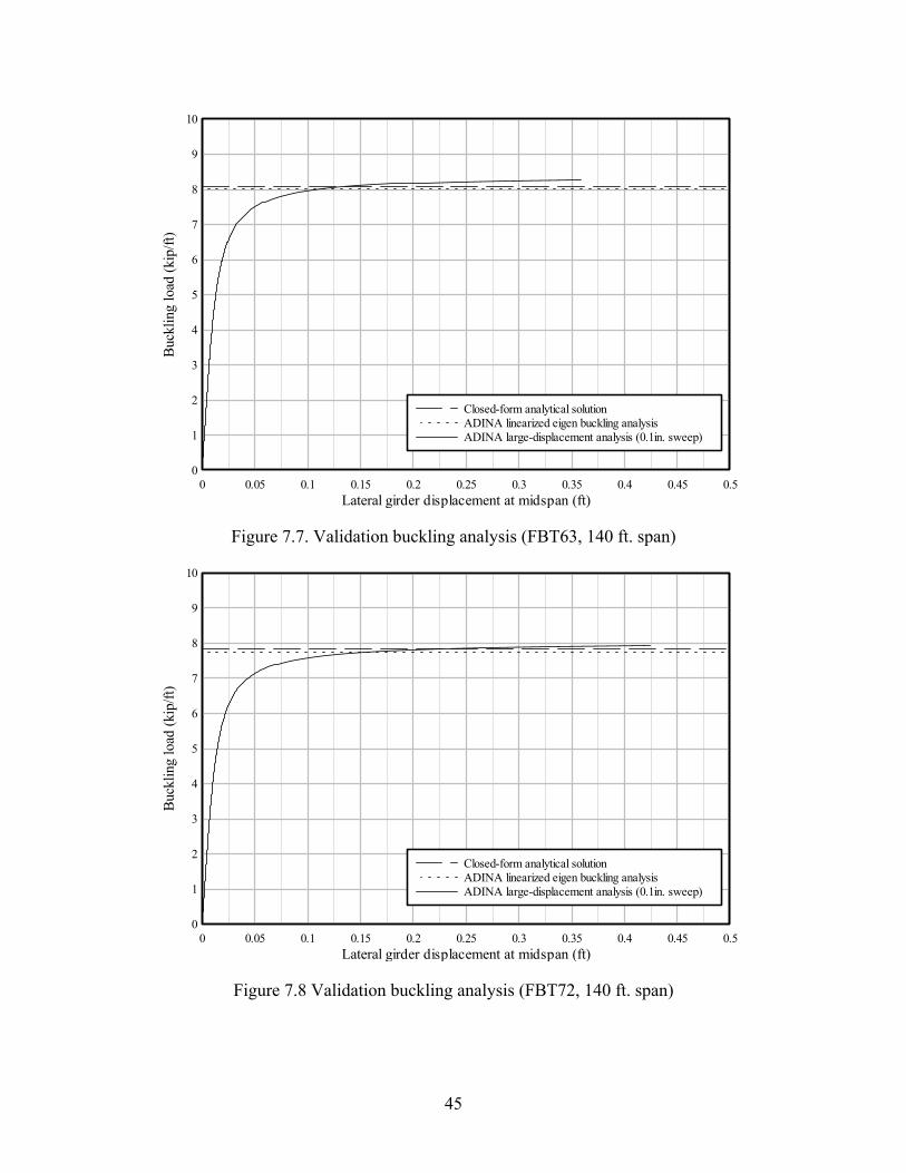
45
Lateral girder displacement at midspan (ft)
Buck
ling
load
(kip
/ft)
0 0.05 0.1 0.15 0.2 0.25 0.3 0.35 0.4 0.45 0.50
1
2
3
4
5
6
7
8
9
10
Closed-form analytical solutionADINA linearized eigen buckling analysisADINA large-displacement analysis (0.1in. sweep)
Figure 7.7. Validation buckling analysis (FBT63, 140 ft. span)
Lateral girder displacement at midspan (ft)
Buck
ling
load
(kip
/ft)
0 0.05 0.1 0.15 0.2 0.25 0.3 0.35 0.4 0.45 0.50
1
2
3
4
5
6
7
8
9
10
Closed-form analytical solutionADINA linearized eigen buckling analysisADINA large-displacement analysis (0.1in. sweep)
Figure 7.8 Validation buckling analysis (FBT72, 140 ft. span)
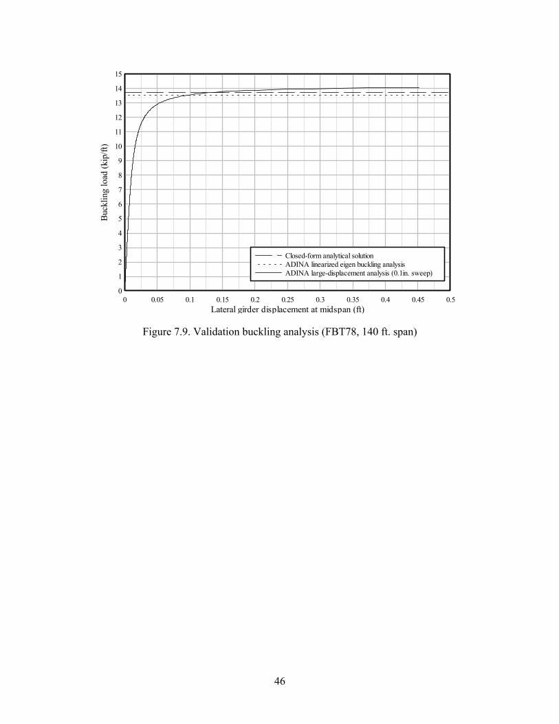
46
Lateral girder displacement at midspan (ft)
Buck
ling
load
(kip
/ft)
0 0.05 0.1 0.15 0.2 0.25 0.3 0.35 0.4 0.45 0.50
1
2
3
4
5
6
7
8
9
10
11
12
13
14
15
Closed-form analytical solutionADINA linearized eigen buckling analysisADINA large-displacement analysis (0.1in. sweep)
Figure 7.9. Validation buckling analysis (FBT78, 140 ft. span)

47
CHAPTER 8 BUCKLING ANALYSIS RESULTS
8.1 Introduction
Using the girder, simplified bearing pad, and bracing models described in previous chapters, a comprehensive parametric study was carried out using numerical simulation to quantify girder buckling capacities over a variety of different potential field conditions. System parameters that most strongly influenced girder buckling capacity were identified through sensitivity studies. Subsequently, simplified equations were developed for conservatively estimating girder buckling capacity under varied field conditions.
8.2 Parameter descriptions
The characteristic system parameters that were varied in the parametric study were as follows:
• Girder type (cross-sectional properties) • Span length • Skew angle • Bearing slope angle • Lateral sweep • Bearing pad creep (included or neglected) • Bracing stiffness
For each buckling analysis conducted, a single set of values were selected from those listed in Table 8.1. In total, 4800 different buckling analyses were performed. For each of the four Florida bulb-tee (FBT) girder types considered, a series of four different span lengths were analyzed. It is important to note that the maximum span length considered for each girder may not represent feasible situations from a design perspective even though stability analyses could be performed (this issue will be discussed in more detail later in this chapter). The maximum span lengths considered in this study were included primarily to ensure that abrupt changes in data trends did not occur just beyond the practical ranges of interest.
Table 8.1 Values used in parametric study
Girder type: Span length: FBT54 80 ft 100 ft 120 ft 140 ft FBT63 100 ft 120 ft 140 ft 160 ft FBT72 120 ft 140 ft 160 ft 180 ft FBT78 140 ft 160 ft 180 ft 200 ft
Skew angle: Slope angle: Girder sweep Bearing pad creep Bracing stiffness:
0 deg. 0.00 rad. 0.5 in. Included 0 kip/in 15 deg. 0.05 rad. 1.5 in. Neglected 10 kip/in 30 deg. 2.5 in. 100 kip/in 45 deg. 1000 kip/in 60 deg. 10,000 kip/in

48
Multiple skew angles ranging from 0 deg. (unskewed) to 60 deg. were used to quantify the effects of skew girder stability. Similar to the comment noted above regarding maximum selected span lengths, the maximum considered skew angle of 60 deg. was included to extend the range of numerical evaluation beyond the practical range of interest.
Selection of the maximum considered slope angle was based on examining the combined effects of camber (due to girder prestressing), roadway grade, and construction tolerance. Based on a review of pertinent design calculations for long-span prestressed concrete girders, an end slope (rotation) of 1 deg. (0.0175 rad.) was determined to be a reasonable upper limit on camber induced slope. In regard to roadway grade, the FDOT bridge design standards (2006 Index No. 20500) require that beveled bearing plates be used whenever the beam grade exceeds a slope of 2% (0.0200 rad.). As such, this angle was considered to be the maximum possible grade-related slope mismatch that would occur between the girder and the bearing pad. Finally, the AASHTO LRFD Bridge Design Specifications (AASHTO 2004) stipulate that allowance for a rotation angle of 0.0050 rad. be considered to account for construction related tolerances. Summing these slopes gives 0.0175 + 0.0200 + 0.0050 = 0.0425 which was conservatively rounded up to 0.05 rad. and then selected as the maximum slope angle to be used in the parametric study.
The maximum girder sweep imperfection value was established based on a review of several bridge design documents as well as discussions with FDOT engineers. In the 1991 FDOT Standard Specifications for Road and Bridge Construction (FDOT 1991), maximum allowable girder sweep was limited to 1/8 in. of sweep per 10 ft of girder length, but not to exceed 1.5 in. In the 2004 FDOT standard specifications, maximum sweep was limited to 1/8 in. per 10 ft of length, but with no upper bound. Most recently, in the 2006 FDOT standard specifications, maximum permissible sweep was once again 1/8 in. per 10 ft of length, but with a maximum upper limit of 1.5 in. In PCI Manual 116-99: Quality Control for Plants and Production of Structural Precast Concrete Products, (PCI 1999), maximum permissible sweep is specified as 1/8 in. per 10 ft of length, but with no upper limit.
At the 80 ft minimum span length considered in this study (Table 8.1), the 1/8 in. per 10 ft criterion yields a maximum allowable sweep of 1.0 in. When applied to the 200 ft maximum span length considered, the same criterion yields a sweep of 2.5 in. However, the latter value exceeds the current FDOT upper limit of 1.5 in., therefore 1.5 in would control instead. According to the current FDOT standards then, the maximum sweep values applicable to the span lengths considered here would range from 1.0 to 1.5 in. Slightly wider ranging values—0.5 in., 1.5 in., and 2.5 in.—were instead selected for this study so that an adequate spread would be available for the purpose of evaluating the sensitivity of buckling capacity to sweep imperfection. All of the sweep values considered here were, however, conservative in comparison to currently applicable FDOT standards.
As indicated in Table 8.1, moderate term (72 hr) creep effects in the bearing pads were either included (taken into account) or excluded (neglected). However, no further refinements to the creep characteristics of the bearings were included. The power law creep parameters used in the “creep-included” simulations were presented earlier in this report.
Bracing stiffnesses ranged from zero (an unbraced condition) to 10,000 kip/in. It must be clearly noted that the bracing stiffnesses used in this study were stiffnesses effective at the centroid of the girder and for a bracing direction that was perpendicular to the longitudinal axis (direction of span) of the girder. Due to the increased moment-arm, bracing elements attached to the top flange or upper sections of the girder would be more effective than bracing connected at
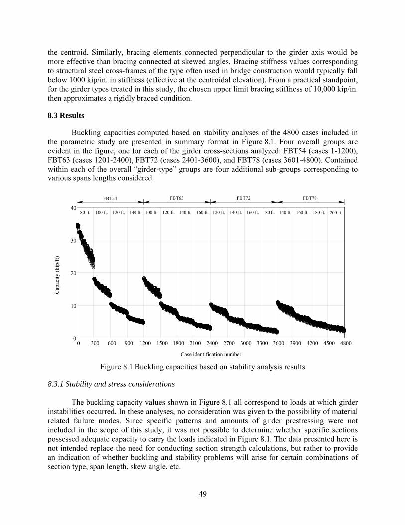
49
the centroid. Similarly, bracing elements connected perpendicular to the girder axis would be more effective than bracing connected at skewed angles. Bracing stiffness values corresponding to structural steel cross-frames of the type often used in bridge construction would typically fall below 1000 kip/in. in stiffness (effective at the centroidal elevation). From a practical standpoint, for the girder types treated in this study, the chosen upper limit bracing stiffness of 10,000 kip/in. then approximates a rigidly braced condition.
8.3 Results
Buckling capacities computed based on stability analyses of the 4800 cases included in the parametric study are presented in summary format in Figure 8.1. Four overall groups are evident in the figure, one for each of the girder cross-sections analyzed: FBT54 (cases 1-1200), FBT63 (cases 1201-2400), FBT72 (cases 2401-3600), and FBT78 (cases 3601-4800). Contained within each of the overall “girder-type” groups are four additional sub-groups corresponding to various spans lengths considered.
0 300 600 900 1200 1500 1800 2100 2400 2700 3000 3300 3600 3900 4200 4500 48000
10
20
30
40
Case identification number
Cap
acity
(kip
/ft)
FBT54 FBT63 FBT72 FBT78
80 ft. 100 ft. 120 ft. 140 ft. 100 ft. 120 ft. 140 ft. 160 ft. 120 ft. 140 ft. 160 ft. 180 ft. 140 ft. 160 ft. 180 ft. 200 ft.
Figure 8.1 Buckling capacities based on stability analysis results
8.3.1 Stability and stress considerations
The buckling capacity values shown in Figure 8.1 all correspond to loads at which girder instabilities occurred. In these analyses, no consideration was given to the possibility of material related failure modes. Since specific patterns and amounts of girder prestressing were not included in the scope of this study, it was not possible to determine whether specific sections possessed adequate capacity to carry the loads indicated in Figure 8.1. The data presented here is not intended replace the need for conducting section strength calculations, but rather to provide an indication of whether buckling and stability problems will arise for certain combinations of section type, span length, skew angle, etc.
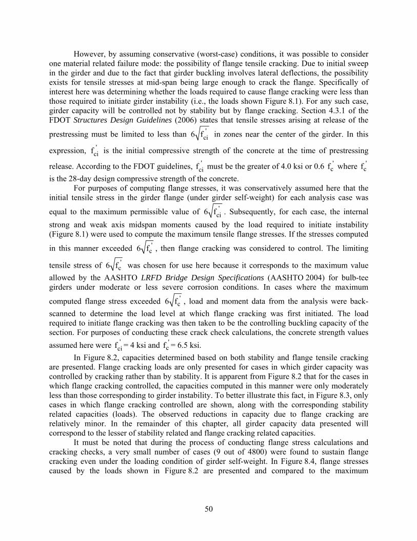
50
However, by assuming conservative (worst-case) conditions, it was possible to consider one material related failure mode: the possibility of flange tensile cracking. Due to initial sweep in the girder and due to the fact that girder buckling involves lateral deflections, the possibility exists for tensile stresses at mid-span being large enough to crack the flange. Specifically of interest here was determining whether the loads required to cause flange cracking were less than those required to initiate girder instability (i.e., the loads shown Figure 8.1). For any such case, girder capacity will be controlled not by stability but by flange cracking. Section 4.3.1 of the FDOT Structures Design Guidelines (2006) states that tensile stresses arising at release of the
prestressing must be limited to less than 'ci6 f in zones near the center of the girder. In this
expression, 'cif is the initial compressive strength of the concrete at the time of prestressing
release. According to the FDOT guidelines, 'cif must be the greater of 4.0 ksi or 0.6 '
cf where 'cf
is the 28-day design compressive strength of the concrete. For purposes of computing flange stresses, it was conservatively assumed here that the
initial tensile stress in the girder flange (under girder self-weight) for each analysis case was
equal to the maximum permissible value of 'ci6 f . Subsequently, for each case, the internal
strong and weak axis midspan moments caused by the load required to initiate instability (Figure 8.1) were used to compute the maximum tensile flange stresses. If the stresses computed
in this manner exceeded 'c6 f , then flange cracking was considered to control. The limiting
tensile stress of 'c6 f was chosen for use here because it corresponds to the maximum value
allowed by the AASHTO LRFD Bridge Design Specifications (AASHTO 2004) for bulb-tee girders under moderate or less severe corrosion conditions. In cases where the maximum
computed flange stress exceeded 'c6 f , load and moment data from the analysis were back-
scanned to determine the load level at which flange cracking was first initiated. The load required to initiate flange cracking was then taken to be the controlling buckling capacity of the section. For purposes of conducting these crack check calculations, the concrete strength values assumed here were '
cif = 4 ksi and 'cf = 6.5 ksi.
In Figure 8.2, capacities determined based on both stability and flange tensile cracking are presented. Flange cracking loads are only presented for cases in which girder capacity was controlled by cracking rather than by stability. It is apparent from Figure 8.2 that for the cases in which flange cracking controlled, the capacities computed in this manner were only moderately less than those corresponding to girder instability. To better illustrate this fact, in Figure 8.3, only cases in which flange cracking controlled are shown, along with the corresponding stability related capacities (loads). The observed reductions in capacity due to flange cracking are relatively minor. In the remainder of this chapter, all girder capacity data presented will correspond to the lesser of stability related and flange cracking related capacities.
It must be noted that during the process of conducting flange stress calculations and cracking checks, a very small number of cases (9 out of 4800) were found to sustain flange cracking even under the loading condition of girder self-weight. In Figure 8.4, flange stresses caused by the loads shown in Figure 8.2 are presented and compared to the maximum
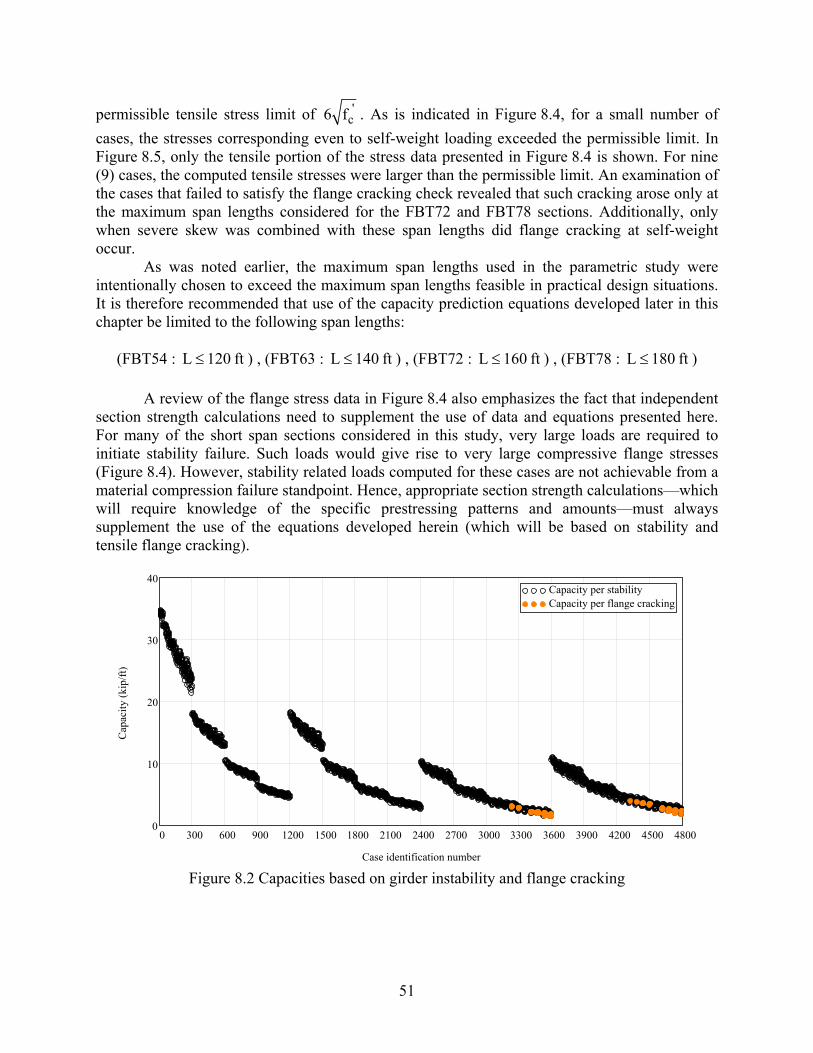
51
permissible tensile stress limit of 'c6 f . As is indicated in Figure 8.4, for a small number of
cases, the stresses corresponding even to self-weight loading exceeded the permissible limit. In Figure 8.5, only the tensile portion of the stress data presented in Figure 8.4 is shown. For nine (9) cases, the computed tensile stresses were larger than the permissible limit. An examination of the cases that failed to satisfy the flange cracking check revealed that such cracking arose only at the maximum span lengths considered for the FBT72 and FBT78 sections. Additionally, only when severe skew was combined with these span lengths did flange cracking at self-weight occur.
As was noted earlier, the maximum span lengths used in the parametric study were intentionally chosen to exceed the maximum span lengths feasible in practical design situations. It is therefore recommended that use of the capacity prediction equations developed later in this chapter be limited to the following span lengths:
(FBT54 : L 120 ft≤ ) , (FBT63 : L 140 ft≤ ) , (FBT72 : L 160 ft≤ ) , (FBT78 : L 180 ft≤ )
A review of the flange stress data in Figure 8.4 also emphasizes the fact that independent
section strength calculations need to supplement the use of data and equations presented here. For many of the short span sections considered in this study, very large loads are required to initiate stability failure. Such loads would give rise to very large compressive flange stresses (Figure 8.4). However, stability related loads computed for these cases are not achievable from a material compression failure standpoint. Hence, appropriate section strength calculations—which will require knowledge of the specific prestressing patterns and amounts—must always supplement the use of the equations developed herein (which will be based on stability and tensile flange cracking).
0 300 600 900 1200 1500 1800 2100 2400 2700 3000 3300 3600 3900 4200 4500 48000
10
20
30
40Capacity per stabilityCapacity per flange cracking
Case identification number
Cap
acity
(kip
/ft)
Figure 8.2 Capacities based on girder instability and flange cracking
52
0 300 600 900 1200 1500 1800 2100 2400 2700 3000 3300 3600 3900 4200 4500 48000
1
2
3
4
5Capacity per stabilityCapacity per flange cracking
Case identification number
Cap
acity
(kip
/ft)
Figure 8.3 Capacities for cases controlled by flange cracking
0 300 600 900 1200 1500 1800 2100 2400 2700 3000 3300 3600 3900 4200 4500 480025
20
15
10
5
0
5
Flange stresses correponding to computed capacities Flange stresses corresponding to girder self-weightMaximum permissible tensile stress
Case identification number
Stre
ss (k
si)
Figure 8.4 Computed flange stresses (Positive = tensile stress, negative = compressive stress)

53
0 300 600 900 1200 1500 1800 2100 2400 2700 3000 3300 3600 3900 4200 4500 48000
0.5
1
1.5Flange stresses correponding to computed capacities Flange stresses corresponding to girder self-weightMaximum permissible tensile stress
Case identification number
Stre
ss (k
si)
Figure 8.5 Computed tensile flange stresses
8.3.2 General trends
In Figure 8.6, the relationship between capacity and span length is presented for all 4800 cases analyzed. As span lengths increase, buckling capacities decrease rapidly (note that the vertical capacity axis in Figure 8.6 is a logarithmic scale). Given the nature of lateral buckling, this type of trend is generally expected, however, the figure also reveals a significant amount of variability (spread) in the capacity data at each span length. Part of this spread is clearly attributable to differences of cross-sectional properties across the various types of girders (FBT54, FBT63, FBT72, FBT78). However, other factors such as skew, slope, sweep, bearing pad creep, and bracing stiffness also contribute to the observed variability.
In Figure 8.7, an alternative view of capacity variability is given. In this figure, the influences of girder cross-section and span length have been removed, thereby revealing the combined (aggregate) influences of only skew, slope, sweep, bearing pad creep, and bracing stiffness. Each point in Figure 8.7 represents a particular girder type and span length under non-ideal conditions. Ideal conditions are defined here as zero-skew, zero-slope, minimal sweep, zero creep, and maximum bracing stiffness. For each non-ideal case, the corresponding ideal case for the same girder cross-section and span length is identified. The percentage change (reduction) in capacity resulting from non-ideal conditions is then computed as:
ideal non-ideal
ideal
C CΔC% = 100C
⎛ ⎞−⋅⎜ ⎟
⎝ ⎠ (8.1)
For each such calculation, the girder cross-sectional properties and span length match between the ideal and non-ideal cases, thus removing these as factors that might influence capacity. Figure 8.7 then illustrates buckling capacity variations attributable only to the effects of skew, slope, sweep, creep, and non-rigid bracing. Significant capacity reductions are apparent across the entire spectrum of girder types and span lengths considered.
54
80 100 120 140 160 180 2001
10
100
Span length (ft)
Cap
acity
(kip
/ft)
Figure 8.6 Variation of buckling capacity with span length
0 300 600 900 1200 1500 1800 2100 2400 2700 3000 3300 3600 3900 4200 4500 480010
0
10
20
30
40
50
Case identification number
Cap
acity
redu
ctio
n (%
)
Figure 8.7 Capacity reduction due to the combined effects of skew, slope,
sweep, creep, and non-rigid bracing
In Figures 8.8 and 8.9, capacity reductions are plotted according to girder types and span lengths. The observed ranges of capacity reduction are roughly uniform across all girder types and all span lengths. Therefore, in order to develop a better understanding of the individual factors that account for the observed capacity reductions, additional sensitivity studies were performed for the factors: skew, slope, sweep, creep, and bracing stiffness.
55
52 53 54 55 56 57 58 59 60 61 62 63 64 65 66 67 68 69 70 71 72 73 74 75 76 77 78 79 8010
0
10
20
30
40
50
Florida bulb-tee type (FBT54, FBT63, FBT72, FBT78)
Cap
acity
redu
ctio
n (%
)
Figure 8.8 Capacity reduction due to the combined effects of skew, slope, sweep, creep, and non-rigid bracing as a function of girder type
80 100 120 140 160 180 20010
0
10
20
30
40
50
Span length (ft)
Cap
acity
redu
ctio
n (%
)
Figure 8.9 Capacity reduction due to the combined effects of skew, slope,
sweep, creep, and non-rigid bracing as a function of span length
56
8.4 Parameter sensitivity studies
8.4.1 Sensitivity to creep
In the plots shown above in Figures 8.7– 8.9, the majority of data points correspond to positive values of capacity reduction. However, it is noted that there are also a smaller number of cases for which the computed capacity reductions are negative. A negative capacity “reduction” (i.e., a positive capacity increase), arises when the buckling capacity under non-ideal conditions exceeds the capacity under the so-called ideal conditions. In such cases, clearly the terms “ideal” and “non-ideal” lose their meaning.
By examining the sensitivity of buckling capacity to bearing pad creep, it is found that the cause of the negative capacity reductions in Figures 8.7 – 8.9 is primarily due to the effects of creep. Similar to the general capacity reduction Eqn. (8.1), we can define a reduction specifically for the effects of creep:
creep-excluded creep-included
creep-excluded
C CΔC% = 100
C⎛ ⎞−
⋅⎜ ⎟⎜ ⎟⎝ ⎠
(8.2)
Comparing Eqn. (8.2) to Eqn. (8.1), it is apparent that creep-excluded conditions are assumed to be ideal (reference) conditions. In Figure 8.10, capacity reductions associated with creep are plotted for a total of 2400 cases. In most cases, inclusion of creep results in a minor (less than 5%) reduction in buckling capacity. However, in a smaller number of cases, inclusion of creep actually results in a negative reduction—i.e., an increase in capacity.
Under conditions of combined skew and slope, the contact area between the bottom flange of the girder and the bearing pad is very small, resulting in very high localized stresses. If bearing pad creep is taken into account in such cases, the contact area between the girder and the bearing pad grows slightly over time as creep deformations occur. In some situations, this effect produces a minor net improvement (less than 5%) in buckling capacity. Overall, however, the conclusion to be drawn from Figure 8.10 is that, for the conditions studied here, girder buckling capacity is not highly sensitive to the inclusion, or exclusion, of bearing pad creep.
8.4.2 Sensitivity to skew
To evaluate the sensitivity of buckling capacity to skew angle, the following capacity reduction is defined:
zero-skew skewed
zero-skew
C CΔC% = 100C
⎛ ⎞−⋅⎜ ⎟⎜ ⎟
⎝ ⎠ (8.3)
Here, zero-skew conditions are considered to be ideal (reference) conditions and skewed conditions are considered to be non-ideal. In Figure 8.11, capacity reductions associated with skew angle are plotted for a total of 3840 cases. Sixteen distinct groups are apparent in the plot—four girder types at four different span lengths each. Maximum capacity reductions within each of these sixteen groups occur under the most severely skewed conditions. This fact is more

57
apparent in Figure 8.12 where the same 3840 capacity reductions are plotted as a function of skew angle. Plotting the data in this format, a clear linear trend between skew angle and reduction of buckling capacity becomes apparent. Later in this chapter, a simplified semi-empirical buckling capacity estimation equation will be developed based on the results of the overall parametric study. An important part of that simplified equation will be a skew correction factor that models the relationship between capacity loss and skew angle which is apparent in Figure 8.12.
0 300 600 900 1200 1500 1800 2100 2400 2700 3000 3300 3600 3900 4200 4500 480020
15
10
5
0
5
10
15
Case identification number
Cap
acity
redu
ctio
n (%
)
Figure 8.10 Capacity reduction due to creep
0 300 600 900 1200 1500 1800 2100 2400 2700 3000 3300 3600 3900 4200 4500 48005
0
5
10
15
20
25
30
35
40
Case identification number
Cap
acity
redu
ctio
n (%
)
Figure 8.11 Capacity reduction due to skew
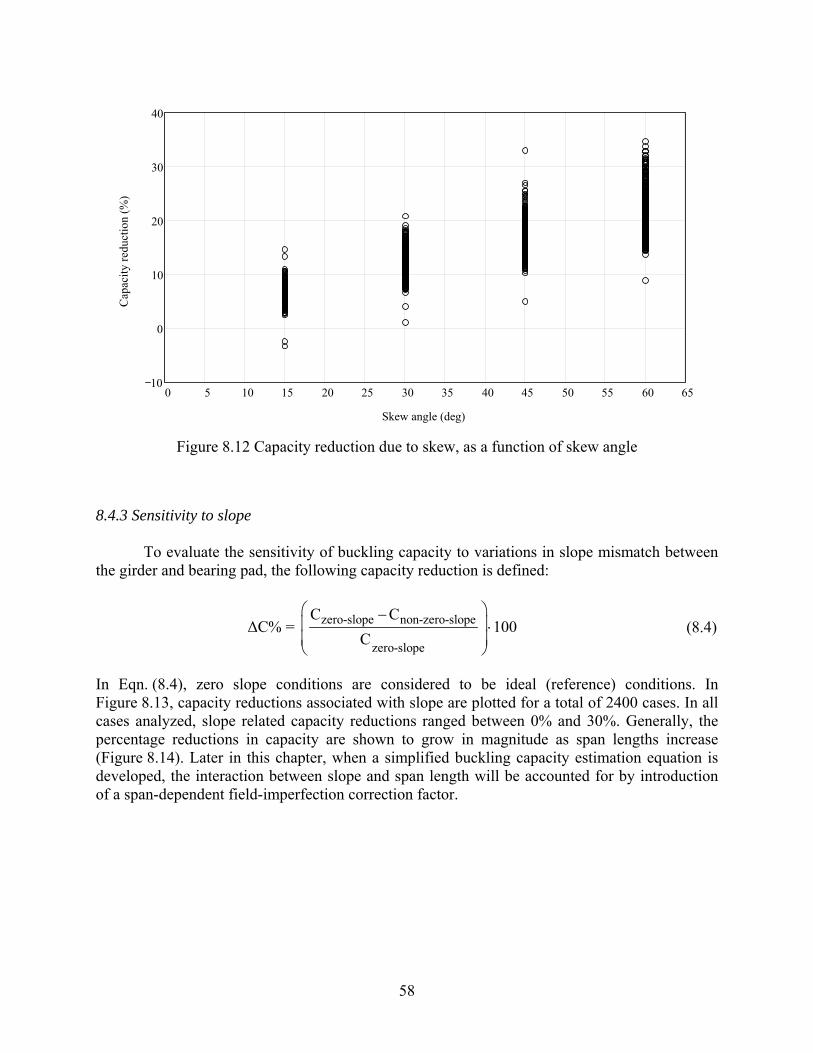
58
0 5 10 15 20 25 30 35 40 45 50 55 60 6510
0
10
20
30
40
Skew angle (deg)
Cap
acity
redu
ctio
n (%
)
Figure 8.12 Capacity reduction due to skew, as a function of skew angle
8.4.3 Sensitivity to slope
To evaluate the sensitivity of buckling capacity to variations in slope mismatch between the girder and bearing pad, the following capacity reduction is defined:
zero-slope non-zero-slope
zero-slope
C CΔC% = 100
C
⎛ ⎞−⎜ ⎟ ⋅⎜ ⎟⎝ ⎠
(8.4)
In Eqn. (8.4), zero slope conditions are considered to be ideal (reference) conditions. In Figure 8.13, capacity reductions associated with slope are plotted for a total of 2400 cases. In all cases analyzed, slope related capacity reductions ranged between 0% and 30%. Generally, the percentage reductions in capacity are shown to grow in magnitude as span lengths increase (Figure 8.14). Later in this chapter, when a simplified buckling capacity estimation equation is developed, the interaction between slope and span length will be accounted for by introduction of a span-dependent field-imperfection correction factor.
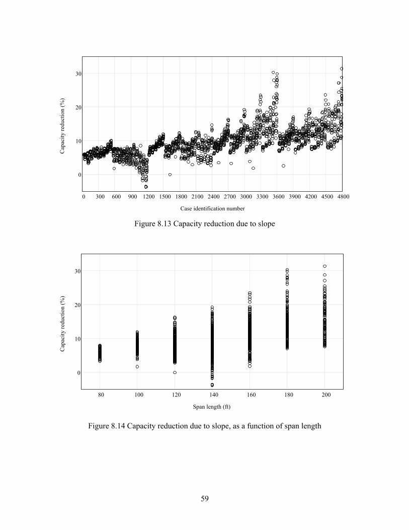
59
0 300 600 900 1200 1500 1800 2100 2400 2700 3000 3300 3600 3900 4200 4500 4800
0
10
20
30
Case identification number
Cap
acity
redu
ctio
n (%
)
Figure 8.13 Capacity reduction due to slope
80 100 120 140 160 180 200
0
10
20
30
Span length (ft)
Cap
acity
redu
ctio
n (%
)
Figure 8.14 Capacity reduction due to slope, as a function of span length

60
8.4.4 Sensitivity to sweep
To evaluate the sensitivity of buckling capacity to sweep imperfections, percentage capacity reductions were computed based on changes between minimum sweep (0.5 in.) and maximum sweep (2.5 in.) conditions. In this context, 0.5 in. sweep conditions were considered to be “ideal” conditions, whereas 2.5 in. sweep conditions were treated as non-ideal. Capacity reductions for sweep were then computed as:
0.5in. sweep 2.5 in. sweep
0.5 in. sweep
C CΔC% = 100
C
⎛ ⎞−⎜ ⎟ ⋅⎜ ⎟⎝ ⎠
(8.5)
In Figure 8.15, capacity reductions associated with slope are plotted for a total of 1600 cases. In nearly all cases analyzed, capacity reductions range between 0% and 25%. As was the case in slope-sensitivity, percentage reductions in capacity due to sweep are generally shown to grow in magnitude as span lengths increase (Figure 8.16). As noted above for slope-sensitivity, the interaction between sweep and span length will also be accounted for later in this chapter by introduction of a span-dependent field-imperfection correction factor.
0 300 600 900 1200 1500 1800 2100 2400 2700 3000 3300 3600 3900 4200 4500 480010
0
10
20
30
Case identification number
Cap
acity
redu
ctio
n (%
)
Figure 8.15 Capacity reduction due to sweep

61
80 100 120 140 160 180 20010
0
10
20
30
Span length (ft)
Cap
acity
redu
ctio
n (%
)
Figure 8.16 Capacity reduction due to sweep
8.4.5 Sensitivity to bracing stiffness
For a girder supported and braced only at its ends, ideal (maximum) buckling capacities are produced when rigid (infinitely stiff) braces are used. Capacity reductions resulting from non-ideal (non-rigid bracing) conditions may then be defined as:
rigid-bracing non-rigid-bracing
rigid-bracing
C CΔC% = 100
C
⎛ ⎞−⎜ ⎟ ⋅⎜ ⎟⎝ ⎠
(8.6)
In the parametric study conducted here, a bracing stiffness of 10,000 kip/in. was used to approximate rigid (ideal) bracing conditions. Capacity reductions associated with the use of non-rigid (non-ideal) bracing conditions were then computed in comparison to the pseudo-rigid (10,000 kip/in.) condition for the following bracing stiffness cases:
• Bracing stiffness case 0 : 0 kip/in. (unbraced) • Bracing stiffness case 1 : 10 kip/in. • Bracing stiffness case 2 : 100 kip/in. • Bracing stiffness case 3 : 1000 kip/in.
Results are presented in Figure 8.17 for a total of 3840 cases. Sixteen distinct groups are apparent in the plot—four girder types at four different span lengths each. Maximum capacity reductions within each of these sixteen groups occur under unbraced conditions. In Figure 8.18, capacity reductions for the same 3840 cases are grouped according to bracing stiffness case.
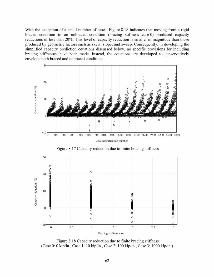
62
With the exception of a small number of cases, Figure 8.18 indicates that moving from a rigid braced condition to an unbraced condition (bracing stiffness case 0) produced capacity reductions of less than 20%. This level of capacity reduction is smaller in magnitude than those produced by geometric factors such as skew, slope, and sweep. Consequently, in developing the simplified capacity prediction equations discussed below, no specific provisions for including bracing stiffnesses have been made. Instead, the equations are developed to conservatively envelope both braced and unbraced conditions.
0 300 600 900 1200 1500 1800 2100 2400 2700 3000 3300 3600 3900 4200 4500 480010
0
10
20
30
Case identification number
Cap
acity
redu
ctio
n (%
)
Figure 8.17 Capacity reduction due to finite bracing stiffness
0 0.5 1 1.5 2 2.5 310
0
10
20
30
Bracing stiffness case
Cap
acity
redu
ctio
n (%
)
Figure 8.18 Capacity reduction due to finite bracing stiffness
(Case 0: 0 kip/in., Case 1: 10 kip/in., Case 2: 100 kip/in., Case 3: 1000 kip/in.)
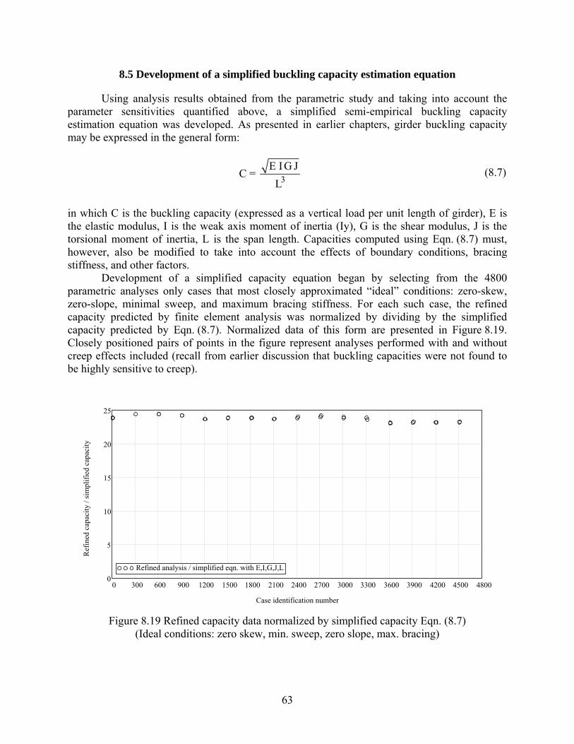
63
8.5 Development of a simplified buckling capacity estimation equation
Using analysis results obtained from the parametric study and taking into account the parameter sensitivities quantified above, a simplified semi-empirical buckling capacity estimation equation was developed. As presented in earlier chapters, girder buckling capacity may be expressed in the general form:
3E IG J
C = L
(8.7)
in which C is the buckling capacity (expressed as a vertical load per unit length of girder), E is the elastic modulus, I is the weak axis moment of inertia (Iy), G is the shear modulus, J is the torsional moment of inertia, L is the span length. Capacities computed using Eqn. (8.7) must, however, also be modified to take into account the effects of boundary conditions, bracing stiffness, and other factors.
Development of a simplified capacity equation began by selecting from the 4800 parametric analyses only cases that most closely approximated “ideal” conditions: zero-skew, zero-slope, minimal sweep, and maximum bracing stiffness. For each such case, the refined capacity predicted by finite element analysis was normalized by dividing by the simplified capacity predicted by Eqn. (8.7). Normalized data of this form are presented in Figure 8.19. Closely positioned pairs of points in the figure represent analyses performed with and without creep effects included (recall from earlier discussion that buckling capacities were not found to be highly sensitive to creep).
0 300 600 900 1200 1500 1800 2100 2400 2700 3000 3300 3600 3900 4200 4500 48000
5
10
15
20
25
Refined analysis / simplified eqn. with E,I,G,J,L
Case identification number
Ref
ined
cap
acity
/ si
mpl
ified
cap
acity
Figure 8.19 Refined capacity data normalized by simplified capacity Eqn. (8.7)
(Ideal conditions: zero skew, min. sweep, zero slope, max. bracing)
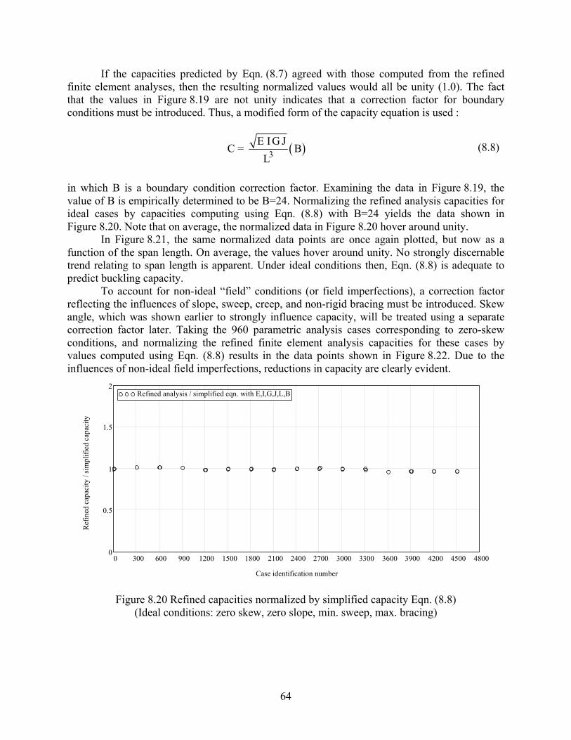
64
If the capacities predicted by Eqn. (8.7) agreed with those computed from the refined finite element analyses, then the resulting normalized values would all be unity (1.0). The fact that the values in Figure 8.19 are not unity indicates that a correction factor for boundary conditions must be introduced. Thus, a modified form of the capacity equation is used :
( )3E IG J
C = BL
(8.8)
in which B is a boundary condition correction factor. Examining the data in Figure 8.19, the value of B is empirically determined to be B=24. Normalizing the refined analysis capacities for ideal cases by capacities computing using Eqn. (8.8) with B=24 yields the data shown in Figure 8.20. Note that on average, the normalized data in Figure 8.20 hover around unity.
In Figure 8.21, the same normalized data points are once again plotted, but now as a function of the span length. On average, the values hover around unity. No strongly discernable trend relating to span length is apparent. Under ideal conditions then, Eqn. (8.8) is adequate to predict buckling capacity.
To account for non-ideal “field” conditions (or field imperfections), a correction factor reflecting the influences of slope, sweep, creep, and non-rigid bracing must be introduced. Skew angle, which was shown earlier to strongly influence capacity, will be treated using a separate correction factor later. Taking the 960 parametric analysis cases corresponding to zero-skew conditions, and normalizing the refined finite element analysis capacities for these cases by values computed using Eqn. (8.8) results in the data points shown in Figure 8.22. Due to the influences of non-ideal field imperfections, reductions in capacity are clearly evident.
0 300 600 900 1200 1500 1800 2100 2400 2700 3000 3300 3600 3900 4200 4500 48000
0.5
1
1.5
2Refined analysis / simplified eqn. with E,I,G,J,L,B
Case identification number
Ref
ined
cap
acity
/ si
mpl
ified
cap
acity
Figure 8.20 Refined capacities normalized by simplified capacity Eqn. (8.8) (Ideal conditions: zero skew, zero slope, min. sweep, max. bracing)
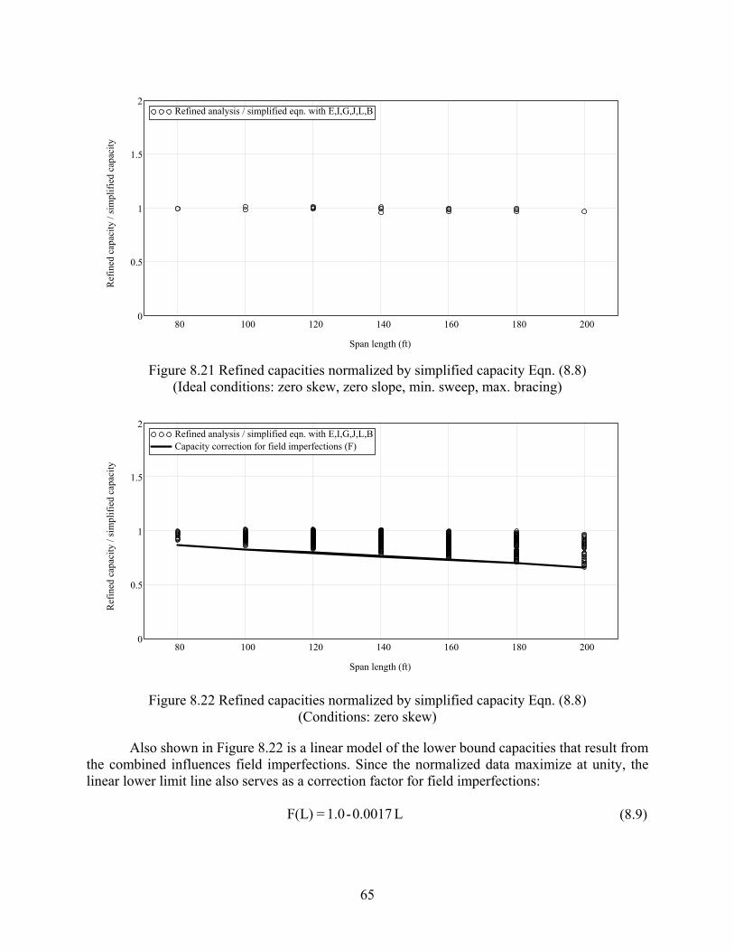
65
80 100 120 140 160 180 2000
0.5
1
1.5
2Refined analysis / simplified eqn. with E,I,G,J,L,B
Span length (ft)
Ref
ined
cap
acity
/ si
mpl
ified
cap
acity
Figure 8.21 Refined capacities normalized by simplified capacity Eqn. (8.8)
(Ideal conditions: zero skew, zero slope, min. sweep, max. bracing)
80 100 120 140 160 180 2000
0.5
1
1.5
2Refined analysis / simplified eqn. with E,I,G,J,L,B Capacity correction for field imperfections (F)
Span length (ft)
Ref
ined
cap
acity
/ si
mpl
ified
cap
acity
Figure 8.22 Refined capacities normalized by simplified capacity Eqn. (8.8) (Conditions: zero skew)
Also shown in Figure 8.22 is a linear model of the lower bound capacities that result from the combined influences field imperfections. Since the normalized data maximize at unity, the linear lower limit line also serves as a correction factor for field imperfections:
F(L) = 1.0-0.0017 L (8.9)
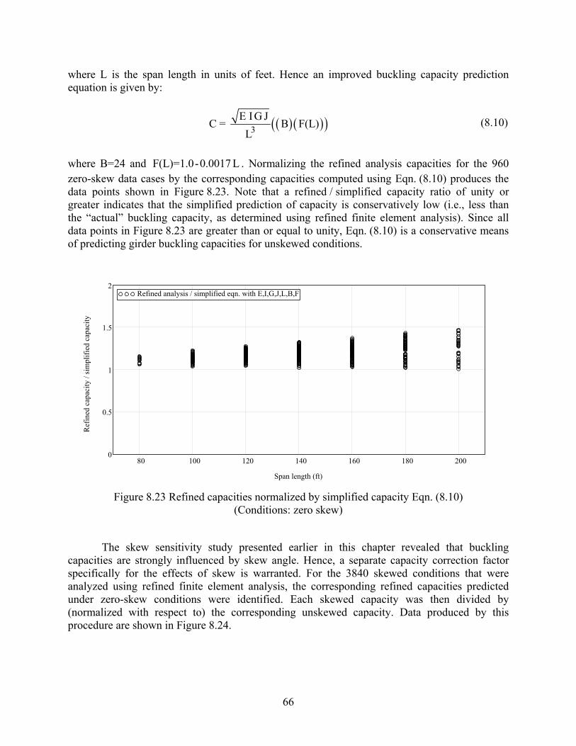
66
where L is the span length in units of feet. Hence an improved buckling capacity prediction equation is given by:
( ) ( )( )3E I G J
C = B F(L)L
(8.10)
where B=24 and F(L)=1.0-0.0017 L . Normalizing the refined analysis capacities for the 960 zero-skew data cases by the corresponding capacities computed using Eqn. (8.10) produces the data points shown in Figure 8.23. Note that a refined / simplified capacity ratio of unity or greater indicates that the simplified prediction of capacity is conservatively low (i.e., less than the “actual” buckling capacity, as determined using refined finite element analysis). Since all data points in Figure 8.23 are greater than or equal to unity, Eqn. (8.10) is a conservative means of predicting girder buckling capacities for unskewed conditions.
80 100 120 140 160 180 2000
0.5
1
1.5
2Refined analysis / simplified eqn. with E,I,G,J,L,B,F
Span length (ft)
Ref
ined
cap
acity
/ si
mpl
ified
cap
acity
Figure 8.23 Refined capacities normalized by simplified capacity Eqn. (8.10)
(Conditions: zero skew)
The skew sensitivity study presented earlier in this chapter revealed that buckling capacities are strongly influenced by skew angle. Hence, a separate capacity correction factor specifically for the effects of skew is warranted. For the 3840 skewed conditions that were analyzed using refined finite element analysis, the corresponding refined capacities predicted under zero-skew conditions were identified. Each skewed capacity was then divided by (normalized with respect to) the corresponding unskewed capacity. Data produced by this procedure are shown in Figure 8.24.
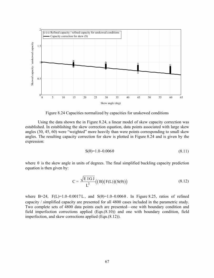
67
0 5 10 15 20 25 30 35 40 45 50 55 60 650
0.5
1
1.5
2Refined capacity / refined capacity for unskewed conditions Capacity correction for skew (S)
Skew angle (deg)
Skew
ed c
apac
ity /
unsk
ewed
cap
acity
Figure 8.24 Capacities normalized by capacities for unskewed conditions
Using the data shown the in Figure 8.24, a linear model of skew capacity correction was established. In establishing the skew correction equation, data points associated with large skew angles (30, 45, 60) were “weighted” more heavily than were points corresponding to small skew angles. The resulting capacity correction for skew is plotted in Figure 8.24 and is given by the expression:
S(θ)=1.0-0.006θ (8.11)
where θ is the skew angle in units of degrees. The final simplified buckling capacity prediction equation is then given by:
( ) ( ) ( )( )3E I G J
C = B F(L) S(θ)L
(8.12)
where B=24, F(L)=1.0-0.0017 L , and S(θ)=1.0-0.006θ . In Figure 8.25, ratios of refined capacity / simplified capacity are presented for all 4800 cases included in the parametric study. Two complete sets of 4800 data points each are presented—one with boundary condition and field imperfection corrections applied (Eqn.(8.10)) and one with boundary condition, field imperfection, and skew corrections applied (Eqn.(8.12)).
68
0 300 600 900 1200 1500 1800 2100 2400 2700 3000 3300 3600 3900 4200 4500 48000
0.5
1
1.5
2
Refined analysis / simplified eqn. with E,I,G,J,L,B,F Refined analysis / simplified eqn. with E,I,G,J,L,B,F,S
Case identification number
Ref
ined
cap
acity
/ si
mpl
ified
cap
acity
Figure 8.25 Refined capacities normalized by simplified capacity Eqn. (8.10) without
skew correction, and normalized by Eqn. (8.12) with skew correction
When all three capacity corrections are included—boundary condition, field imperfection, and skew—the refined / simplified capacity ratios are greater than or equal to unity. Thus, the equation:
( ) ( )3E I G J
C = 24 1.0-0.0017 L 1.0-0.006θL
(8.13)
where L is the span length in units of feet and θ is the skew angle in units of degrees, is found to be a conservative predictor of girder buckling capacity for the full range of girder type, span length, skew angle, slope, sweep, creep, and bracing conditions studied here. In Figure 8.26, girder buckling capacities computed using by simplified Eqn. (8.13) and by refined finite element analysis are compared. Evident from the figure is the fact that the simplified equation is always conservative, and matches the trends present in the refined analysis data set. This is further illustrated in Figure 8.27 where the same data are compared, but only within the range from 1 kip/ft to 10 kip/ft and using a logarithmic vertical scale. In this figure, it is clear that the simplified equation is conservative for every analysis case considered.
Eqn. (8.13) is therefore recommended for use in assessing girder buckling capacity for Florida bulb-tee sections, subject to the following, previously discussed, limiting span lengths:
(FBT54 : L 120 ft≤ ) , (FBT63 : L 140 ft≤ ) , (FBT72 : L 160 ft≤ ) , (FBT78 : L 180 ft≤ )
As was noted earlier, capacities predicted by Eqn. (8.13) are based on the conditions of overall girder stability and flange tension cracking. However, the potential for other failure conditions

69
(e.g. flange crushing in compression) may also exist. Therefore, appropriate section strength calculations—which will require knowledge of the specific prestressing patterns and amounts—must always supplement the use of Eqn. (8.13).
0 300 600 900 1200 1500 1800 2100 2400 2700 3000 3300 3600 3900 4200 4500 48000
10
20
30
40Refined analysis Simplified eqn. with E,I,G,J,L,B,F,S
Case identification number
Cap
acity
(kip
/ft)
Figure 8.26 Comparison of capacities computed by refined analysis and by simplified capacity Eqn. (8.13)
0 300 600 900 1200 1500 1800 2100 2400 2700 3000 3300 3600 3900 4200 4500 48001
10
Refined analysis Simplified eqn. with E,I,G,J,L,B,F,S
Case identification number
Cap
acity
(kip
/ft)
Figure 8.27 Comparison of capacities computed by refined analysis and by simplified capacity Eqn. (8.13)
70
CHAPTER 9 WIND LOAD ANALYSIS PROCEDURES
9.1 Introduction
By modifying the vertical-load buckling analysis techniques described in previous chapters, it was feasible to carry out an investigation into the effects of lateral wind loading on long span girders. The wind loading investigation was limited in scope and preliminary in nature, but was carried out with the goal of gaining insights into girder behavior and stability under lateral loading conditions. It is important to note that material failure limit states (e.g., weak-axis flexural failure, flange cracking, etc.) were not included in this investigation, therefore the results obtained from this part of the study were not conclusive in nature. Additionally, only unbraced conditions were analyzed for wind loading. Hence, the focus was primarily on girder stability against rollover in free-standing (no lateral bracing) conditions.
9.2 Wind loading system model
Florida bulb-tee girder types FBT54, FBT63, FBT72 and FBT78 were analyzed under various combinations of span length, skew angle, slope, and sweep for the purpose of assessing girder stability and quantifying wind loading capacities. Bearing pad behavior was represented using the simplified bearing pad model described in previous chapters. The ability of the simplified pad model to represent girder lift-off—discussed earlier—is particularly important in the analysis of girder overturning under lateral wind loading. Wind loads were applied to the girder as uniformly distributed line loads that acted in such a manner as to increase girder sweep (Figure 9.1). The loading procedure consisted of two stages: 1) ramping the vertical load to the self-weight of girder and, 2) while holding the vertical self-weight load constant, ramping the lateral wind load up from zero until girder instability occurred (Figure 9.2).
Rigid grid
X
Y
SweepGirder elements
Lateral wind load
X
ZWind load
Vertical load
Figure 9.1 Wind loading system model

71
Prior to application of any load, ten stabilizing linear springs were provided at each end
of the girder (as discussed in previous chapters). The stabilization springs were gradually removed from the analysis as the vertical load acting on the girder increased. Upon reaching the full girder self-weight load, all stabilization braces were removed. From this point in time forward, vertical load was held constant while lateral wind load was linearly increased. The analysis terminated when girder rollover occurred.
w selfweight
Vertical load
Time
Lateral wind load
Time
Number of stabilization springs active at each end of girder model
10 9 8 7 6 5 4 3 2 1 0 0
Number of stabilization springs active at each end of girder model
10 9 8 7 6 5 4 3 2 1 0 0
30 sec. self-weight loading
Figure 9.2 Load application procedure used for wind loading analysis
9.3 Validation of wind loading analysis procedure
As was the case in the vertical buckling load analyses discussed in previous chapters, stability analyses under lateral wind loading conditions were carried out using the large-displacement analysis procedure. To validate that the simplified bearing pad model and the large displacement analysis technique could properly predict girder overturning, the system model was modified to represent an infinitely stiff girder sitting on rigid supports. For an infinitely stiff girder, flexural deformation of the girder does not occur and the problem reduces to a simple static equilibrium problem (Figure 9.3),. The magnitude of wind loading that causes girder overturning can then be determined as follows:
72
( ) ( ) ( )( )pivot wind self-weight bM = w y - w L /2 0=∑
( )( ) ( ) ( )( )pivot wind self-weight bM = p H y - w L /2 0=∑
( )( )( ) ( )
self-weight bwind
w L /2p
H y=
(9.1)
In this equation, windp is wind loading expressed as a pressure (force/area), self-weightw is the girder self-weight (force/length), H is the girder height, y is the elevation of the girder centroid, and bL is the width of the rigid bearing pad.
wself-weight
wwind
H
Pivot point
Lb
X
Z
y_
pwind
Figure 9.3 Rigid-girder wind capacity determination based on equilibrium
Skew, slope, sweep and creep were excluded from the validation analyses. To approximate the rigid girder and rigid bearing conditions, the Young’s modulus of the concrete girder and the stiffness of the truss elements representing the bearing pad were increased to 100 times their normal values. Four Florida bulb-tee girders having varying span lengths were analyzed for wind-induced overturning: an 80 ft. FBT54, a 100 ft. FBT63, a 120 ft. FBT72, and a 140 ft. FBT78. Results obtained from Eqn. (9.1) and from ADINA large displacement analyses are compared in Figures 9.4 through 9.7. In each case, the ADINA predictions of wind load required to initiate overturning are in good agreement with the value obtained from static equilibrium.
73
Lateral girder displacement at midspan (ft)
Win
d lo
ad (p
sf)
0 0.005 0.01 0.015 0.02 0.025 0.03 0.035 0.04 0.045 0.05 0.055 0.06 0.0650
10
20
30
40
50
60
70
80
90
Girder overturning
ADINA analysis solutionMoment equilibrium solution
Figure 9.4 Validation wind loading analysis (FBT54, 80 ft. span)
Lateral girder displacement at midspan (ft)
Win
d Lo
ad (p
sf)
0 0.005 0.01 0.015 0.02 0.025 0.03 0.035 0.04 0.045 0.05 0.055 0.06 0.065 0.07 0.075 0.080
5
10
15
20
25
30
35
40
45
50
55
60
65
70
Girder overturning
ADINA analysis solutionMoment equilibrium solution
Figure 9.5 Validation wind loading analysis (FBT63, 100 ft. span)
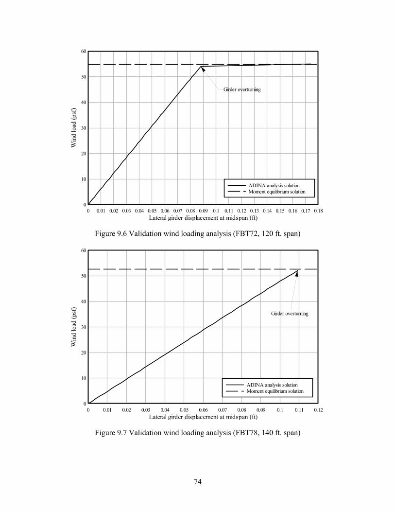
74
Lateral girder displacement at midspan (ft)
Win
d lo
ad (p
sf)
0 0.01 0.02 0.03 0.04 0.05 0.06 0.07 0.08 0.09 0.1 0.11 0.12 0.13 0.14 0.15 0.16 0.17 0.180
10
20
30
40
50
60
Girder overturning
ADINA analysis solutionMoment equilibrium solution
Figure 9.6 Validation wind loading analysis (FBT72, 120 ft. span)
Lateral girder displacement at midspan (ft)
Win
d lo
ad (p
sf)
0 0.01 0.02 0.03 0.04 0.05 0.06 0.07 0.08 0.09 0.1 0.11 0.120
10
20
30
40
50
60
Girder overturning
ADINA analysis solutionMoment equilibrium solution
Figure 9.7 Validation wind loading analysis (FBT78, 140 ft. span)
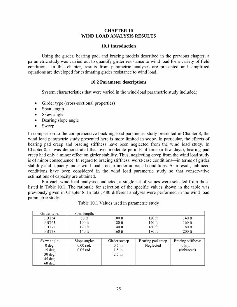
75
CHAPTER 10 WIND LOAD ANALYSIS RESULTS
10.1 Introduction
Using the girder, bearing pad, and bracing models described in the previous chapter, a parametric study was carried out to quantify girder resistance to wind load for a variety of field conditions. In this chapter, results from parametric analyses are presented and simplified equations are developed for estimating girder resistance to wind load.
10.2 Parameter descriptions
System characteristics that were varied in the wind-load parametric study included:
• Girder type (cross-sectional properties) • Span length • Skew angle • Bearing slope angle • Sweep
In comparison to the comprehensive buckling-load parametric study presented in Chapter 8, the wind load parametric study presented here is more limited in scope. In particular, the effects of bearing pad creep and bracing stiffness have been neglected from the wind load study. In Chapter 8, it was demonstrated that over moderate periods of time (a few days), bearing pad creep had only a minor effect on girder stability. Thus, neglecting creep from the wind load study is of minor consequence. In regard to bracing stiffness, worst-case conditions—in terms of girder stability and capacity under wind load—occur under unbraced conditions. As a result, unbraced conditions have been considered in the wind load parametric study so that conservative estimations of capacity are obtained.
For each wind load analysis conducted, a single set of values were selected from those listed in Table 10.1. The rationale for selection of the specific values shown in the table was previously given in Chapter 8. In total, 480 different analyses were performed in the wind load parametric study.
Table 10.1 Values used in parametric study
Girder type: Span length: FBT54 80 ft 100 ft 120 ft 140 ft FBT63 100 ft 120 ft 140 ft 160 ft FBT72 120 ft 140 ft 160 ft 180 ft FBT78 140 ft 160 ft 180 ft 200 ft
Skew angle: Slope angle: Girder sweep Bearing pad creep Bracing stiffness:
0 deg. 0.00 rad. 0.5 in. Neglected 0 kip/in 15 deg. 0.05 rad. 1.5 in. (unbraced) 30 deg. 2.5 in. 45 deg. 60 deg.
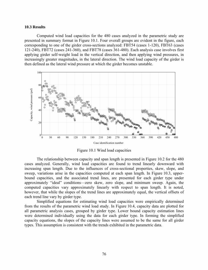
76
10.3 Results
Computed wind load capacities for the 480 cases analyzed in the parametric study are presented in summary format in Figure 10.1. Four overall groups are evident in the figure, each corresponding to one of the girder cross-sections analyzed: FBT54 (cases 1-120), FBT63 (cases 121-240), FBT72 (cases 241-360), and FBT78 (cases 361-480). Each analysis case involves first applying girder self-weight load in the vertical direction, and then applying wind pressures, in increasingly greater magnitudes, in the lateral direction. The wind load capacity of the girder is then defined as the lateral wind pressure at which the girder becomes unstable.
0 30 60 90 120 150 180 210 240 270 300 330 360 390 420 450 4800
20
40
60
80
100
Case identification number
Cap
acity
, win
d pr
essu
re (p
sf)
Figure 10.1 Wind load capacities
The relationship between capacity and span length is presented in Figure 10.2 for the 480 cases analyzed. Generally, wind load capacities are found to trend linearly downward with increasing span length. Due to the influences of cross-sectional properties, skew, slope, and sweep, variations arise in the capacities computed at each span length. In Figure 10.3, upper-bound capacities, and the associated trend lines, are presented for each girder type under approximately “ideal” conditions—zero skew, zero slope, and minimum sweep. Again, the computed capacities vary approximately linearly with respect to span length. It is noted, however, that while the slopes of the trend lines are approximately equal, the vertical offsets of each trend line vary by girder type.
Simplified equations for estimating wind load capacities were empirically determined from the results of the parametric wind load study. In Figure 10.4, capacity data are plotted for all parametric analysis cases, grouped by girder type. Lower bound capacity estimation lines were determined individually using the data for each girder type. In forming the simplified capacity equations, the slopes of the capacity lines were assumed to be the same for all girder types. This assumption is consistent with the trends exhibited in the parametric data.
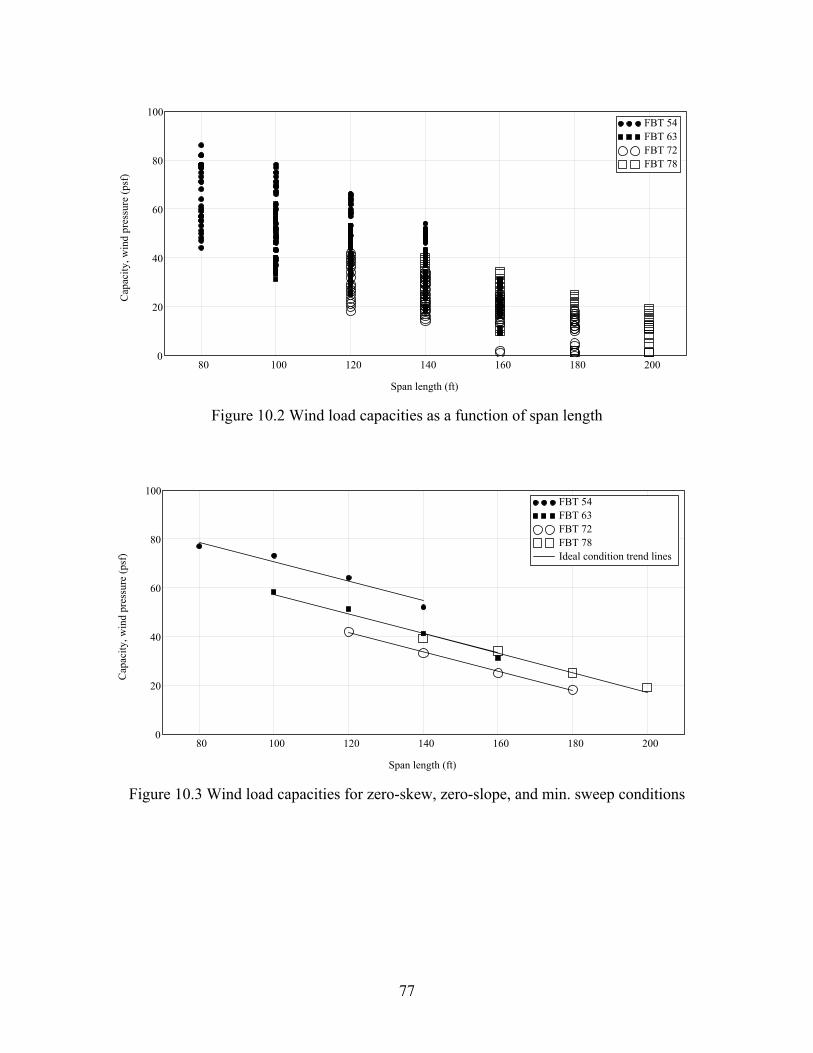
77
80 100 120 140 160 180 2000
20
40
60
80
100FBT 54FBT 63FBT 72FBT 78
Span length (ft)
Cap
acity
, win
d pr
essu
re (p
sf)
Figure 10.2 Wind load capacities as a function of span length
80 100 120 140 160 180 2000
20
40
60
80
100FBT 54FBT 63FBT 72FBT 78Ideal condition trend lines
Span length (ft)
Cap
acity
, win
d pr
essu
re (p
sf)
Figure 10.3 Wind load capacities for zero-skew, zero-slope, and min. sweep conditions
78
80 100 120 140 160 180 2000
10
20
30
40
50
60
70FBT 54Limit
Span length (ft)
Cap
acity
, win
d pr
essu
re (p
sf)
80 100 120 140 160 180 2000
10
20
30
40
50
60
70FBT 63Limit
Span length (ft)
Cap
acity
, win
d pr
essu
re (p
sf)
80 100 120 140 160 180 2000
10
20
30
40
50
60
70FBT 72Limit
Span length (ft)
Cap
acity
, win
d pr
essu
re (p
sf)
80 100 120 140 160 180 2000
10
20
30
40
50
60
70FBT 78Limit
Span length (ft)
Cap
acity
, win
d pr
essu
re (p
sf)
Figure 10.4 Simplified wind load capacity estimation curves for each girder type

79
A conservative, lower-bound model of wind load capacity was determined to be of the form:
( )C = 0.4 L0- L (10.1)
Here C is the wind load capacity (in units of psf), L is the span length (in units of ft), and L0 is the span length (in units of ft) at which the wind load capacity reaches zero. Values of L0 vary by girder type and are listed in Table 10.2.
Table 10.2 Parameters L0 for each girder type
Girder type: L0 (ft)
FBT54 190 FBT63 178 FBT72 162 FBT78 182
80
CHAPTER 11 CONCLUSIONS AND RECOMMENDATIONS
11.1 Conclusions
This study was undertaken primarily for the purposes of investigating the lateral stability of long-span prestressed concrete girders—specifically Florida bulb-tee girders—during bridge construction and offering recommendations for improving such stability. Numerical analysis techniques and limited experimental testing were used to quantify girder buckling capacities and wind load capacities as functions of girder cross-sectional properties, span length, bridge skew angle, bracing stiffness, and factors representing field conditions (sweep imperfections, slope mismatches, and bearing pad creep). Based on results obtained from parametric studies the following conclusions are drawn:
1. Girder stability and buckling capacity are strongly influenced by cross-sectional properties
and span length—both well understood factors—and by the interaction of skew and slope at the girder bearings. The camber level in prestressed concrete bridge girders is typically set so as to offset the effects of deflection due to the dead load of the bridge deck. However, when a girder is first placed onto its bearings, only girder self-weight load acts. As a result, the ends of the girder may be sloped (vertically rotated) relative to the surface of the bearing pads. Factors such as bridge grade and construction tolerances can also add to slope mismatches between the girder and bearing pad. When a bearing pad is skewed relative to the longitudinal axis of the girder, slope and skew combine to produce a condition in which contact between the girder and pad is localized to a single corner of the pad:
Skewangle
Support
Girder
Bearingpad
Area of lowerbearing pressure
Roll stiffnessof bearing pad
Roll stiffnessof bearing pad
Unskewed condition Skewed condition
Area of higherbearing pressure
The resulting asymmetric and non-uniform distribution of bearing pressure significantly reduces the rotational (“roll”) resistance that the pad provides to the girder. As a result, girder buckling capacities under such conditions are significantly reduced in comparison to unskewed conditions. It is noted that once deck dead load is applied to the girder, the slope mismatch between the girder and pad will be reduced as the girder deflects and the ends rotate. Hence, capacity reductions associated with the effects of skew and slope are at their worst when a girder is resting on its bearings and carrying only self-weight load.
81
2. Over moderate durations of time (a few days), bearing pad creep appears to have only a
minor effect on girder stability and buckling capacity. Buckling capacities computed with creep effects included differed only by about 5% in comparison to capacities computed with creep effects excluded. In some situations, creep produced a small loss of capacity, while in other situations, creep actually increased capacity slightly. On average, however, girder buckling capacity was not found to be strongly influenced by moderate term bearing pad creep.
3. In bridges with skewed geometry, the use of end-point bracing increases girder buckling
capacities, however, greater increases in capacity can be achieved by reducing the adverse effects of combined skew and slope. Smaller capacity increases can be achieved by moving from an unbraced condition to a rigidly braced condition than can be achieved by eliminating skew between the girder and pad.
11.2 Recommendations
Based on the results obtained from this research, the following recommendations are offered: 1. Unless more refined analysis methods are available, it is recommended that the following
equation be used to evaluate the influence that field conditions and skew angle have on girder buckling capacity:
( ) ( )3E I G J
C = 24 1.0-0.0017 L 1.0-0.006θL
In the equation above, C is the maximum uniform distributed load that a girder can carry (in units of kip/ft), E is the elastic modulus of concrete (in units of kip/ft2), I is the weak axis moment of inertia of the girder (in units of ft4), G is the shear modulus of concrete (in units of kip/ft2), J is the torsional constant for the girder (in units of ft4), L is the span length (in units of feet), and θ is the skew angle between the bearing pads and the longitudinal axis of the girder (in units of degrees). Capacities predicted by the above equation are based on limit states related to lateral buckling (girder stability) and tensile flange stresses (cracking). Additional section capacity calculations based on alternative failures modes (e.g., compression failure in the flange, etc.) should always supplement use of the equation given above. Based on the results of flange tension cracking checks that were performed, it is recommended that use of the equation given above be limited in application to the following span lengths: (FBT54 : L 120 ft≤ ) , (FBT63 : L 140 ft≤ ) , (FBT72 : L 160 ft≤ ) , (FBT78 : L 180 ft≤ )
2. It is recommended that consideration be given to requiring bearing pads in long span prestressed concrete girder bridges to be oriented to match girder alignment and thereby eliminate the adverse effects of skew (at least from the perspective of girder stability during
82
the construction process). By aligning the bearing pads with the longitudinal girder axis, greater roll resistance is provided to the girder.
Skewangle
Support
Girder
Bearingpad
Roll stiffnessof bearing pad
Skewangle
Roll stiffnessof bearing pad
Bearing pad skewed relative to girder Bearing pad unskewed relative to girder
Given that slope mismatches between girder and pad, due camber and bridge grade, are essentially unavoidable, eliminating the adverse effects of skew at the girder-pad contact zone is highly desirable and would yield improved girder stability.
3. Further research should be conducted to experimentally verify the analytically-obtained
results presented in this report. Experimental verification testing should include, at a minimum, girder tests performed for the purpose of assessing lateral girder buckling loads. In addition, experimental determination of bearing pad roll stiffness under conditions of combined skew and slope should be considered for investigation.
4. None of the capacity prediction equations presented in this report include an explicitly
chosen factor of safety. In addition, the proposed capacity prediction equations have not yet been experimentally validated. It is therefore recommended that future research be conducted to rationally select appropriate factors of safety. Additionally, until such work is completed, it is recommended that factors of safety of not less then 3.0 be used in conjunction with the equations presented here.
5. In the present study, the use of bracing only at the girder end-points has been evaluated.
Additional analytical and/or experimental investigations should be carried out to quantify the effectiveness of bracing schemes that use end-point and intermediate braces to tie multiple girders together as a system.
6. Further research is needed to adequately address the issue of predicting girder stability and
strength under lateral wind loading conditions.
83
REFERENCES AASHTO (2004), LRFD Bridge Design Specifications, American Association of State Highway
and Transportation Officials, Washington, D.C.
ACI (2005), ACI 318-05: Building Code Requirements for Structural Concrete and Commentary, American Concrete Institute.
ADINA (2005), Theory and Modeling Guide, Volume I: ADINA Solids & Structures, ADINA R&D, Inc.
Allen H.G, and Bulson P.S. (1980), Background to Buckling, McGraw-Hill, London.
Anderson A.R. (1971), “Lateral Stability of Long Prestressed Concrete Beams” PCI Journal, Vol. 16, pp. 7-9.
FDOT (2005), “FDOT Standard Drawings”, Structures Design Office, Florida Department of Transportation, Tallahassee, FL.
FDOT (2006), “FDOT Design Standards”, Structures Design Office, Florida Department of Transportation, Tallahassee, FL.
FDOT (2006), “FDOT Structures Design Guidelines”, Structures Design Office, Florida Department of Transportation, Tallahassee, FL.
FDOT (1991), “FDOT Standard Specifications for Road and Bridge Construction”, Florida Department of Transportation, Tallahassee, FL.
Flint, A.R. (1951), “The Influence of Restraints on The Stability of Beams”, Structural Engineer, Vol. 29, pp. 235-246.
Gent, A.N (2001), “Engineering with Rubber – How to Design Rubber Components”, 2nd Ed., HanserGardner Publications, Inc., Cincinnati, Ohio.
Laszlo, G. and Imper, R.R. (1987), “Handling and Shipping of Long Span Bridge Beams”, PCI Journal, Vol. 32, pp. 86-101.
Mast, R.F (1989), “Lateral Stability of Long Prestressed Concrete Beams” Part I, PCI Journal, Vol 34, pp. 34-53.
Mast, R.F (1993), “Lateral Stability of Long Prestressed Concrete Beams” Part II, PCI Journal, Vol 38, pp. 70-88.
Mast, R.F (1994), “Lateral Bending Test to Destruction of a 149ft Prestressed Concrete I-Beam”, PCI Journal, Vol. 39, pp. 54-62.
Muller, J. (1962), “Lateral Stability of Precast Members During Handling and Placing”, PCI Journal, Vol. 7, pp. 21-31.

84
Nethercot, D.A. and Rockey, K.C. (1972), “The Lateral Buckling of Beam Having Discrete Intermediate Restraints”, The Structural Engineer, Vol.50, No. 10, pp. 391-403.
Nethercot, D.A (1973), “Buckling of Laterally or Torsionally Restrained Beams”, Journal of the Engineering Mechanics Division, ASCE, Vol. 99, No EM4, Proc. Paper 9903, pp.773-791.
PCI (2003), “PCI Bridge Design Manual”, Precast/Prestressed Concrete Institute, Chicago, IL.
PCI (1999), “PCI Manual 116-99: Quality Control for Plants and Production of Structural Precast Concrete Products”, Precast/Prestressed Concrete Institute, Chicago, IL.
Schmidt, L.C. (1965), “Restraints Against Elastic Lateral Buckling” Journal of the Engineering Mechanics Division, ASCE, Vol. 91, No EM6, Proc. Paper 4561, pp.1-10.
Stratford, T.J. and Burgoyne, C.J. (1999), “Lateral Stability of Long Precast Concrete Beams”, Proceedings of the Institution of Civil Engineers – Structures and Buidings, Vol. 124, pp. 169-180.
Stratford, T.J. and Burgoyne, C.J. (1999), “Stability Design of Long Precast Concrete Beams”, Proceedings of the Institution of Civil Engineers – Structures and Buidings, Vol. 134, pp. 159-168.
Stratford, T.J. and Burgoyne, C.J. (2000), “The Toppling of Hanging Beams”, International Journal of Solids and Structure, Vol. 37, pp. 3569-3589.
Stratford, T.J. and Burgoyne, C.J. (2001), “Lateral Stability of Long-Span Prestressed Concrete Beams on Flexible bearings”, The structural Engineer, Vol. 79, No6, pp. 23-26.
Timoshenko S.P., Goodier, J.N. (1970), Theory of Elasticity, 3rd Ed., McGraw-Hill, New York.
Trahair, N.S. (1977), The Behaviour and Design of Steel Structures, Chapman and Hall, London.
Trahair N.S. (1993), Flexural-Torsional Buckling of Structures, E. & F.N. Spon, London.
Treloar L.R.G (1944), “Stress-Strain Data for Vulcanized Rubber Under Various Types of Deformations”, Trans. Faraday Soc., Vol. 40, pp.59-70.
Yazdani, N., Eddy, S., and Cai, C.S (2000),”Effect of Bearing Pads on Precast Prestressed Concrete Bridges”, Journal of Bridge Engineering, Vol. 5, Issue. 3, pp. 224-232.
Young, W.C. (1989), Roark’s Formulas for Stress and Strain, 6th Ed., McGraw-Hill, New York.
Yura, J et al. (2001), Elastomeric Bridge Bearings: Recommended Test Methods, NCHRP Report No. 449, Washington D.C.
85
APPENDIX A APPROXIMATE CALCULATION OF TORSIONAL CONSTANT
Accurate determination of torsional constants requires the use of relatively sophisticated
numerical approaches that generally employ the “pressurized membrane analogy” of torsion (Young 1989 article 4.4 and 9.2, Timoshenko and Goodier 1970 article 107). Such methods require that the shape of the cross-section be carefully discretized (meshed) and analyzed using computer software.
In lieu of conducting this type of analysis, a variation on a procedure outlined in ACI 318-05 (ACI 2005) may be used to estimate torsional constants for girder cross-sections. In Chapter 13 of ACI 318-05, the following expression is given for estimating the torsional constant of a section consisting of rectangular shapes:
In this equation, x is the shorter overall dimension of each rectangle, and y is the longer overall dimension. To apply Eqn. A.1 to an I-shaped girder, it is recommended that the cross-section be divided into three distinct parts: top flange, web, and bottom flange. Note that subdivision of the cross-section into a larger number of smaller parts will generally worsen, not improve, the estimation of torsional constant when applying Eqn. A.1. The procedure recommended here for subdividing a section is illustrated in Figure A.1 for an FBT78 section. The widths of the rectangles are set equal to the overall dimensions of the corresponding parts in the actual cross-section. The vertical heights of the rectangles are then computed to make the part-areas match between the true cross-sectional shape, and the piecewise rectangular shape.
10.5"
8 in.
10 in.
78 in.
3 in.
3 in.60 in.
7 in.
3 in.4 in.
28 in.
50 in.
60 in.
28 in.
5.933 in.
7 in.
14.25 in.
A=356 in2
A=399 in2
A=3
50 in
2
A=356 in2
A=3
50 in
2
A=399 in2
Figure A.1 Actual FBT78 cross-section (left) and recommended
equivalent piecewise rectangular cross-section (right)
3x x yJ = 1 - 0.63y 3
⎛ ⎞⎛ ⎞⎜ ⎟⎜ ⎟
⎝ ⎠⎝ ⎠∑ (A.1)
86
In Figure A.2, the calculations involved in approximating the torsional constant for an FBT78 girder are shown. Results obtained from approximate torsional calculations for the bulb-tee girders considered in this study are summarized and compared to exact values in Table A.1. In each case, the approximated torsional constant is less than the corresponding exact torsional constant. Consequently, use of the approximate torsional constants in buckling capacity calculations will yield conservative under-predictions of girder strength.
Calculation of approximate torsional constant for an FBT78 girder
Torsional constant estimation equation (ACI 318-05 Chapter 13) ...
J x y,( ) 1 0.63xy
⎛⎜⎝
⎞⎟⎠
−⎡⎢⎣
⎤⎥⎦
x3 y⋅3
⋅:=
Equivalent rectangle for top flange ...
A1 60 in⋅( ) 3 in⋅( )⋅ 0.5( ) 60 in⋅ 13 in⋅+( )⋅ 4 in⋅( )⋅+ 0.5( ) 13 in⋅ 7 in⋅+( )⋅ 3 in⋅( )⋅+:= A1 356 in2=
y1 60 in⋅:= ... longer dimension of rectangle is width of top flange
x1 A1 y1÷:= x1 5.933 in=
J1 J x1 y1,( ):= J1 3917 in4=
Equivalent rectangle for web ...
A2 7 in⋅( ) 50 in⋅( )⋅:= A2 350 in2=
y2 50 in⋅:= ... longer dimension of rectangle is height of constant-width web
x2 A2 y2÷:= x2 7 in=
J2 J x2 y2,( ):= J2 5212 in4=
Equivalent rectangle for bottom flange ...
A3 0.5( ) 7 in⋅ 28 in⋅+( )⋅ 10 in⋅( )⋅ 28 in⋅( ) 8 in⋅( )⋅+:= A3 399 in2=
y3 28 in⋅:= ... longer dimension of rectangle is width of bottom flange
x3 A3 y3÷:= x3 14.25 in=
J3 J x3 y3,( ):= J3 18348 in4=
Summary ...
Part number Part name x y J
1 Top flange x1 5.933 in= y1 60 in= J1 3917 in4=
2 Web x2 7 in= y2 50 in= J2 5212 in4=
3 Bottom flange x3 14.25 in= y3 28 in= J3 18348 in4=
Japprox J1 J2+ J3+:=
Japprox 27478 in4=
Approximation error ...
Jexact 35270 in4⋅:= ... obtained from refined numerical analysis
errorJexact Japprox−
Jexact100⋅:=
error 22.1= %
Figure A.2 Calculation of approximate torsional constant for an FBT78 girder
87
Table A.1 Comparison of exact and approximate torsional constants
Girder type:
Exact torsional constant (J) (in4)
Approx. torsional constant (J) (in4)
Approximation error (%)
FBT54 21441 18782 12% FBT63 22931 19606 15% FBT72 22096 19598 11% FBT78 35270 27478 22%
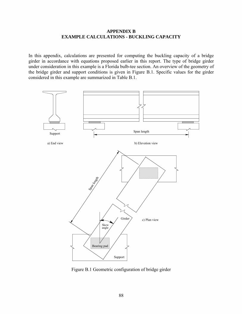
88
APPENDIX B EXAMPLE CALCULATIONS - BUCKLING CAPACITY
In this appendix, calculations are presented for computing the buckling capacity of a bridge girder in accordance with equations proposed earlier in this report. The type of bridge girder under consideration in this example is a Florida bulb-tee section. An overview of the geometry of the bridge girder and support conditions is given in Figure B.1. Specific values for the girder considered in this example are summarized in Table B.1.
Skewangle
Bearing pad
Span length
Support
Girder
Span
leng
th
Support
a) End view b) Elevation view
c) Plan view
Figure B.1 Geometric configuration of bridge girder
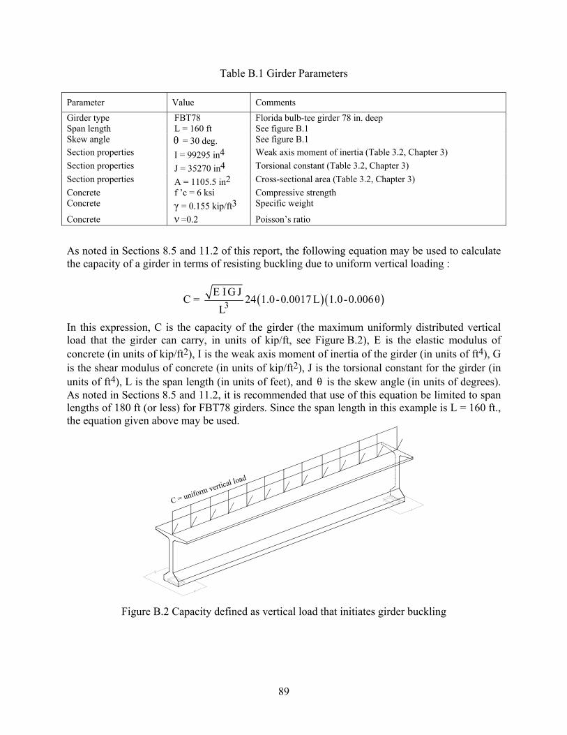
89
Table B.1 Girder Parameters
Parameter Value Comments
Girder type FBT78 Florida bulb-tee girder 78 in. deep Span length L = 160 ft See figure B.1 Skew angle θ = 30 deg. See figure B.1 Section properties I = 99295 in4 Weak axis moment of inertia (Table 3.2, Chapter 3) Section properties J = 35270 in4 Torsional constant (Table 3.2, Chapter 3) Section properties A = 1105.5 in2 Cross-sectional area (Table 3.2, Chapter 3) Concrete f ’c = 6 ksi Compressive strength Concrete γ = 0.155 kip/ft3 Specific weight
Concrete ν =0.2 Poisson’s ratio
As noted in Sections 8.5 and 11.2 of this report, the following equation may be used to calculate the capacity of a girder in terms of resisting buckling due to uniform vertical loading :
( ) ( )3E I G J
C = 24 1.0-0.0017 L 1.0-0.006θL
In this expression, C is the capacity of the girder (the maximum uniformly distributed vertical load that the girder can carry, in units of kip/ft, see Figure B.2), E is the elastic modulus of concrete (in units of kip/ft2), I is the weak axis moment of inertia of the girder (in units of ft4), G is the shear modulus of concrete (in units of kip/ft2), J is the torsional constant for the girder (in units of ft4), L is the span length (in units of feet), and θ is the skew angle (in units of degrees). As noted in Sections 8.5 and 11.2, it is recommended that use of this equation be limited to span lengths of 180 ft (or less) for FBT78 girders. Since the span length in this example is L = 160 ft., the equation given above may be used.
C = uniform vertical load
Figure B.2 Capacity defined as vertical load that initiates girder buckling
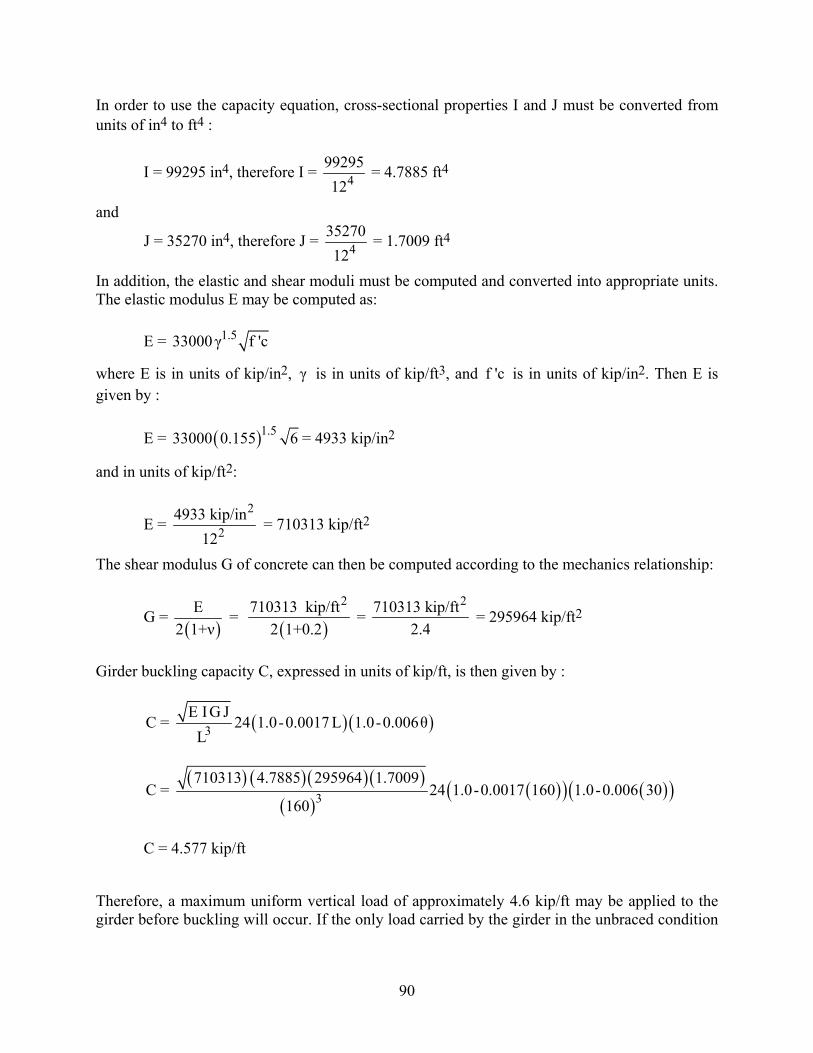
90
In order to use the capacity equation, cross-sectional properties I and J must be converted from units of in4 to ft4 :
I = 99295 in4, therefore I = 49929512
= 4.7885 ft4
and
J = 35270 in4, therefore J = 43527012
= 1.7009 ft4
In addition, the elastic and shear moduli must be computed and converted into appropriate units. The elastic modulus E may be computed as:
E = 1.533000 γ f 'c
where E is in units of kip/in2, γ is in units of kip/ft3, and f 'c is in units of kip/in2. Then E is given by :
E = ( )1.533000 0.155 6 = 4933 kip/in2
and in units of kip/ft2:
E = 2
24933 kip/in
12 = 710313 kip/ft2
The shear modulus G of concrete can then be computed according to the mechanics relationship:
G = ( )
E2 1+ν
= ( )
2710313 kip/ft2 1+0.2
= 2710313 kip/ft
2.4 = 295964 kip/ft2
Girder buckling capacity C, expressed in units of kip/ft, is then given by :
( ) ( )3E IG J
C = 24 1.0-0.0017 L 1.0-0.006θL
( ) ( ) ( ) ( )
( )( )( ) ( )( )3
710313 4.7885 295964 1.7009C = 24 1.0-0.0017 160 1.0-0.006 30
160
C = 4.577 kip/ft
Therefore, a maximum uniform vertical load of approximately 4.6 kip/ft may be applied to the girder before buckling will occur. If the only load carried by the girder in the unbraced condition
91
is its own self-weight, then the factor of safety against buckling may be computed as follows. The cross-sectional area is given by:
A = 1105.5 in2, therefore A = 21105.5
12 = 7.677 ft2
Volume per unit length of girder is : V = A (1 ft.) / ft = (7.677 ft2)(1 ft.) / ft = 7.677 ft3 / ft
The structural demand, D, on the girder is given by the self-weight of the girder per unit length, expressed in units of kip/ft. The weight of a 1 ft. length of girder is:
W = γV = ( ) ( )0.155 7.677 = 1.190 kip/ft ≈ 1.2 kip/ft
The factor of safety against buckling is then equal to the capacity to demand (C/D) ratio : FS = C/D = (4.6 kip/ft) / (1.2 kip/ft) = 3.8
In Section 11.2, it is recommended that the factor of safety not be less than 3.0 for buckling, therefore in this example, the girder has adequate capacity against buckling. As noted in Sections 8.5 and 11.2, capacities computed using the equation :
( ) ( )3E IG J
C = 24 1.0-0.0017 L 1.0-0.006θL
are based on limit states related to lateral buckling (girder stability) and tensile flange stresses (cracking). Additional section capacity calculations based on alternative failures modes (e.g., compression failure in the flange, etc.) must also be conducted. Such calculations are not presented here because specific quantities and locations of prestressing and/or mild reinforcing steel have not been included in the example.
It must also be noted that the detrimental effects of horizontal wind loading are not included in the buckling capacity calculations presented in this example. The presence of horizontal wind pressure on a girder will reduce the magnitude of vertical gravity loading required to initiate buckling and instability. Hence, calculations in addition to those shown here must be performed in order to assess girder capacity under conditions of combined horizontal (wind) and vertical (gravity) loading.