lars/lasso - Department of Statistics and Data Science · I nd my plots, which are slightly di erent from those produced by the lars library, ... The LARS/lasso algorithm recursively

lars/lasso 1

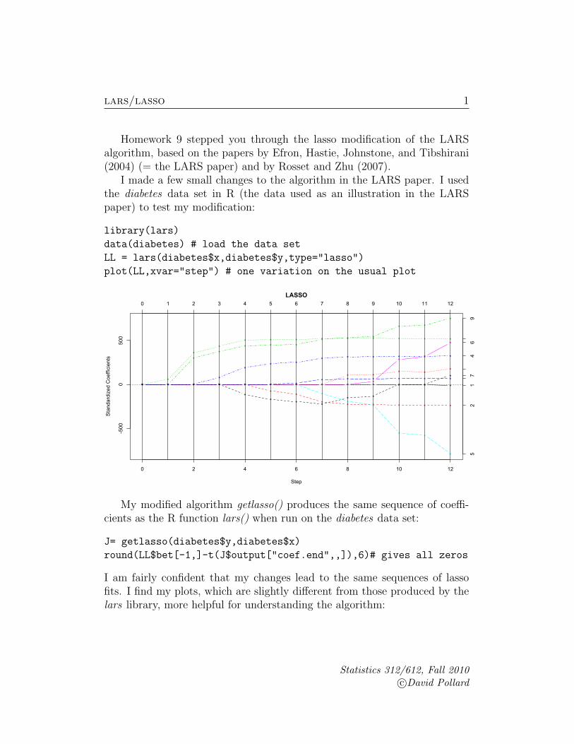
Homework 9 stepped you through the lasso modification of the LARSalgorithm, based on the papers by Efron, Hastie, Johnstone, and Tibshirani(2004) (= the LARS paper) and by Rosset and Zhu (2007).

I made a few small changes to the algorithm in the LARS paper. I usedthe diabetes data set in R (the data used as an illustration in the LARSpaper) to test my modification:

library(lars)

data(diabetes) # load the data set

LL = lars(diabetes$x,diabetes$y,type="lasso")

plot(LL,xvar="step") # one variation on the usual plot

* * * * * * * * * * * * *

0 2 4 6 8 10 12

-500

0500

Step

Sta

ndar

dize

d C

oeffi

cien

ts

* * * * ** *

* * * * * *

**

**

* * * * * * * * *

* * **

** *

* * * * * *

* * * * * * *

**

*

* *

*

* * * * * * * * * *

* *

*

* * * *

** * *

* *

* *

*

* * * * * * * *

* * * * *

* *

**

* * ** * *

* **

* * * * * * ** * * * * *

LASSO

52

17

46

9

0 1 2 3 4 5 6 7 8 9 10 11 12

My modified algorithm getlasso() produces the same sequence of coeffi-cients as the R function lars() when run on the diabetes data set:

J= getlasso(diabetes$y,diabetes$x)

round(LL$bet[-1,]-t(J$output["coef.end",,]),6)# gives all zeros

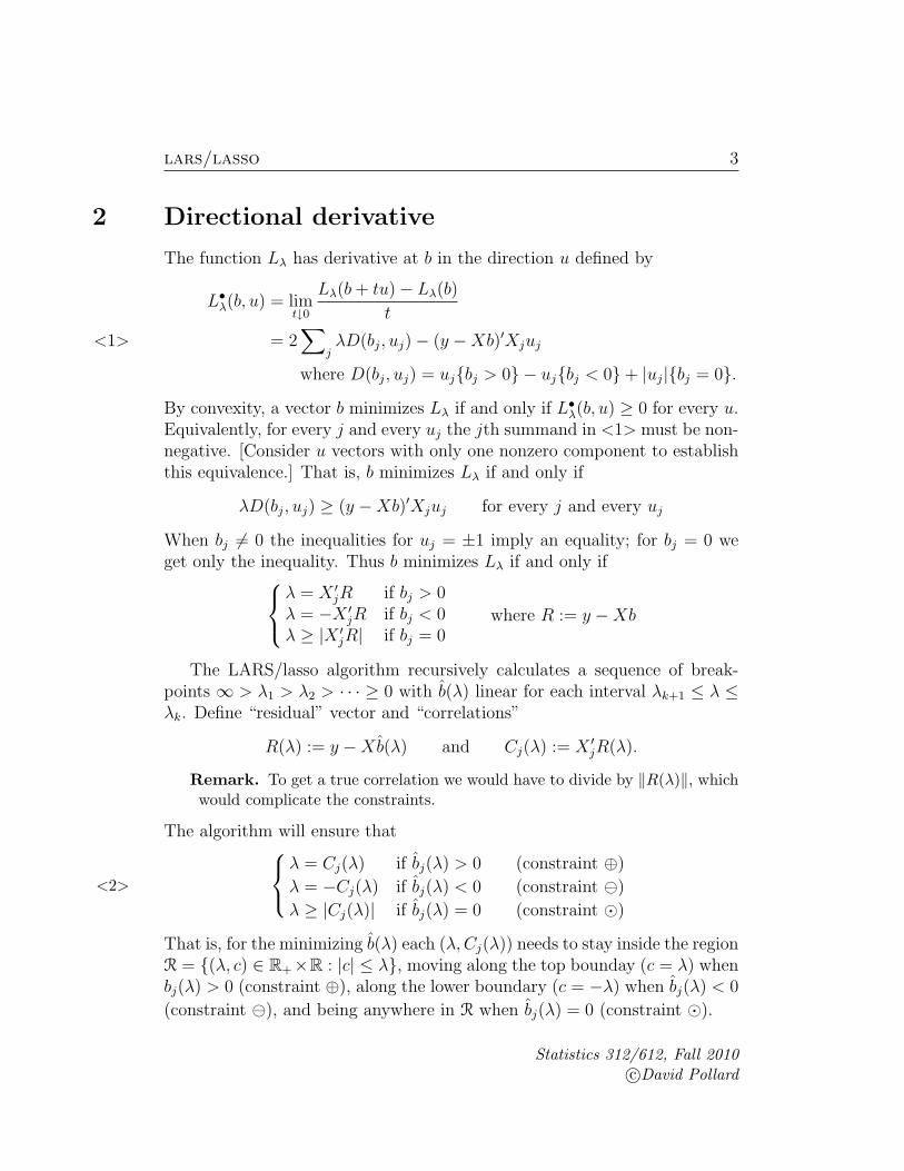
I am fairly confident that my changes lead to the same sequences of lassofits. I find my plots, which are slightly different from those produced by thelars library, more helpful for understanding the algorithm:

Statistics 312/612, Fall 2010c©David Pollard

lars/lasso 2

show2(J) # my plot

0 949.4889.3452.9316.1130.1

0

-949.4

949.4

Cj's

age, tc, ldl

sex

bmi, ltg

map, tch, glu

hdl

0

-792.2

751.3bj's

age, glu

sex

bmi, ldlmap

tc

hdl, tch

ltg

Modified lasso algorithm for diabetes data

[For higher resolution, see the pdf files attached to this handout.]

1 The Lasso problem

The problem is: given an n×1 vector y and an n×p matrix X, find the b(λ)that minimizes

Lλ(b) = ‖y −Xb‖2 + 2λ∑|bj|

for each λ ≥ 0. [The extra factor of 2 eliminates many factors of 2 in whatfollows.] The columns of X will be assumed to be standardized to have zeromeans and ‖Xj‖ = 1. I also seem to need linear independence of varioussubsets of columns of X, which would be awkward if p were larger than n.

Remark. I thought the vector y was also supposed to have a zero mean. Thatis not the case for the diabetes data set in R. It does not seem to be neededfor the algorithm to work.

I will consider only the “one at a time”case (page 417 of the LARS paper),for which the “active set” of predictors Xj changes only by either additionor deletion of a single predictor.


lars/lasso 3

2 Directional derivative

The function Lλ has derivative at b in the direction u defined by

L•λ(b, u) = limt↓0

Lλ(b+ tu)− Lλ(b)t

= 2∑

jλD(bj, uj)− (y −Xb)′Xjuj<1>

where D(bj, uj) = uj{bj > 0} − uj{bj < 0}+ |uj|{bj = 0}.

By convexity, a vector b minimizes Lλ if and only if L•λ(b, u) ≥ 0 for every u.Equivalently, for every j and every uj the jth summand in <1> must be non-negative. [Consider u vectors with only one nonzero component to establishthis equivalence.] That is, b minimizes Lλ if and only if

λD(bj, uj) ≥ (y −Xb)′Xjuj for every j and every uj

When bj 6= 0 the inequalities for uj = ±1 imply an equality; for bj = 0 weget only the inequality. Thus b minimizes Lλ if and only if

λ = X ′jR if bj > 0λ = −X ′jR if bj < 0λ ≥ |X ′jR| if bj = 0

where R := y −Xb

The LARS/lasso algorithm recursively calculates a sequence of break-points ∞ > λ1 > λ2 > · · · ≥ 0 with b(λ) linear for each interval λk+1 ≤ λ ≤λk. Define “residual” vector and “correlations”

R(λ) := y −Xb(λ) and Cj(λ) := X ′jR(λ).

Remark. To get a true correlation we would have to divide by ‖R(λ)‖, whichwould complicate the constraints.

The algorithm will ensure thatλ = Cj(λ) if bj(λ) > 0 (constraint ⊕)

λ = −Cj(λ) if bj(λ) < 0 (constraint )

λ ≥ |Cj(λ)| if bj(λ) = 0 (constraint �)

<2>

That is, for the minimizing b(λ) each (λ,Cj(λ)) needs to stay inside the regionR = {(λ, c) ∈ R+×R : |c| ≤ λ}, moving along the top bounday (c = λ) whenbj(λ) > 0 (constraint ⊕), along the lower boundary (c = −λ) when bj(λ) < 0

(constraint ), and being anywhere in R when bj(λ) = 0 (constraint �).


lars/lasso 4

3 The algorithm

The solution b(λ) is continuous in λ and linear on intervals defined by changepoints ∞ = λ0 > λ1 > λ2 > · · · > 0. The construction proceeds in steps,starting with large λ and working towards λ = 0. The vector of fitted valuesf(λ) = Xb(λ) is also piecewise linear. Within each interval (λk+1, λk) onlythe “active subset” A = Ak = {j : bj(λ) 6= 0} of the coefficients changes; theinactive coefficients stay fixed at zero.

3.1 Some illuminating special cases

It helped me to work explicitly through the first few steps before thinkingabout the equations that define a general step in the algorithm.

Start with A0 = ∅ and b(λ) = 0 for λ ≥ λ1 := max |X ′jy|. Constraint �is satisfied on [λ1,∞).

Step 1.

Constraint � would be violated if we kept b(λ) equal to zero for λ < λ1,because we would have maxj |Cj(λ)| > λ. The b(λ) must move away fromzero as λ decreases below λ1.

We must have |Cj(λ1)| = λ1 for at least one j. For convenience of ex-position, suppose C1(λ1) = λ1 > |Cj(λ1)| for all j ≥ 2. The active set nowbecomes A = {1}.

For λ2 ≤ λ < λ1, with λ2 to be specified soon, keep bj(λ) = 0 for j ≥ 2but let

b1(λ) = 0 + v1(λ1 − λ)

for some constant v1. To maintain the equalities

λ = C1(λ) = X ′1(y −X1b1(λ))

= C1(λ1)−X ′1X1v1(λ1 − λ) = λ1 − v1(λ1 − λ)

we need v1 = 1. This choice also ensures that b1(λ) > 0 for a while, so that ⊕is the relevant constraint for b1.

For λ < λ1, with v1 = 1 we have R(λ) = y −X1(λ1 − λ) and

Cj(λ) = Cj(λ1)− aj(λ1 − λ) where aj := X ′jX1.

Notice that |aj| < 1 unless Xj = ±X1. Also, as long as maxj≥2 |Cj(λ)| ≤ λ

the other bj’s still satisfy constraint �.


lars/lasso 5

We need to end the first step at λ2, the largest λ less than λ1 for whichmaxj≥2 |Cj(λ)| = λ. Solve for Cj(λ) = ±λ for each fixed j ≥ 2:

λ = λ1 − (λ1 − λ) = Cj(λ1)− aj(λ1 − λ)

−λ = −λ1 + (λ1 − λ) = Cj(λ1)− aj(λ1 − λ)

if and only if

λ1 − λ = (λ1 − Cj(λ1)) /(1− aj)λ1 − λ = (λ1 + Cj(λ1)) /(1 + aj)

Both right-hand sides are strictly positive. Thus λ2 = λ1 −∆λ where

∆λ := minj≥2 min

(λ1 − Cj(λ1)

1− aj,λ1 + Cj(λ1)

1 + aj

)<3>

Second step.

We have C1(λ2) = λ2 = maxj≥2 |Cj(λ2)|, by construction. For convenienceof exposition, suppose |C2(λ2)| = λ2 > |Cj(λ2)| for all j ≥ 3. The active setnow becomes A = {1, 2}.

To emphasize a subtle point it helps to consider separately two cases.Write s2 for sign(C2(λ2)), so that C2(λ2) = s2λ2.

case s2 = +1:For λ3 ≤ λ < λ2 and a new v1 and v2 (Note the recycling of notation.), define

b1(λ) = b1(λ2) + (λ2 − λ)v1

b2(λ) = 0 + (λ2 − λ)v2

with all other bj’s still zero. Write Z for [X1, X2]. The new Cj’s become

Cj(λ) = X ′j

(y −X1b1(λ)−X2b2(λ)

)= Cj(λ2)− (λ2 − λ)X ′jZv where v′ = (v1, v2).

We keep C1(λ) = C2(λ) = λ if we choose v to make X ′1Zv = 1 = X ′2v. Thatis, we need

v = (Z ′Z)−11 with 1 = (1, 1)′.

Of course we must assume that X1 and X2 are linearly independent for Z ′Zto have an inverse.


lars/lasso 6

case s2 = −1:For λ3 ≤ λ < λ2 and a new v1 and v2, define

b1(λ) = b1(λ2) + (λ2 − λ)v1

b2(λ) = 0− (λ2 − λ)v2 (note the change of sign)

with all other bj’s still zero. Write Z for [X1,−X2]. The tricky business withthe signs ensures that

Xb(λ)−Xb(λ2) = X1(λ2 − λ)v1 −X2(λ2 − λ)v2 = (λ2 − λ)Zv.

The new Cj’s become

Cj(λ) = X ′j

(y −X1b1(λ)−X2b2(λ)

)= Cj(λ2)− (λ2 − λ)X ′jZv.

We keep C1(λ) = −C2(λ) = λ if we choose v to make X ′1Zv = 1 = −X ′2v.That is, again we need v = (Z ′Z)−11.

Remark. If we had assumed C1(λ1) = −λ1 thenX1 would be replaced by−X1

in the Z matrix, that is, Z = [s1X1, s2X2] with s1 = sign(C1(λ1)) and s2 =sign(C2(λ2)).

Because b1(λ2) > 0, the correlation C1(λ) stays on the correct boundaryfor the ⊕ constraint. If s2 = +1 we need v2 > 0 to keep b2(λ) > 0 andC2(λ) = λ, satisfying ⊕. If s2 = −1 we also need v2 > 0 to keep b2(λ) < 0and C2(λ) = −λ, satisfying . That is, in both cases we need v2 > 0.

Why do we get a strictly positive v2? Write ρ for s2X′2X1. As the Z ′Z

matrix is nonsingular we must have |ρ| < 1 so that

v =

(1 ρρ 1

)−1

1 = (1− ρ2)−1

(1 −ρ−ρ 1

)1

and v2 = v1 = (1− ρ)/(1− ρ2) > 0.If no further Cj(λ)’s were to hit the ±λ boundary, step 2 could continue

all the way to λ = 0. More typically, we would need to create a new activeset at the largest λ3 strictly smaller than λ2 for which maxj≥3 |Cj(λ)| = λ.

For the general step there is another possible event that would require achange to the active set: one of the bj(λ)’s in the active set might hit zero,threatening to change sign and leave the corresponding Cj(λ) on the wrongboundary.

I could pursue these special cases further, but it is better to start againfor the generic step in the algorithm.


lars/lasso 7

3.2 The general algorithm

Once again, start with A0 = ∅ and b(λ) = 0 for λ ≥ λ1 := max |X ′jy|.Constraint � is satisfied on [λ1,∞).

At each λk a new active set Ak is defined. During the kth step the param-eter λ decreases from λk to λk+1. For all j’s in the active set Ak, the coeffi-cients bj(λ) change linearly and the Cj(λ)’s move along one of the boundaries

of the feasible region: Cj(λ) = λ if bj(λ) > 0 and Cj(λ) = −λ if bj(λ) < 0.

For each inactive j the coefficient bj(λ) remains zero throughout [λk+1, λk].Step k ends when either an inactive Cj(λ) hits a ±λ boundary or if an

active bj(λ) becomes zero: λk+1 is defined as the largest λ less than λk forwhich either of these conditions holds:

(i) maxj /∈Ak|Cj(λ)| = λ. In that case add the new j ∈ Ack for which

|Cj(λk+1)| = λk+1 to the active set, then proceed to step k + 1.

(ii) bj(λ) = 0 for some j ∈ Ak. In that case, remove j from the active set,then proceed to step k + 1.

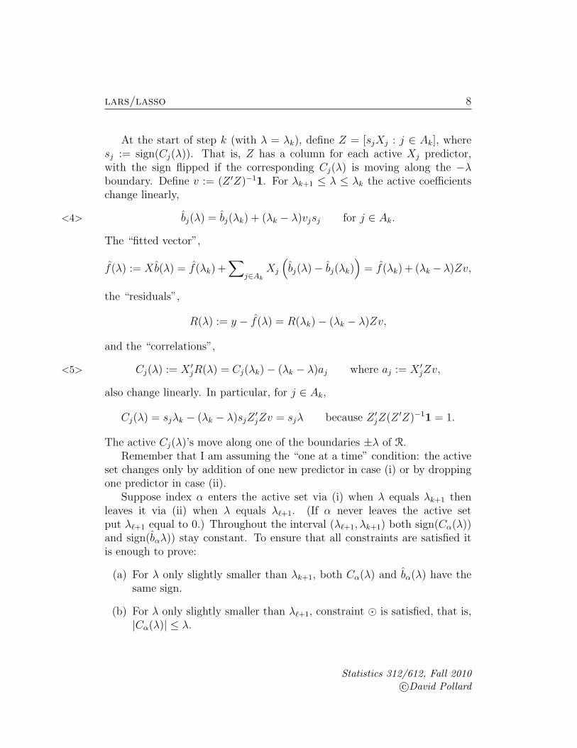
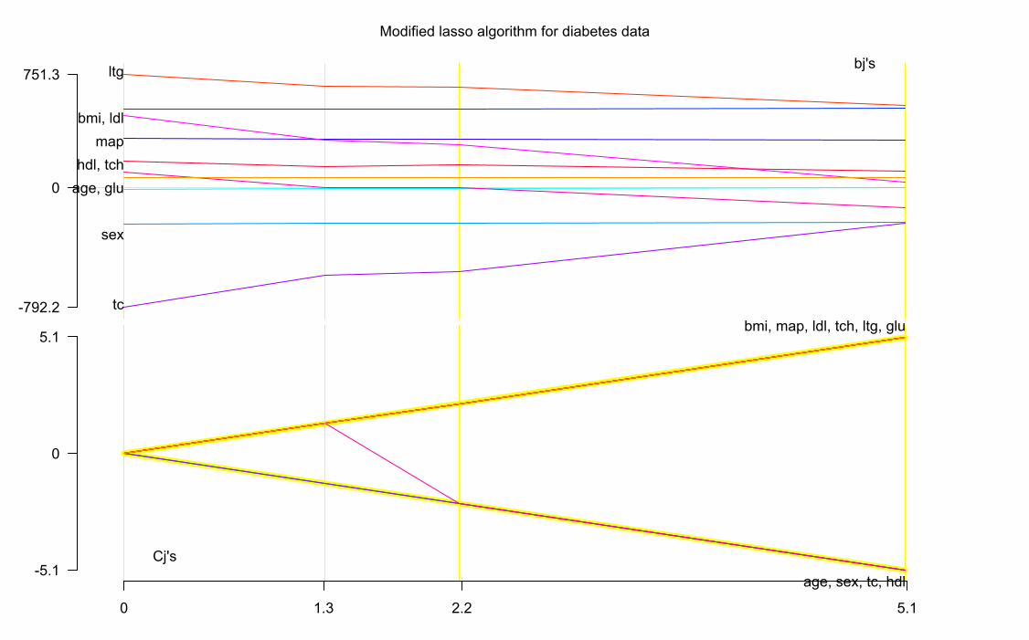
For the diabetes data, the alternative (ii) caused the behavior shown belowfor 1.3 ≤ λ ≤ 2.2.

0 5.12.21.3

0

-5.1

5.1

Cj's

age, sex, tc, hdl

bmi, map, ldl, tch, ltg, glu

0

-792.2

751.3bj's

age, glu

sex

bmi, ldlmap

tc

hdl, tch

ltg


I will show how the Cj(λ)’s and the bj(λ)’s can be chosen so that theconditions <2> are always satisfied.


lars/lasso 8

At the start of step k (with λ = λk), define Z = [sjXj : j ∈ Ak], wheresj := sign(Cj(λ)). That is, Z has a column for each active Xj predictor,with the sign flipped if the corresponding Cj(λ) is moving along the −λboundary. Define v := (Z ′Z)−11. For λk+1 ≤ λ ≤ λk the active coefficientschange linearly,

bj(λ) = bj(λk) + (λk − λ)vjsj for j ∈ Ak.<4>

The “fitted vector”,

f(λ) := Xb(λ) = f(λk) +∑

j∈Ak

Xj

(bj(λ)− bj(λk)

)= f(λk) + (λk − λ)Zv,

the “residuals”,

R(λ) := y − f(λ) = R(λk)− (λk − λ)Zv,

and the “correlations”,

Cj(λ) := X ′jR(λ) = Cj(λk)− (λk − λ)aj where aj := X ′jZv,<5>

also change linearly. In particular, for j ∈ Ak,

Cj(λ) = sjλk − (λk − λ)sjZ′jZv = sjλ because Z ′jZ(Z ′Z)−11 = 1.

The active Cj(λ)’s move along one of the boundaries ±λ of R.Remember that I am assuming the “one at a time” condition: the active

set changes only by addition of one new predictor in case (i) or by droppingone predictor in case (ii).

Suppose index α enters the active set via (i) when λ equals λk+1 thenleaves it via (ii) when λ equals λ`+1. (If α never leaves the active setput λ`+1 equal to 0.) Throughout the interval (λ`+1, λk+1) both sign(Cα(λ))and sign(bαλ)) stay constant. To ensure that all constraints are satisfied itis enough to prove:

(a) For λ only slightly smaller than λk+1, both Cα(λ) and bα(λ) have thesame sign.

(b) For λ only slightly smaller than λ`+1, constraint � is satisfied, that is,|Cα(λ)| ≤ λ.


lars/lasso 9

The analyses are similar for the two cases. They both depend on a neatformula for inversion of symmetric block matrices. Suppose A is an m ×mnonsingular, symmetric matrix and d is an m × 1 vector for which κ :=1− d′A−1d 6= 0. Then(

A dd′ 1

)−1

=

(A−1 + ww′/κ −w/κ

−w′/κ 1/κ

)where w := A−1d .<6>

This formula captures the ideas involved in Lemma 4 of the LARS paper.For simplicity of notation, I will act in both cases (a) and (b) as if the α

is larger than all the other j’s that were in the active set. (More formally, Icould replace X in what follows by XE for a suitable permutation matrix E.)The old and new Z matrices then have the block form shown in <6>.

Case (a): α enters the active set at λk+1

As for the analysis that led to the expression in <3>, the solutions for λ =|Cj(λ)| with j ∈ Ack are given by

(λk − λ)(1− aj) = λk − Cj(λk) to get λ = Cj(λ)

(λk − λ)(1 + aj) = λk + Cj(λk) to get − λ = Cj(λ)

Index α is brought into the active set because |Cα(λk+1)| = λk+1. Thus

(λk − λ′k+1)(1− sαaα) = λk − sαCα(λk) where sα := sign(Cα(λ′k+1)).

Note that |Cα(λk)| < λk because α was not active during step k. It followsthat the right-hand side of the last equality is strictly positive, which implies

1− sαaα > 0.<7>

Throughout a small neighborhood of λk+1 the sign sα of Cα(λ) stays thesame. Continue to write Z for the active matrix [sjXj; j ∈ Ak] for λ slightlylarger than λk+1 and denote by

Z = [sjXj; j ∈ Ak+1] = [Z, sαXα]

the new active matrix for λ slightly small than λk+1. Then

Z ′Z =

(Z ′Z d

d′ 1

)where d := sαZ

′Xα .


lars/lasso 10

Notice that

1− κ = d′A−1d = X ′αZ(Z ′Z)−1Z ′Xα = ‖HXα‖2 ,

where H = Z(Z ′Z)−1Z ′ is the matrix that projects vectors orthogonallyonto span(Z). If Xα /∈ span(Z) then ‖HXα‖ < ‖Xα‖ = 1 so that κ > 0.From <6>,

(Z ′Z)−1 =

((Z ′Z)−1 + ww′/κ −w/κ

−w′/κ 1/κ

)where w := sα(Z ′Z)−1Z ′Xα .<8>

The αth coordinate of the new v = (Z ′Z)−11 equals vα = κ−1 (1− w′1),which is strictly positive because

1− w′1 = 1− sαX ′αZ(Z ′Z)−11

= 1− sαX ′αZv= 1− sαaα by <5>

> 0 by <7>.

By <4>, the new bα(λ) = (λk+1 − λ)vαsα has the same sign, sα, as Cα(λ).

Case (b): α leaves the active set at λ = λ`+1

The roles of Z = [sjXj : 1 ≤ j < α] and Z = [Z, sαXα] are now re-

versed. For λ slightly larger than λ`+1 the active matrix is Z, and bothCα(λ) and bα(λ) have sign sα.

Index α leaves the active set because bα(λ`+1) = 0. Thus

0 = bα(λ`) + (λ` − λ`+1)vαsα

where sα := sign(Cα(λ`)) and v = (Z ′Z)−11. The active bα(λ`) also hadsign sα. Consequently, we must have

vα < 0.<9>

For λ slightly smaller than λ`+1 the active matrix is Z, and, by <5>,

sαCα(λ) = λ`+1 − (λ`+1 − λ)sαaα where aα := X ′αZv

= λ+ (λ`+1 − λ)(1− sαaα)


lars/lasso 11

We also know that

0 > κvα = 1− w′1 = 1− sαaα.

Thus sαCα(λ) < λ, and hence |Cα(λ)| < λ, for λ slightly less than λ`+1. Thenew Cα(λ) satisfies constraint ⊕ as it heads off towards the other boundary.

Remark. Clearly there is some sort of duality accounting for the similaritiesin the arguments for cases (a) and (b), with <6> as the shared mechanism. Ifwe think of λ as time, case (b) is a time reversal of case (a). For case (a) thedefining condition (Cα hits the boundary) at λk+1 gives 1− sαvα > 0, whichimplies vα > 0. For case (b), the defining condition (bα hits zero) at λ`+1

gives va < 0, which implies 1− sαaα < 0.Is there some clever way to handle both cases by a duality argument?

Maybe I should read more of the LARS paper.

4 My getlasso() function

I wrote the R code in the file lasso.R to help me understand the algorithmdescribed in the LARS paper. The function is not particularly elegant orefficient. I wrote in a way that made it easy to examine the output fromeach step. If verbose=T, lots of messages get written to the console and thefunction pauses after each step. I also used some calls to browser() whiletracking down some annoying bugs related to case (b).

d.p. 1 December 2010

References

Efron, B., T. Hastie, I. Johnstone, and R. Tibshirani (2004). Least angleregression. The Annals of Statistics 32 (2), pp. 407–451.

Rosset, S. and J. Zhu (2007). Piecewise linear regularized solution paths.Annals of Statistics 35 (3), 1012–1030.


0 949.4889.3452.9316.1130.1

0

-949.4

949.4

Cj's

age, tc, ldl

sex

bmi, ltg

map, tch, glu

hdl

0

-792.2

751.3bj's

age, glu

sex

bmi, ldlmap

tc

hdl, tch

ltg


949.4889.3452.9

0

-949.4

949.4

Cj's

age, tc, ldl

sex

bmi, ltg

map, tch, glu

hdl

0

361.9bj's

age, sex, map, tc, ldl, hdl, tch, glu

bmi

ltg


949.4889.3452.9316.1

0

-949.4

949.4

Cj's

age, tc, ldl

sex

bmi, ltg

map, tch, glu

hdl

0

434.8bj's

age, sex, tc, ldl, hdl, tch, glu

bmi

map

ltg


949.4889.3452.9316.1130.1

0

-949.4

949.4

Cj's

age, tc, ldl

sex

bmi, ltg

map, tch, glu

hdl

0

-114.1

505.7bj's

age, sex, tc, ldl, tch, glu

bmi

map

hdl

ltg


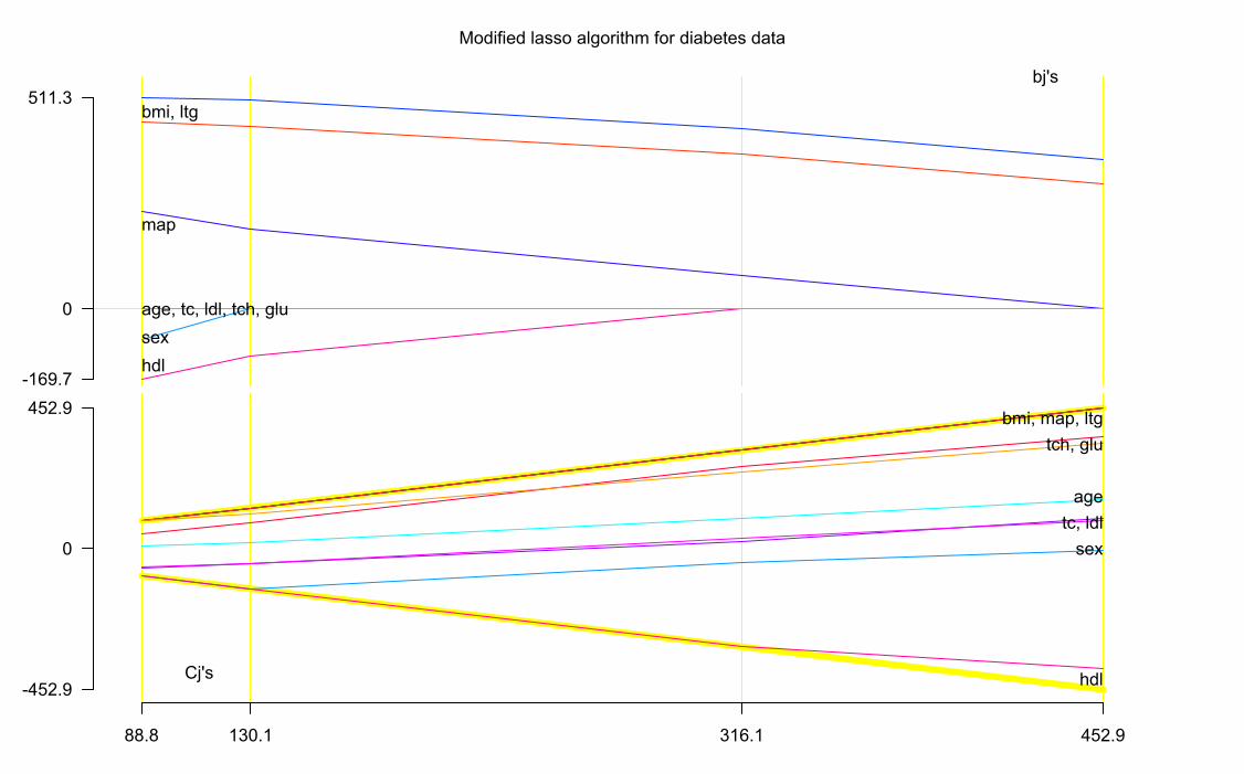
452.9316.1130.188.8

0

-452.9

452.9

Cj's

age

sex

bmi, map, ltg

tc, ldl

hdl

tch, glu

0

-169.7

511.3bj's

age, tc, ldl, tch, glusex

bmi, ltg

map

hdl


0 205.52.2

0

-20

20

Cj's

age

sex, tc, hdl

bmi, map, tch, ltg, glu

ldl

0

-792.2

751.3bj's

age, glu

sex

bmi, ldlmap

tc

hdl, tch

ltg


0 5.12.21.3

0

-5.1

5.1

Cj's

age, sex, tc, hdl

bmi, map, ldl, tch, ltg, glu

0

-792.2

751.3bj's

age, glu

sex

bmi, ldlmap

tc

hdl, tch

ltg


Documents

lars/lasso - Department of Statistics and Data Science · I nd my plots, which are slightly di erent from those produced by the lars library, ... The LARS/lasso algorithm recursively