Embed Size (px)
Citation preview
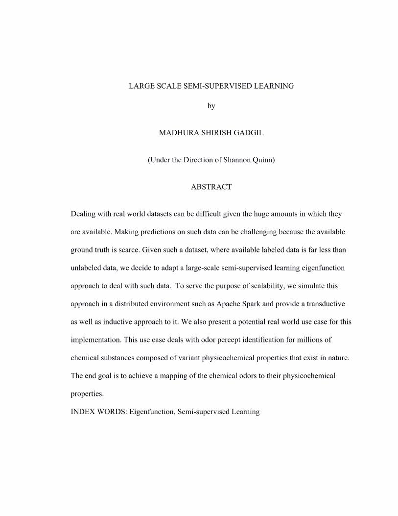
LARGE SCALE SEMI-SUPERVISED LEARNING
by
MADHURA SHIRISH GADGIL
(Under the Direction of Shannon Quinn)
ABSTRACT
Dealing with real world datasets can be difficult given the huge amounts in which they
are available. Making predictions on such data can be challenging because the available
ground truth is scarce. Given such a dataset, where available labeled data is far less than
unlabeled data, we decide to adapt a large-scale semi-supervised learning eigenfunction
approach to deal with such data. To serve the purpose of scalability, we simulate this
approach in a distributed environment such as Apache Spark and provide a transductive
as well as inductive approach to it. We also present a potential real world use case for this
implementation. This use case deals with odor percept identification for millions of
chemical substances composed of variant physicochemical properties that exist in nature.
The end goal is to achieve a mapping of the chemical odors to their physicochemical
properties.
INDEX WORDS: Eigenfunction, Semi-supervised Learning

LARGE SCALE SEMI-SUPERVISED LEARNING
by
MADHURA SHIRISH GADGIL
B.E., UNIVERSITY OF PUNE, INDIA, 2012
A Thesis Submitted to the Graduate Faculty of The University of Georgia in Partial
Fulfillment of the Requirements for the Degree
MASTER OF SCIENCE
ATHENS, GEORGIA 2016

© 2016
Madhura Shirish Gadgil
All Rights Reserved

LARGE SCALE SEMI-SUPERVISED LEARNING
by
MADHURA SHIRISH GADGIL
Major Professor: Shannon Quinn Committee: Lakshmish Ramaswamy
Khaled Rasheed
Electronic Version Approved:
Suzanne Barbour Dean of the Graduate School The University of Georgia December 2016

iv
DEDICATION
To my parents, family, friends, colleagues and my advisor for their support, guidance and
encouragement.

v
ACKNOWLEDGEMENTS
I would like to thank Dr. Shannon Quinn for his immense guidance throughout this
project and also during my academic career here at UGA. I thank him for introducing me
to this ocean of Data Science and Machine Learning. I would also like to thank my
colleagues and friends for their support and guidance during my graduate academic
career.
vi
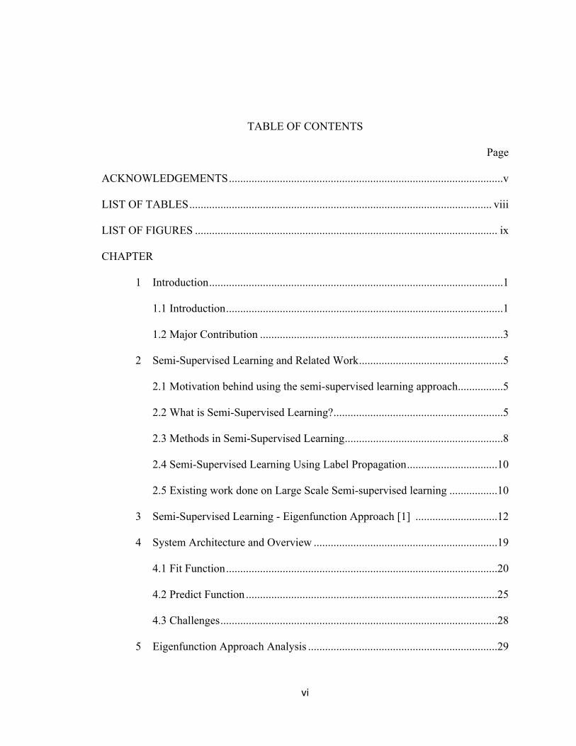
TABLE OF CONTENTS
Page
ACKNOWLEDGEMENTS .................................................................................................v
LIST OF TABLES ........................................................................................................... viii
LIST OF FIGURES ........................................................................................................... ix
CHAPTER
1 Introduction ........................................................................................................1
1.1 Introduction ..................................................................................................1
1.2 Major Contribution ......................................................................................3
2 Semi-Supervised Learning and Related Work ...................................................5
2.1 Motivation behind using the semi-supervised learning approach ................5
2.2 What is Semi-Supervised Learning? ............................................................5
2.3 Methods in Semi-Supervised Learning ........................................................8
2.4 Semi-Supervised Learning Using Label Propagation ................................10
2.5 Existing work done on Large Scale Semi-supervised learning .................10
3 Semi-Supervised Learning - Eigenfunction Approach [1] .............................12
4 System Architecture and Overview .................................................................19
4.1 Fit Function ................................................................................................20
4.2 Predict Function .........................................................................................25
4.3 Challenges ..................................................................................................28
5 Eigenfunction Approach Analysis ...................................................................29
vii
5.1 Data Densities ............................................................................................29
5.2 Data points against Approximate Eigenvectors .........................................30
5.3 Data points against smoothness functions .................................................32
6 Results .............................................................................................................33
6.1 Results on Small dataset ............................................................................33
6.2 Results on Bigger Dataset .........................................................................35
6.3 Standalone Performance Vs Large-Scale Performance .............................38
6.4 Parameters vs. Accuracy ............................................................................41
6.5 Nodes Vs Time ..........................................................................................43
7 Potential Use Case: Computational Olfaction .................................................45
7.1 Introduction ...............................................................................................45
7.2 Computational Olfaction – Background ...................................................47
7.2.1 “Odor quality: semantically generated multidimensional profiles are
stable”, [5] ..................................................................................................47
7.2.2 “In search of the structure of human olfactory space”, [6] ..............47
7.2.3 “Categorical Dimensions of Human Odor Descriptor
Space Revealed by Non- Negative Matrix Factorization”,[7] ...................48
7.3 Challenges ..................................................................................................51
8 Conclusion ......................................................................................................52
REFERENCES ..................................................................................................................54

viii
LIST OF TABLES
Page
Table 1: Standalone Performance Vs Large-Scale Performance for Precision .................38
Table 2: Standalone Performance Vs Large-Scale Performance for recall .......................39
Table 3: Standalone Performance Vs Large-Scale Performance for F1-Measure .............40
Table 4: Scalability for variant number of executors for fit function. (Time in seconds) 43
Table 5: Scalability for variant number of executors for predict function. (Time in
seconds) .................................................................................................................43
ix
LIST OF FIGURES
Figure 1: Far left: Original 2D toy data. Next three (left to right) are the first 3
eigenvectors, their values overlaid on the data. Next is the corresponding
density plots of the data. Finally, the numerical eigenfunctions of the data ..........15
Figure 2: Eigenfunction algorithm flow at a high level .....................................................16
Figure 3: Comparison of Eigenfunction approach and Nystrom Method. .........................17
Figure 4: Comparison of Eigenfunction approach on the tiny images dataset ..................18
Figure 5: Flow Process of the fit function .........................................................................21
Figure 6: Pseudo code for the fit function .........................................................................22
Figure 7: Clustering suggested by smoothness functions for 1000 data points with
binomial Clustering. ...............................................................................................24
Figure 8: Flow process for predict functions .....................................................................26
Figure 9: Pseudocode for Predict functions… ...................................................................27
Figure 10: Toy data blobs and the plot of their 2D densities using 2D histograms ...........29
Figure 11: Toy dataset (above) and below is its plot against first Eigenvector for the data.
Zeroth eigenvector will always be flat ...................................................................31
Figure 12: 2D densities of the corresponding toy dataset in the figure above versus its
corresponding smoothness function values ...........................................................32
Figure 13: Transductive Learning. Train data ground truth ..............................................33
x
Figure 14: Inductive learning. Test data ground truth .......................................................34
Figure 15: Transductive learning. Train data predicted labels ..........................................34
Figure 16: Inductive learning. Test data predicted labels ..................................................35
Figure 17: Training dataset with original clustering for first two dimensions. ................36
Figure 18: Labels propagated across the entire dataset with just 10 originally labeled
points available. One label available for each class. .............................................36
Figure 19: Test data set original clustering for first two dimensions. ..............................37
Figure 20: Label propagation after 1D interpolation of data using the learned model
parameters during the training phase. This depicts the Inductive Learning. ........37
Figure 21: Precision comparison for standalone and largescale ........................................39
Figure 22: Recall comparison for standalone and largescale .............................................40
Figure 23: F1-Measure comparison for standalone and largescale ...................................41
Figure 24: Effect of k and gamma values on Accuracy for different values of number of
histogram bins. Accuracy is measured with F1-Measure. As number of bins
increase, accuracy improves. The yellow region depicts the parameter
combinations (k, bins, and gamma) where the accuracy is high. ..........................42
Figure 25: Scalability in seconds for variant data sizes against variant executors ............44
Figure 26: Scalability in seconds for variant data sizes against variant executors ............44
Figure 27: 10 largest-valued descriptors for each of the 10 basis vectors obtained from
non-negative matrix factorization [7] ....................................................................49
Figure 28: 2D embedding of the odor perceptual space [7] ...............................................50

1
CHAPTER 1
INTRODUCTION
This chapter gives an introduction to the significance of semi-supervised learning and its
potential applications. It discusses some of the different methods of semi-supervised
learning.
1.1 Introduction
It is difficult to make predictions from real world datasets because of their large size and
unstructured formats. A good example can be images from surveillance cameras. If
predictions are to be made to detect objects in images, we need some ground truth to base
our predictions on. But if these images are available in huge numbers, it is practically
impossible to prepare ground truth by manually labeling more than a small fraction of the
images. To make this problem somewhat more feasible, we can attempt to combine the
small fraction of labeled data simultaneously with the unlabeled data in our model. In
such a situation, where labeled data is orders of magnitude smaller than unlabeled data, a
semi-supervised solution would work well.
Semi-supervised learning has two approaches, transductive and inductive learning.
In transductive learning, the whole dataset is used to build and train the model and
predictions are made on all of the training data.

2
Inductive learning does not require the unseen data to be passed through the training
phase again. Using the already trained model, predictions are made on unobserved data.
Our work is inspired by “Semi-supervised Learning in Gigantic Image Collections”, a
2009 paper by Fergus et al. The paper introduces an approach that is memory efficient for
large scale processing. The approach is dominated by approximations to efficiently build
a model for predictions. It uses semi-supervised learning approach by estimating a graph
Laplacian matrix for the given dataset, numerically approximates the eigenfunctions,
build interpolators and eventually derives the smoothness functions for the graph
Laplacian. These smoothness functions are responsible for classifying unlabeled data into
their corresponding classes depending on how smooth the function is with respect to the
data points if they were depicted on a manifold.
The above description was the transductive learning approach offered by Semi-
supervised learning. However, we anticipate the situation where we may wish to make
predictions on future unobserved data without recomputing the entire semi-supervised
model. Therefore, we have also implemented the inductive learning aspect of this
approach. For a new unseen data point we interpolate this point using the interpolators we
built during transductive learning and predict label for the interpolated values which are
nothing but the smoothness functions.
3
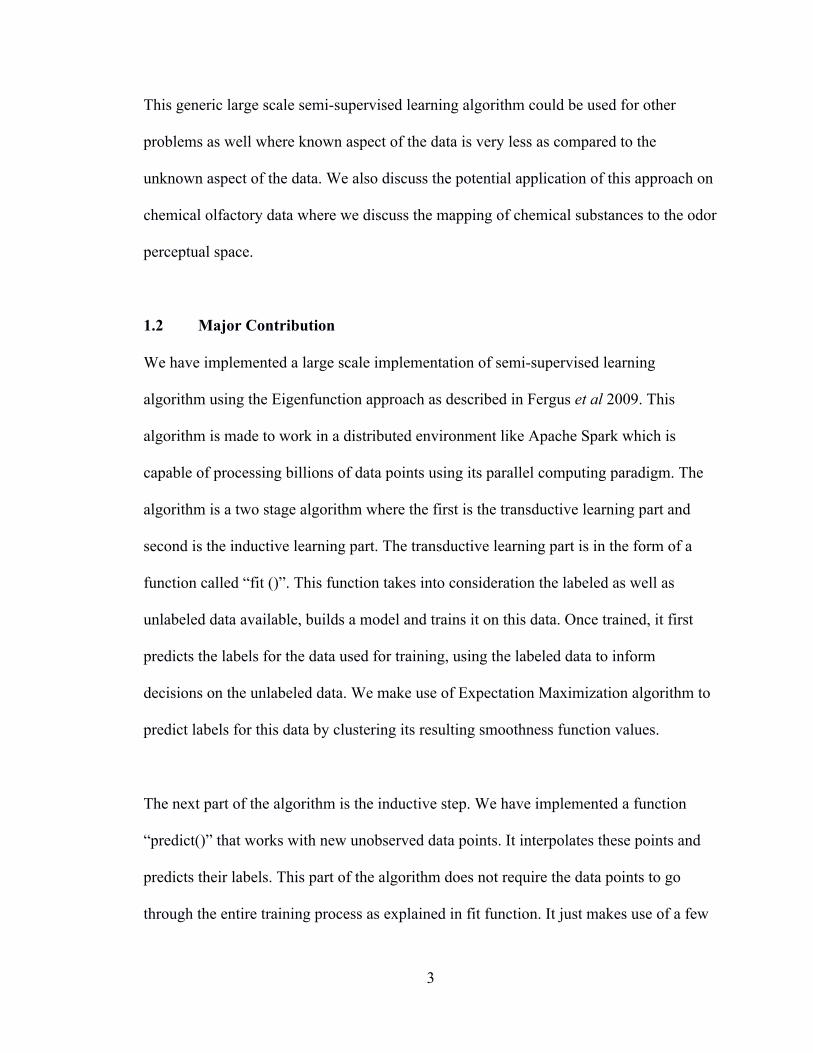
This generic large scale semi-supervised learning algorithm could be used for other
problems as well where known aspect of the data is very less as compared to the
unknown aspect of the data. We also discuss the potential application of this approach on
chemical olfactory data where we discuss the mapping of chemical substances to the odor
perceptual space.
1.2 Major Contribution
We have implemented a large scale implementation of semi-supervised learning
algorithm using the Eigenfunction approach as described in Fergus et al 2009. This
algorithm is made to work in a distributed environment like Apache Spark which is
capable of processing billions of data points using its parallel computing paradigm. The
algorithm is a two stage algorithm where the first is the transductive learning part and
second is the inductive learning part. The transductive learning part is in the form of a
function called “fit ()”. This function takes into consideration the labeled as well as
unlabeled data available, builds a model and trains it on this data. Once trained, it first
predicts the labels for the data used for training, using the labeled data to inform
decisions on the unlabeled data. We make use of Expectation Maximization algorithm to
predict labels for this data by clustering its resulting smoothness function values.
The next part of the algorithm is the inductive step. We have implemented a function
“predict()” that works with new unobserved data points. It interpolates these points and
predicts their labels. This part of the algorithm does not require the data points to go
through the entire training process as explained in fit function. It just makes use of a few
4
parameters that were learned from the fit function and derives smoothness functions for
the new data. Once we get those smoothness functions, we predict labels for them by
clustering it using the previously trained expectation maximization model.
We also discuss the potential application of this algorithm on chemical olfactory data and
present the computational olfaction as a case study.
The remainder of this document is structured as follows: CHAPTER 2 discusses the
concept of semi-supervised learning using label propagation. CHAPTER 3 talks about
available implementations of semi- supervised learning approaches and some background
on semi-supervised learning with graph based methods. CHAPTER 4 discusses the
algorithm in detail with the flowchart. CHAPTER 5 walks through the algorithm
discussing its nuances with relevant results.
CHAPTER 6 sums up our approach with a conclusion. CHAPTER 7 discusses the
potential use of this algorithm implementation in computational olfaction.
5
CHAPTER 2
SEMI-SUPERVISED LEARNING AND RELATED WORK
In this chapter, we discuss about Semi-supervised learning in general, work done on it
and then discuss our approach in depth.
2.1 Motivation behind using the semi-supervised learning (SSL) approach
With less ground truth, it is infeasible to train a purely supervised classifier to accurately
recognize the majority of possible data. Moreover, if we try to use unsupervised approach
then we lose out on the information that the labeled data provides. Thus, we can say that
semi-supervised learning works well on problems where there is a very small amount of
labeled data relative to the amount of unlabeled data. Such algorithms are scalable and
thus suitable for large datasets.
2.2 What is Semi-Supervised Learning?
Semi-supervised learning makes use of labeled as well as unlabeled data, and
incorporating both into the initial training step of the model. Imagine n data points with d
dimensions (n <<< d) which are independently and identically distributed. These n data
points can be divided into 2 parts such that
𝑋𝑙 ∶= 𝑥1, 𝑥2, … . , 𝑥𝑙 ; 𝑌𝑙 ∶= 𝑦1, 𝑦2,… . , 𝑦𝑙 … . . 𝑋𝑙, 𝑌𝑙𝑎𝑟𝑒𝑙𝑎𝑏𝑒𝑙𝑒𝑑𝑝𝑜𝑖𝑛𝑡𝑠
6
𝑋𝑢 ∶= 𝑥 𝑙 + 1 ,… . . , 𝑥 𝑙 + 𝑢 ……𝑎𝑟𝑒𝑢𝑛𝑙𝑎𝑏𝑒𝑙𝑒𝑑𝑝𝑜𝑖𝑛𝑡𝑠
The basic idea is, given a mapping of data points X to labels Y(f:X → Y), task is to
learn a better predictor f by implicitly ordering these predictor functions f ∈ Fwhich is
induced by the unlabeled data.
Ordinarily this ordering is interpreted as a prior over For as a regularizer. But if after
ordering, the target predictor function is found near the top of the ordering then you need
less labeled data to learn this predictor function [2].
Semi-supervised learning can be interpreted in two forms, transductive learning and
inductive learning. Given a set of labeled training set and an unlabeled test set, the idea of
transduction is to perform predictions only for the test points. Whereas, in case of
inductive learning the goal is to output a prediction function which is defined on the
entire space X [4], therefore capable of predicting novel, unobserved data without
rebuilding the entire model.
Semi-supervised learning was originally derived during estimation of the Fisher linear
discriminant rule using unlabeled data was considered (Hosmer, 1973; McLachlan, 1977;
O’Neill, 1978; McLachlan and Ganesalingam, 1982). Semi-supervised learning is
suitable where each class-conditional density is Gaussian with equal covariance matrix.
The likelihood of the model is then maximized using the labeled and unlabeled data with
the help of clustering algorithms like expectation-maximization (EM) algorithm [18].
One essential prerequisite for semi-supervised learning is that the distribution of
examples should be relevant to the classification problem especially with respect to the
7
unlabeled data. Mathematically speaking, the information given by distribution
𝑝(𝑥)should prove to be useful in the inference of 𝑝 𝑦 𝑥 .Otherwise, the semi-
supervised version would not prove to be more efficient over supervised version[4].
For semi-supervised learning to work efficiently, one of the following assumptions
should hold.
1. Smoothness Assumption: Points that are close to each other are more
likely to share the same label. “If two points 𝑥1, 𝑥2in a high-density region are
close, then so should be the corresponding outputs 𝑦1, 𝑦2.” Thus the goal is to find
smoothness function that fits the labeled data well. [4]
2. Cluster Assumption: If data clustering is known beforehand, then the
points in the same cluster are more likely to share a label. Simply put, “if points are
in the same cluster, they are likely to be of the same class”. Cluster assumption can
be thought of as a special case of smoothness assumption[4].
3. Manifold Assumption: “The high dimensional data lie roughly on a low
dimensional manifold”. This essentially means dimensionality reduction. The curse
of dimensionality has been a bottleneck for most learning methods. In generative
methods where data densities are used for estimation, data can grow exponentially
with a higher number of dimensions. Also, there are discriminative methods which
make use of pairwise distances. With high number of dimensions, these pairwise
distances become less expressive and more correlated. “If the data happen to lie on a
low-dimensional manifold, however, then the learning algorithm can essentially
8
operate in a space of corresponding dimension, thus avoiding the curse of
dimensionality.” [4].
Our approach is closely based on the Manifold Assumption since we will be dealing with
data densities and a lot of numerical approximations at lower dimensions.
2.3 Methods in Semi-Supervised Learning
There are two main things to be addressed by a semi-supervised learning method: what
implicit ordering of the functions is induced by the unlabeled data and how to find a
predictor function at the top of this ordering that fits the labeled data well [2]. In simple
words, we need to make a predictor that correctly identifies the data which we already
know and makes well defined predictions on data that is not known. We take a look at
different variations of semi-supervised learning in this section.
1. Generative Models: This method works on the assumption of joint probability
distribution given by Bayes’ rule, 𝑝 𝑥 𝑦, 𝜃 = 𝑝 𝑦 𝜃 ∗ 𝑝 𝑥 𝑦, 𝜃 ,where
𝑝 𝑦 𝜃 is the class prior distribution and 𝑝(𝑥|𝑦, 𝜃)is class conditional
distribution. θ denotes the parameters of joint probability. Each θ is associated
with a predictor function 𝑓Isuch𝑓I 𝑥 = argmaxO
𝑝 𝑦 𝑥, 𝜃 and the chosen 𝑓I is
the one that fits the labeled as well as unlabeled data well [2].
2. Low density Separation: Low density area is defined where there are fewer data
points. A classic example of this would be transductive SVM. TSVM labels the
unlabeled data that has maximal margin over all the data. TSVM then selects
function𝑓∗ 𝑥 = ℎ∗ 𝑥 + 𝑏 by minimizing the following:
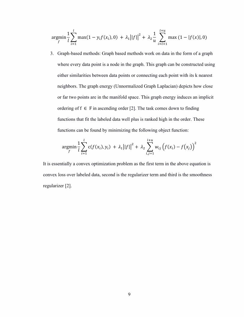
9
argminS
1𝑙 max 1 − 𝑦U𝑓 𝑥U , 0
W
UXY
+𝜆Y 𝑓 [ +𝜆[1𝑢 max(1 − 𝑓 𝑥 , 0)
W\]
UXW\Y
3. Graph-based methods: Graph based methods work on data in the form of a graph
where every data point is a node in the graph. This graph can be constructed using
either similarities between data points or connecting each point with its k nearest
neighbors. The graph energy (Unnormalized Graph Laplacian) depicts how close
or far two points are in the manifold space. This graph energy induces an implicit
ordering of f ∈ Fin ascending order [2]. The task comes down to finding
functions that fit the labeled data well plus is ranked high in the order. These
functions can be found by minimizing the following object function:
argminS
1𝑙 c 𝑓 𝑥U , 𝑦U
W
UXY
+𝜆Y 𝑓 [ +𝜆[ 𝑤U` 𝑓 𝑥U − 𝑓 𝑥[
W\]
U,`XY
It is essentially a convex optimization problem as the first term in the above equation is
convex loss over labeled data, second is the regularizer term and third is the smoothness
regularizer [2].

10
2.4 Semi-Supervised Learning Using Label Propagation
Label Propagation identifies community structures in the network. Because of this nature,
it is best suited for a graph setting [17]. All densely connected components in the network
carry same label. Every labeled node is initialized with a unique label which then
propagates through the network. The Label Propagation algorithm is similar to labeling
through k nearest neighbors. The graph based semi-supervised learning approach labels
the unlabeled points using label propagation; the smoothness regularizer term observed in
the previous section simulates the principle working of label propagation algorithm.
Label Propagation is a memory efficient algorithm hence it works well with semi-
supervised learning.
2.5 Existing work done on Large Scale Semi-supervised learning
This section talks about the existing work done on large scale semi-supervised learning
that find workaround for direct construction of the graph Laplacian.
1. Prototype Vector Machine for large Scale Semi-Supervised Learning [14]: This
method introduces a novel concept of prototypes vectors for better approximation
on graph-based regularizer and model representation. These vectors essentially
perform low rank approximation of the kernel matrix as well as help construct a
model that can allow minimum information loss compared with the complete
model. This low rank approximation prototypes help avoid the construction of
complete n x n kernel matrix. And the label reconstruction prototypes work only
on labels of k prototypes.

11
2. Large Graph Construction for Scalable Semi-Supervised Learning [15]: This
paper introduces a workaround for the construction of the graph Laplacian but
using anchor points that will cover the cloud of all points sufficiently. This paper
tries to construct the Laplacian using the anchor points and adjacency matrix in
combination. This approach constructs large sparse graphs over all the data.
12
CHAPTER 3
SEMI-SUPERVISED LEARNING - EIGENFUNCTION APPROACH (FERGUS, 2009)
This approach attempts labeling ~80 million images having 4 keywords and 3 labeled
pairs for each keyword. The main assumption that the paper holds is that the original
dimensions of the data are as independent as possible. They try to fulfil this assumption
by rotating the data points using PCA.
They begin by building an unnormalized graph Laplacian L = D − Wof the labeled
dataset 𝑋W, 𝑌W = 𝑥Y𝑦Y , … . , 𝑥W𝑦W and an unlabeled dataset 𝑋] = 𝑥W\Y, 𝑥d . Where
W defines the affinities between the nodes and D is a diagonal matrix formed by these
affinities. Since this is a graph based SSL method, the minimizing equation is given by:
𝐽 𝑓 = 𝑓f𝐿𝑓 + 𝜆 𝑓 𝑖 −𝑦U [W
UXY
= 𝑓f𝐿𝑓 + 𝑓 − 𝑦 fΛ(𝑓 − 𝑦)
Where the smoothness regularizer is given by: 𝑓f𝐿𝑓 = Y[ 𝑤U`U,` 𝑓 𝑖 − 𝑓 𝑗 [
And Λis a diagonal matrix whose diagonal elements are ΛUU = 𝜆if i is a labeled point
and ΛUU = 0for unlabeled points [1]. The paper suggests that using the density
distribution of the data, they can approximate the graph Laplacian without doing the
𝑛𝑥𝑛Laplacian computation. They propose that instead of diagonalizing the graph
matrix to get the eigenvectors, they can calculate approximate eigenvectors by deriving k
eigenfunctions for k smallest eigenvalues where k << d; d being total dimensions. The
smoothness of an eigenvector is defined by its eigenvalue, so eigenvectors with small
13
eigenvalues are smooth. Any vector can be written in the form 𝛼U[𝜎UU . Thus the
smoothness of the vector will be 𝑓 = 𝛼U[ΦUU , so smooth vectors are a linear
combination of eigenvectors with small values [1]. Here ΦU𝜎U are generalized
eigenvectors and eigenvalues of the graph Laplacian L [1]. The following minimizing
solution is proposed: Σ + 𝑈fΛ𝑈 𝛼 = 𝑈fΛ𝑦 which is a solution to a 𝑘𝑥𝑘system of
equations. Here, Σis a covariance matrix, U is a k dimensional approximate eigenvector
array, y is the label array, Λare the coefficients for regularization and α is the minimizing
factor that will eventually contain the meaningful coefficients that will give smooth
functions which will turn out to be good predictors for the data. Using the linear equation,
f = Uα, if we substitute the numerical solutions for U and α, we can find the smooth
functions. Since U is n x k dimensional, α is vector with k coefficients, we will eventually
get n 1-dimensional smooth functions which will help predict the labels for all n data
points. Thus this algorithm helps reduce the complexity from O(𝑛[)toO(𝑛𝑘).
This paper introduces the novel concept of Eigenfunctions, or numerical approximations
of analytical eigenvectors. To approximate the eigenvectors, the authors work on density
distribution of the data points. They use smoothness operators derived from these
densities which gives eigenfunctions of increasing smoothness. This smoothness operator
is defined by:
𝐿s 𝐹 =12 𝐹 𝑥Y − 𝑥[
[𝑊(𝑥Y𝑥[)𝑝(𝑥Y)𝑝(𝑥[) 𝑑𝑥Y𝑥[
where W defines the affinities and p(x) defines the probability densities of data points.
The product form of these densities depends on the assumption that the features are

14
independent; hence, a rotation of the data is required to maximize pairwise independence
of dimensions. We can obtain the eigenfunctions by minimizing the loss over this
smoothness operator.
The paper defines a clear mapping between these approximated eigenfunctions and the
generalized eigenvectors that we would get by building the actual graph Laplacian. As
the number of data points n tends to infinity, the smoothness operator for the true graph
Laplacian will approach the approximated smoothness operator Lp(F) defined by the data
densities. The minimization problems for eigenvector approach will also approach
towards the minimization problem for eigenfunction approach. Hence as number of
samples goes to infinity, eigenfunctions converge in the limit to the true eigenvectors [1].
The paper defines an approximate eigensolver that derives eigenfunctions from a k x k
covariance matrix, thereby eliminating the costly diagonalization of the n x n Laplacian
matrix. For practical purposes, these eigenfunctions can be estimated numerically by
discretizing the densities in low dimensions using the following solver:
𝐷 − 𝑃𝑊𝑃 𝑔 = 𝜎𝑃𝐷𝑔
where 𝑊is the affinity between the discrete points, P is a diagonal matrix whose
diagonal elements give the density at the discrete points, and 𝐷is a diagonal matrix
whose diagonal elements are the sum of the columns of 𝑃𝑊𝑃, and 𝐷is a diagonal matrix
whose diagonal elements are the sum of the columns of P [1].
15
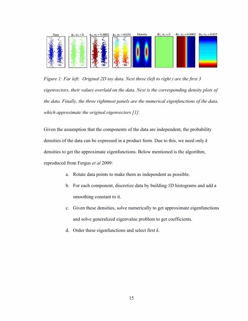
Figure 1: Far left: Original 2D toy data. Next three (left to right ) are the first 3
eigenvectors, their values overlaid on the data. Next is the corresponding density plots of
the data. Finally, the three rightmost panels are the numerical eigenfunctions of the data,
which approximate the original eigenvectors [1].
Given the assumption that the components of the data are independent, the probability
densities of the data can be expressed in a product form. Due to this, we need only k
densities to get the approximate eigenfunctions. Below mentioned is the algorithm,
reproduced from Fergus et al 2009:
a. Rotate data points to make them as independent as possible.
b. For each component, discretize data by building 1D histograms and add a
smoothing constant to it.
c. Given these densities, solve numerically to get approximate eigenfunctions
and solve generalized eigenvalue problem to get coefficients.
d. Order these eigenfunctions and select first k.
16
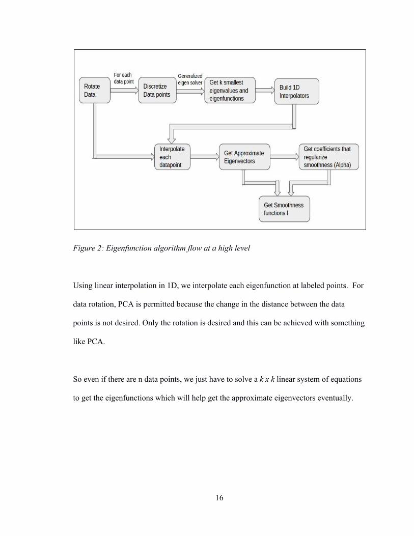
Figure 2: Eigenfunction algorithm flow at a high level
Using linear interpolation in 1D, we interpolate each eigenfunction at labeled points. For
data rotation, PCA is permitted because the change in the distance between the data
points is not desired. Only the rotation is desired and this can be achieved with something
like PCA.
So even if there are n data points, we just have to solve a k x k linear system of equations
to get the eigenfunctions which will help get the approximate eigenvectors eventually.

17
Figure 3: Comparison of Eigenfunction approach and Nystrom Method. Nystrom fails at
low density areas. Eigenfunction approach fails when density is far from product form
(Fergus, 2009, hence the need for an initial rotation step to make the dimensions
independent).
For data above, the eigenfunction approach assumes the input data is linearly separable
over the dimensions. Cases where this assumption fails, the eigenfunction approach does
not work efficiently as shown in the above Fig. 5.
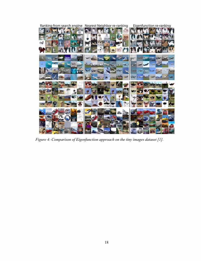
They tested their approach on CIFAR tiny image dataset of 79,302,017 images. They
precomputed k=64 eigenfunctions on the whole dataset and then reduced data dimensions
to 32D. Overall they had 4 classes with 3 pairs of labeled data for each class. In all 12
labeled data.
18
Figure 4: Comparison of Eigenfunction approach on the tiny images dataset [1].
19
CHAPTER 4
SYSTEM ARCHITECTURE AND OVERVIEW
This chapter discusses the architecture for the implemented fit and predict functions. It is
a common practice to implement data science pipelines in this format where model is
trained with a fit function and labels for unseen samples are predicted using a predict
function. The predict function used the trained model parameters from the fit function to
perform prediction. Our implemented pipeline is compatible with the distributed
computing environment Apache Spark. Apache Spark provides a fault-tolerant,
distributed computing environment which can handle huge amount of data because of its
parallelism. It follows a master slave architecture where the execution begins from the
driver machine (Master) and parallel jobs are distributed to worker machines (slaves).
The fit function implements the transductive learning aspect of semi-supervised learning
while the predict function simulates the inductive learning aspect of it. Later we also
discuss the challenges faced during the implementation of the architecture.
20
4.1 Fit Function
The implementation of this approach is programmed with respect to a distributed
paradigm like Apache Spark. The fit function works as per the concept of transductive
learning. It reads in the dataset with labeled as well as unlabeled data points and the
corresponding labels. For unlabeled data points there has to be some dummy label which
will not be counted as a relevant label. The function takes k and number of bins for
discretization as input arguments, where parameter k is the number of dimensions to
work on and number of bins is used to discretize the dimensions of the data points into
histograms.
The function also takes data points and any known labels as input. As per the method, the
data points are rotated doing a full Principal Component Analysis. After performing the
PCA step, we retain all the dimensions, there by fulfilling the assumption that the data
dimensions are independent and orthogonal with respect to each other. At a later point in
the process, we will be required to work on one dimension of the data at a time. Hence
the data which was in the form of a Resilient Distributed Dataset was converted to a more
structured format such as a DataFrame, providing additional tools for inspecting and
analyzing each dimension of the data in parallel. The number of dimensions, d, will
always be far less than the total number of samples. Keeping this assumption in mind, it
is feasible to make use of a structured format like a DataFrame.

21
Figure 5: Flow Process of the fit function

22
Below is the pseudo code:
Figure 6: Pseudo code for the fit function
This structured DataFrame will be primarily used to get the k smallest eigenfunctions and
eigenvalues using the generalized eigensolver. Also, this DataFrame will be later required
to interpolate each data point using the 1D interpolators.
For each dimension of data, we take all data points for that dimension, discretize them by
binning them into a histogram. Here we make use of the number of

23
bins parameter that was given as input to the function. Using the generalized eigensolver
equation in Eigenfunction Approach [1], we obtain the eigenvectors and eigenvalues for
that particular dimension using 𝐷 − 𝑃𝑊𝑃 𝑔 = 𝜎𝑃𝐷𝑔). For each dimension, there will
be a corresponding, most significant, eigenvector and eigenvalue. So for d dimensions,
there will be a (d x bins) vector of eigenvectors and corresponding vector of eigenvalues.
After sorting the d eigenvalues in an ascending order, we select the top k eigenvalues and
their corresponding eigenfunctions.
The next task is to obtain approximate eigenvectors from these k eigenfunctions. Since
we do not build an actual n x n graph Laplacian, we are required to get approximate
eigenvectors. For this purpose, we build 1D straightforward interpolators, one for each
dimension of the data. These interpolators define a density area bounded by the k
eigenfunctions. So once we get these k interpolators, we pass every data point through
these interpolators, interpolate them and get values which are the numerically
approximated eigenvectors. These approximated eigenvectors can be compared to the
actual eigenvectors that we would get using the graph Laplacian. So we are getting the
eigenvectors without having to do a complete n x n computation.
Next in the process we need coefficients that will help regularize the smoothness of the
function such that the data points will fill well into the functions on the manifold. These
coefficients can be obtained by solving the linear equation Σ + 𝑈fΛ𝑈 𝛼 = 𝑈fΛ𝑦 given
in the Fergus et al paper that makes use of these approximated eigenvectors. We denote
these coefficients with α (Alpha).
24
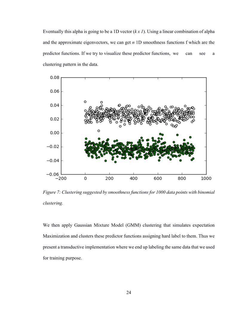
Eventually this alpha is going to be a 1D vector (k x 1). Using a linear combination of alpha
and the approximate eigenvectors, we can get n 1D smoothness functions f which are the
predictor functions. If we try to visualize these predictor functions, we can see a
clustering pattern in the data.
Figure 7: Clustering suggested by smoothness functions for 1000 data points with binomial
clustering.
We then apply Gaussian Mixture Model (GMM) clustering that simulates expectation
Maximization and clusters these predictor functions assigning hard label to them. Thus we
present a transductive implementation where we end up labeling the same data that we used
for training purpose.
25
For the purpose of reuse of parameters and a few variables, Apache Spark provides a
broadcasting facility which enables sharing of variables among the workers. Parameters
like alpha, k, bin edges which could be required on multiple workers are broadcasted for
sharing purpose.
4.2 Predict Function
Predict function implements the inductive learning approach of this algorithm. It takes
new, unobserved data samples as input, uses the trained model parameters, and outputs
labels predicted for the new data. This prediction is performed without using the original
training data, and without rebuilding the model. Data given as input is in the form of
Resilient Distributed Dataset.

26
This data is first rotated using a full PCA (Principal Component Analysis). The rotated
Data is transformed into a structured DataFrame. Then using the interpolators built
during training phase, we interpolate each data point and get the approximate
eigenvectors. It is to be noted here that we eliminate the phase of building interpolators
and getting k
eigenfunctions. Since we reuse these interpolators and k eigenfunctions in the predict
function to predict labels, we call these the learned parameters of the model.
Figure 8: Flow process for predict function
27
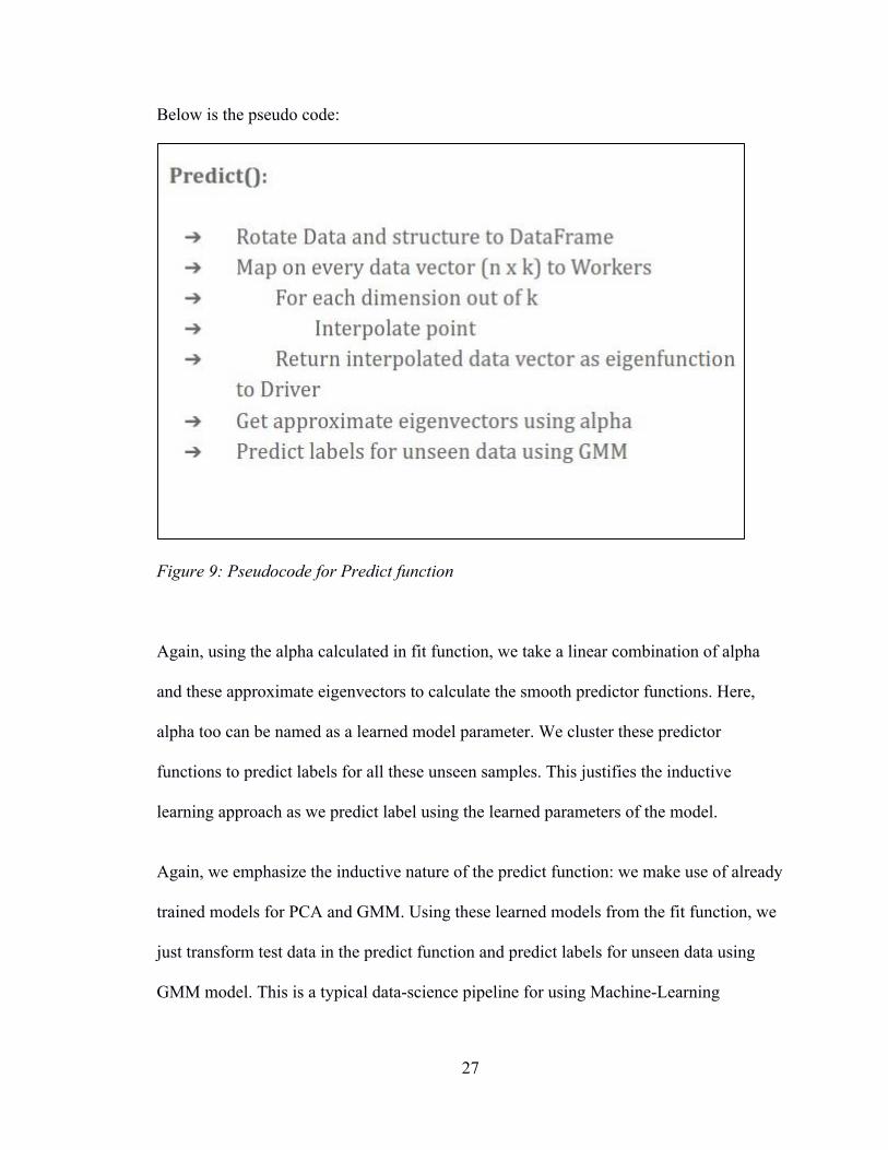
Below is the pseudo code:
Figure 9: Pseudocode for Predict function
Again, using the alpha calculated in fit function, we take a linear combination of alpha
and these approximate eigenvectors to calculate the smooth predictor functions. Here,
alpha too can be named as a learned model parameter. We cluster these predictor
functions to predict labels for all these unseen samples. This justifies the inductive
learning approach as we predict label using the learned parameters of the model.
Again, we emphasize the inductive nature of the predict function: we make use of already
trained models for PCA and GMM. Using these learned models from the fit function, we
just transform test data in the predict function and predict labels for unseen data using
GMM model. This is a typical data-science pipeline for using Machine-Learning

28
Algorithms. Using Python, these functions are made available as a module by the name
“LabelPropagationDistributed”.
4.3 Challenges
This algorithm has been implemented as a combination of functional as well as object
oriented programming paradigms. Apache Spark uses functional programming to
minimize network overhead, whereas well-known machine learning packages such as
Scikit-learn use object-oriented programming to store learned model parameters. But to
provide an implementation in the form of a package, the implementation had to be
modularized. It was challenging to merge both programmatic into a single, standalone
module.
Another challenge was related to the Eigenfunction approach as it was proposed by
Fergus et al 2009. This approach does not discuss the inductive learning aspect of the
algorithm. We were required to interpret and implement the inductive approach. There
were issues for using class functions on the workers. If a function is specific to a class,
sending it to worker sends the class object as well. This is not allowed as Spark cannot
serialize - deserialize it. Solution was to declare them global.
This algorithm requires tweaking of three important parameters namely, k; the
dimensions to work on, bins; the number of bins to build histograms and g; gamma to
calculate affinities using the RBF kernel. We had to experiment to get the right
combination of all three that gave us good results.
29
CHAPTER 5
EIGENFUNCTION APPROACH ANALYSIS
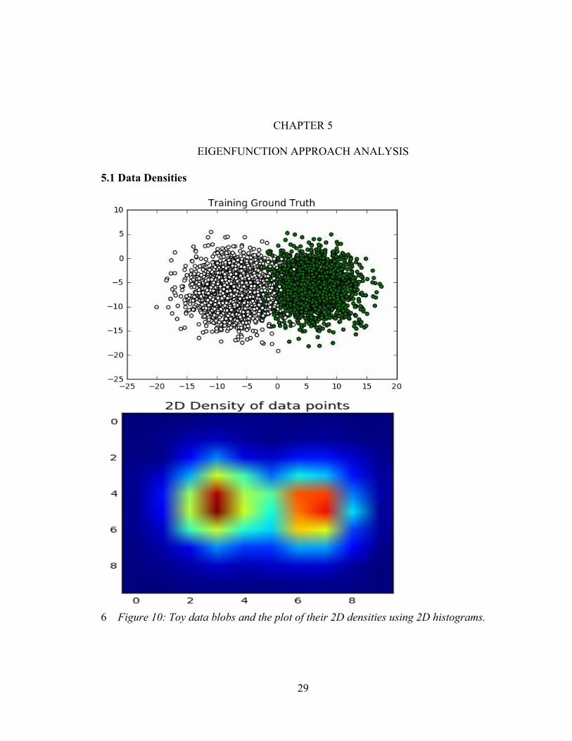
5.1 Data Densities
6 Figure 10: Toy data blobs and the plot of their 2D densities using 2D histograms.

30
Above is the plot of the first two dimensions of a toy dataset and its corresponding data
densities. The dataset consisted of 10000 data points with a suggested 2 class clustering
and 100 dimensions. These densities are the 2D histograms of the data points. This plot is
just to give an idea as to how the interpolators would look like. The interpolators would
be in 1D but this plot is in 2D for visualization purpose. The colors in the density plot
change according to the density of points in that region.
5.2 Data points against Approximate Eigenvectors
Below is the plot of original data points against their approximate eigenvector values.
This eigenvector is the second eigenvector and not the first. Because of minimal
smoothness, the first eigenvector will always be flat.

31
Figure 11: Toy dataset (above) and below is its plot against first Eigenvector for the
data. Zeroth eigenvector will always be flat

32
5.3 Data points against smoothness functions
Below it is the plot of 2D densities of data against the final smoothness operator
functions f. This plot depicts the interpolated area. Any new point can be interpolated into
this density space and its corresponding label can be predicted depending on which
labeled density it is nearer to.
Figure 12: 2D densities of the corresponding toy dataset in the figure above versus its
corresponding smoothness function values
33
CHAPTER 6
RESULTS
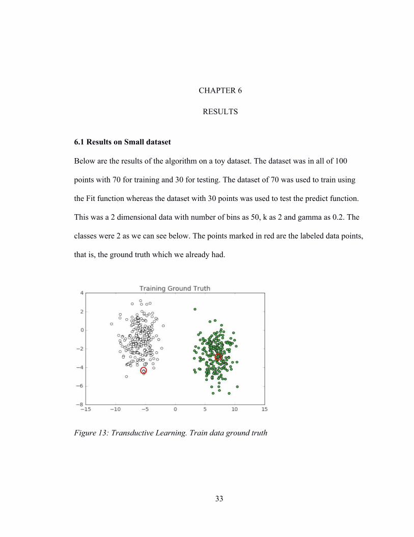
6.1 Results on Small dataset
Below are the results of the algorithm on a toy dataset. The dataset was in all of 100
points with 70 for training and 30 for testing. The dataset of 70 was used to train using
the Fit function whereas the dataset with 30 points was used to test the predict function.
This was a 2 dimensional data with number of bins as 50, k as 2 and gamma as 0.2. The
classes were 2 as we can see below. The points marked in red are the labeled data points,
that is, the ground truth which we already had.
Figure 13: Transductive Learning. Train data ground truth

34
Figure 14: Inductive learning. Test data ground truth
Figure 15: Transductive learning. Train data predicted labels

35
Figure 16: Inductive learning. Test data predicted labels.
Given the 2 labeled data points out of 70, it can be seen that the algorithm could label all
70 points correctly and the predict function could also label all the unseen 30 points with
the same accuracy.
6.2 Results on Bigger Dataset
We then tried to use a dataset closer to a real-world scenario. The dataset size was 60000
with 10 classes and 100 dimensions. This dataset was a potential simulation to the olfactory
dataset with 10 classes and 100 dimensions. (Though we will be dealing with 146
dimensions). Looking at the data distribution we decided to use a k of 20, number of bins
as 2000 and a gamma for RBF kernel as 0.01. This algorithm is very sensitive to gamma,
then bins and then k. Gamma decides the extent to which the label should be propagated.
Out of the 60000 data, 54000 was training data and 6000 was for testing.
36
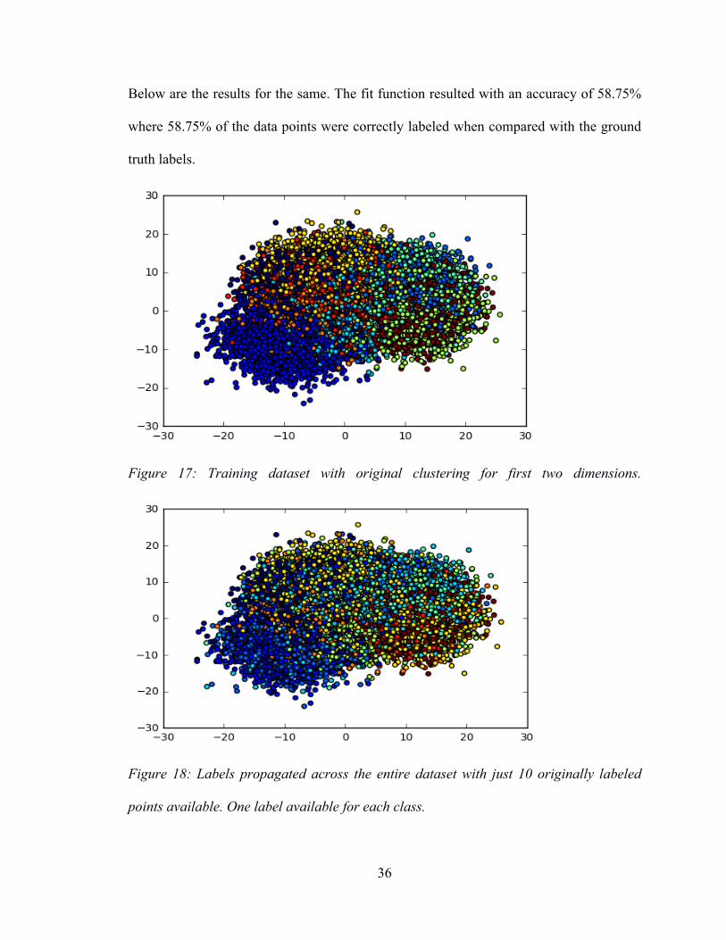
Below are the results for the same. The fit function resulted with an accuracy of 58.75%
where 58.75% of the data points were correctly labeled when compared with the ground
truth labels.
Figure 17: Training dataset with original clustering for first two dimensions.
Figure 18: Labels propagated across the entire dataset with just 10 originally labeled
points available. One label available for each class.

37
Figure 19: Test data set original clustering for first two dimensions.
Figure 20: Label propagation after 1D interpolation of data using the learned model
parameters during the training phase. This depicts the Inductive Learning.
38
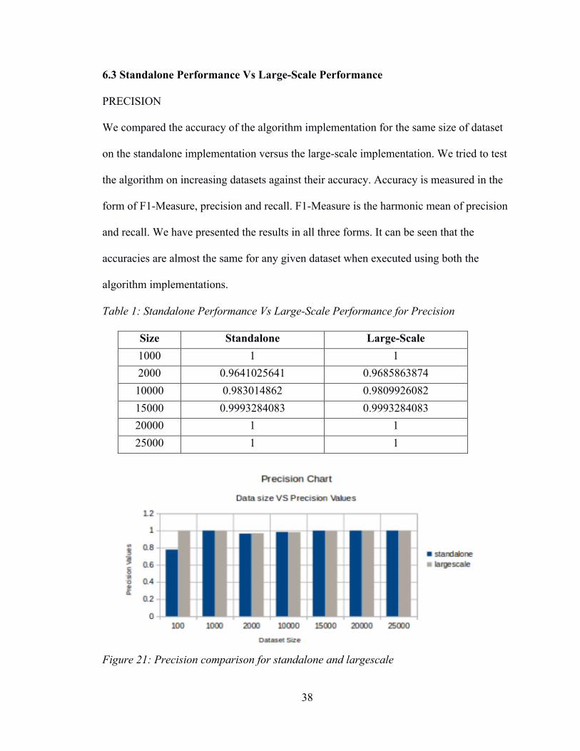
6.3 Standalone Performance Vs Large-Scale Performance PRECISION We compared the accuracy of the algorithm implementation for the same size of dataset
on the standalone implementation versus the large-scale implementation. We tried to test
the algorithm on increasing datasets against their accuracy. Accuracy is measured in the
form of F1-Measure, precision and recall. F1-Measure is the harmonic mean of precision
and recall. We have presented the results in all three forms. It can be seen that the
accuracies are almost the same for any given dataset when executed using both the
algorithm implementations.
Table 1: Standalone Performance Vs Large-Scale Performance for Precision
Size Standalone Large-Scale 1000 1 1 2000 0.9641025641 0.9685863874 10000 0.983014862 0.9809926082 15000 0.9993284083 0.9993284083 20000 1 1 25000 1 1
Figure 21: Precision comparison for standalone and largescale
39
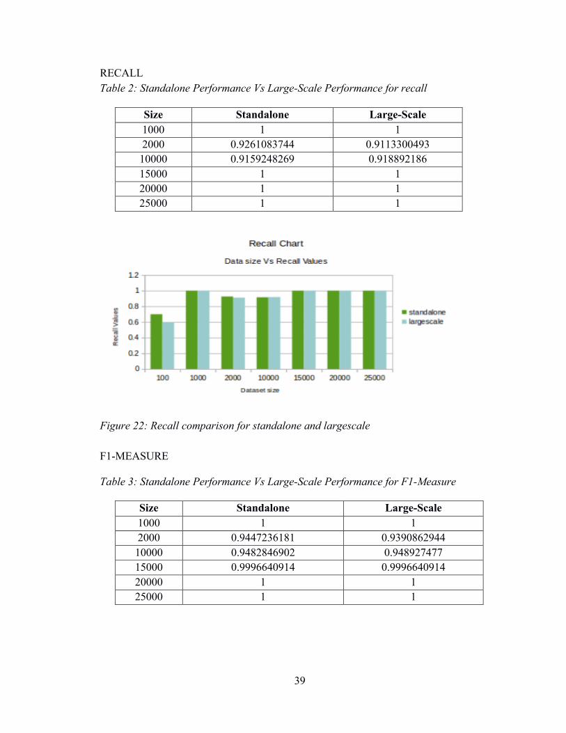
RECALL Table 2: Standalone Performance Vs Large-Scale Performance for recall
Size Standalone Large-Scale 1000 1 1 2000 0.9261083744 0.9113300493 10000 0.9159248269 0.918892186 15000 1 1 20000 1 1 25000 1 1
Figure 22: Recall comparison for standalone and largescale
F1-MEASURE
Table 3: Standalone Performance Vs Large-Scale Performance for F1-Measure
Size Standalone Large-Scale 1000 1 1 2000 0.9447236181 0.9390862944 10000 0.9482846902 0.948927477 15000 0.9996640914 0.9996640914 20000 1 1 25000 1 1

40
Figure 23: F1-Measure comparison for standalone and largescale
6.4 Parameters vs. Accuracy
Here we try to tweak parameters like gamma, k and number of bins and compare the
results with the accuracy. These parameters are very sensitive to the accuracy that we
get. Starting with gamma, gamma is the RBF kernel affinity coefficient. The gamma
decides the extent of label propagation towards its neighbors. The more scattered the
intra-cluster points, the smaller gamma should be. Gamma corresponds to negative
inverse of sigma in the RBF kernel. Parameter k decides how many dimensions to
actually work on. The k dimensions are selected looking at the ordered eigenvalues. If the
selected k is very large then a lot of noise gets introduced. If the k is very small the
meaningful dimensions are not selected giving a bad clustering. Number of Bins depends
on the data size to be dealt with. For each dimension we build histograms. So depending
on the total data points, we can select number of bins for discretization. Few bins may not
give a detailing of the densities. A larger number for bins may cause some bins to be
empty thus again, not having a fair distribution. This algorithm needs a lot of tweaking
41
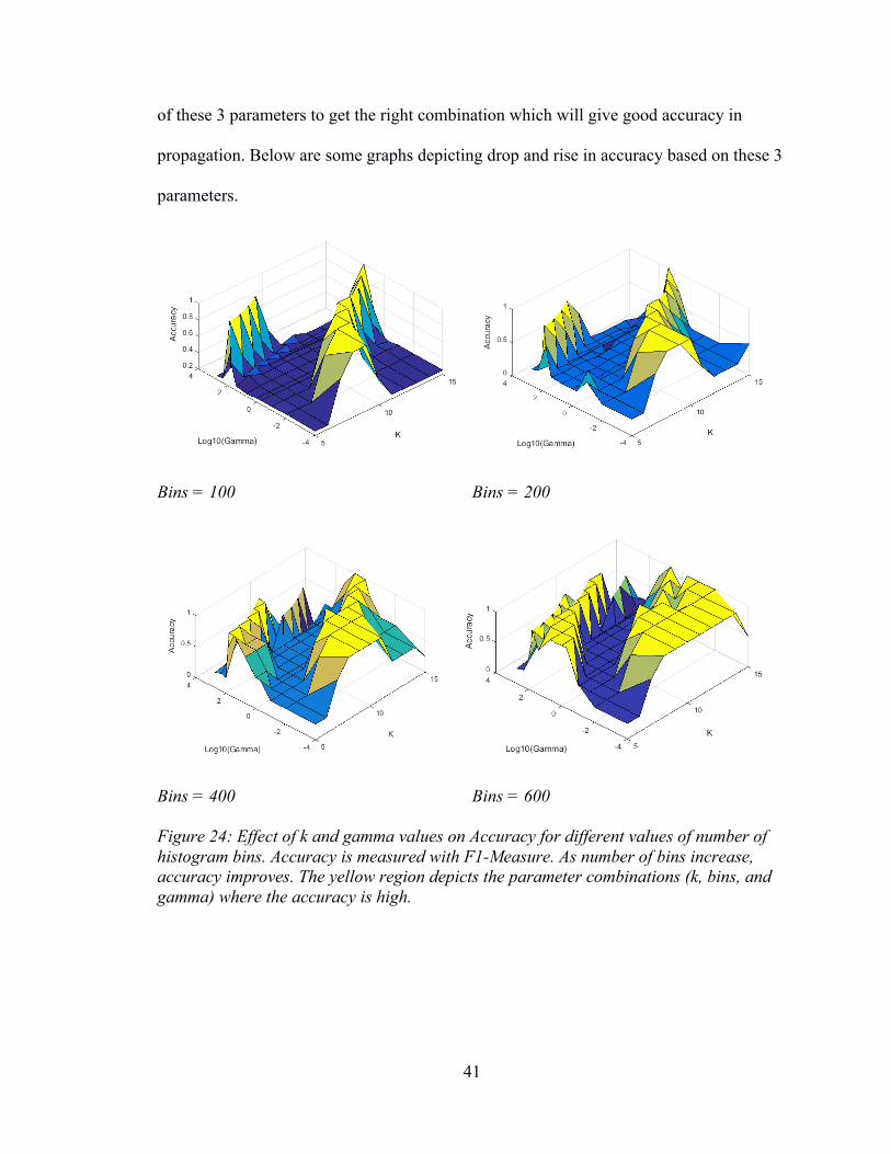
of these 3 parameters to get the right combination which will give good accuracy in
propagation. Below are some graphs depicting drop and rise in accuracy based on these 3
parameters.
Bins = 100 Bins = 200
Bins = 400 Bins = 600
Figure 24: Effect of k and gamma values on Accuracy for different values of number of histogram bins. Accuracy is measured with F1-Measure. As number of bins increase, accuracy improves. The yellow region depicts the parameter combinations (k, bins, and gamma) where the accuracy is high.
42
It can be observed that as the number of bins increases, there seems to be more surface
area (combination of gamma and k) that gives perfect accuracy. There is likely some
threshold to this. But if the number of bins is increased beyond the threshold, the
performance degrades.
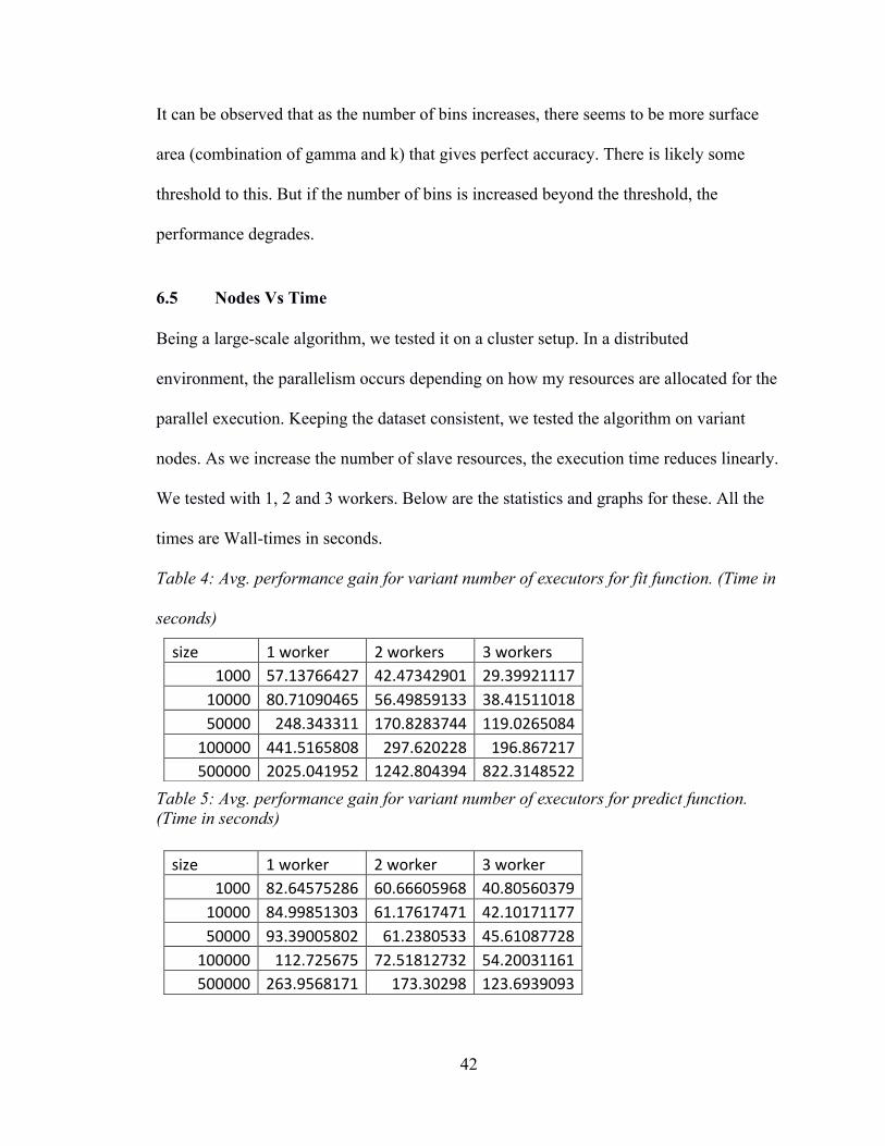
6.5 Nodes Vs Time
Being a large-scale algorithm, we tested it on a cluster setup. In a distributed
environment, the parallelism occurs depending on how my resources are allocated for the
parallel execution. Keeping the dataset consistent, we tested the algorithm on variant
nodes. As we increase the number of slave resources, the execution time reduces linearly.
We tested with 1, 2 and 3 workers. Below are the statistics and graphs for these. All the
times are Wall-times in seconds.
Table 4: Avg. performance gain for variant number of executors for fit function. (Time in
seconds)
Table 5: Avg. performance gain for variant number of executors for predict function. (Time in seconds)
size 1worker 2worker 3worker1000 82.64575286 60.66605968 40.8056037910000 84.99851303 61.17617471 42.1017117750000 93.39005802 61.2380533 45.61087728
100000 112.725675 72.51812732 54.20031161500000 263.9568171 173.30298 123.6939093
size 1worker 2workers 3workers1000 57.13766427 42.47342901 29.3992111710000 80.71090465 56.49859133 38.4151101850000 248.343311 170.8283744 119.0265084100000 441.5165808 297.620228 196.867217500000 2025.041952 1242.804394 822.3148522
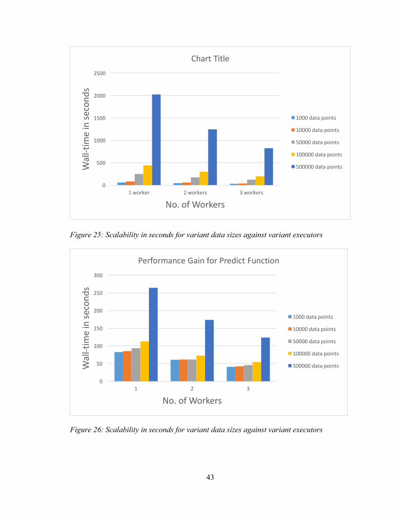
43
Figure 25: Scalability in seconds for variant data sizes against variant executors
Figure 26: Scalability in seconds for variant data sizes against variant executors
0
500
1000
1500
2000
2500
1worker 2workers 3workers
Wall-tim
einse
cond
s
No.ofWorkers
ChartTitle
1000datapoints
10000datapoints
50000datapoints
100000datapoints
500000datapoints
0
50
100
150
200
250
300
1 2 3
Wall-tim
einse
cond
s
No.ofWorkers
PerformanceGainforPredictFunction
1000datapoints
10000datapoints
50000datapoints
100000datapoints
500000datapoints
44
CHAPTER 7
POTENTIAL USE CASE: COMPUTATIONAL OLFACTION
This chapter talks about the work done in olfaction so far. It talks about 3 different
research work that will establish a ground truth for our work.
7.1 Introduction
The common dictionary definition of Olfaction is “sense of smell”. There can be
disagreements in the descriptions of smells given by people. The perception of an odor
for every person could be different as odors highly rely on hundreds of receptors in the
brain. This concept is defined by the term Structure-Odor Relationship. It is difficult to
map the physicochemical properties of Odors to perceptual representations[16]. The
physicochemical properties are quantifiable, objective chemical properties of the
molecule in question; e.g., color, texture, odor, number of atoms, melting point, boiling
point and so on. Deriving a quantifiable mapping between these physicochemical
properties and their resulting odor percepts is the driving question behind computational
olfaction, and an ideal candidate for machine learning.
To achieve this, we choose the approach of applying Machine Learning techniques to
map the physicochemical properties of chemical substances to the odor perceptual space.
Machine Learning provides a statistically sound predictive analysis for the data which
45
can be fairly trusted. Machine Learning has even proved its significance in numerous
Healthcare prediction problems.
Our approach follows the semi-supervised learning pattern to do the desired mapping: it
is expensive to acquire ground-truth perceptual odor descriptors for molecules, and
impossible to do on a large scale. On the other hand, it is comparatively easy to derive
physicochemical properties of small molecules. Thus, we are left in a situation with a
large amount of unlabeled data and a small amount of labeled data, and need to learn a
model: an ideal situation for semi-supervised learning.
There are data patterns that indicate the type of machine learning approach that can be
undertaken to solve the issue at hand. In regards to that, looking at the data pattern that
we are dealing with, semi-supervised learning approach may seem to work a lot better
than either supervised or unsupervised learning approach alone. Another good reason to
use ML approach is the availability of data characteristics. Data characteristics can be
named as “features” in terms of Machine Learning language. The physicochemical
properties are the features for our olfaction data.
The focus of this topic is on scaling the approach for huge amount of data. Given a set of
Billions of chemical substances each with hundreds of physicochemical properties our
large scale semi supervised approach can handle such huge amount of dataset. Being a
generic algorithm, it is compatible with any real time dataset.

46
7.2 Computational Olfaction – Background
7.2.1 “Odor quality: semantically generated multidimensional profiles are stable”
[5]
This paper talks about characterization of odors of 10 known compounds by 150 subjects
using a list of 146 descriptors. There are two methods for identification of odor, reference
odorant method and semantic method. As the name suggests, reference odorant method
finds a reference to a similar odor whereas semantic method is to define or describe odor
in terms of words. Around 150 subjects were asked to provide with a combination of
descriptors for the 10 odorants. This combination was chosen out of the 146 descriptors
given to them. A few of these 146 descriptors are Fruity, citrus, Lemon, Grapefruit,
Orange, Fruity, non-citrus, Pineapple, Grape juice. The subjects were asked to provide
scores for descriptors which they felt would be an appropriate combination for each of
the 10 odorants. The score of every descriptor and the frequency of every descriptor were
the deciding factors for the characterization of the odorants. The list of the 10 odorants is
as follows: Acetophenone, Anethole, I-Butanol, I-Carvone, p-Cresylmethylether,
Cyclohexanol, I-Heptanol, I-Hexanol, Phenylethanol, Pyridine.
7.2.2 “In search of the structure of human olfactory space” [6]
This paper investigates the structure of olfactory space defined by the responses of 150
human observers. They make use of responses for 144 odorants and represent it in a set
of 146D vectors. These 146 dimensions are the descriptors that were established in the
paper by Dravnieks(AOCP, 1985). Here they apply a PCA (Principal Component
Analysis) on these odorants thereby reducing the dimensionality to a 2D curved surface

47
which accommodates the 144 odorants. For 2D approximation, they relate the 2
parameters to the physicochemical parameters of odorant molecules. They also show that
one of these parameters is related to the eigenvalues of molecules connectivity matrix,
while the other is correlated with measures of molecules polarity[6]. The paper also
established a mapping for the odour perceptual space and the physicochemical properties.
They compared the resulting two co-ordinates to various physicochemical properties of
odorants. They eventually worked with 126 physicochemical properties and established
the correlation of these properties with the 2 perceptual dimensions.
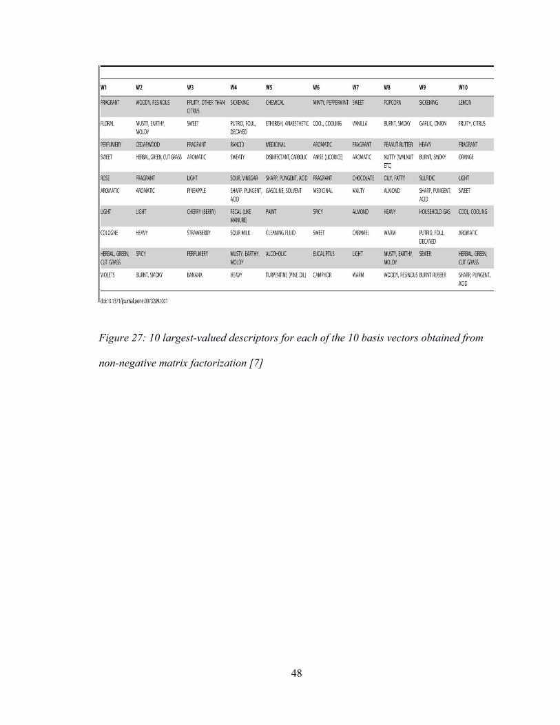
7.2.3 “Categorical Dimensions of Human Odor Descriptor Space Revealed by
Non- Negative Matrix Factorization” [7]
This paper talks about reducing the dimensions of odorants using a Non-Negative Matrix
factorization to uncover the structure in a panel of odor profiles. Each odor is defined as a
combination of these 146 descriptors. The paper also corroborates the theory that odor
dimensions apply categorically; that the odor space is defined in a discrete and
intrinsically clustered manner. They choose the NMF approach for dimensionality
reduction based on the observation that all the descriptor values are non-negative. They
reduce the 146 dimensional space to a 10 dimensional perceptual space. They worked on
144 monomolecular odors each represented as a 146 dimensional (descriptor) vector.
48
Figure 27: 10 largest-valued descriptors for each of the 10 basis vectors obtained from
non-negative matrix factorization [7]
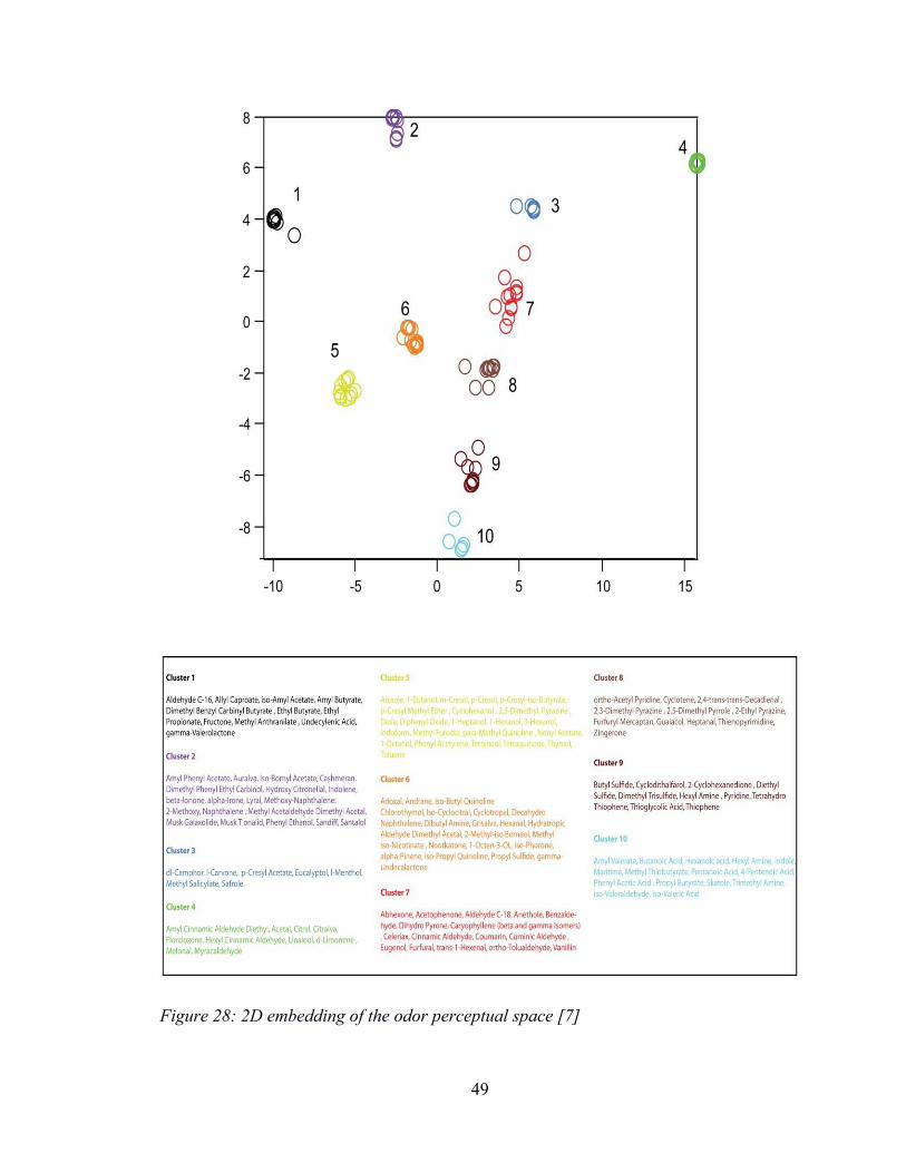
49
Figure 28: 2D embedding of the odor perceptual space [7]

50
7.3 Challenges
1. Due to difficulty in interpretation of odors for chemical components, the known
mappings for physicochemical features to components are very few. There is not enough
established data available.
2. Moreover, it is impractical to manually identify odors of compounds for several
reasons one of which being that it may be hazardous to do so. This strongly explains need
for computational olfaction identification.
3. The semi-supervised approach given by Fergus et al makes a strong assumption that
the data dimensions are as independent as possible. This won’t be the case when dealing
with olfaction dataset. The olfaction data is supposed to be a very high dimensional data.
It is unlikely that the dimensions will be independent.
If we are able to find a numerical workaround to achieve independent dimensionality, we
can apply eigenfunction approach to olfaction data.
51
CHAPTER 8
CONCLUSION
We have provided a large scale implementation of the eigenfunction approach using
semi-supervised learning on a distributed framework like Apache Spark. We have
discussed the transductive and inductive learning approaches provided by this approach.
The approach implementation that we provide simulates the transductive as well as
inductive parts of it. We have analyzed the eigenfunction approach and presented this
analysis with the help of density plots. We have also discussed the background of
computational olfaction and how this approach would be compatible with the olfaction
data. We have presented this algorithm results on toy datasets and also analyzed the
process. The main idea is to be able to apply this algorithm on large datasets. The
motivation for this work was computational olfaction. The next step would be applying
this algorithm on the olfaction data. The olfaction data is a data with 10 odor classes and
is high-dimensional. If the dataset is dimensionally independent and proportionally
labeled, an algorithm like eigenfunction can be aptly applied to such high dimensional
data. Moreover, since this algorithm is linear with respect to the number of data points,
the time required will be definitely lesser than that required by methods that construct a
full n x n graph Laplacian. Given any such high-dimensional, dimensionally independent
dataset with an appropriate proportion of labeled and unlabeled data, this algorithm can
52
be used to predict labels for the unlabeled points by its transductive method and can also
label any new unseen point by its inductive method.
The Eigenfunction approach is efficient in terms of computation time required but it lacks
robustness since it is very sensitive to the three parameters k, bins, and gamma. A lot of
tweaking is required if the data distribution and data pattern is unknown. But if we can
study the data distribution, the clustering depicted by the ground truth, then it will be
easier tweaking the parameters.
53
REFERENCES
1. R. Fergus, A. Torralba, and Y. Weiss. Semi-supervised learning in gigantic image
collections. In NIPS, 2009.
2. Zhu, Xiaojin. Semi-Supervised Learning, University of Wisconsin-Madison, 2006
3. A. Subramanya and P. P. Talukdar, “Graph-based semi-supervised learning
algorithms for NLP”, Tutorial Abstracts of ACL 2012, Association for Computational
Linguistics, pp. 6-6, 2012.
4. Chapelle, Olivier; Schölkopf, Bernhard; Zien, Alexander (2006). Semi-supervised
learning. Cambridge, Mass.: MIT Press. ISBN 978-0-262-03358-9.
5. Dravnieks A (1982) Odor quality: semantically generated multi-dimensional
profiles are stable. Science 218:799-801.
6. Koulakov, A. A., Kolterman, B. E., Enikolopov, A. G., & Rinberg, D. (2011). In
search of the structure of human olfactory space. Frontiers in Integrative Neuroscience, 5,
65.
7. Castro, J.B., Ramanathan, A., Chennubhotla, C.S., 2013. Categorical dimensions
of human odor descriptor space revealed by non-negative matrix factorization. PLoS One
8, e73289.
8. Zhu, Xiaojin. Semi-Supervised Learning, Springer, 2010.
9. Zhu, X., Ghahramani, Z., & Lafferty, J. (2003a). Semi-supervised learning using
Gaussian fields and harmonic functions. The 20th International Conference on Machine
Learning (ICML).

54
10. X. Zhu. Semi-supervised learning literature survey. Computer Sciences Technical
Report 1530, University of Wisconsin–Madison, 2005b.
11. X. Zhu and A. B. Goldberg, Introduction to semi-supervised learning. Morgan &
Claypool Publishers, 2009.
12. Zhu, Xiaojin and Zoubin Ghahramani. Learning from labeled and unlabeled data
with label propagation. School Comput. Sci., Carnegie Mellon Univ., Pittsburgh, PA,
Tech. Rep. CMU-CALD-02-107, 2002.
13. Christiane Linster, Computational Olfaction, Springer, 2014
14. Zhang, K., Kwok, J. T., and Parvin, B. Prototype vector machine for large scale
semi- supervised learning. In Proc. ICML, 2009
15. Liu, W., He, J., and Chang, S.-F. Large graph construction for scalable semi-
supervised learning. In Proc. ICML, 2010.
16. R.Kumar ,R. Kaur ,B. Auffarth ,A. Bhondekar, Understanding the Odour Spaces:
A Step towards Solving Olfactory Stimulus-Percept Problem, 2015.
17. U. Raghavan, R. Albert, S. Kumara, Near linear time algorithm to detect
community structures in large-scale networks,2007.
18. A. P. Dempster; N. M. Laird; D. B. Rubin, Maximum Likelihood from
Incomplete Data via the EM Algorithm, 1977.