Large Scale Kernel Regression via Linear Programming

Machine Learning, 46, 255–269, 2002c© 2002 Kluwer Academic Publishers. Manufactured in The Netherlands.

Large Scale Kernel Regressionvia Linear Programming

O.L. MANGASARIAN [email protected] Sciences Department, University of Wisconsin, 1210 West Dayton Street, Madison, WI 53706, USA

DAVID R. MUSICANT [email protected] of Mathematics and Computer Science, Carleton College, One North College Street, Northfield,MN 55057, USA

Editor: Nello Cristianini

Abstract. The problem of tolerant data fitting by a nonlinear surface, induced by a kernel-based support vectormachine is formulated as a linear program with fewer number of variables than that of other linear programmingformulations. A generalization of the linear programming chunking algorithm for arbitrary kernels is implementedfor solving problems with very large datasets wherein chunking is performed on both data points and problem vari-ables. The proposed approach tolerates a small error, which is adjusted parametrically, while fitting the given data.This leads to improved fitting of noisy data (over ordinary least error solutions) as demonstrated computationally.Comparative numerical results indicate an average time reduction as high as 26.0% over other formulations, witha maximal time reduction of 79.7%. Additionally, linear programs with as many as 16,000 data points and morethan a billion nonzero matrix elements are solved.

Keywords: kernel regression, support vector machines, linear programming

1. Introduction

Tolerating a small error in fitting a given set of data, i.e. disregarding errors that fall withinsome positive ε, can improve testing set correctness over a standard zero tolerance errorfit (Street & Mangasarian, 1998). Vapnik (1995, Section 5.9) makes use of Huber’s robustregression ideas (Huber, 1964) by utilizing a robust loss function (Vapnik, 1995, p. 152)with an ε-insensitive zone (figure 1 below) and setting up linear and quadratic programsfor solving the problem. Scholkopf et al. (1998, 1999) use quadratic-programming-basedsupport vector machines to automatically generate an ε-insensitive “tube” around the datawithin which errors are discarded. In Smola, Scholkopf, and Ratsch (1999), they use alinear programming (LP) based support vector machine approach for ε-insensitive approx-imation. An LP formulation has a number of advantages over the quadratic programming(QP) based approach given by Vapnik (1995), most notably sparsity of support vectors(Bennett, 1999; Weston et al., 1999; Smola, 1998) and the ability to use more generalkernel functions (Mangasarian, 2000). In this work we simplify the linear programmingformulation of Smola, Scholkopf, and Ratsch (1999) by using a fewer number of vari-ables. This simplification leads to considerably shorter computing times as well as a more

256 O.L. MANGASARIAN AND D.R. MUSICANT

Figure 1. One dimensional loss function minimized.

efficient implementation of a generalization of the linear programming chunking algorithmof Bradley and Mangasarian (2000) for very large datasets. This generalization consists ofchunking both data points and problem variables (row and column chunking) which allowsus to solve linear programs with more than a billion nonzero matrix elements.

We briefly outline the contents of the paper. In Section 2 we derive and give the theoreticaljustification of our linear programming formulation (7) based on the loss function of figure 1and show (Lemma 2.1) that it is equivalent to the linear program (9) of Smola, Scholkopf, andRatsch (1999) but with roughly 75% of the number of variables. Proposition 2.2 shows thatthe tolerated error interval length 2ε varies directly with the size of the parameter µ ∈ [0, 1]of our linear program (7), where µ = 0 corresponds to a least 1-norm fit of the data (8)while the value µ = 1 disregards the data and is therefore meaningless. It turns out, thatdepending on the amount of noise in the data, some positive value of µ < 1 gives a best fitas indicated by the computational results summarized in Table 1. Section 3 implements andtests our linear programming formulation (7) and compares it with the linear programmingformulation (9) of Smola, Scholkopf, and Ratsch (1999). Our formulation yielded an averagecomputational time reduction as high as 26.0% on average, with a maximal time reduction of79.7%. Our chunking implementation solved problems with as many as 16,000 observations.By contrast the largest dataset attempted in Smola, Scholkopf, & Ratsch (1999) contained506 points.

To summarize, there are three main results in this paper. We present a kernel regressiontechnique as a linear program which runs faster than previous techniques available. We intro-duce a simultaneous row-column chunking algorithm to solve this linear program. Finally,we demonstrate that this row-column chunking algorithm can be used to significantly scaleup the size of problem that a given machine can handle.

A word about our notation. All vectors will be column vectors unless transposed to a rowvector by a prime superscript ′. For a vector x in the d-dimensional real space Rd , the plusfunction x+ is defined as (x+)i = max {0, xi }, i = 1, . . . , d. The scalar (inner) product oftwo vectors x and y in the d-dimensional real space Rd will be denoted by x ′y. For an ×dmatrix A, Ai will denote the i th row of A. The identity matrix in a real space of arbitrarydimension will be denoted by I , while a column vector of ones of arbitrary dimension willbe denoted by e. For A ∈ R×d and B ∈ Rd×, the kernel K (A, B) maps R×d × Rd× into

LARGE SCALE KERNEL REGRESSION 257

R×. In particular if x and y are column vectors in Rd then, K (x ′, A′) is a row vector inR, K (x ′, y) is a real number and K (A, A′) is an × matrix. Note that K (A, A′) will beassumed to be symmetric, that is K (A, A′) = K (A, A′)′. The 1- 2- and ∞-norms will bedenoted by ‖·‖1, ‖·‖2 and ‖·‖∞, respectively.

2. The support vector regression problem

We consider a given dataset of points in d dimensional real space Rd represented by thematrix A ∈ R×d . Associated with each point Ai is a given observation, a real number yi ,i = 1, . . . , . We wish to approximate y ∈ R by some linear or nonlinear function of thematrix A with linear parameters, such as the simple linear approximation:

Aw + be ≈ y, (1)

where w ∈ Rd and b ∈ R1 are parameters to be determined by minimizing some error crite-rion. If we consider w to be a linear combination of the rows of A, i.e. let w = A′α, α ∈ R,then we have:

AA′α + be ≈ y. (2)

This immediately suggests the much more general idea of replacing the linear kernel AA′ bysome arbitrary nonlinear kernel K (A, A′) : R×d × Rd× → R× that leads to the followingapproximation, which may be nonlinear in A but linear in α:

K (A, A′)α + be ≈ y. (3)

We will measure the error in (3) by a vector s ∈ R defined by:

−s ≤ K (A, A′)α + be − y ≤ s, (4)

which we modify by tolerating a small fixed positive error ε, possibly to overlook errors inthe observations y, as follows:

−s ≤ K (A, A′)α + be − y ≤ s

eε ≤ s(5)

We now drive the error s no lower than the fixed (for now) tolerance ε by minimizing the1-norm of the error s together with the 1-norm of α for complexity reduction or stabilization.This leads to the following constrained optimization problem with positive parameter C :

min(α,b,s)

1‖α‖1 + C

‖s‖1

s.t. −s ≤ K (A, A′)α + be − y ≤ s

eε ≤ s,

(6)

which can be represented as a linear program. For a linear kernel and a fixed tolerance ε, thisis essentially the model proposed in Street and Mangasarian (1998), which utilizes a 2-norminstead of a 1-norm. We now allow ε to be a a nonnegative variable in the optimizationproblem above that will be driven to some positive tolerance error determined by the size of


the parameter µ. By making use of linear programming perturbation theory (Mangasarian& Meyer, 1979) we parametrically maximize ε in the objective function with a positiveparameter µ to obtain our basic linear programming formulation of the nonlinear supportvector regression (SVR) problem:

min(α,b,s,ε,a)

1

e′a + C

e′s − Cµε

s.t. −s ≤ K (A, A′)α + be − y ≤ s

0 ≤ eε ≤ s,

−a ≤ α ≤ a.

(7)

For µ = 0 this problem is equivalent to the classical stabilized least 1-norm error mini-mization of:

min(α,b)

‖α‖1 + C‖K (A, A′)α + be − y‖1. (8)

For positive values of µ, the zero-tolerance ε of the stabilized least 1-norm problem isincreased monotonically to ε = ‖y‖∞ when µ = 1. (See Proposition 2.2 below.) Compo-nents of the error vector s are not driven below this increasing value of the tolerated error ε.Thus, as µ increases from 0 to 1, ε increases correspondingly over the interval [0, ‖y‖∞].Correspondingly, an increasing number of error components (K (A, A′)α + be − y)i , i =1, . . . , , fall within the interval [−ε, ε] until all of them do so when µ = 1 and ε = ‖y‖∞.(See Proposition 2.2 below.)

One might criticize this approach by pointing out that we have merely substituted oneexperimental parameter (ε in (6)) for another parameter (µ in (7)). This substitution, how-ever, has been shown both theoretically and experimentally to provide tighter control ontraining errors (Scholkopf et al., 1999; Vapnik, 1995). It has also been suggested that inmany applications, formulation (7) may be more robust (Scholkopf et al., 1999).

It turns out that our linear program (7) is equivalent to the one proposed by Smola,Scholkopf, and Ratsch (1999):

min(α1,α2,b,ξ 1,ξ 2,ε)

1

e′(α1 + α2) + C

e′(ξ 1 + ξ 2) + C(1 − µ)ε

s.t. −ξ 2 − eε ≤ K (A, A′)(α1 − α2) + be − y ≤ ξ 1 + eε

α1, α2, ξ 1, ξ 2, ε ≥ 0,

(9)

with 4 + 2 variables compared to our 3 + 2 variables. We now show that the two problemsare equivalent. Note first that at optimality of (9) we have that α1′

α2 = 0. To see this, letα = α1 − α2. Consider a particular component αi at optimality. If αi > 0, then α1

i = αi

and α2i = 0 since we minimize the sum of α1 and α2 in the objective function. By a similar

argument, if αi < 0, then α2i = −αi and α1

i = 0. Hence for α = α1 − α2 it follows that|α| = α1 + α2. We thus have the following result.

Lemma 2.1 (LP Equivalence). The linear programming formulations (7) and (9) areequivalent.


Proof: Define the deviation error:

d = K (A, A′)α + be − y. (10)

By noting that at an optimal solution of (9), ξ 1 = max{d − eε, 0} = (d − eε)+ and ξ 2 =max{−d − eε, 0} = (−d − eε)+, the linear program (9) can be written as:

min(α,b,ε,d)

1

‖α‖1 + C

(e′(d − eε)+ + e′(−d − eε)+) + C(1 − µ)ε, (11)

or equivalently

min(α,b,ε,d)

1

‖α‖1 + C

e′(|d| − eε)+ + C(1 − µ)ε. (12)

On the other hand, note that at optimality the variable s of the linear program (7) is givenby:

s = max{|d|, eε} = eε + max{|d| − eε, 0} = eε + (|d| − eε)+. (13)

Thus the linear program (7) becomes, upon noting that e′e

= 1:

min(α,b,ε,d)

1

‖α‖1 + C

e′(|d| − eε)+ + C(1 − µ)ε, (14)

which is identical to (12). ✷

Note that (14) is equivalent to:

min(α,b,ε,d)

1

‖α‖1 + C

(‖(|d| − eε)+‖1 + (1 − µ)ε), (15)

and figure 1 depicts the loss function (‖(|d|−eε)+‖1 +(1−µ)ε) of (15) as a function of aone dimensional error d with = 1. The loss function is being minimized by the equivalentlinear programs (7) and (9). The linear program (7) generates a tolerance ε ∈ [0, ‖y‖∞]corresponding to the parameter µ ∈ [0, 1]. Within the increasing-size interval [−ε, ε],depicted in figure 1, an increasing number of errors corresponding to the constraints of (7)fall, i.e.:

−ε ≤ (K (A, A′)α + be − y)i ≤ ε, i ∈ I ⊂ {1, . . . , }.

By using linear programming perturbation theory we can give a useful interpretation ofthe role of the parameter (1 −µ) appearing in the formulations above. We note first that theparameter µ lies in the interval [0, 1]. This is so because for µ > 1 the objective functionof the linear program (9) is unbounded below (let ε go to ∞), while for negative µ it is


Figure 2. Visual representation of Proposition 2.2. The interval [0, 1] is shown, with µ and µ indicated as well.The roman numerals indicate which part of Proposition 2.2 is relevant.

evident from the linear program (7) that ε = 0 and we revert to the stabilized least one normformulation (8).

Proposition 2.2 (Perturbation parameter interpretation).

(i) For µ = 0 the linear program (7) is equivalent to the classical stabilized least 1-normapproximation problem (8).

(ii) For all µ ∈ [0, µ] for some fixed µ ∈ (0, 1], we obtain a fixed solution of the stabilizedleast 1-norm approximation (8) as in (i) with the ADDITIONAL property of maximizingε, the least error component. Hence ε is fixed over the interval µ ∈ [0, µ].

(iii) For all µ ∈ [µ, 1] for some fixed µ in [0, 1), we obtain a fixed solution of

min(α,b,ε,d)

1

‖α‖1 + C

e′(|d| − eε)+ (16)

with the ADDITIONAL property of minimizing ε, the least error component. Hence ε isfixed over the interval µ ∈ [µ, 1].

(iv) For µ ∈ [0, 1] we get a monotonically nondecreasing least error component ε de-pendent on µ until the value µ = 1 is reached whereat all error components havebeen trapped within the interval [−ε, ε] with the trivial solution: α = 0, b = 0, ε =‖y‖∞, s = eε.

Proof:

(i) Because a ≥ 0, s ≥ 0 and ε is absent from the objective function of (7), ε can be setto zero and the resulting problem is that of minimizing the stabilized classical least1-norm approximation (8).

(ii) We first note that the linear program (7) is solvable for all µ ∈ [0, 1] because itsobjective function is bounded below by zero on its nonempty feasible region asfollows:

1

e′a + C

e′s − Cµε = 1

e′a + C

e′(s − µeε)

≥ 1

e′a + C

e′(s − eε) ≥ 0. (17)

The desired result is then a direct consequence of Mangasarian and Meyer (1979,Theorem 1), Theorem 1 which states that for all sufficiently small perturbations of


a linear programming objective function by another possibly nonlinear function, asolution of the linear program is obtained that in addition optimizes the perturbationfunction as well. This translates here to obtaining a solution of the stabilized least1-norm approximation problem (8) that also maximizes ε.

(iii) We observe that the linear program (7) is equivalent to the linear program (12), asshown in Lemma 2.1. We therefore obtain result (iii) by a similar application of linearprogramming perturbation theory as in (ii). Thus for µ = 1 the linear program (12)is equivalent to (16) and for µ sufficiently close to 1, that is µ ∈ [µ, 1] for someµ ∈ [0, 1), we get a solution of (16) that also minimizes ε.

(iv) Let 0 ≤ µ1 < µ2 ≤ 1. Let the two points (α1, b1, s1, ε1, a1) and (α2, b2, s2, ε2, a2) becorresponding solutions of (7) for the values of µ of µ1 and µ2 respectively. Becauseboth of the two points are feasible for (7), without regard to the value of µ whichappears in the objective function only, it follows by the optimality of each pointthat:

1

e′a1 + C

e′s1 − Cµ1ε1 ≤ 1

e′a2 + C

e′s2 − Cµ1ε2,

1

e′a2 + C

e′s2 − Cµ2ε2 ≤ 1

e′a1 + C

e′s1 − Cµ2ε1.

Adding these two inequalities gives:

C(µ2 − µ1)ε1 ≤ C(µ2 − µ1)ε2.

Dividing the last inequality by the positive number C(µ2 − µ1), gives ε1 ≤ ε2.To establish the last statement of (iv) we note from (17) that the objective function of

(7) is nonnegative. Hence for µ = 1, the point (α = a = 0, b = 0, ε = ‖y‖∞, s = eε)is feasible and renders the nonnegative objective function zero, and hence must be op-timal. Thus ε = ‖y‖∞. ✷

We turn now to computational implementation of our SVR linear program (7) and itsnumerical testing.

3. Numerical testing

We conducted two different kinds of experiments to illustrate the effectiveness of ourformulation of the support vector regression problem. We first show the effectiveness of ourlinear programming formulation (7) when compared to the linear programming formulation(9) by using both methods on some large datasets. We then implement our method with achunking methodology in order to demonstrate regression on massive datasets.

All experiments were run on Locop2, which is one of the machines associated with theUniversity of Wisconsin Computer Sciences Department Data Mining Institute. Locop2 isa Dell PowerEdge 6300 server powered with four 400 MHz Pentium II Xeon processors,


Tabl

e1.

Tenf

old

cros

s-va

lidat

ion

resu

ltsfo

rM

Man

dSS

Rm

etho

ds.

µ

Dat

aset

Para

met

ers

Tra

insi

ze/

Test

size

00.

10.

20.

30.

40.

50.

60.

7To

tal

time

(sec

)T

ime

impr

ovem

ent

Cen

sus

C10

0,00

020

00Te

stse

terr

or5.

10%

4.74

%4.

52%

4.24

%4.

16%

3.99

%3.

79%

3.91

%M

ax

γ0.

0110

00ε

0.00

0.02

0.05

0.08

0.11

0.14

0.17

0.21

79.7

%

σ0.

2SS

Rtim

e(s

ec)

980

935

814

623

540

504

403

287

5086

Avg

MM

time

(sec

)19

929

435

139

248

057

371

076

637

6526

.0%

Com

p-C

100

2000

Test

sete

rror

6.60

%6.

32%

6.16

%6.

09%

6.01

%5.

88%

5.60

%5.

79%

Max

Act

ivγ

0.01

200

ε0.

003.

097.

0611

.20

15.4

319

.87

24.9

030

.65

65.7

%

σ30

SSR

time

(sec

)13

6412

8610

1510

4591

774

760

162

976

04A

vg

MM

time

(sec

)46

866

066

485

981

598

310

4310

4065

3314

.1%

Bos

ton

C1,

000,

000

481

Test

sete

rror

14.6

9%14

.62%

14.2

3%13

.71%

13.5

9%13

.77%

Max

Hou

sing

γ0.

0001

25ε

0.00

0.42

1.37

2.31

3.23

4.20

52.0

%

σ6

SSR

time

(sec

)36

3428

2524

2317

0A

vg

MM

time

(sec

)17

2324

2326

2714

017

.6%

C,µ

:Par

amet

ers

ofth

elin

ear

prog

ram

s(7

)an

d(9

)γ

:Par

amet

erof

the

Gau

ssia

nke

rnel

(18)

σ:S

tand

ard

devi

atio

nof

intr

oduc

edno

ise

ε:V

aria

ble

inlin

ear

prog

ram

s(7

)an

d(9

)w

hich

indi

cate

sto

lera

ted

erro

r(s

eeFi

gure

1).I

tssi

zeis

dire

ctly

prop

ortio

nalt

oth

epa

ram

eter

µ.

Em

pty

colu

mns

unde

rµ

indi

cate

expe

rim

ents

wer

eno

tnee

ded

due

tode

grad

atio

nof

test

ing

seta

ccur

acy.


four gigabytes of memory, 36 gigabytes of disk space, and the Windows NT Server 4.0operating system. All linear programs were solved with the state-of-the-art CPLEX solver(ILOG CPLEX Division, 1999).

We used the Gaussian radial basis kernel (Cherkassky & Mulier, 1998; Vapnik, 1995) inour experiments, namely

K (A, A′) = exp(−γ ‖Ai − A j‖22), i, j = 1, . . . , , (18)

where γ is a small positive number specified in Table 1.

3.1. Comparison of methods

Our linear programming formulation (7) for handling support vector regression will bereferred to hereafter as the MM method. The experiments in this section compare MMto the linear programming formulation (9) given by Smola, Scholkopf, and Ratsch (1999)which will be referred to as the SSR method. We implemented the bookkeeping for boththese methods in the MATLAB environment (MATLAB, 1994). The actual linear programswere solved by the CPLEX (ILOG CPLEX division, 1999) solver, using a homegrownMATLAB executable “mex” interface file (MATLAB, 1997) to CPLEX. This interfaceallows us to call CPLEX from MATLAB as if it were a native MATLAB function. In orderto do a fair comparison, both the MM method and the SSR methods were implementedwithout the chunking ideas which we describe in Section 3.2.

Three datasets were used for testing the methods. The first dataset, Census, is a ver-sion of the US Census Bureau “Adult” dataset, which is publicly available from SiliconGraphics’ website (http://www.sgi.com/Technology/nlc/db/). This dataset contains nearly300,000 data points with 11 numeric attributes, and is used for predicting income levels basedon census attributes. The second dataset, Comp-Activ, was obtained from the Delve website(http://www.cs.utoronto.ca/∼delve/). This dataset contains 8192 data points and 25 numericattributes. We implemented the “cpuSmall proto task”, which involves using twelve of theseattributes to predict what fraction of a CPU’s processing time is devoted to a specific mode(“user mode”). The third dataset, Boston Housing, is a fairly standard dataset used for test-ing regression problems. It contains 506 data points with 12 numeric attributes, and onebinary categorical attribute. The goal is to determine median home values, based on variouscensus attributes. This dataset is available at the UCI repository (Murphy & Aha, 1992).

We present testing set results from tenfold cross-validation on the above datasets. Werandomly partitioned each dataset into ten equal parts, and ran the algorithm ten times on90% of this dataset. Each time, a different one of the ten segments was held out to serveas a test set. We used this test set to measure the generalization capability of the learningmethod by measuring relative error. For an actual vector of values y and a predicted vectory, the relative error as a percentage was determined as:

‖y − y‖2

‖y‖2× 100 (19)


The test set errors shown in Table 1 are averages over tenfold cross-validation of thisrelative error.

For the Boston Housing dataset, all points in the dataset were used. For the Census andComp-Activ datasets, a randomly selected subset of 2000 points was utilized for theseexperiments. The parameter C of the linear programs (7) and (9), and the parameter γ inthe kernel (18) were chosen by experimentation to yield best performance. The parameterµ of (7) and (9) was varied as described below. We also observed in our experiments thattolerant training yields stronger improvements over standard least 1-norm fitting when thereis a significant amount of noise in the training set. We therefore added Gaussian noise ofmean zero and standard deviation σ to all training sets. Our parameter settings are shownin Table 1 below along with the results.

For each dataset, we began by setting µ = 0 and doing the regression. This correspondsto doing a standard least 1-norm fit. Increasing µ for values near µ = 0 typically increasesfitting accuracy. Note that it would not make sense to start the experiments at µ = 1, as Part(iv) of Proposition 2.2 demonstrates that the solution at µ = 1 is trivial (ε = 0, b = 0).

We therefore started at µ = 0 and raised µ at increments of 0.1 until we saw a degradationin testing set accuracy. The “total time” column in Table 1 reflects for a single fold the totaltime required to solve all problems we posed, from µ = 0 up to our stopping point forµ. While it is true that varying both C and µ simultaneously might produce even moreaccurate results than those that we show, such experiments would be significantly moretime consuming. Moreover, the experiments that we do perform demonstrate clearly thatintroducing ε into the regression problem can improve results over the classical stabilizedleast 1-norm problem. We applied the same experimental method to both the MM and theSSR methods, so as to make a fair comparison.

Table 1 summarizes the results for this group of numerical tests. We make the followingpoints:

(i) The MM method is faster on all problems, by as much as 26.0% on average and 79.7%maximally, than the SSR method.

(ii) Test set error bottoms out at an intermediate positive value of the tolerated error ε. Thesize of the tolerated error ε is monotonically increasing with the parameter µ of thelinear programs (7) and (9).

Finally, we ran some experiments to determine the values of µ and µ as in Proposition 2.2.We perturbed µ from 0 and from 1, and observed when the appropriate objective functionvalue began to change. Table 2 shows the results for a single fold from each of the data setsunder consideration. Note that Table 1 shows that the optimal values for µ are typicallyin the 0.4–0.6 range, and therefore are not included in either the intervals [0, µ] or [µ, 1].This yields the interesting result that the best solution to linear program (7) is a Paretooptimal solution that optimizes a weighted sum of the terms in the objective function. Inother words, the solution is not subject to interpretations (ii) or (iii) of Proposition 2.2.Nevertheless, Proposition 2.2 gives a new interpretation of what kind of solution we get forvalues of µ close to 0 or close to 1, which in some instances may lead to the best testingset correctness.


Table 2. Experimental values for µ and µ.

Dataset µ 1 − µ

Census 0.051 5 × 10−7

Comp-Activ 0.01 1 × 10−5

Boston Housing 0.005 1 × 10−7

3.2. Massive datasets via chunking

The Linear Programming Chunking method (LPC) has proven to be a useful approachin applying support vector machines to massive datasets by chunking the constraints thatcorrespond to data points (Bradley & Mangasarian, 2000). Other support vector machineresearch has utilized chunking as well (Cortes & Vapnik, 1995). We describe below howto chunk both the constraints and variables, which allows the solution of considerablylarger problems than those considered previously. We first present a brief review of how thebasic LPC is implemented. We then discuss the optimizations and improvements that wemade.

The basic chunking approach is to select a subset of the constraints of the linear program(7) under consideration. When optimization on this first chunk of constraints is complete, asecond chunk is created by combining all active constraints (those with positive Lagrangemultipliers) from the first chunk and adding to it new unseen constraints. This process isrepeated, looping a finite number of times through all constraints of the linear program untilthe objective function remains constant. This approach yields a non-decreasing objectivevalue that will eventually terminate at a solution of the original linear program (Bradley &Mangasarian, 2000).

To make our chunking implementation simpler, we apply the variable substitutionss = t + eε and α = α1 − α2, α1 ≥ 0, α2 ≥ 0, which results in a linear program that is solvedfaster:

min(α1,α2,b,t,ε)

1

e′(α1 + α2) + C

e′t + C(1 − µ)ε

s.t. −t − eε ≤ K (A, A′)(α1 − α2) + be − y ≤ t + eε

α1, α2, t ≥ 0,

(20)

Formulation (20) looks similar to (9), but it has an important distinction. The two variablesξ 1 and ξ 2 have been replaced by the single variable t . This version of our problem is simplerfor chunking than (7), since we do not need to be concerned with chunking the eε ≤ sconstraint.

One difference between our approach and the LPC in Bradley and Mangasarian (2000)is that each support vector has associated with it two constraints, namely the first twoinequalities in (20). For a given support vector, only one of the two constraints associatedwith it has a nonzero multiplier (except possibly for a trivial case involving equalities).Our code tracks both constraints for a given support vector, and only retains from chunk tochunk those constraints with positive multipliers.


We make a further computational improvement involving upper bounds of the multipliers.This is motivated by looking at the dual problem of (20), which can be written as

max(u,v)

y′(u − v)

s.t. K (u − v) ≤ e

K (−u + v) ≤ e

e′(u − v) = 0

u + v ≤ C

e

e′(u + v) ≤ C(1 − µ)

u, v ≥ 0,

(21)

where u and v are the multipliers associated with the constraints that we use for chunking.The constraint u + v ≤ C

e indicates that these multipliers have an upper bound of C

e.

Experimentation has shown us that constraints with multipliers ui or vi at this upper boundhave a strong likelihood of remaining at that upper bound in future chunks. This observationhas been made in the context of other support vector machine algorithms as well (Burges,1998). We therefore use this knowledge to our advantage. When optimization over a chunkof constraints is complete, we find all active constraints in that chunk that have multipliersat this upper bound. In the next chunk, we constrain the multiplier to be at this bound.This way the constraint remains active, but CPLEX does not have to spend resourcesdetermining this multiplier value. This frees up memory to add more new constraints to thechunk. This constraint on the multiplier is removed when the constraint selection procedureloops again through the entire constraint list, and tries to re-add this constraint to theproblem. Our software actually represents the primal version of the linear program (20), asexperimentation has shown that this solves faster than the dual. We therefore fix multipliersat this upper bound value by taking all associated constraints and adding them together tocreate a single collapsed constraint.

One difficulty in using the approach presented thus far is that as the number of datapoints increases, both the number of constraints and the number of variables increases. Thisis due to the kernel K (A, A′). The vectors α1 and α2, which are variables in the optimizationproblem, grow as data points are added to the problem. This means that the number of pointsthat can fit in memory decreases as the problem size increases overall. This somewhat limitsthe success of chunking. A sufficiently large problem has so many variables that even asmall number of support vectors cannot be represented in memory.

We therefore present a new approach for dealing with this issue: we chunk not only on therows of the linear program, i.e. the constraints, but also on the columns of the linear program,i.e. the variables. We have observed that at optimality, most values of α1 and α2 are zero.For a given set of constraints, we choose a small subset of the α1 and α2 values to actuallyparticipate in the the linear program. All others are fixed at zero. This drastically reducesthe size of the chunk, as the chunk width is no longer determined by the number of pointsin the entire problem, but merely by the number of nonzero α1 and α2. We solve this smallproblem, retain all α1 and α2 values which are nonzero, and proceed to chunk on another set


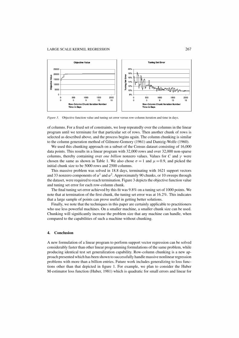
Figure 3. Objective function value and tuning set error versus row-column iteration and time in days.

of columns. For a fixed set of constraints, we loop repeatedly over the columns in the linearprogram until we terminate for that particular set of rows. Then another chunk of rows isselected as described above, and the process begins again. The column chunking is similarto the column generation method of Gilmore-Gomory (1961) and Dantzig-Wolfe (1960).

We used this chunking approach on a subset of the Census dataset consisting of 16,000data points. This results in a linear program with 32,000 rows and over 32,000 non-sparsecolumns, thereby containing over one billion nonzero values. Values for C and γ werechosen the same as shown in Table 1. We also chose σ = 1 and µ = 0.9, and picked theinitial chunk size to be 5000 rows and 2500 columns.

This massive problem was solved in 18.8 days, terminating with 1621 support vectorsand 33 nonzero components of α1 and α2. Approximately 90 chunks, or 10 sweeps throughthe dataset, were required to reach termination. Figure 3 depicts the objective function valueand tuning set error for each row-column chunk.

The final tuning set error achieved by this fit was 9.8% on a tuning set of 1000 points. Wenote that at termination of the first chunk, the tuning set error was at 16.2%. This indicatesthat a large sample of points can prove useful in getting better solutions.

Finally, we note that the techniques in this paper are certainly applicable to practitionerswho use less powerful machines. On a smaller machine, a smaller chunk size can be used.Chunking will significantly increase the problem size that any machine can handle, whencompared to the capabilities of such a machine without chunking.

4. Conclusion

A new formulation of a linear program to perform support vector regression can be solvedconsiderably faster than other linear programming formulations of the same problem, whileproducing identical test set generalization capability. Row-column chunking is a new ap-proach presented which has been shown to successfully handle massive nonlinear regressionproblems with more than a billion entries. Future work includes generalizing to loss func-tions other than that depicted in figure 1. For example, we plan to consider the HuberM-estimator loss function (Huber, 1981) which is quadratic for small errors and linear for


large errors by using quadratic programming. Extension to larger problems will also beconsidered using parallel processing for both linear and quadratic programming formula-tions.

Acknowledgments

The research described in this Data Mining Institute Report 99-02, August 1999, wassupported by National Science Foundation Grants CCR-9729842 and CDA-9623632, byAir Force Office of Scientific Research Grant F49620-97-1-0326 and by the MicrosoftCorporation.

References

Bennett, K. P. (1999). Combining support vector and mathematical programming methods for induction. In B.Scholkopf, C. Burges, & A. Smola (Eds.). Advances in kernel methods: Support vector mechines (pp. 307–326).Cambridge, MA: MIT Press.

Bradley, P. S. & Mangasarian, O. L. (2000). Massive data discrimination via linear support vector machines.Optimization, Methods and Software, (vol. 13, pp. 1–10). ftp://ftp.cs.wisc.edu/math-prog/tech-reports/98-03.ps

Burges, C. J. C. (1998). A tutorial on support vector machines for pattern recognition. Data Mining and KnowledgeDiscovery, 2:2, 121–167.

Cherkassky, V. & Mulier, F. (1998). Learning from data—concepts, theory and methods. New York: John Wiley& Sons.

Cortes, C. & Vapnik, V. (1995). Support vector networks. Machine Learning, 20, 273–279.Dantzig, G. B. & Wolfe, P. (1960). Decomposition principle for linear programs. Operations Research, 8, 101–111.Delve. Data for evaluating learning in valid experiments. http://www.cs.utoronto.ca/∼delve/Gilmore, P. C. & Gomory, R. E. (1961). A linear programming approach to the cutting stock problem. Operations

Research, 9, 849–859.Huber, P. J. (1964). Robust estimation of location parameter. Annals of Mathematical Statistics, 35, 73–101.Huber, P. J. (1981). Robust statistics. New York: John Wiley.ILOG CPLEX Division, Incline Village, Nevada. (1991). ILOG CPLEX 6.5 Reference Manual. 2000.Mangasarian, O. L. (2000). Generalized support vector machines. In A. Smola, P. Bartlett, B. Scholkopf, &

D. Schuurmans (Eds.). Advances in large margin classifiers (pp. 135–146). Cambridge, MA: MIT Press.ftp://ftp.cs.wisc.edu/math-prog/tech-reports/98-14.ps

Mangasarian, O. L. & Meyer, R. R. (1979). Nonlinear perturbation of linear programs. SIAM Journal on Controland Optimization, 17:6, 745–752.

MATLAB. (1994–2000). User’s guide. The MathWorks, Inc., Natick, MA 01760. http:/www.mathworks.com/products/matlab/usersguide.shtml

MATLAB. (1997). Application program interface guide. The MathWorks, Inc., Natick, MA 01760.Murphy, P. M. & Aha, D. W. (1992). UCI repository of machine learning databases. www.ics.uci.edu/∼mlearn/

MLRepository.htmlScholkopf, B., Bartlett, P., Smola, A., & Williamson, R. (1998). Support vector regression with automatic ac-

curacy control. In L. Niklasson, M. Boden, & T. Ziemke (Eds.). Proceedings of the Eight International Con-ference on Artificial Neural Networks (pp. 111–116) Berlin: Springer Verlag. Available at http://www.kernel-machines.org/publications.html

Scholkopf, B., Bartlett, P., Smola, A., & Williamson, R. (1999). Shrinking the tube: A new support vector re-gression algorithm. In M. S. Kearns, S. A. Solla, & D. A. Cohn (Eds.). Advances in neural informationprocessing systems (vol. 11, pp. 330–336). Cambridge, MA: MIT Press. Available at http://www.kernel-machines.org/publications.html

Scholkopf, B., Burges, C., & Smola, A. (Eds.). (1999). Advances in kernel methods: Support vector machines.Cambridge, MA: MIT Press.


Smola, A. J. (1998). Learning with kernels. Ph.D. Thesis, Technische Universitat Berlin, Berlin, Germany.Smola, A., Scholkopf, B., & Ratsch, G. (1999). Linear programs for automatic accuracy control in regression. In

Ninth International Conference on Artificial Neural Networks, Conference Publications No. 470 (pp. 575–580).London: IEE. Available at http://www.kernel-machines.org/publications.html

Street, W. N. & Mangasarian, O. L. (1998). Improved generalization via tolerant training. Journal of OptimizationTheory and Applications, 96:2, 259–279. ftp://ftp.cs.wisc.edu/math-prog/tech-reports/95-11.ps

US Census Bureau. Adult dataset. Publicly available from www.sgi.com/Technology/mlc/db/.Vapnik, V. N. (1995). The nature of statistical learning theory. New York: Springer.Weston, J., Gammerman, A., Stitson, M., Vapnik, V., Vovk, V., & Watkins, C. (1997). Support vector density

estimation. In B. Scholkopf, C. Burnes, & A. Smola (Eds.). Advances in kernel methods: Support vectormachines (pp. 293–306). Cambridge, MA: MIT Press.

Received February 1, 2000Revised March 1, 2001Accepted March 1, 2001Final manuscript March 1, 2001

Documents

Large Scale Kernel Regression via Linear Programming