Laplacian Mixture Modeling for Overcomplete Mixing Matrix in Wavelet Packet … · 2006-09-30 · Packet Domain by Adaptive EM-type Algorithm and Comparisons ... mixtures of speech

1

Laplacian Mixture Modeling for Overcomplete Mixing Matrix in Wavelet Packet Domain by Adaptive EM-type Algorithm and Comparisons

Behzad Mozaffary Mohammad A. Tinati

Faculty of Electrical and Computer Engineering Univercity of Tabriz

29 Bahman Blvd., Tabriz, East Azerbaijan IRAN

Abstract-- Speech process has benefited a great deal from the wavelet transforms. Wavelet packets decompose signals in to broader components using linear spectral bisecting. In this paper, mixtures of speech signals are decomposed using wavelet packets, the phase difference between the two mixtures are investigated in wavelet domain. In our method Laplacian Mixture Model (LMM) is defined. An Expectation Maximization (EM) algorithm is used for training of the model and calculation of model parameters which is the mixture matrix. And then we compare estimation of mixing matrix by LMM-EM with different wavelet. Therefore individual speech components of speech mixtures are separated.

Keywords: ICA, Laplacian Mixture Model, Expectation Maximization, wavelet packets, Blind Source Separation, Speech Processing

1. Introduction

Blind source separation techniques using independent component analysis (ICA) have many potential applications including speech recognition systems, telecommunications, and biomedical signal processing. The goal of ICA is to recover independent sources given only sensor observation datum that are unknown linear mixtures of the unobserved independent source signals [1]–[6]. The standard formulation of ICA requires at least as many sensors as sources.

Lewicki and Sejnowski [7], [8] have proposed a generalized ICA method for learning overcomplete representations of data that allows more basis vectors than dimensions in the input. Several approaches have been investigated to address the overcomplete source separation problems in the past. Lewicki [9] provided a complete Baysian approach assuming Laplacian source prior to estimating both the mixing matrix and the source in the time domain. Clustering solutions were introduced by Hyvarinen [10] and Bofill-Zibulesky [11]. Davies and Miltianoudis [12] employed modified discrete cosine transform (MDCT) to obtain a sparse representation. They proposed a two-state Gassian mixture model (GMM) to represent the source densities and the possible

additive noise and used an expectation-maximization, (EM)-type algorithm, to perform separation with reasonable performance.

In this paper, we explore the case of two-sensor setup with no additive noise, where the source separation problem becomes a one-dimensional optimal detection problem. The phase difference between the two-sensor data is employed. A Laplacian mixture model (LMM) is fitted to the phase difference between the two sensors, using an EM-type algorithm in each wavelet packet. The LMM model can be used for source separation and source localization. Since in the overcomplete model of source separation estimation of mixture matrix is very important in this paper, therefore we use LMM model for each wavelet packet with phase differences. Note that wavelet packets are obtained from decomposition of two mixtures.

2. Background Material

Wavelets are transform methods that has received

great deal of attention over the past several years. The wavelet transform is a time-scale representation method that decomposes signals into basis functions of time and scale, which makes it useful in

Proceedings of the 5th WSEAS International Conference on Signal Processing, Istanbul, Turkey, May 27-29, 2006 (pp145-150)

2

applications such as signal denoising, wave detection, data compression, feature extraction, etc.

There are many techniques based on wavelet theory, such as wavelet packets, wavelet approximation and decomposition, discrete and continuous wavelet transform, etc.

Backbone of the wavelets theory is the following two equations:

)2(2)( 2/, ktt jjkj −= φφ (1)

)2(2)( 2/, ktt jjkj −= ψψ (2)

Where )(tφ and )(tψ are basic scaling function and mother wavelet function respectively.

The wavelet system is a set of building blocks to construct or represent a signal or function. It is a two dimensional expansion set. A linear expansion would be:

,0

( ) ( ) (2 )jk j k

k k j

f t c t k d t kϕ ψ+∞ +∞ +∞

=−∞ =−∞ =

= − + −∑ ∑∑ (3)

Most of the results of wavelet theory are developed

using filter banks. In applications one never has to deal directly with the scaling functions or wavelets, only the coefficients of the filters in the filter banks are needed 0. A full wavelet packet decomposition binary tree for tree scale wavelet packet transform is shown in figure (1).

Figure (1)

3. Mathematical Model

Assume a set of M sensors expressed as a vector: T

M txtxtxtxtX )](...,)(,)(,)([)( 321= where xi(t) is the output of the ith sensor and also assume that there are N source signals as in vector:

TN tststststS )](...,)(,)(,)([)( 321=

where again si(t) is the ith source. In this paper we will assume noise-less instantaneous mixing model i.e. )(.)( tSAtX = Where A denotes the mixing matrix. The source separation problems consist of estimating the original sources )(tS , given the observed signals )(tX . In the case of an equal number of sources and sensors (N=M), a number of robust approaches using independent component analysis (ICA) have been proposed by Mitianoudis [14]. In the overcomplete source separation case (M<N), the source separation problem consists of two sub problems i) estimating the mixing matrix A and ii) estimating the source signals )(tS .

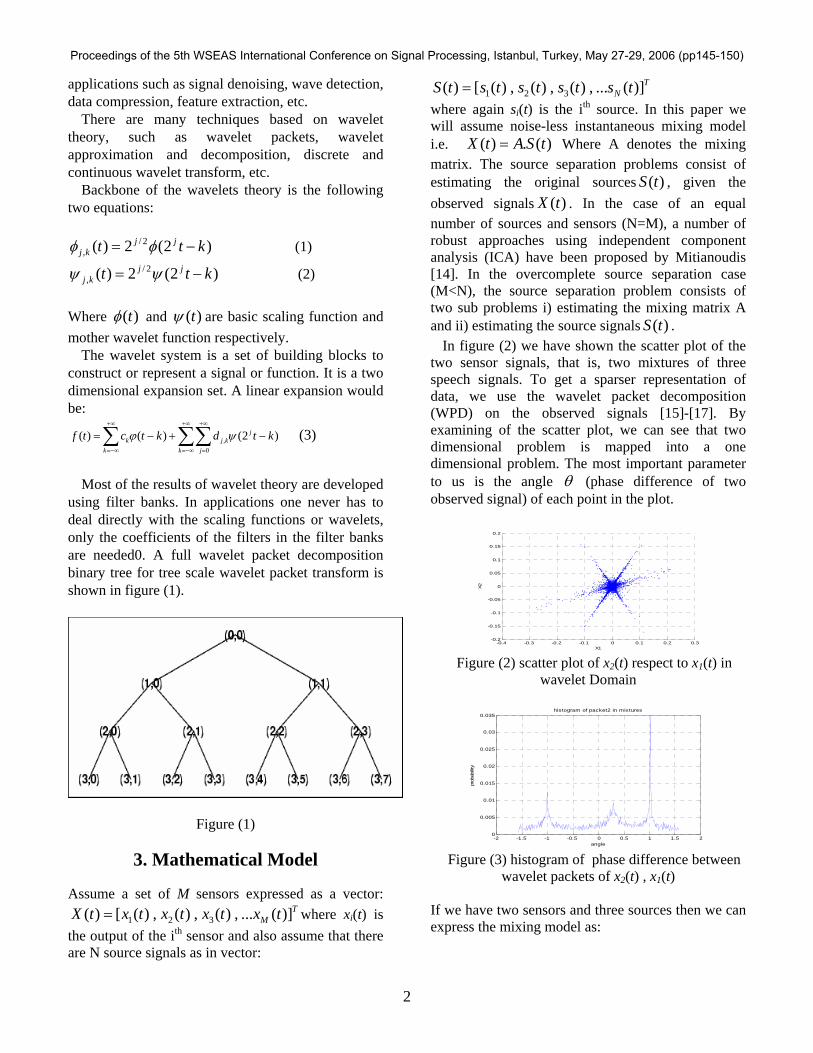
In figure (2) we have shown the scatter plot of the two sensor signals, that is, two mixtures of three speech signals. To get a sparser representation of data, we use the wavelet packet decomposition (WPD) on the observed signals [15]-[17]. By examining of the scatter plot, we can see that two dimensional problem is mapped into a one dimensional problem. The most important parameter to us is the angle θ (phase difference of two observed signal) of each point in the plot.

-0.4 -0.3 -0.2 -0.1 0 0.1 0.2 0.3-0.2

-0.15

-0.1

-0.05

0

0.05

0.1

0.15

0.2

X1

X2

Figure (2) scatter plot of x2(t) respect to x1(t) in

wavelet Domain

-2 -1.5 -1 -0.5 0 0.5 1 1.5 20

0.005

0.01

0.015

0.02

0.025

0.03

0.035histogram of packet2 in mixtures

angle

prob

ability

Figure (3) histogram of phase difference between

wavelet packets of x2(t) , x1(t) If we have two sensors and three sources then we can express the mixing model as:


3

⎩⎨⎧

++=++=

)()()()()()()()(

3232221212

3132121111

tsatsatsatxtsatsatsatx

(4)

ASX = (5) For simplicity we assume 1 1ja = for all j=1 ,2 ,3 and then we can write :

332211)( sbsbsbtX ++= (6) Equation (6) indicates that each source signal in the scatter plots will be in the jb direction.

We define phase difference of observed data measured by sensors as follows:

])()([

1

2

xPxParctg

i

it =θ (7)

Where Pi(xj) is the ith packet wavelet of jth observation signal. In figure (3) we have plotted the histogram of the phase difference of observed signals in wavelet packet domain.

4.Laplacian Mixture Modeling

The laplacian density is usually expressed as: 0),,( 0

θθθθ −−= ccecL (8) Where 0θ represent the center of density function and c>0 controls the width or variance of the density. An LMM is defined as:

∑∑=

−−

=

==N

k

ckk

N

kkkk

keccLf11

),,()( θθαθθαθ (9)

Where kkk c,,θα are the weights, centers, and widths of each Laplacian respectively. In the next section we will show how the EM algorithm is used to train the model to get the optimum values of the model parameters.

5. Training Process Using the EM Algorithm

In [18] Bilmes proposed a procedure to find

maximum likelihood mixture (MLM) density parameters using EM. In this section, we use the EM algorithm to train a LMM, based on [18]. Assuming T samples for kθ and Laplacian mixture densities as in equation (8), the log likelihood takes the following form:

∑∑

∑ ∑

= =

= =

−−+=

=

T

t

N

ktktkkk

T

t

N

kkktkkkk

kfcc

cLcJ

1 1

1 1

)()2log(log

),,(log),,(

θθθα

θθαθα (10)

Where )( tkf θ represents the probability of tθ belonging to kth Laplacian distribution. The iteration rules update )( tkf θ and kα .

To obtain the update values for kt c,θ we solved derivatives of ),,( kkk cJ θα with respect to kt c,θ , that is:

0 ,0 =∂∂

=∂∂

kk cJJ

θ (11)

Using these iteration formulas we are able to train

the LMM and estimate the center and other parameters of each Laplacian distribution. The block diagram of the proposed algrith is shown in figure (4).

Figure (4)

As the figure (4) shows, the wavelet packets of the

two mixtures of speech signal, x1(t) and x2(t), is obtained. Then in every filter bank, the phase differences of the packets of x1(t) and x2(t) is calculated. The next step is to manipulate the histograms of the phase angle differences. The center

Obtaining Mixtures of X2(t) , X1(t)

Wavelet Packet Decomposition for each mixtures

Obtaining Phase differences between packets

Calculation of Pahse differences Histogram

LMM-EM

Calculation of mixiture matrix


4

of each Laplacian density is estimated using the Laplacian mixture model. The training algorithm used in this process is an EM type. Therefore, after the convergence of the EM, the estimation of the mixture matrix is obtained.

6. Experiment and simulation

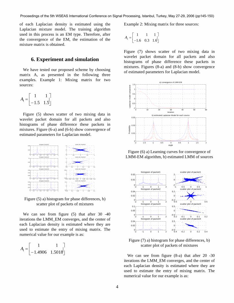
We have tested our proposed scheme by choosing matrix A, as presented in the following three examples. Example 1: Mixing matrix for two sources:

⎥⎦

⎤⎢⎣

⎡−

=5.15.1

111A

Figure (5) shows scatter of two mixing data in

wavelet packet domain for all packets and also histograms of phase difference these packets in mixtures. Figure (6-a) and (6-b) show convergence of estimated parameters for Laplacian model.

-2 -1.5 -1 -0.5 0 0.5 1 1.5 20

0.02

0.04histogram of packet1

-1 -0.5 0 0.5 1-2

0

2scatter plot of packet1

-2 -1.5 -1 -0.5 0 0.5 1 1.5 20

0.05


-0.4 -0.2 0 0.2 0.4 0.6-1

0


-2 -1.5 -1 -0.5 0 0.5 1 1.5 20

0.02

0.04


-0.02 -0.015 -0.01 -0.005 0 0.005 0.01 0.015 0.02-0.05

0

0.05scatter plot of packet3

-2 -1.5 -1 -0.5 0 0.5 1 1.5 20

0.01

0.02


-0.15 -0.1 -0.05 0 0.05 0.1-0.2

0


Figure (5) a) histogram for phase differences, b)

scatter plot of packets of mixtures

We can see from figure (5) that after 30 -40 iterations the LMM_EM converges, and the center of each Laplacian density is estimated where they are used to estimate the entry of mixing matrix. The numerical value for our example is as:

⎥⎦

⎤⎢⎣

⎡−

=5018.14906.111

1A

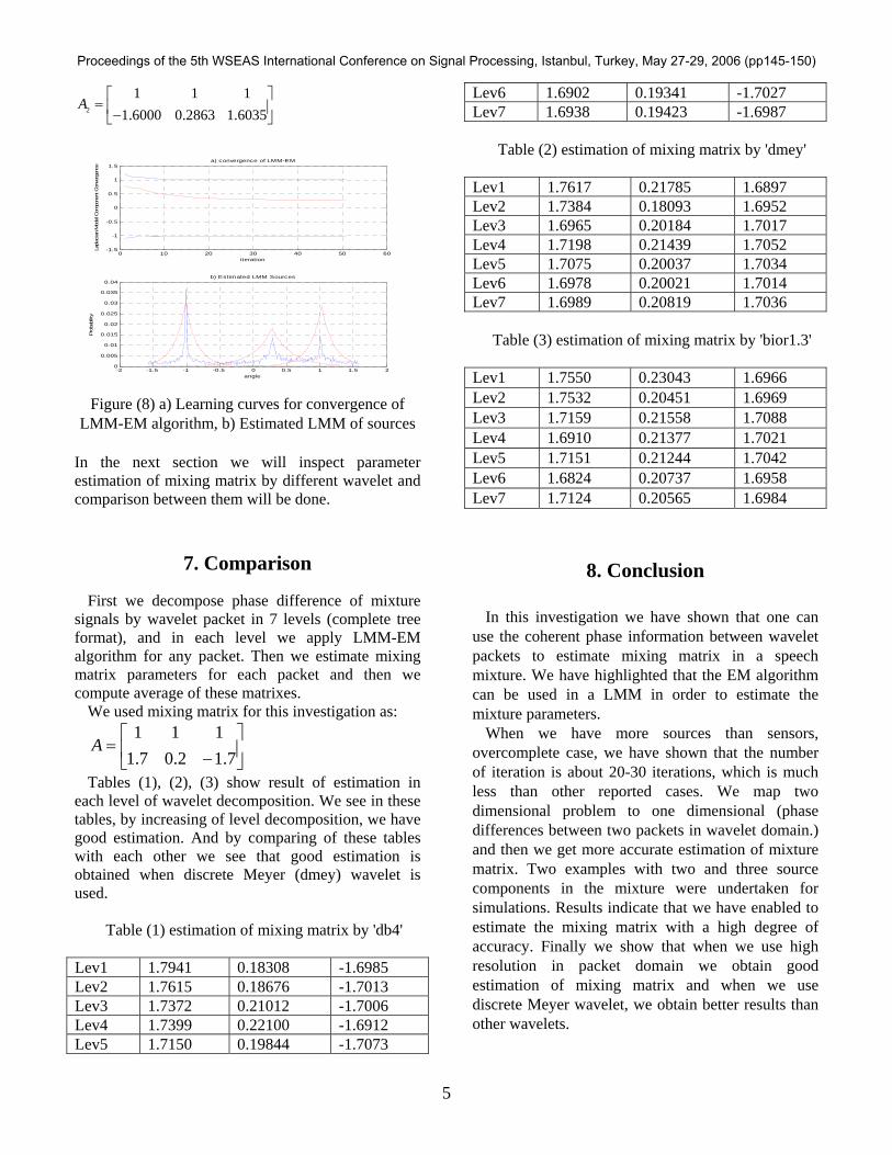
Example 2: Mixing matrix for three sources:

2

1 1 11.6 0.3 1.6

A⎡ ⎤

= ⎢ ⎥−⎣ ⎦

Figure (7) shows scatter of two mixing data in wavelet packet domain for all packets and also histograms of phase difference these packets in mixtures. Figures (8-a) and (8-b) show convergence of estimated parameters for Laplacian model.

0 10 20 30 40 50 60-1

-0.5

0

0.5

1

1.5a) convergence of LMM-EM

iteration

Lapl

acia

n m

odel

com

pone

nt

-2 -1.5 -1 -0.5 0 0.5 1 1.5 20

0.01

0.02

0.03b) estimated Laplasian Model for each source

angle

Pro

babi

lity

Figure (6) a) Learning curves for convergence of

LMM-EM algorithm, b) estimated LMM of sources

-2 -1 0 1 20

0.01


-1 -0.5 0 0.5 1-2

0


-2 -1 0 1 20

0.02


-0.5 0 0.5-0.2

0


-2 -1 0 1 20

0.05


-0.2 -0.1 0 0.1 0.2-0.5

0


-2 -1 0 1 20

0.02


-0.4 -0.2 0 0.2 0.4-0.5

0


Figure (7) a) histogram for phase differences, b)

scatter plot of packets of mixtures

We can see from figure (8-a) that after 20 -30 iterations the LMM_EM converges, and the center of each Laplacian density is estimated where they are used to estimate the entry of mixing matrix. The numerical value for our example is as:


5

2

1 1 11.6000 0.2863 1.6035

A ⎡ ⎤= ⎢ ⎥−⎣ ⎦

0 10 20 30 40 50 60-1.5

-1

-0.5

0

0.5

1

1.5a) convergence of LMM-EM

iteration

Laplac

ian

Mod

el C

ompo

nent

Con

verg

ence

-2 -1.5 -1 -0.5 0 0.5 1 1.5 20

0.005

0.01

0.015

0.02

0.025

0.03

0.035

0.04b) Estimated LMM Sources

angle

Pro

bability

Figure (8) a) Learning curves for convergence of

LMM-EM algorithm, b) Estimated LMM of sources In the next section we will inspect parameter estimation of mixing matrix by different wavelet and comparison between them will be done.

7. Comparison

First we decompose phase difference of mixture

signals by wavelet packet in 7 levels (complete tree format), and in each level we apply LMM-EM algorithm for any packet. Then we estimate mixing matrix parameters for each packet and then we compute average of these matrixes.

We used mixing matrix for this investigation as:

⎥⎦

⎤⎢⎣

⎡−

=7.12.07.1

111A

Tables (1), (2), (3) show result of estimation in each level of wavelet decomposition. We see in these tables, by increasing of level decomposition, we have good estimation. And by comparing of these tables with each other we see that good estimation is obtained when discrete Meyer (dmey) wavelet is used.

Table (1) estimation of mixing matrix by 'db4'

Lev1 1.7941 0.18308 -1.6985 Lev2 1.7615 0.18676 -1.7013 Lev3 1.7372 0.21012 -1.7006 Lev4 1.7399 0.22100 -1.6912 Lev5 1.7150 0.19844 -1.7073

Lev6 1.6902 0.19341 -1.7027 Lev7 1.6938 0.19423 -1.6987

Table (2) estimation of mixing matrix by 'dmey'

Lev1 1.7617 0.21785 1.6897 Lev2 1.7384 0.18093 1.6952 Lev3 1.6965 0.20184 1.7017 Lev4 1.7198 0.21439 1.7052 Lev5 1.7075 0.20037 1.7034 Lev6 1.6978 0.20021 1.7014 Lev7 1.6989 0.20819 1.7036

Table (3) estimation of mixing matrix by 'bior1.3'

Lev1 1.7550 0.23043 1.6966 Lev2 1.7532 0.20451 1.6969 Lev3 1.7159 0.21558 1.7088 Lev4 1.6910 0.21377 1.7021 Lev5 1.7151 0.21244 1.7042 Lev6 1.6824 0.20737 1.6958 Lev7 1.7124 0.20565 1.6984

8. Conclusion

In this investigation we have shown that one can use the coherent phase information between wavelet packets to estimate mixing matrix in a speech mixture. We have highlighted that the EM algorithm can be used in a LMM in order to estimate the mixture parameters.

When we have more sources than sensors, overcomplete case, we have shown that the number of iteration is about 20-30 iterations, which is much less than other reported cases. We map two dimensional problem to one dimensional (phase differences between two packets in wavelet domain.) and then we get more accurate estimation of mixture matrix. Two examples with two and three source components in the mixture were undertaken for simulations. Results indicate that we have enabled to estimate the mixing matrix with a high degree of accuracy. Finally we show that when we use high resolution in packet domain we obtain good estimation of mixing matrix and when we use discrete Meyer wavelet, we obtain better results than other wavelets.


6

9. References

[1] A. J. Bell and T. J. Sejnowski, “An information-maximization approach to blind separation and blind deconvolution,” Neural Comput., vol. 7, pp. 1129–1159, 1995. [2] J.-F. Cardoso, “Blind signal separation: Statistical principles,” Proc. IEEE, vol. 86, pp. 2009–2025, Oct. 1998. [3] P. Comon, “Independent component analysis—A new concept?,” Signal Process., vol. 36, pp. 287–314, 1994. [4] P. Comon and B. Mourrain, “Decomposition of quantics in sums of powers of linear forms,” Signal Process., vol. 53, pp. 93–107, Sept. 1996. [5] M. Hermann and H. Yang, “Perspectives and limitations of selforganizing maps,” in Proc. ICONIP’96. [6] T.-W. Lee, Independent Component Analysis: Theory and Applications. Boston, MA: Kluwer, 1998. [7] M. Lewicki and T. J. Sejnowski, “Learning nonlinear overcomplete representations for efficient coding,” in Advances in Neural Information Processing Systems, vol. 10. Cambridge, MA: MIT Press, 1998, pp. 815–821. [8] M. S. Lewicki and T. J. Sejnowski, “Learning over complete representations,” Neural Comput., to be published. [9] M. Lewicki and T.J. Sejnowski, "Learning over complete representations networks," Neural Compute., vol. 12,pp.337-365,2000 [10] A. Hyvarinen, "Independent component analysis in the presence of Gassian noise by maximizing joint likelihood networks," Neural Compute., vol. 22, pp.49-67,1998\ [11] P. Bofill and M. Zibulevsky, "Underdetermined blind source separation using sparce representation networks," Signal Process., vol. 81, no. 11, pp. 2353-2362, 2001

[12] M. Davies and N. Mitianoudis, "A simple mixture model for sparce overcomplete ICA networks," Proc. Inst. Elec. Eng. Vision, Image,Signal Process., vol. 151, no. 1, pp. 35-43 , 2004. [13] C. S. Burrus, R. A. Gopinath, H. Guo, “Introduction to Wavelets and Wavelet Transforms, a primer” Prentice Hall New jersey, 1998. [14] N. Mitianoudis, "Audio source separation using independent component analysis," Ph.D. dissertation, Queen Mary, London, U.K, 2004 [15] M.A. Tinati, B. Mozaffari, “Comparison of Time-frequency and Time-scale analysis of speech signals using STFT and DWT, ” WSEAS Transaction on Signal Processing, Issue 1, Vol. 1, pp. 11-16, Oct. 2005 [16] M.A. Tinati, B. Mozaffari, “A Novel Method for Noise Cancellation of Speech Signals Using Wavelet Packets” [17] M. Zibulevsky, P. Kisilev, Y. Y. Zeevi, and B. A. Pearlmutter, "Blind source separation via multimode sparse representation networks, " Adv. Neural Inf. Process. Syst., vol. 14, pp. 1049-1056, 2002 [18] J. A. Bilmes, "A Gentle Tutorial of the EM Algorithm and it's application to parameter estimation for Gassian Mixtures and Hidden Mixture Models, " Dept. Elect. Eng. Comput. Sci. , Univ. California, Berkeley, California, Tech. Rep. , 1998.


Documents

Laplacian Mixture Modeling for Overcomplete Mixing Matrix in Wavelet Packet … · 2006-09-30 · Packet Domain by Adaptive EM-type Algorithm and Comparisons ... mixtures of speech