Image Denoising by Modified Overcomplete Wavelet ... · Image Denoising by Modified Overcomplete Wavelet Representation Utilizing Adaptive Thresholding Algorithm Jitha C R Abstract—

International Journal of Scientific & Engineering Research, Volume 6, Issue 4, April-2015 ISSN 2229-5518

IJSER © 2015

http://www.ijser.org

Image Denoising by Modified Overcomplete Wavelet Representation Utilizing Adaptive

Thresholding Algorithm Jitha C R

Abstract— For images corrupted with Gaussian noise, the wavelet thresholding proves to be an effective approach to remove as much

noise while retaining important signal features, but the performance decreases under heavy noise because the amount of noise is not

considerd while denoising. This paper aims at implementing an efficient image denoising method adaptive to the noise and is achieved by

using an adaptive wavelet packet thresholding function based on a modified form of overcomplete wavelet representation. The adaptive

algorithm is called OLI – Shrink and certain changes have been applied to the original form of overcomplete representation so that it

become perfectly compatible for the application of OLI-Shrink. The performance of the algorithm is evaluated by computing the Peak

Signal to Noise Ratio (PSNR) and a new performance measure called the Universal Image Quality Index (UIQI) and is found to outperform

various existing wavelet based denoising algorithms.

Index Terms— Adaptive thresholding algorithm, coefficient thresholding, image denoising, optimal wavelet basis (OWB), over-complete

representation, subband weighting function, wavelet packet transform.

—————————— ——————————

1 INTRODUCTION

isual information transmitted in the form of d igital images

is becoming a major method of communication in the

modern age, but is often corrupted with noise either in its

acquisition or transmission . The goal of denoising is to remove

the noise while retaining as much as possible the important

signal features such as edges, textures etc. The wavelet based

approach is the best option for denoising images corrupted

with Gaussian noise. In wavelet domain, noise is uniformly

spread throughout the coefficients while most of the image

information is concentrated in the few largest ones. This idea

is the basis of denoising by means of coefficient thresholding.

Conventional methods do not take the intensity of noise in-

to consideration and is therefore operating in a similar manner

to images containing noise at d ifferent levels. So a new me-

thod is to be designed such that as the noise con tent varies, the

value of threshold must also change and the denoising algo-

rithm must be adap tive to noise. In other words, the denoising

should be based on an adaptive thresholding function . This

paper aims at implementing such an efficient image denoising

method based on a new adaptive wavelet packet thresholding

function. The new technique called Optimum Linear Interpo-

lation Shrink or OLI-Shrink algorithm is a wavelet based

adaptive thresholding algorithm and operates on the image on

the basis of the estimated noise and is hence an adaptive tech-

nique. The new value an optimum value found using MAP

based estimation ru les incorporating the data mean, noise v a-

riance, and certain weighting constants depend ing on both

data and noise parameters. The overall denoising achieved by

applying the OLI-Shrink method as part of the overcomplete

wavelet (OCW) representation. Overcomplete wavelet repre-

sentation improve SNR of simple DWT based methods by av-

eraging the results obtained via separate independent m e-

thods.

A high quality image is taken and some known noise

is added to it. This would then be given as input to the denois-

ing section, which produces an image close to the original high

quality image. The performance of most of the algorithms are

evaluated by computing the Peak Signal to Noise Ratio

(PSNR) but this does not give any implication on the per-

ceived quality. So a new image quality index introduced to

compare images based on their visual quality which is known

as the Universal Image Quality Index (UIQI).

2 BASIC WAVELET DENOISING

The concept of wavelets was introduced in 1984 for analysing

the information content of images. Later, Stephane G. Mallat

introduced a theoretical foundation for multiresolu tion signal

decomposition which is technically termed as the wavelet re-

presentation. Wavelets are mathematical functions that cut up

data into d ifferent frequency components and then study each

component with a resolu tion matched to its size. The analysis

involves adopting a prototype wavelet function called mother

wavelet. Wavelet systems are generated from single scaling

function by scaling and translation. The original signal can be

represented in terms of wavelets using the coefficients in a

linear combination format. They are advantageous over the

traditional Fourier methods in analysing signals that contain

d iscontinuities and sharp sp ikes. Wavelet transform generates

sequence of signals known as approximation signals with d e-

creasing resolu tion supplemented by a sequence of additional

touches called details.

V

————————————————

Jitha C. R. has received Bachelor of Technology in Electronics and Communi-

cation Engineering from Mahatma Gandhi University, Kerala, India in 2012

and Master of Technology in Communication Engineering from Mahatma

Gandhi University, Kerala, India in 2014.

802

IJSER


IJSER © 2015


Wavelets help to remove noise through the technique

called wavelet shrinkage or thresholding methods. When a

signal is decomposed using wavelet, the resultant is a set of

data called the wavelet coefficients. Some of them contain the

majority of signal data while others correspond to details. If

the details are small, they might be omitted without substan-

tially affecting the main features of interest. If the coefficients

below a certain threshold are truncated the data is sparsely

represented and this sparse coding makes wavelets an excel-

lent tool in data compression and removing noise. So the idea

of thresholding is to set to zero all coefficients that are less

than a particular threshold . These coefficients are used in an

inverse wavelet transformation to reconstruct the data set.

Wavelet denoising involves three steps:

1) A linear forward wavelet transform

2) Non-linear thresholding

3) A linear inverse wavelet transform

Thresholding is a non-linear technique which operates on

one wavelet coefficient at a time. The smaller coefficients are

more likely due to noise and large coefficients due to impor-

tant signal features. Hence thresholding smaller ones help to

avoid noise. Each coefficient is thresholded by comparing

against a threshold . To remove noise, the choice of threshold is

extremely important. It shou ld not be too small or too large. If

the threshold value is too small, most of the noise remains

whereas a large threshold fails to preserve image features.

Hence an optimum value is essential. Wavelet shrinkage d e-

pends heavily on the choice of thresholding parameter and the

nature of the thresholding function .

3 EXISTING METHODS

Denoising via wavelet packet (WP) base w as introduced in

2007. Unlike wavelet transform, the wavelet packet transform

(WPT) decomposes both approximation and detail subbands.

Thus the resulting wavelet packet decomposition consists of

more subbands than corresponding wavelet decomposition.

At every decomposition level, all the subbands are subd i-

vided. The main advantage of such a decomposition is that a

minimal representation can be obtained by suitably choosing

which subbands to split and thus a choice can be made be-

tween several possible combinations of subbands.

A prominent denoising method was introduced by G.

Deng, D. B. H. Tay, and S. Marusic which was based on over-

complete wavelet representation and Gaussian models [2]. The

method uses a signal estimation technique based on multiple

wavelet representations called the overcomplete representa-

tion. But no algorithm was specified to achieve the expected

result. Also, WPT was not used . A denoising algorithm using

WPT with a new type of thresholding is the optimum linear

interpolation method put forward by Abdolhossein Fathi and

Ahmad Reza Naghsh Nilchi [1].

4 PROPOSED METHOD

Overcomplete wavelet representation uses two or more similar

wavelets to denoise a noisy image. Here, the pairs of wavelets

used are either similar in properties or originate from a single

wavelet by means of double shifting or reversing. Some pairs

used include sym12 and coif4, sym4 and db4, sym12 and

sym12d, coif4 and coif4d , sym12 and sym12r, coif4 and coif4r . A modified form of the conventional over-complete re-

presentation is used here. Instead of WT for signal decomposi-

tion, WPT is used and then optimal wavelet basis (OWB) is

found. Another d ifference is that the Walsh Hadamard Tran s-

form (WHT) and the inverse WHT are not used . Also the forward transforms involve conditional decom-

position of the input image using selected wavelet pairs. The

coefficients thus obtained are the noisy coeffients and so a

MAP denoising algorithm is applied which estimates the

noise. The algorithm is based on an adaptive thresholding

function. Then an optimum interpolation function is used in

the thresholding step which more effective than the conven-

tional hard or soft thresholding ru les. After modifying each

and every coefficient present, a new set of coefficients is ob-

tained. Finally, this undergo inverse WPT and and is averaged.

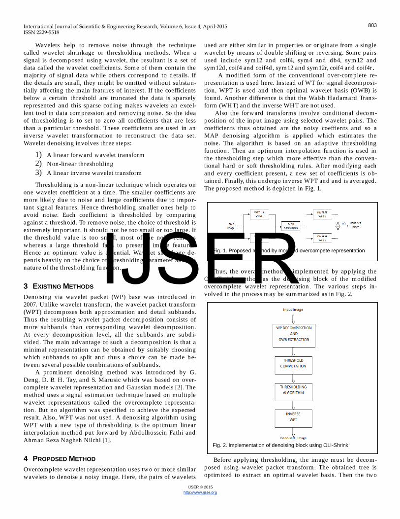
The proposed method is depicted in Fig. 1.

Thus, the overall method is implemented by applying the

OLI-Shrink method as the denoising block of the modified

overcomplete wavelet representation . The various steps in-

volved in the process may be summarized as in Fig. 2.

Before applying thresholding, the image must be decom-

posed using wavelet packet transform. The obtained tree is

optimized to extract an optimal wavelet basis. Then the two

Fig. 1. Proposed method by modified overcompete representation

Fig. 2. Implementation of denoising block using OLI-Shrink

803

IJSER


IJSER © 2015


sets independently undergo MAP based denoising process

using the same denoising algorithm. Computation of the thre-

shold value and application of thresholding algorithm togeth-

er forms the denoising step. Denoised coefficients are con-

verted to spatial domain by inverse wavelet packet transform.

The denoised images can be averaged to get final outputs.

5 WAVELET PACKET AND THE OPTIMAL WAVELET BASIS

(OWB)

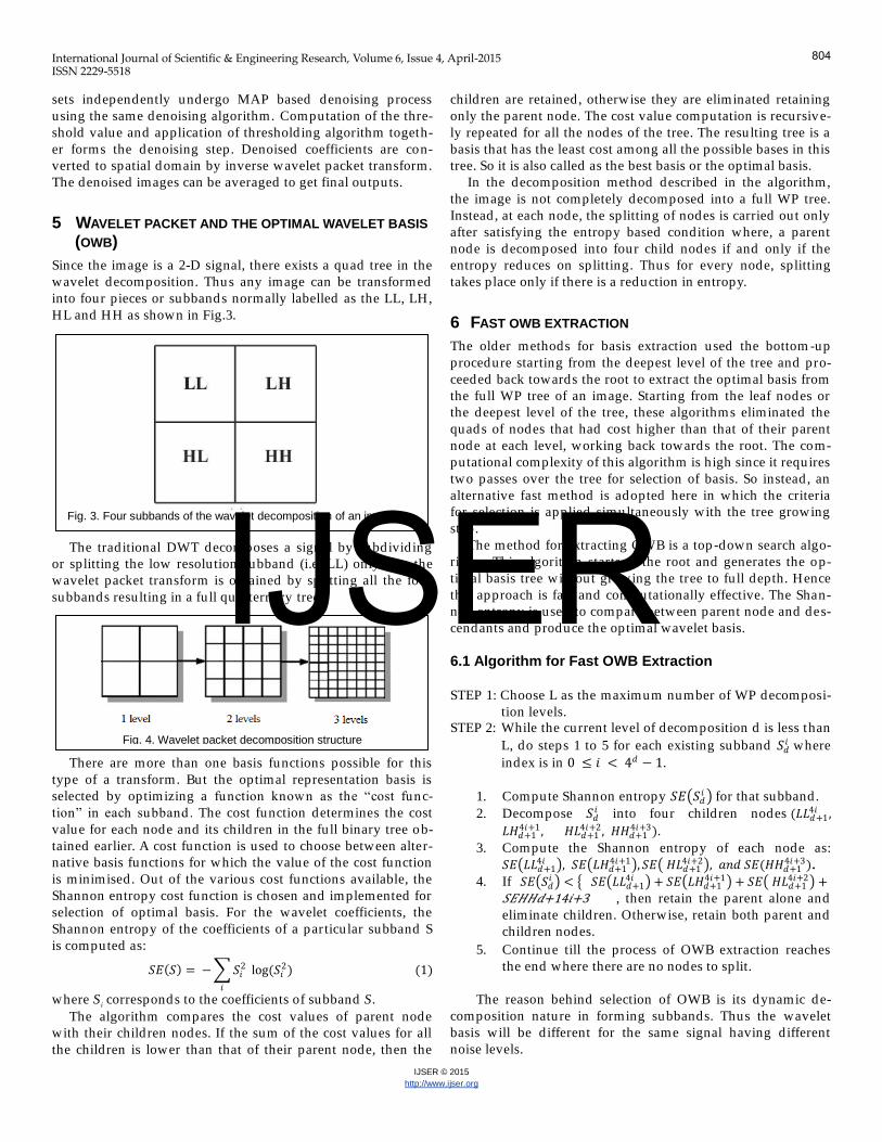
Since the image is a 2-D signal, there exists a quad tree in the

wavelet decomposition. Thus any image can be transformed

into four pieces or subbands normally labelled as the LL, LH,

HL and HH as shown in Fig.3.

The traditional DWT decomposes a signal by subdivid ing

or splitting the low resolu tion subband (i.e, LL) only. But the

wavelet packet transform is obtained by splitting all the four

subbands resulting in a fu ll quarternary tree.

There are more than one basis functions possible for this

type of a transform. But the optimal representation basis is

selected by optimizing a function known as the ―cost func-

tion‖ in each subband. The cost function determines the cost

value for each node and its children in the fu ll binary tree ob-

tained earlier. A cost function is used to choose between alter-

native basis functions for which the value of the cost function

is minimised . Out of the various cost functions available, the

Shannon entropy cost function is chosen and implemented for

selection of optimal basis. For the wavelet coefficients, the

Shannon entropy of the coefficients of a par ticular subband S

is computed as:

𝑆𝐸 𝑆 = − 𝑆𝑖2

𝑖

log(𝑆𝑖2) (1)

where Si corresponds to the coefficients of subband S.

The algorithm compares the cost values of parent node

with their children nodes. If the sum of the cost values for all

the children is lower than that of their parent node, then the

children are retained, otherwise they are eliminated retaining

only the parent node. The cost value computation is recursive-

ly repeated for all the nodes of the tree. The resulting tree is a

basis that has the least cost among all the possible bases in this

tree. So it is also called as the best basis or the optimal basis.

In the decomposition method described in the algorithm,

the image is not completely decomposed into a fu ll WP tree.

Instead , at each node, the splitting of nodes is carried out only

after satisfying the entropy based condition where, a parent

node is decomposed into four child nodes if and only if the

entropy reduces on splitting. Thus for every node, splitting

takes place only if there is a reduction in entropy.

6 FAST OWB EXTRACTION

The older methods for basis extraction used the bottom -up

procedure starting from the deepest level of the tree and pro-

ceeded back towards the root to extract the optimal basis from

the fu ll WP tree of an image. Starting from the leaf nodes or

the deepest level of the tree, these algorithms eliminated the

quads of nodes that had cost higher than that of their parent

node at each level, working back towards the root. The com-

putational complexity of this algorithm is high since it requires

two passes over the tree for selection of basis. So instead , an

alternative fast method is adopted here in which the criteria

for selection is applied simultaneously with the tree growing

step.

The method for extracting OWB is a top -down search algo-

rithm. This algorithm starts at the root and generates the op-

timal basis tree without growing the tree to fu ll depth. Hence

this approach is fast and computationally effective. The Shan-

non entropy is used to compare between parent node and des-

cendants and produce the optimal wavelet basis.

6.1 Algorithm for Fast OWB Extraction

STEP 1: Choose L as the maximum number of WP decomposi-

tion levels.

STEP 2: While the current level of decomposition d is less than

L, do steps 1 to 5 for each existing subband 𝑆𝑑𝑖 where

index is in 0 ≤ 𝑖 < 4𝑑 − 1.

1. Compute Shannon entropy 𝑆𝐸 𝑆𝑑𝑖 for that subband.

2. Decompose 𝑆𝑑𝑖 into four children nodes (𝐿𝐿𝑑+1

4𝑖 ,

𝐿𝐻𝑑+14𝑖+1 , 𝐻𝐿𝑑+1

4𝑖+2, 𝐻𝐻𝑑+14𝑖+3).

3. Compute the Shannon entropy of each node as:

𝑆𝐸 𝐿𝐿𝑑+14𝑖 , 𝑆𝐸 𝐿𝐻𝑑+1

4𝑖+1 ,𝑆𝐸 𝐻𝐿𝑑+14𝑖+2 , 𝑎𝑛𝑑 𝑆𝐸(𝐻𝐻𝑑+1

4𝑖+3). 4. If 𝑆𝐸 𝑆𝑑

𝑖 < 𝑆𝐸 𝐿𝐿𝑑+14𝑖 + 𝑆𝐸 𝐿𝐻𝑑+1

4𝑖+1 + 𝑆𝐸 𝐻𝐿𝑑+14𝑖+2 +

𝑆𝐸𝐻𝐻𝑑+14𝑖+3 , then retain the parent alone and

eliminate children. Otherwise, retain both parent and

children nodes.

5. Continue till the process of OWB extraction reaches

the end where there are no nodes to split.

The reason behind selection of OWB is its dynamic de-

composition nature in forming subbands. Thus the wavelet

basis will be d ifferent for the same signal having d ifferent

noise levels.

Fig. 3. Four subbands of the wavelet decomposition of an image.

Fig. 4. Wavelet packet decomposition structure

804

IJSER


IJSER © 2015


7 WAVELET SHRINKING

After finding out the basis and the corresponding threshold

values for all existing subbands, the thresholding function

need to be obtained. It is the thresholding function that actua l-

ly does the process of ―keeping‖ or modifying the necessary

subband coefficients and ―killing‖ all unwanted ones. Thus

the thresholding function necessarily enhances or eliminates

the wavelet coefficients. There are many ru les for threshold -

ing.

In hard thresholding algorithm, the wavelet coefficients

(𝑌𝑖.𝑗𝑠 ) less than the threshold 𝜆𝑠 are replaced with zero. All oth-

ers are kept unmodified . The hard thresholding ru le is defined

as follows:

𝛿𝜆𝑆𝐻 𝑌𝑖 ,𝑗

𝑆 = 0 , 𝑌𝑖 ,𝑗

𝑆 ≤ 𝜆𝑆

𝑌𝑖,𝑗𝑆 , 𝑌𝑖 ,𝑗

𝑆 > 𝜆𝑆 (2)

In soft thresholding algorithm, however, the wavelet coeffi-

cients (𝑌𝑖 .𝑗𝑠 ) less than the threshold 𝜆𝑠 are replaced with zero

and others are mod ified by subtracting the threshold value 𝜆𝑠

from the current value of coefficient 𝑌𝑖 ,𝑗𝑆 as per the following

ru le:

𝛿𝜆𝑆𝑆 𝑌𝑖,𝑗

𝑆 = 0 , 𝑌𝑖,𝑗

𝑆 ≤ 𝜆𝑆

𝑠𝑖𝑔𝑛 (𝑌𝑖,𝑗𝑆 ) 𝑌𝑖,𝑗

𝑆 − 𝜆𝑆 , 𝑌𝑖 ,𝑗𝑆 > 𝜆𝑆

(3)

The hard thresholding provides better edge preservation

compared to soft, but noise will not be removed as good as by

soft thresholding. The soft thresholding is more efficient and

continuous, and yields better visually pleasing images than

hard thresholding, but still it does not use the optimal value

for modification of large coefficients. In order to overcome

these limitations, the new algorithm is introduced . The thre-

sholding function thus obtained for the algorithm uses a linear

interpolation between each coefficient and mean value of the

subband to calculate the modified version of coefficients.

Hence it is named as Optimum Linear Interpolation or OLI-

Shrink as it shrinks the coefficients in an optimum way. A not-

able feature of this threshold ing is that it takes d ifferent values

as threshold for d ifferent subbands and decomposition levels.

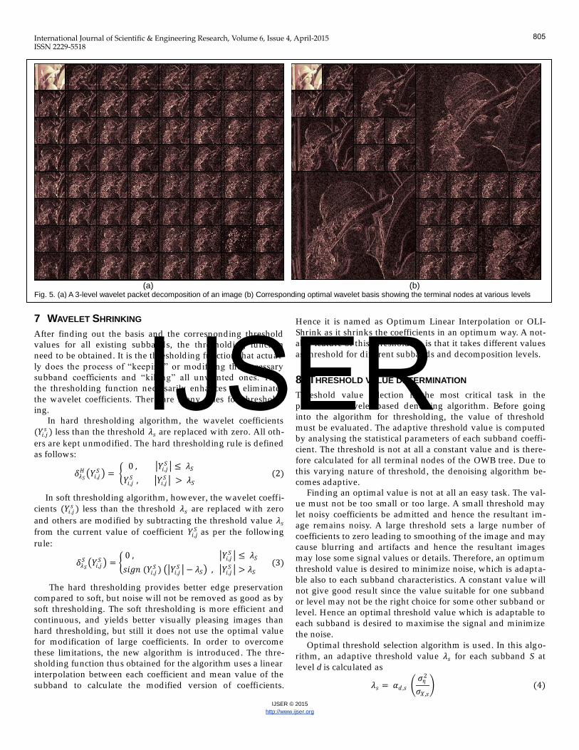
8 THRESHOLD VALUE DETERMINATION

Threshold value selection is the most critical task in the

process of wavelet based denoising algorithm. Before going

into the algorithm for thresholding, the value of threshold

must be evaluated . The adaptive threshold value is computed

by analysing the statistical parameters of each subband coeffi-

cient. The threshold is not at all a constant value and is there-

fore calculated for all terminal nodes of the OWB tree. Due to

this varying nature of threshold , the denoising algorithm be-

comes adaptive.

Finding an optimal value is not at all an easy task. The val-

ue must not be too small or too large. A small threshold may

let noisy coefficients be admitted and hence the resultant im-

age remains noisy. A large threshold sets a large number of

coefficients to zero leading to smoothing of the image and may

cause blurring and artifacts and hence the resultant images

may lose some signal values or details. Therefore, an optimum

threshold value is desired to minimize noise, which is adapt a-

ble also to each subband characteristics. A constant value will

not give good result since the value su itable for one subband

or level may not be the right choice for some other subband or

level. Hence an optimal threshold value which is adaptable to

each subband is desired to maximise the signal and minimize

the noise.

Optimal threshold selection algorithm is used . In this algo-

rithm, an adaptive threshold value 𝜆𝑠 for each subband S at

level d is calculated as

𝜆𝑠 = 𝛼𝑑 ,𝑠 𝜎𝜂

2

𝜎𝑋,𝑠

(4)

(a) (b)

Fig. 5. (a) A 3-level wavelet packet decomposition of an image (b) Corresponding optimal wavelet basis showing the terminal nodes at various levels

805

IJSER


IJSER © 2015


where 𝜎𝜂2 and 𝜎𝑋,𝑠

2 are the variances of noise and clean image

coefficients respectively in the subband S. The noise is as-

sumed to be an additive Gaussian white noise. Since the input

noise variance is unknown, it can be estimated by applying

the median estimator on the HH1 subband’s coefficients (𝑌𝑖 ,𝑗

𝐻𝐻1)

as

𝜎 𝜂 2 =

𝑚𝑒𝑑𝑖𝑎𝑛 |𝑌𝑖,𝑗𝐻𝐻1|

0.6745

2

(5)

Since the noise is additive, the observation model can be

described as 𝑌𝑖 ,𝑗𝑠 = 𝑋𝑖 ,𝑗

𝑠 + 𝜂𝑖 ,𝑗𝑠 where, 𝑌𝑖,𝑗

𝑠 are the noise coeffi-

cients of subband S, 𝑋𝑖 ,𝑗𝑠 are the coefficients of the clean su b-

band (noise free image) and 𝜂𝑖 ,𝑗𝑠 are the noise coefficients. As-

suming that 𝑌𝑖 ,𝑗𝑠 , 𝑋𝑖 ,𝑗

𝑠 , and 𝜂𝑖 ,𝑗𝑠 have generalised Gaussian d is-

tribution models their variances can be written in the form

𝜎𝑌,𝑠2 = 𝜎𝑋,𝑠

2 + 𝜎𝜂2 where 𝜎𝑌,𝑠

2 is the variance of coefficients (𝑌𝑖,𝑗 )

in subband S. From this relation, the signal variance can be

derived as 𝜎𝑋,𝑠2 = 𝑚𝑎𝑥 𝜎𝑌,𝑠

2 − 𝜎𝜂2 , 0 .

In previous methods, the term 𝛼𝑑 ,𝑠 was set to one, but here,

𝛼𝑑 ,𝑠 value is employed to make the threshold su itable in each

decomposition level and the subbands within. In other words,

𝛼𝑑 ,𝑠 is set so as to get a larger threshold for high frequency

subbands based on their level of decomposition.

𝛼𝑑 ,𝑠 term makes the threshold value more dependent on

level d and subband s. Since image information exists more in

the low frequency subband than in the high frequency su b-

band and since the probability of existence of noise in the high

frequency component is greater, applying a greater threshold

value to the high frequency subband reduces the effect of

noise more effectively. Also for two successive levels, as the

level of decomposition is increased , the frequency bandwidths

of the created subbands become more limited . So, the thre-

shold value for L1 should be greater than L2 because the high

frequency components of L1 need to be larger than L2. Thus

𝛼𝑑 ,𝑠 makes the threshold value level and subband dependent.

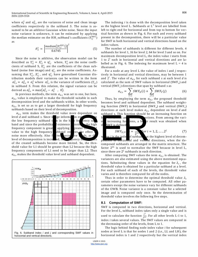
The indexing i is done with the decomposition level taken

as the highest level L. Subbands at Lth level are labelled from

left to right end for horizontal and from top to bottom for ver-

tical function as shown in Fig. 6. For each and every subband

present in the decomposition, there will be a particular value

for SWF in both horizontal and vertical d irections based on the

index values.

The number of subbands is d ifferent for d ifferent levels. 4

subbands for level 1, 16 for level 2, 64 for level 3 and so on. For

maximum decomposition level L, the index value i starts from

1 to 2L each in horizontal and vertical d irections and are la-

belled as in Fig. 6. The indexing for maximum level L = 4 is

illustrated .

For a node at any level L the value of index i and j respec-

tively in horizontal and vertical d irections, may be between 1

and 2L. The value of 𝛼𝑑 ,𝑠 for each subband s at each level d is

calculated as the sum of SWF values in horizontal (SWFH) and

vertical (SWFV) d irections that span by subband s as

𝛼𝑑 ,𝑠 = 𝑆𝑊𝐹𝐻 𝑖

𝑖⊂𝑠

+ 𝑆𝑊𝐹𝑉 𝑗

𝑗⊂𝑠

(6)

Thus, by employing the term 𝛼𝑑 ,𝑠 the proposed threshold

becomes level and subband dependent. The subband weigh t-

ing function (SWF) in horizontal (SWFH) and vertical (SWF

V)

d irections at each level makes 𝛼𝑑 ,𝑠 dependent on level d and

subband s. This function should be an increasing function on

both horizontal and vertical d irections. From among the var i-

ous increasing functions, a better result was obtained when

the SWF is defined as

𝑆𝑊𝐹𝐻 𝑉 𝑖 = 𝑖2

22𝐿 𝑓𝑜𝑟 𝑖 = 1, 2,… . , 2𝐿 (7)

where i is the index of subbands at the highest level of decom-

position in horizontal and vertical d irections, when the d e-

composed subbands are arranged in the matrix structure. The

factor 22𝐿 is used to normalize the SWF because in level L,

since there are 2𝐿 subbands in each d irection.

After computing SWF values the term 𝛼𝑑 ,𝑠 is obtained. The

variances are also estimated using the above mentioned equ a-

tions. Substitu ting these values in the equation for 𝜆𝑠 , the

threshold value is obtained for a particular subband at a level.

For each subband of each of the levels, the threshold value

varies and is therefore computed for all the nodes.

Thus in order to determine the optimal threshold value 𝜆𝑠 certain other parameters have to be computed . All other pa-

rameters except the noise variance vary for d ifferent subbands

of the OWB. Noise variance is a constant value for a selected

image and is computed only once. So the determination of

threshold value involves the following five steps.

8.1 Computation of SWF:

SWF is computed in two directions, horizontal and vertical.

For the level L, subband index takes only a single value and is

used to calculate the function 𝑖2

22𝐿 . For all other levels L-1 to 1,

index i takes several values. The SWF values are computed in

the decreasing order of the levels, from L to 1.

The logic behind finding node index value i for subsequent

nodes at level L is that for nodes 1 and 2 (i.e., LL and LH), the

horizontal index is 1 and 2 respectively but the vert ical index Fig. 6. Subband index i and j and corresponding SWF values in horizontal and vertical directions.

806

IJSER


IJSER © 2015


is 1 for both the nodes. Similarly for nodes 3 and 4 (i.e., HL

and HH), the horizontal indices are 1 and 2, but the vertical

index is 2. Only after assigning index values, the SWF values

can be evaluated .

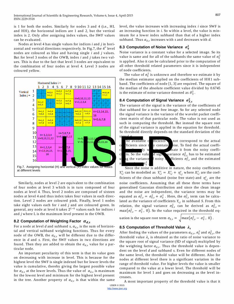
Nodes at level 4 has single values for indices i and j in hori-

zontal and vertical d irections respectively. In Fig.7, the 4th level

nodes are coloured as blue and having single i and j values.

But for level 3 nodes of the OWB, index i and j takes two val-

ues. This is due to the fact that level 3 n odes are equivalent to

the combination of four nodes at level 4. Level 3 nodes are

coloured yellow.

Similarly, nodes at level 2 are equivalent to the combination

of four nodes at level 3 which is in turn composed of four

nodes at level 4. Thus, level 2 nodes are composed of sixteen

nodes at level 4 and thus index takes four values in each d irec-

tion. Level 2 nodes are coloured pink. Finally, level 1 nodes

take eight values each for i and j and are coloured green. In

general, any node at level k takes 2𝐿−𝑘 values each for indices i

and j where L is the maximum level present in the OWB.

8.2 Computation of Weighting Factor 𝜶𝒅,𝒔

For a node at level d and subband s, 𝛼𝑑 ,𝑠 is the sum of horizon-

tal and vertical subband weighting functions. Thus for every

node of the OWB, the 𝛼𝑑 ,𝑠 will be d ifferent due to the d iffer-

ence in d and s. First, the SWF values in two directions are

found . Then they are added to obtain the 𝛼𝑑 ,𝑠 value for a par-

ticular node.

An important peculiarity of this term is that its value goes

on decreasing with increase in level. This is because for the

highest level the SWF is single indexed but for lower levels the

value is cumulative, thereby giving the largest possible value

for 𝛼𝑑 ,𝑠 at the lower levels. Thus the value of 𝛼𝑑 ,𝑠 is maximum

for the lowest level and minimum for the highest level present

in the tree. Another property of 𝛼𝑑 ,𝑠 is that within the same

level, the value increases with increasing index i since SWF is

an increasing function in i. So within a level, the value is min-

imum for a lower index subband than that of a higher index

subband. Thus 𝛼𝑑 ,𝑠 increases with s and decreases with d.

8.3 Computation of Noise Variance 𝝈𝜼𝟐

Noise variance is a constant value for a selected image. So its

value is same and for all of the subbands the same value of 𝜎𝜂2

is applied . Also it can be calculated prior to the computation of

all other threshold related parameters since it is independent

of node coefficients.

The value of 𝜎𝜂2 is unknown and therefore we estimate it by

the median estimator applied on the coefficients of HH1 sub-

band. The coefficients of node [1, 3] are required . The square of

the median of the absolu te coefficient value d ivided by 0.6745

is the estimate of noise variance denoted as 𝜎 𝜂 2 .

8.4 Computation of Signal Variance 𝝈𝑿,𝒔𝟐

The variance of the signal is the variance of the coefficients of

that subband for a noise free image. So for any selected node

the signal variance is the variance of the wavelet packet coeffi-

cient matrix of that particular node. The value is not used as

such in computing the threshold . But instead the square root

of the signal variance is applied in the equation for threshold .

So threshold d irectly depends on the standard deviation of the

signal 𝜎𝑋,𝑠 .

The available coefficients do not correspond to the actual

coefficients since they contain noise. To find the actual coeffi-

cients, the only way is to estimate it from the noisy coeffi-

cients. So the value of signal variance 𝜎𝑋,𝑠2 has to be estimated

using the variance of noisy coefficients 𝜎𝑌,𝑠2 and the estimated

noise variance 𝜎2 .

Since the noise is additive in nature, the noisy coefficients

𝑌𝑖 ,𝑗𝑠 can be modelled as 𝑌𝑖 ,𝑗

𝑠 = 𝑋𝑖 ,𝑗𝑠 +

𝑖 ,𝑗𝑠 where 𝑋𝑖 ,𝑗

𝑠 are the coef-

ficients of the clean subband (noise free state) and 𝑖 ,𝑗𝑠 are the

noise coefficients. Assuming that all these three terms have

generalised Gaussian d istribution and since the clean image

and the noise are independent, the variance terms may be

equated as 𝜎𝑌,𝑠2 = 𝜎𝑋,𝑠

2 + 𝜎2 . Here, the 𝜎𝑌,𝑠

2 term can be calcu-

lated as the variance of coefficients 𝑌𝑖,𝑗 in subband S. From this

relation, the signal variance 𝜎𝑋,𝑠2 can be derived as 𝜎𝑋,𝑠

2 =

𝑚𝑎𝑥 𝜎𝑌,𝑠2 − 𝜎

2 , 0 . So the value required in the threshold eq-

uation is the square root term 𝜎𝑋,𝑠 = 𝑚𝑎𝑥 𝜎𝑌,𝑠2 − 𝜎

2 , 0 .

8.5 Computation of Threshold Value 𝝀𝒔

After finding the values of the parameters 𝛼𝑑 ,𝑠 , 𝜎𝜂2 and 𝜎𝑋,𝑠

2 , the

threshold value 𝜆𝑠 is obtained as the ratio of noise variance to

the square root of signal variance (SD of signal) multiplied by

the weighting factor 𝛼𝑑 ,𝑠 . Thus the threshold value is depen-

dent on the level d and subband s. Even for d ifferent nodes of

the same level, the threshold value will be d ifferent. Also for

nodes at d ifferent level there is a significant variation in the

range of threshold value. For higher levels the value is smaller

compared to the value at a lower level. The threshold will be

maximum for level 1 and goes on decreasing as the level in-

creases.

A most important property of the threshold value is that it

Fig.7. Assigning horizontal (H) and vertical (V) index values for nodes at different levels

807

IJSER


IJSER © 2015


must be relative to the values of the coefficients at d ifferent

levels. The lower level coefficients are larger compared to the

higher levels and therefore the threshold values also need to

be larger at lower levels. Thus the adaptive threshold exactly

follows this requirement due to the decreasing nature of 𝛼𝑑 ,𝑠

with increasing level.

All dynamic terms like 𝛼𝑑 ,𝑠 , and 𝜎𝑋,𝑠2 are computed prior to

the computation of threshold 𝜆𝑠 for each subband s. The thre-

shold meets all required conditions for its adaptive nature due

to the presence of weighting function which is in turn due to

the dependency of SWF on level d and subband s. Since SWF

varies with d and s, the resultant threshold is clearly adaptive

to d and s.

9 THRESHOLDING ALGORITHM

To overcome the shortcomings of the previously used hard

and soft thresholding ru les, a new algorithm is introduced.

The principle behind all thresholding methods is that the coef-

ficients smaller than a specific value or threshold are can-

celled . The new thresholding algorithm called OLI-Shrink uses

optimal linear interpolation between each coefficient and cor-

responding subband mean for the modification of dominant

coefficients. The thresholding function is described as

𝛿𝜆𝑠𝑂𝐿𝐼 𝑌𝑖 ,𝑗

𝑆 = 0, 𝑌𝑖 ,𝑗

𝑆 ≤ 𝜆𝑆

𝑌𝑖 ,𝑗𝑆 − 𝛽 𝑌𝑖 ,𝑗

𝑆 − 𝜇𝑆 , |𝑌𝑖 ,𝑗𝑆 | > 𝜆𝑆

(8)

where 𝜇𝑆 is the mean value of the coefficient of subband s; and

𝛽 is computed as 𝛽 =𝜎𝜂

2

𝜎𝑋 ,𝑠2 +𝜎𝜂

2 ≅

𝜎𝜂2

𝜎𝑌 ,𝑠2 . The thresholding func-

tion is derived using Bayesian MAP estimation of a signal

from its noisy version. Thus the modified coefficient is est i-

mated by a weighted linear interpolation of the unconditional

mean and the observed value of coefficients. Hence this op-

timal linear interpolation between each coefficient and corres-

ponding subband’s mean (MAP based) is combined with

wavelet thresholding algorithm (based on adaptive threshold)

to yield the proposed thresholding function 𝛿𝜆𝑠𝑂𝐿𝐼 . Based on

these analyses, the efficient and simple to implement denois-

ing algorithm may be summarised as follows:

9.1 Proposed Denoising Algorithm

STEP 1 : Perform WP decomposition to obtain OWB.

STEP 2 : Estimate noise variance, 𝜎𝜂2 for the image.

STEP 3 : For each subband S in level d , compute the

statistical parameters:

Subband variance 𝜎𝑌,𝑠2

Subband mean 𝜇𝑠

Clean image variance 𝜎𝑋,𝑠2

Subband weighting factor 𝛼𝑑 ,𝑆

Coefficient weighting factor 𝛽 STEP 4 : Find the threshold value 𝜆𝑆 for all existing

nodes.

STEP 5 : Threshold all subband’s coefficients using the

proposed threshold ing technique ―OLI-

Shrink‖.

STEP 6 : Construct the new tree using modified coeffi-

cients.

STEP 7 : Perform the inverse WPT to reconstruct the

denoised image.

Apart from the threshold value 𝜆𝑆 certain other variable

have to be evaluated before beginning with the thresholding

algorithm. One is the subband mean 𝜇𝑠 which is the mean val-

ue of the coefficients of a selected subband s. This is calculated

separately for every node present in the tree. Another term

required in the thresholding function is the coefficient weigh t-

ing factor 𝛽. It is computed as the ratio between noise variance

and the sum of signal and noise variances. In other words, 𝛽

can be approximated as the ratio of variance of noise 𝜂 to the

variance of the subband coefficients 𝑌𝑖 ,𝑗 .

To apply the thresholding function, each of the coefficient

values 𝑌𝑖 ,𝑗 is to be compared with the previously computed

threshold value 𝜆𝑆 of the corresponding subband s. If the ab-

solu te value of coefficient is smaller than threshold , they are to

be neglected and need not be considered while performing the

inverse transform. Hence such terms are replaced by zero.

Otherwise if the absolu te values of coefficients exceed the

threshold value of that subband, then they are to be modified

to a new value determined by the properties of the subband

which is in turn dependent on the terms 𝜇𝑠 and 𝛽. Thus the

thresholding function is repeatedly applied to all the coeffi-

cients in all the subbands and the new values replace the old

coefficients in the tree. Now a new tree is obtained as a resu lt

of the thresholding function 𝛿𝜆𝑠𝑂𝐿𝐼 . The modified tree with the

new values of coefficients in every subband s then undergoes

an inverse wavelet packet transform to reconstruct the noise-

less or the denoised image.

The thresholding function can be applied alike to both

grayscale and colour images. The only d ifference is that the

coefficient matrix is three d imensional. Hence denoising co-

lour images will take more time than its grayscale counterpart.

10 DENOISING BY MODIFIED OVERCOMPLETE WAVELET

REPRESENTATION

The overcomplete representation is a model based approach

and its performance depends on how well the model fits the

signal and how accurately the parameters are estimated . Here,

a MAP-based approach is followed.

A signal estimation algorithm based on multiple wavelet

representations and Gaussian models is u tilised here. The

proposed method consists of two major steps: optimum est i-

mation of the wavelet coefficients and averaging of the sep a-

rate denoised images. Using over-complete representations

(multiple wavelet transforms) the important image features

can be captured by using the least number of transform coeffi-

cients. Optimum estimation step is carried out by OLI-Shrink

algorithm.

The effective image denoising algorithm is based on the

maximum a posteriori (MAP) estimation principle. Here the

idea of MAP-based estimation is extend ed to the use of two or

more wavelets instead of a single wavelet.

808

IJSER


IJSER © 2015


The proposed method consists of two d istinct WP tran s-

forms followed by a denoising algorithm resulting in two sep-

arate set of wavelet coefficients. The optimal basis and MAP-

based linear thresholding ru les applied to both are the same.

After denoising algorithm, the two WPTs undergo inverse

transform and thereby produce two denoised images. In order

to get a better result the average of the two is taken as final

output. The entire algorithm can be summarised as follows:

10.1 Denoising Algorithm by Modified Overcomplete Wavelet Representation

STEP 1: Perform an L-level wavelet transformation of the noi-

sy image along with OWB extraction procedure using

two wavelets separately, producing two trees of wave-

let coefficients.

STEP 2: Apply the denoising method based on adaptive thre-

sholding function described by OLI-Shrink for the

two trees producing two sets of modified coefficients

(denoised coefficients).

STEP 3: Perform the inverse wavelet transformation resulting

in two denoised images.

STEP 4: Take the average of the denoised images to give the

final denoised image.

The method can be extended to using more than two wave-

lets for denoising. Thus the algorithm performs two or more

individual MAP-based wavelet denoising process and takes

the average of them as the final result.

For denoising, the best result giving OLI-Shrink algorithm

is applied for thresholding. To demonstrate the performance of

this denoising method, the pairs of wavelets with similar

properties are tested . Wavelet pair sym12 and coif4 is chosen

since the wavelet filters are of same length. Other types of

wavelet pair that originate from one orthogonal w avelet are

also taken. One way of forming such a pair is to use an orth o-

gonal wavelet and its double shifted version. Another way of

forming pair is to use an orthogonal wavelet and its reverse

version. Both operations are achieved for orthogonal wavelets

by double shifting or reversing the scaling filter. In actual im-

plementation, double shifting corresponds to the double shift-

ing of all filters while reversing corresponds to using recon-

struction filter for decomposition and decomposition filter for

reconstruction.

The averaging step improves the signal to noise ratio as

long as the noises in each of the denoised images are not corre-

lated . Achieving an acceptable result for OLI-Shrink requires

independent calculation of parameters since each uses d istinct

wavelets for decomposition and threshold computation is

done separately. Thus OC representation is the basic denoising

strategy and its success lies in the efficiency of the denoising

algorithm used in it. Both the approaches improve denoising

and thus their combination leads to better result.

11 PERFORMANCE EVALUATION

The performance of the proposed noise reduction algorithm is

measured with the help of quantitative performance measures

such as peak signal to noise ratio (PSNR) and in terms of the

visual quality of the images using universal image quality in-

dex (UIQI).

11.1 Peak Signal to Noise Ratio (PSNR)

The denoised image will never be same as that of the original

image. So in order to represent the error between two versions

of the same image, the mean squared error (MSE) is u sed . MSE

between the original image X and the denoised image X̂ is

given as

𝑀𝑆𝐸 = 1

𝑀𝑁 (𝑋 𝑖, 𝑗 − X̂ 𝑖, 𝑗 )2

𝑁

𝑗=1

𝑀

𝑖=1

(9)

where M and N are the width and height of the image respec-

tively. Now the PSNR is calculated on the basis of MSE. For

the denoised image the PSNR is given by

𝑃𝑆𝑁𝑅 𝑋, X̂ = 10 log10 2552

𝑀𝑆𝐸 𝑑𝐵 (10)

11.2 Universal Image Quality Index (UIQI)

The performance of most of the algorithms is evaluated by

computing the Peak Signal to Noise Ratio (PSNR) alone. The

PSNR is purely a mathematical measure and does not contain

any indication about the perceived quality. It was in 2002 that,

Zhou Wang and Alan C. Bovik introduced a new objective

image quality index called the Universal Image Quality Index

(UIQI) [18] which signifies perceptual quality. UIQI is a new

objective image quality index which signifies the perceptual

quality of images and is calculated based on their visual quali-

ty. The index is universal in the sense it does not depend on

the images being tested , viewing conditions or individual ob-

servers. The universal image quality index is given by:

𝑈𝐼𝑄𝐼 𝑋,𝑋 = 4𝜎 𝑋 ,𝑋 ̂ 𝜇𝑋 𝜇𝑋 ̂

𝜎𝑋2 + 𝜎X̂

2 𝜇𝑋2 + 𝜇X̂

2 (11)

where 𝜎 𝑋,�̂� is the covariance of X and X̂, 𝜇𝑋 , 𝜇�̂� are the mean

values of X and X̂ and 𝜎𝑋2, 𝜎X̂

2 are the variances of X and X̂.

UIQI is a real number between 0 and 1 inclusive. The best va l-

ue UIQI = 1 is achieved if and only if X = X̂. UIQI is designed

by modeling image d istortion as a combination of three d istor-

tions related to correlation, luminance and contrast. UIQI

models the total d istortion in an image as a combination of the

three factors:

1) Loss of correlation

2) Luminance d istortion

3) Contrast d istortion

UIQI represents each of them as 𝑈𝐼𝑄𝐼 = 𝜎 𝑋 ,𝑋

𝜎𝑋𝜎𝑋 .

2𝜇𝑋𝜇𝑋

𝜇𝑋2 +𝜇

𝑋 2 .

2𝜎𝑋𝜎𝑋

𝜎𝑋2 +𝜎

𝑋 2 .

Here, the first term refers to the correlation coefficient that

measures the degree of linear correlation between X and X̂ and

lies in the range [-1, 1]. The second term is the luminance d is-

tribution that measures how close is the mean luminance be-

tween X and X̂. This value is in the range [0, 1] and is equal to

1 only if X=

X̂ . The last term is the contrast d istribution wh ich

measures how similar the contrasts of the images X and X̂ are.

This also lies in the range [0, 1] and becomes 1 if and only if

σX= σ

X̂ since σ

X and σ

X̂ give an estimate of the contrasts of X and

809

IJSER


IJSER © 2015


X̂ respectively. In short, images of better visual appearance

have higher Q value. Thus it outperforms the MSE significan t-

ly in characterizing images under d ifferent types of image d is-

tortions.

12 RESULT AND DISCUSSION

The denoising is implemented and all the related decomposi-

tion, processing and reconstruction are done using MATLAB

version 7.5.0. with the help of wavelet toolbox and associated

functions. The entire algorithm can be applied to grayscale as

well as colour images identically.

The test images are contaminated by Gaussian white noise

at eight d ifferent standard deviations σ = 5, 10, 15, 20, 30, 40,

50, 60. Noise addition is done by adding a random matrix

multiplied by the noise variance to the image matrix. The

MATLAB code for the entire procedure consists of around 800

lines. The code was run using Intel Core i5 processor with in-

ternal RAM capacity of 4 GB sup ported by a 64-bit Windows

Home Basic operating system. The average computational

time is 8 to 15 seconds for noise intensities of σ = 5 to σ = 60

and maximum decomposition level L= 4.

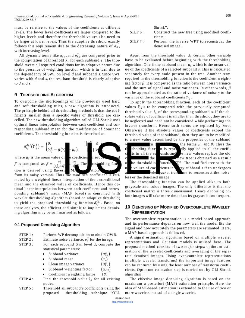
The OWB is a subtree that contains selected nodes and the

decomposition is critical in applying the rest of the algorithm

steps. The OWB obtained for several images is given in Fig. 8.

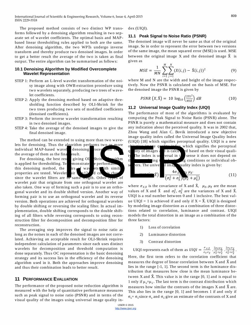
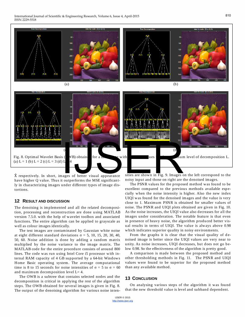
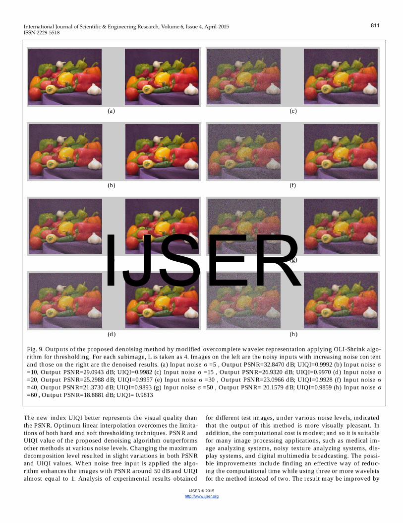
The output of the denoising algorithm for various noise in ten-

s

sities are shown in Fig. 9. Images on the left correspond to the

noisy input and those on right are the denoised images.

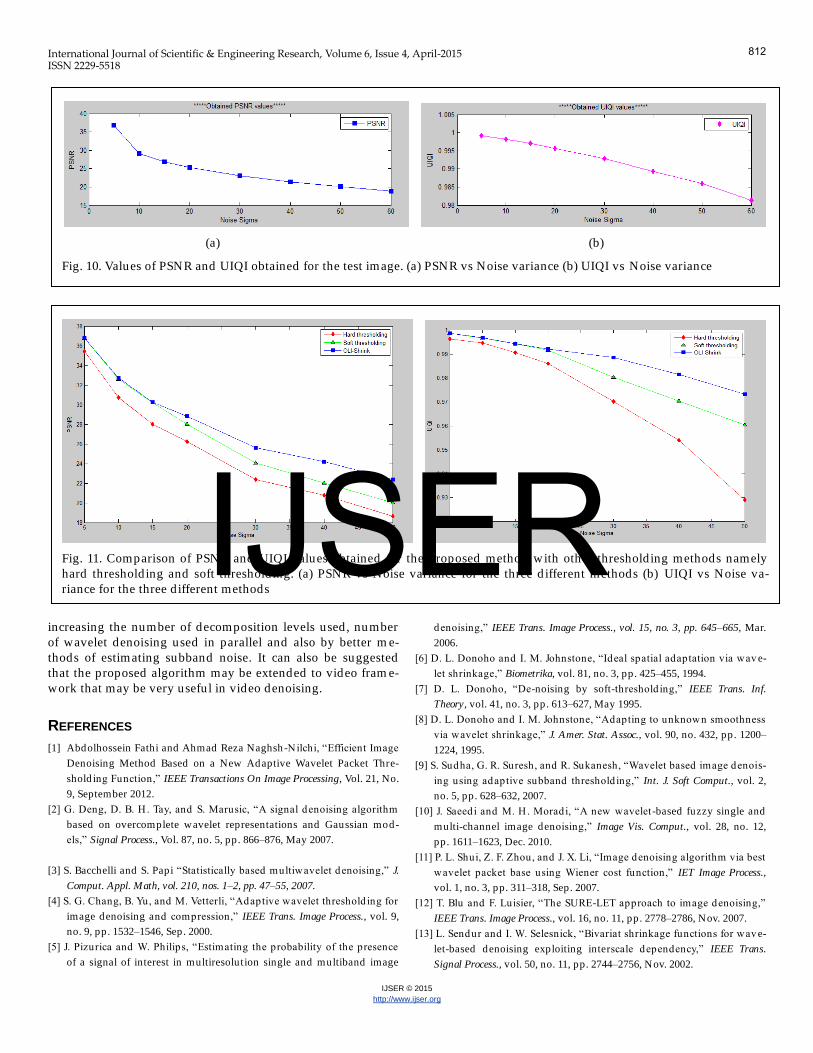
The PSNR values for the proposed method was found to be

excellent compared to the previous methods available esp e-

cially when the noise intensity is higher. Also the new index

UIQI was found for the denoised images and the value is very

close to 1. Maximum PSNR is obtained for smaller values of

noise. The PSNR and UIQI p lots obtained are given in Fig. 10.

As the noise increases, the UIQI value also decreases for a ll the

images under consideration. The notable feature is that even

in presence of heavy noise, the algorithm produced better vis-

ual results in terms of UIQI. The value is always above 0.98

which indicates superior quality in noisy environments.

From the graphs it is clear that the visual quality of d e-

noised image is better since the UIQI values are very near to

unity. As noise increases, UIQI decreases, but does not go be-

low 0.98. So the effectiveness of the algorithm is pretty good.

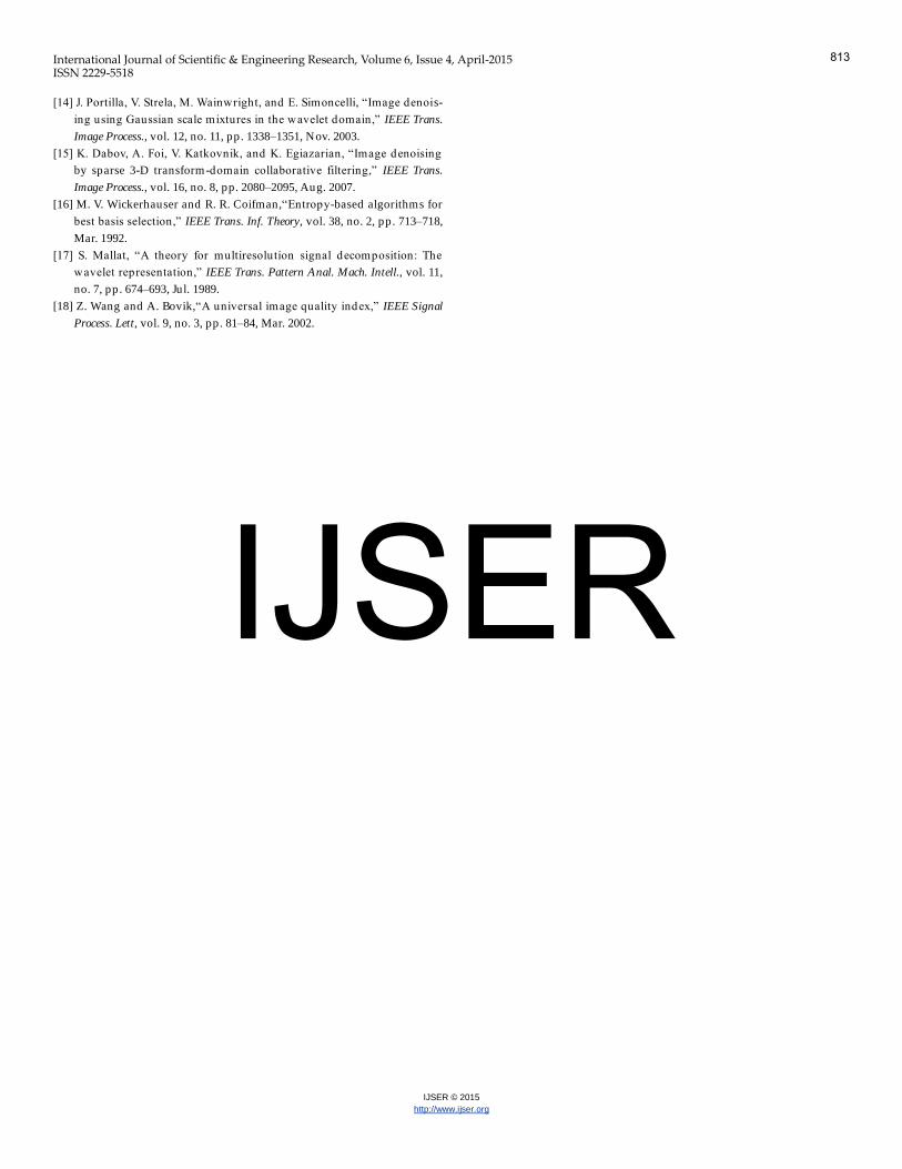
A comparison is made between the proposed method and

other thresholding methods in Fig. 11. The PSNR and UIQI

values were found to be superior for the proposed method

than any available method.

13 CONCLUSION

On analysing various steps of the algorithm it was found

that the new threshold value is level and subband dependent.

(a) (b)

(c) (d)

Fig. 8. Optimal Wavelet Basis (OWB) obtained for a test image with d ifferent values for the maximum level of decomposition L.

(a) L = 1 (b) L = 2 (c) L = 3 (d) L = 4

810

IJSER


IJSER © 2015


The new index UIQI better represents the visual quality than

the PSNR. Optimum linear interpolation overcomes the limita-

tions of both hard and soft thresholding techniques. PSNR and

UIQI value of the proposed denoising algorithm outperforms

other methods at various noise levels. Changing the maximum

decomposition level resulted in slight variations in both PSNR

and UIQI values. When noise free input is applied the algo-

rithm enhances the images with PSNR around 50 dB and UIQI

almost equal to 1. Analysis of experimental results obtained

for d ifferent test images, under various noise levels, ind icated

that the output of this method is more visually pleasant. In

addition, the computational cost is modest; and so it is su itable

for many image processing applications, such as medical im-

age analyzing systems, noisy texture analyzing systems, d is-

play systems, and d igital multimedia broadcasting. The possi-

ble improvements include finding an effective way of redu c-

ing the computational time while using three or more wavelets

for the method instead of two. The result may be improved by

(a) (e)

(b) (f)

(c) (g)

(d) (h)

Fig. 9. Outputs of the proposed denoising method by modified overcomplete wavelet representation applying OLI-Shrink algo-

rithm for thresholding. For each subimage, L is taken as 4. Images on the left are the noisy inputs with increasing noise con tent

and those on the right are the denoised results. (a) Input noise σ =5 , Output PSNR=32.8470 dB; UIQI=0.9992 (b) Input noise σ

=10, Output PSNR=29.0943 dB; UIQI=0.9982 (c) Input noise σ =15 , Output PSNR=26.9320 dB; UIQI=0.9970 (d) Input noise σ

=20, Output PSNR=25.2988 dB; UIQI=0.9957 (e) Input noise σ =30 , Output PSNR=23.0966 dB; UIQI=0.9928 (f) Input noise σ

=40, Output PSNR=21.3730 dB; UIQI=0.9893 (g) Input noise σ =50 , Output PSNR= 20.1579 dB; UIQI=0.9859 (h) Input noise σ

=60 , Output PSNR=18.8881 dB; UIQI= 0.9813

811

IJSER


IJSER © 2015


increasing the number of decomposition levels used , number

of wavelet denoising used in parallel and also by better m e-

thods of estimating subband noise. It can also be suggested

that the proposed algorithm may be extended to video fram e-

work that may be very useful in video denoising.

REFERENCES

[1] Abdolhossein Fathi and Ahmad Reza Naghsh -Nilchi, ―Efficient Image

Denoising Method Based on a New Adaptive Wavelet Packet Thre-

shold ing Function,‖ IEEE Transactions On Image Processing, Vol. 21, No.

9, September 2012.

[2] G. Deng, D. B. H. Tay, and S. Marusic, ―A signal denoising algorithm

based on overcomplete wavelet representations and Gaussian mod-

els,‖ Signal Process., Vol. 87, no. 5, pp. 866–876, May 2007.

[3] S. Bacchelli and S. Papi ―Statistically based multiwavelet denoising,‖ J.

Comput. Appl. Math, vol. 210, nos. 1–2, pp. 47–55, 2007.

[4] S. G. Chang, B. Yu, and M. Vetterli, ―Adaptive wavelet threshold ing for

image denoising and compression,‖ IEEE Trans. Image Process., vol. 9,

no. 9, pp. 1532–1546, Sep. 2000.

[5] J. Pizurica and W. Philips, ―Estimating the probability of the presence

of a signal of interest in multiresolution single and multiband image

denoising,‖ IEEE Trans. Image Process., vol. 15, no. 3, pp. 645–665, Mar.

2006.

[6] D. L. Donoho and I. M. Johnstone, ―Ideal spatial adaptation via wav e-

let shrinkage,‖ Biometrika, vol. 81, no. 3, pp. 425–455, 1994.

[7] D. L. Donoho, ―De-noising by soft-threshold ing,‖ IEEE Trans. Inf.

Theory, vol. 41, no. 3, pp. 613–627, May 1995.

[8] D. L. Donoho and I. M. Johnstone, ―Adapting to unknown smoothness

via wavelet shrinkage,‖ J. Amer. Stat. Assoc., vol. 90, no. 432, pp. 1200–

1224, 1995.

[9] S. Sudha, G. R. Suresh, and R. Sukanesh, ―Wavelet based image denois-

ing using adaptive subband threshold ing,‖ Int. J. Soft Comput., vol. 2,

no. 5, pp. 628–632, 2007.

[10] J. Saeedi and M. H. Moradi, ―A new wavelet-based fuzzy single and

multi-channel image denoising,‖ Image Vis. Comput., vol. 28, no. 12,

pp. 1611–1623, Dec. 2010.

[11] P. L. Shui, Z. F. Zhou, and J. X. Li, ―Image denoising algorithm via best

wavelet packet base using Wiener cost function,‖ IET Image Process.,

vol. 1, no. 3, pp. 311–318, Sep. 2007.

[12] T. Blu and F. Luisier, ―The SURE-LET approach to image denoising,‖

IEEE Trans. Image Process., vol. 16, no. 11, pp. 2778–2786, Nov. 2007.

[13] L. Sendur and I. W. Selesnick, ―Bivariat shrinkage functions for wav e-

let-based denoising exploiting interscale dependency,‖ IEEE Trans.

Signal Process., vol. 50, no. 11, pp. 2744–2756, Nov. 2002.

(a) (b)

Fig. 10. Values of PSNR and UIQI obtained for the test image. (a) PSNR vs Noise variance (b) UIQI vs Noise variance

Fig. 11. Comparison of PSNR and UIQI values obtained for the proposed method w ith other thresholding methods namely

hard thresholding and soft thresholding. (a) PSNR vs Noise variance for the three d ifferent methods (b) UIQI vs Noise va-

riance for the three d ifferent methods

812

IJSER


IJSER © 2015


[14] J. Portilla, V. Strela, M. Wainwright, and E. Simoncelli, ―Image denois-

ing using Gaussian scale mixtures in the wavelet domain,‖ IEEE Trans.

Image Process., vol. 12, no. 11, pp. 1338–1351, Nov. 2003.

[15] K. Dabov, A. Foi, V. Katkovnik, and K. Egiazarian, ―Image denoising

by sparse 3-D transform-domain collaborative filtering,‖ IEEE Trans.

Image Process., vol. 16, no. 8, pp. 2080–2095, Aug. 2007.

[16] M. V. Wickerhauser and R. R. Coifman,―Entropy-based algorithms for

best basis selection,‖ IEEE Trans. Inf. Theory, vol. 38, no. 2, pp. 713–718,

Mar. 1992.

[17] S. Mallat, ―A theory for multiresolution signal decomposition: The

wavelet representation,‖ IEEE Trans. Pattern Anal. Mach. Intell., vol. 11,

no. 7, pp. 674–693, Jul. 1989.

[18] Z. Wang and A. Bovik,―A universal image quality index,‖ IEEE Signal

Process. Lett, vol. 9, no. 3, pp. 81–84, Mar. 2002.

813

IJSER

Documents

Image Denoising by Modified Overcomplete Wavelet ... · Image Denoising by Modified Overcomplete Wavelet Representation Utilizing Adaptive Thresholding Algorithm Jitha C R Abstract—