Embed Size (px)
Citation preview
Corso di Laurea Triennale in Fisica
Landau diamagnetismand
de Haas-van Alphen oscillations
Relatore:prof. Luca Guido Molinari
Tesi di Laurea di:Lorenzo De Ros
Matricola: 907979
Anno Accademico 2019/2020
Contents
1 Introduction 31.1 Summary . . . . . . . . . . . . . . . . . . . . . . . . . . . . . . . . 31.2 History of the observations . . . . . . . . . . . . . . . . . . . . . . . 61.3 The external magnetic field H . . . . . . . . . . . . . . . . . . . . . 7
2 Statistical mechanics 82.1 Classical statistical mechanics . . . . . . . . . . . . . . . . . . . . . 82.2 Quantum statistical mechanics . . . . . . . . . . . . . . . . . . . . . 9
3 Classical treatment 11
4 Onsager semiclassical treatment 134.1 Semiclassical motion . . . . . . . . . . . . . . . . . . . . . . . . . . 134.2 Bohr-Sommerfeld quantization . . . . . . . . . . . . . . . . . . . . . 144.3 Onsager derivation of the de Haas-van Alphen oscillations frequency 154.4 Tomography of the Fermi surface . . . . . . . . . . . . . . . . . . . 17
5 Quantum treatment 185.1 Landau levels . . . . . . . . . . . . . . . . . . . . . . . . . . . . . . 185.2 Degeneracy of Landau levels . . . . . . . . . . . . . . . . . . . . . . 20
6 Landau’s approach 226.1 Landau’s derivation of diamagnetism . . . . . . . . . . . . . . . . . 226.2 Simplified model of de Haas-van Alphen oscillations . . . . . . . . . 24
7 Peierls’ method 267.1 Mathematics behind the method . . . . . . . . . . . . . . . . . . . . 267.2 2D derivation . . . . . . . . . . . . . . . . . . . . . . . . . . . . . . 28
7.2.1 Boltzmann partition function . . . . . . . . . . . . . . . . . 287.2.2 The integral in 2D . . . . . . . . . . . . . . . . . . . . . . . 287.2.3 Pauli paramagnetism and Landau diamagnetism . . . . . . . 297.2.4 The de Haas-van Alphen effect . . . . . . . . . . . . . . . . 30
7.3 3D derivation . . . . . . . . . . . . . . . . . . . . . . . . . . . . . . 327.3.1 Boltzmann partition function . . . . . . . . . . . . . . . . . 327.3.2 The integral in 3D . . . . . . . . . . . . . . . . . . . . . . . 337.3.3 Pauli paramagnetism and Landau diamagnetism . . . . . . . 347.3.4 The de Haas-van Alphen effect . . . . . . . . . . . . . . . . 35
7.4 Comparing semiclassical and quantum results . . . . . . . . . . . . 36
1
CONTENTS 2
A 37A.1 Proof of the resultant formula . . . . . . . . . . . . . . . . . . . . . 37A.2 Hankel representation of Euler Γ function . . . . . . . . . . . . . . . 37A.3 The integral of cos(αt)
cosh2(t). . . . . . . . . . . . . . . . . . . . . . . . . . 38
B The free electron gas 39B.1 2D calculations . . . . . . . . . . . . . . . . . . . . . . . . . . . . . 39B.2 3D calculations . . . . . . . . . . . . . . . . . . . . . . . . . . . . . 39
Chapter 1
Introduction
1.1 SummaryAn electron can interact with a uniform magnetic field in 2 ways: through spin-fieldcoupling and through orbit-field coupling. The first interaction is at the base ofPauli paramagnetism, discovered by Wolfgang Pauli in 1927, and the second inter-action underlies Landau diamagnetism and de Haas-van Alphen effect, predictedand observed in 1930.
In this work we will concentrate on the consequences of this second coupling.In particular we will first analyse the case of a Bloch electron (electron in a lat-tice subject to a periodic potential) in a semiclassical context and we will obtainthe quantization of the orbits’ radius and energy. Moreover, we will deduce aperiodicity in the structure of orbits to vary the field strength.
Then we will take into consideration the case of an almost free electron gas,which is a good approximation of the weakly bound electrons inside a metal. Inthis context it is possible to calculate analitically the magnetization, which happensto be composed of 2 factors: the first one linear in the field and the second oneoscillating.
The frequencies of the oscillations for the Bloch electron and for the almost freeelectron gas are coherent and they are directly related to the geometry of the Fermisurface. The shape of the Fermi surface is involved in a lot of different phenomena(such as transport coefficients and optical characteristics) and the cited relationturns out to be a tool to measure it.
In particular, we now outline the major points of this work. First of all, we con-textualise the canonical and grand canonical partition functions and free energiesin the classical and quantum case for an electron gas assumed to be non interacting.In this treatment the classical Boltzmann single particle partition function
Z1 =
∫Ω1
d3xd3p
h3e−βϵ(x,p)
the quantum Boltzmann single particle partition function
Z1 =∑α
gαe−βϵα
3
CHAPTER 1. INTRODUCTION 4
and the quantum grand canonical potential
Ω = − 1
β
∑α
gα ln(1 + e−β(ϵα−µ)
)have been used. The quantum grand canonical potential is directly connected withthe average magnetization thanks to the relation ⟨M⟩ = − 1
V∂Ω∂H
N
, hence to themagnetic susceptibility, which is defined as χ = ∂⟨M⟩
∂H.
We start by analysing the response of a free electron gas in a classical framework,which leads to the absence of diamagnetism. This result is known as Bohr-vanLeeuwen theorem and it proves that paramagnetism and diamagnetism must havea quantum origin.
Then we study the behaviour of a Bloch electron in a semiclassical frameworkand, using Bohr-Sommerfeld quantization of the action, we obtain an estimateof the fundamental frequency of de Haas-van Alphen oscillations in the magneticsusceptibility and its relation with the geometry of the Fermi surface
∆
(1
H
)=
2πe
ℏcSex(ϵF )
where Sex(ϵF ) is the extremal cross section in k space of the Fermi surface evaluatedat the Fermi energy.
At this point, we give an exact quantum treatment of an electron in a uniformmagnetic field (Landau quantization and degeneracy of Landau levels) startingfrom the Hamiltonian
h =1
2m∗
(p+ e
A(r)
c
)2
− µ · H
and obtaining the eigenvalue spectrum
ϵkzmsn = ℏωc
(n+
1
2
)+
ℏ2k2z2m∗ +msµBH
with degeneracy at fixed kz equal to g = AeH2πℏc and the eigenfunctions
ψkxkzmsn(y) =1√
2nn!lπ1/4e−
(y−y0)2
2l2 Hn
(y − y0l
)ei(kxx+kzz)
Afterwards, we follow Landau’s original derivation of the diamagnetic suscepti-bility of an electron gas in the case of low fields. He calculated the grand canonicalpotential by approximating the series
Ωdia = − eHV
β2π2ℏc
∞∑n=0
∫ +∞
−∞dkz ln
(1 + e
−β
(ℏ2k2z2m∗ +ℏωc(n+ 1
2)−µ
))with an integral thanks to Euler-Maclaurin formula. This leads to
χdia = −1
3
( mm∗
)2 µ2B
Vρ(ϵF ) = −1
3
( mm∗
)2χpara
CHAPTER 1. INTRODUCTION 5
which highlights the relation between the magnetic susceptibility due to the spin-field coupling (Pauli paramagnetism) and the one due to the orbit-field coupling(Landau diamagnetism).
In the end we obtain the magnetization and the magnetic susceptibility of a 2Dand 3D electron gas by using Peierls’ method. This exploits the relation betweenthe grand canonical potential and the Boltzmann single particle partition function
Ω =
∫ +∞
0
dϵdf(ϵ)
dϵL −1
[Z(s)
s2
](ϵ)
The calculation of the inverse Laplace transform requires an integral in the com-plex plane, done thanks to the residue theorem. It results that the grand canonicalpotential, hence also its derivatives (the magnetization and the magnetic suscep-tibility), is composed of 3 addends: Pauli paramagnetism, Landau diamagnetismand de Haas-van Alphen oscillations.
The first two addends are identical to the ones found by Landau, as long as wesubstitute the 2D or 3D density of states at the Fermi energy. The last addend, inthe case of a 2D gas, is
Ωosc =AeH
πℏcβ
+∞∑n=1
(−)n
ncos
(nπ
m∗
m
) cos(
2nπµℏωc
)sinh
(2nπ2
βℏωc
)and in the case of a 3D gas becomes
Ω =V
2π2β
(eH
ℏc
)3/2 +∞∑n=1
(−)n
n3/2cos
(nπ
m∗
m
) cos(
2nπµℏωc
− π4
)sinh
(2π2nβℏωc
)This result is coherent with the semiclassical one obtained by Onsager, but lessgeneral, since it requires the electron gas to be almost free, which means that theFermi surface is required to be almost spherical.
CHAPTER 1. INTRODUCTION 6
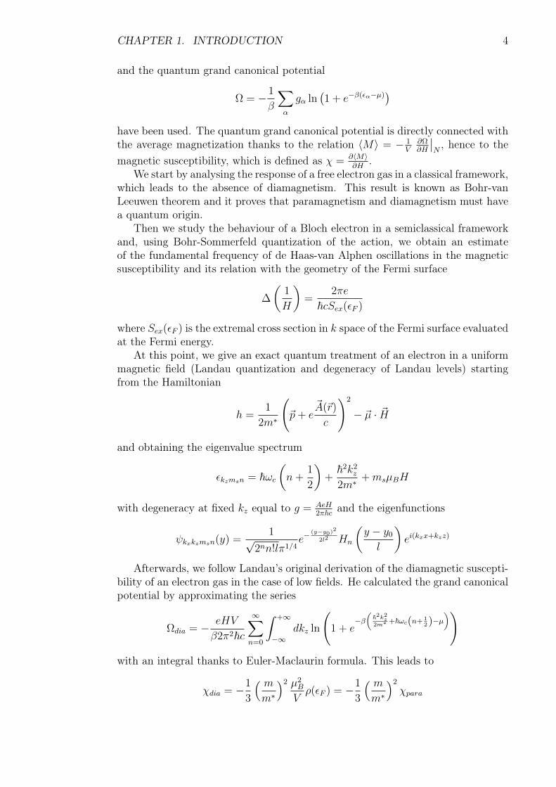
Figure 1.1: First observation of de Haas-van Alphen effect made by de Haas andvan Alphen. We can see the experimental values of the magnetic susceptibilityχ as a function of the external field H. The dependence of the susceptibility ofdiamagnetic metals upon the field, W. J. De Haas and P. M. Van Alphen, 1930.
1.2 History of the observationsW. J. de Haas was a physicist and a professor at Leiden university, Netherlands.In the late 1920s, he discovered, together with L. V. Shubnikov, the Shubnikov-deHaas effect, which is an oscillation in the conductivity of a material that occursat low temperatures as a function of very intense magnetic fields. This was theinspiration that led De Haas and his student P. M. van Alphen in 1930 to measurethe magnetization M of a sample of bismuth as a function of magnetic field inconditions of high fields at 14.2 K and to find oscillations in M/H (figure 1). Themain technique exploited to measure the oscillations is based on the fact thatin a field a magnetized sample experiences a torque proportional to its magneticmoment. This leads to the measure of the oscillations in angular postion of asample of the metal, attached to a filar suspension, as the magnetic field strengthvaries.
Earlier that year, the 22-year-old Lev Landau, a Soviet physicist, was able toaccount for the oscillations in free electron theory, as a direct consequence of thequantization of closed electronic orbits in a magnetic field, and thus as a directobservational manifestation of a purely quantum phenomenon. He also pointedout a -1/3 ratio between the diamagnetic susceptibility he found and the alreadyknown paramagnetic susceptibility discovered by Pauli in 1927.
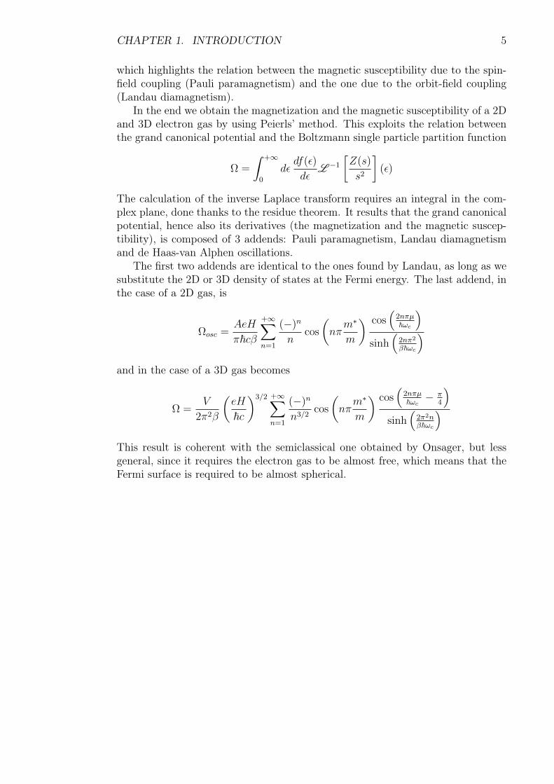
The theory for anisotropic system was put forward by Blackman in 1937 andcompared with the experimental datas for the bismuth susceptibility (figure 2). In1951, Sondheimer and Wilson were the first to evaluate the grand canonical po-tential for the electron gas immersed in a uniform magnetic field exploting Peierls’method, as it is done in this work.
The full extent of the usefulness of measuring the oscillations of the diamagneticsuscpetibility of the metals was only pointed out in 1952 by Onsager. He relatedthe frequency of the oscillations to the shape of the Fermi surface, building a toolfor its measurement. In 1952, Dingle explained that if collision broadening of theenergy levels is taken into account, an extra damping factor must be included inequation (Dingle factor).
CHAPTER 1. INTRODUCTION 7
Figure 1.2: Blackman’s comparison of the experimental χ − H curves with thetheoretical curves for T = 0, (a) when the field is along the binary axis, (b) whenthe field is perpendicular to the binary axis. The experimental points are indicatedin the curves. The susceptibility per unit volume is obtained by multiplying theordinate by 9 · 8 × 10−6, the susceptibility per unit mass by multiplying by 10−6.The unit for the abscissa is 103G. On the diamagnetic susceptibility of bismuth, M.Blackman, 1938.
1.3 The external magnetic field H
In this work we calculate the average magnetization per unit volume, which willbe derived thanks to the relation ⟨M⟩ = − 1
V∂F∂H
N
. F represents the canonicalfree energy (it can be replaced with the grand canonical free energy Ω), which willbe defined in the next chapter. The magnetic susceptibility is defined as χ := ∂M
∂H,
where H is the external magnetic field, which is related to B through the equationB = H + 4πM .
Since in an experiment we have control on H and 4πM is a negligible correctionin comparison with H, we calculate M taking the derivative with respect to H andsubstituting H in place of B everywhere in the following derivations.
Chapter 2
Statistical mechanics
2.1 Classical statistical mechanicsFrom a classical point of view, our system is a gas composed of point particles withelectric charge −e. We define the canonical partition function of the system
Z :=
∫Ω
d3Nxd3Np
N !h3Ne−βE (2.1)
where E is the total energy of the gas and the N ! factor is due to the fact thatinterchanging the coordinates of two electrons gives rise to a classically equivalentconfiguration of the system. The integral is taken over the phase space volume Ωof allowed configurations of the system and the presence of the Planck constant isjust an arbitrary normalization.
The considered system is an ideal gas in the sense that we assumed the electronsto be non interacting, and thanks to this hypothesis we can write the total energy ofthe gas as E =
∑Ni=1 ϵ(xi, pi), where ϵ(xi, pi) is the single particle energy, function
of the 6 coordinates xi and pi in the phase space.
Therefore the partition function can be factored as Z = 1N !
N∏i=1
Zi = 1N !ZN
1 ,
whereZ1 =
∫Ω1
d3xd3p
h3e−βϵ(x,p) (2.2)
since the energy of each electron ϵ is the same function of the coordinates xi and pi.The canonical partition function Z contains all the information about the systemand it can be used to calculate the canonical free energy
F := − 1
βln(Z) (2.3)
which for a non interacting gas becomes
F = −Nβ
ln
(Z1
N !
)(2.4)
The average magnetization, which we are interested in, is defined in the canonicalensemble as < M >= − ∂F
∂H.
8
CHAPTER 2. STATISTICAL MECHANICS 9
2.2 Quantum statistical mechanicsElectrons are fermions with s = 1/2. In our system we have a certain number ofelectrons confined inside a box. The global wave function of all electrons, sincethey have semi-integer spin, must be antisymmetric under interchange of any 2electrons. Pauli exclusion principle is a direct consequence of this global wavefunction characteristic and it states that 2 identical fermions (in our case electrons)can never occupy the same quantum state, otherwise the global wave functionwould be symmetric under their interchange. This fact plays a very important rolein the behaviour of an electron gas, expecially at low temperature, which is ourcase.
In our analysis the electrons are assumed to be non interacting, therefore theglobal Hamiltonian H can be decomposed as the sum of the N single electronHamiltonians h
H =N∑j=1
h(pj, rj, σj) (2.5)
where pj, rj and σj are respectively the momentum, position and spin operatorsof the j-th electron. The operators relative to different electrons commute, hencethe single particle Hamiltonians [h(pi, ri, σi), h(pj, rj, σj)] = 0 So, in general, thesingle electron wave function is a solution of the equation hψk = ϵkψk, with ϵkeigenvalue of the k-th eigenstate of the single electron Hamiltonian. Now the wavefunction of a generic state of the system is built antisymmetrising the consideredsingle particle eigenfunctions (Slater determinant) as follows
Ψ(r1, σ1, ..., rN , σN) =1√N !
∑P
(−)P∏k
ψk(rP (1), σP (1), ..., rP (N), σP (N)) (2.6)
where the sum is taken over all possible permutations P of the electron index andthe product is taken over the k single particle eigenstates considered.
Ψk is the k-th solution of the Schrödinger equation HΨk = EkΨk and using therelations (2.5) and (2.6), we obtain E =
∑k ϵk which means that the energy of the
state of a set of non interacting electrons is the sum of the energies of the statesthat have been antisymmetrised to build it.
Now we analyse in a quantum context the already mentioned single particlecanonical partition function particle (2.2)
Z1 := tr(e−βh
)=∑k
e−βϵk =∑α
gαe−βϵα (2.7)
where the trace is taken over all possible eigenfunction ψk of the operator h. Thisis equivalent to summing over all possible ϵα eingenvalues of h taking into accountthe degeneracy of each eigenvalue gα.
We also introduce the grand canonical partition function Ξ of the system, whichis defined as
Ξ := tr(e−β(H−µN)
)(2.8)
CHAPTER 2. STATISTICAL MECHANICS 10
where N intended as an operator and µ is called the chemical potential. Now weelaborate the formula in our conditions
Ξ =∞∑
N=0
∑k
e−β(∑
k ϵk−µN) =
where the first sum is taken over all possible N numbers of electrons and the secondsum is taken over all possible k eigenstates of the system’s Hamiltonian H. Thisis equivalent to the summation
=∞∑
N=0
∑nk
e−β∑
k(ϵk−µ)nk =∞∑
N=0
∑nk
∏k
e−β(ϵk−µ)nk =
where nk is the number of electrons occupying the k-th eigenstate with the restric-tion
∑k nk = N . Extending the second summation over all possible nk, we can
remove the last condition and the summation over all possible N . Therefore
=∑nk
∏k
e−β(ϵk−µ)nk =∏k
∑n
e−β(ϵk−µ)n =∏k
(1 + e−β(ϵk−µ)
)since two fermions can never occupy the same quantum state, so the only possibil-ities are n = 0, 1
Ξ =∏k
(1 + e−β(ϵk−µ)
)(2.9)
The last quantity we introduce is the grand canonical potential (grand canonicalfree energy), which is defined as
Ω := − 1
βln Ξ (2.10)
and thanks to equation (2.9) we can write in our context
Ω = − 1
β
∑k
ln(1 + e−β(ϵk−µ)
)= − 1
β
∑α
gα ln(1 + e−β(ϵα−µ)
)(2.11)
From the grand canonical potential, the average magnetization, which we areinterested in, is defined in the grand canonical ensemble as < M >:= − 1
V∂Ω∂H
andsimilarly the average number of electrons < N >:= −∂Ω
∂µ.
Chapter 3
Classical treatment
Bohr-van Leeuwen theorem states that diamagnetism can not occur in a classicalsystem at the equilibrium. First we give a non-formal insight on the 2D phe-nomenon.
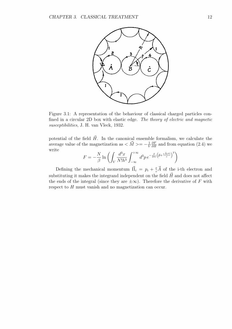
We consider N electrons confined inside a 2D large circular box of radius R asin figure 3.1. The collisions of the electrons with the edge of the box are assumedto be elastic. The area of the box is A = πR2 and the density of the electronsn = N
Ais uniform inside the box. The electrons are immersed in a magnetic field
orthogonal to the 2D box, therefore each electron is subject to the Lorentz forceF = − e
cv×H, which is a centripetal force since it is by definition orthogonal to the
velocity. We obtain the relation for the magnitude mv2
r= e
cvH. This causes the
trajectories to be circumferences of radius r = vωc
, where ωc :=eHmc
is the cyclotronfrequency, all run in the same direction.
The magnetic moment of each electron can be calculated as µ = − eL2m
whereL = ρ × mv is the angular momentum of the considered electron with respectto an origin common to every electron. We choose the common origin to be, forinstance, the point B in figure 3.1. When electron 2 passes through the smallelement enclosed by the square, it has the same angular momentum of electron 1when it passes through this element, but with opposite direction. Since electronsare uniformly distributed in the box, it is clear that for each electron passingthrough a given point in the box with a certain velocity, there is another electronpassing through the same point with the same velocity but with opposite direction.The electrons near the boundary, like electron 1, collide with the edge and bounceelastically along the edge, forming a sequence of arcs of circumference. Theseelectrons play a fundamental role in the absence of diamagnetism in classical modelsbecause, without them, electrons passing near the edge can not be compensated.
Now we exhibit a formal proof. We consider N electrons as a 3D classical ideal(non interacting) gas of charged particles in a volume V . The magnetization M ofthe gas is the total magnetic moment of the electrons per unit volume.
The total Hamiltonian of the system, in the case of an electron gas, it can bewritten in the form
H =1
2m
N∑i=1
(pi +
eA(ri)
c
)2
(3.1)
where pi is the generalised momentum of the i-th electron and A is the vector
11
CHAPTER 3. CLASSICAL TREATMENT 12
Figure 3.1: A representation of the behaviour of classical charged particles con-fined in a circular 2D box with elastic edge. The theory of electric and magneticsusceptibilities, J. H. van Vleck, 1932.
potential of the field H. In the canonical ensemble formalism, we calculate theaverage value of the magnetization as < M >= − 1
V∂F∂H
and from equation (2.4) wewrite
F = −Nβ
ln
(∫V
d3x
N !h3
∫ +∞
−∞d3p e
− β2m
(p+
eA(r)c
)2)
Defining the mechanical momentum Πi = pi +ecA of the i-th electron and
substituting it makes the integrand independent on the field H and does not affectthe ends of the integral (since they are ±∞). Therefore the derivative of F withrespect to H must vanish and no magnetization can occur.
Chapter 4
Onsager semiclassical treatment
4.1 Semiclassical motionA semiclassical treatment has been provided by Onsager using Bohr-Sommerfeldquantization. This consists, first, in deriving the motion of an electron inside alattice (Bloch electron) immersed in a magnetic field H from the known Hamilton’sequations of motion.
Denoting by k the generalised wave vector of the electron and by A(r) thevector potential of the magnetic field, we define the mechanical wave vector of theelectron as
K := k +e
ℏcA(r) (4.1)
The equations of motion are
ℏdkidt
= − ∂h
∂ri(4.2)
vi =∂h
ℏ∂ki(4.3)
where h is the single particle Hamiltonian and i stands for the i-th component ofthe vectors. Keeping in mind the aim of taking into account the presence of thelattice (that is a periodic potential), we make the general assumption of a singleelectron Hamiltonian of the form h = ϵ
(k + e
ℏcA(r))= ϵ(K).
Introducing the wave vector K in equation (4.2) we can write
ℏdKi
dt− e
c
dAi(r)
dt= − ∂h
∂ri= −∂Kj
∂ri
∂h
∂Kj
(4.4)
and in equation (4.3)
ℏvi =∂Kj
∂ki
∂h
∂Kj
=∂h
∂Ki
(4.5)
Considering the last term in equation (4.4), we calculate the first factor and werecognise in the second factor equation (4.5), obtaining
ℏdKi
dt= − e
ℏc∂Aj(r)
∂riℏvj +
e
c
dAi(r)
dt= −e
c
(vj∂Aj(r)
∂ri− vj
∂Ai(r)
∂rj
)13
CHAPTER 4. ONSAGER SEMICLASSICAL TREATMENT 14
In the last term of the above expression we can recognise(v × (∇ × A)
)i, and in
the end the equations of motion become
ℏvi =∂ϵ
∂Ki
(4.6)
ℏdKi
dt= −e
c(v × H)i (4.7)
where we have used the relation H = ∇ × A.Since H is uniform, without loss of generality we assume it in the z direction
H = (0, 0, H). The first equation of motion (4.6) can be written in the form
d
dt
(ℏK +
e
cr × H
)= 0
since H does not vary with time. Solving and projecting the above equation in theKx −Ky plane leads to
K⊥ = − e
ℏc(r⊥ − r0⊥)× H (4.8)
At fixed ϵ and Kz, calling A(ϵ,Kz) the area of the orbit of the electron in thex−y plane and S(ϵ,Kz) the area of the orbit of the electron in the Kx−Ky plane,we now prove that
S(ϵ,Kz) =
(eH
ℏc
)2
A(ϵ,Kz) (4.9)
Differentiating equation (4.8) we obtain
dK⊥ = − e
ℏc(dr⊥ × H)
and, thanks to this, we can write
S(ϵ,Kz) =1
2
∮K⊥ × dK⊥ =
( eℏc
)2 12
∮(r⊥ × H)× (dr⊥ × H) =
which, using the properties of the vector product, becomes
=
(eH
ℏc
)21
2
∮r⊥ × dr⊥ =
(eH
ℏc
)2
A(ϵ,Kz)
4.2 Bohr-Sommerfeld quantizationBohr-Sommerfeld relation for the quantization of the action is∮
γn
k · dl= 2π
(n+
1
2
)(4.10)
where the integral is taken along the n-th electron orbit γn and the addend 12
is acorrection made for the system under consideration.
CHAPTER 4. ONSAGER SEMICLASSICAL TREATMENT 15
Substituting the definition of the generalised wave vector (4.1), we obtain∮γn
K · dl − e
ℏc
∮γn
A · dl= 2π
(n+
1
2
)We can replace K with this expression in the first integral and, thanks to Stokes’theorem, we can write
− e
hc
∮γn
[(r − r0)× H
]· dr − e
hc
∫An
(∇× A) · dA= n+
1
2
where An is the area within the orbit γn.The integral along the closed path γn of r0 × H vanishes since it is a constant
vector and by definition H = ∇×A, so calling Φ the flux of the magnetic field Hacross S it results
− e
hc
∮γn
(r × H) · dr − e
hcΦ
= n+
1
2
Using the triple product relation, the formula∮γn
12r × dr = An and defining
Φ0 :=ehc, in the end the equation becomes Φ =
(n+ 1
2
)Φ0.
The flux quantization impose a minimal circular orbit dimension Φ0 = Hπl2
which have radius l =√
ℏceH
, also called magnetic length, and the more energetic
orbits have quantized radius Rn = l√n+ 1
2.
4.3 Onsager derivation of the de Haas-van Alphenoscillations frequency
In addition, we can elaborate differently the semiclassical condition for the quanti-zation (4.10), in order to obtain an estimate for the frequency of the de Haas-vanAlphen oscillations.
Although it may seem unnatural in a system with cylindrical symmetry not tochoose a symmetric vector potential A in the x ⇔ y interchange, the following isthe easiest way of derivation. The choice A = (−Hy, 0, 0) is called the Landaugauge and it leads to the correct magnetic field H = ∇× A.
We can write the components of the relation (4.1) in the form⎧⎪⎨⎪⎩Kx = kx − eHy
ℏcKy = ky
Kz = kz
hence the quantization condition as follows∮γn
kxdx+
∮γn
kydy
= 2π
(n+
1
2
)
CHAPTER 4. ONSAGER SEMICLASSICAL TREATMENT 16
Since we have chosen the vector potential A only dependent on y coordinate,the motion of the electron in the x direction remains the same as in the latticewithout the magnetic field. Therefore kx is constant and its integral along a closedpath vanishes.
Differentiating the first relation of the system dKx = − eHℏc dy we can write
Sn(ϵ, kz) =
∮γn
KydKx =2πeH
ℏc
(n+
1
2
)= ∆S(ϵ, kz)
(n+
1
2
)(4.11)
where we have recognised in the first term the area Sn(ϵ, kz) of the circle in the k-space at fixed kz and energy up to ϵ and ∆S(ϵ, kz) the difference between the areasof two succeeding levels. Equation (4.11) is known as Onsager relation and it isdirectly connected to the flux quantization Φ =
(n+ 1
2
)Φ0 through equation (4.9).
At fixed kz we can approximate the quantity
(ϵn+1 − ϵn)Sn+1(ϵn+1, kz)− Sn(ϵn, kz)
ϵn+1 − ϵn=
2πeH
ℏc
in the limit n≫ 1 (equivalent to the limit H weak field) with
(ϵn+1 − ϵn)∂S(ϵ, kz)
∂ϵ=
2πeH
ℏc
Classically the cyclotron frequency is defined as ωc :=eHmc
. In our context we cangeneralise this definition at costant kz in the form ℏωc = ϵn+1 − ϵn, and this leadsto a natural definition of the effective mass of the electron
m∗ =ℏ2
2π
(∂S(ϵ, kz)
∂ϵ
)−1
(4.12)
We can notice that, for an increase in H such that Sn+1(ϵ, kz) = Sn(ϵ, kz) =S(ϵ, kz), the electron orbit are the same as before the increase, hence the magneticproperties in which we are interested. We obtain the conditions
S(ϵ, kz)
Hn
=2πe
ℏc
(n+
1
2
)S(ϵ, kz)
Hn+1
=2πe
ℏc
(n+
3
2
)and in the end the relation
∆
(1
H
)=
2πe
ℏcS(ϵ, kz)
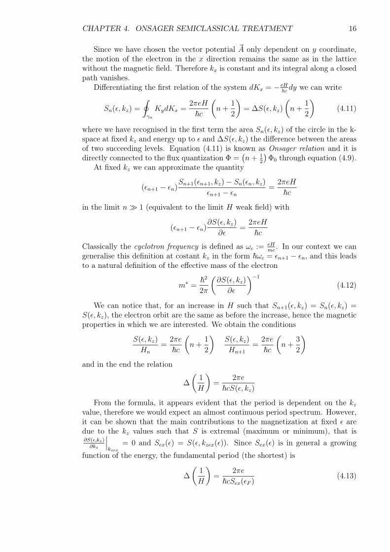
From the formula, it appears evident that the period is dependent on the kzvalue, therefore we would expect an almost continuous period spectrum. However,it can be shown that the main contributions to the magnetization at fixed ϵ aredue to the kz values such that S is extremal (maximum or minimum), that is∂S(ϵ,kz)
∂kz
kzex
= 0 and Sex(ϵ) = S(ϵ, kzex(ϵ)). Since Sex(ϵ) is in general a growing
function of the energy, the fundamental period (the shortest) is
∆
(1
H
)=
2πe
ℏcSex(ϵF )(4.13)
CHAPTER 4. ONSAGER SEMICLASSICAL TREATMENT 17
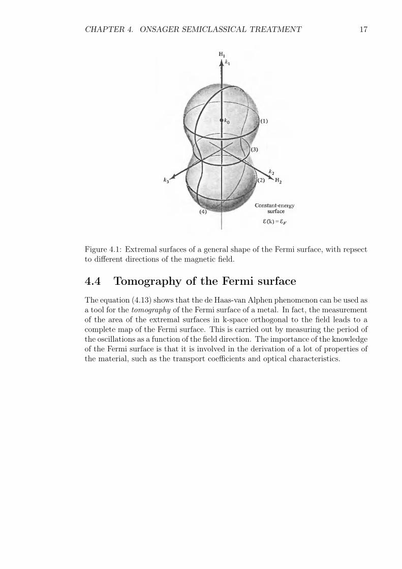
Figure 4.1: Extremal surfaces of a general shape of the Fermi surface, with repsectto different directions of the magnetic field.
4.4 Tomography of the Fermi surfaceThe equation (4.13) shows that the de Haas-van Alphen phenomenon can be used asa tool for the tomography of the Fermi surface of a metal. In fact, the measurementof the area of the extremal surfaces in k-space orthogonal to the field leads to acomplete map of the Fermi surface. This is carried out by measuring the period ofthe oscillations as a function of the field direction. The importance of the knowledgeof the Fermi surface is that it is involved in the derivation of a lot of properties ofthe material, such as the transport coefficients and optical characteristics.
Chapter 5
Quantum treatment
5.1 Landau levelsWe start now with an exact quantum approach of the motion of an electron im-mersed in a magnetic field.
We will take into consideration the presence of the lattice allowing the possi-bility for an effective mass m∗, as already done above. For a matter of simplicityin the following derivations we will exclude the possibility for m∗ to be dependentfrom E, from kz, or from the direction of the magnetic field. In practice, this meansthat m∗ will replace m in every kinetic term, but obviously not in the interactionbetween the intrinsic magnetic moment of the electrons and the magnetic field.This is accurate only for the electrons in the metal which are very weakly boundto atoms’ nuclei and which are near the bottom of a symmetric band, where theenergy may be assumed proportional to k2, and where the Fermi surface is almostspherical.
The general Hamiltonian of such a system is
h =1
2m∗
(p+ e
A(r)
c
)2
− µ · H (5.1)
and introducing the conditions H = (0, 0, H) of uniform field and µ = −2µBSℏ for
the electron, we obtain
h =p2
2m∗ − e
m∗
(2A · p+
[p, A
])+
e2A2
2m∗c2+ 2
µB
ℏSzH
As already done above, we impose the Landau gauge A = (−Hy, 0, 0). Thanks tothe relation
[p, A
]= −iℏ∇ · A = 0, the Hamiltonian becomes
h =1
2m∗
[(px − eH
y
c
)2+ p2y + p2z
]+ 2
µB
ℏSzH
It follows that h, px, pz and Sz are a complete set of commuting observables, theeigenfunctions can be labelled with the quantum numbers kx, kz (whose allowedvalues are all the real numbers) and ms = ±1 and they can be written in the formψkxkzms = ei(kxx+kzz)χms(y).
18
CHAPTER 5. QUANTUM TREATMENT 19
Substituting this expression in the Schrödinger equation hψ = ϵψ together withthe quantities y0 = ℏckx
eHcentre of the armonic oscillator and ωc = eH
m∗ccyclotron
frequency and simplifying the plane wave component, the result is
− ℏ2
2m∗χ′′ms
+m∗ω2
c
2(y − y0)
2χms =
(ϵ− ℏ2k2z
2m∗ −msµBH
)χms (5.2)
This is the equation for a monodimensional harmonic oscillator centred in y0, withangular frequency ωc. Then, it is known that the energy eigenvalues are
ϵkzmsn = ℏωc(n+1
2) +
ℏ2k2z2m∗ +msµBH (5.3)
for n = 0, 1, 2, ... and the eigenfunctions are
χkxkzmsn(y) =1√
2nn!lπ1/4e−
(y−y0)2
2l2 Hn
(y − y0l
)(5.4)
where Hn is the n-th Hermite polinomial and l is the already defined magneticlength. l can be thought as a measure of the localization of the electron, and inthe mentioned experiments, for a magnetic field of 103G and an electron of 2eV ofenergy, it is approximately lt ≈ 5 · 10−3cm.
For what has been said so far, in the Hamiltonian spectrum there are threecomponents: Landau levels (descrete and due to the armonic oscillator), spin-fieldcoupling (descrete) and kinetic energy (continuous and due to the free motion inthe z direction). Since its eigenvalues do not depend on kx, they are infinitely manytimes degenerate.
CHAPTER 5. QUANTUM TREATMENT 20
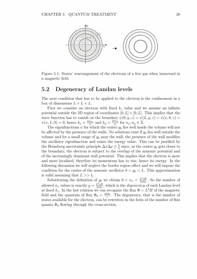
Figure 5.1: States’ rearrangement of the electrons of a free gas when immersed ina magnetic field.
5.2 Degeneracy of Landau levelsThe next condition that has to be applied to the electron is the confinement in abox of dimensions L× L× L.
First we consider an electron with fixed kz value and we assume an infinitepotential outside the 2D region of coordinates [0, L]× [0, L]. This implies that thewave function has to vanish on the boundary ψ(0, y, z) = ψ(L, y, z) = ψ(x, 0, z) =ψ(x, L, 0) = 0, hence kx = 2πnx
Land ky =
2πny
Lfor nx, ny ∈ Z.
The eigenfunctions ψ for which the centre y0 lies well inside the volume will notbe affected by the presence of the walls. No solutions exist if y0 lies well outside thevolume and for a small range of y0 near the wall, the presence of the wall modifiesthe oscillator eigenfunction and raises the energy value. This can be justified bythe Heinsberg uncertainty principle ∆x∆p ≥ ℏ
2since, as the centre y0 gets closer to
the boundary, the electron is subject to the overlap of the armonic potential andof the increasingly dominant wall potential. This implies that the electron is moreand more localised, therefore its momentum has to rise, hence its energy. In thefollowing discussion we will neglect the border region effect and we will impose thecondition for the centre of the armonic oscillator 0 < y0 < L. This approximationis valid assuming that L >> lt.
Substituting the definition of y0 we obtain 0 < nx <L2eH2πℏc . So the number of
allowed nx values is exactly g = L2eH2πℏc , which is the degeneracy of each Landau level
at fixed kz. In the last relation we can recognise the flux Φ = L2H of the magneticfield and the quantum of flux Φ0 = 2πℏc
e. The degeneracy, that is the number of
states available for the electron, can be rewritten in the form of the number of fluxquanta Φ0 flowing through the cross-section.
CHAPTER 5. QUANTUM TREATMENT 21
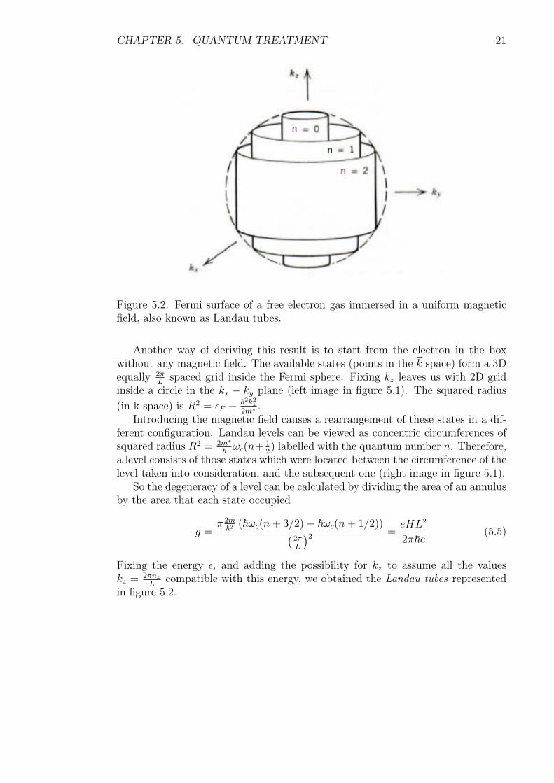
Figure 5.2: Fermi surface of a free electron gas immersed in a uniform magneticfield, also known as Landau tubes.
Another way of deriving this result is to start from the electron in the boxwithout any magnetic field. The available states (points in the k space) form a 3Dequally 2π
Lspaced grid inside the Fermi sphere. Fixing kz leaves us with 2D grid
inside a circle in the kx − ky plane (left image in figure 5.1). The squared radius(in k-space) is R2 = ϵF − ℏ2k2z
2m∗ .Introducing the magnetic field causes a rearrangement of these states in a dif-
ferent configuration. Landau levels can be viewed as concentric circumferences ofsquared radius R2 = 2m∗
ℏ ωc(n+12) labelled with the quantum number n. Therefore,
a level consists of those states which were located between the circumference of thelevel taken into consideration, and the subsequent one (right image in figure 5.1).
So the degeneracy of a level can be calculated by dividing the area of an annulusby the area that each state occupied
g =π 2m
ℏ2 (ℏωc(n+ 3/2)− ℏωc(n+ 1/2))(2πL
)2 =eHL2
2πℏc(5.5)
Fixing the energy ϵ, and adding the possibility for kz to assume all the valueskz =
2πnz
Lcompatible with this energy, we obtained the Landau tubes represented
in figure 5.2.
Chapter 6
Landau’s approach
6.1 Landau’s derivation of diamagnetismNow, we will follow Landau’s original way of deriving the diamagnetism of a freeelectron gas. We consider our system in the limit of weak field H.
First we calculate the spin-field coupling contribution to the magnetic suscep-tibility. The grand canonical potential of a free electron gas is, thanks to therelation (2.11)
Ω0 = − 2
β
∑nx∈Z
∑ny∈Z
∑nz∈Z
ln(1 + e−β( ℏ
2k2
2m∗ −µ))
where the factor 2 is due to the spin degeneracy of each state. Multiplying anddividing by ∆ki = 2π
L, for i = x, y, z we can approximate the last sum with an
integral thanks to the fact that the box considered has L≫ 1. In fact it becomes
Ω0 = − 2
β
(L
2π
)3 ∫ +∞
−∞dkx
∫ +∞
−∞dky
∫ +∞
−∞dkz ln
(1 + e−β( ℏ
2k2
2m∗ −µ))
and changing to spherical coordinates in k space we obtain
Ω0(µ) = − V
βπ
∫ ∞
0
dk ln(1 + e−β( ℏ
2k2
2m∗ −µ))
Including in the Hamiltonian the spin-field coupling contribution cancels the 2factor of the spin degeneracy and makes a translation of the chemical potential,that is
Ωpar =1
2(Ω0(µ− µBH) + Ω0(µ+ µBH))
This leads to a second order H correction
Ωpar = Ω0 +µ2BH
2
2
∂2Ω0
∂µ2+ o(H2)
and a contribution to the magnetic susceptibility
χpar = −µ2B
V
∂2Ω0
∂µ2=µ2B
Vρ(ϵF ) (6.1)
22
CHAPTER 6. LANDAU’S APPROACH 23
where in we have substituted the relation (B.4) of appendix B.2 and we haveidentified ϵF = µ in the limit of T = 0.
On the other hand, including in the Hamiltonian the Landau levels contributionmaintains the spin degeneracy factor and the grand canonical potential, thanks tothe relation (2.11), becomes
Ωdia = − 2
β
+∞∑n=0
∑nz∈Z
eHL2
2πℏcln(1 + e−β(ϵnnz−µ)
)Taking the limit to continuum we can write
Ωdia = − eHV
β2π2ℏc
∞∑n=0
∫ +∞
−∞dkz ln
(1 + e
−β
(ℏ2k2z2m∗ +ℏωc(n+ 1
2)−µ
))
To make this calculation, Landau used the Euler-Maclaurin summation formula
+∞∑n=0
F (n+1
2) ≈
∫ +∞
0
F (x)dx+1
24F ′(0) (6.2)
which is a reasonable approximation in the limit in which F makes a small vari-ation when evaluated in two consecutive Landau levels. This is equivalent to thecondition βℏωc ≪ 1, which will also be assumed in Peierls’ derivation (7.1).
Proceeding we obtain
Ωdia = − eHV
β2π2ℏc
∫ +∞
0
dx
∫ +∞
−∞dkz ln
(1 + e
−β
(ℏ2k2z2m∗ +ℏωcx−µ
))+
− 1
24
eHV
β2π2ℏc
∫ +∞
−∞dkz
−βℏωc
1 + eβ
(ℏ2k2z2m∗ −µ
)
Changing tha variable µ′ → µ − ℏωcx in the first integral makes the first addendindependent from H, so it can be identified with Ω0. The second addend can berecognised as a factor times the second derivative of the first addend with respectto µ.
In particular, using the relations ωc =eHm∗c
and µB = eℏ2mc
we can write
Ωdia = Ω0 −ℏ2ω2
c
24
∂2Ω0
∂µ2= Ω0 −
µ2BH
2
6
( mm∗
)2 ∂2Ω0
∂µ2
and in the end we obtain
χdia = −µ2B
3V
( mm∗
)2 ∂2Ω0
∂µ2= −1
3
( mm∗
)2χpar (6.3)
where we have recognised equation (6.1). χpar can be derived analytically withstandard techniques.
CHAPTER 6. LANDAU’S APPROACH 24
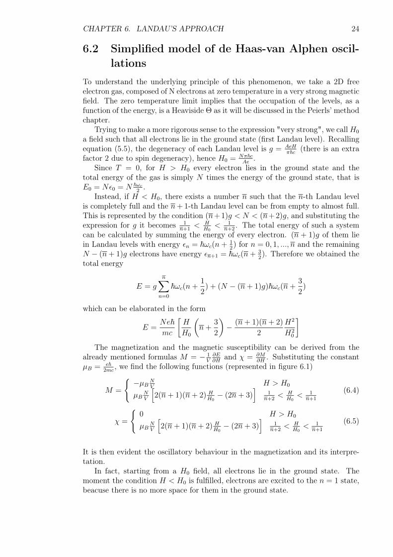
6.2 Simplified model of de Haas-van Alphen oscil-lations
To understand the underlying principle of this phenomenon, we take a 2D freeelectron gas, composed of N electrons at zero temperature in a very strong magneticfield. The zero temperature limit implies that the occupation of the levels, as afunction of the energy, is a Heaviside Θ as it will be discussed in the Peierls’ methodchapter.
Trying to make a more rigorous sense to the expression "very strong", we callH0
a field such that all electrons lie in the ground state (first Landau level). Recallingequation (5.5), the degeneracy of each Landau level is g = AeH
πℏc (there is an extrafactor 2 due to spin degeneracy), hence H0 =
NπℏcAe
.Since T = 0, for H > H0 every electron lies in the ground state and the
total energy of the gas is simply N times the energy of the ground state, that isE0 = Nϵ0 = N ℏωc
2.
Instead, if H < H0, there exists a number n such that the n-th Landau levelis completely full and the n+ 1-th Landau level can be from empty to almost full.This is represented by the condition (n+1)g < N < (n+2)g, and substituting theexpression for g it becomes 1
n+1< H
H0< 1
n+2. The total energy of such a system
can be calculated by summing the energy of every electron. (n + 1)g of them liein Landau levels with energy ϵn = ℏωc(n+ 1
2) for n = 0, 1, ..., n and the remaining
N − (n+ 1)g electrons have energy ϵn+1 = ℏωc(n+ 32). Therefore we obtained the
total energy
E = g
n∑n=0
ℏωc(n+1
2) + (N − (n+ 1)g)ℏωc(n+
3
2)
which can be elaborated in the form
E =Neℏmc
[H
H0
(n+
3
2
)− (n+ 1)(n+ 2)
2
H2
H20
]The magnetization and the magnetic susceptibility can be derived from the
already mentioned formulas M = − 1V
∂E∂H
and χ = ∂M∂H
. Substituting the constantµB = eℏ
2mc, we find the following functions (represented in figure 6.1)
M =
−µB
NV
H > H0
µBNV
[2(n+ 1)(n+ 2) H
H0− (2n+ 3)
]1
n+2< H
H0< 1
n+1
(6.4)
χ =
0 H > H0
µBNV
[2(n+ 1)(n+ 2) H
H0− (2n+ 3)
]1
n+2< H
H0< 1
n+1
(6.5)
It is then evident the oscillatory behaviour in the magnetization and its interpre-tation.
In fact, starting from a H0 field, all electrons lie in the ground state. Themoment the condition H < H0 is fulfilled, electrons are excited to the n = 1 state,beacuse there is no more space for them in the ground state.
CHAPTER 6. LANDAU’S APPROACH 25
Figure 6.1: Magnetization and magnetic susceptibility in an electron gas at T = 0,as functions of the magnetic field strength B. Meccanica Statistica, K. Huang,1997.
So the variation of energy due to the decreasing in the field is composed of 2factor: the energy of each state decreases with the field, but some electrons increasetheir energy moving to the above level. Of these 2 contributions, at the beginningthe excitations of the electrons has a bigger effect and it raises the total energy(negative value of the magnetization), but then the lowering of the energy statestakes over (the magnetization value increases till it becomes positive) and whenalso the second level is filled, the energy is back to the value we started with.
Lowering further the field makes what said above to start over, and it makes themagnetization to quickly change (at T = 0 instantly) from a positive to a negativevalue. M can be viewed as an oscillating function in 1
Hwith period 1
H0.
Chapter 7
Peierls’ method
The following derivations are aimed to describe the motion of the electrons insidea metal immersed in a uniform magnetic field in order to identify some character-istics when the system is under certain conditions. The effects analysed are Pauliparamagnetism, Landau diamagnetism and de Haas-van Alphen oscillations of themagnetization.
The value range for the magnetic field is
ϵF ≫ ℏωc ≫ kBT (7.1)
The physical meaning of this assumption is that there is an almost continuousstructure of Landau levels that electrons can occupy up to the Fermi energy andthat very few electrons occupy energy levels over the Fermi energy, so the statisticof the electrons is almost the one of a Fermi gas (T = 0).
7.1 Mathematics behind the methodTo avoid the difficulty of deriving directly from the definition the grand canonicalpotential, Peierls’ method exploits the relation of this quantity with Boltzmannpartition function, which can be obtained exactly by an analitical calculation.
In particular, considering equation (2.11)
Ω = − 1
β
∑a
ga ln(1 + e−β(ϵa−µ)
)it is useful to call
F (ϵ) := − 1
βln(1 + e−β(ϵ−µ)
)so that Ω =
∑a
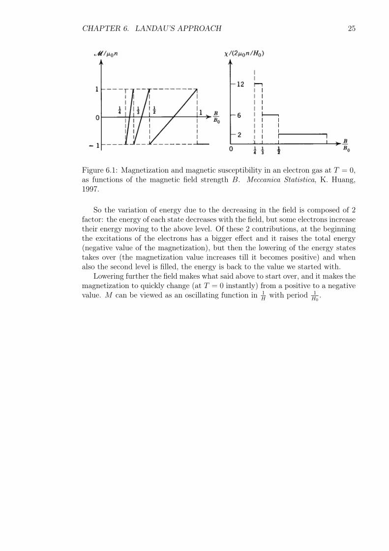
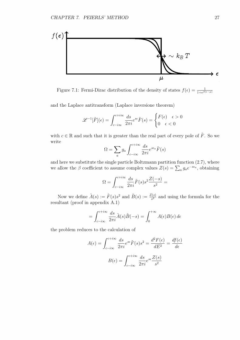
gaF (ϵa) and we can recognise that F (ϵ) is indeed the primitive of
the Fermi-Dirac distribution of the density of states f(ϵ) = 11+eβ(ϵ−µ) represented in
figure 7.1.We denote the Laplace transform of F (ϵ) by
F (s) = L [F ](s) =
∫ +∞
0
e−sϵF (ϵ) dϵ
26
CHAPTER 7. PEIERLS’ METHOD 27
Figure 7.1: Fermi-Dirac distribution of the density of states f(ϵ) = 11+eβ(ϵ−µ)
and the Laplace antitransform (Laplace inversione theorem)
L −1[F ](ϵ) =
∫ c+i∞
c−i∞
ds
2πiesϵF (s) =
F (ϵ) ϵ > 0
0 ϵ < 0
with c ∈ R and such that it is greater than the real part of every pole of F . So wewrite
Ω =∑a
ga
∫ c+i∞
c−i∞
ds
2πiesϵaF (s)
and here we substitute the single particle Boltzmann partition function (2.7), wherewe allow the β coefficient to assume complex values Z(s) =
∑a gae
−sϵa , obtaining
Ω =
∫ c+i∞
c−i∞
ds
2πiF (s)s2
Z(−s)s2
=
Now we define A(s) := F (s)s2 and B(s) := Z(s)s2
and using the formula for theresultant (proof in appendix A.1)
=
∫ c+i∞
c−i∞
ds
2πiA(s)B(−s) =
∫ +∞
0
A(ϵ)B(ϵ) dϵ
the problem reduces to the calculation of
A(ϵ) =
∫ c+i∞
c−i∞
ds
2πiesϵF (s)s2 =
d2F (ϵ)
dE2=df(ϵ)
dϵ
B(ϵ) =
∫ c+i∞
c−i∞
ds
2πiesϵZ(s)
s2
CHAPTER 7. PEIERLS’ METHOD 28
7.2 2D derivation
7.2.1 Boltzmann partition function
The first task is now to obtain explicitly the single particle Boltzmann partitionfunction. Recalling the relation (2.7)
Z =∑a
gae−βϵa =
∑msn
ge−βϵmsn
and the degeneracy of each Landau level (5.5) g = AeH2πℏc , the eigenvalues of the
single particle Hamiltonian are
ϵ = ℏωc(n+1
2) +msµBH (7.2)
Calculating the sum over the quantum numbers
Z =AeH
2πℏc
1∑ms=−1
e−βmsµBH
∞∑n=0
e−βℏωc(n+1/2)
leads toZ(β) =
AeH
2πℏccosh (βµBH)
sinh(βℏωc
2
) (7.3)
Now we substitute Z(s) in the formula for B(E) obtaining
B(ϵ) =AeH
2πℏc
∫ c+i∞
c−i∞
ds
2πi
esϵ
s2cosh (sµBH)
sinh(sℏωc
2
)We change variables into the simpler units z := sℏωc
2and x := 2ϵ
ℏωc, for which z ≫ 1
and x≫ 1 hold because of approximation (7.1), so that it becomes
B =
(AeH
2πℏc
)(ℏωc
2
)I(x) (7.4)
where
I(x) =
∫ c+i∞
c−i∞
dz
2πi
ezx
z2cosh
(zm∗
m
)sinh z
(7.5)
7.2.2 The integral in 2D
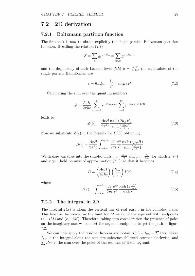
The integral I(x) is along the vertical line of real part c in the complex plane.This line can be viewed as the limit for M → ∞ of the segment with endpoints(c,−iM) and (c,+iM). Therefore, taking into consideration the presence of poleson the imaginary axe, we connect the segment endpoints to get the path in figure7.2.
We can now apply the residue theorem and obtain I(x) + ISC =∑
Res, whereISC is the integral along the semicircumference followed counter clockwise, and∑Res is the sum over the poles of the residues of the integrand.
CHAPTER 7. PEIERLS’ METHOD 29
Figure 7.2: It is represented the path which is followed during the integration.
Beacuse of sinh z term in the denominator, there are infinite simple poles ofthe form nπi for n ∈ Z and because of z2 term, the pole in z = 0 becomes ofthird order. Isc vanishes in the limit of M → ∞, so to evaluate the integral weneed to calculate the sum of the residues. The pole in the origin contribution canbe identified with Pauli paramagnetism and Landau diamagnetism, and the otherpoles contribution with the de Haas-van Alphen effect.
7.2.3 Pauli paramagnetism and Landau diamagnetism
We proceed with the evaluation of
Res
(ezx
z2cosh
(zm∗
m
)sinh z
, z = 0
)Laurent expanding the function in z = 0 and obtaining the residue as the coefficientof the 1
zterm of the serie.
In particular we write
1
z2
(1
z + z3
6+O(z4)
)(1 + xz +
x2z2
2+O(z3)
)(1 +
(m∗)2z2
2m2+O(z3)
)=
=1
z3+x
z2+
1
2z
(x2 +
(m∗
m
)2
− 1
3
)+O(1)
which leads to Resz=0 =12
(x2 +
(m∗
m
)2 − 13
).
CHAPTER 7. PEIERLS’ METHOD 30
A(ϵ) is the derivative of the Fermi-Dirac distribution and in the limit of lowtemperature f(ϵ) → Θ(µ − ϵ), so A(ϵ) → −δ(ϵ − µ), while B(ϵ) is slowly varyingwith the energy, therefore we calculate
Ω = −B(µ) = Ω0 −Am∗
2πℏ2µ2BH
2
(1− 1
3
( mm∗
)2)(7.6)
whereΩ0 = −Am
∗µ2
2πℏ2is the grand canonical potential of a 2D free electron gas (obtained in appendix B.1)and it is H independent.
There is no difference between the chemical potential µ and the Fermi energyϵF of a 2D free electron gas (obtained in appendix B.1). In fact, since the magneticcorrection to the grand canonical potential is independent from µ, imposing theaverage value of the number of electrons N for the free electron gas and for oursystem thanks to the relation N = −∂Ω
∂µ, implies that µ = ϵF . Therefore the
magnetization and the magnetic scusceptibility are
M = µ2BHρ(ϵF )
[1− 1
3
( mm∗
)2](7.7)
χ = µ2Bρ(ϵF )
[1− 1
3
( mm∗
)2](7.8)
where ρ(ϵF ) is the density of states at the Fermi energy for the free electron gas(obtained in appendix B.1).
7.2.4 The de Haas-van Alphen effect
Here we derive the contribution of the poles to grand canonical potential
∑Res =
∑n∈Zn=0
limz→nπi
(z − nπi)ezx cosh
(zm∗
m
)z2 sinh z
=
= −∑n∈Zn=0
limt→nπ
(t− nπ)einπx cos(nπm∗
m)
(nπ)2 sin(t)=
calculating the limit we obtain
= −∑n∈Zn=0
(−)n
(nπ)2einπx cos
(nπ
m∗
m
)=
In the sum only even function contribute, hence
= −2+∞∑n=1
(−)ncos(xnπ)
(nπ)2cos
(m∗
mnπ
)
CHAPTER 7. PEIERLS’ METHOD 31
In this case, we can not approximate A(ϵ) with the Dirac delta function sinceB(ϵ) is a quickly varying function with respect to the energy, so we have to calculatethe integral before taking the low temperature limit. In particular
Ω =
(βAeH
4πℏc
)(ℏωc
2
) +∞∑n=1
(−)ncos(m
∗
mnπ)
(nπ)2
∫ +∞
0
dϵcos(
nπ2ϵℏωc
)cosh2
(β ϵ−µ
2
)Making the substitution t := β ϵ−µ
2allow us to recognise a known integral and
to clarify what is involved in the limit T → 0. So we obtain
Ω =
(AeH
2πℏc
)(ℏωc
2
) +∞∑n=1
(−)ncos(m
∗
mnπ)
(nπ)2cos
(2nπµ
ℏωc
)J
where J is the following integral (calculated in appendix A.3)
J =
∫ +∞
−βµ2
dtcos(
4nπβℏωc
t)
cosh2 t=
4nπ2
βℏωc
1
sinh(
2π2nβℏωc
)where, since µ ≫ kBT thanks to the approximation (7.1), we have extended theintegral till −∞. In the end we elaborate the grand canonical potential in the form
Ω =AeH
πℏcβ
+∞∑n=1
(−)n
ncos
(nπ
m∗
m
) cos(
2nπµℏωc
)sinh
(2nπ2
βℏωc
) (7.9)
It appears evident that the magnetization can be viewed as an oscillating func-tion of the variable 1
Hwith fundamental (shortest) period ∆
(1H
)= eℏ
ϵFm∗c. This
result is coherent with the simplified (T = 0) derivation already done, where wefound ∆
(1H
)= 1
H0= Ae
Nπℏc . These 2 expression coincide if we substitute N = m∗ϵFAπℏ2
the number of electrons for a T = 0 electron gas.
CHAPTER 7. PEIERLS’ METHOD 32
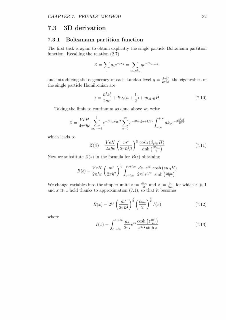
7.3 3D derivation
7.3.1 Boltzmann partition function
The first task is again to obtain explicitly the single particle Boltzmann partitionfunction. Recalling the relation (2.7)
Z =∑a
gae−βϵa =
∑msnkz
ge−βϵmsnkz
and introducing the degeneracy of each Landau level g = AeH2πℏc , the eigenvalues of
the single particle Hamiltonian are
ϵ =ℏ2k2z2m∗ + ℏωc(n+
1
2) +msµBH (7.10)
Taking the limit to continuum as done above we write
Z =V eH
4π2ℏc
1∑ms=−1
e−βmsµBH
∞∑n=0
e−βℏωc(n+1/2)
∫ +∞
−∞dkze
−βℏ2k2z2m∗
which leads to
Z(β) =V eH
2πℏc
(m∗
2πℏ2β
) 12 cosh (βµBH)
sinh(βℏωc
2
) (7.11)
Now we substitute Z(s) in the formula for B(ϵ) obtaining
B(ϵ) =V eH
2πℏc
(m∗
2πℏ2
) 12∫ c+i∞
c−i∞
ds
2πi
esϵ
s3/2cosh (sµBH)
sinh(sℏωc
2
)We change variables into the simpler units z := sℏωc
2and x := 2ϵ
ℏωc, for which z ≫ 1
and x≫ 1 hold thanks to approximation (7.1), so that it becomes
B(x) = 2V
(m∗
2πℏ2
) 32(ℏωc
2
) 52
I(x) (7.12)
where
I(x) =
∫ c+i∞
c−i∞
dz
2πiezx
cosh(zm∗
m
)z5/2 sinh z
(7.13)
CHAPTER 7. PEIERLS’ METHOD 33
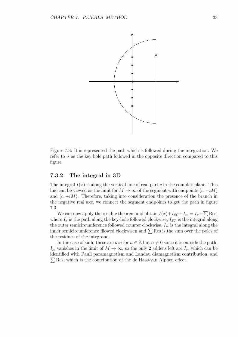
Figure 7.3: It is represented the path which is followed during the integration. Werefer to σ as the key hole path followed in the opposite direction compared to thisfigure
7.3.2 The integral in 3D
The integral I(x) is along the vertical line of real part c in the complex plane. Thisline can be viewed as the limit for M → ∞ of the segment with endpoints (c,−iM)and (c,+iM). Therefore, taking into consideration the presence of the branch inthe negative real axe, we connect the segment endpoints to get the path in figure7.3.
We can now apply the residue theorem and obtain I(x)+ISC+Isc = Iσ+∑
Res,where Iσ is the path along the key-hole followed clockwise, ISC is the integral alongthe outer semicircumference followed counter clockwise, Isc is the integral along theinner semicircumference fllowed clockwisen and
∑Res is the sum over the poles of
the residues of the integrand.In the case of sinh, these are nπi for n ∈ Z but n = 0 since it is outside the path.
Isc vanishes in the limit of M → ∞, so the only 2 addens left are Iσ, which can beidentified with Pauli paramagnetism and Landau diamagnetism contribution, and∑
Res, which is the contribution of the de Haas-van Alphen effect.
CHAPTER 7. PEIERLS’ METHOD 34
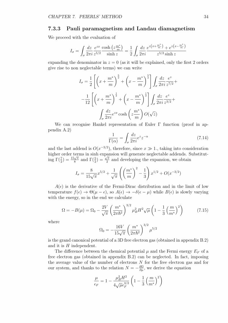
7.3.3 Pauli paramagnetism and Landau diamagnetism
We proceed with the evaluation of
Iσ =
∫σ
dz
2πi
ezx
z5/2cosh
(zm∗
m
)sinh z
=1
2
∫σ
dz
2πi
ez(x+m∗m ) + ez(x−
m∗m )
z5/2 sinh z
expanding the denominator in z = 0 (as it will be explained, only the first 2 ordersgive rise to non neglectable terms) we can write
Iσ =1
2
[(x+
m∗
m
) 52
+
(x− m∗
m
) 52
]∫σ
dz
2πi
ez
z7/2+
− 1
12
[(x+
m∗
m
) 12
+
(x− m∗
m
) 12
]∫σ
dz
2πi
ez
z3/2+
∫σ
dz
2πiezx cosh
(zm∗
m
)O(
√z)
We can recognise Hankel representation of Euler Γ function (proof in ap-pendix A.2)
1
Γ(α)=
∫σ
dz
2πiezz−α (7.14)
and the last addend is O(x−3/2), therefore, since x≫ 1., taking into considerationhigher order terms in sinh expansion will generate neglectable addends. Substitut-ing Γ(7
2) = 15
√π
8and Γ(5
2) =
√π2
and developing the expansion, we obtain
Iσ =8
15√πx5/2 +
1√π
((m∗
m
)2
− 1
3
)x1/2 +O(x−3/2)
A(ϵ) is the derivative of the Fermi-Dirac distribution and in the limit of lowtemperature f(ϵ) → Θ(µ − ϵ), so A(ϵ) → −δ(ϵ − µ) while B(ϵ) is slowly varyingwith the energy, so in the end we calculate
Ω = −B(µ) = Ω0 −2V√π
(m∗
2πℏ2
)3/2
µ2BH
2√µ(1− 1
3
( mm∗
)2)(7.15)
where
Ω0 = − 16V
15√π
(m∗
2πℏ2
)3/2
µ5/2
is the grand canonical potential of a 3D free electron gas (obtained in appendix B.2)and it is H independent.
The difference between the chemical potential µ and the Fermi energy EF of afree electron gas (obtained in appendix B.2) can be neglected. In fact, imposingthe average value of the number of electrons N for the free electron gas and forour system, and thanks to the relation N = −∂Ω
∂µ, we derive the equation
µ
ϵF= 1− µ2
BH2
4√µϵ
3/2F
(1− 1
3
( mm∗
)2)
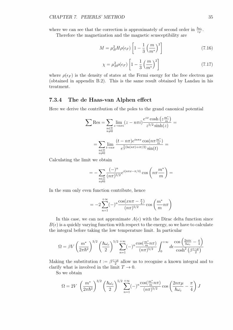
CHAPTER 7. PEIERLS’ METHOD 35
where we can see that the correction is approximately of second order in ℏωc
ϵF.
Therefore the magnetization and the magnetic scusceptibility are
M = µ2BHρ(ϵF )
[1− 1
3
( mm∗
)2](7.16)
χ = µ2Bρ(ϵF )
[1− 1
3
( mm∗
)2](7.17)
where ρ(ϵF ) is the density of states at the Fermi energy for the free electron gas(obtained in appendix B.2). This is the same result obtained by Landau in histreatment.
7.3.4 The de Haas-van Alphen effect
Here we derive the contribution of the poles to the grand canonical potential
∑Res =
∑n∈Zn=0
limz→nπi
(z − nπi)ezx cosh
(zm∗
m
)z5/2 sinh(z)
=
=∑n∈Zn=0
limt→nπ
(t− nπ)einπx cos(nπm∗
m)
e52(ln(nπ)+iπ/2) sin(t)
=
Calculating the limit we obtain
= −∑n∈Zn=0
(−)n
(nπ)5/2ei(nπx−π/4) cos
(nπ
m∗
m
)=
In the sum only even function contribute, hence
= −2+∞∑n=1
(−)ncos(xnπ − π
4)
(nπ)5/2cos
(m∗
mnπ
)In this case, we can not approximate A(ϵ) with the Dirac delta function since
B(ϵ) is a quickly varying function with respect to the energy, so we have to calculatethe integral before taking the low temperature limit. In particular
Ω = βV
(m∗
2πℏ2
)3/2(ℏωc
2
)5/2 +∞∑n=1
(−)ncos(m
∗
mnπ)
(nπ)5/2
∫ +∞
0
dϵcos(
2nπϵℏωc
− π4
)cosh2
(β ϵ−µ
2
)Making the substitution t := β ϵ−µ
2allow us to recognise a known integral and to
clarify what is involved in the limit T → 0.So we obtain
Ω = 2V
(m∗
2πℏ2
)3/2(ℏωc
2
)5/2 +∞∑n=1
(−)ncos(m
∗
mnπ)
(nπ)5/2cos
(2nπµ
ℏωc
− π
4
)J
CHAPTER 7. PEIERLS’ METHOD 36
where J is the following integral (calculated in appendix A.3)
J =
∫ +∞
−βµ2
dtcos(
4nπβℏωc
t)
cosh2 t=
4nπ2
βℏωc
1
sinh(
2π2nβℏωc
)where, since µ ≫ kBT , we have extended the integral till −∞. In the end weelaborate the grand canonical potential in the form
Ω =V
2π2β
(eH
ℏc
)3/2 +∞∑n=1
(−)n
n3/2cos
(nπ
m∗
m
) cos(
2nπµℏωc
− π4
)sinh
(2π2nβℏωc
) (7.18)
7.4 Comparing semiclassical and quantum resultsIn the limit (7.1), we can identify µ with the ϵF of a free electron gas and it appearsevident that the magnetization, both in 2D e 3D, oscillates as a function of 1
Hwith
fundamental period ∆(
1H
)= eℏ
m∗cϵF. This result is coherent with the semiclassical
one (4.13) ∆(
1H
)= 2πe
ℏcSex(ϵF ).
Thanks to Onsager relation (4.11) Sn(ϵ, kz) = ∆S(ϵ, kz)(n+ 1
2
), there exist an
n such that Sex(ϵF ) = ∆Sex(ϵF )(n+ 1
2
). We can now approximate ∆Sex(ϵF ) ∼=
∂Sex(ϵ)∂ϵ
ϵ=ϵF
∆ϵ where, since our Fermi surface is assumed to be almost spherical we
obtain kzex = 0, hence ∆ϵ = ℏωc and ϵF =(n+ 1
2
)∆ϵ.
Therefore, the relation we obtain is Sex(ϵF ) =∂Sex(ϵ)
∂ϵ
ϵ=ϵF
ϵF where, in the par-
tial derivative, we can recognise the definition of the effective mass m∗(ϵF , kzex) =ℏ22π
∂Sex(ϵ)∂ϵ
ϵ=ϵF
, evaluated at ϵF and kzex.Making this substitution, the 2 periods coincide. The semiclassical period is
more general than the one found by Peierls’ method for an almost free electron gas,since it can take into account not only ellipsoid Fermi surfaces, but very differentshapes.
Appendix A
A.1 Proof of the resultant formulaHere we provide a proof to the resultant formula, which is∫ c+i∞
c−i∞
ds
2πiA(s)B(−s)esx =
∫ +∞
max(0,x)
dϵA(ϵ)B(ϵ− x) (A.1)
where A(s) = L [A](s) and B(s) = L [B](s).Replacing B(s) with the definition of the Laplace transform we obtain for the
first term∫ c+i∞
c−i∞
ds
2πiA(s)esx
∫ +∞
0
dy B(y)esy =
∫ c+i∞
c−i∞
ds
2πi
∫ +∞
0
dyB(y)A(s)es(x+y)
We can now interchange the integrals and recognise the Laplace antitrasform ofA(s) and substitute it∫ +∞
0
dy B(y)
∫ c+i∞
c−i∞
ds
2πiA(s)es(y+x) =
∫ +∞
0
dy B(y)A(y + x)Θ(y + x)
which gives the expressione above after the variable change E := x+ y.
A.2 Hankel representation of Euler Γ functionHere we provide a proof to the formula known as Hankel representation of Euler γfunction
1
Γ(α)=
∫σ
dz
2πiezz−α = (A.2)
We choose the convention for the logarithm discontinuity at the negative part ofthe real axis (principal logarithm).
Therefore we can write more explicity
= limϵ→0
∫ iϵ
−∞−iϵ
dz
2πi
ez
eα(ln |z|+i arg z)+
∫ −∞+iϵ
iϵ
dz
2πi
ez
eα(ln |z|+i arg z)=
With the convention chosen, we obtain that arg z = −π and arg z = π respectivelyin the first and in the second integral. Changing the variable with t := −z ± iϵ
37
APPENDIX A. 38
and calculating the limit, we obtain
=
∫ +∞
0
dy
2πi
e−y
yα(eiαπ − e−iαπ
)=
sin(απ)
π
∫ +∞
0
dy e−yy−α =
In the last term we can recognise the definition of Euler’s Γ function, and inthe end the expression becomes
=sin(απ)
πΓ(1− α) =
1
Γ(α)
where the last equal sign is due to Euler’s reflection formula, which is valid if α /∈ Z.In the present case α = n
2where n is an odd integer, so no domain problems arise.
A.3 The integral of cos(αt)
cosh2(t)
In the calculations above we encountered an integral of the form
I(α) =
∫ +∞
−∞dt
cos(αt)
cosh2(t)(A.3)
which can be also calculated thanks to the residue theorem. We can write theintegral above as the limit for M → ∞ of the integral along the segment [−M,M ]on the real axe, allowing the variable t to take also complex values.
We close this segment creating a rectangle of vertices −M , M , M+iπ, −M+iπ.This path sorrounds the t = iπ/2 second order pole due to the denominator.The integrals along the vertical segments vanish in the M → ∞ limit becausethe numerator of the integrand is a limited quantity meanwhile the denominatordiverges.
So we obtain
limM→∞
IM(α) +
∫ −M
M
dtcos(α(t+ iπ))
cosh2(t+ iπ)= 2πiRes
(cos(αt)
cosh2(t),iπ
2
)=
In the second addend of the first term of the equation above, we can recognise− cosh(απ)IM(α) and the residue can be calculated as follows
= 2πi limt→iπ/2
d
dt
((t− iπ
2
)2cos(αt)
cosh2(t)
)= −2πα sinh
(απ
2
)which becomes the value above after some algebra.
In the end it results
I(α) =−2πα sinh
(απ
2
)1− cosh(απ)
=πα
sinh(απ
2
)
Appendix B
The free electron gas
B.1 2D calculationsIn this appendix we aim to calculate the grand partition function Ω0 of a 2D freeelectron gas at T = 0 using Peierls’ method. So the single particle energy is ϵ = ℏ2k2
2m∗
and the canonical partition function is Z(β) = gs∑kxky
e−βϵkxky , where gs = 2 is the
spin degeneracy of each electron.The electrons are confined in L × L box, so imposing the period boundary
conditions we obtain kj =2πnj
Lwhere j = x, y and nj ∈ Z. The number of
states in the annulus 2πkdk is 2 2πkdk
( 2πL )
2 , so the density of states per unit area in
k space is ρ(k) = Akπ
and the denisty of states as a function of the energy isρ(ϵ) = ρ(k)dk
dϵ= Am∗
πℏ2 .To calculate the partition function, we take the limit to the continuum and we
change to polar coordinates in the k space, so that we can write the sum as theintegral
Z(β) =A
2π2
∫ +∞
0
dk 2πke−β ℏ2k22m∗ =
Am∗
πℏ2β(B.1)
In the limit of low temperature, as already explained, we can derive Ω0 = −B(µ),where
B(ϵ) =
∫ c+i∞
c−i∞
ds
2πiesϵZ(s)
s2=Am∗
πℏ2
∫ c+i∞
c−i∞
ds
2πi
esϵ
s3
As done in the H = 0 case, we can write the integral above I0 as a part of theintegral along the path in figure 7.2. Here there is only one third order pole s = 0inside the path, so we can simply calculate its residue from the Laurent expansionesϵ
s3= 1
s3+ ϵ
s2+ ϵ2
2s+O(1) which leads to I0 = ϵ2
2and in the end we obtain
Ω0 = −Am∗
2πℏ2µ2 (B.2)
B.2 3D calculationsIn this appendix we aim to calculate the grand partition function Ω0 of a 3D freeelectron gas at T = 0 using Peierls’ method. So the single particle energy is ϵ = ℏ2k2
2m∗
39
APPENDIX B. THE FREE ELECTRON GAS 40
and the canonical partition function is Z(β) = gs∑
kxkykz
e−βϵkxkykz , where gs = 2 is
the spin degeneracy of each electron.The electrons are confined in L×L×L box, so imposing the period boundary
conditions we obtain kj =2πnj
Lwhere j = x, y, z and nj ∈ Z. The number of states
in the spherical shell 4πk2dk is 24πk2dk
( 2πL )
3 , so the density of states per unit volume
in k space is ρ(k) = V k2
π2 and the denisty of states as a function of the energy isρ(E) = ρ(k) dk
dE=
√2V (m∗)3/2
√E
π2ℏ3 .To calculate the partition function, we take the limit to the continuum and we
change to spherical coordinates in the k space, so that we can write the sum as theintegral
Z(β) =V
π2
∫ +∞
0
dk k2e−β ℏ2k22m∗ = 2V
(m∗
2πℏ2β
) 32
(B.3)
In the limit of low temperature, as already explained, we can derive Ω0 = −B(µ)where
B(ϵ) =
∫ c+i∞
c−i∞
ds
2πiesϵZ(s)
s2= 2V
(m∗
2πℏ2
) 32∫ c+i∞
c−i∞
ds
2πi
esϵ
s7/2
As done in the H = 0 case, we can write the integral above I0 as a part of theintegral along the path in figure 7.3. Here there are no poles inside the path so wecan simply calculate
I0 =
∫σ
ds
2πi
esϵ
s7/2=
ϵ5/2
Γ(72
)In the end we obtain
Ω0 = −B(µ) = − 16
15√πV
(m∗
2πℏ2
) 32
µ5/2 (B.4)
Bibliography
[1] W. J. de Haas, P. M. van Alphen, The dependence of the susceptibility of dia-magnetic metals upon the field, Communication NO. 212a from the PhysicalLaboratory, Leiden (1930).
[2] M. Blackman, On the diamagnetic susceptibility of bismuth, Trinity College,Cambridge (1938).
[3] D. Schoenberg, The de Haas-van Alphen effect, Royal Society Mond Laboratory,University of Cambridge (1951).
[4] K. Huang, Meccanica Statistica, Zanichelli (1997).
[5] J. P. Sethna, Statistical Mechanics, Entropy, Order Parameters, and Complex-ity, Clarendon Press (2017).
[6] R. E. Peierls, Quantum Theory of Solids, Oxford University Press (2001).
[7] J. H. Van Vleck, The Theory of Electric and Magnetic Susceptibilities, OxfordUniversity Press (1932).
[8] L. D. Landau, E. M. Lifshitz, Fisica Teorica 3, Meccanica Quantistica, Teorianon relativistica, Editori Riuniti (1986).
[9] L. D. Landau, E. M. Lifshitz, Fisica Teorica 5, Fisica Statistica, Parte prima,Editori Riuniti (1986).
[10] L. D. Landau, E. M. Lifshitz, Fisica Teorica 9, Fisica Statistica, Parte sec-onda, Teoria dello Stato Condensato, Editori Riuniti (1986).
[11] J. J. Quinn, K. S. Yi, ,Solid State Physics, Principles and Modern Applica-tions, Springer (2018).
[12] N. W. Ashcroft, N. D. Mermin, Solid State Physics, Harcourt College Pub-lishers (1976).
[13] L. D. Landau, Diamagnetismus der Metalle, Zeitschrift für Physik 64 , 629(1930).
[14] S. Blundell, Magnetism in Condensed Matter, Oxford University Press (2001).
[15] D. Shoenberg, Magnetic oscillations in metals, Cambridge University Press(1984).
41
BIBLIOGRAPHY 42
[16] E. H. Sondheimer, A. H. Wilson, The diamagnetism of free electrons, TrinityCollege, Cambridge (1951).
[17] L. G. Molinari, Notes on Magnetism in Noninteracting Electron Gas, http://wwwteor.mi.infn.it/~molinari/NOTES/wilson2019.pdf, (2007).
[18] L. G. Molinari, Mathematical Methods for Physics, CUSL (2019).
[19] M. R. Spiegel, Teoria ed Applicazioni delle Trasformate di Laplace, GruppoEditoriale Frabbri (1976).