Inter-American Development Bank

Banco Interamericano de Desarrollo Banco Interamericano de desenvolvimento Banque interámericaine de développement

Working Paper CSI-164

Land Titles and Conflicts in Guatemala

by

Karen Macours

School of Advanced International Studies, Johns Hopkins University

March 2009

2

Abstract1 This paper analyzes the impact of formal property rights on plot use and credit access in 20 communities in Guatemala, and shows how these impacts differ depending on the community conflict context. The paper proposes a new instrument based on detailed information about the geographic location of the plots and historical titling processes to address the endogeneity concerns that are common in the property rights literature. The paper sheds light on whether the effect of land titles on plot use and credit access varies with the prevalence of conflicts and different types of conflict resolution mechanisms. The findings suggest that these factors might be crucial to understand the potential impacts on plot use of possible titling programs. Keywords: Land titling, Conflicts, Latin America JEL Classifications: O12, O13

1 This paper has benefited from comments by Steve Boucher, Michael Carter, Suzanne Duryea, Nestor Gandelmann, Hugo Ñopo, Ernesto Schargrodsky, Eduardo Zegarra, and participants at the LACEA 2007 conference. Jonathan Bartalozzi and Smriti Lakhey provided excellent research assistance. Financial support from the IADB and USAID is gratefully acknowledged. All errors are my own. Author contact information: International Economics, School of Advanced International Studies (SAIS) Johns Hopkins University, 1717 Massachusetts Avenue N.W., Washington DC 20036; Tel 202 663 5679; Fax 202 663 7718; kmacours@jhu.edu

3

1. Introduction The recent empirical growth literature emphasizes property rights as the prime example of how

institutions can affect growth (Acemoglu, Johnson, and Robinson, 2001; Acemoglu and Johnson,

2005). Theoretically, there are indeed a number of reasons why property rights security would

have a positive effect on efficiency, and these reasons are often used to motivate land titling

programs. Formal titles are believed to increase the incentives for investments, facilitate access

to credit by providing collateral, and guarantee allocative efficiency by facilitating land market

transactions.

The micro-evidence regarding these effects, however, is mixed. Besley (1995) finds that

property rights increase plot investments in one region, but not another, and Braselle, Gaspart

and Platteau (2002) find that the lack of property rights can in fact increase investment in the

form of tree planting. Focusing more specifically on the effects of land titling in Latin America,

Field (2005), Galiani and Schargrodsky (2006), and Di Tella, Galiani and Schargrodsky (2007)

find effects on labor supply, housing investments, and beliefs, but not on credit, in urban

squatting settings in Peru and Argentina. Moreover, Lanjouw and Levy (2002) find that formal

and informal rights might be substitutable in urban Ecuador.

The evidence for rural settings in Latin America is also mixed. Carter and Olinto (2003)

and Boucher, Barham and Carter (2005) find that the effects of formal titling might be limited in

the presence of other market imperfections. Finally, Macours, de Janvry and Sadoulet (2007)

find that informal property rights and conflict affect land allocation, while not finding an effect

of formal titles.

Different reasons might help explain why the empirical evidence on the issue is mixed.

First of all, all these studies need to make certain assumptions about the exogeneity of the titling

status, or about the instruments used to identify the effects of titles, and the findings hence rely

on those assumptions. But even when identification issues are resolved, it is not unlikely that the

effect of titles crucially depends on several other factors that affect household decision-making,

as many of the authors above have discussed. These can be factors that are specific to the

household, or factors related to the community or general context in which they live. In

particular, given that we expect titles to have an effect because they help guarantee security of

property rights, their effect might well depend on other factors that also determine security of

4

property rights, such as the general rule of law in a country, the local history of conflicts, or

existing conflict resolution mechanisms.

This paper contributes to this literature by proposing a new instrument to address

endogeneity concerns and by focusing on the interaction between titles and the community

conflict context. Specifically, this paper attempts to shed light on whether the effect of land titles

on plot use and credit access varies with the prevalence of conflicts and different types of

conflict resolution mechanisms. The identification strategy relies on the fact that most formal

titles were granted at the end of the nineteenth century. At that point, the applications for titling

were made simultaneously for large tracts of land, either by individuals or by community leaders.

While much of this land was subsequently fragmentized among many owners, the title status of

different plots is still correlated.

This paper is motivated by the combination of widespread property rights insecurity and

long-standing land conflicts that characterize large parts of rural Guatemala. Property rights

insecurity in Guatemala results in part from the massive lack of formal land titles, and

understanding the interaction between titles and land conflicts might be crucial to shed light on

the potential pay-offs of titling programs. The question this paper addresses is hence important

for its possible implications and might entail lessons for both targeting and the potential need for

complementary programs focusing on conflict resolution mechanisms. Given that the prevalence

of land conflicts clearly is not unique to Guatemala, this is likely to be of broader relevance for

policymakers in Latin America.

The structure of the paper is as follows. In the next section, we provide more background

on the historical processes that shed light on titling variation and land conflicts in Guatemala. In

Section 3, we discuss the data and the outcome variables. Section 4 discusses the identification

strategy, and Section 5 presents the results on the relationship between titles and several plot and

household level outcomes. Section 6 then discusses how the effect of titles can be better

understood once the local conflict context is taken into account. Finally, Section 7 concludes.

5

2. Background on Titles and Conflict In Guatemala, most existing titles go back to the end of the nineteenth century when, because of

the coffee boom, the government encouraged the transformation from community to private

property. Such transformations required an application by individual owners and/or local

authorities. In areas where cultural values related to common ownership were strong and no

internal conflicts or outside speculators arose, the people occupying the land would not apply for

title. Over time, these communities moved from common to individual ownership but without

establishing formal title. Some other long-term owners, however, lost (part of) their land as a

result of false applications and/or land invasions by outsiders, who were often ladino. However,

not all of the new owners obtained a formal title. Overall, the fate of a plot of land (in terms of

land titling and access) depended on a village’s location and population, and on how quickly

local leaders came to understand the new situation (McCreery, 1994; Grandin, 2000). Within a

community as well, though, much variation in titling resulted because land that was of higher

quality was more likely to be claimed and titled by outside parties, possibly because of false

applications by outsiders, while lack of knowledge on the part of some long-term possessors also

affected title status. Also, in some cases, outsiders managed to claim only part of a larger parcel

(Naylor, 1967). The title status today is to a large extent driven by these historical events. While

there have been various organized titling efforts by the government since the 1960s, these

activities were concentrated on settlements and titling on frontier lands in the Peten, a

department in the North of the country that is not part of our study. Hence in many communities,

some tracts of land are titled while other tracts within the same community are not.

Lack of formal titles affects land allocation decisions in part because of legislation that

allows registering an untitled plot of land in the public property registry after 10 years of

peaceful and undisputed possession (the Ley de Titulación Supletoria). Although in principle this

law should only apply to land that satisfies a very narrow set of criteria, it leaves room for false

declarations, abuses and corruption, and as such has been a source of de facto property rights

insecurity in the land market (Chang, 2002).

Property rights insecurity is reinforced by long-standing tensions regarding access to

land. Unequal distribution of land, resulting from perceived historical injustices during the

colonization and early post-colonization eras, has been recognized as one of the causes

underlying the violent civil conflict of the 1980s. At the local level, conflicts over land are

6

extremely common and range from trespassing to squatting, inheritance-related conflicts and

conflicts over common property resources. Widespread lack of confidence and trust in the

national juridical system often impedes conflict resolution (Chang, 2002). Many indigenous

communities have their own local mechanisms for conflict resolution. However, these

mechanisms might be limited in their capacity to solve problems with people that do not live in

the community. As a result, many conflicts linger for years.

3. Data and Outcome Variables This paper relies on a micro-level dataset of 20 communities in 2 regions (Alta Verapaz and

Quetzaltenango) in Guatemala. Alta Verapaz is a department in the Northeast of the country

where communities of peasants border to estates of large landowners. Quetzaltenango, is a

department in the central highlands, and most of the households in the sampled communities are

mini-fundistas (see also Macours, 2007). Data on all households living in the communities (1,822

in total) and on all their plots were obtained from interviews with a key informant in each

community. Households with a secondary residence in the community were also included (these

are mostly large landowners who do not necessarily live year-round on their estate). In addition

to the usual plot and household-level characteristics, the geographic location of all plots was

identified by drawing plot-level village maps. Furthermore, extensive information about conflicts

and conflict resolution mechanisms was collected at the plot, household and community level.2

Key informants, typically community leaders, were selected based on their knowledge of

all households and their activities in the land market.3 The data collection relied on the use of key

informants, instead of direct interviews with the household head, because the topic of land and

land conflicts is extremely sensitive in Guatemala. Working with selected key informants hence

prevented problems of misreporting or refusals to participation in the survey by individual

households, which had been observed when land-related questions were asked in previous

(unrelated) survey efforts in Guatemala. In Macours (2003), the answers of key respondents are

compared with answers from households themselves for a related questionnaire in the Dominican

2 Communities are geographical units (i.e., villages), typically consisting of a nucleus of houses and some more dispersed dwellings, and they were defined using existing contemporary boundaries. As such, communities differ from the historic comunidades indígenas that largely correspond to the current municipalities. The number of households in a community varies between 17 and 173. 3 This selection was made based on discussions with various community members, in which the type of information that would be asked for was explained.

7

Republic. The level of agreement between the two types of respondents on questions regarding

households’ assets holding, demographics, and land use was found to be relatively large.4

Table 1A reports a number of key individual and household characteristics of both the

key informants, and of the landowning households in the sample.5 Compared to the average

household, the key informants have all lived in the community since birth, tend to have more

family in the community, and are somewhat more likely to be from the majority indigenous

group, more likely to be literate, and less likely to have either a high or a low livings standard.6

All these characteristics are consistent with their leadership position in the communities. On the

other hand, they appear to own less land, which mainly captures the fact that among the other

households, there are a few large landowners that skew the distribution. Overall, the key

informants do not seem extremely different from the average household in the community. In the

analysis, we will test whether some of the differences between informants and households affect

the findings.

To obtain the main independent variable, informants were asked whether there was a

title, registered in the public registry, for each plot owned by the households in the community.

Many of these titles might be outdated, and informants might not know whether titles are

updated or not. Our independent variable only measures whether the plot has a formal title,

registered in the public registry, not whether it is in name of the current owner.

Furthermore, while key informants are unlikely to have accurate information about plot

yields or detailed input use, they do have a comparative perspective on how efficiently different

plots are used in their community. They were asked therefore to evaluate whether each plot was

used according to its potential or was being under-used.7 This will be used as our first plot-level

outcome variable of interest. A second variable captures information about actual use of the plot.

4 The use of key informants to obtain information about other households in a community is most common in Rapid Rural Appraisal (RRA) exercises. While for RRA key informants are usually asked to provide rankings of households, Takasaki, Barham and Coomes (2000) have explored the possibility of collecting data on asset ownership from key informants. The approach discussed in this paper is related to theirs. 5 Landless households are not part of the analysis in this paper. 6 Informants were asked to classify each household according to their living standards. At the beginning of each interview, guidelines were established regarding how to evaluate income levels, and informants were asked to consider the conditions of the house, material it was build from, consumption and health levels, and access to services in their evaluation. They were specifically instructed not to take the productive potential of the households into account in this evaluation. The analysis in Macours (2003) shows that a similar approach leads to welfare variables that were highly correlated with reports of living conditions by households themselves. 7 The estimations exclude all small parcels (less than two cuerdas or about 0.09 hectares) that are used exclusively for housing.

8

It particular, it indicates whether the plot is being used for pasture, forest, or lies idle, which are

all more extensive uses of the land (compared to commercial crops, corn, etc.).8 The indicators

of the efficiency of use and of extensive use will allow us to test the relationship between titles

and plot-level productivity and investment. To evaluate the overall relationship between titles

and credit access, informants were asked whether the household would be able to obtain formal

credit. When discussing the empirical results, we will return to the interpretation of the findings

regarding credit access, taking into account that the information was obtained through the key

informant.

While clearly informants’ responses to these questions will have measurement error, this

will not bias the results as long as it is not systematically related to the independent variable. All

the questions about outcome variables were asked before the plot’s title status was discussed in

order to minimize bias. Moreover, in the empirical estimations, we control for community fixed

effects, which will eliminate any systematic informant bias that is constant across households of

one community. As such, our outcome variables indicate plot and household outcomes relative to

the rest of the community.9 More generally, we conduct a number of checks to test the robustness

of the results for the assumptions underlying the use of the key informant (discussed below).

Table 1B shows the means of the three outcome variables by title status of the plots, as

well as an indicator of overall household welfare. As indicated in the table, 22 percent of the

plots in the sample have formal registered titles, and these plots are more likely to be efficiently

used, and less likely to be used extensively. Owners of such plots are more likely to have a

higher living standard and are more likely to have access to credit. Yet, in order to determine

whether the observed relationship between titles and these outcome variables are causal, we

clearly need to account for the possible endogeneity of the title status, as will be discussed

below.

8 In the areas studied, fallow for productivity-regenerating purposes is not a common practice. 9 The analysis excludes all plots that are not located in the community, as well as plots owned by households that do not have their primary or secondary residence in the community, as the key informants are less likely to have accurate information about these plots.

9

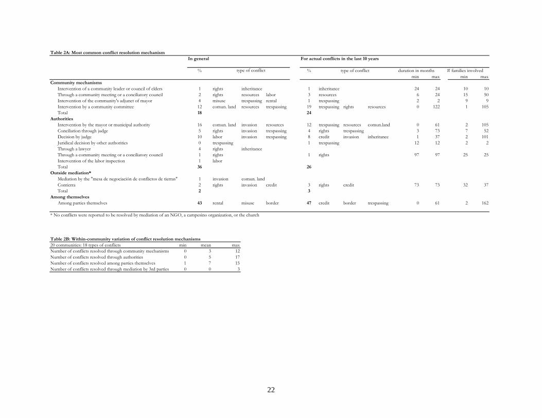
Background Information on Conflicts There is an enormous variety of both conflicts and conflict resolution mechanisms in the rural

communities studied (Table 2A). First of all, often the parties involved in a conflict will attempt

to resolve the conflict by themselves. When outside help is sought, it is most often the

(municipal) mayor, a community committee, or a judge. Sometimes the parties also resort to the

mayor’s liaison in the community, to lawyers, or even to specialized state institutions (such as

Contierra or the Instituto Nacional de Transformación Agraria). Interestingly, there appears no

clear pattern of certain institutions specializing in certain types of conflicts. For example, land

right conflicts can be resolved by village elders, a community meeting, a judge, a lawyer or state

institutions. Moreover, each of the conflict resolution mechanisms appears to be relied on for

conflicts of different severities, both in terms of duration of the conflict and in terms of the

number of parties involved.

When looking at the community level, however, we note that most communities tend to

disproportionally rely on certain types of conflict resolution mechanism, but the type of

mechanisms vary widely across communities. For example when considering 18 different types

of conflicts, 17 out of 18 types of conflicts are typically resolved through outside authorities in

one community, while in another community 12 are resolved through community mechanisms,

and in a third 15 are resolved among the parties themselves (see Table 2B). The reasons for

these differences are undoubtedly complex and may be related to the age and the history of the

community, previous conflicts, ethnic divisions, leader personalities, etc. This paper does not

aim to explain this heterogeneity. In fact, in the estimations we will control for all community

fixed effects and instead focus on how the prevalence of certain types of conflict resolution

mechanisms relates to the impact of titles on land use and credit access.

4. Identification As discussed, most variation in land titling resulted from historical decisions at the end of the

nineteenth century. While no systematic titling efforts have occurred in the regions of study since

then, individual owners might have obtained titles, e.g., through the Ley de Titulación Supletoria.

In fact, about five percent of all plots in the dataset obtained a formal title after the plot was

transferred to the current owner (and on average current owners obtained their plot 17 years ago).

Formal titles are those included in the public registry. Given that the decision to apply for such a

10

formal title is possibly not exogenous to other decisions related to the plot, we cannot use the

current title status of the plot as an independent variable. In addition, a plot’s title status might

be endogenous because certain types of households might self-select into being owners of titled

plots through the land sales market. In the sample under study, about 40 percent of all plots was

obtained through sales, while most of the other plots were obtained through inheritance. We

therefore rely on an instrumental variable estimation.

Our instruments rely on the fact that applications for titling at the end of the nineteenth

century were made simultaneously for large tracts of land, either by individuals or by community

leaders. While much of this land was subsequently fragmentized among many owners, the title

status of the different plots is still correlated. Information was collected about the geographical

location of the plots by obtaining plot-level community maps. Large estates bordering the

community, which are often not considered to be part of the community, were also included.

This allows calculating the average title status of the neighboring plots, excluding plots from the

same owner, to obtain a prediction of the title status of the plot. We will use the predicted status

of the nearest neighbor and the average title status of up to 5 neighboring plots as the instrument

for formal title in the regressions.10 The first-stage regression in Table 3 shows that these two

variables are indeed very good predictors of a plot’s title status. This holds with and without

control variables.

The validity of the instrument further depends on the plausibility of the exclusion

restriction. It seems reasonable to assume that title status of neighboring plots is uncorrelated

with many other plot and landlord characteristics, since these relate to plots of other landlords.

Yet it is not impossible that neighboring plots share certain characteristics that are both more

likely to affect their outcome today, and were important in determining their historical title

status. In particular, as discussed, land with high land quality was historically more likely to be

titled.

We hence control for plot characteristics that might be spatially correlated, and could

affect the validity of the instrument. In particular, we include dummy variables for the quality of

the plots, which was measured on a five-point scale. We also include a dummy indicating

10 For each plot, the five nearest plots were identified. If more than five plots bordered the plot, the five plots that shared the largest border were selected. If a plot had fewer than five plots with common borders, additional neighboring plots were selected based on closest distance. If among these five plots there were plots from the same owners, they were excluded, and the average title status of the remaining neighboring plots was selected.

11

whether the plot has irrigation potential (i.e., was located close to an irrigation water source, was

sufficiently flat, etc.). We further control for distance to the owner’s house and plot size, and we

allow for non-linear effects. The community-fixed effects control for all community-specific

characteristics.

In addition to plot-level geographical characteristics, we control for a number of

household level variables. Owners of neighboring plots might share certain characteristics that

not only affect their outcomes, but also relate to whether their plots have titles. This is true in

particular because owners of neighboring plots are often family members, or otherwise might

have similar characteristics that would affect the validity of the instrument. We therefore control

for ethnicity, land ownership, age, gender, literacy and Spanish-language knowledge of the

household head, household size, and machinery ownership. We also control for the number of

other households that are family in the community, whether the owner lives permanently in the

community, and whether the father of the owner lived in the community, which are all variables

that are likely to control for possible correlations between the characteristics of owners of

neighboring plots, because of past inheritance and other factors. Finally, all standard errors are

corrected for clustering at the household level to control for correlation among plots from the

same owner.

Given that some of the household variables indicated are possibly endogenous, we will

estimate all regressions both with a more limited (exogenous) set of household variables and

with the full set of household variables.11 We will additionally discuss the robustness of our

finding to inclusion or exclusion of the different plot and household control variables, which

helps sheds light on the plausibility of the exclusion restriction.12 More formally, we use over-

identification tests to further motivate the assumption.

In addition, we also estimate the model with the subset of plots that people obtained

through inheritance. If the results are driven by selection of certain types of households on titled

plots, and the instrument does not correct for this, these estimates are likely to differ substantially

11 In particular, the limited set of control variables excludes land and machinery ownership, household size, gender of the household head, whether the owner lives in the community, and whether he holds a leadership role in the community. 12 Unfortunately, there is not enough variation in the dataset to use household fixed effects to further control for possible unobservables. Some 71 percent of the households have only one plot, and of the remaining households for which we have sufficient information on the neighboring plots, only 20 households have plots both with and without title.

12

from the full sample. Inheritance itself, in this setting, does not favor certain types, as all siblings

have equal rights to the land and assets of the parents.

Another possible concern with the validity of the instruments could be that the

instruments are picking up geographical boundary effects that directly affect a plot. For example,

if actions on a neighbor’s plot are affecting the outcomes of a plot, and if those actions

themselves are correlated with the title on the neighbor’s plot, the exclusion restriction would be

violated. We can, however, try to test for a number of such possible effects. In particular, it

could be that the intensity of cultivation, and in particular the use of fertilizer and pesticides, has

spillover effects on neighboring plots. While we do not have an indicator of fertilizer or pesticide

use itself, we do have information about the intensity of the use of the neighboring plots: i.e., we

know whether the neighboring plots have horticulture products, which require a large amount of

fertilizer, and whether the owner employs day laborers on those plots, another potential indicator

of input use. We will therefore show results in which we control for these characteristics of the

neighboring plots.13

A similar concern relates to possible spillover effects of credit access. Given the

monitoring costs of the credit agencies, one could hypothesize that access to credit of

neighboring plots could be correlated, if credit agents are more likely to grant credit to a number

of neighbors that apply together, because of transaction costs and/or economies of scale. Or even

if not simultaneously, it is possible that a neighbor’s access to credit affects one’s own access, if

it implies that the credit agents already are coming to the communities for monitoring (Zegarra

and Escobal, 2007). This would be a concern for the identification strategy, as it could suggest an

alternative mechanism through which a neighbor’s title could be related to one’s credit access.

We will therefore test for robustness and control for the credit access of the owners of the

neighboring plots

Finally, it is important to point out that the identification strategy in this paper is unlikely

to hold in many other settings. In many places, recent titling programs have targeted entire

communities, and there is therefore little or no inter-community variation to exploit. In other

settings, such as in areas where the agricultural frontier has only recently closed, present titles

13 Another possible spillover effect would be related to possible infrastructure (road) investments by owners of neighboring plots that have a title. Yet, in this context, where almost all the owners are mini-fundistas, such investments by individual owners are unlikely.

13

more directly reflect efforts by current owners, and there geographical correlation is likely to be

limited.

5. The Average Impact of Titles The first four columns in Table 4 first show the results of a linear probability model for

comparison purposes. As indicated before, the efficiency of plot use is positively correlated with

the plot’s title status, yet the significance of the relationship fluctuates when different control

variables are included. We also note that the control variables are picking up a great deal of

variation in the data, and much of this variation is explained by the community fixed effects. The

R2 increases from 0.01 to 0.36. And plot and household characteristics further increase the R2 to

0.44. We find in particular that geographical characteristics (plot quality and distance), as well as

household’s human capital endowment, are related to plot use, as expected.

Column 5 to 11 then presents the IV results, including the diagnostics on the potential

weakness and the validity of the instruments (see Baum, Schaffer and Stillman, 2006). We can

reject the null in the Anderson canonical correlations test at all levels of significance indicating

that the model is identified. More importantly, the first-stage F-values, corrected for clustering at

the household level, are between 14 and 19, indicating that we do not have a weak instrument

problem. Furthermore, we cannot reject the null in the over-identification tests, indicating that

the excluded instruments are correctly excluded (P-values between 0.46 and 0.88).

Focusing on the IV results themselves, we note that while the coefficient estimates are

positive, we do not find a significant relationship between the efficiency of plot use and the

plot’s title status, and this result is robust across the different specifications. Hence, after

accounting for the endogeneity of titles, we cannot reject that, on average, titles do not have an

effect on the efficiency of plot use.

Table 5 shows the results of similar specifications for whether the plot was used only

extensively. Here we do find a negative relationship between title and plot use in both the linear

probability model and the IV. As expected, the plot-control variables are picking up much of the

variation in plot use. P-values of the over-identification test are again high (between 0.72 to 0.96)

The IV results are not significant after controlling only for plot characteristics, but becomes

significant and robust after including household-level control variables. The coefficient estimates

also become larger as we include more control variables. The coefficient estimates suggest that

14

plots with a formal title are on average 30-40 percentage points less likely to be used extensively

than other plots.

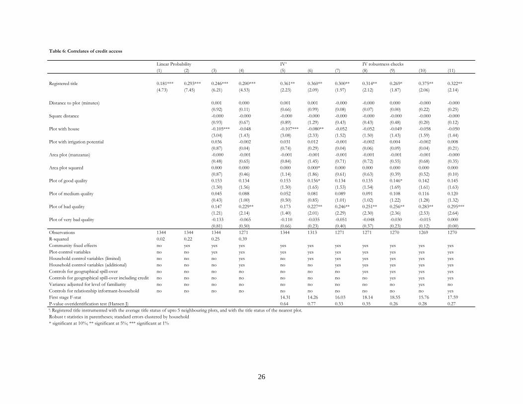
Considering then the relationship between title and access to credit, we find a strong,

significant and robust relationship. Households with titled plots are 30-40 percentage points

more likely to have access to credit (Table 6). This is a striking finding given the lack of

evidence on the effects on credit access in many other studies. One might wonder whether this is

related to the reporting by the informant. In particular, it could be the case that informants have

internalized the rules about credit access in their region and used that information in providing

answers regarding specific households. It is important to point out, however, that even if that

supposition is true, it might mainly capture a more conceptual difference between our variable of

credit access, which aims at capturing potential credit supply, and variables used in the literature.

Many other papers have looked at whether households with titles actually obtained access to

credit, and hence capture both demand and supply effects. However, households’ demand for

credit might be constraint for a number of reasons, such as high transaction costs, high interest

rates, and risk aversion (see, for example, Boucher, Barham and Carter, 2007). As such, it may

not be surprising that we find a stronger impact of titles, when only the impact on credit supply is

considered. Another potential difference is that distance to credit institutions might be lower in

the regions studied than in some of the other rural settings that have been analyzed in other

studies. In particular, local branches of private banks and/or credit agencies, are relatively

widespread, and households are also actually taking out loans from such institutions. On average

10 households per community (the median is 6) have credit from a financial institution that

demands land as collateral. This is often related to intensive horticulture production, and

therefore suggests an important difference with studies in urban settings. In the context of urban

squatting communities, households are often shown to invest in home improvements. In the rural

setting we study however, households invest in more direct productive purposes, which could

contribute to the higher credit supply response.

Finally, we also estimated the model using the household’s living standard as an outcome

variable. For this variable, we reject the over-identification test for the IV estimation exclusion,

indicating that the exclusion restriction is not valid for this particular outcome variable. While

including plot and household characteristics does decrease the Hansen J-statistic (as we would

expect), it is 2.75 in the estimation with all household control variables included, which implies

15

that we reject the null-hypothesis at the 10 percent level. This implies that our identification

strategy does not allow us to identify the overall effect of title on household welfare. This may

partly be explained by the fact that household welfare is affected by many more factors than

either plot use or credit access, some of which might be correlated among neighbors.

Robustness Checks The estimates on the subset of plots that were obtained through inheritance are largely similar to

the results for the full sample.14 Interestingly, the point estimates of the relationship between

titles and extensive use and credit, are in fact higher in the IV than the estimates of the full

sample, but the results are not significant at the 10 percent level. The later can be explained, in

part, by the smaller sample sizes.

Column 8 in Tables 4-6 shows the results of the estimations that control for possible

geographical spillover effects that might affect the validity of the instrument. In particular, we

include as extra control variables whether the five neighboring plots (used for the IV) were used

for horticulture products (which tend to be correlated with high use of fertilizer and pesticides)

and whether day laborers were used on those plots (another indicator of high input use). We

include variables indicating whether at least one of the neighboring plots had horticulture

products or day laborers, as well as variables indicating the average outcomes of the five plots

for these indicators. Column 8 of each table shows that the results are remarkably robust for

inclusion of control variables to capture possible geographical spillover effects. In column 9, we

additionally include a variable indicating whether at least one of the households with a

neighboring plot has access to credit, as well as variables indicating the average credit outcomes

of the households owning the five neighboring plots. The results are robust, suggesting that they

are not driven by possible scale-economies/transaction costs in credit access. Overall, these

results further support the use of the instruments.

Finally columns 10 and 11 present robustness checks related to the use of the key

informant. In particular, column 10 shows an estimation that corrects the variances for the level

of familiarity that the informant had with each household.15 For each household, informants were

asked how well they knew the household and the situation of the household’s plots. This allows

14 Estimates available from author

16

estimating a weighted 2SLS that accounts for the fact that the noise is likely to be larger for those

households for which informants report having less good information. Alternatively, in column

11, we include an estimation that specifically adds a number of controls capturing the

relationship between the informant and each household: in addition to the familiarity variable, it

also includes a dummy variable to indicate whether they are from the same ethnicity, and another

dummy variable to indicate whether they have the same living standard. All results are robust in

both these alternative models, and are in fact sometimes more significant. This suggests that the

use of the key informant itself is not driving the results in this paper.

6. Does the Impact of Titles Depend on Conflicts and Conflict Resolution Mechanisms? Overall, the IV results present mixed evidence on the average impact of titles, suggesting titling

facilitates access to credit and affects plot use in some dimensions, but not others. The impact of

titles is generally believed to come from an increase in property rights security. We now analyze

whether, in the sample studied, property rights conflicts on plots are indeed less likely on plots

with a formal title. Table 7 shows the linear probability and the IV results indicating the

relationship between titles and the present or past occurrence of a land rights conflict on a plot.16

The IV shows a strong and robust relationship, suggesting that property rights conflicts are more

than 20 percentage points less likely on plots with a formal title.

Given the direct relationship between titles and plot-level conflicts, it seems important to

consider whether the impact of titles might vary depending on the conflict situation in a

community. In particular, given that titles seem to reduce the likelihood of a conflict on a plot,

one would expect the value of title to increase the more severe the conflict situation is in a

particular community. In other words, we hypothesize that the effects of titles on plot use is

larger in communities where conflicts take a long time to be resolved, or in communities with

recent land rights conflicts. Moreover, we also analyze whether the relationship between titles

and plot use depends on the conflict resolution mechanisms that are used in a community.

15 The level of familiarity can vary across informants and households because of community size, experience of the leader, differences in ethnic composition, differences in immigration in the different communities, etc. 16 This excludes border conflicts with neighboring plots, as the identification strategy is clearly not appropriate for such conflicts.

17

By including interaction effects of the (instrumented) title with variables capturing the

prevalence of different type of conflicts and conflict resolution mechanisms, we shed light on

how the effects of title differ with these variables. For the first-stage estimation, the two

instruments for title were interacted with these same community-conflict variables. The first-

stage F-values for title and for the interaction effects of title are lower than before but still

relatively high (F-value between 8.5 and 11)

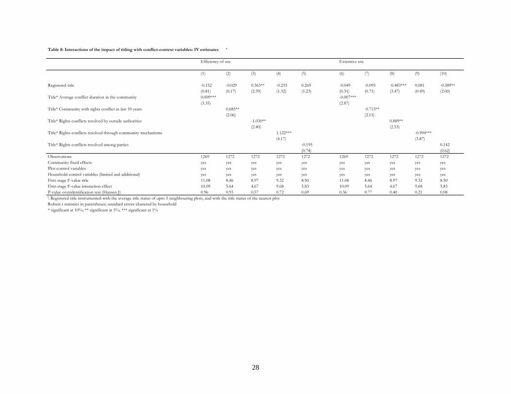
Table 8 shows that titles do have an effect on the efficiency of plot use once community

conflicts are taken into account.17 In particular, the longer the average duration of conflicts, the

stronger the positive effect of titles on the efficiency of plot use, and the stronger the negative

relationship between titles and extensive use. We also find some evidence that the positive

effects of title are stronger in communities that had a property rights conflict in the last 10 years.

In other words, in communities where conflicts tend to be resolved relatively quickly, and in

communities without recent land rights conflicts, a formal title status seems to be much less

important for efficient plot use. On the other hand, the effect of titles on access to credit does not

appear to depend on the conflict or conflict resolution mechanisms, possibly because information

on community-level conflicts is not necessarily available to lending institutions. While arguably

not surprising, the plot use results potentially indicate a lesson for targeting of titling efforts. It

also may indicate the importance of alternative property right enforcement mechanisms as

substitutes for formal titling.

The results in column 3 to 5, and 8 to 10, shed some further, somewhat intriguing, light

on this issue. We find that titles have a positive effect on efficiency in communities where

property rights conflicts are typically resolved through community mechanisms, but a negative

effect in communities where rights conflicts are typically resolved by outside authorities. When

using information about actual resolution mechanisms used for property rights conflicts in the

last 10 years, we similarly find a positive effect of titles on efficiency in communities where

property rights conflicts were resolved through community mechanisms, but a negative, though

insignificant, effect in communities where rights conflicts were resolved by outside authorities.

One possible interpretation of this finding is that, in the context of rural Guatemala,

informal community mechanisms seem to complement, rather than substitute for, the effect of a

formal title, presumably because they typically help enforce the property right in case the owner

17 Results are robust to inclusion of only the limited or the full set of household control variables.

18

has a formal title. Outside authorities may not play a similar role. Yet, there clearly are many

possible confounding factors that make the interpretation of this finding difficult. The use of a

particular of conflict resolution mechanism in a community is not exogenous and is likely to

reflect the possibly long history of conflicts in those communities.18 This dataset does not allow

analyzing the causal factors in more detail, given that there are only 20 communities. Including

further interaction effects to control for possible confounding factors is limited for the same

reason, aside from leading to weak instruments problems.

Nevertheless, the findings do suggest that the impacts of formal titles on plot use vary

considerably with the conflict situation in a community, and that, even within small geographical

areas there might be quite a large heterogeneity. They also suggest that the relationship between

the impacts of titles and existing conflict resolution mechanisms can be complex.

7. Conclusions This paper has analyzed the effect of titles on plot use and credit access and investigated whether

the effects of titles vary with the history of conflict and existing conflict resolution mechanisms

in the community. Overall, we find that the effects of titles on the efficiency of plot use depend

on the conflict context of the community. This is not necessarily surprising, as a title’s value and

effects are likely to depend on whether a formal title helps to secure property rights, and on

whether there are alternative mechanisms that might secure such rights. While it is hard to

specifically identify which aspects of the conflict context might matter the most, the results

indicate some intriguing patterns, and clearly suggest that community context is key to

understanding the potential value of a registered title. Moreover, this context might matter more

for some outcomes (efficiency) than for others (credit).

Overall, the results suggest that there is a great deal of room for future research that

attempts to understand the relationship between titles and conflict in Latin America. It also

indicates that the design and targeting of titling policies can benefit from carefully accounting for

the existing conflict situation and the conflict resolution mechanisms, as they are likely to affect

the pay-offs and trade-offs of such interventions.

18 It should be noted, however, that in this dataset, the duration of the conflict does not appear to be correlated with the conflict resolution mechanism. See also the descriptive analysis in Table 2.

19

References Acemoglu, D., and S. Johnson, 2005. “Unbundling Institutions.” Journal of Political Economy

(113): 949-995.

Acemoglu, D., S. Johnson and J. Robinson. 2001. “The Colonial Origins of Comparative

Development: An Empirical Investigation.” American Economic Review 91: 1369-1401.

Baum, C.F., M.E. Schaffer and S. Stillman. 2006. “Ivreg2: Stata Module for Extended

Instrumental Variables/2SLS, GMM and AC/HAC, LIML and K-class Regression.”

http://ideas.repec.org/c/boc/bocode/s425401.html

Besley, T. 1995. “Property Rights and Investment Incentives: Theory and Evidence from

Ghana.” Journal of Political Economy 103(5): 903-37.

Boucher, S., B. Barham and M. Carter. 2005. “The Impact of Market-Friendly Reforms on

Credit and Land Markets in Honduras and Nicaragua.” World Development 33(1): 107-

128.

----. 2007. “When Land Titles Are NOT the Constraint: Complementary Financial Policies to

Enhance Agricultural Productivity.” Davis and Madison, United States: University of

California Davis and University of Wisconsin-Madison. Mimeographed document.

Braselle, A-S., F. Gaspart and J-P. Platteau. 2002. “Land Tenure Security and Investment

Incentives: Puzzling Evidence from Burkina Faso.” Journal of Development Economics

67(2): 373-418.

Carter, M., and P. Olinto. 2003. “Getting Institutions ‘Right’ for Whom? Credit Constraints and

the Impact of Property Rights on the Quantity and Composition of Investment.”

American Journal of Agricultural Economics 85(1): 173-186.

Chang, C.R. 2002. “Legal Restrictions to Land Rental Markets in Guatemala.” Background

report prepared for FAORLC workshop on land rental markets in Latin America,

Santiago, Chile, August 1-2.

Di Tella, R., S. Galiani and E. Schargrodsky. 2007. “The Formation of Beliefs: Evidence from

the Allocation of Land Titles to Squatters.” Quarterly Journal of Economics 122(1): 209-

241.

Field, E. 2005. “Property Rights and Investment in Urban Slums.” Journal of the European

Economic Association 3(2-3): 279-290.

20

Galiani, S., and E. Schargrodsky. 2007. “Property Rights for the Poor: Effects of Land Titling.”

Buenos Aires, Argentina: Universidad Torcuato di Tella. Mimeographed document.

Grandin, G. 2000. The Blood of Guatemala: A History of Race and Nation. Durham, United

States and London, United Kingdom: Duke University Press.

Lanjouw, J., and P. Levy. 2002. “Untitled: A Study of Formal and Informal Property Rights in

Urban Ecuador.” Economic Journal 112(482): 986-1019.

Macours, K. 2003. “Comparing a Direct with an Indirect Approach to Collecting Household

Level Data: Who Tells the Truth about What?” Washington, DC, United States: Johns

Hopkins University. Mimeographed document.

----. 2007. “Ethnic Divisions, Contract Choice and Search Costs in the Guatemalan Land Rental

Market.” Washington, DC, United States: Johns Hopkins University. Mimeographed

document.

Macours, K., A. de Janvry and E. Sadoulet. 2007. “Insecurity of Property Rights and Matching in

the Tenancy Market.” Washington, DC, United States: Johns Hopkins University.

Mimeographed document.

McCreery, D. 1994. “State Power, Indigenous Communities, and Land in Nineteenth-Century

Guatemala, 1820-1920.” In: C.A. Smith, editor. Guatemalan Indians and the State: 1540-

1988. Austin, United States: University of Texas Press.

Naylor, R.A. 1967. “Guatemala: Indian Attitudes towards Land Tenure.” Journal of Inter-

American Studies 9(4): 619-639.

Takasaki, Y., B. Barham and O.T. Coomes. 2000. “Rapid Rural Appraisal in Humid Tropical

Forests: An Asset Possession-based Approach and Validation Methods for Wealth

Assessment among Forest Peasant Households.” World Development 28(11): 1161-77.

Zegarra, E., and J. Escobal. 2007. “Titling, Credit Constraints and Rental Markets in Rural Peru:

Exploring Channels and Conditioned Impacts.” Lima Peru: Grupo de Análisis para el

Desarrollo (GRADE). Mimeographed document.

21

Table 1A: Characteristics informants and average landowning households

Informant Landowninghousehold

20 1120Individual characteristics

Age household head (years) 46 44Literate household head (%) 75 64Speaks Spanish (%) 95 92Male household head (%) 95 86Has always lived in the community (%) 100 82Father originally from the community (%) 60 51

Household characteristicsLand owned (cuerdas) 43 176Owns agricultural tools (%) 75 54Household size (number) 4.45 3Number of related families in community 3.85 2.58Ethnicity Ladino (%) 15 20 Mam (%) 40 36 Qeqchi (%) 0 7 Poqom (%) 40 31 Achi (%) 5 4Livingstandard Good livingstandard (%) 10 25 Regular livingstandard (%) 80 56 Low livingstandard(%) 10 19

Table 1B: Descriptive statistics of outcome variablesNo title Title Significance

1440 402 differencea

Plot-level outcomesEfficient use (used at full potential) 0.74 0.86 ***Extensive use (pasture, forest, idle) 0.13 0.09 **

Household-level outcomesAccess to credit 0.65 0.87 ***Good living standard 0.22 0.55 ***

a: standard errors corrected for clustering at household level

22

Table 2A: Most common conflict resolution mechanismIn general For actual conflicts in the last 10 years

% %min max min max

Community mechanismsIntervention of a community leader or council of elders 1 rights inheritance 1 inheritance 24 24 10 10Through a community meeting or a conciliatory council 2 rights resources labor 3 resources 6 24 15 50Intervention of the community's adjunct of mayor 4 misuse trespassing rental 1 trespassing 2 2 9 9Intervention by a community committee 12 comun. land resources trespassing 19 trespassing rights resources 0 122 1 105Total 18 24

AuthoritiesIntervention by the mayor or municipal authority 16 comun. land invasion resources 12 trespassing resources comun.land 0 61 2 105Conciliation through judge 5 rights invasion trespassing 4 rights trespassing 3 73 7 52Decision by judge 10 labor invasion trespassing 8 credit invasion inheritance 1 37 2 101Juridical decision by other authorities 0 trespassing 1 trespassing 12 12 2 2Through a lawyer 4 rights inheritanceThrough a community meeting or a conciliatory council 1 rights 1 rights 97 97 25 25Intervention of the labor inspection 1 laborTotal 36 26

Outside mediation*Mediation by the "mesa de negociación de conflictos de tierras" 1 invasion comun. landContierra 2 rights invasion credit 3 rights credit 73 73 32 37Total 2 3

Among themselvesAmong parties themselves 43 rental misuse border 47 credit border trespassing 0 61 2 162

* No conflicts were reported to be resolved by mediation of an NGO, a campesino organization, or the church

Table 2B: Within-community variation of conflict resolution mechanisms20 communities: 18 types of conflicts min mean maxNumber of conflicts resolved through community mechanisms 0 3 12Number of conflicts resolved through authorities 0 5 17Number of conflicts resolved among parties themselves 1 7 15Number of conflicts resolved through mediation by 3rd parties 0 0 3

# families involvedtype of conflict type of conflict duration in months

23

Table 3: First stage regression of title status plot

(1) (2) (3)

Average title status 5 closest neighboring plots 0.501*** 0.186** 0.222***(7.17) (2.52) (3.32)

Title status nearest plot 0.206*** 0.133*** 0.098**(3.66) (2.93) (2.23)

Constant 0.051** -0.019 0.170(2.29) (0.17) (0.81)

Plot-control variables no yes yesHousehold-control variables no no yes

Observations 1348 1348 1272R-squared 0.38 0.56 0.65Standard errors corrected for clustering at household level* significant at 10%; ** significant at 5%; *** significant at 1%

24

Table 4: Correlates of the efficiency of plot use

Linear Probability IVa IV robustness checks(1) (2) (3) (4) (5) (6) (7) (8) (9) (10) (11)

Registered title 0.119*** 0.091 0.110** 0.087** 0.271 0.276 0.169 0.162 0.155 0.223 0.187(3.00) (1.52) (2.22) (2.07) (1.64) (1.56) (1.10) (1.15) (1.11) (1.21) (1.28)

Distance to plot (minutes) -0.003* -0.004** -0.003** -0.004** -0.004** -0.004** -0.004** -0.004** -0.004***(1.94) (2.43) (2.29) (2.50) (2.58) (2.50) (2.45) (2.39) (2.60)

Square distance 0.000 0.000* 0.000 0.000* 0.000** 0.000* 0.000* 0.000* 0.000**(1.39) (1.82) (1.54) (1.94) (1.98) (1.92) (1.87) (1.92) (2.04)

Plot with house -0.042 -0.054 -0.044 -0.057 -0.057 -0.055 -0.054 -0.061 -0.054(1.23) (1.55) (1.29) (1.63) (1.62) (1.57) (1.53) (1.64) (1.54)

Plot with irrigation potential -0.047 -0.032 -0.054 -0.081 -0.032 -0.034 -0.032 -0.036 -0.030(0.89) (0.75) (0.95) (1.50) (0.74) (0.78) (0.75) (0.82) (0.69)

Area plot (manzanas) -0.001 -0.004 -0.001 -0.001 -0.004 -0.004 -0.004 -0.005* -0.004(0.28) (1.10) (0.60) (0.45) (1.19) (1.17) (1.13) (1.78) (1.15)

Area plot squared 0.000 0.000 0.000 0.000 0.000 0.000 0.000 0.000 0.000(0.35) (0.81) (0.62) (0.32) (0.91) (0.89) (0.86) (1.54) (0.84)

Plot of good quality 0.091 0.061 0.091 0.070 0.061 0.066 0.067 0.067 0.065(1.12) (0.75) (1.11) (0.85) (0.74) (0.80) (0.81) (0.82) (0.80)

Plot of medium quality 0.026 -0.003 0.036 0.020 -0.002 0.003 0.004 0.018 0.009(0.32) (0.04) (0.43) (0.25) (0.03) (0.04) (0.05) (0.21) (0.10)

Plot of bad quality -0.060 -0.073 -0.024 -0.017 -0.058 -0.052 -0.050 -0.032 -0.035(0.57) (0.68) (0.22) (0.16) (0.54) (0.49) (0.47) (0.30) (0.33)

Plot of very bad quality -0.272** -0.219 -0.239* -0.190 -0.208 -0.200 -0.195 -0.174 -0.181(2.02) (1.53) (1.76) (1.37) (1.46) (1.39) (1.36) (1.22) (1.26)

Observations 1348 1348 1348 1272 1348 1314 1272 1272 1271 1270 1271R-squared 0.01 0.36 0.38 0.44Community fixed effects no yes yes yes yes yes yes yes yes yes yesPlot-control variables no no yes yes yes yes yes yes yes yes yesHousehold control variables (limited) no no no yes no yes yes yes yes yes yesHousehold control variables (additional) no no no yes no no yes yes yes yes yesControls for geographical spill-over no no no no no no no yes yes yes yesControls for geographical spill-over including credit no no no no no no no no yes yes yesVariance adjusted for level of familiarity no no no no no no no no no yes noControls for relationship informant-household no no no no no no no no no no yesFirst stage F-stat 14.40 14.29 16.05 18.15 18.57 15.77 17.60P-value overidentification test (Hansen J) 0.68 0.66 0.88 0.83 0.88 0.46 0.82

a: Registered title instrumented with the average title status of upto 5 neighbouring plots, and with the title status of the nearest plot.Robust t statistics in parentheses; standard errors clustered by household* significant at 10%; ** significant at 5%; *** significant at 1%

25

Table 5: Correlates of the extensive of plot use (plot used for pasture, forest, or idle)

Linear Probability IVa IV robustness checks(1) (2) (3) (4) (5) (6) (7) (8) (9) (10) (11)

Registered title -0.031 -0.030 -0.078** -0.093*** -0.201 -0.268* -0.302** -0.347*** -0.352*** -0.451*** -0.362***(1.32) (0.71) (1.97) (3.04) (1.55) (1.92) (2.22) (2.69) (2.72) (2.66) (2.71)

Distance to plot (minutes) 0.003** 0.005*** 0.004** 0.004*** 0.005*** 0.005*** 0.005*** 0.005*** 0.005***(2.40) (2.86) (2.57) (2.90) (3.07) (3.13) (3.13) (2.78) (3.15)

Square distance -0.000** -0.000** -0.000** -0.000*** -0.000*** -0.000*** -0.000*** -0.000** -0.000***(2.21) (2.42) (2.34) (3.01) (2.66) (2.73) (2.72) (2.41) (2.75)

Plot with house -0.088*** -0.082*** -0.086*** -0.075** -0.073** -0.073** -0.073** -0.050 -0.074**(3.13) (2.73) (3.01) (2.51) (2.34) (2.34) (2.32) (1.56) (2.35)

Plot with irrigation potential -0.048 -0.054* -0.043 -0.042 -0.055* -0.053 -0.052 -0.061* -0.053(1.47) (1.71) (1.25) (1.26) (1.68) (1.58) (1.55) (1.80) (1.59)

Area plot (manzanas) 0.006*** 0.008*** 0.006*** 0.005*** 0.008*** 0.008*** 0.008*** 0.007*** 0.008***(3.22) (3.88) (3.22) (2.88) (3.77) (3.69) (3.67) (3.12) (3.50)

Area plot squared -0.000** -0.000*** -0.000** -0.000** -0.000*** -0.000*** -0.000*** -0.000** -0.000***(2.32) (2.98) (2.32) (2.18) (2.90) (2.87) (2.85) (2.47) (2.70)

Plot of good quality -0.136 -0.084 -0.136 -0.117 -0.083 -0.079 -0.078 -0.089 -0.074(1.60) (1.08) (1.60) (1.51) (1.07) (0.98) (0.96) (1.10) (0.92)

Plot of medium quality -0.088 -0.044 -0.095 -0.073 -0.046 -0.043 -0.041 -0.057 -0.038(1.03) (0.56) (1.11) (0.94) (0.59) (0.52) (0.50) (0.69) (0.47)

Plot of bad quality 0.126 0.176* 0.098 0.094 0.138 0.135 0.136 0.109 0.129(1.21) (1.77) (0.93) (0.96) (1.39) (1.34) (1.35) (1.08) (1.28)

Plot of very bad quality 0.322** 0.316** 0.297** 0.255* 0.288** 0.283* 0.285* 0.260* 0.281*(2.33) (2.17) (2.13) (1.83) (2.00) (1.93) (1.95) (1.78) (1.92)

Observations 1348 1348 1348 1272 1348 1314 1272 1272 1271 1270 1271R-squared 0.00 0.08 0.21 0.24Community fixed effects no yes yes yes yes yes yes yes yes yes yesPlot-control variables no no yes yes yes yes yes yes yes yes yesHousehold control variables (limited) no no no yes no yes yes yes yes yes yesHousehold control variables (additional) no no no yes no no yes yes yes yes yesControls for geographical spill-over no no no no no no no yes yes yes yesControls for geographical spill-over including credit no no no no no no no no yes yes yesVariance adjusted for level of familiarity no no no no no no no no no yes noControls for relationship informant-household no no no no no no no no no no yesFirst stage F-stat 14.40 14.29 16.05 18.15 18.57 15.77 17.60P-value overidentification test (Hansen J) 0.96 0.83 0.93 0.83 0.95 0.72 0.94

a: Registered title instrumented with the average title status of upto 5 neighbouring plots, and with the title status of the nearest plot.Robust t statistics in parentheses; standard errors clustered by household* significant at 10%; ** significant at 5%; *** significant at 1%

26

Table 6: Correlates of credit access

Linear Probability IVa IV robustness checks(1) (2) (3) (4) (5) (6) (7) (8) (9) (10) (11)

Registered title 0.181*** 0.293*** 0.246*** 0.200*** 0.361** 0.360** 0.300** 0.314** 0.269* 0.375** 0.322**(4.73) (7.45) (6.21) (4.53) (2.23) (2.09) (1.97) (2.12) (1.87) (2.06) (2.14)

Distance to plot (minutes) 0.001 0.000 0.001 0.001 -0.000 -0.000 0.000 -0.000 -0.000(0.92) (0.11) (0.66) (0.99) (0.08) (0.07) (0.00) (0.22) (0.25)

Square distance -0.000 -0.000 -0.000 -0.000 -0.000 -0.000 -0.000 -0.000 -0.000(0.93) (0.67) (0.89) (1.29) (0.43) (0.43) (0.48) (0.20) (0.12)

Plot with house -0.105*** -0.048 -0.107*** -0.080** -0.052 -0.052 -0.049 -0.058 -0.050(3.04) (1.43) (3.08) (2.33) (1.52) (1.50) (1.43) (1.59) (1.44)

Plot with irrigation potential 0.036 -0.002 0.031 0.012 -0.001 -0.002 0.004 -0.002 0.008(0.87) (0.04) (0.74) (0.29) (0.04) (0.06) (0.09) (0.04) (0.21)

Area plot (manzanas) -0.000 -0.001 -0.001 -0.001 -0.001 -0.001 -0.001 -0.001 -0.000(0.48) (0.65) (0.84) (1.45) (0.71) (0.72) (0.55) (0.68) (0.35)

Area plot squared 0.000 0.000 0.000 0.000* 0.000 0.000 0.000 0.000 0.000(0.87) (0.46) (1.14) (1.86) (0.61) (0.63) (0.39) (0.52) (0.10)

Plot of good quality 0.153 0.134 0.153 0.156* 0.134 0.135 0.146* 0.142 0.145(1.50) (1.56) (1.50) (1.65) (1.53) (1.54) (1.69) (1.61) (1.63)

Plot of medium quality 0.045 0.088 0.052 0.081 0.089 0.091 0.108 0.116 0.120(0.43) (1.00) (0.50) (0.85) (1.01) (1.02) (1.22) (1.28) (1.32)

Plot of bad quality 0.147 0.229** 0.173 0.227** 0.246** 0.251** 0.256** 0.283** 0.295***(1.21) (2.14) (1.40) (2.01) (2.29) (2.30) (2.36) (2.53) (2.64)

Plot of very bad quality -0.133 -0.065 -0.110 -0.035 -0.051 -0.048 -0.030 -0.015 0.000(0.81) (0.50) (0.66) (0.23) (0.40) (0.37) (0.23) (0.12) (0.00)

Observations 1344 1344 1344 1271 1344 1313 1271 1271 1270 1269 1270R-squared 0.02 0.22 0.25 0.39Community fixed effects no yes yes yes yes yes yes yes yes yes yesPlot-control variables no no yes yes yes yes yes yes yes yes yesHousehold control variables (limited) no no no yes no yes yes yes yes yes yesHousehold control variables (additional) no no no yes no no yes yes yes yes yesControls for geographical spill-over no no no no no no no yes yes yes yesControls for geographical spill-over including credit no no no no no no no no yes yes yesVariance adjusted for level of familiarity no no no no no no no no no yes noControls for relationship informant-household no no no no no no no no no no yesFirst stage F-stat 14.31 14.26 16.03 18.14 18.55 15.76 17.59P-value overidentification test (Hansen J) 0.64 0.77 0.33 0.35 0.26 0.28 0.27a: Registered title instrumented with the average title status of upto 5 neighbouring plots, and with the title status of the nearest plot.Robust t statistics in parentheses; standard errors clustered by household* significant at 10%; ** significant at 5%; *** significant at 1%

27

Table 7: Correlates of plot-level property right conflict

Linear Probability IVa IV robustness checks(1) (2) (3) (4) (5) (6) (7) (8) (9) (10) (11)

Registered title -0.071*** -0.064*** -0.044*** -0.063*** -0.203*** -0.219*** -0.219*** -0.223*** -0.215*** -0.280*** -0.227***(4.58) (3.97) (2.84) (3.55) (2.83) (2.92) (3.04) (3.18) (3.15) (3.07) (3.15)

Distance to plot (minutes) -0.001** -0.001*** -0.001 -0.001 -0.001** -0.001* -0.001* -0.001 -0.001*(2.45) (3.13) (1.20) (0.91) (1.98) (1.85) (1.92) (1.17) (1.67)

Square distance 0.000** 0.000*** 0.000 0.000 0.000 0.000 0.000 0.000 0.000(2.35) (2.83) (1.58) (0.85) (1.27) (1.16) (1.21) (0.40) (0.91)

Plot with house -0.045*** -0.049*** -0.043*** -0.042*** -0.043*** -0.043*** -0.043*** -0.045*** -0.044***(3.57) (3.79) (3.20) (3.00) (3.19) (3.15) (3.20) (3.00) (3.25)

Plot with irrigation potential 0.018 0.017 0.025* 0.021 0.017 0.017 0.016 0.018 0.015(1.48) (1.23) (1.71) (1.38) (1.10) (1.13) (1.06) (1.05) (0.95)

Area plot (manzanas) -0.001 -0.003 -0.000 -0.000 -0.002 -0.002 -0.002 -0.003 -0.002(0.78) (1.40) (0.15) (0.45) (1.04) (1.02) (1.04) (1.01) (1.04)

Area plot squared 0.000 0.000 0.000 0.000 0.000 0.000 0.000 0.000 0.000(0.84) (1.37) (0.26) (0.62) (0.93) (0.91) (0.95) (0.91) (0.96)

Plot of good quality -0.040 -0.049 -0.040 -0.034 -0.049 -0.051 -0.053 -0.059 -0.050(1.07) (1.30) (1.02) (0.85) (1.25) (1.29) (1.34) (1.43) (1.25)

Plot of medium quality -0.045 -0.050 -0.055 -0.046 -0.052 -0.054 -0.057 -0.070* -0.055(1.15) (1.27) (1.39) (1.14) (1.31) (1.34) (1.40) (1.68) (1.35)

Plot of bad quality 0.100* 0.104* 0.065 0.079 0.076 0.076 0.075 0.058 0.071(1.73) (1.74) (1.20) (1.42) (1.36) (1.35) (1.34) (1.00) (1.27)

Plot of very bad quality 0.152* 0.161* 0.120 0.145* 0.140* 0.137* 0.134* 0.113 0.130(1.80) (1.85) (1.54) (1.82) (1.74) (1.70) (1.65) (1.42) (1.64)

Observations 1348 1348 1348 1272 1348 1314 1272 1272 1271 1270 1271R-squared 0.09 0.95 0.95 0.95Community fixed effects no yes yes yes yes yes yes yes yes yes yesPlot-control variables no no yes yes yes yes yes yes yes yes yesHousehold control variables (limited) no no no yes no yes yes yes yes yes yesHousehold control variables (additional) no no no yes no no yes yes yes yes yesControls for geographical spill-over no no no no no no no yes yes yes yesControls for geographical spill-over including credit no no no no no no no no yes yes yesVariance adjusted for level of familiarity no no no no no no no no no yes noControls for relationship informant-household no no no no no no no no no no yesFirst stage F-stat 14.40 14.29 16.05 18.15 18.57 15.77 17.60P-value overidentification test (Hansen J) 0.21 0.29 0.48 0.48 0.53 0.52 0.49a: Registered title instrumented with the average title status of upto 5 neighbouring plots, and with the title status of the nearest plot.Robust t statistics in parentheses; standard errors clustered by household* significant at 10%; ** significant at 5%; *** significant at 1%

28

Table 8: Interactions of the impact of titling with conflict-context variables: IV estimates a

Efficiency of use Extensive use

(1) (2) (3) (4) (5) (6) (7) (8) (9) (10)

Registered title -0.152 -0.029 0.363** -0.255 0.269 -0.049 -0.095 -0.483*** 0.081 -0.389**(0.81) (0.17) (2.39) (1.32) (1.23) (0.31) (0.71) (3.47) (0.49) (2.00)

Title* Average conflict duration in the community 0.009*** -0.007***(3.35) (2.87)

Title* Community with rights conflict in last 10 years 0.685** -0.713**(2.06) (2.15)

Title* Rights conflicts resolved by outside authorities -1.030** 0.889**(2.40) (2.53)

Title* Rights conflicts resolved through community mechanisms 1.122*** -0.994***(4.17) (3.87)

Title* Rights conflicts resolved among parties -0.195 0.142(0.74) (0.62)

Observations 1269 1272 1272 1272 1272 1269 1272 1272 1272 1272Community fixed effects yes yes yes yes yes yes yes yes yes yesPlot-control variables yes yes yes yes yes yes yes yes yes yesHousehold control variables (limited and additional) yes yes yes yes yes yes yes yes yes yesFirst-stage F-value title 11.08 8.46 8.97 9.32 8.50 11.08 8.46 8.97 9.32 8.50First-stage F-value interaction effect 10.09 5.64 4.67 9.68 5.83 10.09 5.64 4.67 9.68 5.83P-value overidentification test (Hansen J) 0.96 0.93 0.57 0.72 0.69 0.36 0.77 0.40 0.21 0.08a: Registered title instrumented with the average title status of upto 5 neighbouring plots, and with the title status of the nearest plotRobust t statistics in parentheses; standard errors clustered by household* significant at 10%; ** significant at 5%; *** significant at 1%