R- 548

SENSORY, DECISION AND CONTROL SYSTEMS APRIL TO JULY 1966

by Louis L. Sutro, et al.

November 1966

i --_- .-- - I FOR OFFICIAL USE ONLY This document has been prepared for Instrumentation Laboratory use ail& f o r contralledexternaldistrlbution. 2eWoduo- t i onor fu r the rd i s seno ina t ion i sno tau tho - rized without express written approval of M.I.T. This dooummt has no t been reviewed b y t h e D l r e c t o r a t e f o r SecurityRavlew, OSD, and therefore, is not for publio release.

LABURATURY Cambridge 39, M U S .

https://ntrs.nasa.gov/search.jsp?R=19670016626 2018-12-07T04:05:07+00:00Z

c

R-548

SENSORY, DECISION AND CONTROL SYSTEMS APRIL TO JULY 1966

bY

Louis L. Sutro, et al.

November 1966

A report of work performed from April 16 to July 15, 1966 under NASA Contract NSR 22009-138, and from October 1, 1965 to

July 15, 1966 under Air Force Contract AF 04(695)-917.

INSTRUMENTATION LABORATORY MASSACHUSETTS INSTITUTE OF TECHNOLOGY

CAMBRIDGE, MASSACHUSETTS Prepared for publication by Jackson G Moreland

Division of United Engineers G Constructors, !nc.

Approved ( / A s s o c i a t e Director

Approved Deputy Di rector /

ACKNOWLEDGEMENT

Sections 1, 2, 3 and 5 and subsection 4 . 7 were prepared under the auspices of DSR Project 55-25700, sponsored by the Bioscience Division of the National Aeronautics and Space Administration through Contract NSR-22-009-138. tions 4 and 6, with the exception of subsection 4.7, were prepared under the auspices of DSR Project 52-25600, sponsored by the Space Systems Division, U . S. Air Force Systems Command through Contract A F 04(695)-917.

Sec-

Major contributions to the program have been made by consultants to the

Laboratory, by members of the Sensory, Decision and Control Systems (SDCS) Group of the Longspur Section of the Instrumentation Laboratory and other members of the Longspur Section:

Consult ants -

D r . Warren S. McCulloch Dr . William L. Kilmer Dr . Car l Sagan

The SDCS Group -

Jay Blum - Staff Member Richard Catchpole - Research Assistant .Jerome L. Krasner - Staff Member D r . Roberto Moreno-Diaz - Staff Member David Peterson - Research Assistant Louis Sutro - Assistant Director David Tweed - Staff Member

Other Members of the Longspur Section -

Joseph Convers - Staff Member

Editorial assistance w a s provided by David Lampert , a research assistant, who joined the SDCS Group after the period of this report .

ii

ABSTRACT

The quarter reported here for the NASA contract, and the longer period reported for the A i r Force contract, saw the development of two system concepts for the transmission of video data from a remote location to Earth. simpler system, a stereoscopic outline together with other data such a s reflect-

ance and possibly the texture of objects will be transmitted to Earth. The ob- jects considered a r e those larger than a predetermined s ize and within a pre- determined range. Earth he wi l l decide what objects he would like pictured in full TV frames and order these transmitted.

In the

F rom the stereoscopic outlines presented to the operator on

In the more elaborate system, TV cameras wi l l be carr ied on a vehicle and the direction in which the vehicle moves will be chosen by an onboard decision computer. Perceptual decisions may also be made to identify objects whose characterist ics have been reported to Earth and whose value to the Earth ob- se rver has been communicated back to the perceptual computer. of cameras, perceptual computer, decision computer and vehicle is called a robot.

The assembly

Photosensors for this robot a r e television cameras, the f i rs t models of wnicn have been tested under computer controi. computer and the decision computer has been simulated. It consists of 1 2 mo- dules, each of which makes an initial guess a s to what the response to incoming data should be. a nonlinear fashion with the data coming directly into it to a r r ive at a mixed guess as to what act should be performed. probability for one act, that act is performed.

decision took from 5 to 2 5 time steps.

A iiiodel of both the perceptual

Each takes the data from all other modules and combines it in

When 60% of the modules vote 0. 5 Convergence to a satisfactory

The model of the frog's retina previously reported is here extended to that part of the brain, called the tectum, where the frog begins to respond to objects detected by the retina.

iii

TABLE OF CONTENTS

Section Page

1 INTRODUCTION . . . . . . . . . . . . . . . . . . . . . . . . . . . . . . . . 1

1.1 Goal . . . . . . . . . . . . . . . . . . . . . . . . . . . . . . . . . . . . 1 1 .2 Approaches to the Goal . . . . . . . . . . . . . . . . . . . . . . . . 1 1 . 3 Increased Scope of the Reports . . . . . . . . . . . . . . . . . . . 2 1 . 4 Aid to be Provided an Earth Biologist . . . . . . . . . . . . . . . 2 1 .5 Transmission of Video Data between Mars and Earth . . . . 2 1 . 6 Contacts with Jet Propulsion Laboratory . . . . . . . . . . . . 3 1 . 7 Research Into the Nature of Vision . . . . . . . . . . . . . . . . 3

2 SYSTEM DESIGN . . . . . . . . . . . . . . . . . . . . . . . . . . . . . . . 4

2 . 1 Camera-Computer System . . . . . . . . . . . . . . . . . . . . . . 4 2 . 2 Robot-Computer System . . . . . . . . . . . . . . . . . . . . . . . 5 2.3 The Robot . . . . . . . . . . . . . . . . . . . . . . . . . . . . . . . . . 5

2 . 5 Display Subsystem . . . . . . . . . . . . . . . . . . . . . . . . . . . 3 VISUAIJ SUBSYSTEM . . . . . . . . . . . . . . . . . . . . . . . . . . . . . 9

3 . 1 General . . . . . . . . . . . . . . . . . . . . . . . . . . . . . . . . . . 3 . 2 Requirements for Camera A 9 3 . 3 Experimental Camera A . . . . . . . . . . . . . . . . . . . . . . . . 3 . 4 Experimental Camera C . . . . . . . . . . . . . . . . . . . . . . . 11

2 . 4 A Vehicle for Exploring Mars . . . . . . . . . . . . . . . . . . . . 7 7

9

9

3 . 5 Experimental Camera Assemblies R. C. D and E . . . . . . . 11 3 . 6 Visual Decision Computer . . . . . . . . . . . . . . . . . . . . . . 11

VIDICON CAMERA DEVELOPMENT AND INVESTIGATIONS

. . . . . . . . . . . . . . . . . . . . .

4 O F SOLID-STATE SENSORS . . . . . . . . . . . . . . . . . . . . . . . 14

4 . 1 Camera A: Choice of Vidicon and Design Description . . . . 14 4 . 2 Choice of Supplier . . . . . . . . . . . . . . . . . . . . . . . . . . . . 15 4.3 Method of Scanning . . . . . . . . . . . . . . . . . . . . . . . . . . . 15 4 . 4 Vidicon Circuitry . . . . . . . . . . . . . . . . . . . . . . . . . . . . 15 4.5 Improved Deflection Amplifiers . . . . . . . . . . . . . . . . . . . 15 4 . fi Operation of Camera Under Computer Control . . . . . . . . . 1 6 4 . 7 Solid State Sensors . . . . . . . . . . . . . . . . . . . . . . . . . . . 17

5 THE DECISION SUBSYSTEM . . . . . . . . . . . . . . . . . . . . . . . . 19

5 . 1 Goal . . . . . . . . . . . . . . . . . . . . . . . . . . . . . . . . . . . . 19 5 . 2 Previous Descriptions . . . . . . . . . . . . . . . . . . . . . . . 19 5 . 3 Simulation . . . . . . . . . . . . . . . . . . . . . . . . . . . . . . . . . 20 5 . 4 Computer Design . . . . . . . . . . . . . . . . . . . . . . . . . . . . 20 5.5 Operation in General . . . . . . . . . . . . . . . . . . . . . . . . . . 2 1

iv

Sect ion

TABLE OF CONTENTS (Cont.)

Page

5 . 6 Definitions . . . . . . . . . . . . . . . . . . . . . . . . . . . . . . . . 23 5 . 7 Detailed Operation . . . . . . . . . . . . . . . . . . . . . . . . . . 24 5 . 8 Structure of a Module . . . . . . . . . . . . . . . . . . . . . . . . . . 2 5 5 . 9 The A-Part of Each Module . . . . . . . . . . . . . . . . . . . . . 2 5 5.10 The B-Par t of Each Module . . . . . . . . . . . . . . . . . . . . . 2 5

6 CONCEPTUAL MODEL OF THE FROG'S TECTUM . . . . . . . . . 30

6 . 1 Introduction . . . . . . . . . . . . . . . . . . . . . . . . . . . . . . . . . 30 6 . 2 Neurophysiological Basis of the Model . . . . . . . . . . . . . . 32 6 . 3 Conceptual Model . . . . . . . . . . . . . . . . . . . . . . . . . . . . 35

6 . 5 Interaction Process B (Adaptation) . . . . . . . . . . . . . . . . . 37 6 . 6 Interaction Processes C and D . . . . . . . . . . . . . . . . . . . . 38

6 . 7 Paramete r s of Types N and S Neurons . . . . . . . . . . . . . . 38 6 . 8 Equivalent Circuit of a Group of Tectal Cells . . . . . . . . . 39 6 . 9 Discussion . . . . . . . . . . . . . . . . . . . . . . . . . . . . . . . . . 40

6 . 4 Interaction Process A (Facilitation) . . . . . . . . . . . . . . . . 36

(Maximum- activity selection and distribution)

Appendix

A NOTE TO SECTION 5: IMPLEMENTATION OF THE A-PART OF A DECISION-SYSTEM MODULE USING THRESHOLD LOGIC . 41

V

SECTION 1

INTRODUCTION

by Louis Sutro

1. 1 Goal

It is the aim of this program to provide both NASA and the U. S. Air Force with sensory-decision-control systems founded within the present state of the ar t and yet capable of object recognition in space. known how t o send television pictures f rom remote locations to Earth, the t rans- mission t ime per full picture encumbers any earth-bound control system. sequently, automatic ways a re being explored to extract from a scene features such a s the outlines, locations, and textures of objects. These features wi l l be communicated to Earth and will provide a scientist o r mili tary officer with in- formation sufficient for a decision as to which TV pictures should be sent from the remote location. Transmitted back to the remote location, these decisions will then command the T V camera.

At the present, although it is

Con-

This is the f i rs t system under development. In a la ter system, the camera wi l l be mounted on a vehicle and the on-board computers w i l l extract features to decide where the vehicle should go and possibly which TV frames should be sent to Earth. The assembly of camera, computer, and vehicle is refer red t o a s a robot. '

1 . 2 Approaches to the Goal

Two approaches a r e being followed. One is to increase our understanding

of animal sensory, decision, and control systems by designing models of these systems that can be built out of light, portable hardware. through research.

This is accomplished

The other approach is to design semiautomatic chains of television cameras and computers for remote operation, as well as displays for Earth operation, so that scientists o r mili tary officers on Earth may more easily ca r ry out remote explorations. This approach is development.

1

1. 3 Increased Scope of the Reports

This report covers work performed fo r both the Bioscience P rograms of the NASA Office of Space Science and Applications and the U. S. Air Force Space Systems Division. section 4. 7; the latter in Sections 4 and 6.

The former work is reported in Sections 2, 3, 5 and sub-

The descriptive title of this s e r i e s of reports has lengthened a s the scope of the work has broadened: The initial report(') referred only to sensors , the next report(2) included control systems, and this report includes decision systems. Reference 3 has a title different from the others because it was presented a s a paper at a conference.

1. 4 Aid to be Provided an Earth Biologist

The task for the NASA Office of Space Science and Applications is to develop means of transmitting from Mars to Earth the kind of information that will assist an Ea r th biologist in search for life on Mars. him, when he wishes, entire TV frames with 64 levels of gray, although during most of the mission it would be preferable to limit transmission to outlines of Objects and indications of their surface texture. judge where these objects are , their outlines will be presented stereoscopically. Only when the outline or texture of an object suggests life would it be recommended that the Earth biologist request the full TV frame of which the system is capable.

It is planned to make available to

So that he may still be able to

If the television cameras ,on Mars can be carr ied by a vehicle, the range of exploration will be greatly increased. Laboratory, s imilar vehicles have been developed for the exploration of the moon. Assuming that such a vehicle can be provided for the Mars mission, it appears to fall t o us, a s designers of i t s "eyes", to design also a means of guiding a vehicle in response to what is seen.

Already, under contract t o Jet Propulsion

A s the eyes, means of locomotion, and ability to make decisions a r e put together, a robot emerges that is capable of performing by itself tasks as com- plex a s the avoidance of obstacles. Eventually it might also select the views to

be reported in full TV detail to Earth, although the Earth operator should still be able to override the Mars decision. Thus, the possibility is opened for con- tinual searching on Mars without waiting for instructions from Earth.

1. 5 Transmission of Video Data between Mars and Earth

The problem of transmitting video data f rom Mars was illustrated by the Each of its 22 pic- Mariner IV spacecraft, which flew by Mars in July, 1965.

t u re s comprised 200 by 2 0 0 spots and each spot was represented by 6 bits. Transmission of one of these pictures (2. 4 X 10

5 The number of bits transmitted per day was three t imes this, or 7. 2 x 10 .

5 bits) required eight hours.

2

John J. Mahoney of the Avco Corporation estimates that in the 1970's, again using a direct link, a soft lander on Mars will be able to transmit up t o l o7 bits per day!4) which is only an order of magnitude better than the Mariner IV system. Moreover, this assumes a n antenna 3 feet in diameter aimed at a beacon tone- transmitted from Earth.

means should be found to equip the Mars system with some ability to decide what pictures shall be sent and what actions shall be taken.

1. 6 Contacts with Je t Propulsion Laboratory

This period was also devoted to tying our objectives to the long-range plan-

Thus the problem of transmission is SO great that

ning of the Jet Propulsion Laboratory of the California Institute of Technology. TO attain this end, members of ou r staff spent seven man-days conferring with members of the staff of the Jet Propulsion Laboratory, with the result that we now know what has been done to prepare for voyages t o Mars and when such voyages a r e expected to take place. Further examples of the fruits of the new acquaintances a r e additional knowledge of vidicons, reported in subsection 4. 1, and acquaintance with vehicles for lunar and planetary landing, mentioned in subsection 1. 4.

1. 7 Research Into the Nature of Vision

Section 6 extends the model of the frog's visual ~ y s t e m ' ~ ' ~ ) by including that part of the brain, called the tectum, where cells previously modeled t e rmi - nate. Tectal cells interpret incoming contour and movement signals according t o the animals innate preferences. send signals to the tiny cerebellum (which controls eye movement), to nuclei that control the tongue and jaws, through the thalamus to what little cortex the frog has and t o the spinal cord. t o the reticular formation, a model of which is presented in S e c t i o n x

In the opinion of Dr . McCulloch, tectal cells

In his opinion the great bulk of tectal cell signals go

3

SECTION 2

SYSTEM DESIGN

by Louis Sutro, William Kilmer and Warren McCulloch

2. 1 Camera-Computer System

The f i rs t kind of system mentioned in subsection 1.1 is shown in Fig. 2 - 1

EARTH PANORAMIC

STEREO DISPLAY

COMPUTER

SMALL (MARS)

COMPUTER

TV CAMERAS A TO D

APERTURE. CONVERGENCE. TURNING AND TILTING UJ

F i g . 2-1. Block diagram of Mars-Ear th camera computer system.

a s it might be employed in the search for life on M a r s . scopic pair of T V cameras , at the right a small computer. Further to the right, across 35 million miles o r more of space, i s the Earth computer and the display provided to a scientist there. He would see the outlines and textures of objects viewed by the cameras , decide what might indicate the presence of life. and request TV pictures of these. He would communicate his decision to the Earth computer, which in turn would communicate it to the Mars computer, which would command the cameras .

At the left i s a s tereo-

In the system a s f i r s t conceived, the Ear th computer would perform such detailed operations and analyses on the digitized pictorial data as were performed

4

(18) on the television pictures transmitted from the Ranger and Mariner spacecraft F i r s t , the picture (or pictorial data) i s clarified by the correation of distortions which adversely affect geometric. photometric and frequency fidelity. Then, the cleaned-up, enhanced picture i s used both by the computer for further interpre- tive and statistical analyses a s well as by the scientist for visual photo interpre- tation.

system by an IBM 7094 at Jet Propulsion Lab and is expected to be handled in the M a r s system by the large computer illustrated in Fig. 2-1 .

.

The data processing involved w a s handled in the Ranger and Mariner

Continued study of this f i rs t kind of system has indicated that for automatic direction of the cameras on Mars, cleaning-up and analysis will have to be per- formed in the Mars computer.

2. 2 Robot-Computer System

In the more elaborate system mentioned in subsection 1. 1, a vehicle equipped with cameras and a computer would search for evidence of life in accordance with general instructions programmed into the computer. communicate to the robot in any of the following three ways:

The scientist on Ear th would

1. A command,

2 .

3. A statement (information) . A question o r call for information transmission

These a r e three moods of language: imperative, interrogative and declaritive.

2 . 3 The Robot

Figure 2 - 2 is a block diagram of robot operation a s presently conceived. At the center left approximately 500 lines connect the sensors with approximately 50 modules of the decision computer in a several-to-several fashion. the three modes of communication from Earth, listed in subsection 2. 2 a re shown entering the communications box, from which come replies in the form of state- ments, processed and unprocessed pictures. l em Solver (GPS) at the top establishes links to and from the decision computer, to and from the Earth station, to the sensors, and from the effectors. The con- nections from the effectors a r e feedbacks to the GPS and the decision computer. The acts, shown at the right, are combinations of programs to process a picture, operate wheel motors, operate camera platform, operate a r m and hand, etc. Other channels a re assumed, e. g . , servo on something in the visual field, servo hand and a rm, The decision computer is organized at the block level so that sen- sory data enters at the left, effector action i s controlled at the right.

At top left

Through this box the General Prob-

5

G.P.S 9

ACCELEROMETERS - OUTPUT OF ARM

AND HAND

ADVANCE - I-kEI TURN RIGHT

TURN L E F T DECISION COMPUTER

PERFORM EXPERIMENT 3

I I------ O T H l R INTERNAL

b

c MONITnRINC F MAINTENANCE

T O i A L OF API’ROX. OF 500 LINES APPROX.

50 MODULES

F ig . 2-2 . Block diagram of proposed robot operation.

6

All input l ines will be monitored continually, the memory will be moderate The GPS will make possible goal-

For in size, and the decision will be made quickly. seeking behavior by solving problems on simple models of the environment. example, suppose the robot has been commanded to a position 10 meters north and it has encountered an obstruction along the way. in an alternate direction, say east, until it can get around the obstruction. Then the GPS will direct the robot t o close on i t s objective.

The GPS wi l l direct the robot

2 . 4 A Vehicle for Exploring Mars

Self-propelled vehicles for extra- terrestr ia l exploration have been built by Both were intended t o be carr ied to the moon B e n d i ~ ( ~ ’ a n d General Motors(*’.

by a surveyor spacecraft. e r a and t o be guided by a remote operator looking at a s tereo display.

Both were designed to c a r r y a s t e reo television cam-

The Bendix vehicle is designed to be operated by four caterpil lar treads. The General Motors vehicle, a s shown in Fig. 2-3 , has six wheels separately driven and servo-controlled to permit maneuvering between obstacles. chassis has been s o designed that it can move over terrain that includes objects 1-1/2 wheel diameters high. chassis.

The

This flexibility has been achieved by an articulated Wheels a r e of covered wire and thus do not have to be inflated.

If ei ther vehicle is used in the proposed robot, the television camera will be

replaced by an assembly of cameras in gimbals to be known a s camera assembly E. The flexibility of the chassis will then need t o be reduced so that the s tereo base (line between the optical centers of the two cameras) can be maintained in a hori- zontal position during camera operation.

2. 5 Display Subsystem

Determination of the presence of life on Mars can be made only by biologists interpreting data communicated t o them by remote sensors. this data a r e expected t o be either stereo photographs or stereoscope displays.

Principal forms of

F o r the simpler of the two systems proposed in this report, the Earth scien- tist may find the display shown in Fig. 2-1 to be sufficient. borate system, however, it appears desirable that he be surrounded by photo- graphs or displays so that he can consider every possible direction before ordering the robot in one of them. pose is the Vectograph,- which when seen through appropriate Polaroid glasses provides a s t e reo view.

F o r the more ela-

A form of stereo photograph that could serve this pur-

7

F i g . 2-3. General Motors vehicle on test grounds.

8

SECTION 3

VISUAL SUBSYSTEM

by Louis Sutro and William Kilmer

3. 1 General

For the simpler system mentioned in subsection 1. 1, the visual subsystem consists of the cameras and M a r s computer pictured in Fig. 2-1 .

elaborate system, it consists also of a vehicle and a visual decision computer.

Two approaches a r e being taken to the design of the visual subsystem.

For the more

One (1 ,2 ,3) is the simulation of animal visual systems described in previous reports

and in Section 6 .

a r e of the la t ter nature. The other is engineering design. This section and Section 4

3 . 2 Requirements for Camera A

a. The equipment is to be capable of scanning scenes fo r computer analysis.

To preserve the usefulness of the vidicon photoconductive film, it shall always be scanned over i t s largest useful area. For a one- inch tube this is approximately 0. 5 inch by 0. 5 inch.

The number of scan lines and number of positions per line shall both be ei ther 256 or 512.

Each video sample is to be quantized to s ix bits.

b.

c.

d.

3 . 3 Experimental Camera A

Camera A, shown in Fig. 3-1, consists of a vidicon surrounded by a video amplifier on the tripod at the left; deflection circuits in the top two panels in the rack at the right and, at the bottom of the rack; power supplies and controls. Two identical s e t s of power supplies and controls were placed in the lower part of the rack in preparation for Camera B.

9

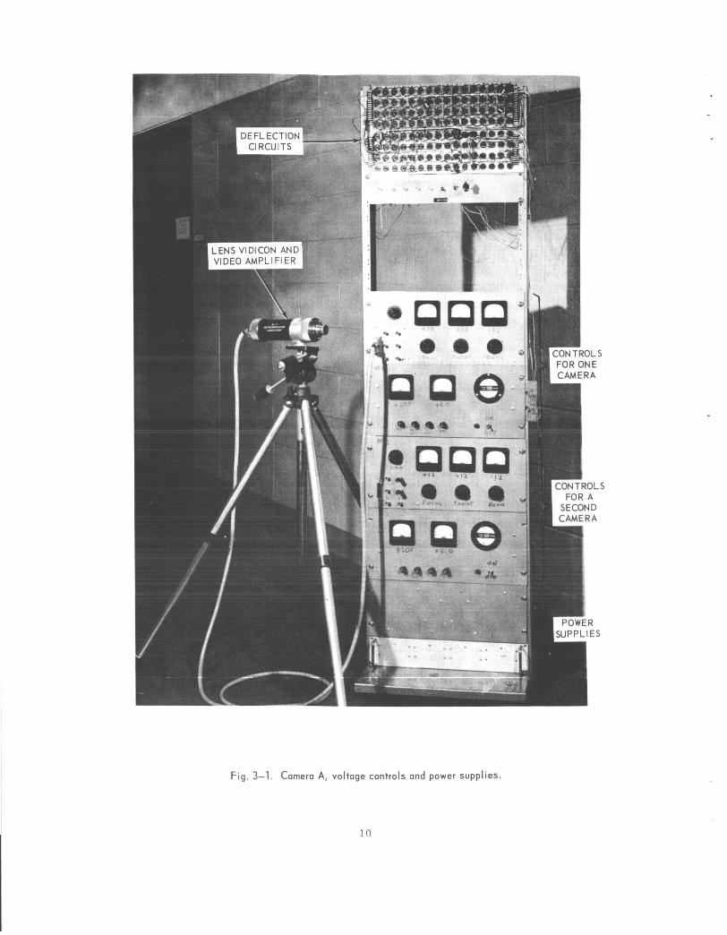
F i g . 3-1. Camera A, voltage controls and power s u p p l i e s .

10

l -

I -

l l

3. 4 Experimental Camera C

A new camera, called Model C, w i l l replace the Model A and be employed in Camera Assemblies C and D. bandwidth, DC-coupled blanking during flyback, and an increase in f rame rate f rom 1 f rame/3 sec to 7 f rames/sec due to better integration of the camera with the A-D converter and computer.

3. 5 Experimental Camera Assemblies B, C, D and E

Advantages of the new camera include greater

Experimental camera assembly B was planned to include two cameras , both looking at the same scene through a beam splitter, one having a fast response and the other slow. should be able to detect motion. the frog's retina!') It is not stereoscopic at present.

By comparing the outputs of the two cameras, a computer Such a scheme is shown in a proposed model of

Experimental camera assemblies C, D and E will be stereoscopic; that is, light will enter along two axes separated by a distance either equal to o r greater than that between the human eyes. a s tereo head on a single camera. strated by motion pictures taken through the s tereo head.

axes in a s te reo head a r e parallel, the field of view is fairly wide (25") and the resolution on the face of the camera tube poor. the single camera with i t s s tereo head will be replaced, in camera assembly D, by two cameras having narrow acceptance angles and capable of convergence. Each camera can turn through 35", as shown in Fig. 3-3. the two cameras can nod through an angle of 30" .

Camera assembly C (Fig. 3-2) will employ The utility of such a system has been demon-

Since the two optical

To improve this resolution,

The case supporting

Camera assembly E is at present an objective: an assembly much more

compact than assembly D, it is mounted on three gimbals, the outermost of which wi l l be attached to a vehicle.

3 .6 Visual Decision Computer

Figure 3-4 shows how a visual decision computer may determine what is the most likely object observed or pass the question on to the system decision computer. free-standing objects, their range, the i r texture, etc. f rom the visual decision computer indicate degrees to which certain properties a re present. Simple properties may indicate the probabilities that they repre- sent different objects. Complicated properties may be formed into object pro- babilities at a la ter stage, namely, at the system decision computer, which wi l l command a small number of corresponding acts.

The output of the visual, f i rs t -s tages computer is the outlines of The analog output lines

11

VIDICON TUBE

Fig. 3- 2. Camera and Stereohead StereoHead Assembly C as Originally Conceived. Camera A Shown here will be replaced by Camera C.

AXES OF ROTATION

d OFCAMERAS

Fig. 3-3. Camera assembly D.

12

c ?

TV CAMERAS

c

Fig. 3-4. Use of a decision computer in the visual subsystem of a robot.

w

c

c c c

of the - -Visual --C -1rnoges-

VISUAL Properties VISUAL - DECISION COMPUTER . FI RST-STAGE

COMPUTER

c c

Approximately 15 c analog lines - giving degrees to

hid, certain

13

SECTION 4

VIDICON CAMERA DEVELOPMENT AND INVESTIGATION OF SOLID-STATE SENSORS

by

Richard Catchpole, David Tweed and Louis Sutro

4. 1 Camera A: Choice of Vidicon and Design Description

The fast -scan vidicon camera built for experimental camera-computer chain A was designed at the Lincoln Laboratory, M. I. T . , t o provide a f rame time of approximately 1/30 sec, under the constraint that the dwell t ime each position in the r a s t e r fications, a r a s t e r s ize of 6 4 X 256 (sl. 6 X 10 ) positions was used.

quency at which the electron beam advanced was 500,000Hz, the dwell time.

* at **

was to be at least 2 psec. T o allow for these speci- 4 The fre- *** the reciprocal of

As plans for camera-computer chain A developed, a la rger raster s ize of 4 256 X 256 (Z6. 6 X 10 ) positions became desirable.

time constraint, this fourfold increase i n raster s ize implies a fourfold increase , in f rame time, which in turn necessitates a fourfold drop in the lower limit of

amplifier frequency response.

Given no change in the dwell

To meet this requirement, the vidicon amplifier was modified and the fast- scan vidicon was replaced by a slow-scan vidicon. vidicon was aided by the experience of J P L in using this tube on both their Mariner IV Mars fly-by" ')and the Surveyor lunar landing craft.

The choice of a slow-scan

Although vidicons magnetically deflected and focussed may have 30 percent higher resolution than their completely electrostatic counterparts, the la t ter have greater versatility in scanning rate and simplicity of circuitry. well as the design of presently operating equipment, recommended, at least

This, as

*The dwell time: The t ime the vidicon electron beam spends at each position. **Raster: The pattern produced on the face of the vidicon tube.

***Hertz: The recently adopted international unit for cycles per second.

14

in the initial experiments, that electrostatic focussing and deflection be used. Although, in our case, the coupling to the deflection plates was poor, these modi- fications made possible the motion detection experiments t o be described in a subsequent report .

4 . 2 Choice of Supplier

Because of satisfactory previous experience with their products, General Electrodynamics was selected as the supplier. This company offers a series of slow-scan electrostatic vidicons ranging in increasing ruggedness f rom a slow- scan version of the 7522 (to be denoted TD 1343-018) , through the TD 1347, to the T D 1343-010 designed for the Mariner missions. supplied with a black level reference and fiducial(reference) markings on its face. The TD 1343-018 (approx $2,000) appeared adequate for laboratory use, given a dark reference generated by blanking the vidicon during the line flyback.

4 . 3 Method of Scanning

The latter is normally

The existing deflection counter system (Ref. 1 1 1 when clocked a t a constant r a t e by the computer, was considered adequate t o provide fly-back blanking and end - of -frame signals.

4 . 4 Vidicon Circuitry

Due to the published limiting resolution of electrostatically deflected and focussed vidicons, there was no point in planning for more than 512 samples per line o r lines per frame.

It was decided, a s an interim measure, that the video amplifier used in the Lincoln Laboratory DITS system could be modified t o meet the requirements given in subsection 4 . 1 and that optimization of the high frequency cut off, re- quired for a r a s t e r measurement of 512 X 512, would be attempted later. basic modification included the increase of the target load resistance permitted by the decrease in importance of high frequency response. The front end of the video amplifier is of excellent low noise design. provided the black reference, order of magnitude.

4. 5 Improved Deflection Amplifiers

A

Blanking during line flyback Al l coupling capacitances were increased an

For the experimental vidicon camera system, a more reliable deflection amplifier was developed to replace that reported in Ref. 11.

static vidicon tube, the deflection electrodes a re arranged in pairs which deflect the electron beam in mutually perpendicular directions. pair is driven by a deflection amplifier with symmetric output voltages.

typical tube, the General Electrodynamics 7522, requires a mean deflection plate

Within an electro-

(See Fig. 4-1. ) Each A

15

potential of 200 v to 250 v and a potential difference between ei ther pair of up to

60 v. from digital-to-analog converters. Continuous horizontal deflection is effected

For digital deflection, the amplifiers a r e driven by low-level voltages

Fig. 4-1. Vidicon deflection system.

The modified Darlington deflection amplifier (Fig. 4 - 2 ) uses available volt- Symmetrical age supplies and is coupled to the deflection plates by capacitors.

negative feedback improves linearity and stabil izes gain. and zener diodes provide the mean plate voltages. 2 Fsecs, a satisfactory value for this experiment.

4 . 6 Operation of Camera Under Computer Control

The connection of one of the digitally-controlled cameras to M. I. T. ' s TX-0

Chains of res i s tors The amplifier rise time is

computcr permitted an experimental study of motion detection.

1 6

~ * - , .

A

24K 1w

SYMMETRIC

13V

INPUT

ov

RESISTORS: V8W UNLESS SPECIFIED OTHERWISE RESISTOP PAIRS MATCHED TO 2%. DIODES: 1N914 TRANSISTORS: 2N871

Fig. 4-2. Vidicon deflection amplifier.

The capabilities for data-acquisition of the M. I. T . TX-0 computer and i t s availability during recent months :ommended its use on a t r i a l basis for experi- menting with and demonstrating visual data acquisition, reduction of visual data t o information, and information-processing.

1. 7 Soiid State Sensors

Visits to Westinghouse’s Defense and Space Center, Aerospace Division, Baltimore, Maryland, filled in details of published reports (12’ 13)on the only

two-dimensional a r r ay of phototransistors now available. t ransis tors is being considered because of i t s smaller s ize and the discrete position of i t s photosensitive elements. the variation of gamma (see below) over individual units is unknown. reason, we have decided to defer procurement of an a r r ay until presently- planned tes ts have been made of the gamma of a representative phototransistor s ample.

An a r r a y of photo-

However, i t s resolution is poorer and For this

The gamma of a sensor can be defined a s the power to which illumination ( 1 4 ) must be raised in the equation for signal-output current:

7 i = k E

17

where i is the signal current, k is a constant, E is the illumination on the face- plate of the vidicon, and y is the exponent commonly referred t o a s the vidicon ganima. If the gamma of all phototransistors in an a r r a y were the same, o r if their outputs were to be communicated to Earth, there would be no concern. In the latter case, the gamma of each element of the a r r a y could be stored in the Earth computer and used to normalize the returns before interpretation. ever, since the goal is t o interpret at the remote location through the use of a light portable computer, it is not likely that a large number of gamma values can be stored. on -site computations.

HOW-

Only if gamma is uniform over the a r r ay can it be employed in

18

SECTION 5

T H E DECISION SUBSYSTEM

by

William Kilmer, Jay Blum and David Peterson

5. 1 Goal

The goal of the work described in this section is the design of a decision computer for a robot. Such a computer should be capable of e i ther interpreting what is the object that h a s been viewed by the visual system in t e r m s of a small number of possible corresponding acts o r deciding what is the most likely act that the robot should perform in response to not only visual but to all inputs.

Eventually two computers may be developed to handle each of the two require- ments, although, for the present, one is being designed that is sufficiently general to handle the needs of both.

A decision computer is used both to interpret objects a s described in sub- section 3. 5 and to decide, a s described in subsections start ing with 5. 4, what is the most likely act the robot should perform.

5. 2 Previous Descriptions

The decision computer was originally described as a model of that part of (15,161 the animal nervous system known as the core of the ret icular formation.

The model represents the spatia1,not the temporal properties of this formation and is therefore called S-retic. structure, the long-range design goal w a s to make it a functioning engineering system such a s that described in 5.1 above.

While it began as a model of the biological

19

5.3 Simulation

The design of the computer consists of the analysis presented in this section and simulations performed on the Instrumentation Laboratory general-purpose digital computer. 1965. model converged to the correct act in each of about 50 tes t cases, and always in from 5 to 25 time steps.

5.4 Computer Design

The first successful simulation was achieved in December Further simulations made it possible to adjust parameters so that the

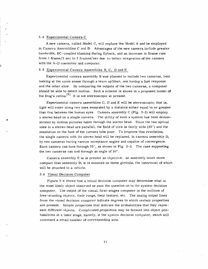
The computer logic resembles a stack of poker chips (Fig. 5-1). Each poker-chip region, Mi, is a hybrid computer module which will be described in two stages. input -output connections shown in Fig. 5-2. with more detailed illustrations.

To understand the operation in general it i s sufficient to see the Detailed operation will be described

The decision subsystem is intended to act like an admiral who commits the ships and aircraft under his command to one act, trusting that fine perceptions and fine control are made at their centers of specialty and a r e accurate. The subsystem is thus broad in the domain of i t s command but exceedingly shallow in any specific area. information that has played upon it in the last minute o r so. After commanding the robot to an act (for example, advance, turn right, turn left, right itself, per- form an experiment, etc. ) it w i l l send out directives t o control centers, tuning them to this task.

It w i l l commit t h e robot t o an act which is a function of the

I t s important features a r e that it must handle a vast amount of highly cor- related input information and arr ive at one of a small number of mutually ex- clusive acts in a dozen o r s o time s teps and with minimal equipment. crucial information a s t o what act the system has selected will then be used to control the inputs so a s to increase the probability that the act w i l l be continued.

The

In Fig. 5-1, the 4 2 input lines, yi, a r e connected to the modules in a several- to-all, but not all-to-all, fashion, A model of this environment is established by factors, a i , of the set Z.. The Si represent sensors of this environment which feed highly (but nontrivially) cor- related inputs, y., directly into the decision system. U. and y . lines a re binary.

The outer box represents the environment.

At this stage of design, all 1

1 1

There a re twelve logic modules in the present design. The se t s of lines pi

There a r e four The four

(only P7 is marked) indicate the act preferred by module Mi. lines in each set because the model is at present capable of four acts. lines carry t h e four components of a probability vector.

213

Fig. 5-1. Simulation of the decision subsystem.

For clarity, all types of connection lines ( E P, ascending and descending lines) a r e shown only for module M,, whereas these types of connection are ac- tually made to all regular modules. not all S., and each S. feeds several but not all Mi.

5. 5 Operation in General

Each M. receives inputs from several but 1

3 3

Each module (Fig. 5-2) computes directly from the input information it receives and makes a best guess as to what the corresponding act probably should be. After the initial guess, the modules communicate their decisions to each other over low capacity information channels. Then each module takes the in- formation (from all other modules) and combines it in a nonlinear fashion with the information coming directly into it to a r r ive at a mixed guess a s to what act

2 1

ti-

\

v) W

? 2

should be performed. which it is connected above and below. Thus we have decomposed the msdule shown in Fig. 5-2 into two parts. The A part operates on the module's input information. The B part operates on information from above, below and frorp the A part.

This is in turn communicated to the subset of modules to

The A part with five binary input variables and four analog output variable outputs, is a nonlinear probability transformation network.

The B part receives 4-component probability vectors P6 from the above, Pa f rom below and PAB from the A part. The j th component of each probability vector is the probability, computed by the module of origin, that the decision sys -

t em ' s present y input signal configuration demands act number j .

also receives the difference between y inputs, called I'y difference" in Fig. 5-2 and the strength of convergence Q, shown being formed in the lower right corner of Fig. 5-1. The B part of each module yields the probability that the decision system's present y input demands act number j .

The B part

The design of the modules was straightforward. The main problems con- cerned the way in which the computation converged to produce consensus.. This concensus is achieved, a s illustrated in Fig. 5-1, by f i rs t determining at point s i f the jfh component of the probability vector P from each module exceeds 0.5. If it does, a 1 is passed on to the threshold element T . .

J jth component input connections a r e l ' s , act j is decided upon. Note that each element T . in Fig. 5-1 receives 10 inputs, although for clarity of the drawing, connections a r e shown only to T3. of a motor control subsystem which receives many inputs, decodes them and commands an act.

There, if 60% of the

.I Each threshold element T is a crude model

5. 6 Definitions

A concept of importance in the decision system is that of the probability vector. possible responses, is an n-component vector H = (p 1, p2, . . . pn). Its jth aom- ponent, P., represents the probability that the th response is the appropriate one. probability is 0. 15 that response 3 is the appropriate response.

A probability vector, associated with a decision for which there a r e n

3 F o r example, in the probability vector P1 = (0. 35, 0. 10, 0. 15, 0. 40), the

A normalized probability vector is one representing mutually exclusive and collectively exhaustive responses; the components of such a vector thus sum to 1. can be represented:

The vector F1 in the example above is a normalized probability vector which

n - P I = C pi =(0.35 tO .10 t 0 . 1 5 t0 .40 ) = 1.0

i l l

23

In the present decision system, we consider 4 different responses, o r acts; hence the probability vectors used in this report have 4 components.

A - flat probability vector is one whose components a r e equal. A mean pro- bability vector is a flat probability vector whose components a r e normalized. general, the mean probability vector can be represented a s

In

- Pm = (1/n, l / n , - * * , I/n)

-,-'

n e l e m e n t s

'The vector P2 = ( 0 . 3 , 0. 3, 0. 3, 0. 3) is a flat probability vector while P3 = (0. 25,

0 . 25, 0. 25, 0. 2 5 ) i s a mean probability vector.

The peakedness of a probability vector P is a function proportional to the difference between P and the mean vector pm. of vector P = (p l , . . . pn) i s

One definition of peakedness K

2

K = 2 (Pi-;) i = l

Other definitions of "peakedness" a r e used to meet the requirements of a par- ticular case.

5. 7 Detailed Operation

Given only its limited view of the environment, each module M . (i = 3, 4, . . . 1

12 in Fig. 5-1) computes, during the first time interval, the initial guess de- scribed i n subsection 5. 5 .

all modules have made such computations, they communicate their respective Pi's to each other over the low-capacity a- and 6-information channels (a and 6 in Fig. 5-1). During the second time interval, each module combines in a nonlinear manner its own sense information about the environment with information coming into it from other modules to arr ive at a finer-probability vector ("mixed guess" in subsection 5. 5 ) .

the third time interval, a yet-finer probability is computed. operates in cycles until the modules reach general agreement, o r convergence.

This is the normalized probability vector Pi. After

This vector is communicated t o the other modules, and during The system thus

At the completion of each cycle, the Pi output of each module is examined at

T4. If the j th component of s and then passed to the threshold elements T

Pi exceeds 0. 5, the s passes a 1 to T . . At T . , if

60% or more of the inputs a r e l 's, then act j is decided upon. When an act has been selected, the box labeled "strength of convergence'' sends back a Q signal to the modules. where z is the act decided upon. decoupling the modules from each other.

1 . . - Otherwise, s passes on a 0.

3 3

This signal i s proportioned to the number of 1's received by TZ, Q prepares the modules for a new input by

24

After a decision is reached, the system receives new 2 = (0, . . . a,,) and the ent i re decision process is repeated. number of cycles, the system is reset and a new L: requested.

If no decision is reached after a certain

Now that the decision system has been described, the internal structure of a module will be considered in detail.

5. 8 Structure of a Module

There are two types of modules in the decision system. Modules M3, . . . M12 are "regular" modules. Modules Ml and M2 a r e "upper-lower" modules.

A s previously explained, the regular module illustrated in Fig. 5-2 is divided into two parts. The A-part calculates a normalized probability v e d o r PAB based upon the y-inputs. The R-part produces a normalized probability vector fii as a function of both pAB and the probability vector Fa and F6 f rom the other modules' B-parts.

-

The upper-lower modules consist of only A-parts, Their vector outputs FAB arc distributed over a- and 6-lines t o other modules, but a r e not used directly in making a decision.

The A- and B-parts are discussed separately in the following paragraphs.

5.9 The A-Part of Each Module

The A-part has two tasks, One is to determine when and by how much the

input y ' s change. y ' s f rom the previous cycle. The parameter C, is computed to be proportional to the number of y ' s that have changed since the previous cycle. Hence CT1 is large when the outside world is changing dramatically, and small when the out- side world is remaining essentially stable.

At the s tar t of each cycle, the new y ' s a r e compared with the

1

The second task of the A-part is to calculate a 4-component normalized probability vector PAB based upon the y-inputs f rom the senses. simulation of the nonadaptive decision system, the A-part is simply a tabular listing of r - to-PAB correspondence. to represent situations in which the decision system has to make a choice. One

possible adaptive A-part structure using threshold logic is presented in Appen- dix A. me mor andum.

5.10 The B-Part of Each Regular Module

In the computer

The correspondences used were selected

Another structure, using table-updating, will be presented in a subsequent

Only the ten regular modules contain R-parts. Figure 5 - 3 shows the internal

s t ructure of each B-part. andPABi from the corresponding

A-part, F6 f rom modules above Mi, Pa f rom modules below Mi' and Q from the i

The inputs a r e C "1

25

I LLI U

1 ti- - w U Z w u LLI

I I I I

4 Z

4 4 4

2 6

"strength of convergence". In general, each component of P6. comes from a different module; similarly Pa,.

1

1

Each of the boxes labeled "N" is a normalizer whose output is a normalized probability vector with components proportional to the corresponding components

of the input probability vector. The boxes labeled "f" have the t ransfer charac- ter is t ics shown in Fig. 5 - 4 . The boxes labeled "P" calculate the peakedness of the respective input vector without changing the vector itself. Ca is the peaked- ness of the normalized P and C6 the peakedness of the normalized P6,. ai

0.05

1

1.0 - INPUT

Fin 5 4 The f funrtion. . ,J. - .. . .

The averaging mechanism in Fig. 5 - 5 combines the PAB? pa, and P, in a weighted average as follows:

27

Pi

,

1.6

1.4

1.2

0.f

0.L

/ /

/ / -

0.4 0 8 1.2 1.4 1.6

Fig. 55. h(pi) and h-' (pi).

The preferences f rom the A-part of the module will be given more influence

l'lic preferences f rom the module above o r below Mi will be given i n determining F! when C

dramatically. inoi-c' ini'liiencc. whcnT6 o r Ha arc very peaked.

is large, i. e . , when the outside world is changing 1 "1

In gene ra l P! is not a probability vector in the t rue sense because the com- I'onents of p! a r c not d l : 0. P! must be restored to a probability vector while preseri+ng the relative significance of the components. A single l inear shifting of the coriiponents by adding an appropriate constant t o each of them would yield a vector with positive components, but the relative meaning would be distorted, since tiiffcrenw between small pro1)al)ility components (e. g. , between 0. 2 5 and 0. 05) :ire m o r < % significant than the same differences in magnitude between large

1

probability components (e. g., between 0. 65 and 0. 85). componentwise, through an exponential function, h, a s shown in Fig. 5-5. these components a r e linearly shifted into positive value in the "T" box (Fig, 5-3) by adding to each component the absolute magnitude of the most negative component. The resul ts of the shifting are then passed componentwise through the h - l curve (Fig. 5-5) and normalized at N, resulting in the module's output vector 9. delay.

Hence Fi is f i r s t passed, Then

This is sent to specified modules above and below Mi after a unit

29

SECTION 6

CONCEPTUAL MODEL O F THE FROG'S TECTUM

by

Roberto Moreno-Diaz

6. 1 Introduction

The model of a f rog 's visual system described in previous has

been extended to include a model of the tectum.

Figure 6-1 is a diagram of the frog 's visual system with the eyes enlarged so that the ganglion cells can be illustrated collecting information from the retina and conveying it to both the optic tectum and the geniculate nucleus. tions t o the tectum a r e the principal ones. presence of blue light in the field of view is reported t o the geniculate.

Connec-

Experiments indicate that only the

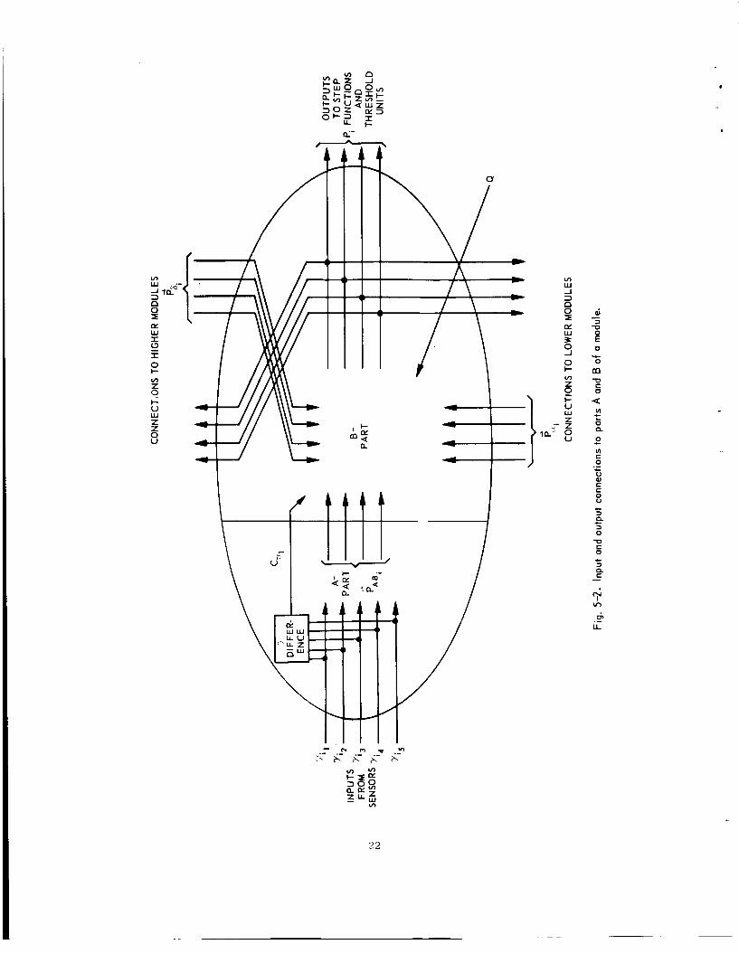
Figure 6-2 represents schematically the retina and optic tectum. The

retina consists of three layers: The photoreceptors, which respond to light, st imulate the bipolar cells, which in turn stimulate t h e ganglion cells, whose axons, or tails , comprise the optic nerve. separate layers of the tectum. Each type of ganglion cells performs a different analysis of the retinal image and reports, through the optic nerve, to the tectum, in the following manner:

photoreceptors, bipolar and ganglion cells.

The axons of each of four kinds of ganglion cells terminate on four

1. Group 1 ganglion cells respond to edges, i . e . , to differences in illumination on the receptive field,

Group 2 ganglion cells respond t o the image of a small dark object, moving centripetally into i t s visual field.

Group 3 ganglion cells respond to any change, spatial o r temporal, in the luminance of the scene.

Group 4 ganglion cells respond to dimming of light.

2.

3.

4.

Lettvin, et al. have found correlation between the fo rm and function of each ( 1 7 ) of these cells.

Their description of the tectum has not been as thorough, however, since they were concerned only with the response of tectal cel ls in an animal acquiring

30

STEM

Fig. 6-1. Diagram of frog’s visual system.

GROUP NO. OF GAPiGiiON C E L L

TERMINALS

, ! 2 - RETINA I I i:

5 x 105 GANGLION CELLS

\ IO6 PHOTORECEPTORS

lo6 BIPOLAR CELLS \ 2.5 x 105 TECTAL CELLS

Fig. 6-2. Schematic of frog visual system.

31

food(17) Nevertheless, t1ieii.s is the only description of tectal behavior suitable

to be considered in o u r model.

6 . 2 Neurophysiological Basis of the Model

Pedro Ramon y Cajal's drawing of the frog's tectum is shown in Fig. 6-3 .

Although the drawing is not cor rec t in detail, there are four main features that

-

Fig.6-3. Pedro Ramon y c a i a l ' s drawing of optic tectum in the frog.

3 2

.. appear clearly. 6 - 3 ) .

axons leave the tectum branching from a main ascending dendrite. Fourth, interconnections among cells lying at the same depth is strongly suggested.

F i r s t , the cell bodies lie in the deeper layers (1 to 6 in Fig.

Second, the neurons seem to have a restricted dendritic t ree . Third,

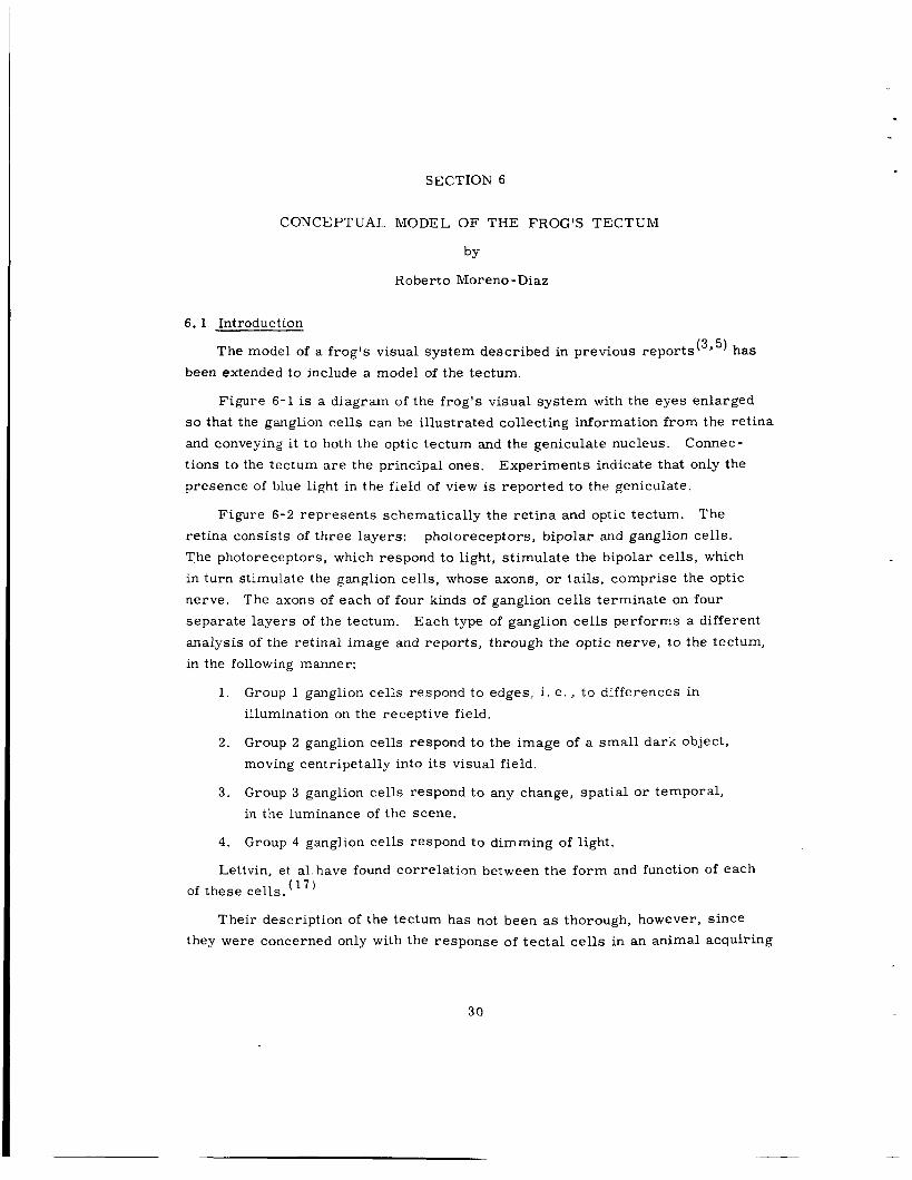
Figure 6 - 4 adopted from the discussions of Ref. 1 7 shows what appear t o Axons from the four major be the essential anatomical features of the tectum.

retinal ganglion cell groups enter the tectum as the optic t ract and map onto the four superior tectal layers called the superficial neuropile.

lion cells which respond to adjacent retinal a r eas map onto adjacent points in the neuropile. T h u s , each small a r ea in the retina corresponds to four small a r eas ,

one on each layer, in the neuropile. cells - not represented in the figure - which appear to be la teral connectives.

Axons from g a g -

Within the neuropile there also exist a few

TECTAL CELL

I TERMINATIONS OF GANGLION CELL AXONS

*&+=-

Fig. 6-4. Simplified diagram of frog’s tectum.

3 3

All other tectal cell bodies lie in the granular layer, beneath the superficial

neuropile (Fig. 6 . 3 ) . Their dendrites, which have the appearance of columns, extend up through the four neuropile layers covering a smal l a r e a in each layer. Their axoris leave the tectum by branching from the main dendrites, at the lower part of the neuropile.

A R E A K

DENDRl TES

L A Y E R 1

L A Y E R 2

L A Y E R 3

L A Y E R 4

* Fig. 6-5. Diagram of a tectal neuron.

Lettvin, et al.have distinguished from several varieties of tectal neurons two extreme types: "Newness" cells, N, sensitive to new Objects in the visual field, and the "Sameness" cells. S, sensitive to the same object for a specific period of time. The bodies of Sameness cells lie deep in the granular zone.

The properties of Newness and Sameness cells a r e shown by the following out line:

a . Newness Cell

1. Its receptive field is approximately 3 0 " in diameter, with considerable overlap.

It yields smal l responses to sharp changes in illumination. 2 .

34

3 . Its response frequency increases if the motion of an object is i r regular . Its response also depends on the velocity and s ize of the object and on the direction of motion.

It has no enduring response.

Its adaptation time is less than 1 second.

Adaptation is erased with a step to darkness.

4.

5.

6 .

b. Sameness Cell

1. Its receptive field is almost all the visual field, but includes a null region.

It does not respond to changes in illumination.

It responds to the presence of an object in its field by generat- ing a low frequency pulse train. objects about 3 " in diameter.

T I "notices" with a "burst" of pulses all motion discontinuities.

It discriminates among objects, fixing its "attention" on the one with the most irregular movement.

2 .

3 . Response is maximum to

4 .

Lettvin, et a1,comment that N and S cells may be considered two extremes From Pedro Ramon y Cajal 's drawings, tectal of several types of tectal cells.

cells do not seem to be significantly different, anatomically, although S cells could receive excitation from N cells. visioned, in which N and S cells would be differentiated only by values of param- e t e r s , such a s adaptation time, width of the receptive field, etc. point of view adopted here.

A general tectal model could be en-

This is the

While the receptive field is relatively wide for both types of cells, the den- dr i t ic t r ee is very restricted. this observation.

Interaction between tectal cells would account for

6 . 3 Conceptual Model

In the conceptual model of tectal-cell behavior, object velocity and size is determined by signals assumed t o originate on the retina. current and voltage signals a r e referred to simply a s "activity".

F o r convenience these

Assume that each layer of the superficial neuropile is divided into small areas , such a s a rea K in layer i (i = 1, 2, 3, 4). cell axons of Group i map into this area and emit their signals there. decoding process which produces analog values such a s voltage signals.

V map into a rea K of layer i.

(See Fig. 6-5 . ) Some ganglion- Assume a

Let (t) be the voltage signal indicating the response of the ganglion cells which iK

35

Assume fur ther that t h e dendrites of each tectal neuron a r e res t r ic ted to an The f i r s t process t h a t i s suggested is a a rea K - i. e . , there is no overlapping.

summation of the signals, ViK(t), for the same K and different i ' s at t ime t . simple linear combination is postulated:

A

The coefficient aiK may be either positive or negative and i s assumed constant. If it is positive, the corresponding ViK(t) is said to he excitatory; i f it is nega- tive, V. (t) is said to be inhibitory. a

transmit signals V (t) through the superficial neuropile. due to the conductivity of the medium through which they pass.

aIK, a2K and a3K a r e positive, whereas i K is negative. By summation(') a series of "vertical" lines i s obtained, which

These s i p a l s interact 4 K

K

Four interaction processes account for tectal cell properties. (See Fig.

6-6.) axons, are of the same nature - i. e. , an interaction due to the conductivity of the medium. existence of a distributed capacity which, once charged, damps the transmission of t h e signals J'rocess C' requires non-symmetric elements (e. g . , diodes) that could be provided by the cellular me:nbrane. These processes a r e described in

Process A at the level of the dendrites, and Process D, at the level of the

Process B,which accounts for adaptation, may be produced by the

niore detail in the following subsections.

6. 4 Interaction Process .4 (Facilitation)

Lateral sprcading of activity increases the response to an i r regular ly moving object. fore interaction. according to a continuous and decreasing function f(d f -+ 0, d +-. It is further assumed that the effects of different l ines on a particular one add linearly, Therefore, the final activity (i. e. , activity after interaction), Vt((t), is:

V,(t) is referred to as the initial activity of line k, i. e . , the signal be-

kJ Its effect on another line J depends upon the distance d

); f(d kJ kJ ) is such that as

This effect propagates with a velocity, y , assumed to be constant. kJ

where the s u m is over all lines except I< . If f (0 ) = 1, Eq. ( 2 ) becomes:

V ' ( t ) = v. ( t - - ';J) f(dki) K J

where the sum is over all lines, including k

36

PROCESS A

PROCESS B

* CELL = OUTPUTS f

.. EXCITATION

D DISTRIB. D e- D - -- * - - - PROCESS 0

t

I A 1 , ' I I * MAX. ACT.

C

r

.. PROCESS C - - - SELECT0 R * C c -- c .

Fig. 6-6. Diagram of tectal cell interaction processes.

Lateral coupling is assumed for Type N neruons over a zone covering 30' of the visual field; for Type S, over the entire visual field.

Figure 6-7 shows an example of the results of this interaction for an object following a straight path. t h e summed voltage wi l l be greater for objects that change their direction of motion.

6. 5 Interaction P rocess B (Adaptation)

P rope r capacitive coupling will cause a line that has been excited t o adapt

The distribution of equipotential activity shows that

and damp any further transmission for some time.

described in subsection 6 . 8.

Appropriate capacitors a r e

37

EQUIPOTENTIAL LINES OF FACILITATION

MOVING IN A STRAIGHT

LINE

Fig. 6% Facilitation for an object fallowing a straight path.

6 . 6 Interaction Processes C and D (Maximum- activity selection and distribution)

Process C blocks all paths except the one having maximum activity, and P rocess D distributes this activity to the other lines, in a manner s imilar to

P rocess A. stand how these processes can be realized. each with a voltage Vk(t) connected through an ideal diode represented by a diode in a circle in Fig. 6-8. Currents flow through axonal r e s i s to r s Rax, f rom the Vk(t) with the highest value. type of interconnection exists will follow that with the highest activity. VI (t) with highest value will appear to ”govern’l the others. objects in the field of view corresponding to the zone in question - i. e . , two generators with a high value - only that which produces the higher V k ( t ) w i l l be followed.

The following circuit analogy provides an example that helps under- Assume a number of generators,

rp

Neurons belonging to the zone where this Thus, the

If there exist two K

If it is now imagined that some coupling r e s i s to r s exist (indicated by dots in Fig. 6 - a ) , the action of V‘ ( t) w i l l be attenuated with an increase in the dis- tance from the a rea that produces it. object in the field of view will be maintained in the RC circuits.

6 . 7 Parameters of Types N and S Neurons

With lateral coupling for Type N neurons assumed for a zone covering 30

K Information concerning the position of the

of visual field, necessary capacitive time constants for adaptation a r e such that damping of signals occur in 1 second and persist for 50 t o 70 seconds. The

*‘The output of the tectal cell, K, could be regarded as a pulse t ra in of a f r e - ax, K’ quency proportional to the current through R

38

difference between the t ime required for adaptation and the t ime for e ra su re of

adaptation is a consequence of the nonlinear elements (diodes) that cause Pro- cess C, i f we assume that they a r e real diodes; i. e . , they have a finite, although high, backward resistance. action P rocess C a s long as the backward resistance is o rde r s of magnitude higher than Rax. whereas VqK is negative. ness - Le., strong firing of Group 4 ganglion cells - the capacitators are then discharged through the backward resistance of the diodes.

This assumption will not modify appreciably inter-

As stated in subsection 6.3, VlW VZK' and VQK a r e positive As a result, adaptation is e ra sed by a step t o dark-

Fig. 6-8. Equivalent circuit of Processes Jl l and N.

For Type S neurons, V (t) is made higher by the addition t o the signals K coming from the retina of the output of some Type N neurons. la teral coupling occurs over almost all the visual field. implying a high value for the adaptation capacitance.

6. 8 Equivalent Circuit of a Group of Tectal Cells

The circuit analog of a group of either Type N o r S tectal cells is shown in

For Type S cells Adaptation i s negligible,

Fig. 6-9. The group includes only those cells which are situated at the same level i n the granular layer. CK is the equivalent capacity for adaptation. D is a real diode. Interaction among the axons of neurons belonging to the same group is indicated by r e s i s to r s RC. firing of a cell is considered to be proportional to (Iax,K - OK), where Iax,K is the current through Rax,K and 8, is a fixed threshold. some cells can be explained by assuming an assymetric distribution in the values of the coupling resistances R

Process A is not indicated.

r, K The r a t e of

The directionality of

C '

39

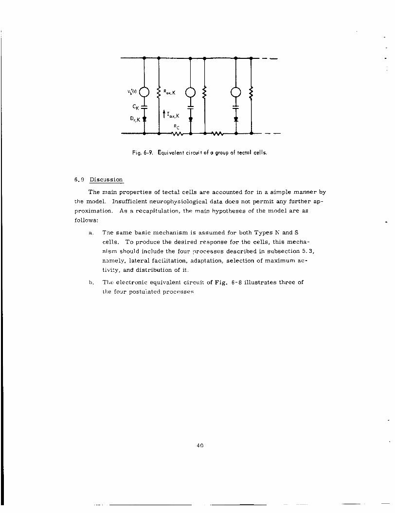
Fig. 6-9. Equivalent circuit of o group of tectal cells.

6.9 Discussion

The main properties of tectal cells a r e accounted for in a simple manner by the model. proximation. follows:

Insufficient neurophysiological data does not permit any further ap- A s a recapitulation, the main hypotheses of the model a r e as

a. The same basic mechanism i s assumed for both Types N and S cells. nism should include the four !x-ocesses described in subsection 5. 3, namely, lateral facilitation, adaptation, selection of maximum ac- tivity, and distribution of it.

TILe electronic equivalent circuit of Fig. 6-8 i l lustrates three of the four postulated processes.

To produce the desired response for the cells, this mecha-

b.

4 0

APPENDIX A

NOTE TO SECTION 4: IMPLEMENTATION OF THE A-PART O F A DECISION-SYSTEM MODULE USING THRESHOLD LOGIC

Figure A-1 is a schematic diagram of an A-part using threshold logic. The

can be either ek a r e l inear threshold logic elements. positive or negative. F o r threshold a . is

The gains, o r weights, a . the output vik of threshold element ek

Jk

J k '

Each f l in Fig. A - 1 is a summation element whose output is

PABl 2 w k l "ik k = l

This threshold and summation logic approach can incorporate learning through the reinforcement of the weights a . O ~ U L L the c n v i r c ~ m e z t .

and wkl a s a result of rewards fed Jk

7 - 7 - r.--

"Thus, vik is equal t o 1 when the sum of each of the inputs 7 . . t imes i t s respec- tive weight aik is equal to o r greater than the threshold a. l3 Otherwise V i k is equal t o 0.

41

yi 1

yi 2

Yi 3

Yi 4

Yi 5

'AB

'A02

Fig. A-1. Threshold logic implementation of the A-port of module i.

42

LIST OF REFERENCES

1. Sutro, L.L.,Moulton, D. B., Warren, R. E. , Whitman, C. L., Zeise, F. F . , 1963 Advanced Sensor Investigations, R-470, Instrumentation Laboratory, Massachusetts Institute of Technology, Cambridge, Massachusetts, Sep- tember, 1964.

2. Sutro, L. L., editor, Advanced Sensor and Control System Studies, 1964- September, 1965, R-519, Instrumentation Laboratory, Massachusetts Institute of Technology, Cambridge, Massachusetts, January, 1966.

Missions, R-545, Instrumentation Laboratory, Massachusetts Institute of 'Technology, Cambridge, Massachusetts, June, 1966.

3. Sutro, L. L., Information Processing and Data Compression for Exobiologv

4. Mahoney, J. J., Data Transmission Capabilities of Wars Probes and Landing Capsules, American Astronautical Society, Anaheim, California, May 23- 25, 1966.

5. Moreno-Diaz, R. , An Anal.ytica1 Model of the Group 2 Ganvlion Cell in the F rog ' s Reti@, E- 1858, Instrumentation Laboratory, Massachusetts Insti- tute of Technology, Cambridge, Massachusetts, October, 1965.

6. Sutro, L. L., Information Processing and Data Compression for Exobiology Missions, R-545, p. 5-12.

7. Bendix Systems Division, Surveyor Lunar Roving Vehicle, Interim Study, F i n a l Technical Report, BSR 1096, the Bendix Corporation, Ann Arbor, Michigan, February 1, 1965.

8. General Motors Research Laboratories, Final Report, Surveyor Lunar Roving Vehicle, TR 64-26, General Motors Corporation, Santa Barbara, C d i f n r n i i , April 23, 1964.

9. b i d . , p. 13-15. 10. Malling, L. R . , Space Astronomy and the Slow-Scan Vidicon, Journal of the

SMPTE, Volume 72. November, 1963. 11. Sutro, L. I,. , editor, Advanced Sensor and Control System Studies, 1964 to

September, 1965, R-519, p. 61-64. 12. Schuster, M. A., and Strull, G., A Monolithic Mosaic of Photon Sensors for

Solid-state Imaging Applications, IEEE Transactions on Electronic Devices, December, 1966.

13. Broderick. J. C., and Schuster, M. A., A Molecular Camera for Aerospace Applications, 1965 International Space Electronics Symposium, Miami Beach, Florida, November, 1965.

14. Fink, D. G. , Television Engineering Handbook. McGraw-Hill, p. 1-50, 1957. 15. Sutro, L. L., editor, Advanced Sensor and Control System Studies, 1964 to

September, 1965, R-519, p. 84-95.

43

LIST OF REFERENCES (Cont.)

16. Sutro, L. L., editor, Advanced Sensor and Control System Studies, 1964 to Selstember 1965. R-519. D. 84-95.

17. Lettvin, J. Y . , et al . , Two Remarks on the Visual Systems of the Frog, Sensory Communications, W. Rosenblith, ed. , Massachusetts Institute of Technology, 1961.

18. Nathan, Robert, Digital Video Data Handling, Technical Report No. 32-877, Jet Propulsion Laboratory, California Institute of Technology, Pasadena, California, January 5, 1966.

44