1 Introduction

Despite a series of well known critiques dating at least to Allais (1953), expected utility theory

remains the workhorse framework used to analyze risky decisions. Recent applications of

expected utility range from the analysis of optimal taxation and social insurance to principal-

agent problems and portfolio choice. In the expected utility model, risk aversion arises

from the curvature of the underlying utility function, which is commonly measured by the

coefficient of relative risk aversion (γ). The conclusions drawn in any application of expected

utility theory hinge on the level of risk aversion used to calibrate the model: the optimal

rate of insurance is higher if γ is large, optimal contracts are less incentivized if γ is large,

etc.

This paper derives a tight upper bound for γ using a well-established fact from the labor

supply literature: Individuals work as much or more when their wages rise, i.e., the un-

compensated wage elasticity is (weakly) positive. The intuition for the bounding result is

roughly as follows.1 If an individual chooses to work more when his wage rises, his marginal

utility of consumption must not diminish very rapidly. If it did, he would choose to enjoy

more leisure with his higher income rather than increasing labor supply to increase consump-

tion. Since the rate at which the marginal utility of consumption diminishes determines

risk aversion in expected utility models, it follows that an upper bound on risk aversion can

be obtained using the fact that the wage elasticity is positive.

More precisely, the main theoretical result of the paper is that γ is directly related to the

ratio of the income elasticity of labor supply to the price (substitution) elasticity of labor

supply in any standard labor-leisure choice model, without any restrictions on preferences.

To see why, recall that γ ∝ uccucwhere uc denotes the first derivative of utility with respect

to consumption, and ucc denotes the second derivative. An agent’s labor supply response

1This intuition applies to the case where consumption and leisure are not complementary; the moregeneral case is discussed in detail below.

1

to a wage increase is directly related to uc, the marginal utility of consumption: The larger

the magnitude of uc, the greater the benefit of an additional dollar of income, and the more

the agent will work when w goes up. The labor supply response to an increase in income is

related to how much the marginal utility of consumption changes as income changes, ucc. If

ucc is large, the marginal utility of consumption falls sharply as income rises, so the agent will

reduce labor supply significantly when his income rises. It follows that there is a connection

between γ and the ratio of income and price elasticities.

Formalizing this connection requires an additional step. Labor supply data cannot

be used in isolation to identify cardinal properties of the utility function because data on

certainty behavior only identify utility functions up to a monotonic transformation.2 The

cardinality of the utility function must be pinned down using information on risky decisions.

To see how this can be done, observe that for a fixed degree of complementarity between

consumption and leisure (ucl), there is only one vN-M utility (up to affine transformations)

that can be consistent with a given set of labor-leisure choices. Hence, given a value of

ucl, labor supply data can be used to infer risk aversion. I show that ucl can in turn be

estimated from data on consumption choices when employment is stochastic, e.g. when

individuals anticipate being laid off with some probability.3 Intuitively, the extent to which

an agent chooses to smooth consumption across states in which labor supply differs (via

an insurance policy or saving) reveals the degree of complementarity between consumption

and leisure. Importantly, the estimates of risk aversion are very insensitive over the broad

range of values of ucl estimated in existing studies of complementarity, implying that labor

supply data itself contains considerable information about the rate at which marginal utility

diminishes .

2In other words, identification of curvature requires a 1-1 map between observed choices and γ. Inthe general labor-leisure model, such a map does not exist because any monotonic transformation of utilitygenerates the same labor supply choices.

3It is critical to have data on choices under uncertainty; barring additional assumptions, a cardinal valuefor ucl cannot be inferred from the usual certainty settings in which we typically think about estimating thedegree of complementarity between consumption and leisure (e.g. timing-of-work, household production).

2

The formula relating the labor supply elasticities to γ results in a simple and surprisingly

tight bound for risk aversion: If the uncompensated labor supply curve is upward sloping (as

found by almost all studies of labor supply), γ < 1.25.4 If γ were larger than 1.25, income

effects of wage increases would be large relative to substitution effects, creating a downward-

sloping labor supply curve. This bound rises to at most 1.66 for plausible perturbations in

the degree of complementarity between consumption and leisure. To give a better sense of

the range of values of γ that are consistent with evidence on labor supply behavior, I impute

γ using twenty-nine sets of estimates of wage and income elasticities drawn from studies

with different methodologies and data sources. In the benchmark case where ucl = 0, the

mean value of γ implied by the studies is 0.94, with a range of 0.15 to 1.45. Only one of the

twenty-nine studies finds a slightly negative wage elasticity, yielding γ > 1.25. Labor supply

data thus provide robust evidence that the marginal utility of wealth does not diminish very

rapidly in practice.

These bounds generalize to a general dynamic life-cycle model of labor supply. The

curvature of the value function over wealth — which determines risk preferences over wealth

gambles — is bounded above by 1.25 by estimates of labor supply elasticities for dynamic

models. In preference specifications where risk aversion and the elasticity of intertemporal

substitution are free parameters (e.g. time non-separable or Kreps-Porteus preferences), the

bounds applies only to risk aversion and the EIS remains unrestricted. Hence, the result of

this paper pertains exclusively to risk aversion, distinguishing it from prior work on labor

supply and the EIS in the “balanced growth” literature, which is discussed in greater detail

below.

The fact that the curvature of utility over wealth is severely restricted by behavior ob-

served in the labor market has two important implications. First, those who apply expected

4Even if the uncompensated wage elasticity were somewhat negative, risk aversion remains tightlybounded; generating γ > 2 requires an uncompensated wage elasticity more negative than any estimatein the labor supply literature to date (as reviewed in Pencavel (1986) and Blundell and MaCurdy (1999)).

3

utility theory to analyze problems such as taxation and portfolio choice must be content

to calibrate their models with a low level of risk aversion, especially in applications where

labor supply is endogenous. Second, the result implies that diminishing marginal utility

itself is inadequate to explain the high estimates of risk aversion obtained in many stud-

ies of preferences over gambles. For instance, Barsky et. al. (1997) report estimates of

γ > 4 using responses to questions about large hypothetical gambles. Estimates of γ from

portfolio choice and equity premiums exceed 10 (Mehra and Prescott 1985, Kocherlakota

1996), and estimates of γ using data on insurance deductibles are around 10 (Dreze 1987).5

A departure from expected utility theory is needed to obtain such degrees of risk aversion

without generating starkly counterfactual labor supply patterns.6

The remainder of the paper proceeds as follows. Section 2 places the result of this paper

in the context of previous calibration results for expected utility theory and the balanced

growth literature on intertemporal substitution. Section 3 derives formulas that connect risk

aversion to labor supply behavior in standard static and dynamic models of labor supply.

Section 4 gives the calibration argument and imputes γ using existing estimates of labor

supply elasticities. The final section offers concluding remarks.

2 Related Literature

The idea that labor supply data place strong restrictions on risk aversion is related to but

logically distinct from a well known result in the “balanced growth” literature, which shows

that labor supply behavior restricts the elasticity of intertemporal substitution (EIS). In

5There are, however, some studies that find very low levels of risk aversion as well. For instance, Szpiro(1986) estimates γ = 2 using data on the fraction of insured assets and Metrick (1995) estimates γ = 0 forJeopardy players.

6Even if expected utility is not the best positive model of risk preferences, having the bound on γ remainsuseful for two reasons. First, if expected utility is used as a normative model, knowing that γ is low can behelpful in determining optimal government policies (e.g. social insurance, taxation). Second, identifying γcan help in understanding which non-expected utility theory is closest to matching observed behavior.

4

a seminal article, King, Plosser, and Rebelo (1988) [KPR] show that balanced growth —

which requires constant labor supply with increasing wages — places strong restrictions on

the form of the flow utility function when utility is time-separable. Basu and Kimball

(2002) develop the KPR point further by showing that reconciling low estimates of the EIS

(as in Hall (1988) and Barsky et. al. (1997)) with balanced growth requires either strong

complementarity between consumption and labor or time non-separable utility (e.g., habit

formation).

While the EIS and γ are directly linked when utility is time-separable, they are two

distinct characteristics of preferences when utility has a more general specification, as em-

phasized both theoretically and empirically by Hall (1988), Weil (1990), Epstein and Zin

(1991), and others. This paper provides a bound on γ, without placing any restrictions on

the EIS. This point is demonstrated formally in section 3.5 by considering two preference

specifications commonly used to sever the link between γ and EIS in dynamic models: time

non-separable utility and Kreps-Porteus preferences. In both of these cases, it is shown that

effective risk aversion is identified by labor supply behavior, while the EIS remains uniden-

tified. Hence, the calibration result of this paper is purely about preferences across states

(risk) and not preferences across time periods (intertemporal substitution). Moreover, the

solutions proposed by Basu and Kimball to reconcile a low EIS with labor supply behavior

do not relax the risk aversion bound derived here.

The results of this paper are also related to those of Rabin (1999) and Kaplow (2003),

who give other calibration results for risk preferences in an expected utility model. Rabin

shows that expected utility cannot generate a reasonably high level of moderate-stakes risk

aversion without creating unreasonably high large-stakes risk aversion.7 Kaplow shows that

estimates of the income elasticity of a value of a statistical life place an upper bound on risk

7The difficulty of explaining moderate-stake risk aversion in conventional expected utility models hasbeen documented by others as well (e.g., Segal and Spivak (1990), Epstein (1992)). More recently, Palacios-Huerta et. al. (2004), challenge the claim that small-stakes risk aversion is sufficiently high to be at oddswith expected utility theory.

5

aversion in an expected utility setting. Each of these calibration arguments illuminates the

restrictions inherent in expected utility theory in a different way. The labor supply bound

tightly restricts risk aversion over moderate-stakes as well as large stakes, and is particularly

relevant for the wide class of models that incorporate both uncertainty and labor supply

choices. These models are often calibrated with risk aversion far above 1, violating the

bound provided here.8

Finally, this paper relates to a large experimental literature documenting preferences over

gambles inconsistent with expected utility (see e.g. Starmer (2000) for a review). The ap-

proach of this paper is very different: it identifies labor supply as a new source of information

about the rate at which marginal utility diminishes, and shows that field evidence from this

source robustly implies a very low γ. This result contributes to the existing literature on

violations of expected utility in two ways. First, it restricts risk preferences over all gambles

rather than just the small gambles that are feasible in experiments, significantly expanding

the set of situations where the canonical expected utility model cannot pass muster as a

“rough approximation.” Second, it shows that the traditional notion of diminishing mar-

ginal utility can play at best a secondary role in explaining the high levels of risk aversion

estimated in many studies, suggesting that an additional, quantitatively powerful source of

risk aversion must be identified to understand risk preferences in these cases.

3 Labor Supply and Risk Aversion

This section derives estimators for γ in standard labor supply models, generalizing the model

in steps to simplify the exposition. I begin by providing graphical intuition for the con-

nection between labor supply and risk aversion in a static framework where the marginal

8This issue is especially relevant for the applications of expected utility mentioned in the introductoryparagraph. For example, see Gruber (1997) and Acemoglu and Shimer (1999) on optimal unemploymentinsurance, Haubrich (1994) on executive compensation, and Bodie and Samuelson (1992) on portfolio choicewith endogenous labor supply.

6

disutility of labor is constant. I then derive an estimator for γ under the assumption that

utility is additive in consumption and leisure (ucl = 0). The third subsection considers

the case of arbitrary ucl, and derives an estimator for γ in a static framework using both

labor supply data and information on consumption choices when agents face unemployment

risk. The fourth subsection considers a model where agents can make only extensive labor

supply choices (i.e., hours cannot be chosen), and provides a corresponding formula for risk

aversion based on elasticities of labor force participation. Finally, I consider a dynamic life

cycle model with arbitrary time non-separable utility, where the restrictive assumption that

consumption equals income inherent in the static analysis is dropped. In this model, the

estimator derived for γ in the static model yields the curvature of the value function over

wealth, which determines preferences over wealth gambles.

3.1 Graphical Intuition

Consider an agent who has a vN-M utility function u(c, l) over consumption and labor. This

agent’s expected utility from a gamble (ec, el) is obtained by taking an expectation over thevN-M utility function:

U(ec, el) = Eu(ec, el)The goal of this paper is to identify the curvature of the underlying cardinal utility over

outcomes, u(c, l).9

This section illustrates the connection between risk aversion and labor supply graphically

in the special case where the marginal disutility of labor is constant. Let c denote consump-

tion, l labor supply, and w the wage. Abusing notation slightly, let u(c) denote utility over

consumption; assume that uc > 0 and ucc < 0. Let ψ denote the marginal disutility of labor.

I first derive an expression for compensated labor supply, lc(w), by solving an expenditure

9I focus on the curvature of utility over consumption γ = uccucc here, but show below that deriving the

curvature of utility over wealth (when l is endogenous) is straightforward once the value of γ is known.

7

minimization problem:

min c+ w(1− l) s.t. u(c)− ψl ≥ v

At an interior optimum, lc(w) satisfies the first order condition

uc(u−1(v + ψlc)) =

ψ

w

This condition is intuitive: the individual chooses labor supply by equating the marginal

utility of an extra dollar of consumption with the marginal disutility of working to earn that

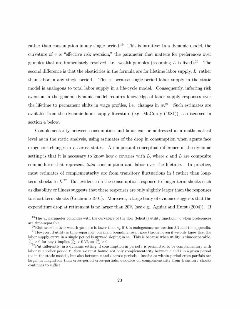
dollar. These choices are depicted by the intersections of the uc and ψwcurves in Figure 1.

Now consider the effect of an increase in w from w0 to w1 on compensated labor supply.

As shown in Figure 1, a change in w shifts the flat marginal disutility of labor curve down-

ward. If the utility function is highly curved (case A), the marginal utility of consumption

(uc) falls quickly as labor supply and income rise. Consequently, the increase in w leads

to a small increase in lcA. When the utility function is not very curved (case B), marginal

utility declines slowly as a function of wealth and the same ∆w leads to a larger increase

in lcB. Figure 1 therefore illustrates that the compensated wage (price) elasticity of labor

supply, εcl,w is inversely related to the curvature of utility over consumption.

The intuition for this relationship is as follows. Following a compensated wage increase,

agents increase their labor supply up to the point where the marginal utility of an additional

dollar is offset by the marginal disutility of the additional work necessary to earn that dollar.

If utility is very curved, this condition is met by a small increase in labor supply. If utility

is not very curved, the agent needs to increase l much more before his marginal utility of

money falls sufficiently to equal the new ψw1.

The preceding argument relies on the assumption that disutility of labor, ψ, does not vary

with l. When it does, the curvature of ψ(l) is confounded with the curvature of u and εcl,w is

no longer sufficient to recover γ. In this case, the elasticity of labor supply with respect to

unearned income, εl,y is needed to separate the two curvature parameters. Abstractly, the

8

l

u

ψ/w0

ψ/w1

Case B: γ low

Case A: γ high

∆lA ∆lB

∆w

uc(u-1(v+ψl))

Figure 1: Recovering γ from Labor Supply

income and compensated wage elasticities are both functions of the two curvatures. One can

therefore back out γ and the curvature of ψ by solving a system of two equations and two

unknowns, conditional on the degree of complementarity between consumption and leisure.

The next section derives the relationship between γ and labor supply elasticities formally

in the more general case where the marginal disutility of labor varies with l.

3.2 Base Case: Additive Utility

It is convenient to redefine u(c, l) as the agent’s utility over both consumption and labor.

Assume uc > 0, ul < 0, ucc < 0, ull < 0. In addition, assume utility is additive: ucl = 0.10

Consider an agent with wage w and unearned income y. Unearned income in this model

should not be thought of as only asset wealth. It also includes the income of the other earner

10Note that this restriction is stronger than assuming that the utility function permits an additivelyseparable representation. For example, Cobb-Douglas utility is “additively separable” but does not satisfythe additivity restriction (however, the log of a Cobb-Douglas utility does).

9

in dual-earner households and Hausman’s (1985) definition of “virtual income” to correct

for the non-linearity of the budget set created by the progressive tax system.11 This agent

chooses (Marshallian) labor supply l by solving

maxlu(y + wl, l)

At an interior optimum, l satisfies the first order condition

wuc(y + wl, l) = −ul(y + wl, l) (1)

Consider the effects of increasing w and y on l:

∂l

∂y= − wucc

w2ucc + ull∂l

∂w= − uc + wlucc

w2ucc + ull

Using the Slutsky decomposition for compensated labor supply (∂lc

∂w)

∂lc

∂w=

∂l

∂w− l ∂l

∂y(2)

it follows that∂l/∂y

∂lc/∂w=wucc(y + wl, l)

uc(y + wl, l)(3)

The definition of the coefficient of relative risk aversion at consumption c is

γ(c) ≡ −εuc,c =∂uc(c)

∂c

c

uc(c)= −ucc(c)

uc(c)c (4)

11Non-linear budget sets and dual earners could be explicitly introduced in the model, but these effectscan be handled more easily by changing the definition of y appropriately in the simple single-earner model.The empirical implementation in section 3 defines y appropriately to take these effects into account as in themodern labor supply literature.

10

which implies, using (3), that

γ(y + wl) = −y + wlw

∂l/∂y

∂lc/∂w= −(1 + wl

y)εl,yεlc,w

(y,w) (5)

where εl,y denotes the income elasticity, εlc,w the compensated wage (price) elasticity, andwlythe ratio of earned to unearned income.

As in the graphical example, the coefficient of relative risk aversion is inversely related

to the price elasticity. In addition, when disutility of labor is not constant, γ is directly

related to the magnitude of the income elasticity. To see why the ratio of these elasticities

determines risk aversion, recall that γ ∝ uccucwhere uc denotes the first derivative of utility

with respect to consumption, and ucc denotes the second derivative. An agent’s labor

supply response to a wage increase is directly related to uc: the larger the magnitude of uc,

the greater the benefit of an additional dollar of income, and the more the agent will work

when w goes up. The labor supply response to an increase in income is related to how

much the marginal utility of consumption changes as income changes, ucc. A large income

effect implies that the agent is willing to increase effort significantly in order to recoup lost

income, which means that the marginal utility of consumption rises quickly as income falls,

i.e. the magnitude of ucc is large. The connection between γ and the ratio of income and

price elasticities follows from these two observations.

The reader may be puzzled that we can identify a unique value for γ by observing only

labor supply. Since non-linear monotonic transformations of u(c, l) do not affect the choice

of l, are there not infinitely many values of γ that could be associated with observed labor

supply behavior? While this is true in general, the key is to observe that any non-linear

transformation of u will change the value of ucl. However, (5) was derived under the

assumption that u(c, l) is additive, i.e. ucl = 0.

It should be reiterated that γ is the curvature of utility over consumption.12 This

12This is the parameter estimated by most studies of choice under uncertainty, insofar as labor supply

11

coincides with the curvature of utility over wealth — the parameter that determines risk

preferences in an expected utility model — when labor supply is fixed. When labor supply

is variable, the curvature of utility over wealth is lower than γ. To see this, define indirect

utility over unearned income, which is equivalent to wealth in the static model, as

v(y) = u(y + wl(y), l(y))

It is shown in the appendix that the curvature of utility over unearned income is

−vyyvyy = γ

y + wlεl,yy + wl

< γ

Hence, our bound on γ effectively serves as a bound on curvature over wealth as well when

l is endogenous. Intuitively, when there are more margins over which an agent can adjust

expenditure, the curvature of utility over wealth falls because the marginal dollar can be

allocated more efficiently.

It is worth noting that frictions which prevent agents from reoptimizing fully in response

to perturbations in w and y will not affect our inferences about γ. For example, Status-quo

biases or institutional constraints that make small adjustments in labor supply difficult do

not affect the estimate. This is because the method is biased only by factors that affect the

price and income elasticities differently.13

The preceding derivation hinges on the assumption that utility is additive (ucl = 0). The

next section relaxes this assumption.

is omitted from these analyses. More importantly, it is the relevant parameter for many analyses of riskybehavior where shocks to labor supply are exogenous (e.g. optimal unemployment insurance).13To see this formally, note that an adjustment cost or status quo bias can be modeled as a cost k(l, l0) of

changing labor supply to l from l0. Since we make no assumptions about the way in which labor supply lenters u(c, l), (5) still obtains. The reason is that curvature is identified from the ratio of income and priceeffects, and k > 0 attenuates both effects.

12

3.3 Complementarity Between Labor and Consumption

When ucl 6= 0, (3) becomes∂l/∂y

∂lc/∂w= wucc/uc + ucl/uc (6)

which, after some rearrangement, implies that

γ(y + wl) = (1 +wl

y)−εl,yεlc,w

+ (1 +y

wl)εuc,l (7)

where εuc,l denotes the elasticity of the marginal utility of consumption with respect to labor

supply. Note that labor supply data is sufficient to identify γ given any value of εuc,l because

no non-linear transformation of u will leave εuc,l unchanged; in other words, εuc,l pins down

the cardinal normalization of the Bernoulli utility function.

It remains to estimate εuc,l. Since it is a cardinal concept, this parameter must be esti-

mated from choices under uncertainty. The most obvious method of estimating εuc,l, which

has been implemented in a set of empirical studies, is to exploit data on the consumption

choices of individuals who anticipate exogenous shocks to labor supply. For example, if an

agent plans to keep consumption fairly constant across states in which he is employed and

unemployed, εuc,l must be small.

To derive the relationship between consumption choices when employment is stochastic

and εuc,l formally, consider a world with two states. Agents supply l1 units of labor in state

1 and l2 units of labor in state 2. Suppose that the agent can trade consumption fairly

between the two states by purchasing state-contingent commodities (e.g. using an insurance

policy). He chooses consumption in the two states by maximizing expected utility

maxc1,c2

pu(c1, l1) + (1− p)u(c2, l2)s.t. pc1 + (1− p)c2 = pwl1 + (1− p)wl2 ≡W

The agent’s first-order condition for consumption is obtained by equating marginal utilities

13

across the two states:

uc(c1, l1) = uc(W − c1, l2)

Now, suppose we observe data from the following experiment. Assume that the agent

starts out supplying a constant l1 = l2 = l units of labor in each state. Suppose there is

a balanced-budget change in labor supply, increasing state 1 labor supply by δ1 units while

decreasing state 2 labor supply by δ2 units to keep expected earnings fixed at W . We

can think of this as a decision to increase work effort in state 1 to compensate for (partial)

unemployment in state 2.

Differentiating the first order condition with respect to l1 while holdings earnings fixed

at W yields the following identity:

εuc,l = γεc1,l1

Here, εc1,l1 denotes the elasticity of consumption with respect to labor supply in state 1

(while labor supply in state 2 changes so that total income remains constant). Plugging

this expression into (7) and solving gives an estimator for risk aversion in terms of εc1,l1 :

γ = (1 +wl

y)−εl,yεlc,w

/(1− (1 + y

wl)εc1,l1) (8)

This formula reduces to (5) when utility is additive in labor and consumption (εc1,l1 = 0).

When consumption and labor are complements, εc1,l1 > 0, and the true γ is higher relative

to the estimate obtained when additive utility over c and l is assumed.14 Hence, deriving

an upper bound on γ requires an upper bound on the value of εc1,l1 .

To obtain a bound on εc1,l1 , it is helpful to derive a connection between εc1,l1 and the con-

sumption drop during (full) unemployment that has been estimated in consumption studies.

14The sign of εc1,l1 is theoretically ambiguous. If consumption requires time, as in Becker (1965), leisureand consumption are complements (εc1,l1 < 0). On the other hand, work-related expenses can make laborand consumption complementary (εc1,l1 > 0). I show below that regardless of the sign of εc1,l1 , the estimatesof γ are not very sensitive to its magnitude.

14

Normalize the agent’s labor supply to 1 when working and 0 when unemployed. Since we

are using a discrete change in labor supply to infer an elasticity at a specific (c, l) pair, we

must choose a functional form for consumption in terms of labor supply. For simplicity, I

assume a linear form:

c = a+ bl

In this case, εc1,l1(l1 = 1) =ba+b, which is precisely the percentage drop in consumption from

the employed to unemployed state. Note that estimates of the consumption drop during

unemployment give an upper bound for the true εc1,l1 if agents cannot smooth consumption

across states to their desired level because of the inadequacy of available insurance policies,

lack of savings, or credit constraints (i.e., incomplete markets). Put differently, unemployed

agents are always free to consume less than they actually do when unemployed; it is only

consuming more that may be impossible because of liquidity constraints. Hence, their

actual consumption choices should, if anything, overstate the true degree of complementarity

between c and l.

Most estimates of the consumption drop are quite small. In a recent study of unemploy-

ment in the US, Gruber (1997) estimates ba+b

= 0.068 using data on food consumption from

the PSID. Gruber (1998) obtains estimates of similar magnitudes when examining data for

a broad set of consumption goods from the CEX.15 Browning, Hansen, and Heckman [BHH]

(1999) survey a number of other studies that estimate the consumption drop associated with

an exogenous labor supply change. Several studies estimate that c and l are actually sub-

stitutes (εc1,l1 < 0). The largest estimate of complementarity cited by BHH is a 30% drop

in consumption during unemployment. In view of this evidence, a plausible upper bound

for εc1,l1 is around 20% and an extreme value appears to be 30%. We will see in section 4

below that even this extreme value of εc1,l1 has little effect on our bound for γ. The bound

15Similarly, Browning and Crossley (2001) use data from the Canadian Out of Employment Panel to showthat the consumption drop is not statistically distinguishable from zero for households that have positiveliquid assets before their unemployment spell.

15

on risk aversion implied by labor supply behavior is thus insensitive to assumptions about

the degree of complementarity between consumption and labor, which is fortunate given the

lack of consensus in the literature about this parameter.

3.4 Extensive Labor Supply Decisions

Until this point, we have made the assumption that agents are able to freely choose the

number of hours they work. However, spikes in the hours distribution at 20 hours and 40

hours question the validity of this assumption. Many individuals appear to face the narrower

choice of either working for a fixed number of hours or not working at all.16 In this section,

I consider a model where hours choices are restricted and show that an estimator for risk

aversion can be derived using labor force participation data in this case.

To model extensive labor supply decisions, let us return to the static framework and

assume that the agent makes a binary decision to work and supply 1 unit of labor or not

work. As above, let y denote unearned income and w the income earned by working.

Returning temporarily to additive utility over consumption and leisure, redefine u(c) as the

utility from consumption. Let ψ denote disutility of supplying 1 unit of labor. The agent

chooses labor supply by solving

maxl∈{0,1}

u(y + wl)− ψl

He works if his disutility of labor is less than the utility of an additional w units of consump-

tion, i.e. if

ψ < bψ(y,w) ≡ u(y + w)− u(y)16The purpose of this section is to show that inferences about curvature can be made even when changes

in labor supply are lumpy. The nature of the lumpiness itself (e.g. whether there are restrictions on hoursworked in a week or weeks worked in a year) is not important.

16

Let us model the heterogeneity of disutility of labor in the economy by a smooth density

f(ψ). Then the fraction of workers who participate in the labor force is

θ(y, w) =Z bψ(y,w)0

f(ψ)dψ (9)

It follows that

− ∂θ/∂y

∂θ/∂w=uc(y)− uc(y + w)

uc(y + w)(10)

This expression shows that the percent change in marginal utility of wealth from y to y+w

is equal to the ratio of the income and wage effects on labor supply. In the intensive labor

supply model, we could compute γ(c) at any level c without making any functional form

assumptions because we could observe how marginal utility changes for small changes in

income. In a world with extensive labor supply decisions, we observe only the change in

marginal utility between y and y + w. Consequently, we need to make a functional form

assumption for u(c) to translate the change in marginal utilities into a coefficient of relative

risk aversion. I assume CRRA utility:17

u(c) =c1−γ

1− γ

Under this assumption, (10) implies

− ∂θ/∂y

∂θ/∂w=y−γ − (y + w)−γ(y + w)−γ

Solving for γ yields

γ =log[1− εθ,y

εθ,w

w

y]

log[1 +w

y]

(11)

Finally, a model of unemployment analogous to that above can be used to derive an

17If γ(c) actually varies with c, this method yields the best constant-γ fit of the data, which can be looselyinterpreted as the average γ(c) in the region c ∈ [y, y + w].

17

estimator for γ when utility is not additive:

γ =log[1− εθ,y

εθ,w

w

y]

log[(1− ∆cc)(1 +

w

y)]

(12)

where ∆ccdenotes the consumption drop associated with unemployment.

This concludes the analysis of risk aversion and labor supply in the static labor-leisure

choice model. The next subsection extends the preceding results to a dynamic setting.

3.5 Dynamics: Distinguishing EIS and γ

The fact that we have derived an estimator for risk aversion in a static model suggests

that the estimator fundamentally restricts preferences over states (risk aversion) rather than

preferences over time (intertemporal substitution). Establishing this point formally requires

analysis of a dynamic model where the EIS and γ are independent parameters. This subsec-

tion considers a standard dynamic life-cycle model and shows that (5) estimates “effective

risk aversion” — the curvature of the value function over wealth — leaving the EIS unidentified.

Consider a T period life-cycle model, and let consumption in each period be denoted by ct

and labor supply by lt. Note that the restrictive assumption that consumption equals income

implicit in the static analysis is dropped in this model. Allow utility to be completely non-

separable over time, leaving parameters governing intertemporal substitution unrestricted.18

Let wθt denote the wage in period t and y unearned income (period 0 wealth). In the

standard terminology of MaCurdy (1981), a change in θt is a transitory parametric wage

change, while changes in w are permanent wage changes, i.e. shifts in the entire profile of

wages. We will be interested in the latter effect: the relationship between l and w.

For simplicity, I first consider the case where utility is separable in c and l. Comple-

mentarity is addressed below. Exploiting separability, let u(c1, ..., cT ) denote utility over

18This preference structure nests commonly analyzed cases such as habit formation.

18

consumption and ψ(l1, ..., lT ) denote disutility over labor.

The agent solves

maxct,lt

u(c1, ..., cT )− ψ(l1, ..., lT )

s.t. c1 + ...+ cT = y + w(θ1l1 + ...+ θT lT )

This problem can be re-written as a two-stage maximization problem as follows:

maxc,L

v(c)−Ψ(L) s.t. c = y + wL (13)

where v(c) = maxct

u(c1, ..., cT ) | c1 + ...+ cT = cand Ψ(L) = min

ltψ(l1, ..., lT ) | θ1l1 + ...+ θT lT = L

Here, c is the composite commodity that represents total consumption, L is the composite

commodity that represents total labor, v is indirect utility over the composite consumption

good, and Ψ is indirect disutility over composite labor. Re-writing the problem in this

way is essentially an application of the composite commodity theorem. Note that since

the problem can be re-written in terms of indirect utilities even if the consumption path is

uncertain, introducing shocks into this model will not affect the results below.

The agent’s utility maximization problem over c and L in (13) has precisely the same

form as the static labor-leisure utility maximization problem given in section 3.2. The

derivation there thus yields an expression for the curvature of v:

γv ≡−vccvcc = −(1 + wL

y)εL,yεLc,w

(y,w) (14)

This formula is the same as that in (5), with two exceptions. First, the risk aversion

parameter γv is the curvature over indirect utility over the composite consumption good c,

19

rather than consumption in any single period.19 This is intuitive: In a dynamic model, the

curvature of v is “effective risk aversion,” the parameter that matters for preferences over

gambles that are immediately resolved, i.e. wealth gambles (assuming L is fixed).20 The

second difference is that the elasticities in the formula are for lifetime labor supply, L, rather

than labor in any single period. This is because single-period labor supply in the static

model is analogous to total labor supply in a life-cycle model. Consequently, inferring risk

aversion in the general dynamic model requires knowledge of labor supply responses over

the lifetime to permanent shifts in wage profiles, i.e. changes in w.21 Such estimates are

available from the dynamic labor supply literature (e.g. MaCurdy (1981)), as discussed in

section 4 below.

Complementarity between consumption and labor can be addressed at a mathematical

level as in the static analysis, using estimates of the drop in consumption when agents face

exogenous changes in L across states. An important conceptual difference in the dynamic

setting is that it is necessary to know how c covaries with L, where c and L are composite

commodities that represent total consumption and labor over the lifetime. In practice,

most estimates of complementarity are from transitory fluctuations in l rather than long-

term shocks to L.22 But evidence on the consumption response to longer-term shocks such

as disability or illness suggests that these responses are only slightly larger than the responses

to short-term shocks (Cochrane 1991). Moreover, a large body of evidence suggests that the

expenditure drop at retirement is no larger than 20% (see e.g., Aguiar and Hurst (2004)). If

19The γv parameter coincides with the curvature of the flow (felicity) utility function, γ, when preferencesare time-separable.20Risk aversion over wealth gambles is lower than γv if L is endogenous: see section 3.2 and the appendix.21However, if utility is time-separable, our main bounding result goes through even if we only know that the

labor supply curve in a single period is upward sloping in w. This is because when utility is time-separable,∂lt∂w > 0 for any t implies

∂lt∂w > 0 ∀t, so ∂L

∂w > 0.22Put differently, in a dynamic setting, if consumption in period t is perimitted to be complementary with

labor in another period t0, then we must bound not only complementarity between c and l in a given period(as in the static model), but also between c and l across periods. Insofar as within-period cross-partials arelarger in magnitude than cross-period cross-partials, evidence on complementarity from transitory shockscontinues to suffice.

20

one interprets this drop as an upper bound on complementarity between c and L, it would

be consistent with our bound on εc1,l1 in the static case. Hence, despite limited direct

evidence on what happens to c when there is a shock to L, it is difficult to imagine that

complementarity between consumption and labor in the long run is significantly larger than

the bounds placed on this parameter in section 3.3.

An important corollary of the preceding analysis is that the intertemporal elasticity of

substitution remains unrestricted while effective risk aversion is pinned down by labor supply

behavior when utility is time non-separable. It may be helpful to emphasize this point

by considering Kreps-Porteus utility, another commonly used method of severing the link

between EIS and risk aversion.23 Note that the Kreps-Porteus recursive utility specification

is simply a special case of the general time non-separable class of utility functions analyzed

above when agents are solving a labor-leisure choice problem without uncertainty. The

comparative statics of labor supply in the Kreps-Porteus model necessarily have the same

form as those in a general time non-separable model. An argument formally identical to

that given above for time non-separable utility therefore establishes that the estimator in

(5) yields the curvature of the value function over wealth for Kreps-Porteus utility. Hence,

our estimator identifies risk aversion over immediately-resolved (wealth) gambles for agents

with Kreps-Porteus utility as well.

The distinction between the EIS and γ clarifies the connection between this paper and the

work by King, Plosser and Rebelo (1988) and Basu and Kimball (2002) on labor supply and

intertemporal substitution discussed in section 2. Consider the case where utility is additive

over c and l. Here, the Basu and Kimball result is that time separability is inconsistent with

εl,w > 0 and low EIS. In contrast, this paper shows that state separability (i.e., expected

utility theory) is inconsistent with εl,w > 0 and high γ. The mathematics underlying these

two results is very similar, except that “time periods” have been relabeled as “states” in this

23The Kreps-Porteus specification is an expected-utility model for immediately resolved risks, and thereforefalls within the general framework analyzed in this paper.

21

paper. Conceptually, however, the results are quite different for two reasons. First, they

address two aspects of preferences — intertemporal substitution and risk aversion — which are

empirically and intuitively distinct from each other, as noted above. The result here places

no restrictions on the EIS; conversely, the results in KPR and Basu and Kimball place no

restrictions on risk aversion because they do not analyze a model with uncertainty. Second,

the solutions proposed by Basu and Kimball to resolve their “EIS puzzle” would not break

the link between risk aversion and labor supply behavior demonstrated here.

This concludes the theoretical portion of the paper. The next section implements the

formulas derived above using existing estimates of labor supply elasticities.

4 Empirical Implementation

4.1 A Calibration Argument

A large body of evidence points to a basic fact about labor supply: Individuals work more

when they get paid more to do so. An rich and diverse set of empirical studies of labor supply,

which are described in detail below, uniformly find that uncompensated labor supply curves

are weakly upward sloping (εl,w ≥ 0).24 The fact that εl,w ≥ 0 has strong implications

for risk aversion. To see this, first rewrite the Slutsky equation given in (2) in terms of

elasticities:

εlc,w = εl,w − lwyεl,y

Given εl,w ≥ 0, this formula yields a lower bound on εlc,w of − lwy εl,y. If ucl = 0, (5) canbe applied to obtain a bound on γ:

γ < 1 +y

wl

24This claim is further substantiated by a recent survey of 134 labor and public economists at 40 leadingresearch institutions by Fuchs, Krueger, and Poterba (1998). They found that the vast majority of theseexperts believe that the best estimate of the uncompensated wage elasticity is weakly positive.

22

The ratio of unearned income to earned income varies across the population, but in the

aggregate it equals the ratio of capital income to labor income, which is 12in the U.S. This

places an upper bound of γ = 1.5 for a representative agent whose utility is an income-

weighted average of individual utilities. Since capital income is highly concentrated, if we

are interested in the curvature of an equally-weighted average of utilities, the relevant value

of ywlis much lower; a reasonable estimate is 1

4.25 In this case, εl,w > 0 implies γ < 1.25 for

the representative agent when utility is additive in c and l. This bound also applies to the

curvature of the value function in dynamic models based on preceding arguments.

When additivity is relaxed, the upper bound becomes

γ < (1 +y

wl)/(1− (1 + y

wl)εc1,l1) (15)

As shown in section 3.3, a fairly loose upper bound for εc1,l1 is 0.2, which implies that

γ < 1.25/(1−0.25) = 1.66. Even in the extreme-case scenario of a 30% drop in consumptionassociated with unemployment — a value that Browning, Hansen, and Heckman (1999) argue

is an upward-biased estimate of the true degree of complementarity between c and l — the

estimate of γ rises to only 2. Hence, with relatively modest assumptions on complementarity

between c and l, the fact that the uncompensated labor supply curve is upward sloping

requires that risk aversion must be quite low in an expected utility model.

4.2 Imputing γ from Labor Supply Elasticities

This subsection gives a more complete picture of the values of γ implied by studies of labor

supply that estimate income and price elasticities. The traditional labor supply literature,

summarized by Pencavel (1986) and Blundell and MaCurdy (1999), defines “labor supply”

as hours worked or work participation. These studies estimate labor supply responses to

25Tabulations by the US Census Bureau (1999, Table E) adjusted for the progressivity of the income taxindicate that y

wl ≈ 14 for the median family in the U.S., which has an income of approximately $40,000.

23

permanent changes in wages and unearned income using variation such as tax changes, cross-

sectional differences, or lottery winnings.26 This literature can be broken into two strands.

The “static” or “reduced-form” literature estimates wage and income elasticities that yield

the relevant parameters for a static labor-leisure choice model. These studies employ cross-

sectional variation or changes in tax rates as a means of creating permanent, unanticipated

variations in budget sets. The credibility of static estimates has been questioned on the

grounds that cross-sectional variation introduces significant omitted variable bias and indi-

viduals are forward-looking in practice, which calls for formal modelling of the dynamics

involved. The “life cycle” or “structural” literature, pioneered by MaCurdy (1981) and

others, addresses this problem by explicitly modelling dynamic labor supply and consump-

tion choices and estimating labor supply responses to permanent shifts in wage profiles and

unearned income. I consider studies from both strands of the literature and show that the

implications for risk aversion are generally quite similar.

A more recent literature on labor supply, starting with Feldstein (1995), emphasizes that

hours worked is only one component of labor supply and that other margins such as effort

or training might adjust as well. When a multi-dimensional definition of labor supply is

incorporated into the models analyzed above, (5) still obtains except that the elasticity ratioεl,yεlc,w

is replaced by εLI,yεLIc,1−τ

, where LI is labor income and 1 − τ the net-of-tax rate. This

result follows the lines of Feldstein (1999), who shows that the elasticity of taxable labor

income with respect to the net-of-tax rate captures all margins on which taxable income can

be adjusted. The reason is that the relative prices of each mechanism of adjustment remain

fixed when tax rates change. Hence, recent estimates of the response of earned income to

changes in unearned income and tax rates can also be used to make inferences about γ.

Table 1 presents a set of income and wage elasticities for three definitions of labor supply:

26These studies estimate labor supply elasticities for a group of individuals, which might raise concernsabout aggregation if there is unobserved heterogeneity in risk preferences across agents. However, it can beproved that the estimator for γ derived in the representative agent model remains meaningful in this case;in particular, it yields a weighted average of risk aversion in the group.

24

(A) Hours worked, (B) Participation, and (C) Earned income.27 To get a sense of the plau-

sible range for γ that is consistent with labor supply behavior, I include elasticity estimates

for a wide range of groups, such as prime age males, married women, retired individuals, and

low income families. The inclusion of a diverse set of studies yields a substantial amount

of variation in the elasticities, ranging from 0.035 to 1.0 for the compensated wage elasticity

and —0.3 to -0.008 for the income elasticity. In general, elasticity estimates for groups who

are not as attached to the labor force (married women and older individuals) tend to be

higher than the elasticity estimates for groups with greater labor force attachment (prime

age males).

Column (6) of Table 1 reports estimates of γ at the average value of ywand l in each

study under the additive utility assumption. Note that the mean values of ywlvary widely

across the studies — e.g., married women’s unearned income equals at least their husband’s

income, which is generally larger than their own earned income. These variations are taken

into account in implementing (5). In addition, following Hausman (1985), y is defined as

“virtual” unearned income to account for the progressivity of the tax system.28

Strikingly, of the 29 sets of estimates used to construct this table, only one study implies

a value of γ above our calibration bound of 1.25 under the ucl = 0 assumption.29 The overall

(unweighted) mean estimate of γ across the twenty-nine studies is γ = 0.94, implying that

a 10% increase in consumption reduces the marginal utility of consumption by 9.4%. This

similarity of the estimates of γ despite the use of different methodologies, definitions of labor

supply, and groups of the population may be surprising at first. But it is quite intuitive in

view of the calibration argument given above — nearly all the studies of labor supply find

27In part (C) of the table, it is important to distinguish between taxable labor income and total laborincome. In the calculation of γ, we are interested in changes in total earned income, irrespective of the formof compensation. The measure of income used in the studies reported in the table is adjusted gross income(AGI), and may not capture forms of compensation that are not reported on tax returns such as office perks.28Since the earned income estimates combine different studies, they are evaluated at y

wl =14 , which reflects

the median value of unearned to earned income in the US (see above).29The estimates reported for the Blundell and MaCurdy (1999) are an average of the estimates of 20

studies surveyed in their paper, all of which imply γ < 1.25.

25

εl,w ≥ 0, which we know places a tight upper bound on γ.30

Column (7) of Table 1 reports estimates of γ that account for the degree of complemen-

tarity implied by the upper-bound on the unemployment consumption drop computed in

section 3.3 (∆cc= 20%). This adjustment increases the average estimate of γ to 1.33. In

view of the calibration arguments, it should not be surprising that taking complementarity

between labor and consumption into account does not raise the estimates of γ significantly.

5 Conclusion

Empirical studies of labor supply uniformly find that the uncompensated wage elasticity

of labor supply is positive: Individuals work more (or at least not much less) when their

wages rise. This paper has shown that this fact reveals considerable information about the

rate at which the marginal utility of wealth diminishes, which determines risk aversion in

expected utility models. To be consistent with an upward-sloping labor supply curve, the

coefficient of relative risk aversion must be less than 1.25 in the case where consumption and

leisure are not complementary. This bound rises to at most 1.66 over the range of plausible

perturbations of complementarity between consumption and labor. In a dynamic life-cycle

model with a fully general time non-separable utility, effective risk aversion — the parameter

that determines risk preferences over wealth gambles — is bounded by the same values.

The most important message of this paper is that those who work in the canonical one-

good expected utility framework must be content with a relatively low level of risk aversion

in view of well-established facts about labor supply behavior. This means that either

true risk preferences cannot explained by a standard expected utility model or that risk

aversion is truly low. It should be noted, however, that many economists think that risk

aversion is high and that uncompensated wage elasticities are positive. For instance, in

30Pencavel (1986), Blundell and MaCurdy (1999), and Gruber and Saez (2000) summarize more than sixtyother studies with an array of methodologies, nearly all of which find εl,w ≥ 0 and therefore imply γ < 1.25as well.

26

recommending parameters for neoclassical macro models on the basis of micro-econometric

studies, Browning, Hansen, and Heckman (1999) state that (1) the uncompensated wage

elasticity of labor supply is (weakly) positive, (2) the elasticity of consumption with respect

to labor, holding wealth fixed, is at most 0.3 (i.e., the degree of complementarity between

consumption and labor is not extremely large), and (3) the best estimate of γ is around

4. These three recommendations are not mutually consistent with the canonical expected

utility theory of risk preferences.

How can high risk aversion be reconciled with an upward-sloping labor supply curve?

What is needed is a dimension to risk aversion beyond diminishing marginal utility. Several

existing non-expected utility theories that alter probability weights on outcomes have such

a dimension. Examples include Chew and MacCrimmon’s (1979) weighted expected utility,

Quiggin’s (1982) rank-dependent utility, and Tversky and Kahneman’s (1992) cumulative

prospect theory. Abstractly, these theories change an agent’s utility valuation of a lottery

x = (p1, x1; ...; pn, xn) fromPpiu(xi) to

Pg(pi)u(xi) where g is a weighting function that,

appropriately parametrized, can introduce an additional source of risk aversion into the

model.31 Testing the performance of such theories under the constraint that u has a low

degree of curvature could be a fruitful course for further research.

31See Starmer (2000) and references therein for a detailed review of these and other theories of riskpreferences.

27

References

Acemoglu, Daron and Robert Shimer, “Efficient Unemployment Insurance,” Journal ofPolitical Economy 107 (1999), 893-928.Aguiar, Mark and Erik Hurst, “Consumption vs. Expenditure,” NBER Working Paper

10307 (2004).Allais, Maurice, “Le Comportement de l’Homme Rationnel devant le Risque: Critique

des postulats et axiomes de l’École Americaine,” Econometrica (1953).Auten, Gerald and Robert Carroll, “The Effect of Income Taxes on Household Behavior,”

Review of Economics and Statistics, 81 (1999), 681-693.Barsky, Robert B., F. Thomas Juster, Miles S. Kimball, and Matthew D. Shapiro, “Pref-

erence Parameters and Behavioral Heterogeneity: An Experimental Approach in the Healthand Retirement Study,” Quarterly Journal of Economics, CXII (1997), 537-580.Basu, Susanto and Miles Kimball, “Long-Run Labor Supply and the Elasticity of In-

tertemporal Substitution for Consumption,” University of Michigan mimeo, 2002.Becker, Gary, “A Theory of the Allocation of Time,” Economic Journal, 75 (1965), 493-

517.Blundell, Richard and Thomas MaCurdy, “Labor Supply: A Review of Alternative Ap-

proaches,” in Ashenfelter, Orley and David Card, eds., Handbook of Labor Economics 3(Amsterdam: North-Holland, 1999).Bodie, Zvi and William Samuelson, “Labor Supply Flexibility and Portfolio Choice in a

Life Cycle Model”, Journal of Economic Dynamics and Control 16 (1992), 427-450.Browning, Martin and Timothy Crossley, “Unemployment Insurance Benefit Levels and

Consumption Changes,” Journal of Public Economics, 80 (2001), 1-23.Browning, Martin, Lars Peter Hansen and James Heckman, “Micro Data and General

Equilibrium Models”, Handbook of Macroeconomics, Volume 1A, edited by John Taylor andMichael Woodford, North Holland, Amsterdam (1999).Chew, S.H. and K.R. MacCrimmon “Alpha-nu Choice Theory: A generalization of ex-

pected utility theory”, Working Paper No. 669, University of British Columbia, Vancouver(1979).Cochrane, John H, “A Simple Test of Consumption Insurance.” Journal of Political

Economy 99 (1991), 957-76.Dreze, Jacques, Essays on Economic Decisions Under Uncertainty (Cambridge: Cam-

bridge Univ. Press, 1987).Eissa, Nada and Hoynes, Hillary, “The Earned Income Tax Credit and the Labor Supply

of Married Couples,” NBER Working Paper 6856 (1998).Epstein, L. G., “Behavior Under Risk: Recent Developments in Theory and Applica-

tions,“ in Advances in Economic Theory, vol. II, edited by Jean-Jacques Laffont, CambridgeUniversity Press, 1-63 (1992).

28

Epstein, Larry and Stanley Zin, “Substitution, Risk Aversion, and the Temporal Behaviorof Consumption and Asset Returns: An Empirical Analysis,” Journal of Political Economy99 (1991), 263-286.Feldstein, Martin, “The Effect of Marginal Tax Rates on Taxable Income: A Panel Study

of the 1986 Tax Reform Act,” Journal of Political Economy, 103 (1995), 551-572.Feldstein, Martin, “Tax Avoidance and the Deadweight Loss of the Income Tax,” Review

of Economics and Statistics, 81 (1999), 674-680.Friedberg, Leoria, “The Labor Supply Effects of the Social Security Earnings Test,”

Review of Economics and Statistics, 82 (2000), 48-63.Fuchs, Victor, Alan B. Krueger and James M. Poterba, “Economists’ Views about Pa-

rameters, Values, and Policies: Survey Results in Labor and Public Economics,” Journal ofEconomic Literature 36 (1998), 1387-1425.Gruber, Jonathan, “The Consumption Smoothing Benefits of Unemployment Insurance,”

American Economic Review, 87 (1997), 192-205.Gruber, Jonathan, “Unemployment Insurance, Consumption Smoothing, and Private

Insurance: Evidence from the PSID and CEX,” Research in Employment Policy 1 (1998),3-31.Gruber, Jonathan and Emmanuel Saez, “The Elasticity of Taxable Income: Evidence and

Implications,” NBER Working Paper 7512 (2000).Hall, Robert, “Intertemporal Substitution in Consumption,” Journal of Political Econ-

omy 96 (1988), 339-357.Haubrich, Joseph G. “Risk Aversion, Performance Pay, and the Principal-Agent Problem,

” The Journal of Political Economy 102 (1994), 258-276.Hausman, Jerry, “Taxes and Labor Supply,” in Feldstein, Martin and Alan Auerbach,

eds., Handbook of Public Economics 1 (Amsterdam: North Holland, 1985).Imbens, Guido, Donald B. Rubin, and Bruce I. Sacerdote, “Estimating the Effect of

Unearned Income on Labor Earnings, Savings, and Consumption: Evidence from a Surveyof Lottery Players,” American Economic Review, 91 (2001), 778-794.Kaplow, Louis, “The Value of a Statistical Life and the Coefficient of Relative Risk

Aversion,” NBER Working Paper No. 9852 (2003).King, Robert, Charles Plosser, and Sergio Rebelo,“Production, Growth and Business

Cycles I. The Basic Neoclassical Model,” Journal of Monetary Economics 21 (1988) 309-341.Kocherlakota, Narayana, “The Equity Premium: It’s Still a Puzzle,” Journal of Economic

Literature, 24 (1996), 42-71.MaCurdy, Thomas, “An Empirical Model of Labor Supply in a Life-Cycle Setting,” The

Journal of Political Economy 89 (1981), 1059-1085.MaCurdy, Thomas, David Green, and Harry Paarsh, “Assessing Empirical Approaches

for Analyzing Taxes and Labor Supply,” Journal of Human Resources, 25 (1990), 415-90.Mehra, Rajnish and Edward C. Prescott, “The Equity Premium: A Puzzle,” Journal of

Monetary Economics, 15 (1985), 145-161.

29

Metrick, Andrew, “A Natural Experiment in Jeopardy!,” American Economic Review,85 (1995), 240-253.Palacios-Huerta, Ignacio, Roberto Serrano, and Oscar Volij, “Rejecting Small Gambles

Under Expected Utility,” Brown Univ. mimeo (2004).Pencavel, John, “Labor Supply of Men: A Survey” in Ashenfelter, Orley and Richard

Layard, eds, Handbook of Labor Economics 1 (Amsterdam: North Holland, 1986).Quiggin, John, ‘A theory of anticipated utility’, Journal of Economic Behavior and Or-

ganization 3 (1982), 323—43.Rabin, Matthew, “Risk Aversion and Expected-Utility Theory: A Calibration Theorem,”

Econometrica, 68 (2000), 1281-1292.Segal, U. and A. Spivak, “First Order Versus Second Order Risk Aversion,” Journal of

Economic Theory 51 (1990), 111-125.Starmer, C. (2000). Developments in non-expected utility theory: The hunt for a de-

scriptive theory of choice under risk. Journal of Economic Literature. 38, 332-382.Szpiro, George, “Measuring Risk Aversion: An Alternative Approach,” The Review of

Economics and Statistics, 68 (1986), 156-159.Tversky, Amos, & Daniel Kahneman, “Advances in prospect theory: Cumulative repre-

sentation of uncertainty.” Journal of Risk and Uncertainty, 5 (1992), 297-323.U.S. Census Bureau, Current Population Reports P60-209. Money Income in the United

States (1999).Weil, P. “Non-Expected Utility in Macroeconomics,” Quarterly Journal of Economics

29—42 (1990).

Kahneman, Daniel, Peter P. Wakker, and Rakesh Sarin, “Back to Bentham? Explo-rations of Experienced Utility,” Quarterly Journal of Economics, CXII (1997), 375-405.Kandel, Shmuel and Robert F. Stambaugh, “Asset Returns and Intertemporal Prefer-

ences,” Journal of Monetary Econmics, 27 (1991), 39-71.Machina, Mark, “Choice Under Uncertainty: Problems Solved and Unsolved,” Journal

of Economic Perspectives, 1 (1987), 121-154.Prelec, Drazen, “The Probability Weighting Function,” Econometrica, 66 (1998), 497-

527.Tversky, Amos and Craig Fox, “Weighting Risk and Uncertainty,” Psychological Review,

102 (1994), 269-283.Wu, George and Richard Gonzalez, “Curvature of the Probability Weighting Function,”

Management Science, 42 (1996), 1676-1690.

30

Appendix: Curvature of utility over unearned income

The Envelope theorem implies that

vy(y) = uc(c(y), l(y))

and it follows that

γy = −vyyvyy = −ucc

uc

∂c

∂yy

Recognizing that ∂c/∂y = 1 + w∂l/∂y, we obtain

γy = γεc,y

where εc,y denotes the income elasticity of consumption. Finally, observe that

εc,y =y + wlεl,yy + wl

where εl,y is the income elasticity of labor supply. Since εc,y < 1, it follows that γy < γ.

31

TABLE 1 Labor Supply Elasticities and Implied Coefficients of Relative Risk Aversion

Income Compensated γ γStudy Sample Identification Elasticity Wage Elasticitya Additive ∆c/c=0.2

(1) (2) (3) (4) (5) (6) (7)

A. Hours

MaCurdy (1983) Married Men Panel -0.020 0.130 0.77 1.03Blundell and MaCurdy (1999)b Men Various -0.120 0.567 1.06 1.41MaCurdy et al (1990) Married Men Cross Section -0.010 0.035 1.47 1.96Eissa and Hoynes (1998) Married Men, Inc < 30K EITC Expansions -0.030 0.192 0.88 1.17

Married Women, Inc < 30K EITC Expansions -0.040 0.088 0.64 2.12Friedberg (2000) Older Men (63-71) Soc. Sec. Earnings Test -0.297 0.545 0.93 1.80Average 1.03 1.45

B. Participation c

Eissa and Hoynes (1998) Married Men, Inc < 30K EITC Expansions -0.008 0.033 0.44 0.50Married Women, Inc < 30K EITC Expansions -0.038 0.288 0.15 0.45

Average 0.29 0.48

C. Earned Income d

Imbens et al (2001) Lottery Players in MA Lottery Winnings -0.110Feldstein (1995) Married, Inc > 30K TRA 1986 1.040 0.53 0.71Auten and Carroll (1997) Single and Married, Inc>15K TRA 1986 0.660 0.83 1.11Average 0.45 0.61Overall Average 0.94 1.33 aIn part (C), this column gives the elasticity of earned income with respect to the net-of-tax rate bThis row uses an unweighted average of the 20 elasticities reported in Blundell and MaCurdy (1999) and assumes y/wl=1/4 cParticipation elasticities assume CRRA utility dSince studies on earned income do not estimate income elasticties, I use the Imbens et. al. estimate in each case

32