Embed Size (px)
DESCRIPTION
Libro sobre teoría de la dinámica discreta. Y muchas más aplicaciones. No se recomienda en caso de niveles de ingeniería, pues se tiene un nivel mucho más avanzado.
Citation preview


DIFFERENCE EQUATIONS WITH APPLICATIONS TO QUEUES
. .. . . , ".,,*. .. . . . , . X ...... ~ ,.".. .I, .. I . I. .. ..-., .X.I. .., ...I. . ".. , , . . . . ... .. . . .- . ...... .... . _ ., . , , I.

PURE AND APPLIED MATHEMATICS
A Program of Monographs, Textbooks, and Lecture Notes
EXECUTIVE EDITORS
Earl J. Taft Rutgers University
New Brunswick, New Jersey
Zuhair Nashed University of Delaware
Newark, Delaware
EDITORIAL BOARD
M. S. Baouendi Ani1 Nerode University of California, Cornel1 University
San Diego Donald Passman
Jane Cronin University of Wisconsin, Rutgers University Madison
Jack K. Hale Fred S. Roberts Georgia Institute of Technology Rutgers University
S. Kobayashi David L. Russell University of California, Virginia Polytechnic Institute
Berkeley and State University
Marvin Marcus Walter Schempp
Santa Barbara University of California, Universitat Siegen
Mark Teply
Yale University Milwaukee W. S. Massey University of Wisconsin,
MONOGRAPHS AND TEXTBOOKS IN PURE AND APPLIED MATHEMATICS
1. K. Yano, Integral Formulas in Riemannian Geometry (1970) 2. S. Kobayashi, Hyperbolic Manifolds and Holomorphlc Mappings (1 970) 3. V. S. Vladimimv, Equations of Mathernatlcal Physics (A. Jeffrey, ed.; A. Littlewood,
4.
5. 6. 7.
8. 9.
IO. 11.
trans.) (1 970) B. N. Pshenichnyi, Necessary Conditions for an Extremum (L. Neustadt, translation ed.; K. Makowski, trans.) (1971) L. Nariciet al., Functional Analysis and Valuatlon Theory (1971) S. S. Passman, Infinite Group Rings (1971) L. Domhoff, Group Representation Theory. Part A Ordinary Representation Theory. Part B: Modular Representation Theory (1971, 1972) W. Boothbv and G. L. Weiss, eds.. Svmmetric %aces (1972) Y. Matsushima, Differentiable Manifoids (E. T. Kobayashi, trans.) (1972) L. E. Ward, Jr., Topology (1972) A. Babakhanian. Cohomoloaical Methods in GrouD Theorv (19721
12. R. Gilmer, Multiplicative Ideal Theory (1972) 13. J. Yeh, Stochastic Processes and the Wiener Integral (1973) 14. J. Barns-Neto, Introduction to the Theory of Distributlons (1973) 15. R. Larsen, Functional Analysis (1 973) 16. K. Yano and S. Ishiham, Tangent and Cotangent Bundles (1 973) 17. C. Pmcesi, Rings with Polynomial Identities (1 973) 18. R. Hennann, Geometry, Physics, and Systems (1973)
20. J. Dieudonnd, Introduction to the Theory of Formal Groups (1973) 19. N. R. Wallach, Harmonic Analysis on Homogeneous Spaces (1 973)
21. l. Vaisman, Cohomology and Differential Forms (1973) 22. B.-Y. Chen, Geometry of Submanifolds (1973) 23. M. Marcus, Finite Dimensional Multilinear Algebra (in two parts) (1973, 1975) 24. R. Larsen, Banach Algebras (1973) 25. R. 0. Kujala and A. L. Viffer, eds., Value Distribution Theory: Part A; Part B: Deficit
26. K. B. Stolarsky, Algebraic Numbers and Diophantine Approximation (1974) 27. A. R. Magid, The Separable Galois Theory of Commutative Rings (1974) 28. B. R. McDonald, Finite Rings with Identity (1974) 29. J. Satake, Linear Algebra (S. Koh et al., trans.) (1975) 30. J. S. Golan, Localization of Noncommutative Rings (1975) 31, G. Klambauer, Mathematical Analysis (1 975) 32. M. K. Agoston, Algebraic Topology (1976) 33. K. R. Goodearl, Ring Theory (1976) 34. L. E. Mansfield, Linear Algebra with Geometric Applications (1 976) 35. N. J. Pullman, Matrix Theory and Its Applications (1976) 36. B. R. McDonald, Geometric Algebra Over Local Rings (1 976) 37. C. W. Gmetsch, Generalized Inverses of Linear Operators (1977) 38. J. E. Kuczkowski and J. L. Gersting, Abstract Algebra (1 977) 39. C. 0. Christenson and W. L. Voxman, Aspects of Topology (1977) 40. M. Nagafa, Field Theory (1977) 41, R. L. Long, Algebraic Number Theory (1977) 42. W. F. Pfeffef, Integrals and Measures (1977) 43. R. L. Wheeden and A. Zygmund, Measure and integral (1977)
45. K. Hrbacek and T. Jech, Introduction to Set Theory (1978) 44. J. H. Curtiss, Introduction to Functions of a Complex Variable (1978)
46. W. S. Massey, Homology and Cohomology Theory (1 978) 47. M. Marcus, introduction to Modern Algebra (1978) 48. E. C. Young, Vector and Tensor Analysis (1 978) 49. S. B. Nadler, Jr., Hyperspaces of Sets (1978) 50. S. K. Segal, Topics in Group Kings (1978) 51. A. C. M. van RooJ, Non-Archimedean Functional Analysis (1978) 52. L. Corwin and R. Szczafba, Calculus in Vector Spaces (1979) 53. C. Sadosky, Interpolation of Operators and Singular Integrals (1979) 54. J. Cmnin, Differentlal Equations (1980) 55. C. W. Gmetsch, Elements of Applicable Functional Analysis (1980)
_ . .
and Bezout Estimates by Wllhelm Stoll(1973)

56. 57. 58. 59. 60. 61. 62.
63. 64. 65. 66. 67. 68.
. ..
69. 70. 71. 72. 73. 74. 75. 76. 77. 78. 79. 80. 81. 82. 83.
84. 85. 86. 87. 88. 89. 90.
91. 92. 93. 94. 95. 96. 97 I 98.
99. 100. 101. 102. 103.
104. 105. 106.
107. 108. 109. 110.
111. 112.
l. Vaisman, Foundations of Three-Dimensional Euclidean Geometry (1980) H. l. Freedan, Deterministic Mathematical Models In Population Ecology (1 980) S, B. Chae, Lebesgue Integration (1980)
L. Nachbin, Introduction to Functional Analysis (R. M. Aron, trans.) (1981) C. S. Rees et el,, Theory and Applications of Fourier Analysls (1 981)
R. Johnsonbaugh and W. E. Pfafenberger, Foundations of Mathematical Analysis G, Omch and M. Onech, Plane Algebraic Curves (1 981)
(1981) W, L. Voxman and R. H. Goetschel, Advanced Calculus (1981) L. J. Cowin and R. H. Szczafba, Multivariable Calculus 1982) V. l. lstr#escu, Introduction to Linear Operator Theory (1 B 81) R. D. J&vinen, Flnite and infinite Dimensional Linear Spaces (1981) J. K. Beem andf. E. Ehriich, Global Lorentzian Geometry (1981) D. L. Atmacost, The Structure of Locally Compact Abelian Groups (1981) J. W. Brewerand M. K, Smith, eds., Emmy Noether: A Tribute (1981) K. H. Kim, Boolean Matrix Theory and Applications (1982) T. W. Wieting, The Mathematical Theory of Chromatic Plane Ornaments (1982) D. B. Gauld, Differential Topology (1 982) R. L. Faber, Foundations of Euclidean and Non-Euclidean Geometry (1983) M. Cameli, Statistical Theory and Random Matrices (1983) J. H. Canuth et al., The Theory of Topological Semigroups (1983) R. L. Faber, Differential Geometry and Relativity Theory (1983) S. Bamett, Polynomials and Linear Control Systems (1983) G. Kapilovsky, Commutative Group Algebras (1983) F. Van Oystaeyen and A. Verschoren, Relative Invariants of Rings (1983) l. Vaisman, A First Course In Differential Geometry (1984) G. W. Swan, Applications of Optimal Control Theory in Blomediclne (1984) T. Petrie andJ. D. Randall, Transformation Groups on Manifolds (1984) K, Goebel and S. Reich, Unlform Convexity, Hyperbolic Geometry, and Nonexpansive Mappings (1 984) T. Albu and C. Ndst&escu, Relative Finiteness in Module Theory (1984) K. HnSacek and T. Jech, Introduction to Set Theory: Second Edition (1984) F. Van Oystaeyen andA. Verschoren, Relative Invariants of Rings (1984) B. R. McDonald, Linear Algebra Over Commutative Rings (1984) M. Namba, Geometry of Projective Algebraic Curves (1 984) G. F. Webb, Theory of Nonlinear Age-Dependent Population Dynamics (1985) M. R. Bmmner et al., Tables of Dominant Weight Multiplicities for Representations of Simple Lie Algebras (1 985) A. E. Fekete, Real Linear Algebra (1985) S. B. Chae, Holomorphy and Calculus in Normed Spaces (1 985) A. J. Jeni, Introduction to Integral Equations with Applications (1985) G. Kapilovsky, Projective Representations of Finite Groups (1985) L. Narici and E. Beckenstein, Topological Vector Spaces (1 985) J. Weeks, The Shape of Space (1985) P. R. Gribik and K. 0. Kortanek, Extrema1 Methods of Operations Research (1 985) &A. Chao and W. A. Woyczynski, eds., Probability Theory and Harmonic Analysis (1 986) G. D. Crown et al., Abstract Algebra (1 986) J. H. Canuth et al., The Theory of Topological Semigroups, Volume 2 (1986) R. S. Dofan and V. A. 6el17, Characterizations of C*-Algebras (1986) M. W. Jeter, Mathematical Programming (1986) M. Altmen, A Unified Theory of Nonlinear Operator and Evolution Equatlons with Applications (1 986) A. Verschoren, Relative Invariants of Sheaves (1987) R. A. Usmani, Applied Linear Algebra (1987) P. Blass and J. Lang, Zariski Sutfaces and Differential Equations in Characteristic p z 0 (l 987) J. A. Reneke et al., Structured Hereditary Systems (1987) H. Busemann and B. B. fhadke, Spaces with Distinguished Geodesics (1987) R. Ha&, Invertibility and Singularity for Bounded Linear Operators (1988)
ments (1 987) G. S. Ladde et al., Osclllation Theory of Differential Equations with Deviating Argu-
L. Dudkin et al., lteratlve Aggregation Theory (1987) T. Okubo, Differentlal Geometry (1 987)

11 3. D. L. Stancl and M. L. Stancl, Real Analysis with Point-Set Topology (1 987) 114. T. C. Gad, Introduction to Stochastic Differential Equations (1988) 115. S. S. Abhyankaf, Enumerative Combinatorics of Young Tableaux (1988) 116. H. Strade and R. Fernsteiner, Modular Lie Algebras and Their Representations (1988) 117. J. A. Huckaba, Commutative Rings with Zero Divisors (1988) 118. W D. Wdlis, Combinatorial Designs (1988) 1 19. W Wips/aw, Topological Flelds (1 988) 120. G. Karpilovsky, Field Theory (1 988) 121. S. Caenepeel and F. Van Oystaeyen, Brauer Groups and the Cohomology of Graded
122. W. Kozlowski, Modular Function Spaces (1988) 123. E. Lowen-Colebunders, Function Classes of Cauchy Continuous Maps (1989) 124. M. Pave/, Fundamentals of Pattern Recognition (1989) 125. V. Lakshmikanfham et al., Stability Analysis of Nonlinear Systems (1989) 126. R. Sivaramakrishnan, The Classical Theory of Arithmetic Functions (1989) 127. N. A. Watson, Parabolic Equations on an Infinite Strip (1989) 128. K. J. Hastings, Introduction to the Mathematlcs of Operations Research (1989) 129. 6. Fine, Algebraic Theory of the Bianchi Groups (1989) 130. D. N. Dikranjan et al., Topological Groups (1989) 131. J. C. Morgan /l, Point Set Theory (1990) 132. P. 8ilerandA. Wtkowski, Problems in Mathematical Analysis (1990) 133. H. J. Sussmann, Nonlinear Controllability and Optimal Control (1990) 134. &P. Flomns et al., Elements of Bayesian Statistics (1990) 135. N. Shell, Topological Fields and Near Valuations (1990) 136. 8. F. Doolin and C. F. Martin, Introduction to Differential Geometry for Engineers
137. S. S. Holland, Jr., Applied Analysls by the Hilbert Space Method (1 990) 138. J. Oknlnski, Semigroup Algebras (1 990) 139. K. Zhu, Operator Theory In Function Spaces (1 990) 140. G. 6. Price, An Introduction to Multicomplex Spaces and Functions (1991) 141. R. 6. Darst, Introduction to Linear Programming (1991) 142. P. L. Sachdev, Nonllnear Ordinary Differential Equations and Their Applications (1991) 143. T. Husain, OrVlogonal Schauder Bases (1991) 144. J. Foran, Fundamentals of Real Analysis (1991) 145. W. C. Brown, Matrices and Vector Spaces (1991) 146. M. M. Rao andZ. D. Ren, Theory of Oriicz Spaces (1991) 147. J. S. Golan and T. Head, Modules and the Structures of Rings (1991) 148. C. Small, Arithmetic of Finite Fields (1 991) 149. K. Yang, Complex Algebraic Geometry (1991) 150. D. G. Hofmanetal., CodingTheory(1991) 151, M. 0. Gonzdlez, Classical Complex Analysis (1992) 152. M. 0. Gonzdlez, Complex Analysis (1 992) 153. L. W. Baggett, Functional Analysis (1992) 154. M. Sniedovich, Dynamic Programming (1992) 155. R. P. Aganval, Difference Equations and Inequalities (1992) 156. C. Bmzinski, Biorthogonality and Its Applications to Numerical Analysis (1992) 157. C. Swartz, An lntroductlon to Functional Analysis (1992) 158. S. 6. Ned& Jr., Continuum Theory (1992) 159. M. A. ACGwaiz, Theory of Distributions (1992) 160. E. Perry, Geometry: Axiomatic Developments with Problem Solving (1992) 161. E. Castillo and M. R. Ruiz-Cobo, Functional Equations and Modelling in Science and
162. A. J. Jem', Integral and Discrete Transforms with Applications and Error Analysis
163. A. Chadieret al., Tensors and the Clifford Algebra (1992) 164. P, Mer and T. Nadzieja, Problems and Examples in Differential Equations (1 992) 165. E. Hansen, Global Optimization Uslng Interval Analysis (1992) 166. S. Guem-DelabriBm, Classical Sequences in Banach Spaces (1992) 167. Y. C. Wong, Introductory Theory of Topologlcal Vector Spaces (1992) 168. S. H. Kulkami and 6. V. Limaye, Real Function Algebras (1992) 169. W. C. Brown, Matrices Over Commutative Rings (1 993) 170. J. Loustau and M. Dillon, Linear Geometry with Computer Graphics (1993) 171. W. V. Petryshyn, Approximation-Solvability of Nonlinear Functional and Differential
Rings (1 989)
(1990)
Engineering (1992)
(1 992)
Equations (1993)

172. 173. 174. 175. 176. 177. 178.
179. 180.
181.
182.
184. 183.
185. 186. 187. 188.
189. 190. 191. 192.. 193. 194. 195. 196. 197.
198. 199. 200. 201. 202. 203. 204. 205. 206. 207. 208. 209. 21 0.
211. 212. 21 3. 214.
21 5. 216.
217. 218. 219.
220. 221.
223. 222.
224. 225.
E. C. Young, Vector and Tensor Analysis: Second Edition .( 1993)
M. Pavel, Fundamentals of Pattern Recognition: Second Edition (1993) T A. Bick, Elementary Boundary Value Problems (1993)
S. A. Albeverio eta/., Noncommutative Dlstributions (1993) W. Fulks, Complex Variables (1 993) M. M. Rao, Conditional Measures and Applications (1 993) A. Janicki and A. Wemn, Simulation and Chaotic Behavior of a8table Stochastic Processes (1 994) P. Neittaanmeki and D. Tiba, Optimal Control of Nonlinear Parabolic Systems (1994) J. Cmnin, Differential Equations: Introduction and Qualitative Theory, Second Edition (1994) S. Heikkild and V. Lakshrnikantharn, Monotone Iterative Techniques for Discontinuous Nonlinear Differential Equations (1994) X. Mao, Exponential Stability of Stochastic Dlfferential Equations (1994)
J. E. Rubio, Optimization and Nonstandard Analysis (1 994) 6. S. Thornson, Symmetric Properties of Real Functions (1 994)
J. L. 6ueso eta/., Compatibility, Stability, and Sheaves (1995) A. N. Michel and K. Wang, Qualitative Theory of Dynamical Systems (1995) M. R. Darnel, Theory of Lattice-Ordered Groups (1 995) 2. Naniewicz and P. D. Panagiotopoulos, Mathematical Theory of Hemivariationai
L. J. Corwin and R. H. Szczarba, Calcuius in Vector Spaces: Second Edition (1995) Inequalities and Applications (1995)
L. H. €he et al., Oscillation Theory for Functional Dlfferential Equations (1995) S. Agaian et ab, Binary Polynomial Transforms and Nonlinear Digital Filters (1995) .M. l. Gil: Norm Estimations for Operation-Valued Functions and Applications (1995) P. A. Grillet, Semigroups: An Introduction to the Structure Theory (1995) S. Kichenassamy, Nonlinear Wave Equations (1 996) V. F. Kmtov, Global Methods in Optimal Control Theory (1996) K. l. Beidaret ab, Rings with Generalized Identities (1996)
(1 996) V. l. Amautov et al., Introduction to the Theory of Topological Rings and Modules
G. Sierksrna, Linear and Integer Programming (1996) R. Lasser, Introduction to Fourier Series (1996) V. Sima, Algorithms for Linear-Quadratic Optimization (1996) D. Redrnond, Number Theory (1 996) J. K. 6eem et al., Global Lorentzian Geometry: Second Edition (1996) M. Fontana et al., Prllfer Domains (1 997) H. Tanabe, Functional Analytic Methods for Partial Differential Equations (1997)
E. Spiegeland C. J. O’Donnell, Incidence Algebras (1997) C. Q. Zhang, Integer Flows and Cycle Covers of Graphs (1997)
6. Jakubczyk and W. Respondek, Geometry of Feedback and Optlmal Control (1 998) T W Haynes et ab, Fundamentals of Domination in Graphs (1998) T W Haynes et al., Domination in Graphs: Advanced Topics (1998) L. A. D’Alotto et al., A Unified Signal Algebra Approach to Two-Dimensional Parallel Digital Signal Processing (1998) F. Halter-Koch, Ideal Systems (1998) N. K. Govil et al., Approximation Theory (1998) R. Cmss, Multivalued Linear Operators (1998) A. A. Mattynyuk, Stability by Liapunov‘s Matrix Function Method with Applications (1 998) A. Favini and A. Yagi, Degenerate Differential Equations in Banach Spaces (1999) A. Manes and S. Nadler, Jr., Hyperspaces: Fundamentals and Recent Advances (1 999) G. Kat0 and D. Struppa, Fundamentals of Algebraic Microlocal Analysis (1999) G. X . Z . Yuan, KKM Theory and Applications in Nonlinear Analysis (1 999) D. Motmanu and N. H. Pavel, Tangency, Flow Invariance for Differential Equations, and Optimizatlon Problems (1999) K. Hrbacek and T. Jech, Introduction to Set Theory, Third Edition (1999)
N. L. Johnson, Subplane Covered Nets (2000) G. E. Kolosov, Optimal Design of Control Systems (1999)
6. Fine and G. Rosenbeger, Algebraic Generalizations of Discrete Groups (1999) M. Vdth, Volterra and Integral Equations of Vector Functions (2000) S. S. Miller and P. T. Mocanu, Differential Subordinations (2000)

226. R. Li et al., Generalized Difference Methods for Differential Equations: Numerical
227. H. Li and F. Van Oystaeyen, A Primer of Algebraic Geometry (2000) 228. R. P. Aganval, Difference Equations and Inequalities: Theory, Methods, and Applica-
229. A. 6. Kharazishvili, Strange Functions in Real Analysis (2000) 230. J. M. Appell et al., Partial Integral Operators and Integro-Differential Equations (2000) 231. A. l. Prilepko et al., Methods for Solving Inverse Problems in Mathematical Physics
232. F. Van Oystaeyen, Algebraic Geometry for Assodative Algebras (2000) 233. D. L. Jageman, Difference Equations with Applications to Queues (2000) 234. D. R. Hankerson, D. G. Hoffman, D. A. Leonard, C.C. Lindner, K. T. Phelps, C. A.
Rodger, J. R. Wall Coding Theory and Cryptography: The Essentials, Second Edition, Revised and Expanded (2000)
Analysis of Finite Volume Methods (2000)
tions, Second Edition (2000)
(2000)
Additional Volumes in Preparation


DIFFERENCE EQUATIONS WITH APPLICATIONS TO QUEUES
David L. Jagerman RUTCOR-Rutgers Center for Operations Research Rutgers University Piscataway, New Jersey
M A R C B L
MARCEL DEKKER, INC. D B K K B R
NEW YORK 9 BASEL

ISBN: 0-82474388-X
This book is printed on acid-free paper.
Headquarters Marcel Dekker, Inc. 270 Madison Avenue, New York, NY 10016 tel: 212-696-9000; fax: 212-685-4540
Eastern Hemisphere Distribution Marcel Dekker AG Hutgasse 4, Postfach 812, CH-4001 Basel, Switzerland tel: 41-61-261-8482; fax: 41-61-261-8896
World Wide Web http://www.dekker.com
The publisher offers discounts on this book when ordered in bulk quantities. For more information, write to Special Sales/Professional Marketing at the headquarters address above.
Copyright 0 2000 Marcel Dekker, Inc. All Rights Reserved.
Neither this book nor any part may be reproduced or transmitted in any form or by any means, electronic or mechanical, including photocopying, microfilming, and recording, or by any information storage and retrieval system, without permission in writing from the publisher.
Current printing (last digit): 1 0 9 8 7 6 5 4 3 2 1
PRINTED IN THE UNITED STATES OF AMERICA

To my patient and loving wife, Adrienne


Preface
The field of application of difference equations is very wide, especially in the modeling of phenomena, which increasingly are being considered discrete. Thus, instead of the usual formulation in terms of differential equations, one encounters difference equations. In many cases a formulation using a dis- crete independent variable will suffice, but this severely restricts the available solution procedures. Further, it is often desirable to embed the original formulation into the wider class of difference equations with analytic inde- pendent variable, which not only enlarges the class of solution procedures but opens the way to answering questions concerning sensitivity, that is, to differentiation and to wider methods of approximation.
The author, throughout his working career, has served in the capacity of mathematical consultant. The problems brought to him were of a varied nature, drawn from engineering, communication, physics, information the- ory, and astronomy; he was expected to use his mathematical knowledge to produce practically relevant and usable results. The mathematical tools that were employed included differential equations,Volterra integral equations, probability theory, and, especially, difference equations. The techniques introduced in this book were particularly useful in the construction of approximations and solutions for many of the practical problems with which he dealt.
N. E. Norlund in his great work of 1924, Vorlesungen Cber Differenzenrechnung, introduced a generalization of the Riemann integral
V

vi Preface
that is the basis of this work and that I call the Norlund sum. It construc- tively provides a solution of the difference equation +F(z) = $(z) that reduces to a solution of the differential equation DF(z) = $(z) for W + 0. It is used to represent functions important in the difference calculus and allows representations and approximations to be obtained. It is particularly important in the solution of difference equations and various types of func- tional equations.
Chapter 1 is a general overview of the operators and functions important in the difference calculus. Chapter 2 considers the genesis of difference equations and provides a number of examples. Also, Casorati’s determinant is introduced and Heyman’s theorem is proved. A criterion in terms of asymptotic behavior for the linear independence of solutions, due to Milne-Thomson, is given.
Chapter 3 defines the Norlund sum, introducing many of its properties and, by a summability method, extending the range of its domain. Representations for the sum are obtained by means of an Euler- Maclaurin expansion. The homogeneous Norlund sum is defined and an integral representation is obtained for summands that are Laplace trans- forms. It is shown that the homogeneous sum admits exponential eigenfunc- tions with explicitly defined eigenvalues. An excellent approximation for the sum in terms of the eigenvalues is derived that is also a lower bound for completely monotone functions. The value of the representations for prac- tical computations is illustrated. This chapter is intended to introduce the reader to the properties and the use of the Norlund sum; the presentation is largely intuitive especially concerning the asymptotic properties of the Euler-Maclaurin representation, which are rigorously treated in Chapter 4.
Chapter 4 presents the Norlund theory of the real variable Euler- Maclaurin representation of the Norlund sum and the justification of the asymptotic relations used in Chapter 3. Fourier expansions for the Norlund sum are also studied and examples are given. An interesting class of linear transformations of analytic functions is studied using a development some- what different from that usually presented [l], [2]. This permits the repre- sentation of difference and differential operators in a convenient form for approximations and the solution of related equations. In particular, the Euler-Maclaurin representation for the Norlund sum is extended to the complex plane; also, an integral representation is obtained for the sum applicable to a specific class of analytic functions.
In Chapter 5 , a study is made of the first-order difference equation, both linear and nonlinear. The method of Truesdell [3] for differential-difference equations is discussed and applied to a queueing model, A class of func- tional equations of the form G($(z)) - Z(z)G(z) = m(z) is introduced and applied to the solution of a feedback queueing model. A U-operator method

Preface vii
is constructed that is an analogue of the Lie-Grobner theory for differential equations [4]. This allows the determination of approximate solutions of these functional equations. A perturbation solution of f)Z(t) = O(z) is obtained and Haldane's method is also developed for this equation. Simultaneous first-order nonlinear equations are solved approximately.
Chapter 6 studies the linear difference equation with constant coefficients and also discusses some methods for partial difference equations. The clas- sical operational methods utilizing the E and A operators are used. Application is made to the probability, P(t), that an M I M I 1 queue is empty given that it is empty initially. An asymptotic development for P(t) is obtained for large t and a practical approximation is constructed that is useful for all t . Under the assumption that the principal sum of a function has a Laplace transform, a representation is obtained for the sum by means of a contour integral [5 ] .
Chapter 7 studies the linear difference equation with polynomial coeffi- cients. The method of depression of order and the uses of Casorati's deter- minant and Heymann's theorem are illustrated. The main technique for solution, however, uses the n, p operator method of Boole and Milne- Thompson, which constructs solutions in terms of factorial series. Application is made to the last-come-first-served (LCFS) M I M I 1 queue with exponential reneging; in particular, the Laplace transform is obtained for the waiting time distribution. An M I M I 1 processor-sharing queue is introduced [6] exemplifying a method of singular perturbation that can be useful in a variety of queueing problems [7].
It is with pleasure I acknowledge that my friend Marcel Neuts sug- gested I write this book and encouraged me in the endeavor. He also recommended that I speak with Maurits Dekker of the publishing house of Marcel Dekker, Inc., regarding publication. I also wish to thank my friend Bhaskar Sengupta for reading early drafts of my material and pro- viding suggestions and a specifically crafted problem for the text. The creation of this book took far too many years and I wish to thank the editorial staff of Marcel Dekker, Inc., for their faith and encouragement throughout that time. I would also like to thank my daughters, Diane, Barbara, and Laurie, for their patience and support.
David L. Jagerman


Contents
Preface . . . . . . . . . . . . . . . . . . . . . . . . . . . . . . . . . . . iii
1
OPERATORS AND FUNCTIONS 1 1 . Operators . . . . . . . . . . . . . . . . . . . . . . . . . . . . . . . 1 2 . Factorial function-Stirling numbers . . . . . . . . . . . . . . . . 4 3 . Beta function-factorial Series . . . . . . . . . . . . . . . . . . . 7 4 . Q Function and primitives . . . . . . . . . . . . . . . . . . . . . . 10 5 . Laplace and Mellin transformations . . . . . . . . . . . . . . . . . 12 6 . Some operational formulae . . . . . . . . . . . . . . . . . . . . . 17 7 . Problems . . . . . . . . . . . . . . . . . . . . . . . . . . . . . . . 17
2
GENERALITIES ON DIFFERENCE EQUATIONS 21 1 . Genesis of difference equations . . . . . . . . . . . . . . . . . . . 21 2 . The M/M/C blocking model . . . . . . . . . . . . . . . . . . . . . 24 3 . The M/M/l delay model . . . . . . . . . . . . . . . . . . . . . . . 24 4 . The time homogeneous first-order model . . . . . . . . . . . . . . 25 5 . The Euler equation . . . . . . . . . . . . . . . . . . . . . . . . . . 25 6 . Problems . . . . . . . . . . . . . . . . . . . . . . . . . . . . . . . 31
iX
. . . . . . . ~ ... . . . . . . . . . . . . . . . . . . . . . . . . . . . . . . . . . . . . . . . . . . . . . . . . . . . . . .l.l......i..A.*..” . . . ....... ,.^,.

X Contents
3
NORLUND SUM: PART ONE 32
1 . 2 . 3 . 4 . 5 . 6 . 7 . 8 . 9 .
l0 . l1 . 12 . 13 .
Introduction . . . . . . . . . . . . . . . . . . . . . . . . . . . . . 32 Principal solution . . . . . . . . . . . . . . . . . . . . . . . . . . . 33 Some properties of the sum . . . . . . . . . . . . . . . . . . . . . 34 Summation of series . . . . . . . . . . . . . . . . . . . . . . . . . 37 Summation by parts . . . . . . . . . . . . . . . . . . . . . . . . . 38 Differentiation . . . . . . . . . . . . . . . . . . . . . . . . . . . . 39 Extension of definition of sum . . . . . . . . . . . . . . . . . . . 39 Repeated summation. . . . . . . . . . . . . . . . . . . . . . . . . 40 Sum of Laplace transforms . . . . . . . . . . . . . . . . . . . . . 41 Homogeneous form and bounds . . . . . . . . . . . . . . . . . . 44 Bernoulli’s polynomials . . . . . . . . . . . . . . . . . . . . . . . 50 Computational formulae . . . . . . . . . . . . . . . . . . . . . . . 56 Problems . . . . . . . . . . . . . . . . . . . . . . . . . . . . . . . 68
4
NORLUND SUM: PART TWO
1 . 2 . 3 . 4 . 5 . 6 . 7 . 8 . 9 .
10 . 11 .
Introduction . . . . . . . . . . . . . . . . . . . . . . . . . . . . . 75 The Euler-Maclaurin expansion. . . . . . . . . . . . . . . . . . . 75 Existence of the principal sum . . . . . . . . . . . . . . . . . . . . 77 Trigonometric expansions . . . . . . . . . . . . . . . . . . . . . . 84 A class of linear transformations . . . . . . . . . . . . . . . . . . 89 Applications to expansions and functional equations . . . . . . . 96 Application to the Norlund sum . . . . . . . . . . . . . . . . . . 99 Bound, error estimate. and convolution form . . . . . . . . . . . 101 Consideration of some integral equations . . . . . . . . . . . . . 102 Bandlimited functions . . . . . . . . . . . . . . . . . . . . . . . . 105 Problems . . . . . . . . . . . . . . . . . . . . . . . . . . . . . . . 105
5
THE FIRST-ORDER DIFFERENCE EQUATION 109 . . . . . . . . . . . . . . . . . . . . . . . . . . . . . 1 . Introduction 109
2 . The linear homogeneous equation . . . . . . . . . . . . . . . . . 110 3 . The inhomogeneous equation . . . . . . . . . . . . . . . . . . . . 114 4 . The differential-difference equation . . . . . . . . . . . . . . . . . 122 5 . Derivative . . . . . . . . . . . . . . . . . . . . . . . . . . . . . . . 129 6 . Functional equations . . . . . . . . . . . . . . . . . . . . . . . . . 132 7 . U-operator solution of A 2 = e(Z) . . . . . . . . . . . . . . . . . 138
h

Contents xi
8 . Critical points . . . . . . . . . . . . . . . . . . . . . . . . . . . . . 143 9 . A branching process approximation . . . . . . . . . . . . . . . . 145
11 . Haldane’s method for A2 = O ( 2 ) . . . . . . . . . . . . . . . . . . 149 12 . Solution of G(+(z)) - Z(z)G(z) = m(z) . . . . . . . . . . . . . . . . 151 13 . Simultaneous first-order equations . . . . . . . . . . . . . . . . . 154 14 . Problems . . . . . . . . . . . . . . . . . . . . . . . . . . . . . . . 162
l0 . A perturbation solution of A2 = O ( 2 ) . . . . . . . . . . . . . . . 147 h
6
THE LINEAR EQUATION WITH CONSTANT COEFFICIENTS 172
1 . Introduction . . . . . . . . . . . . . . . . . . . . . . . . . . . . . 172 2 . The homogeneous equation . . . . . . . . . . . . . . . . . . . . . 173 3 . The inhomogeneous equation . . . . . . . . . . . . . . . . . . . . 179 4 . Equations reducible to constant coefficients . . . . . . . . . . . . 188 5 . Partial difference equations . . . . . . . . . . . . . . . . . . . . . 189 6 . Problems . . . . . . . . . . . . . . . . . . . . . . . . . . . . . . . 198
7
LINEAR DIFFERENCE EQUATIONS WITH POLYNOMIAL COEFFICIENTS 200
1 . 2 . 3 . 4 . 5 . 6 . 7 . 8 . 9 .
10 .
Introduction . . . . . . . . . . . . . . . . . . . . . . . . . . . . . 200 Depression of order . . . . . . . . . . . . . . . . . . . . . . . . . 201 The operators n and p . . . . . . . . . . . . . . . . . . . . . . . . 203 General operational solution . . . . . . . . . . . . . . . . . . . . 210 Exceptional cases . . . . . . . . . . . . . . . . . . . . . . . . . . . 217 The complete equation . . . . . . . . . . . . . . . . . . . . . . . . 222 The LCFS M/M/C queue with reneging-introduction . . . . . . 226 Formulation and solution . . . . . . . . . . . . . . . . . . . . . . 228 An M/M/l processor-sharing queue . . . . . . . . . . . . . . . . 234 Problems . . . . . . . . . . . . . . . . . . . . . . . . . . . . . . . 236
References . . . . . . . . . . . . . . . . . . . . . . . . . . . . . . . . . . 237 Index . . . . . . . . . . . . . . . . . . . . . . . . . . . . . . . . . . . . 241
. . . . . . . . . . . . . . . . . . . . . . . . . . . . . . . . . . . . . . . . . . . . . . . . . . . . . . .


DIFFERENCE EQUATIONS WITH APPLICATIONS TO QUEUES

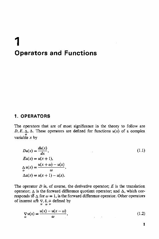
Operators and Functions
1. OPERATORS
The operators that are of most significance in the theory to follow are D, E , A, A. These operators are defined for functions u(x) of a complex variable x by
W
The operator D is, of course, the derivative operator; E is the translation operator; A is the forward difference quotient operator; and A, which cor- responds to” A for W = 1, is the forward difference operator. Other operators of interest a& V, 6, P defined by
W W W
v u ( x ) = u(x) - u(x - W )
9 W W

2 Chapter 1
u(x +&l) - u(x - $0)
u(x +h@) + u(x - $ W )
I W S u(x) =
El. u(x) =
W
W W
and known as the backward difference quotient, the central difference quo- tient, and the central mean, respectively. The corresponding operators for W = 1 are designated by V, S, p, respectively. These operators are capable of repeated application; thus
E2U(X) = E(Eu(x)) = Eu(x + 1) = u(x + 2),
A2u(x) = A(Au(x)) = U ( X + 2) - ~ U ( X + 1) + U ( X )
d2 dx2
D2 U ( X ) = D(Du(x)) = -u(x).
In general, one defines E' by E' u(x) = u(x + r )
for all complex r .
f l = l + w A
The following relation holds between the operators E and A : W
(1.5) W
thus, E' = (1 + W A)"", Ar= W"(P - l)'. (1 4
W W
In particular, from
U ( X + h) = (1 + W A ) h ' W ~ ( ~ ) (1.7)
and the binomial series, the following formal expansion (Newton's formula) is obtained:
W
U ( X + h) = 2 ( hy)o' A'u(x). W
j=o
This expansion plays the same role in the difference calculus as the Taylor series does in the differential and integral calculus. Clearly,
lim A u(x) = Du(x) (1 -9)
so that for W -+ 0, (1.8) goes over .to the Taylor expansion of u(x + h) about W+O W
A.
The differences of a function may be obtained from
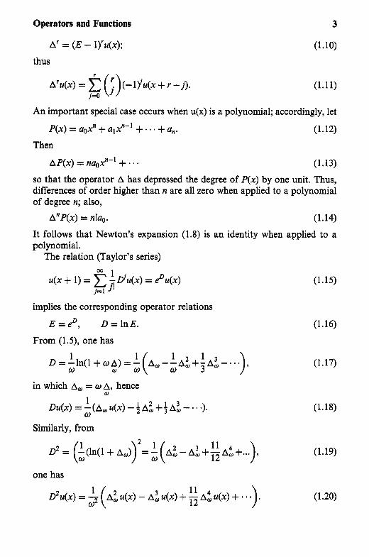
Operators and Functions 3
Ar = ( E - l ) r ~ ( ~ ) ; thus
A'u(x) = 2 (y)(-lyu(x + r - j ) , j=o J
(1.10)
(1.11)
An important special case occurs when u(x) is a polynomial; accordingly, let
P(X) = aox" + alY" + a . . + a,. (1.12)
Then
AP(x) = nuox"" + - (1.13)
so that the operator A has depressed the degree of P(x) by one unit. Thus, differences of order higher than n are all zero when applied to a polynomial of degree n; also,
AnP(x) = n ! ~ . (1.14)
It follows that Newton's expansion (1.8) is an identity when applied to a polynomial.
The relation (Taylor's series) m .
implies the corresponding operator relations
E = e', D = In E. From (1.5), one has
W
in which A, = o A , hence 1
W
Du(x) = 0 ( A , ~ ( x ) - f A i + 3 A i - * a).
Similarly, from
(1.15)
(1.16)
(1.17)
(1.18)
(1.19)
one has

4 Chapter 1
Formulae (1.18) and (1.20) are often useful for numerical differentiation. When applied to polynomials, they become identities.
2. FACTORIAL FUNCTION-STIRLING NUMBERS
Operations of the difference calculus are facilitated by use of the factorial function defined by
x(") = x(x - 1) ' ' (x - n + l), (1.21)
x@) = 1,
x(-d = 1 (x + 1) ' ' ' .(x + n)
for n 2 0 and integral. For general n, one defines x@) by [8]
(1.22)
in which r ( x ) is the Eulerian gamma function [8]. The salient feature of the function x@) is expressed in
Ax(") = nx("-') (1 -23)
whose proof is
The function x(") is related to the binomial by
(;) ==$
(1.24)
(1.25)
hence
(1.26)

Operators and Functions 5
Using the notation d o " for dx" at x = 0, Newton's formula provides the representation of x" in terms of factorials; thus
X" = CXO-A~O", n > 0. " 1 j ! j = 1
(1.27)
The name Stirling numbers of tlie second kind [g] is given to the coefficients in (1.27) and symbolized by Si; hence
(1.28) n
j = 1
Some special values are
s:=o, n > O ; S ; = I , n P O ; s',=o, j > n . (1.29)
x x o = xO'tl) + j x o (1 -30)
S:,, = S',-' +j . (1.31)
Expansion of X" and x " + * by means of (1.28) and use of
yield the relation
Using the initial conditions
s0=1, 0 $=o, j > O , (1.32)
the numbers S', may be obtained step by step. A short table of values is given in Table 1.
The inverse problem, that of expanding x@) in terms of d (1 5 j 5 n) for n > 0, is solved by use of Taylor's formula. Using the notation 0'0") for DX(") at x = 0, one has
(1.33)
The name Stirling numbers of the first kind is given to the coefficients in (1.33) and symbolized by $; hence
n
(1.34)

6 Chapter 1
Table 1: Stirling Numbers of Second Kind
n l j 1 2 3 4 5 6 7 8 9
1 3 1 7 6 1 15 25 10 1 31 90 65 15 1 63 301 350 140 21 1 127 966 1701 1050 266 28 1 255 3025 7770 6951 2646 462 36 1
Some special values are
g=o, n > 0 ; S;=I , n > O ; s ~ = o , j > n . (1.35)
(1 -36)
in (1.34) yields the relation
S',,, = &" -n SA, (1.37)
which, together with the initial conditions
S ~ = I , 0 $=o, j > O , (1.38)
permits step-by-step determination of $, . A short table of values is given in Table 2.
Table 2 Stirling Numbers of First Kind
1 2 3 4 5 6 7 8 n l j
1 -1 1 2 -3 1
-6 11 -6 1 24 -50 35 -10 1
-120 274 -225 85 -15 1 720 -1764 1624 -735 175 -21 1
-5040 13068 -13132 6769 -1960 322 -28 1

Operators and Functions 7
3. BETA FUNCTION-FACTORIAL SERIES
The Eulerian beta function [8], B(x, y ) is defined by 1
B(x, y ) = 1 f"(l - t)Y"dt, x > 0, y > 0
and can be expressed in terms of the gamma function by
in particular, AB(x, v) = -&, y + 1)
in which A operates with respect to x , and
in which j > 0 is integral. Expansions of the form
(1.39)
(1 -40)
(1.41)
(1.42)
(1.43)
are very useful in the solution of difference equations. They are called factorial series of the first kind. A Newton series of the form
(1.44)
is called a factorial series of the second kind. Both series are said to be associated.
The following theorems of Landau and Norlund whose proofs may be found in Ref. 8 provide some background on the nature of associated series. It is assumed that x is nonintegral. The symbol R(x) designates the real part of x .
Theorem (Landau): Associated series converge and diverge together.
Theorem (Landau): If a factorial series converges for x = xo, then it con- verges in the half-plane R(x) > R(xo), and converges absolutely in the half- plane R(x) > R(x0 + 1). If the series converges absolutely for x = xo, then it converges absolutely for R(x) > R(xo)
The preceeding theorems allow the introduction of the abscissa of con- vergence A and the abscissa of absolute convergence p. The following theo-

8 Chapter 1
rem of Landau provides the determination of h. To obtain p, the coefficients a, are replaced by la, 1 . Define a, B by
Then one has
Theorem (Landau): If h I: 0, then h = a; otherwise h = B.
rems. For the condition of uniform convergence, one has the following theo-
Theorem (Norlund): If the factorial series converges at x0 then it converges uniformly for
-+n+q<arg (x -xo)<h lc -q
in which q > 0 and arbitrarily small.
Theorem (Norlund): If the factorial series converges at xo, then it converges uniformly for
R(x) = R(x0) + E
in which E > 0 and arbitrarily small.
for assume Expansion of a function into a factorial series of the first kind is unique,
(1.46)
in which each series is assumed to converge in some right half-plane. Multiplying both sides by x and letting x + 00 yields a. = bo. Removing the terms corresponding to j = 0 and multiplying by x(x + 1) yields aj .= bj for all j > 0. Thus, an inverse factorial series can vanish identically only If all coefficients vanish. The uniqueness theory for Newton series is not as straightforward. Consider
n + 00, J=O
(1.47)
in which use is made of the asymptotic relation

Operators and .Functions
then
gW( x; l ) = 0, R(x) > 1, j = O
9
(1 -48)
(1.49)
= 1, x = 1, = 0 0 , R(x) < 1.
Thus, for R(x) =- 1, the series provides an example of a null series, Expansion, therefore, of a functionf(x) into a Newton series may not be unique. Nonetheless, the following holds true.
Theorem: Let f(x) be expansible into a Newton series with convergence abscissa h, and let it be analytic in the half-plane R(x) > I, then the expan- sion is unique if l p A c 1.
This may be proved by setting
F(x) = c A'F(1) j = O
W
(1 S O )
which is the assumed expansion forf(x). Because the expansion is valid for R(x) > h (h c l), one has F(j ) = f ( j ) (j 2 1) and hence
F(x) = 2 Ajf(l)( x 7 l ) j = O
(1.51)
so the expansion is unique. Thus, the convergence abscissa of null series must be greater than one.
Differences of n(x) (1.43) are readily calculated; thus
which follows from (1.41). In particular,
A'n(1) = (-1)' c ai W
j = l j + r + 1 '
from which the Newton expansion of n(x) is immediate.
(1.52)
(1.53)

10 Chapter 1
4. @-FUNCTION AND PRIMITIVES
For givenf(x), a function F(x) satisfying
= f ( 4 (1.54) will be called a primitive or a sum off@). In order to obtain a s u m of S2(x), it is necessary to introduce another important function of the difference calculus, the psi function. From the equation
r(x + 1) = xr(x) (1.55)
r’(x + 1) = xr(x) + r($. (1.56) satisfied by the gamma function, one obtains by differentiation
.Setting
(1.57)
one has, from (1.56) on division by r(x + l), 1
A+(x) = -. (1.58) X
Thus, this identifies +(x) as playing the same role in the difference calculus as ln(x) does in the infinitesimal calculus. Thus a primitive for Q(x) may be written
Let f ( x ) be expansible in a Newton series
f ( x ) = 2 A j f ( l ) ( x 7 l ) ; j=o
then a primitive is given by
(1.59)
(1.60)
(1.61)
Since r’(1) = - y ( y is Euler’s constant, y = 0.57721566), one has @(l) = -y; also, from (1.58),
(-1)i-l Aj+( 1) = - j
, j z 1 . (1.62)
Hence one has the following elegant Newton expansion:

Operators and Functions 11
(1 -63)
whose abscissa of convergence is h = 1. This series provides a practical means of computing $(x) to moderate accuracy for 1 5 x 5 2, from which, by use of (1.58), $(x) may be computed for other values of the argument.
An immediate application of the sum of a function is to the summation of series.
Let
A W ) = f ( 4 , (1.64)
(1.65)
Then, because AS, =f(n + l), (1.66)
one has
S, = F(x)l;+' = F(n + 1) - F(0). (1.67)
For example, let f ( x ) = x2; then, from the Newton expansion
x2 = ( 7 ) + 2 ( 3
one has
Thus
s n = k j 2 = ( j = 1 n + l ) + 2 ( n + l ),
(1.68)
(1.69)
(1.70)
S, = in(n + 1)(2n + 1). (1.71)
As another example, consider 1
f ( x ) =
and w 1
= 5io.m.
(1.72)
(1.73)
....................... . . . . . . . . . . . . , _ . . . . . . . . . . . . . . . . . . . . . . . . . . . . . . . . . . . . . . . . . . . . . . . . . . . . . . . . . . . . . . . . . . . .

12 Chapter 1
Since
one has
and S = F(oo) - F(1) = $ I
(1.74)
(1.75)
(1 -76).
5. LAPLACE AND MELLIN TRANSFORMATIONS
The Laplace and Mellin transformations are of particular importance in applied work. As many sources of information are available [10,1 l], only certain properties of the trapformations and transforms will be cited.
The Laplace transform, f ( s ) , of a function f ( t ) is defined by
(1.77)
for various classes of functions. The correspondence betweenf(t) andf(s) will be indicated by
f (0 "f f C 9 7 (1.78) where it is always assumed that f ( t ) vanishes for negative arguments. A useful class of functions is the class L defined by
1. f ( t ) is Riemann inte rable over ( E , T ) for arbitrary E 0 and T > E .
2. lim S,' ~f(t)ldt = io ~f(t)l dt exists. P 3. There exists so, real or complex, such that lim 1; e-""'ft) dt exists. 4. f ( t ) has only jump discontinuities in ( E , T).*-)OO
e+O+
A convergence theorem is the following:
Theorem: f ( t ) E L + (1.77) converges foz R($) > R(so) and defines a func- tion f ( s ) analytic in that half-plane withf(oo) = 0.
Define 4(t) by F t
(1.79)
Operators and Functions 13
Then integration by parts establishes
Theorem: f ( t ) E L =+ (1.80) converges absolutely for R(s) > R(s0).
Forf(t), g(t) E L, define h(t) by
(1.80)
(1.81)
Then h(t) E L and is called the convolution product off(t) and g(t). It is often symbolized by
h(t) =f@> * (1.82) An important property of the convolution product is expressed in
Theorem: Let the transformsf(s), &S) be convergent for the same so; then the transform, l&), of h(t) = f ( t ) * g(t) is convergent at so and
i(s) =?(is) * ,g($).
Concerning the convergence abscissa itself, one has the following results.
Theorem: If the convergence abscissa, h, satisfies h L 0 then
Theorem: Iff(t) 2 0, then the convergence abscissa, h, is a real singular point
A function, N(t ) , for which
l N ( 3 d u = 0, t L: 0
is called a null function. One has
Theorem: !(S) determinesf(t) to within a null function.
Table 3 gives a short list of operational properties (a > 0, f ( t ) = df(t)/dt). The bilateral Laplace transform
14 Chapter 1
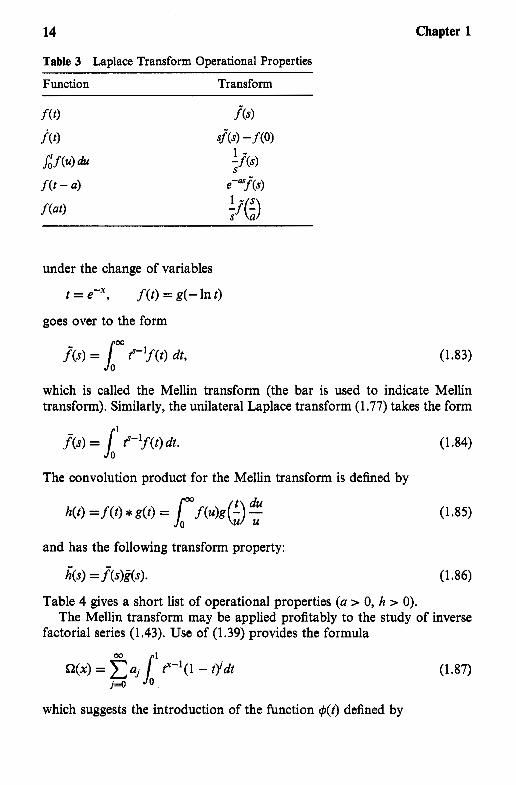
Table 3 Laplace Transform Operational Properties Function Transform
under the change of variables
t = e-', f ( t ) = g(- In t )
goes over to the form
f ( s ) = t""f(t) dt, 0
(1.83)
which is called the Mellin transform (the bar is used to indicate Mellin transform). Similarly, the unilateral Laplace transform (1 -77) takes the form
f ( s ) = 1 t""f(t)dt. (1.84) 1
0
The convolution product for the Mellin transform is defined by
(1.85)
and has the following transform property:
i ( 8 ) =f(s)&). (1.86)
Table 4 gives a short list of operational properties (a > 0, h > 0).
factorial series (1.43). Use of (1.39) provides the formula The Mellin transform may be applied profitably to the study of inverse
(1.87)
which suggests the introduction of the function #(t) defined by
Operators and Functions 15
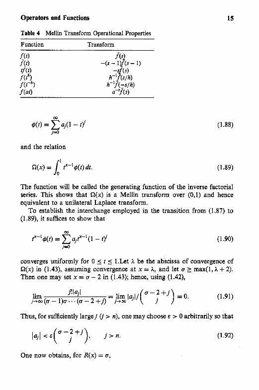
Table 4 Mellin Transform Operational Properties
Function Transform
(1 3 8 ) j=O
and the relation
(1 -89)
The function will be called the generating function of the inverse factorial series. This shows that a(x) is a Mellin transform over (0,l) and hence equivalent to a unilateral Laplace transform.
To establish the interchange employed in the transition from (1.87) to (1.89), it suffices to show that
W
t"#(t) = cujr"-'(l - tr' j=o
(1.90)
converges uniformly for 0 I t I 1.Let h be the abscissa of convergence of Q(x) in (1.43), assuming convergence at x = h, and let a L max(1, h + 2). Then one may set x = a - 2 in (1.43); hence, using (1.42),
(1.91)
Thus, for sufficiently largej (j > n), one may choose E > 0 arbitrarily so that
One now obtains, for R(x) = a,
(1 -92)

16
< &tu-l( l - (1 - t))-+l < E .
As an example of the use of (1.89), consider W
n(x) = c dx(-J), j= 1
One has W
n(x) = a C dX(7j - l ) ; j=O
define
Then comparison with (1.42) provides
For another example, consider the expansion of l/x2. Because
1 X2
1 - = -l t x - l l n t dt
one has
and thus
Chapter 1
(1.93)
(1.94)
(1.95)
(1.96)
(1 -97)
(1.98)
(1.99)
(1.100)
The generating function $(t) of the product of two series nl(x), n2(x) whose generating functions are respectively &(t), ~ $ ~ ( t ) is, by (1.85),
= 41 ( 0 * 4 2 ( 0 (1.101) in which one must observe that r#q(t), q52(~), 4(c) = 0 for t 0, t > 1.

Operators and Functions 17
6. SOME OPERATIONAL FORMULAE
To conclude this brief summary of operators and functions useful in differ- ence equation theory, certain operational results concerning the operators E and D will be presented. It is useful to think of f ( x ) in terms of a power series expansion in powers of x , then, since
El = 1, (1.102)
(1.103)
(1.104)
(1.105)
Because, more generally,
E[a"u(~) ] = O ~ + ' U ( X + 1) = aX(aE)u(x), (1.106) the shift formula follows, namely
f(E)[a"u(x)l = a'lf(aE)u(x>. (1.107)
The corresponding results for the operator D may be derived indepen- dently or from the preceeding results for E by using the relation (1.16). They are
f ( D > 1 = f ( O ) , (1.108)
f(D)[e""u(x)] = e"f(D + a)u(x). (1,109)
Examples of these operational formulae will arise in the exercises and in later applications.
PROBLEMS
1. Solve d ( x ) + 3u1(x) + 2u(x) = xe+, D.
2. Solve
u(x + 2) - 3u(x + 1) + 2u(x) = x23x.
3 . Show

18 Chapter 1
4. Show (Euler's transformation) 1 1 a o - a l + a z - . ' . = 5 a o - F A a o + ? A 1 ' 2 ao - " . .
2 5 . Show
A" sin(ax + b) = (2 sin
A" cos(ax + b) = (2 sin -)" a cos [ ax + b + n "$7. a + 2
6 . Show
n! W
,x+ l)...(x+n)=~n:;'~l(xI'>.
7. Show (Vandermonde)
(x + h)'"' = 2 (;)x("-Jw. j = O
then show
j = O j + l
10. Show
and, hence,
Operators and Functions 19
11.
12.
13.
14.
W
D'f(0) = c S; W"" A f ( 0 ) . n=r n! W
Hint: Consider the derivatives of (1 + t)" with respect to x. Show (Stirling)
Show
and, hence,
Hint: Consider the differences of exf with respect to x . Show (the transformation x -+ x + m)
Hint: Replace the generating function +(t) by t-"+(t) Let.
then show m
G?'@) = - C bjB(x,j + 1) j = 1
in which j - 1
b j = C - . a, v=o j - v

20 Chapter 1
15. Show 1 1 1 x x + l x + 2
m ”- +“.I I = c 2-j”B(x,j + l).
j = O
16. Show (Waring’s formula) 1 1 a ”- +- + a(a+l) +..., x - a - x x(x + 1) x(x + l)(x + 2)
17. Show 1 1 1 1 1 x 2x(x+ 1) 6x(x+ l)(x+2)
Alnx=”---”--- - . . . Hint: A lnx is the Laplace transform of (1 - e-’)/Y.

2 Generalities on Difference Equations
1. GENESIS OF DIFFERENCE EQUATIONS
By the genesis of a difference equation is meant the derivation of a differ- ence equation valid for a given family of primitives. Consider the equation
F(x, u(x>,p(xN = 0, (2.1) in which p ( x ) is an arbitrary periodic function of period one, and the equa- tion
F(x+l ,u(x+l ) ,p(x) )=O. (2.2) Elimination of p(x) from (2.1) and (2.2) yields a relation of the form
G(x, u(x), u(x + 1)) = 0. (2.3)
Equation (2.3) is a difference equation satisfied by every member, u(x), of the family defined in (2-1). Because only the arguments x, x + 1 occur in (2.3), the equation is said to be of first order.
The following are examples of this procedure. Consider the family
u(x> = p(x)g(x). (2.4) Then, from
21
22 Chapter 2
one has
g(x)u(x + 1) - g(x + l)u(x) = 0. Important special cases are the choices g(x) = d" and g(x) = a"T(x + l), for which one obtains
u(x + 1) - au(x) = 0, (2.7)
#(X + 1) - -u(x) = 0, x+l a
respectively. These correspond to the geometric distribution (1 - a)& ( x = 0, 1,2, m ) and the Poisson distribution, +(x, a) , defined by
The function @(x, a)-' satisfies (2.8) with initial value u(0) = ea. Similarly, setting g(x) = d"/r(x + l), one has
(2.10)
satisfied by @(x, a) itself with initial value u(0) = e-". The difference equations may be used as recursions for the successive
Computation of u(x) at integral points. These values, in turn, may be used to form the differences at, say, x = 0, from which a Newton expansion (1.8), with W = 1, may be constructed: thus, values of u(x) may often be readily obtained at non-integral points. Systematic exploitation of this idea occurs in Chapter 5;
Another example is provided by 1 u(x) = -
P ( X > - x from which follows
A X-- [ u;x,l = O
(2.1 1)
(2.12)
and, hence, u(x)u(x + 1) + u(x + 1) - #(X) = 0. (2.13)
This is a special case of the general Riccati equation
u(x)u(x + 1) + a(x)u(x + 1) + b(x)u(x) + c(x) = 0. (2.14)
The Clairault difference equation is obtained on considering

Generalities on Difference Equations 23
= XP(4 + f @ ( X N (2.15)
in whichf(x) is prescribed. One has
= P(X> (2.16) and, hence,
U ( X ) = XAU(X) +f (Au(x) ) . (2.17)
A two-parameter family, that is, a family in which two arbitrary periodics pl(x),p2(x) occur, has the form
F(x, u w , Pl(49 P2(X)) = 0. (2.18) Use of
(2.19)
together with (2.18) provides the relation
G(u(x), u(x + 11, u(x + 2)) = 0 (2.20)
which, because of the arguments x , x + 1, x + 2 is called a difference equa- tion of second order. In general, when F = 0 contains n arbitrary periodics, p l ( x ) , . . .p&), a difference equation of nth order is obtained.
Consider the equation
44 = P1 ( 4 a " + P2(X)bX (2.21)
and the additional equations
(2.22)
Then elimination of pl(x)a",p2(x)bX considered as unknowns provides the determinant
(2.23)
and, hence, the second-order difference equation
u(x + 2) - (a + b)u(x + 1) + abu(x) = 0. (2.24)
Illustrations of difference equations arising from model formulations are plentiful. The following are some examples.

24 Chapter 2
2. THE M / M / C BLOCKING MODEL
A Poisson arrival stream of a Erlangs is offered to a fully available trunk group consisting of n independent exponential servers. Let u(n, j ) designate the probability that, at an arbitrary instant of time with the system in equilibrium, j trunks are busy. Then the balance equation for flow into state j is
(j + l)u(n,j + 1) - (j + a)u(n, j ) + au(n, j - 1) = 0, 1 s j n - 1,
u(n, 1) = au(n, 01, 2 u(n,j) = 1. j=O
(2.25)
The quantity B(n, a) = u(n, n), which is the probability that all trunks are busy, is called the Erlang loss function; it satisfies the following difference equation:
B(n + 1, a)" = -B(n, a)" + 1, B(0, a) = 1. n + l a
(2.26)
3. THE M/M/I DELAY MODEL
A Poisson arrival stream of a Erlangs is offered to an exponential server with unit mean service rate. Let u(x, t ) designate the probability that there are x units in the system at time t if the system was empty at t = 0. One has
w x , t ) at " - u(x + 1, t ) - (1 +a)u(x, t ) + au(x - 1, t),
" t, - au(0, t ) + u(1, t), u(0,O) = 1, at (2.27)
x=o
Equation (2.27) provides an example of a differential-difference equation. In many forms of stochastic modeling, the generic form of equation expressing time dependence is
" au(x7 t, - Lu(x, t ) at
(2.28)
in which L is an operator with respect to x. Such equations are often said, to be of Fokker-Planck or semigroup type [12].
Generalities on Difference Equations 25
4. THE TIME HOMOGENEOUS FIRST-ORDER MODEL
A function Z(t; z ) with Z(0; z ) = z is required that satisfies A z(t; Z) = q q t ; z)) (2.29) 0
in which the function O(z) is specified. This includes the usual one-dimen- sional theory of branching processes [12,13]. In this role Z(t; z ) considered as a function of z corresponds to the probability generating function of the population distribution at the tth generation when t is an integer; otherwise it corresponds to continuous time branching processes. This equation is studied in Chapter 5 .
For further discussion of stochastic modeling, one may refer to Refs. [l2 to 141.
5. THE EULER EQUATION
As an illustration outside the field of stochastic modeling, one may consider the problem of the extremization of the functional [15,16]
n
S = c F(j, uU), VU)), v(j) = Au(j). (2.30)
The function F(x , U, v) is prescribed and it is supposed that suitable bound- ary conditions have been specified. It is required to determine ~ ( t ) (0 5 t 5 n). Differentiation of S with respect to ~ ( t ) yields the following Euler equation:
j=O
(2.31)
in which A operates with respect to t.
many examples of difference equations. In addition, the various dynamic programming formulations [l61 provide
A homogeneous linear difference equation of order n has the form an(x)u(x + n) + a,-l(x)U(x + n - 1) + * ’ + ao(x)u(x) = 0. (2.32)
The solution U(X) = 0 will be excluded from consideration in what follows. It will be assumed that the coefficient functions aj(x> (0 5 j 5 n) have only essential singularities because, otherwise, multiplication of the equation by a suitable entire function will remove all poles.
The following are called the singular points of the difference equation: the zeros of ao(x) and an(x - n) and the singularities of aj(x) (0 fj f n).
. . . . . . , . , . . , . , . . . _ , , ” .,.,.,.,,,,,..,,.......~.. ~ . . I . . . . . . . ..
26 Chapter 2
Given any point a, x is said to be congruent to a if x - a is an integer, otherwise incongruent.
The principal interest concerning (2.32) lies in finding analytic solutions. If x is restricted to be integral, then the conditions of a solution satisfying, say, prescribed initial conditions may be relaxed. In this case, the equation may be considered to provide a solution through sequential computation and may more properly be considered a recursion.
Considering the second-order equation az(x)u(x + 2) + a1(x)u(x + 1) + ao(x)u(x) = 0 (2.33)
to be typical, and solving for u(x), one has
If u(x) is prescribed for 0 5 R(x) 2, then, for values of x incongruent to the zeros of ao(x) and the singularities of the coefficients, u(x) may be continued to the left. Similarly, by considering
(2.35)
if x is incongruent to the zeros of az(x - 2) and the singularities of the coefficients, then u(x) may be continued to the right. Thus u(x) may be continued throughout the plane except at points congruent to the singular points of the equation.
A set of functions ul(x), , U&) satisfying (2.32) is said to form a fundamental system of solutions if there is no relation of the form
Pl(X)Ul(X) + ' ' ' +P"(X)U,(X) = 0 (2.36) such that for at least one x incongruent to the singular points of (2.32), the p j (x ) are not all simultaneously zero. The pj(x) are, as introduced earlier, periodics of period one. One then has that all solutions of (2.32) are spanned by u1(x), - , U&). The following theorem of Casorati enables one to deter- mine whether a given set of solutions constitutes a fundamental system.
Theorem (Casorati): The necessary and sufficient condition that the set ul(x), . - . ,u , (x) should be a fundamental system of (2.32) is that the Casorati determinant
u1(x) * * "U,(X)
U l ( X + l)*.*u,(x+ 1)
u1(x+n- l ) * * * u , ( x + n - 1)

Generalities on Difference Equations 27
should not vanish for any value of x incongruent to the singular points of (2.32).
ProoJ The condition is necessary, for let U,(x) (1 I j I n) be the cofactors of the last row, then
c U j ( X ) U@) = 0, i= 1
n
(2.37)
c .j(X + n - l)Uf(X) = D(x) = 0, i=l
in which the last equation follows by assumption. Now Ui(x + 1) are the cofactors of the first row, hence
n
i= 1 c U i ( X ) U i ( X + 1) = D(x) = 0,
(2.38) n
i= 1 c Ui(X + n - l)Ui(X + 1) = 0.
Equation (2.37) determines Ui(x ) /Ul (x ) (2 5 i 5 n) and (2.38) determines Ui(x + l)/Ul(x + l), hence
Thus one may set
"- UdX) PdX) U1 ( x ) - P1 ( x )
and consequently, from (2.37),
(2.39)
(2.40)
PI (~1.1 ( X ) + * + Pn(x)un(X) = 0 (2.41)
showing that u1(x), . , un(x) does not form a fundamental system. To establish the sufficiency of the condition, assume u1 ( x ) , m e . , un(x) does
not form a fundamental system, so that a point Q incongruent to the singular points of (2.32) and a set of periodics pl(x), - ,p&), not all zero at a, can be found for which
then one also has
(2.42)

28
Thus
D(a) = 0
and the theorem is proved.
Chapter 2
(2.43)
(2.44)
Application of Casorati's theorem to (2.24) for which a", b" are known solutions yields
D(x) = axbx(b - a), (2.45)
which, for a # b, never vanishes; hence a", b" constitute a fundamental system. However, in contrast, for the system ax sin 2nx, b", one has
D(x) = d"bX(b - a) sin 2nx (2.46)
which vanishes for all integral values of x. Thus this does not form a funda- mental system.
As another example, consider the equation
u(x + 2) - xu(x) = 0
for which a solution set is
For the Casorati determinant, one has
(2.47)
(2.48)
(2.49) = ( - -1)~+~4&r(~) .
Because D(x) does not vanish at points incongruent to the singular point x = 0, the set (2.48) constitutes a fundamental system.
Casorati's theorem enables the general form of the solution of (2.32) to be obtained. Thus, let ul(x), . , un(x) be a fundamental system; then, from
i=O
2 ai(x)uj(x + i) = 0, 1 r j 5 n, i=O
on eliminating the coefficient functions, aj(x) (0 5 i 5 n), one has
(2.50)

Generalities on Difference Equations 29
I = o . (2.51)
The minors of the elements of the first column are not zero because ul(x), , un(x) form a fundamental system, hence periodics p(x),pl(x), , pn(x) exist for which
p(x)u(x) +P1 (4u1 (x) + ' ' * + Pn(x>ufl(X> = 0 (2.52) with p(x) # 0; hence one may also write
4x1 = P I ( X ) U ~ ( X ) + * m * +pn(x>un(x>- (2.53) Thus (2.53) provides the general form of solutions of the nth order, homo- geneous, linear difference equation (2.32). The importance of a fundamental system is now evident.
The determinant of (2.51) may be used to construct a difference equation admitting a given fundamental set of solutions. For example, given ul(x) = x, u2(x) = 2' one has
I u(x + 2) x + x 2 2x+2 2 x l u(x+ 1 ) x + 1 2x+1 = o , (2.54)
and hence the equation is
( x - l)u(x + 2) - (3x - 2)u(x + 1 ) + 2xu(x) = 0. (2.55)
The corresponding Casorati determinant is
D(x) = 2'(x - 1 ) . (2.56)
Because the singular points are 0, 1 and D(x) does not vanish at points incongruent to 0, 1, the system x, 2' is verified to be a fundamental system. One also has, from (2.53), that all solutions of (2.55) have the form
u(x> = P l ( X ) X +P2(x)2x. (2.57) A remarkable result exists for Casorati's determinant for a given differ-
ence equation, namely that it satisfies a first-order equation. That is the assertion of Heymann's theorem.
Theorem (Heymann): Casorati's determinant, D(x), satisfies

30 Chapter 2
(2.58)
Multiply the first row by al(x)/an(x), and the second row by a2(x)/an(x) up to the (n - 1)st row by an-l(x)/an(x); add the resulting rows to the last row. From (2.32), one has
hence the last row of D(x + 1) becomes
(2.60)
Transferring this to the first row of the determinant establishes the theorem.
It immediately follows from Heymann’s theorem that if D(x) vanishes at a point a then it vanishes at all points congruent to a.
A criterion in terms of asymptotic behavior (x + 00) for ascertaining that a given system of functions constitutes a fundamental system is con- tained in the following theorem.
Theorem (Milne-Thomson): If
in which r goes through the positive integers, then the system ul(x), . - e , U&) is fundamental.
Proof. It is supposed all the functions uj(x) exist in some half-plane. Suppose they are not fundamental; then one may write
~l(x)ul(x)+’..+~n(x)un(x)=O (2.61) in which not all pj(x) (1 5 j 5 n) are zero. Let p,($ be the last nonzero periodic; then
Pl(X)Ul(X) + * . * +P,(X)U,(X) = 0. (2.62) Thus, on dividing by u,(x + r ) ,
(2.63)
Generalities on Difference Equations 31
Letting r -F bo in (2.63) and using the stated value of the limits, one obtains p,(x) = 0, which is a contradiction.
When the asymptotic behavior of solutions of difference equations is known, this result can be usefully applied.
PROBLEMS
1 .
2.
3.
4.
Form the difference equations satisfied by the following families:
u(x) = p(x)2x, u(x) = XP(X> + 1 &(x) + 1
Form the Euler equation for the minimization of n
S = c (u(j)2 + w ( j y > , 2 u(0) = z. j=o
Show that the second-order difference equation whose solutions are
is
( x - a)(x - a + l)u(x + 2) - (2x + l ) (x - a)u(x + 1 ) + x%(x) = 0;
also show
Using the asymptotic criterion of Milne-Thompson,. show that the func- tions uI(x) , u2(x) of Prob. 3 form a fundamental system.

Norlund Sum: Part One
1. INTRODUCTION
The basic problem to which we now turn our attention is the solution of the equation
for primitives F(xlw) given +(x), This constitutes a generalization of the corresponding problem of the integral calculus, namely the discovery of primitives F(x) satisfying
DF(x) = +(x). (3.2)
Progress in the integral calculus was impeded until a constructive defini- tion was framed providing one of the primitives of (3.2). This definition- the Riemann integral-formed the foundation for the theory of integration. Its properties allowed a fruitful theory to be developed. Similarly, one would like a constructive definition of a particular primitive of (3.1) that would possess rich analytic properties permitting a useful theory to be developed. It should provide simple representations of important functions and have means of ready asymptotic computation and approximation. For example, certainly F(xlw) corresponding to +(x) being a polynomial should also be a polynomial; such a primitive exists, as can be seen from the Newton expan- sion (1.8). The unique determination of F(xlw) should rest on its value at a
32

Norlund Sum: Part One 33
single point rather than a specification throughout an interval, and one would also like lim F(xlo) to reduce to a solution of (3.2) because lim Af(x) = Df(x) whenever Df(x) exists. w-*o W
which will now be studied.
W+O
All these properties are provided by the formulation of Norlund [17],
2. PRINCIPAL SOLUTION
The definition of the principal solution of Norlund will be given in two stages. In order to motivate the definition, (3.1) is rewritten in the form
using (1.6). Thus W
F(xlw) = -- #(x) 1 -E* = -[l + E" + E2W + - - +]@#(X), (3.4)
Formally, (3.4) is a solution of (3.1), although, without restricting +(x), the series need not converge. It was found by Norlund, however, that the desired properties were not given by (3.4) without the addition of a suitable constant. The constant chosen is
in which a is arbitrary. A firm motivation for this choice will emerge when the definition is completed in the second stage. Accordingly, one has the following definition.
Definition (Norlund Principal Solution): Let both the integral and sum con- verge. Then the principal solution of
A F(xlo) = #(x) W
or sum of #(x) is
The notation introduced by Norlund for the principal solution is
34 Chapter 3
X
F ( x J o ) = S #(z) A z W
and the operation is referred to as “summing @(z) from a to x.” The nota- tion F(x) is used when W = l. The quantity W is called the “span” of the sum and, unless otherwise stated, is assumed to be positive. I
Examples of evaluations directly from the definition are
in which
is the generalized zeta function [18].
3. SOME PROPERTIES OF THE SUM
A number of properties of the sum flow directly from the definition, that is, from
(3.10)
One has, of course, X
A S #(z) A z = #(X) . (3.1 1) w a W
Quite simply, one obtains from (3.10) the following relations:
X
S #(z + b) A z = S #(z) A z; x+b
W a+b W
also, for W 0, one may write X X l W
(3.12)
(3.13)
(3.14)

Norlund Sum: Part One 35
in which, as is usual, Ay refers to a unit increment. Let m be a positive integer; then substitution of x + vw/m (0 5 U 5 m -
1) in succession for x in (3.10) and addition of the resulting equations yield m- 1 c F(x +:la) = mF(--). W V=O
(3.15)
This is called the multiplication theorem of the principal solution. The origin of the name will become evident when application is made to special func- tions such as the Bernoulli polynomials and the gamma function.
Let E > 0 be arbitrarily chosen; then, for the next result, the assumption will be made that +(x) = O ( X - ’ - ~ ) for x + 00. Let n be a positive integer and let A = no; then
m n
W c +(x + j W ) = W c +(x +]W) + W +(x + j W ) j=O j=o jzn
n (3.16) = W c +(x +jo) + O(W c ( x +jw)-””.
Use of an integral comparison gives
j=o j=O
uniformly for x 2 0. Thus, for fixed A,
and, hence, letting A -+ 00,
(3.17)
(3.18)
(3.19)
From (3.10), one now has
Of course this is what was desired because it provides a solution of (3.2). Also, clearly,
lim - c F ( x + 2 I w ) = --l F(tlo) dt. 1 m-l 1 x+o
m+m m u=o m X (3.21)
36 Chapter 3
The integral in (3.21) is called the span integral. Dividing (3.15) by m, letting m + 00, and using (3.20) and (3.21), one obtains the following theorem under the condition $(x) = O(x-"'):
F(tlw) dt = $(t) dt. 0
(3.22)
The results of (3.20) and (3.22) already provide justification for the inclusion of the integral in (3.10).
In (3.22) let x = a; then
6'" F(tlw) dt = 0. (3.23)
An immediate application of (3.23) is the following: Let G(xlw) be a primi- tive of (3.1); then the principal solution is of the form
F(xlw) = G ( x ~ w ) + C (3.24)
for some constant c. Substitution into (3.23) determines c and yields the formula
1 M+O
(3.25) F(xlw) = G(xlw) I f ,
in which the convenient notation of a vertical bar is used to represent the computation. Thus, one may construct the principal solution given any primitive. This is analogous to the evaluation of lox #(t) dt from a solution of DF(x) = $(x).
An example is given by the equation
A G(xlw) = xe-", S > 0. (3.26) 0
Using (1.6), this may be written
and hence one has
G ( x ~ w ) = - EO - 1 W xe-ax
(3.27)
(3.28)
(3.29)
by the shift formula of (1.107). Using (lS), one now has
Norlund Sum: Part One
1 G(xlw) = I - e-am(1+ w a)' x.
W
Expansion of (3.30) into positive powers of A yields W
37
(3.30)
(3.31)
Finally, using (3.25), one obtains
It may be observed that (3.32) could also be obtained from (3.7) by differ- entiation with respect to S.
4. SUMMATION OF SERIES
The summation of series is accomplished by the following identity, easily derived from (3.10):
An example is provided by (3.8), from which one has
x+no X n-l S Z - ~ A Z - S Z - ~ A Z =
1 a w a w C ( x + j W ) v * j=O
and hence
in particular, for x = 1, W = 1,
j=1 J
in which ((U) = ((U, 1) is the ordinary Riemann zeta function.
(3.33)
(3.34)
(3.35)
(3.36)

38 Chapter 3
5. SUMMATION BY PARTS
A[u(x)w(X)] = U(X) A W ( X ) + V ( X + W ) A # ( X ) (3.37) W W 0
one obtains
Now, applying (3.25) to A[u(z)v(z)] W yields the result +W
6 A[u(z)v(z)] = u(x)v(x) - u(t)w(t) dt = u(z)w(z) l:, (3.39) a w
which, incidentally, on comparison with (3.1 1) shows that the OperatorSA, S do not commute. Finally, using (3.39) in (3.38) and rearranging the tefms, one obtains the formula for summation by parts.
It may be observed that the limit of (3.40) for W ”+ O+ becomes the usual formula for integration by parts in the infinitesimal calculus. A simple example is given by
x 1
S zqz + 1) A z ,
Here, one may set
1 1 u(x) = - w(x) = - - *
X ’ X ’
hence, on applying (3.40),
Combining the two sums gives
(3.41)
(3.42)
(3.43)
(3.44)

NZirlund Sum: Part One 39
6. DIFFERENTIATION
The formula for differentiation of the sum follows readily from (3.10); however, to justify the operations, the assumption is now made that 4'(x) = O(x-'-') for some E > 0. One obtains
(3.45)
For example, consider
One has F'(x) = 1 - SF(x)
and hence 1
~ ( x ) = + ce-". The constant, c, is now determined by use of (3.23); thus
1 e-SX F(x) = - - - 8 l-e-' '
(3.47)
(3.48)
(3.49)
This result may be compared with (3.7).
7. EXTENSION OF DEFINITION OF SUM
In order to extend the range of application of the definition of the principal solution of (3.1), a summability approach will be taken. The summability factor e-Ax will be used-this is Abel summability. Accordingly, one has the second stage of the definition.
Definition (summability form): For A. 0,one defines X
s 4 ( z ) A z = W A+O+
lim 5 a
A z W
whenever the indicated limit exists. It is ossible in the general theory to use other summability factors such
as e-"but for the purposes of this treatment the preceeding definition suffices. A function $(x) for which the sum exists will be said to be summa- ble. Clearly, in this extended sense, (3.1 1) is still valid. In fact, all properties established for the sum to this point remain valid including the differentia-

40 Chapter 3
tion rule (3.45), which follows from the summability procedures applied to the derivative of e-"#(x).
As immediate examples of the definition, one may evaluate S + O+ in (3.7) and (3.32) to obtain, respectively,
(3.50)
Clearly, repeated application of summation by parts now shows that the sum of a polynomial is a polynomial. This fact will again be brought out in the study of Bernoulli polynomials, when an explicit solution will be given.
The asymptotic behavior of the sum in (3.10) for small h > 0 when applied to e-hx4(x) is closely imitated by the behavior of the corresponding integral term. Thus, even if the limits, h + 0+, do not exist individually, the limit of the difference of integral and sum can exist. This provides the basic motivation for the inclusion of the integral in the definition of principal solution.
8. REPEATED SUMMATION
The definition of the repeated principal sum is
Fn(xlw) = wn-l S x ( ( x - - ' ) q 5 ( ~ ) A Z . n - l 0
It will now be shown that
bn Fn(xIw) = #(X)*
One has
The identity (1.26)
(3.51)
(3.52)
(3.53)
(3.54)
used in the second term of (3 .53 ) yields

Norlund Sum: Part One 41
(3 .55)
(3 .56)
(3.57)
(3.58)
9. SUM OF LAPLACE TRANSFORMS
Quite often functions to be summed are, in fact, transforms, so it is of interest to obtain a representation for their sum. This representation will enable accurate numerical computation to be performed and will also permit the derivation of accurate bounds. Accordingly, let
f ( z ) = LW e-''f(t) dt (3.59)
which is assumed to converge absolutely for z 0, and let x 2 a 0, then one has the following.
Representation Theorem:

42 Chapter 3
Proof In order to establish the representation, the extended definition of the earlier section will be used. For the construction of the sum, consider first jaw e-Auf(u) du; one has
e-Auf(u) du = SW e-" du P e-"Y(t) dt a 0
(3.60)
is justified by the absolute convergence off(z) for z > 0. I M for some constant M uniformly for z 2 U , the series
j=O
is absolutely convergent; also, because
(3.61)
(3.62)
the series is absolutely and uniformly convergent for t 2 0. One now has
Setting
and hence X
Sf (z) A z = lim F(h + t ) f ( t ) dt. o h+O+ P 0
(3.63)
(3.64)
(3.65)
(3.66)
Norlund Sum: Part One 43
The function F(y) is continuous for all y E [0,00] with
F(0) = x - a - 4 W , F ( W ) = 0. (3.67)
Hence lim F(A + t ) f ( t ) = F(t)f(t) . 1+0+
(3.68)
Further, for A 2 0, t 2 0, one has IF(h + t)l 5 M uniformly in A, t; also, for h 2 0, t 2 E > 0, 0 < S a, one has lF(A + t)eg') 5 M uniformly in h, t; hence
( W + t)f(OI 5 Me-6f V(t)l (3.69)
uniformly for A 2 0, t 2 0. Because this is integrable on [0, m), one now has
A z = LW F(t)f(t) dt , (3.70) W
which is the stated representation.
The following are examples of the representation formula:
x lnz S - A z = - L 1 z o (';"- 1 we-x' - e-01 ) ( y + In t) dt
W -t
(3.71)
(3.72)
(3.73)
in which y is Euler's constant. The case v = 1 of (3.71) defines the general- ized $-function $(xlw), that is,
The case W = l is the ordinary $ - function,(l.57); thus,
X 1
1 Z t 1 - c t
+(xll)=$(x)=S-Az=Lw(T--- -I e-x' ) dt. (3.75)
The integral of (3.75) is called the Gauss representation. One may express $ ( X ~ W ) in terms of $(x) as follows. From (3.74), one has
(3.76)

44
obtained from the substitution z = ay. Also,
and hence
+(xlw) = In w + +(:)
I O . HOMOGENEOUS FORM AND BOUNDS
The identity (3.12), namely
X X
Chapter 3
(3.77)
(3.78)
(3.79)
indicates that one may profitably study the form
X
H(xlw) = S #(z) A Z. (3.80) X W
This form has a number of useful properties, among which is convenience of numerical evaluation, as will become apparent in this chapter. The differ- ence and derivative of H(xlw) have simple forms; thus,
=-SC#J(Z+W)AZ-"~C$(Z)AZ 1X 1 X
@ X W w x W
= S " 4 ( z + w ) - 4 ( z ) A z X w W
X
= S A +(z) A Z. x u W
To determine H'(xlw), one may differentiate
(3.81)
(3.82)
to obtain

Norlund Sum: Part One 45
CO
H’(x1w) = +(x) - w c q’(x + j w ) j=O
(3.83)
X
= S #’(z) A z. W
The generalization of (3.83) by use of summability is as follows:
~ ( x l w , A) = i e-Az4(z) A z; (3.84) W
hence, by (3.83),
Letting A + 0+, one again obtains X
H’(xlo) = S #J’(z) A Z. (3.86)
It is now seen that the opyators A and D commute with S .That could
X W
X
have been expected because S comm%es with translation, th; is,
x+a X
x f a W x S ~ ( z ) A z = S ~ ( Z + ~ ) A Z .
W (3.87)
Bemuse e-” is the eigenfunction for A andD, one expects this also to hold for S . Indeed, setting
W
X
1 1 Ab)=--- y 1 - e-7’
(3.88)
one has from (3.7),
i e+ A z = wA(wa)e-ax (3.89)
so that the corresponding eigenvalue is oh(&). The representation formula of the earlier section now takes the form
W
showing that Sf(z ) A z is itself a Laplace transform. x ,
X W
(3.90)
46 Chapter 3
To proceed further, it is important to determine properties of A@). A useful inequality for this purpose is Jensen's [ 191; that is, let f ( x ) be convex for x in an interval I and let p(x) I. 0 for x E I , then
Thus, from
follows
1 - e-y 2 ye-Y/*.
One has, from (3.88),
(3.91)
(3.92)
(3.93)
(3.94)
and hence, using (3.93),
1 1 A'@) 1. -?+F = 0. (3.95)
Because h(0) = -B, )\.(m) = - 1, the monotone decreasing character of Ab) establishes
(3.96)
Bounds for H(xlw) may now be obtained from the representation of (3.90). Let If(t)I 1. M , then, since
In? - +(X) = - / e-"wA(ot)dt 2 0, 00
W W 0
one has
(3.97)
(3.98)
and from

Norlund Sum: Part One
and
47
(3.99)
(3.100)
(3.101)
Equation (3.99) also implies the useful inequality 1
@(x) I lnx--, x > 0. 2x (3.102)
A further result is obtained from (3.100) on assumingf(t) p 0, thus, from (3.961,
x , ! f ( ~ ) A z 5 - 4 ~f (x ) . (3.103) a,
It is clear, from (3.59), thatf(t) L 0 impliesf@)(z) is of constant sign for
(- l)Y@)(z) p 0, r = 0,1 ,2 , . (3.104)
Such a function is called completely monotone. The Bernstein theorem [l l] implies that if f ( z ) is completely monotone for z > 0, then_ f ( t ) L 0; hence the condition for (3.103) may be restated in terms of f ( z ) , namely the requirement that f(z) be completely monotone.
It will now be shown that A Q ) is convex for y E [0, m). This will permit the construction of an accurate lower bound for H(x1w). Direct calculation shows that
z > 0 and alternates with respect to r, that is,
(3.105)
It is sufficient to show that A”Q) p 0 for y p 0. Setting 1 - e-y = a so that 0 5 a 1, one has
2 A’IQ) = (1 - .)(2 - 4 ,
[- ln(1 - - a3 ,
thus A”@) 2 0 is implied by
[- - 41 2 (1 - a)(2 - a) -
(3.106)
(3.107)
48 Chapter 3
The corresponding power series expansions are -ln(l -a> . [ a ] =Ea,"* j = O
m
Since
one has
with
thus,
Observing that 1 2 2
one may write a, in the form
2 j 1 k+l 1 2 j 1 k+l 1 a . - - " j + 3 2 j + l - k C-+""-c. I= 1 1 1 + 3 ~ = ~ k + 2 , = ~
(3.108)
(3.109)
(3.1 10)
(3.1 11)
(3.1 12)
(3.113)
(3.1 14)
One further modification of the form for aj is needed. It is observed that
generates the coefficients j
&+ 1 - k
(3.115)
(3.1 16)

Norlund Sum: Part One 49
and hence, from (3.11 l),
The final form for ai is now
(3.1 17)
(3.118)
Since the double sum of (3.1 18) is monotone increasing, in fact O(ln2j), it follows that ai reaches a maximum before decreasing to zero. This occurs at j = 5, for which aj .c 1.95417. The coefficients 2 - 2-J are monotone increas- ing and 2 - 2" L a. for 0 5 j 5 5 (2 - 2-5 = 1.96875); hence ai 5 2 - 2-j for all j 2 0. Thus $'Cy) 2 0 and X C y ) is convex on y 2 0.
It is now possible to prove the following theorem.
Lower Bound Theorem: Let f ( z ) be completely monotone and absolutely convergent for z > 0; then
Proof. The representation of (3.90) is applicable; also, one hasf(t) 2 0 as a consequence of the complete monotonicity of f ( z ) . One may now use Jensen's inequality, (3.91), with p ( t ) = e-"Y(t), the convex function being, of course, wA(wt). A simple calculation shows that p = -F(x)/f(x), hence the inequality of the theorem follows.
Comment: Equality occurs forf(z) = e-8z (6 L 0) which however, is no,t in the set of f ( z ) considered. If the class of Laplace-Stieltjes transforms, f(z), defined by
f ( z ) = e-'' d ~ ( t ) (3.1 19)
were considered [F(t) monotone increasing], then e-'" would be included. Further, the case S e 0, is, in fact, also included in the set of equality but the range of values of 6 for which the sum exists has not yet been established; this will be done in Chap. 4.
0-

50
Corollary: If the sum and integral converge then
Chapter 3
Example 1: Since
@(xlw) - lnx = S - A z, X1 x z w
one has
@(XI@) > lnx + 1 - W
x( 1 - e-+) *
Example 2: For f (z ) = z-', U > 1, one has
Similarly, the inequality of (3.103) yields
0 ° 1 1 W
(x +joy (U - 1)x'" 2xv +- j=O
(3.120)
(3.121)
(3.122)
(3.123)
11, BERNOULLI'S POLYNOMIALS
The Bernoulli polynomials and numbers arose in the investigations of Jacob Bernoulli (Ars Conjectandi Basilaese, 171 3) concerning the sum lk + 2k + e + nk. Subsequently, they have become very useful in asymptotic investi- gations. They can be quite conveniently studied by means of the Norlund sum theory developed here. Detailed accounts may be found in Refs., [9 and 201,
The Bernoulli polynomials [17], &(x), are defined by
&(x) = 1, &(x) = 6uzU-'Az, U 2 1. 0 (3.124)
The enhanced polynomials, BV(xJw), defined by
B,,(xlw) = 6 uzv-' A z 0 W (3.125)
occur frequently and also allow ready deduction of properties of &(x). The substitution z = wy in (3.125) shows that
Norlund Sum: Part One
B,(xlw) = w"B, . 0 From (3.124) follows
AB,(x) = U X ' " ~ ,
DB,(x) = VB,-l(x),
51
(3.126)
(3.127)
which are often taken as the defining relations for B&). An expansion for &(x + h) in powers of h is obtained as follows
(3.128)
in which use was made of the derivative relation of (3.127). The numbers B, = Bu(0) are called the Bernoulli numbers. One now has, from (3.128),
B,(x) = 2 (U)dB,,-j. j=O J
(3.129)
Setting h = 1 in (3.128) and using the difference relation of (3.127) provides the following formula
U- 1 C (y)Bj(x) = ux'", U 2 1, j=O
(3.130)
which may be used as a recursion for the determination of &(x). Setting x = 0 in (3.130) yields the following recursion for the B, :
U- 1
Bo = 1, c (;)Bj = 0, v 2 2. j=O
(3.131)
The first few Bernoulli polynomials and numbers are given in Tables 1 and 2. Using (3.124) in the form
(3.132)
and (3.33) provides the following solution of the original problem of Bernoulli:

52 Chapter 3
Table 1 Bernoulli Polynomials
Bo(x) E 1
1 2
Bl(X) = x - - 2 1
Bz(x )=x - x + -
&(x) = x3 - -2 + - x
6 3 1 2 2
1 E4(x) = x4 - 2x3 + x2 - -
30 5 5 3 1 2 3 6
B5(x) = x5 - -x4 + - x - - x
5 1 1 2 2 42
B6(X) = x6 - 3x5 f - X 4 - - x z +- B,(x)=x 7 - - x 7 6 + - x 7 S - - x 7 3 + - x
2 2 6 6 1 4 7 2 1 3 3 3 3 0
9 21 3 2 5 10
15 3 5 2 2
&(x) = x8 - 4x7 + - x6 - - x4 + - x2 - -
B ~ ( ~ ) = x9 - -x* + 6x7 - - x 5 + 2x3 - - x
BlO(X) = X1O - 5x9 + -x8 - 7x6 + 5x4 - -2 +
equivalently,
Replacing n by n + 1 and setting x = 0, w = 1 gives
j k = B k + l @ + 1) - &+I j= 1 k + 1
(3.133)
(3.134)
(3.1 3 5)
Applying the multiplication theorem of the principal sum to B,(xlw), that is, substituting into (3.15), one has
(3.136)
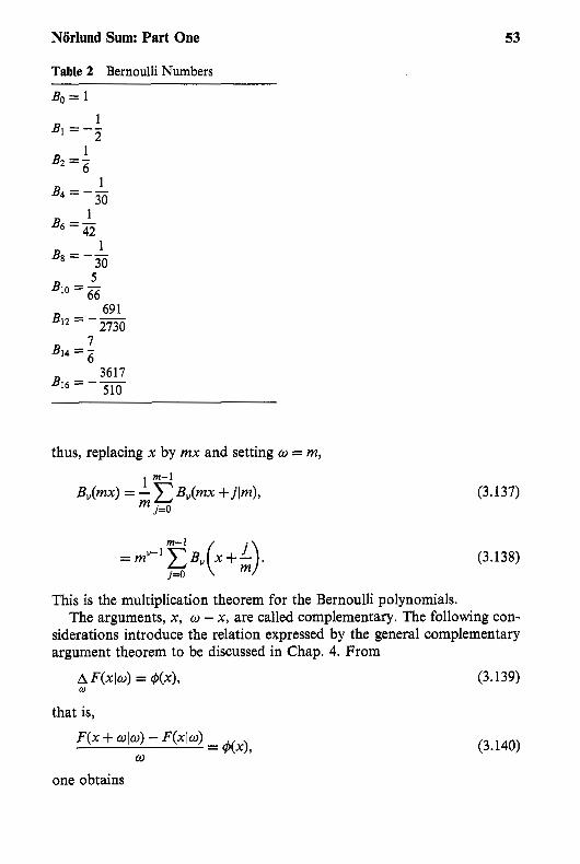
Norlund Sum: Part One 53
Table 2 Bernoulli Numbers
Bo = 1
5 B10 = -
66 69 1 2730
B12 - -
thus, replacing x by mx and setting o = m,
(3.137)
(3.138)
This is the multiplication theorem for the Bernoulli polynomials. The arguments, x, o - x, are called complementary. The following con-
siderations introduce the relation expressed by the general complementary argument theorem to be discussed in Chap. 4. From
that is,
one obtains
(3.140)

54 Chapter 3
F(xl - W ) - F(x - W1 - = $(x) W
(3.141)
on replacing W by -W and assuming that the principal sum F(xl - W ) exists. But (3.141) implies
A F(x - - W ) = $(x) (3.142) a,
from which one has F(x - W1 - W ) = F(xlw) + p ( x ) (3.143)
in which p(x ) is a periodic of period W. This is called the complementary argument formula. The character of $(x) determines p(x) .
For application of these ideas to &(x), observe that (- 1)”+’Bv+1(l - x ) satisfies
A(-l)”+’Bvt1(l - X ) = (U + l ) ~ ” , (3.144)
which is verified directly; hence,
Butl(x) = ~ - l ) v + l ~ u + l ( l - x ) + P ( X ) . (3.145) Since &(x) is a polynomial, p(x ) can only be a constant. Thus, differentia- tion yields the result
B,(x) = (-1)”Bv(l - x), (3.146)
which is the complementary argument theorem for the Bernoulli polyno- mials. It is now seen that B2,,(x) is symmetric about x = 4, and B2H1(4) = 0.
From (3.127), one has
B”(1) = B,, U L 2, (3.147) and, from (3.146),
B, = (-l)”B,(l) = (-l)”&, U 2 2, (3.148)
hence &”+l = 0, U L 1 . (3.149)
Further properties of the numbers B, follow from the generating function for &(x), to be derived now. Let
(3.150)
(3.151)
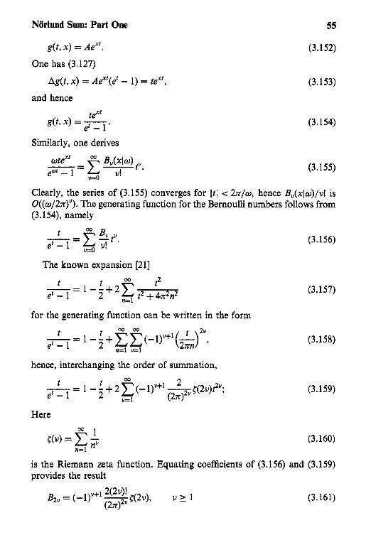
Norlund Sum: Part One 55
g(t, x ) = AeXfI
One has (3.127)
Ag(t, x ) = Aexr(ef - 1) = lexr,
and hence
Similarly, one derives
UteXt B (xlw) - = c v tu. ew‘ - 1 v=o V!
(3.152)
(3.153)
(3.154)
(3.155)
Clearly, the series of (3.155) converges for It1 < 2n/w, hence B,(xlw)/u! is 0 ( ( ~ / 2 n ) ~ ) . The generating function for the Bernoulli numbers follows from (3.154), namely
t w
u=o
The known expansion [21]
t t w t2 -= 1 -z+2c er - 1 t2 + 4n2n2 n=l
for the generating function can be written in the form
t t t ”
er - 1 n=l u=l hence, interchanging the order of summation,
t t w 2 ”
e‘ - 1 2 - l - - + 2 c (- 1)V+’ - <(2v)t2”; u=l (2n)2u
Here
(3.156)
(3.157)
(3.158)
(3.159)
(3.160)
is the Riemann zeta function. Equating coefficients of (3.156) and (3.159) provides the result
= (-l)”+l-<(2U), U 2 1 2(2u)! (2n)2”
(3.161)
.. . . , , _ , . . , , , . . . I _/..,,,,.,.,./ :,>* ..,../,. . . . . . . . . .

56 Chapter 3
from which one has
(-1)”” B2” > 0. (3.162)
Since ((m) = 1, (3.161) gives the asymptotic behavior of B2” for U large. In view of the recursion (3.131), the Bernoulli numbers may be assumed com- pletely known, hence (3.161) in the form
(3.163)
(3.164)
12. COMPUTATIONAL FORMULAE
The material of this section is concerned with various practical expansions and with the means of numerical evaluation. These expansions are derived in a formal manner with no attention given to their range of validity. This may seem somewhat unusual but, in numerical practice, one usually cannot ascertain a priori the conditions of validity; however, pointwise error esti- mates will be derived in terms of derivatives.
The first expansion to be considered is Norlund’s version of the Euler- Maclaurin formula to be studied in Chap. 4. Let
then
(3.165)
(3.166)
Substituting the Taylor expansion for #(x + z) in powers of z into (3.166), one has

Norlund Sum: Part One
Since
one obtains
and hence, x+hw 5 4(z) A z = [ #(z)dz + c TBu(h)q5(’”1)(x).
wv 0 V. v= 1
The special case h = 0 is of particular importance, thus
g #(z) A z = [ 4(z) dz + c O3 -Bu4(u-1)(x). ow 0 V!
U= 1
57
(3.167)
(3.168)
(3.169)
(3.170)
(3.171)
This expansion is asymptotic for x -P CO and also for o + O+; it is not usually convergent. It provides, however, excellent approximations. It is, of course, exact when @(x) is a polynomial. Let
and define Rm(xlo) by X
S 4(z) A z = Qm(XlW> + Rm(XIw)* W
Then, by (3.171)) one may take
(3.173)
(3.174)
in which m may be increased to obtain the first nonvanishing term. An exact representation of Rm(xlo) is given in Chap. 4. An example of (3.173) and (3.174) is
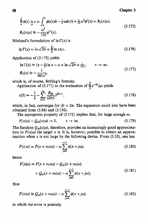
58
+(z) A z = +(z) dz - $o&(x) + #jwZ+'(x) + & ( X ~ W ) , W
W 4
R z ( x 1 w ) E --+"'(x). 720
Norlund's formulation of In r(x) is
In r(x) = In 6 + 8 In zAz.
Application of (3.175) yields
l n r ( x ) ~ ( x - ~ ) l n x - x + I n ~ + ~ , x + c q 1
& ( X ) G - - 360x3 '
which is, of course, Stirling's formula. 0 Application of (3.171) to the evaluation of f e-"Az yields
1 h(S) = - - -
k=l
Chapter 3
(3.175)
(3.176)
(3.177)
(3.178)
which, in fact, converges for IS1 < 2rc. The expansion could also have been obtained from (3.88) and (3.156).
The asymptotic property of (3.171) implies that, for large enough m, F(x~w) - Q , ( x ~ w ) + 0 , X + 00. (3.179)
The function Q m ( x l w ) , therefore, provides an increasingly good approxima- tion to F(xlo) the larger x is. It is, however, possible to obtain an approx- imation when x is not large by the following device. From (3.33)' one has
r-l F ( X l W ) = F(x + rwlw) - W x +(x + j W ) ,
/=o
hence
F ( x ~ w ) = F(x + ~ w I w ) - Qm(x + ~ w I w ) r- 1 + Q m ( x + ~ w I w ) - W C +(x + j ~ ) ; /=o
thus r-l
F ( x ~ w ) G Q m ( X + ~ w I w ) - W C +(X + j ~ ) j=O
in which the error is precisely
(3.180)
(3.181)
(3.182)

Norlund Sum: Part One 59
F(x + rwlw) - Q,(x + r ~ l ~ ) .
In view of (3.179), one also has
(3.183)
r- 1 Q,(X + rwlw) - WC 4(x + j w ) 1 (3.184)
r+ 00 j=O
or, equivalently, Do
F(xlw) = Q,(xl@) + W C [A Q& +j4~) - + j ~ ) l - (3.185)
As an illustration of (3.182), the computation of In r(x) to an accuracy
W j=O
better than lo-' uniformly for x 2 1 may be accomplished by choosing
Qz(x)=(x-h)lnx-x+ln&+& (3.186)
and approximating by
Define
(3.187)
(3.188)
which is the expression used in the lower bound theorem; then L(x10) pro- vides an excellent approximation even when summing a function that is not completely monotone or even a Laplace transform. Let R(xlw) designate the error, so that one has
X
S 4(z) A z = L(xlw) + R(xlw). (3.189) W
Then an estimate for R(xlo) may be obtained using (3.171) and (3.178), and the following expansion is obtained,
1 1 L ( X l W ) = - -@(x) + -u2#'(x) - - 1 4 4'W3
2 12 720 4(x)' W - + * * * . (3.190)
Use of (3.171) yields the expansion 1 1 1 6 4(z) A z = - -@(x) + - W 2 4 ' ( X ) - - W44"'(x) + - , (3.191)
X 2 12 720 w
hence

60 Chapter 3
An interesting implication of (3.192) is the inequality
(3.192)
(3.193)
valid for completely monotone functions with equality occurring for 4(x) = e-”. Generally, however, the sign of R(xlo) depends on x and W .
The numerical computation of Qz(xlw>, &(xlw), L(xlw), and R(xlw) may be accurately and conveniently accomplished by use of numerical differen- tiation. Let
ah = Eh12 - E-h/2 (3.194)
then the following formulae are suggested:
1 f$”’(x) E g S&X).
(3.195)
The integral in the expression for Q,(x~w) may be evaluated by use of standard quadrature rules such as the Simpson or Gauss-Legendre rules [22]. The Gauss-Legendre rules are particularly efficient when applied to sufficiently smooth functions; an n-point rule has degree of precision 2n - 1. Writing the rule in the form
(3.196)
then the nodal points, z t ) , and weights, A t ) , are symmetric with respect to z = 0; that is,
A t ) - - An-k+l 9 zt ’ = -zn-k+l(n). (3.197) Thus, it is sufficient to tabulate only for 0 5 z t ) 5 1. Table 3 lists the values for n = 10.
The numerical evaluation of S:f(z) A z directly from (3.90) is readily effected by use of the Gauss-Laguerre qfiadrature rule. This rule takes the form
(3.198)
and also has degree of precision 2n - 1. Writing (3.90) in the form

Norlund Sum: Part One 61
Table 3 Data for Gauss-Legendre Rule
,97390 65285 ,06667 13443 ,86506 33667 .l4945 13492 ,67940 95683 ,21908 63625 ,43339 53941 ,26926 67193 ,14887 43390 ,29552 42247
(3.199)
one may identify (3.199) with (3.198). Table 4 provides a list of tfo) and
The negative numbers in parentheses indicate the power of 10 by which the A:') are to be multiplied.
A quadrature evaluation proceeding by successive derivatives, such as (3.170), is said to be of Euler's type. One may also obtain evaluations in terms of successive differences, in which case they are called Laplace's type. An expansion analogous to (3.170) will now be derived.
AfO)
From (1.8), one has
hence, using (3.166),
Table 4 Data for Gauss-Laguerre Rule
,13779 34705 ,72945 45495 1.80834 29017 3.40143 36979 5.55249 61401 8.33015 27468 11.84378 58379 16.27925 783 13 21.99658 58120 29.92069 70123
,30844 11158 ,401 11 99292 .21806 82876 ,62087 45610 (-1) .95015 16975 (-2) .75300 83886 (-3) .28259 23350 (-4) ,42493 13985 (-6) .l8395 64824 (-8) .99118 27220 (-12)
(3.200)
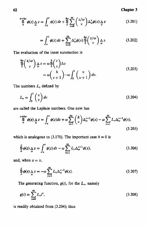
62
x+ho 5 #(z) A z = 1’ #(z) dz + $j c (‘r) A:#@) A z hw W
a u=o W W
The evaluation of the inner summation is
The numbers L , defined by
L u = I ’ ( ; ) d V
Chapter 3
(3.201)
(3.202)
(3.203)
(3.204)
are called the Laplace numbers. One now has
x+ho W
U= 1 u=l 5 #(z) A W z = 1’ #(z)dz + W 2 (S> A;-’#(x) - W c L,A:”’#(x),
a
(3.205)
which is analogous to (3.170). The important case h = 0 is
00 4 #(z) A z = L x # ( z ) dz - W c L,A:-’#(x), (3.206) W u=l
and, when a = x,
The generating function, g(t) , for the L,,, namely
(3.207)
(3.208)
is readily obtained from (3.204); thus

Norlund Sum: Part One 63
s(t> = v=o
l = l (1 + t)"dv (3.209)
t " -
ln(1 + t ) '
which converges for I tl 1 . The corresponding recurrence relation is
1 1 1 (-l)"+' L, = 5 L"-1 - - L"-2 + ;r LP" - - 3 +-
v + l LO (3.210)
Table 5 lists the first few numbers.
kind; thus from (1.34), The Laplace numbers may be written in terms of Stirling numbers of first
( ; )=$kSi . ' , hence, using (3.204),
j=1
Table 5 Laplace Numbers
Lo = 1
1 L, =- 2
1 L2 =-- 12
1 L3 =- 24
19 L4 =-- 720
863 L6 =-- 60480
275 L, = - 24 192 33953 L8 = -~
3628800 5728 1
7257000
'' - -479001600
Lg =-
3250433 L -
, , .. , , , , . , ./ , .. . _ , , ., . .. .... .. ,. ,̂ .. . , . , . . , , ... . , . . ,..,. . . I ...I_ "..l ..l/.. ....... . , , ,I. . . , . ._. . . . . .

64 Chapter 3
(3.212)
The mean value theorem applied to (3.204) yields
L,= G), o < e < 1 , (3.213)
which has a fixed sign for any choice of 0 E (0, l), hence
(-1)”+’L, 2 0, W 2 1 . (3.214)
Pointwise error estimates for the Laplace expansion may be obtained simply by considering the next term. Consider the expansion to A;#(x) and define R(xlw) by
H(xlo) = - ~ w # ( x ) + &~A,#(x) - &wA~J#(x) + R(xlo); (3.215)
(3.216)
(3.217)
(3.218)
so that one may use
R(xlo) E &04#”’(x) (3.219)
if the derivative form is more convenient. Error estimates obtained in this manner presume, of course, convergent or asymptotic behavior of the infi- nite expansion for the function represented so that the basic error is due to truncation. When the infinite integral and series both converge, then (3.207) becomes the classical Gregory-Laplace quadrature formula [20]
(3.220) - 1 @(x) + h wA,#(x) - h wA;#(x) + ,
This formula is very useful when numerically solving integral or differential equations producing the values #(x + j w ) , j 2 0 and the value of the integral is required. If #(x +jo) has been computed for sufficiently large values of j
Norlund Sum: Part One 65
so that the truncation error of the infinite sum is negligible, then the correc- tion terms can provide high accuracy.
Consider the following example. The Volterra integral equation
40.1) = .3e-Y + .3 4(t)e”’-Ydt LY (3.221)
arose in an M/G/l queueing problem with reneging (see Chap. 5); it is required to compute $0.) dy.The exact solution is known for this exam- ple, namely
40.1 = ,3e-y+.6-.6e-Y’z 9 LW q!~(y)dy = ( 1 5 ~ ~ - 24)/9 = ,370198,
(3.222)
hence a control is available for the quadrature method of (3.220). The choice W = . l was made and a numerical solution of (3.221) was constructed. The values obtained are
150 . l C4(.lj) = ,385373,
j=O
4(0) = .300000, A&(O) = -.020488, A$$(O) = .001028, A:#(O) = -.000002.
Use of (3.220) up to the term A;$(O) yields
LW r$b)dy = ,370198,
(3.223)
(3.224)
which is seen to be correct to the last figure. The error estimate of (3.216) yields
R(Ol.1) = -5.28*10-’. (3.225)
The evaluation of
(3.226)
in which p(z) is a given weight function is often useful. One may write 0
H,(x~w) = f p(x + z)#(x + 2) A z , (3.227) W
hence, using (3.200),

66
!J=o
with
0 A,,(xlw) = f p(x + Z)
The important special case p(z) = e-" yields*
Chapter 3
(3.228)
(3.229)
0
0 (3.230) (9 Az* A,,(x, S ~ O ) = ON-" s e+"
Define A,@) by
0
0 A&) = w S e-@'(;) Az; (3.231)
then comparison of (3.23 1) with (3.230) shows that
thus only A&) need be investigated. The generating function for A,(o) , namely
(3.233)
is 0
0 g(t) = wSe-O'(l + t)"Az. (3.234)
This can be written in the forms
g(t) = wA(w - In( 1 + t)) , (3.235)
(3.236)
The first few coefficients A,(o),may be obtained by direct expansion of g(t); Table 6 provides a listing.
*It was pointed out to the author that F. D. Burgoyne in 1963 had obtained a similar quadrature formula for the evaluation of an integral.

Norlund Sum: Part One 67
Table 6 Coefficients for Exponential Weight
In practice, one uses (3.229) for p(z) = e-" in the form
(3.237)
R(xlw)Z ~e-"rA4(6o)A~r$(x). S
The error, R(xlw), is estimated by the next term of the expansion. Values of W smaller than .01 should not be used in the formulae of Table 6 because of severe loss of numerical accuracy. It will be proved in Chap. 5 that
(-l)"+'Au(W) > 0, W > 0, U 2 1; (3.238)
a consequence of the proof will be an expansion for A&) permitting accu- rate computation when W is small.
An example is given by the evaluation of 1 S - A z . 1 1 + z . 2
(3.239)
Here p(x) = e-' so that (3.237) will be used. One has from (3.234)
Ao(.2) = -.103331, A1(.2) = ,016633, A2(.2) = -.008151, (3.240) A3(.2) = .005103, A4(.2) = -.003600.
Thus, for the Norlund sum, one gets
(3.241)
68 Chapter 3
Table 7 Coefficients for p(z) = z
C,(XlW) = - - OX 12 '
with
R(ll.2) = -6.7*1OW7. (3.242)
The weight function p(z) = z is important in applications such as com- puting means; it may be derived from p(z) = e-" by differentiation with respect to S at S = 0. Define C , ( X ~ W ) and g(t) by
(3.243)
then g(t) is
g(t) = wxh(- In(l+ t ) ) - w2h'(-- In(l+ t)). (3.244)
The determination of C,(xlw) is simply accomplished by use of (3.178) and the expansion of ln(1 + t ) in powers of t. The first few coefficients are given in Table 7.
PROBLEMS
Show
Show x 2 1 1 S- Az=ln3---- 1 z(z + 2) x x + l '

Norlund Sum: Part One 69
3. Show
z 3 + z + l ? (z + l)(z + 2)(z + 3)
Az=x-6$(x+1)+201n2
1 29 4 20 29 1 ”“ h---+-
2 2 3 x + 1 2 (x+ l ) (x+2) ’
Hint: Consider the Newton expansion in forward differences of z3 + z + 1 about z = -3.
4. Show X
scosmzAz=- W sin m(x - f W) sin ma
a W 2 sin(mw/2) --
m 5 . Show
X W cos m(x - f W) cos ma SsinmzAz= -- a W 2 sin(mo/2) +-. m
6. Show
7. Show that the repeated sum F ~ ( x ~ w ) for vx”” (U 2 1) on the range (0, x) is
V N x l 4 = (x - o)B,(xlw) - V+lB,+l(XlW).
8. Obtain the following expansion for the @-function: cc (-l)’u!Lu+l
+(x) = 1nx - C x ( x + 1) * * (x + v)’ u=o
9. Obtain the approximation ( p > 0) cc
j=O
10. Obtain the following asymptotic formulae: x 1 1 1 S- A Z - tan” x - -- oz2+1 2x2+ 1’
x ” , 00,

70
11.
12.
13,
14,
15,
16.
Chapter 3
Let f ( z ) be completely monotone for z 2 0 and (IY L 0 and then show
Show
00
A(S) = - x(--l)”L,(l - e-Sy-1, v= 1
Show
Show that the coefficients, C,(xlw), in (3.243) can be expressed in the form
Define g(t) by
show
1 1 &) = - - - Ssms S - 1 ’
Define the Binet function, ~ ( x ) , by
l n r ( x ) = ( x - { ) l n x - x + I n ~ + W ( x )
and 4 0 ) by
q5(x)=(x+{)AInx- 1,
and then show

Norlund Sum: Part One 71
P(X) = - - S #(z)Az, l X 4 0
17. Obtain the expansion (S L 0)
18. It is expected that L(xlw) (3.188) will constitute an exceptionally good approximation for functions #(x) satisfying
Show that
K[cosh(cx + K[sinh(cx + d)I2l3,
K, c, d constants, are solutions.
19 Obtain the following expansion for the Riemann zeta function: m
20. Show 1 m < 7 - - W
21. Solve u(x + 1) - #(x) = xsinx.
22. Define #"(x) (U = 0, 1, 2, . . .) by
and then show

72 Chapter 3
(1 + ty- = c 4u(x)tu. ln(1 + t )
t u=o
23. Let (see Prob. 22) W
show
24.
25.
Obtain the following numerical results for yo, y1 of Prob. 19:
1 1 yo = - S - AZ = ,57722,
1 z
y1 = S - AZ = ,07282. 1 lnz 1 z
Hint: The use of L(xlw) (3.188) or of (3.207) serves as an excellent means of computation; (3.207) is often used to tenth differences. These formulae are readily coded for use on a desktop computer. Because many functions have the property that high-order differences at a point x are small when x is large, high accuracy may be achieved by computing
Sf (z)Az
for large x and then using the following identity obtained from (3.12) and (3.33):
The integral may be evaluated by a quadrature rule such as the Gauss- Legendre rule (3.196). Simpson’s rule for the infinite interval may be written in the form

Norlund Sum: Part One 73
26.
27.
28.
29.
30.
Jdm 4(t) dt = ;[+(O) + 44(w) + 24(2w) + 4 4 ( 3 ~ ) + a ] + R(@);
show
Define Rf by
then show
Rf = - c ~ ( 2 ~ - ” - l)BuCf(’”’)(a) - f(!”’)(b)), 1 O0 hu 3 U. u=4
h4 h6 2880 6048
Rf CY - (f”’(a) - f’”(b)) - - (f”(a> -f”J(b)).
Show
O0 1 y - h(e0 - 1 ) 3 5 c=- W + - + - W , 4 144 W + O + . j= 1
Show
Show (a > 0)
Obtain the following numerical values:

74 Chapter 3
31. Let
Q ( X ) = 2 , h - 2 h ( l + ,h),
then show
0 1 S - AZ = -.646439, o l + & n- 1 1 1 1 Q(n) + .646439 - -- n + m.
2 1 + @ j=O
32. Show
33. The Euler constant, y($lw), of a function 4 relative to span W . is defined by
Show that the Mellin transform with respect to W is
34. Show
if and only if (n+l)o
lim S +(z) A z = 0;
in particular, this condition is met if $(z) is a Laplace transform.
n-*w (n+l)w W

4 Norlund Sum: Part Two
1. INTRODUCTION
The Norlund principal sum will be further developed. The Norlund form of the Euler-Maclaurin expansion (3.70) will be rederived in a rigorous fashion and trigonometric developments for the sum will also be obtained. A special class of linear transformations will be studied whose domain is the class of entire functions of exponential type. Application of these transformations to the solution of certain functional equations will be made.
The subset of entire functions for which various expansions converge uniformly in the complex plane will be determined. These expansions include the Newton forward difference formula and the Euler-Maclaurin formula. Application is further made to the extension of the Norlund sum to complex values of x, h, U. This extension finally allows a version of the complementary argument theorem to be proved.
2. THE EULER-MACLAURIN EXPANSION
The periodic Bernoullian functions, &,(x), are defined by
&(x) = &(x), 0 5 x < 1, &(x + 1) = &(x), vx.
(4.1)
75

76 Chapter 4
Since &(l) = B,(O), v > 1 , the functions &(x) are continuous, and from (3.127),
DB,(x) = vBu-l(x), v > 1 . ( 4 4
Thus &,(x) has continuous derivatives up to order v - 2. The function D""B,(x) is discontinuous at the integers, x = 0, f l , f 2 , . . . ; this follows from the discontinuous character of &(x); thus
B ~ ( x ) = x - + , O < x < l , &(O+) = - 2 , &(O-) = 4.
1
Consider the summation formula, (3.170), applied tOA $(x) W
x+ho S A #(Z) A z = +(X + h@) - - a m W W
A 4(z) dz + c 7 &(h) A &"'(x) O0 WV
V . v= 1 W
Thus
#(x + hw) = - c#@) dz + c 7 B v ( h ) A &"'(x). 6'" O0 0,
, W V . U= 1 W
(4.5)
Since (3.170) is exact for polynomials, so is (4.5). It is the present object to generalize (4.5) to apply to a wider class of functions. For this purpose, let @(")(x) exist and be continuous and let
Successive integration by parts yields
Taking into account the jump discontinuity of &(h - z) at z = h, one has
R1 = -(h - $ ) 4 ( ~ ) + (h - &(X + W ) 1 FX+O
- @(z) dz + $(x + hw).
Hence, finally, the usual form of the Euler-Maclaurin formula:

Norlund Sum: Part Two 77
#(x + hw) = !. #(z) dz + c -&(h) A &“-”(x) + R wv U! 0 w m . (4.9)
v= 1
A simple application of (4.9) is to $(x) = ex; then
(4.10)
Since, for 101 .c 2n) limm-+oo R,,, = 0, one has again (3.155), the generating function of the Bernoulli polynomials, namely
(4.1 1)
Consider now @(x) = cos x , h = 1, x = - 4 2 , then, after some manipulation,
O w m -Cot- = C ( - 1 ) v ~ B 2 v
w2” 2 2 v=O (4.12)
(- y w 2 * + 2 1 - 2 sinw/2 (2m + l)! 1 B2rn+1(Z) sin((z - $)U) dz.
(4.13)
3. EXISTENCE OF THE PRINCIPAL SUM
The Norlund theory [ 171 will be presented to establish the form of the Euler- Maclaurin expansion given in (3.170) and to provide conditions ensuring the existence of the principal sum. The following conditions will be imposed on
1. For some order m, #(“)(x) exists and is continuous for x 5 b, also
2. The integral
#(x) :
pqm) = 0.
loo B,,,(-z)&’)(x + wz) dz (4.14)
is uniformly convergent for b I x 5 B in which B may be arbitrarily large,
Use of I’Hbpital’s rule and condition (1) implies

78
+'"-'"'(x) limx+w =O, v = O , l , . . . , m .
X"
Condition (2) is implied by 3. The sum
Chapter 4
(4.15)
(4.16)
is uniformly convergent for b 5 x 5 B. To see this, consider
(4.17)
Thus the uniform convergence of the series of condition (3) implies condition (2).
It may be observed that both conditions (1) and (2) are met if, for some m, +(")(x) exists and is continuous for x 2 b and if also for some fixed E > 0, one has
(4.18)
In the Euler-Maclaurin expansion of (4.9), namely
the values x , x + W , , (n - 1)w are substituted in succession and the resulting equations are added; also, the function +(x) is replaced by (A > 0) and lax e-*'+(z) dz is added to both sides. The resulting equation is

Norlund Sum: Part Two 79
(4.20)
in which D refers to differentiation with respect to x. It will be assumed that a z b , x ? b . Set
~ ( x l w ; A ) = 5 e-AZ#(z) A z (4.21)
and let n --f 00 in (4.20); then, using (4.19, the left-hand side of (4.20) exists and, observing that the limit of the third term on the right-hand side of (4.20) is zero, one has
0
(4.22)
The investigation will proceed by examining the limit h + O+ of the remainder term of (4.22). Using (1.1 lo), one has
~ " [ e - ~ " q + ( x ) l = - A ) ~ # ( X ) , (4.23)
hence integrals of the form
must be studied. It will now be shown that
lim I, = 0, v > 0. A+O+
(4.24)
(4.25)
Integration by parts will be applied to (4.24); accordingly, introducing the function

80 Chapter 4
q 1 ( z , h) = LW e-*W'&(h - t ) dt,
one obtains
(4.26)
(4.27)
The behavior of the function q1(z, h) for h + O+ is obtained as follows:
ql(z, 1.1 = e-hor e-hwt&(h - z - t ) dt
(4.28)
Integration by parts applied to the last integral in (4.28) yields
(4.29)
and, hence,
(4.30)
It now follows that there exists a constant c for which
l+l(z, 9 5 Ce-*wr (4.31)
for all h > 0 and arbitrary z. The first term of I, clearly vanishes for h + O+ because lim g1(O) exists
while the limit of the second term is zero in view of (4.15) and (4.31), hence (4.25) has been proved. For the integral
*+O+
Io = LW e-*(x+Wz)j m (h - z)~(")(x + wz) dz,
integration by parts will again be used. Set
(4.32)

Norlund Sum: Part Two 81
(4.33)
then
Because of condition (2), the limit of the second term is zero, hence
lim Io = phZ(0) = - z)+(")(x + wz) dz. (4.35) I+O+
One now finally has
+$Lw &(h - z)r$")(x + wz) dz, 0 5 h 5 1,
(4.36)
Since all limits are uniform for b 5 x 5 B, F(x + hwlw) is continuous for x L: b. The expansion (3.170) is now made precise by (4.36), and the existence of the principal sum has been established under conditions (l), (2) or (l), (3).
The differentiation formula of (3.45) may be derived from (4.36). Assuming conditions (l), (3), F(x + hwlw) may be written in the form
F(x + hwlw) = [ 4(z) dz + c - Bu(h)&'")(x) m 0"
U! v= 1 W (4.37) + $1' &(h - Z) c #(")(X + wz + jw) dz. j=O
For m > 1, differentiation with respect to h yields
W
(m - l)! j=O
(4.38)
in which D indicates differentiation with respect to x. Letting h + 0 in (4.38) now gives

82 Chapter 4
(4.39)
Continuing the differentiation of (4.38) with respect to h up to order m, observing the jump at z = h of &(h - z), and letting h -+ 0 yield
W
D"F(x1w) = r$'""'(X) - W X +'"'(x +jo) j=O (4.40)
Hence
(4.41)
and, finally,
(4.42)
Thus the rincipal sum has continuous derivatives up to order m; further, since c$"- )(m) exists, one has, from (4.42),
lim D " F ( ~ I W ) = 4(m-1)(m), (4.43)
This property is characteristic of the principal solution of (3.1); any other solution differs from the principal solution by a periodic, p(x), hence lim,;,p(")(x) must be a constant that can only be zero. Thus, only the principal solution has the property expressed in (4.43).
The asymptotic properties of F(xlw) with respect to x + 00 and W + O+ asserted after (3.171) will now be established. As in (3.173), set
P x") W
R,(xlw) = - LW &,(-Z)~(")(X + wz) dz; m!
(4.44)
(4.45)
then
F ( x l ~ ) = Qm(XIW) + Rm(xla), (4.46) which is (4.36) for h = 0. Conditions (1) and (2) imply

Norlund Sum: Part Two 83
lim R,(xlw) = 0, (4.47) x-+ W
hence lim [F(xlw) - Qm(xlw)] = 0, (4.48)
X+oQ
which is (3.170).
imposed that To study the asymptotic character with respect to W , the condition is now
(4.49)
be convergent. This clearly implies condition (2). From (4.45), for some constant c,
IRm(xlw)l 5 cwm+* lt$(m)(x + wz)l dz 5 cum ioQ lqj(m)(z)l dz, (4.50) 0
hence Iw""R,(xlw)l is uniformly bounded in x and W . Also, from
R,-l(xlw) = - B W"
m! m (X) + Rm (XI W ) 9 (4.5 1)
one has
thus R,(xlw) = o(w"), m 2 1.
(4.52)
(4.53)
Defining Ro(xlw) = - ho$(x) + Rl(xlw), (4.54)
one has
and, hence,
W+O+ lim F(xlw) = la $(z)dz,
(4.55)
(4.56)
which reestablishes (3.20) under condition (4.49). . It is possible to obtain a very simple bound for R,(xlw) in (4.46) that is
often used in practice. For this purpose the following assumptions are made:
c#J(")(x) is continuous for x 2 b.
C qb(*")(x + j w ) is uniformly convergent for b 5 x 5 B (B arbitrary). j=o
W

a4 Chapter 4
lim 4(2m-1) (~) = 0.
~$(~")(x) does not change sign ( x 2 b).
Observing that j h ( - z ) = &(z), one may write
x") W
m-l w2u
v= 1 F(xlw) = [ 4 ( z ) d z - ;4(x) + ~ - B 2 , 4 ( 2 u - 1 ) ( ~ ) (2u)! + R2,,,, (4.57)
w2m+l W
Rzrn = - ( W ! 0
S ( j2 , ( z ) - B2m)4(2")(x + wz) dz. (4.58)
Thus:
Setting m = 2 in the multiplication theorem (3.138) yields
B " 2 (L) = (2lnU - l)&; (4.60)
hence, since the maximum of IB2,(z) - Bzm I on (0,l) is IBzm($) - Bzrn I = 2(1 - 2-2m)1B2m1, the Darboux mean value theorem applied to (4.59) yields
(4.61)
Thus, the error is smaller in absolute value than twice the next term of the summation in (4.58); this is characteristic of asymptotic expansions.
4. TRIGONOMETRIC EXPANSIONS
Trigonometric expansions for F(xlw) can be readily obtained whose coeffi- cients are simply expressed in terms of 4(x). These representations are some- times useful for direct numerical computation and usually provide ready means of truncation error estimation. The condition expressed in (4.49) will be assumed so that F(xlo) will possess a continuous first derivative. A Fourier series for F(xlw) will be constructed for x. < x < x,, + W , x . 2 b, of period w which, by the condition assumed, will be convergent [23].
Accordingly, set
(4.62)

Norlund Sum: Part Two 85
for which the Euler formulae for the coefficients are
(4.63)
2rcnx F(xlw)cos- dx, n 2 1, (4.64) W
2rcnx F(x1w) sin- dx, n 2 1 . W
(4.65)
The integral of (4.63) is recognized to be the span integral, (3.22), hence
a0 = 2 l 4(x) dx . X 0
(4.66)
For the integrals of (4.64) and (4.65), it will be convenient to combine them into a single integral, namely
a, + ib, = --lo F(xlw)e12nnx/o dx 2 xo+o
, n z l , (4.67)
in which i is the imaginary unit, Consider again the function
~ ( x l o ; A ) = 6 e-AZ#(z> A z , (4.68) 0
which is given by the uniformly convergent expansion
(4.69)
From (4.62), since F(x(o ; h ) + F(xJw) uniformly, one has
2 S"'" F(xIW)ei2nnx/w dx = lim 2 F(x1o; h)ei2nnx/w dx. (4.70) x0 h+O+ W
The representation (4.69) may now be substituted into (4.70); interchange of summation and integration is permissible by uniform convergence, hence one gets
The desired coefficients are now given by
(4.72)
86 Chapter 4
b, = - lim 2 1 e-Axq5(x) sin - dx. 2nnx A+O+ 0
(4.73)
The integrals of (4.72) and (4.73) are not usually convergent at h = 0; however, integration by parts will permit the limit to be evaluated in terms of convergent integrals. As an example, consider
X
F(x) S 22A2 = & ( X ) 0
for 0 x c 1; then
a0 = 0,
eqhx4x cos 2nnx dx,
e-hX4x sin 2nnx dx.
In this case the integrals are easily evaluated and one finds
4 2 n 2 - h2 1 a, = lim 4
b, = - lim 4
"
h+O+ (4x22132 + - nZn2 ' 4nnh
(4n2n2 + ~ 2 ) = '9
hence
As another example, consider
for 0 .c x < 1, then
a0 = 0,
a, = - lirn 2 LW cos 2nnx dx, A+O+
(4.74)
(4.75)
(4.76)
(4.77)
(4.78)
(4.79)
(4.80)
hence,
Norlund Sum: Part Two 87
26 4nznz + '
4nn 4 9 n 2 + d2 '
a, = -
b, = -
and W 26 cos 2nnx + 4nn sin 2nnx F(x) = - c
n=l 4n2n2 + sZ
(4.8 1)
(4.8 1 b)
The Fourier expansion of the $-function will now be obtained for x. x x0 + 1. Since
$(X) = S - Az, X 1
1 z
one has
a. = 2 r ' d z = 21nxo,
a, = - lim e-AX - cos 2nnx dx,
z w 2
A + O + L o X
b, = - lim e-AX 6 sin 2nnx dx. A+O+ jX0 X
Using the cosine and sine integrals defined by [24]
the formulae for a,, b, become a, = 2ci(2nnxo), b, = 2si(2nnxo);
thus the expansion for $(x) is
(4.82)
(4.83)
(4.84)
(4.85)
W
$(x) = In x. + 2 c (ci(2nnxo) cos 2nnx + si(2nnxo) sin 2nnx). (4.86)
When the function F(xlw) has jump discontinuities, the Fourier coeffi- cients are O ( l / n ) and the series is not rapidly convergent. To improve its use for numerical computation, the rate of convergence should be increased; this can be accomplished by removing the discontinuity. For this purpose define G(xl4 by
n=l
88
X
G(xlw) s(+(z) - ~ ( X O ) ) A W 2.
Then A G(xo(o) = 0, so no jump is present, and W
Chapter 4
(4.87)
~ ( x l w ) = ~ ( x l w ) + +(xo)(x - a - ;). (4.88)
The coefficients of G(xlw) are designated by ab, a;, b; and are given by
e-*X(+(x) - +(xo)) sin 2nnx dx.
The evaluation in terms of a0, an, bn is
ab = a. - 2+(x0)(x - a -;),
(4.89)
(4.90)
As an example, consider the function defined in (4.79) for which a = 0, x. = 0, +(xo) = 1 ; one has
ab = 0,
(4.9 1 )
the coefficients are now O ( l / n 2 ) so that the convergence has been much improved. The Fourier series for G(xlw) is
s2 G(x1w) = c -- 4n2 + s2 cos 2znx + n= 1 nn(4n2n2 + s2)
and
F ( x ~ u ) = G ( x ~ w ) + X - 4 I (4.93)
Another representation of F(xlo) will now be obtained from the Fourier series of (4.62) that is applicable for any x 2 b. If the formulae for the

Norlund Sum: Part Two 89
coefficients, (4.66), (4.72), and (4.73), are substituted into (4.62), the follow- ing equation is obtained:
(4.94) It is desired to set x = xo; however, at a point of discontinuity, the sum of the Fourier series equals the average of the left- and right-hand limits. Let S(x) denote the Fourier series for F(xlw), i.e., the right-hand side of (4.94), then
(4.95)
thus,
F(xol4 = S ( X 0 ) - +#4xo). (4.96) Now, setting x = xo, the required expansion is
W W
F ( X ~ W ) = #(z) dz - i&(x) - 2 c lim / + z) cos - dz 2mz a n= 1 A+O+ 0 W
(4.97) In this form, the infinite series is seen to express the difference F(xlw) and the asymptotic approximation provided by the first two terms.
5. A CLASS OF LINEAR TRANSFORMATIONS
A certain class of transformations will be studied whose properties readily enable one to discuss the convergence of finite difference expansions and to solve various forms of functional equations. Application will be made later in the chapter to the extension of the Norlund expansion of (4.36) into the complex plane. Norlund's own discussion of the extension of the Norlund sum into the complex plane is in Ref. 17. A deeper version of the material to be presented here may be found in Ref. 1.
A sequence of numbers (ak)r is of exponential order /.L if there exists some r > 0 for which
90 Chapter 4
and p = inf r. (4.99)
The linear vector space n(p) is the space of all functions #(z) of the complex variable z = x + iy ( x , y real) given by
(4.100)
in which the sequence is of exponential order not exceeding p. Let M(r) be the maximum modulus of #(z), that is,
max)#(z)I = M(r); (4.101) Izl=r
then, clearly, 4(z) is entire and
~ ( r ) = O(e(N+’)‘), E > 0. (4.102)
An entire function satisfying (4.102) is said to be of exponential type p; conversely, a function of exponential type t I p is in n(p). This follows from Cauchy’s inequality
l#(k)(0)l 5 k!M(r)r-k, r > 0. (4.103)
The choice r = R/(p + E ) and the use of Stirling’s formula for k! show that
I#(%)l = O((P + clk). (4.104)
The function @(() of the complex variable ( = 6 + iq ( 6 ’ 9 real) defined by
(4.105)
for [(l = p > p is called the associated function of #(z). One also refers to @(() as the Bore1 transform of #(z). One has the following relation connect- ing #(z) and @(().
Representation Theorem:
The path is a circle of radius p > p about the origin in the (-plane.
Proof. From (4.98), there is a K > 0 for which
lakl < K ( p + E ) k , E 0, (4.106)

Norlund Sum: Part Two
hence
Thus the series
is uniformly convergent on r. C
one now has
E < p - p .
(4.108)
91
(4.107)
lbserving that
(4.109)
Consider the analytic function
L(() = 2 a&'? k=O
(4.110)
(4.111)
in which it is assumed that the series converges for [(l = p0 > p so that L(() is analytic on and within l". The integral
defines the entire function O(z). The linear transformation T belongs to the class A ( p ) if and only if the domain of T is the space n(p) and the image of C$(z) E n(p) is e(z); that is,
T C $ ( ~ ) = q z ) . (4.113)
The function L(() is called the generating function of T .
Theorem: The transformation T transforms the space n(p) into itself, i.e., W ) E N P ) .
Proof. The series
converge absolutely and uniformly on r, hence
(4.114)

92 Chapter 4
(4.115)
The second summation in (4.1 15) is analytic on and within I', hence its contribution to e(z) in (4.112) is zero. Set
and
then 1 F
(4.116)
(4.1 17)
(4.1 18)
From (4.11 l), one has
lakl = w o k > , (4.1 19) hence
and, therefore,
B, = O((P + E l r > . Also, from (4.1 17) and (4.1 18), one has
thus O(z) E !&).
(4.12 1)
(4.122)
Uniqueness Theorem: The generating function L(<) uniquely determines its transformation; conversely, a given transformation uniquely determines its generating function
Norlund Sum: Part Two 93
Proof. T#(z) = 0 for all #(z) E Q(p) =$ L(() 0. To show this, consider z"/n! with the associated function (-"-l, From (4.11 1) and 4.1 17), the associated function of the image is
However, e(z) 0 ak = 0, 0 5 k 5 n.
Since n is arbitrary, it follows that
a k = 0 , k z 0
(4.123)
(4.124)
(4.125)
and hence L(() = 0. The first assertion of the theorem follows from (4.1 12). The converse statement follows from the next theorem.
Theorem: The function e'" is an eigenfunction of T whose eigenvalue is the corresponding generating function L(a); thus,
Tea" = L(a)e'". (4.126)
Proof. One has e'" E Q(lal), and the associated function is l/(( - a); thus,
(4.127)
in which the radius of is p. =- la/. The only singularity within is the simple pole at ( = a; hence, by residue theory,
Tea" = L(a)e". (4.128)
The sum Tl + T2 of two transformations in A ( p ) is defined by
v 1 + T2)#(z) = Tl W ) + T 2 W . (4.129)
The generating function of TI + T2 is L](() + L2(() because
(T1 + T2)ec" = T1e3" + T2ec2 = [Ll({) + L2(()]ec". (4.130)
Also TI T2 is defined by
TI T 2 m = Tl[T24(Z)l. (4.131)
Thus the generating function is Ll(()L2((). Clearly, TI + T2 = T2 + Tl,TlT2 = T2T1. (4.132)
The identity transformation I is defined by
= #(z) (4.133)
, . , . .,,, ..I , .." . " . . .

94 Chapter 4
and hence L({) 1. The transformation T-' with the property
TT-' = I (4.134) is called an inverse transformation of T .
Theorem: A transformation T E A ( p ) has a unique inverse T-' E A(p) if the generating function L({) of T is not singular at the origin and the distance of the nearest singularity from the origin is greater than p. The generating function of T" is then l/L({). Proof. Let the generating function be l(() , then
L(C)l(O = 1: (4.135) thus one must have
(4.136)
Since L(() is analytic in the neighborhood of the origin, the zeros of L({) are isolated. Also, it is assumed that L({) does not vanish at the origin; hence, L(() is analytic in a circle about the origin whose radius extends up to the zero of L({) nearest the origin. If the radius is greater than p, L({)-' uniquely determines a transformation of class A(p) . By (4.135), this trans- formation is inverse to T .
A sequence of transformations (T,)f' satisfying T, E A ( p ) for all n is said to converge to a transformation T E A(p) if
(4.137)
(4.138)
for all z and all #(z) E G@). The convergence is expressed symbolically by
n-+ 00 lim T, = T. (4.139)
Theorem: Let the generating functions of Tn, T E A ( p ) be L,({), L({) respectively, then
n-+ w lim T, = T =$ lim L,(() = L({)
n+ w
for all { within the path r. Proof. Let #(z) = e"", then

Norlund Sum: Part Two 95
T,,eaz = Ln(a)eaz, Tea' = L(cw)eaz, (4.140)
Since ea' never vanishes, the result follows.
Convergence Theorem: If the sequence (L,({))? of generating functions of T,, E A ( p ) converges uniformly on a circle that includes the circle I' to L((), then L({) is a generating function of a transformation T E A@); further, the sequence (T,,)? converges to T.
Proof. The limit of a uniformly convergent sequence of analytic functions is an analytic function, hence L({) is analytic on and within r and thus defines a transformation T E A(p) . Let e&), e(z) be the images under T,,, T respectively, of a +(z) E G?(p); then (representation theorem)
1 e (4 - e,(z) = G S, e5"Lt0 - J5,(0lW) 4 . (4.141)
By the uniform convergence of L,,(() to L((), one has
m;xlL(O - ~,({) l 5 8, n 5 W ) . (4.142)
(4.143)
(4.144)
lim e&) = O(z) (4.145) n-ma
for all z and +(z) E G?(p). In fact, (4.144) shows the convergence to be uniform in any compactum of the z-plane.
An immediate corollary is the following. cx)
Corollary: C &(C) converges uniformly to L(() on a circle including
implies C Tk = T. CO k=O
k=O For convenience, the generating functions for the commonly used opera-
tors are listed here. They may all be obtained from (4.128). Note that in

96 Chapter 4
these formulae w is an arbitrary complex number. The notation + will be used to relate an operator to its generating function.
eo( - 1 A+- , W 0
(4.146)
6. APPLICATIONS TO EXPANSIONS AND FUNCTIONAL EQUATIONS
The operational form of Newton's forward difference interpolation,
k=O W (4.147)
is
E" = (1 + W A)"'"; (4.148) W
in terms of generating functions, one has
(4.149)
in which the subscripts designate the corresponding operators. To obtain uniform convergence, one must have
(4.150)
which is satisfied by If1 In2/lwl; thus the following theorem.
Theorem: Newton's expansion is valid for all complex w # 0 and 4(z) E n(p) provided p < In 2/(wl. The convergence to 4(z + U) is uniform.
Norlund Sum: Part Two 97
As another application, consider the differential-difference equation #’(z) + U#(Z + W ) = q z ) . (4.151)
Let
= #’(z) + a#(z + U); (4.152) then
L(<) = < + ae’5. (4.153) The inverse transformation is given by
1 p j -. + @ew( ’ (4.154)
thus T” exists for c y in which y satisfies y + aewy = 0 (4.155)
and is the zero of L(<) nearest the origin. One may solve (4.151) for #(z) by use of the power series expansion
(4.156)
whose radius of convergence is ( y 1. The solution for #(z) has the form
(4.157) k=O
and the solution is valid for all O(z) E SZ(,u), p c (y I . The first four CO- efficients are
(4.158)
1 CO = -
a ’
a
a
An alternative form of solution may be obtained from the expansion
1 - - C O3 ( - I l k Fe - (k+1)N c + wew{ - &+l
(4.159) k=O

98 Chapter 4
This series converges for l J ' l < r 5 IyI where I is determined by re'W'r/lal = 1 . The solution is represented by the uniformly convergent series
m f(z) = &$P,, - (k + 1)w)
k=O (4.160)
for all O(z) E C@), p < Y.
Consider the first-order difference equation
A ~ ( Z I = (4.161) W
Since the generating function (eWc - l)/@ vanishes at J' = 0, no inverse exists for A; however, define T by
W
(4.162)
so that (4.161) takes the form
WYZ) = e(z), (4.163)
then 2"' is given by
provided l J ' l 2n/lwl. From (3.155), one has
hence the following theorem.
Theorem: The Euler-Maclaurin expansion
(4.164)
(4.165)
is the unique solution of (4.161) for all w # 0 and O(z) E Q(p) provided p 2n/(w( . The series converges uniformly and @(z) E n ( p ) . The expansion above may be compared to (4.5).

Norlund Sum: Part Two 99
7. APPLICATION TO THE NORLUND SUM
The Norlund sum
F(x + hwlw) = S +(z) x+hw
a (4.166)
and the corresponding expansion (4.36) will now be investigated by means of the transformation theory of the earlier section on linear transformations. Define T by
wehW( 1 L(() = - - - em( - 1 ( ’ (4.167)
which coincides with the eigenvalue belonging to et’ for
T4(x) = S 4(u) A U x+hw
(4.168) W
when c < 0 and z , h real. The function ,C(<) is meromorphic and the pole nearest the origin occurs at 27ri/w. Thus the expansion
(4.169)
(4.170)
This is consistent with the previous definitions, which are restricted to real z , O < h < l , w > O .
As an immediate application of (4.1 12), an integral representation for F(z + hwlw) will be obtained.
Theorem: One has
in which the radius, p, of I’ satisfies p < 27r/lwl.
Since it is a straightforward task to implement the numerical evaluation of a contour integral around a circle, the representation of the theorem is convenient for the numerical computation of F(z + hula).

100 Chapter 4 .-\
An application may now be made to the complementary argumencfor- mula of (3.143). In the formula
F(z - W1 - W ) = F ( Z l W ) (4.172)
replace z by z + 4 2 , then
(4.173)
which shows that the complementary argument formula is equivalent to the evenness of F(z + w/21w) as a function of W . Setting h = 1/2 in (4.170) and using (4.60), one obtains
which shows that F(z + 0/210) is, in fact, an even function of W .
Theorem: The complementary argument formula
F(z - W1 - W ) = F(zlw)
is valid for 4(z) E n(p), p 27r/101.
The expansion
(4.175)
obtained from (3.229) with p(z) = e-' and A,@) defined by (3.231) will now be investigated. One has
L(<) = A V = WA(W - WC), 0
0 0 (4.176)
hence, also,
L(<) = W ~ ( W - ln(1 + LAu)). (4.177)
As a function of ,CAu, the singularity occurs at -1; hence, one must have
le"(- 1 1 < 1. (4.178)
Theorem: The expansion (4.175) is valid for all complex W # 0 and $(z) E n(p) provided p In 2/14,

Norlund Sum: Part Two 101
8. BOUND, ERROR ESTIMATE, AND CONVOLUTION FORM
It is useful to have a bound on the magnitude of 8(z) as given in (4.1 12). One has immediately
p(z)l 5 W P l Z l m$(<)I m $ w l . (4.179)
The transformation Er given by the generating function W
Er(<) = c a k t , n L -1 (4.180)
is useful in error investigations. One may note that the associated function of a polynomial of degree not exceeding n is P(<) = C;=oak/<k+' and, hence, the product P(<)Er(<) is analytic within and on F; thus the image is identically zero. An estimate of the magnitude of 8(z) = Er($(z)) may now be obtained from (4.179); thus,
k=n+ 1
(4.18 1)
which follows because Er(( ) / f+ ' is analytic on and within P. A convolution integral representation of a transformation T will now be
obtained. Let c 1: 0 and p c c; let $(z) E S2(p), and S(u) be a summable function over (--oo,oo) satisfying S(u) = U(e-C'UI). Then one has the follow- ing theorem.
Theorem: The transformation W
T($(z)) = 8(z) = / $(z - u)S(u) du -W
belongs to A(p) , and the generating function L(<) of T is given by the bilateral Laplace transform of S(u), namely
L(<) = / e-cuS(u) du. W
-W
Proof. By the order condition on S&), the integral converges for all < in the strip --c c l j c c with l j = Re <. Thus the image of e(' exists and is given by
J -W J-W
this establishes the formula for L(<).

102 Chapter 4
An estimate for O(z) = Er(#@)) may also be obtained from the convolu- tion integral representation. Let S(u) be the integral kernel corresponding to Er(( ) / f+ ' ; then, since f+ '@({ ) is the associated function of #("+')(z), one has
(4.183)
Let S(u) vanish outside (a, b) with a, b not infinite; then the mean value theorem of the integral calculus may be applied to (4.183). Thus,
(4.184)
Theorem: Let S(u) vanish outside (a, b) and let S(u) 2 0 then
Proof. The mean value theorem may now be applied to the integral (4.183) for O(z) to obtain
J "00
Choosing #(z) = z"+'/(n + l)! yields
(4.185)
(4.186)
which completes the proof.
9. CONSIDERATION OF SOME INTEGRAL EQUATIONS
(4.187)
then

Norlund Sum: Part Two 103
(4.188)
Let L(0) # 0; then l/L(<) is analytic at the origin and T" exists uniquely and the solution of (4.187) for #(z) is
e(z) = T-~#(z) . (4.189)
The evaluation of T" may be carried out by a suitable expansion theorem for its generating function.
Example: To obtain #(z) from the integral transform
e,(z) = 1 e-iyU+(z + u) du, A > 0, nintegral. (4.190)
It may be noticed that O,,(O) are the Fourier coefficients of #(z) over the interval (-A/2, A/2), Defining T,+(z) = O,(z), the generating function is
-4
and, hence, the generating function of Ti1 is
1 (-l), A< - i2nn L , ( < ) - T sinh4A.r "
Consider
(4.191)
(4.192)
(4.193)
in which the singularity at the origin of (4.192) has been removed by multi- plication by <; the nearest singularity now occurs at < = i2nlA.Thus #'(z) E n(p) for p < 2n/A is uniquely determined by the series
For n = 0 set
then #(z) E Q(p) is uniquely determined for p < 2n/A by
(4.194)
(4.195)

104 Chapter 4
(4.196)
Certain types of integral equations of the second kind (inhomogeneous equations) may be solved by the present methods. Consider
W
in which S(u) = O(e-CIUI). Define the transformation T by W
T#(z) = O(z) + h S(u)#(z - U) du; L then the generating function L(() is
L(<) = 1 + h L, y F ' S ( u ) du. W
(4.197)
(4.198)
(4.199)
The function #(z) will be uniquely determined in some class Q(p) if L(0) # 0. It may happen that for special values of h, called eigenvalues, uniqueness is lost; this requires special consideration. Of course, one has
Example: To solve for #(z) : W
#(z) = O(z) - h e-"IU1#(z - U) du, 0 C a C C. J-W
One has
Thus
(4.200)
(4.201)
(4.202)
(4.203)
One has #(z) is uniquely determined for h # - 4 2 . When h = - a / 2 , then #"(z) is determined. Clearly

Norlund Sum: Part Two 105
(4.204) #”(z) = #(z) - a28(z).
10. BANDLIMITED FUNCTIONS
A class of functions of importance in communication theory consists of the functions representable in the form
(4.205)
in which g(u) is a real-valued function of bounded variation with variation VU(g). The quantity a is called the radian bandwidth and g(u) is called the spectrum of #(z). Clearly, #(z) is entire and belongs to n(a). To see this, one observes that
#‘k’(o) = p (iu)kdg(u)
I#(k’(O)I 5 “p Idg(u)I = V!,(g)ak.
-U (4.206)
-U
This class is designated B, (Bernstein class). Newton’s interpolation applied to #(z) requires the equidistant values # ( M ) , k = 0, 1,2, , . .. The quantity h =- 0 is the sampling interval and l / h is the sampling rate. One now has the interpolation formula
#(z) = 2 (zih)hk A #(O), ah < In 2. k=O h
(4.207)
A significant aspect of (4.207) is that #(z) is completely reconstructed for all z using only the sample values on the half-line.
PROBLEMS
1. Let 0 < alwl 2n and
f ( z ) = ~ g ( u ) c o s u z d u ;
then show

106 Chapter 4
2. Let 0 < olwl 2rc and
f(z) = l&) sin uz du;
then show
Consider the expansion
0 W 7 e-‘@(z) A z = C c,,(w)~(”)(o).
Show
W !J=o
C,(@) = - W u + l ~ ‘ ” ) ( W ) , U!
0 1 - e-0 ’
k=O
C&) = 1 - - W
C,(@) = 1 - 2 -we-.) 3 e-” + e-2W
Also show that the expansion is valid for +(z) E C@), p < 2rr/lwl - I Show
x 1 1 0 1 1 2nnz S- Az=tan- x - - - - cos - dz . 01+Z2W
Set
@(x) = - e-Ar cos - dt,
x(x) = - h e-*‘ sin- dt;
2mt
2mt X W W
W
then the Fourier coefficients a,,’b, in (4.72), (4.73) can be expressed in the form

Norlund Sum: Part Two 107
In particular, show that the necessary and sufficient condition for the absolute convergence of the Fourier series (4.62) is @(XO) = 0. Hint: use the formula
and the corresponding formula for ~ ( x ) ; also continue the integration by parts another step.
7. Show that in the asymptotic expansion (x +. m)
the error has the same sign as the next term and that its magnitude does not exceed that of the next term.
8. Show that (Newton's backward interpolation formula)
#(z+u) = c ( - l , " ( - y @ ) W k v O ( z ) W
k=O 0
converges for all #(z) E Q(p) with p < (ln2)/lol. 9. Show that
converges for all #(z) E Q(p) with p < (In2)/1ol. 10. Show that the root y of (4.156) is given by

108 Chapter 4
11. Discuss the following integral equations for @(z) given O(z) E Q(p):
P1
e(z) = lo eUr$(z + u) du,
#(z) = e(z) + h Lm e-""@(z - u) du,
@(z) = e(z) + S e-""@(z - u) A u.
a! > 0,
0
0 w
12. Let f ( z ) be completely monotone (z 2 0);. show 2
x - 0 S f ( z ) A z 2 - : f (x) + $(x), x 2 b > 0.
0
13. Letf(t) be convex on [0, 00), and define
14
15
The First-Order Difference E,quation
1. INTRODUCTION
This chapter discusses the first-order difference equation and certain func- tional equations resolvable with its help. The next section discusses the linear homogeneous equation; exact solutions are obtained and, also, a general approximation. Application is made to the gamma function.
Then the lipear inhomogeneous equation is studied and the general solu- tion is obtained. Application is made to the Erlang loss function of tele- traffic theory. The level crossing technique used in queueing theory is introduced and applied to the M/G/l queueing model with exponential reneging.
The method of Truesdell for the solution of certain classes of differential- difference equations is introduced. A GI/M/1 queueing model is chosen to exemplify the technique.
The following section is concerned with the computation of the deriva- tives of a function defined by a first-order difference equation. A simple approximation for the derivative is obtained that can also be extended to obtaining higher order derivatives. This is applied to the Erlang loss func- tion to obtain aB(x, a)/ax (see Prob. 3). These formulae have been applied to real-time teletraffic computations. An application is also made to the M/G/l queue with reneging discussed earlier to obtain an approximation for the mean work in the system.
109

110 Chapter 5
Functional equations and first-order nonlinear difference equations are then discussed. The infinitesimal generator of a difference equation is intro- duced. A special difference equation is solved that provides iterates of a bilinear form. The use of functional equations is illustrated by a queueing model with a recycling customer. Branching processes are defined and used to illustrate nonlinear difference equations. A standard birth-death model is solved.
Covered next is the solution of the first-order nonlinear equation. The U- operator method is introduced and a Newton expansion is given for the solution. The relation to semigroup theory is discussed. Acceleration of convergence of the Newton series is achieved by comparison with an invar- iant function; this is numerically illustrated. An expansion is obtained for the infinitesimal generator.
Critical points of a difference equation are then defined and classified and criteria are developed for their classification. After this, the construction of an approximation for the probability generating function of discrete branch- ing processes is presented.
The next two sections provide powerful means of approximating the solution of the difference equation when the span is small. First, a perturba- tion solution for Z(t ; zlh) is obtained in powers of the span. Second, the Haldane solution for the infinitesimal generator is presented. This, of course, allows the technique of differential equations to be used to approx- imate the solution of a given difference equation.
In the next-to-last section, a return is made to the problem of solution of functional equations. A general procedure is discussed and an example is given. The solution of the queueing model introduced earlier is completed.
The final section extends the U-operator method and Newton expansion to the solution of autonomous, simultaneous, first-order equations. The relation of the Lie-Grobner theory of differential equations is shown. Infinitesimal generators and characteristic functions are defined. Three examples are given. The first example illustrates the conversion of a non- autonomous system to autonomous form. The second example provides the background for the introduction of Euler summability in order to increase the range of applicability of the Newton expansion. The third example obtains an interpolation formula for the Erlang loss function that is much used. Finally, an approximation is obtained for the infinitesimal generators.
2. THE LINEAR HOMOGENEOUS EQUATION
The equation to be studied is

The First-Order Difference Equation 111
u(x + W) - a(x)u(x) = 0, W > 0.
An alternative form is 1
A In u(x) = -In a(x) ( 5 4
from which, if conditions 1 and 2 of Chap. 4 are satisfied by In a(x), one has 0 W
in which p(x) is an arbitrary periodic of period W. The required conditions are met if there is a c so that for some E > 0, m > 0
D" In a(x) = O(X-"~), x L c, b 2 c. (5.4)
Further, if the principal solution is required (4.43), then p(x) reduces to a constant.
The following example will illustrate the solution (5.3) and also the use of the multiplication formula (3.15). Consider
u(x + W ) - xu(x) = 0; (5 .5 )
then, from (5.3),
lnu(x) = c+-S lnzAz 1 X W O 0
in which c is an arbitrary constant. Norlund's definition of the generalized gamma function, r(xlw), is obtained by setting c = In m; hence,
One has r(xl1) = r(x) (3.176). The change of variable z = oy in (5.7) yields
r(xlW) = r(;>e X (x /w- 1) In o (5.9)
The multiplication formula, with W = 1, applied to the principal sum W In (xlw) - w ln yields
(5.10)
Since, from (5.8),
= In r(mx) - (mx - 1) In m, (5.1 1)
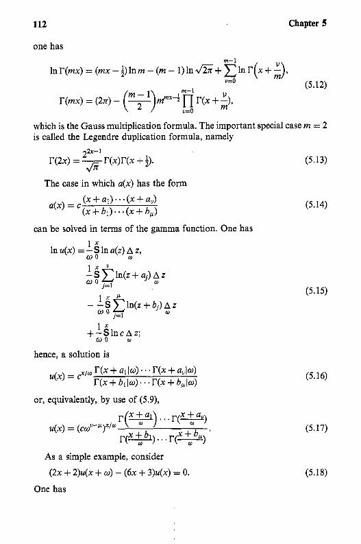
112 Chapter 5
one has
which is the Gauss multiplication formula. The important special case m = 2 is called the Legendre duplication formula, namely
The case in which a(x) has the form
can be solved in terms of the gamma function. One has
In u(x) = - S In a(z) A z, 1 X 0 0 W
- S C l n ( z + u j ) A z 1 x
- - S x h ( z + b j ) A z
+-SlncAz; W O W
0 O j=1
1 x
W O j=1
1 X
W
W
hence, a solution is
r(x + al I W ) r ( X + aUlw> r(x + bl IW) . r ( X + ~ , I w )
u(x) = c"/"
or, equivalently, by use of (5.9),
As a simple example, consider
( 2 ~ + ~ ) u ( x + W ) - ( 6 ~ + ~ ) u ( x ) = 0.
(5.13)
(5.14)
(5.15)
(5.16)
(5.17)
(5.18)
One has
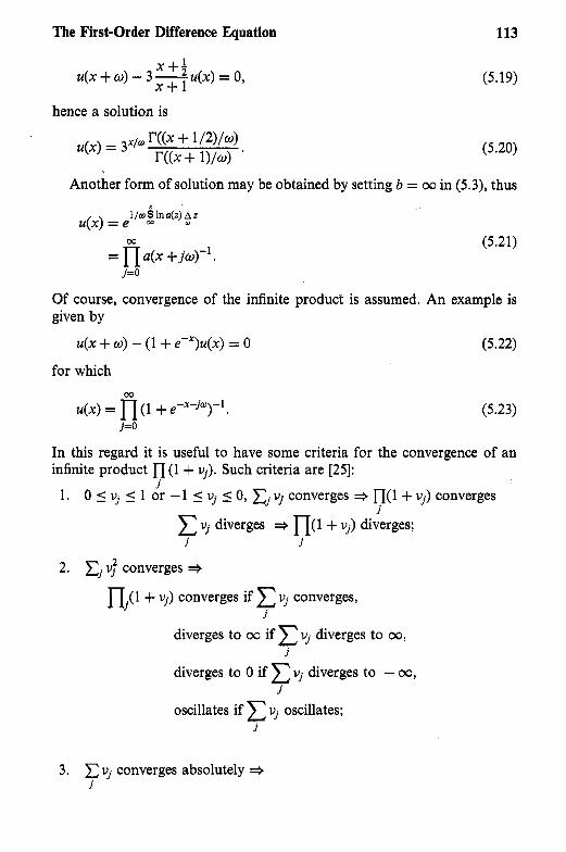
The First-Order Difference Equation
1 u ( x + W ) - 3 - x + u(x) = 0,
x + l hence a solution is
113
(5.19)
(5.20)
Another form of solution may be obtained by setting b = 00 in (5.3), thus
1 / U 2 In a(z) 4 z X '
u(x) = e W
= n a(x + j w p j=O
(5.21)
Of course, convergence of the infinite product is assumed. An example is given by
u(x + W ) - (1 + e+>u(x) = 0 (5.22)
for which
(5.23)
In this regard it is useful to have some criteria for the convergence of an infinite product (1 + vi). Such criteria are [25]:
1. 0 5 vj 5 1 or -1 5 vj 5 0, cj vj converges + n(l + vj) converges j
J c vj diverges + n(l + uj) diverges; j j
2. cj uj converges + n j ( l + uj> converges if C vj converges,
i
diverges to 00 if c vj diverges to 00, j
diverges to 0 if c vj diverges to - 00, j
3. C uj converges absolutely =+ j

114 Chapter 5
n( 1 + uj) converges absolutely. j
With respect to uniform convergence, the following theorem is useful:
Theorem: Let u j b ) be continuous for y E [a, b] for each j , and let 1 Vjb) I 1. vj 0, E [U, b]) with C uj convergent, then n ( l + Uj b)) is a continuous
function of y for y E [a, 4. i i
Application of this theorem to the solution in (5.23) shows u(x) to be a continuous function for all x .
The form of solution in (5.21) satisfies the boundary condition u(00) = 1 under uniform convergence. An approximation to this solution may be obtained by use of the Norlund expansion (3.171); thus,
In u(x) = - S In a(z) A z 1 x
W W 0
1X W O W W O
= -Sha (z )Az- - In a(z) dz
1 W a'(x) 2 12 a(x)
lna(z)dz--lna(x)+--+.--.
An approximation to u(x) is, accordingly,
W
u(x) 2: a(x)"/* exp [ - 1 In a(z) dz + - - W a'(x)
W , 12 a(x) 1 '
(5.24)
(5.25)
in which the error may be estimated from the next term of the expansion in (5.24), namely -(w3/720)D3lna(x). Since, for convergence of (5.21), one must have a ( m ) = 1, if also, a'(00) = 0, then the approximation satisfies the required boundary condition at x = 00.
For the example of (5.22), one has
1 u(x) N 4- (5.26)
The error estimate to be used in the exponent of (5.26) is (w3/720) ex(ex - l)/(ex + l)3. It may be observed that the approximation (5.25) is particularly useful when W is small because then the product (5.21) is slowly convergent.

The First-Order Difference Equation 115
3. THE INHOMOGENEOUS EQUATION
The complete equation of first order is
U ( X + W ) - U ( X ) U ( X ) = b(x), W > 0. (5.27)
The solution may be constructed from the solution, u(x), of the correspond- ing homogeneous equation
u(x + W ) - a(x)u(x) = 0 , (5.28)
which, from (5.3), may be taken to be
(5.29)
The summation without a lower limit expressed is here used as an indefinite summation symbol. Thus, let
u(x) = u(x)t(x); (5.30)
then substitution into (5.27), yields
b(x) A t(x) = W WU(X + W ) *
One now has
u(x) = u(x) [ p(x ) + - S - A z ] 1 X b(z) W u(z + W ) W
(5.31)
(5.32)
As in the case of the homogeneous equation, the principal solution is obtained by replacing the periodic, p(x), by a constant.
For many applications, a useful form of solution is l X u(x) = - u(x) S - b(z) h z W wu(z+ W ) W
W b(x + j w ) - j=o C a(x)a(x + w ) . - a(x +jo)*
The ratio test shows that the series is absolutely convergent if
lim sup b(x + jo + W )
j+ w b(x + j w ) a(x + j w + W )
and also uniformly convergent if (5.35) holds uniformly in x . Let
lim b(x + j w ) = olj, j 2 0 x-+w a(x)a(x + W ) ' ' * a(x + j W )
(5.33)
(5.34)
(5.35)
(5.36)

116 Chapter 5
and let (5.34) converge uniformly in x, then u(x) satisfies the boundary condition
m
u(o0) = - C./. ..
j=O (5.37)
The general solution may now be written 00
u(x) = cu(x) - C b(x + jo) a(x)a(x + W ) e a(x + j w )
in which c is to be determined from the boundary condition on u(x).
(5.38) j=O
Returning to (5.32), the general solution may be written
and, in particular, if u(0) is specified,
(5.39)
(5.40)
This solution, of course, is not subject to the condition of (5.35). Approximations may be constructed to this form of solution by means of Norlund’s expansion (3.171), (3.188), or (3.206).
Consider the example
U(X + W ) - U U ( X ) = b(x) (5.41)
in which a is constant. Since
u(x) = aXjw (5.42)
one has, from (5.39),
u(x) = tax/@ + - S a(x-z)/wb(z) A z. 1 X
(5.43) W 0
Let
1 4 , (5.44)
then one has (5.34)
(5.45)
If the series is uniformly convergent in x and la1 =- 1, b(o0) = b, then

The First-Order Difference Equation 117
b a - 1 '
u(o0) = -- (5.46)
If (5.44) is met, the complete solution is m
u(x) = c d " - c a-j-'b(x + j o ) . j =O
The solution given by (5.40) takes the form
(5.47)
(5.48)
For the choice b(x) = x , one has, by use of (3.32) with a = esW,
(5.49)
hence
u(x) = u(0) + - ax/@ - - - -I
(a - a - 1 (a - 1)2 [ " I X W
The case a = 1 leads to
u(x) = u(0) + - * x ' - W X
2W
Consider the equation
U(X + W ) - X U ( X ) = b(x).
In this case, one may take
hence
Let
(5.50)
(5.51)
(5.52)
(5.53)
(5.54)
lim sup b ( x + j w + w ) 1 I < (5.55) j+ 00 I b ( x + j w ) x + j w + w
then
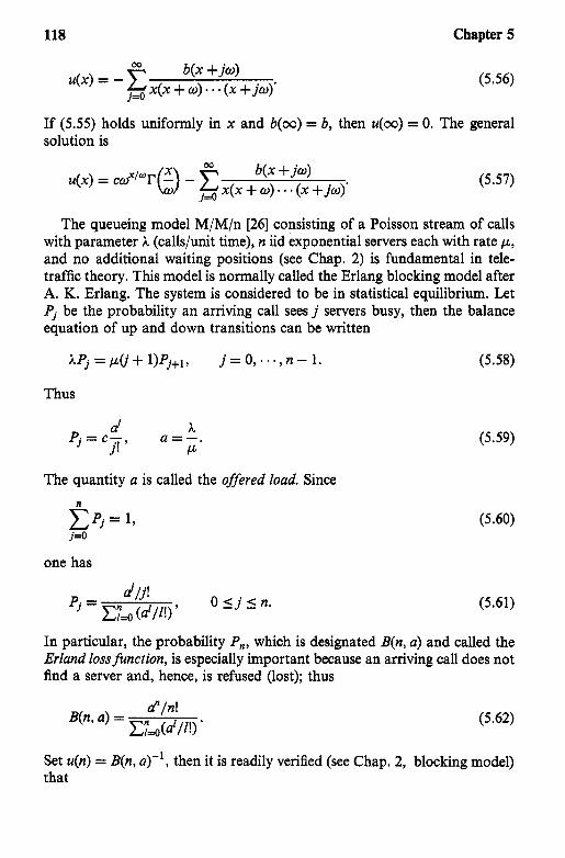
118 Chapter 5
b(x + j w ) = - x(x + W ) * ' (x +jw)'
(5.56) j=o
If (5 .55) holds uniformly in x and b(oo) = b, then u(oo) = 0. The general solution is
(5.57)
The queueing model M/M/n [26] consisting of a Poisson stream of calls with parameter A (calls/unit time), n iid exponential servers each with rate p, and no additional waiting positions (see Chap. 2) is fundamental in tele- traffic theory. This model is normally called the Erlang blocking model after A. K. Erlang. The system is considered to be in statistical equilibrium. Let Pj be the probability an arriving call sees j servers busy, then the balance equation of up and down transitions can be written
Thus
a' a. Pj = c T 1 a =--. J - P
The quantity a is called the offered load. Since
C P j = 1 , j=O
one has
(5.59)
(5.60)
(5.61)
In particular, the probability P,,, which is designated B(n, a) and called the Erland loss function, is especially important because an arriving call does not find a server and, hence, is refused (lost); thus
(5.62)
Set u(n) = B(nl a)", then it is readily verified (see Chap. 2, blocking model) that

The First-Order Difference Equation 119
u(n + 1 ) - - n+ 1 a
u(n) = 1 , u(0) = 1. (5.63)
The extension of the function B(n, a) to B(x, a) in which x is continuous is needed in many applications, including economic considerations in the sizing of trunk groups [27], approximations to the blocking model performance when the arriving stream of calls is not Poisson [28], and the construction of approximations of other important functions in teletraffic and queueing theory. The extension should be an analytic function of minimal growth and be uniquely determined by the condition B(0, a) = 1. Those conditions are met by the principal solution of the system
x + 1 .(X + 1 ) - -
a u(x) = 1 , u(0) = 1 ,
B(x, a) = u(x)-' . To solve (5.64), one may use
u(x) = a Y ( x + 1);
thus,
X a"+' U ( X ) = c a T ( x + l ) + a T ( x + 1 ) S- r(z + 2) "*
The solution provided by (5.38) is
thus,
(5.64)
(5.65)
(5.66)
(5.67)
(5.68)
This expansion is excellent for computation when a is not much greater than A..
The form of solution given by (5.40), namely
when directly interpreted by the definition of sum (Chap. 3), leads back to (5.68); also, using the identity (3.33), one again obtains (5.62) when x is an integer. Let x be an integer; then, by (5.62),

120 Chapter 5
(5.70)
= 2 ( X ) l ! d , I=O
hence
A'B(O, ~ 1 - l = W / . (5.71)
The Newton expansion, for x not necessarily integral, is, accordingly,
B(x, a)-' = c (x)l!a-' W
l=O (5.72)
This expansion is not convergent for any x not a positive integer; never- theless, because of its asymptotic character [29], it provides an excellent means of computation for a greater than x. For this purpose the expansion is continued until [x + a] (b] = integral part of y).
An integral representation for B(x, a)-' may be obtained from (5.72). Substituting
(5.73)
yields the Fortet integral formula
B(x, a)-' = a l e-a'( 1 + t)" dt m
(5.74)
from which other properties may be derived [29]. A technique that is useful in the study of the M/G/l queueing system
consists of equating the rate of up and down crossings of the level of work in the system. Denote the level of work in the system, considered to be in equilibrium, by y , and let the corresponding density function be f ( y ) . Consider the ( t , y ) plane and the strip (y, y + dy), dy > 0; then the probabil- ity the level of work in the system is in the strip is f(y) dy.
Now consider a down crossing of the sample path of work in the system through the strip due to depletion of the work by the server; the time required to traverse the strip is dt. Let N be the mean number of down-

The First-Order Difference Equation 121
crossings per unit time; then, because the arrival stream is Poisson, the probability the work level is in (y, y + dy) is also given by N dt; hence
fb) dy = N dt. (5.75)
Define the server rate gb) by
(5.76)
(5.77)
The next example to be considered is an M/G/l queue with exponential reneging. Let the complementary distribution of service time be B@) and the complementary distribution of reneging be e-Wy; thus, when a customer joins the queue, he may leave at any time before starting service with prob- ability W dt. Once service is started, he will not leave until service completion. The arrival rate is h, the service rate is p, and the server rate is one. From (5.77), the following integral equation of Volterra type is obtained:
fb) = hPBW + h / h B b - e F 4 4 (5.78) 0
in which P is the probability the system is empty. The terms of (5.78) arise as follows. The left-hand side is the rate of
down-crossing. The term hPB(y) means a customer arrives to find an empty queue and brings work in excess of y , thus causing an up-crossing of level y ; alternatively, the arriving customer could find an amount of work already in the system in the interval @ , e + de) for which the probability is f(6) de, brings work in excess of y - 6, and will not renege until past the time 6. The integral provides the total contribution of these customers, each one of which causes an up-crossing; thus, the right hand side is the total up- crossing rate. Since the queue is in equilibrium, (5.78) is obtained. It may also be observed that, since h is the arrival rate, the quantity fb)/A or, equivalently,
PS@> + /yf(e)Bb - de (5.79) 0
is the probability an arriving customer causes an up-crossing of work level y. Using Laplace transforms, (5.78) becomes
f ( s + W ) - h-l&s)-lf(s) = -P, f(0) = 0. (5.80)
To satisfy the boundary condition, the form of solution (5.34) will be used; accordingly, one has

122 Chapter 5
(5.81)
Clearly, conditions (5.39, (5.36) are met with aj = 0 (j 2 0). From
f(0) = S W f b ) d y = 1 - P (5.82) 0
one has
(5.83) j=O k=O
This provides a practical way to obtain the emptiness probability P;, how- ever (5.81) is usually difficult to use for the explicit inversion of f ( s ) to obtainfb). The M/M/l case may, however, be carried through. Let
(5.84)
then
From 1 1
S($ + 1) * * . (S + j ) j ! c -(I -e-Yy', (5.86)
one has
(5.88)
The z, p operators to be studied in Chap. 7 can provide a solution in inverse factorial series; this can supply a practical means of invertingf(8).
4. THE DIFFERENTIAL-DIFFERENCE EQUATION
The form of equation to be considered is

The First-Order Difference Equation 123
(5.89)
Such equations were studied by Truesdell [3], who developed a technique of solution based on the equation
a -F(& x) = F(z, x + 1) az (5.90)
which he called the “F-equation”. Let zo be a fixed value for which F(z0, x + r) = +(x + r) (5.91)
is known for all integral Y z 0; then the unique solution of the F-equation satisfying the boundary condition (5.91) is given by
00
F(z, X ) = x- (’ - +(x + r) . r! r=O
Equation (5.92) follows on observing that
(5.92)
(5.93)
and then using Taylor’s series. A theorem guaranteeing this result is the following (Truesdell): let I+(a)I 5 M for some M and all R(a) 2 ao; then a unique solution, F(z, a), of the F-equation exists such that F(z0, a) = +(a) for R(a) z ao, is an integral function of z for each a, and is represented by the Taylor series of (5.92). Thus a solution of the original differential- difference equation (5.89) would be available if it could be transformed to the F-equation.
The first step in the reduction procedure is the substitution
v(w, x) = ,-.lw: dy u(w, x). (5.94)
This leads to the equation a -v(w, x ) = c(w, x)w(w, x + l), aw
c(w, x ) = B(w, x)e 1; A A ~ J ) dy 7
(5.95)
in which A operates with respect to x . Further reduction of the equation cannot be accomplished unless c(w, x) has the form
C(W, X ) = D(w)E(x). (5.96) This will now be assumed so that
a -w(w, x) = D(w)E(x)v(w, x + 1). (5.97) aw
, .. , , ., . _ _.._ ..., . ,..._ . ,_ ,.., ~ ..,.,. .,....,..._. . .. . . I . .. .I . , I . . . .. ... . .. . . . . . . , . , . .

124
Let
z = 6 D W d X w(w, x) = h(z, x),
then a
-h(z, x) = E(x)h(z, x + 1). aZ
The final change of variable is X
F(z, x) = ex h(z, x), S 0 In E(z)Az
then a -F(z, x) = F(z, x + 1). az
e',
Examples of solutions of the F-equation (5.90) are [3]
sin(z -;x),
eixn r(x)z-x, eixnI'(x + l)F(b, c; -x; a), hypergeometric,
eixn-z~f)(z), Laguerre, &xn-z z -1 B(x, z)-', Erlang B,
eiXzz-X'2Jx(2,/3, Bessel..
An example of (5.89) is
Chapter 5
(5.98)
(5.99)
(5.100)
(5.101)
(5.102)
a aw --(W, X) = -(A + ,UX)U(W, X) + /A(X + ~)u(w, X + l), zo = 0. (5.103)
The condition imposed is that u(0, x) is specified. Using (5.94) with wo = 0, one gets
v(w, x) = e(*tpx)wu(W, x), a
aw -w(w, x) = p(x + l)e-pww(w, x + l), in which the condition (5.96) is met. From (5.98), one has
1 - e-pW P
Z = 9
The choice w1 = 0 is made, ensuring W = 0 z = 0. Thus
(5.104)
(5.105)

The First-Order Difference Equation
a -h(z, x ) = /.&(x + l)h(z, x + 1). az
Use of (5.100) leads to
F(Z, X ) = P x r ( x + I ) ~ ( z , X ) ,
a ”F(z, x) = F(z, x + 1). az
125
(5.106)
(5.107)
Stepping back from (5.92) through the changes of variables yields the solution
(5.108)
in terms of the initial data u(0, x + r) . The expansion provides the unique solution of (5.103) if lu(0, a)I 5 M for R(a) L ao, R(x) L ao.
The following example concerns the GI/M/I queueing model. The arriv- ing stream of customers is assumed to constitute a renewal process with interarrival time distribution F(y) and mean arrival rate h. The service dis- tribution is 1 - e-@’. Define g(t) by
in which
f = m , F C ( t ) = 1 - F(t ) .
(5.109)
(5.1 10)
The expression g ( t ) d t is the probability of an arrival in (t, t + d t ) given that the last arrival point is t units of time back. The function g(t) is called the “rate function” of the arrival stream. The queue is assumed to be in equilibrium and the state is (n, t) at the observation time t. Thus, at time t , there are n customers in the system and the last arrival occurred t units of time ago. It is required to determine the corresponding density function 4n(t)*
Since
4 n ( d + (P + g(t))qfl(t) (5.111) is the rate of leaving the state (n, t) and
P4n+l ( t ) (5.1 12)
is the rate of entering, one has the state equation

126 Chapter 5
For n = 0, one has the boundary condition
do(@ = -g(z)qo(t> + Pql(t)*
Using (5.94)
(5.1 14)
and setting
(5.1 17)
Thus, use of the Taylor series and substitution back to qn(t) provide the solution
(5.118)
Since it is known [30] that the probability, IC,, that an arriving customer sees n in the system is
7t" = (1 -@)W", n I 0, (5.119)
&(l - W ) ) = W , 0 < W < 1, (5.120)
in which W satisfies the equation
it seems reasonable to assume the form Aw"(n 2 1) for q,(O) for some A , W .
Thus, from (5.1 18), one has
qn(t) = Awne-P("u)rFC(t) . (5.121)
The boundary condition
(5.122)
and (5.121) yield (5.120) thus identifying this W with that in (5,119). Let P, be the probability that there are n in the system at the observation time t; then
(5.123) F P n = 1. n=O

The First-Order Difference Equation 127
To determine PO, the following conservation argument may be used: in equilibrium, the mean rate of arrivals into the queueing system must equal the mean rate of departures; thus
A P
Po = 1 --.
A. P
P, =-(l - W)W"", n 2 1,
(5.124)
(5.125)
(5.126)
For the function qO(r), the boundary condition (5.1 14) gives
q o ( d = [40(0) + A. - he lFC(t). (5.127) -p( l -o)r
To obtain qo(O), one may use W P o = l qo(r) dt = qo(0)A." + A.
- - W ) ) = qo(o)A.-' + A. - - A. P(1 - 4 P '
(5.128) Thus qo(0) = 0 and
qO(r) = - e-~" ("~ ) ' ]~~ ( ( t ) . (5.129)
A further example of the Truesdell reduction is given by an application to the coefficients A,@) (3.231). A representation will now be obtained that will permit computation when W is small and will also prove (3.238).
Setting
so that
one has (3.204)
(5.130)
(5.131)
128
d
Use of the identity
provides the equation
d d o -a,(o) = -va,(w) - (v + l)a,+1(4,
which has the required form (5.89). Let
a,(w) = e"'ww,(w),
then
d - v,(w) = - (v + l)e-ww,+~(o). d o The substitutions
z = 1 - e-w,
%(4 = h"(4
yield
d dz "h,(z) = - (v + l)h,+l(Z).
Using the notation
(a)o = 1, (a), = a(a + 1) (a + r - l), r 2 1,
one has
and, hence, the Taylor expansion of h,(z) about z = 0 is
Chapter 5
(5.132)
(5.133)
(5.134)
(5.135)
(5.136)
(5.137)
(5.138)
(5.139)
(5.140)
(5.141)
Stepping back through the substitutions (5.137), (5.135) and using the boundary values (5.132), the following expansion is obtained:

The First-Order Difference Equation 129
(5.142)
The final expansion is now obtained after use of (3.214) and (5.130), that is,
(5.143)
5. DERIVATIVE
The derivative, u’(x), with respect to x of the solution, u(x), of (5.27) will be considered. This often provides important information concerning physical models described by the difference equation. Of course, if one has a suffi- ciently tractable explicit solution, then the derivative may be obtained imme- diately. One may also use the following difference formulation for u’(x) obtained from (5.27):
u’(x + W) - a(x)u’(x) = d(x)u(x) + b’(x). (5.144)
This presupposes that #(x) has been obtained and that a suitable boundary condition on u’(x) is available. Thus from
(5.145)
(5.146)
For the Erlang loss function, the derivative, M ( x , a)/ax, is especially important in the economic sizing of trunk groups in teletraffic studies [27,31] and in real-time computations for the routing of teletraffic through networks [32]. Thus, from (5.64), (5.74) one has
u’(x + 1) - 7 + u’(x) = -u(x), 1 a
In this case, however, one may also write
(5.147)
(5.148)

130 Chapter 5
For the M/G/l model of (5.78), the quantity -f'(O) is the mean work in the queueing system and, hence, the mean waiting time of a customer in first out, first in discipline. This may be obtained from (5.80) by differentiation; thus,
It may be observed that the formulae of (5.147), (5.148), while useful for the study of aB(x, a)/ax, are not suitable for convenient real-time computa- tion. Similarly, (5.149) is awkward for computation. Thus, because of the importance of the general problem, it would be useful to obtain an approx- imation for u'(x) of (5.27) that would be suitable for rapid computation. Accordingly, rewriting (5.27) in the form
u(x + W)u(x)-l = a(x) + b(x)u(x)-l, (5.150)
one has 1
A 1ri u(x) = -In(a(x) + b(x)u(x)") (5.151) W W
and, hence, 1 2 In u(x) = c + - S In(a(z) + b(z)u(z)") A Z. W X0 W
Differentiation yields
(5.152)
(5.153)
Finally, using the Norlund expansion (3.171) for v = 1 and solving for u'(x)/u(x), one gets
u'(x) W-l (a(x) + b(x)u(x)) - 4 (a'(x) + b'(x)u(x)"') u(x) - a(x) + ib(x)u(x)" " (5.154)
This provides a reasonably accurate approximation to u'(x)/u(x) on the supposition that u(x) has already been obtained.
Application of (5.154) to (5.145) yields the familiar

The First-Order Difference Equation
Table 1 Approximation of -B"aB/ax.
131
X a -B"aB/ax Approx.
5 1.3608 1.4025 1.4044 10 4.4612 0.8626 0.8630 20 12.0306 0.5406 0.5406 50 37.9014 0.2956 0.2956
1 2x
+(x) 2 lnx - -. (5.155)
An important application is to (5.64) from which one gets
a=- x + ' + B(x, a). U
(5.156)
Table 1 illustrates the accuracy of (5.156). Throughout the table,
An application of (5.154) will now be made to the M/G/l model of (5.80) in order to approximate -y(O) and hence the mean waiting time. One has
B(x, a) = .Ole
a(s) = A-'/qs)-', b(s) = -P.
(5.157)
The quantity &O) = p-' is the mean service time and p is the service rate; also, p = A / p is the offered load in Erlangs. Hence
a(0) = p-' ,
a(0) + b(Of(0) = p-1 - - P 1 -P'
(5.158)
The quantity a'(0) = -A-' &O)-2p(0) is equal to $p-'pp2 in which p2 is the second moment of the service distribution. The recurrence time, R (mean unexpended service time of the one in service), is equal to $pp2 [33], hence
~'(0) = p-'R. (5.159) Let W be the mean waiting time; then the approximation obtained is
.! -IR - W-' (p-' w=(l-P) 2 p - P/(I - P)) In(p" - P/(I - P)) p-' - 4 P/(1 - P)
(5.160)
132 Chapter 5
It is clear from (5.151), that (5.160) produces the exact result, W = pR/(1 - p), for W + 0 + .
The following numerical example will provide a rough idea of the per- formance of the approximation. Let
= fe-2Y + ge-3~ , A.=2, @ = l , (5.161)
then
(5.162)
The value of P is found from (5.83) with - 1 1 1 1
B(S) = -- + --; 2 2 + s 2 3 + s (5.163)
it is P = .3771. Numerical solution of the integral equation (5.78) for this problem and subsequent numerical evaluation of y f b ) dy gave the result W = .401, while the preceding approximation gives W = ,395. These values can be considered to be in acceptable agreement.
It is clear that the second derivative, u"(x), may be approximated by starting from the difference equation for U'($, (5.144), and applying (5.154).
6. FUNCTIONAL EQUATIONS
A number of important stochastic models are represented by functional equations of the form
G ( W ) - W x z ) = m(z). (5.164) Usually +(z), l(z), m(z) are specified and G(z) is to be determined. As an illustration, consider an M/M/1 queue with arrival rate A. and service rate ,ul associated with these customers termed ordinary, and let there be a single customer whose rate is p2 and who always cycles back after service comple- tion to the end of the queue. The discipline is first in, first out. It is required to find the generating function, G(z), of the number of ordinary customers in the system assumed to be in equilibrium.
To formulate the equation for G(z), let J( t ) be the sojourn time distribu- tion (time spent by a customer in the system from arrival until departure); then the number of arrivals during the sojourn time is also the required number in the system. Let P, be the probability of n arrivals, then
and
(5.165)

The First-Order Difference Equation 133
W
G(z) = C Pnz" n=O
(5.166)
Substitution for P, into (5.166) yields
G(z) = .?(A - Az) (5.167)
in which
is the Laplace-Stieltjes transform of J( t ) . One may obtain .?(S) directly on observing that the Laplace-Stieltjes
transform of service time for the ordinary customers is p1/(s + pl) and that for the cycling (feedback) customer is P ~ / ( s + ~ 2 ) ; hence, if there are n arrivals, then the transform of the sojourn time distribution is (pz/@ + PZ))(Pl/(S + P1)ln; accordinglY,
.?(S) = - P2 G ( L ) . S+P2 $+P1
(5.169)
The functional equation for G(z) may now be obtained from (5.167) and (5.169), namely
G(z) = G ( ), W ) = 1, 1 + rp(1 - z) 1 + p(1 - z ) A P1
P1 P2
1
(5.170) p = - , r=-.
This equation will be resolved later; also, another view of its derivation and a generalization will be discussed in connection with branching processes.
The nonlinear difference equation
Z(t + 1) = +(Z(t)) , Z(0) = z (5.171) is fundamental in the study of (5.164). For our purposes, the more general form
+ z(t) = e(z(t)), z(o) = z, h > o (5.172)
is of greater utility. The full notation Z(t; zlh) will be used when dependence on all arguments is emphasized; otherwise just Z(t; z), Z(t) , or even Z as the occasion permits. The variable t is always considered to be continuous. It will be assumed that a unique solution, Z(t; zlh), of (5.172) exists possessing a derivative, Z , with respect to 1. An important function is
Z(0; zlh) = g(zlh), (5.173)

134 Chapter 5
which, in view of the time homogeneity of (5.172) and the uniqueness of the solution, provides the following differential equation:
i ( t ) = g(Z(t)) , Z(0) = z;
which is, therefore, equivalent to (5.172). From (5.174), one immediately obtains
and, in particular,
from which Z(t), O(z) may be calculated. An example is given by
(5.174)
(5.175)
(5.176)
then
Z Z 2 Z(t ) = - 1 - tz'
e(zlh) = - 1 - hz' (5.178)
Usually, however, O(z) is initially specified and is often independent of h; thus the determination of Z(t ) from (5.175) rests on obtaining g(z1h).
One may obtain a partial differential equation that implies (5.172) as follows:
Z(t ; Z ) = Z(t - dt, Z(dt)) = Z(t - dt; z + g(z)dt), (5.179) hence
(5.180)
This equation reduces to (5.173) at t = 0 and, hence, also implies (5.174).
[34]. The following example is from Mickens: Depending on the specific nature of &), (5.171) may be solved explicitly
Z(t + 1) = 2Z(1 - Z), Z(0) = z . (5.181) The substitution
z =;(l - V ) , V(0) = 1 - 22 (5.182)
V(t + 1) = V(t)2, (5.183)
yields
In V(t + 1) - 21n V( t ) = 0; (5.184)

The First-Order Difference Quation
hence
V(t) = (1 - 22)2',
Z(t) = i[l - (1 - 22)2'], z < 4. From (5.173), one obtains
In 2 2
g(z) = " (1 - 2z)ln(l - 2z), z 3. Of importance is the following example:
Z(t + 1) = a + bZ(t) c + dZ(t) ' Z(0) = Z, ad - bc # 0
with constant a, b, c, d . One has
Z(t + l)(c + d Z ( t ) ) = a + bZ(t) which is of Riccati form; see. Chap. 2 (2.14). The substitution
leads to ~ ( t + 2) - (b + c ) w ( ~ + 1) - (ad - b c ) ~ ( t ) = 0.
135
(5.185)
(5.186)
(5.187)
(5.188)
(5.189)
(5.190)
(5.191) The theory of linear difference equations with constant coefficients will be covered in Chap. 6; however, for the present the model of Chap. 2 (2.21)- (2.34) may be followed. Define a, B to be the roots of
X' - (b + C)X - (ad - bc) = 0; then, for a # B,
v(t) = A d + BB'.
One may now write Z(t ) in the form
1 a'+1 + K/?'+' c Z(t) = -
d a'+K/3' d ' "
and, hence,
Z(t) = - 1 (c + dz - B)a'+' - (c + dz - a)$+' c d (C + dz - B).' - ( C + dz - a)B' d '
"
For a = B, it may be verified that
w(t) = ( A + &)a';
(5.192)
(5.193)
(5.194)
a! # B. (5.195)
(5.196)

136 Chapter 5
thus,
Z(t ) = - a l + K + K t c d 1 + K t d '
"
and one now has
Z( t ) = - Q Q + (C + dz - a)(t + 1) C Q = p.
d ~ + ( c + d z - a ) t d ' "
For the corresponding infinitesimal generators, one gets
d g(z) = " ( z - Q = p. a
(5.197)
(5.198)
(5.199)
(5.200)
The difference equation (5.171) is important in the theory of branching processes [13,14,35] a sketch of which will now be given. A branching pro- cess may be considered to be a description of a birth-death population model. Let a single individual exist at time zero and let a probability dis- tribution pj (j L 0) be defined with the interpretation that p0 is the prob- ability the individual dies after one unit of time, p1 is the probability the individual survives but has no progeny, and pi (j 2 2) is the probability the population consists o f j individuals. After another unit of time, each indi- vidual acts independently with the same associated probability distribution. Let x. = 1 and let x, designate the population at the end of r units of time also let p:) = p [ x , =l1 (thus pj') = Q), then the following generating func- tions may be defined:
4 0 M = z, m
d(z) = C p j z j , $(l) = 1. j=O
(5.201)
The function Z(r; z)defined by
Z(r + 1; z) = +(Z(r; z), Z(0; z) = z (5.202)
and considered as a function of z is the generating function of p:) ( r L 0). This constitutes a discrete branching process.
Of interest in these processes is Z(m; z) , p i@. Since $(z) is monotone increasing, Z(r; z) is also monotone increasing in r; further, since Z(r; z) is bounded, one must have Z(m; z) = c, in which c is the smallest root of 4(z) = z. Let m be the mean of the one-step population distribution, that is, m = 4'(1); then, by the convexity of #(z) for z E [0, l], m > 1 implies c <
The First-Order Difference Equation 137
1, and m I 1 implies < = 1. Thus, unless m > 1, extinction is certain. One may obtain this condition analytically by setting
f ( z > = 9(z) - z; (5.203)
thenf(1) = O,f'(l) = m - l,f"(z) 2 0 (z E [0, l ] ) , hence
@(z) 2 z + (z - l)(m - 1) (5.204)
and
(5 - l)(m - 1) 5 0. (5.205)
It follows that m > 1 j < < 1, and m f 1 j <= 1. The function g(z) = Z(0; z ) may be interpreted in terms of multiplicative
processes in continuous time. Let x(t ) be the population size at the time t with x(0) = 1, then
Z(t; z ) = EZx('). (5.206)
Since
Z(dt) = z + dZ = z + g(z) dt, x(dt) = 1 + dx,
(5.207)
one has
z + g(z)dt = E[z1+q. (5.208)
Let infinitesimal transition rates, p , ak, be defined by
P[& = k] = ak dt, k ? 1, P[dx = -l] = p dt,
(5.209)
then W
P[dx = 01 = 1 - p + C a k dt [ k=l } and
thus,
(5.210)
(5.211)
(5.212)

138 Chapter 5
One may observe that g( 1) = 0. The corresponding population size generat- ing function, Z(t; z), and the one-step (step size h) finite form, +(z), may be obtained from (5.175) and (5.176), respectively (+(z) = z + hO(z)).
The simple birth-death model in which p is the death rate and h is the birth rate is, accordingly, given by
g(z) = p - (p + h)z + hz2. , (5.213)
The corresponding Z(t) is obtained from
dv L= (v - l)(hv - p) = t. (5.214)
One has
z - 1 "- z - 1 e(&& z - p/). - z - p / h
(5.215)
and, hence,
(5.216)
The case h = p may be obtained as the limiting form of (5.216); it is
Z(t) = 1 + z - 1 1 - (z - 1)At' h = p, (5.217)
The one-step forms are
z - 1 h = p. = l + l - ( z - l ) X h '
Thus Z(t) satisfies
Z(t + h) = +(Z(t)), Z(0) = 2
(5.218)
(5.219)
(5.220)
for continuous t p 0. The question of the solution of functional equations of the form (5.164)
will be reconsidered after the development of methods for the solution of difference equations (5.172).

The First-Order Difference Equation 139
7. U-OPERATOR SOLUTION OF AZ = e(z> h
Methods will now be discussed for the solution of (5.172). Newton’s inter- polation, Chap. 1 ( lag) , will form the basis for the first approach. From (5.172), one has
Z(t + h) = Z(t ) + W , W = he(Z(t)). (5.221)
The operator U is now introduced and defined by
in whichf(z) is any given function (the domain of U and thus restrictions of the operator will depend on the applications). Thus
US@) = p t ) l f = o
1 h
(5.223) = - Lf(z + he(z)) -f(z)].
Similarly, one has
W Z ) = *jf(Z(t))It=o. (5.224)
Thus Newton’s formula provides the following solution:
and, in particular,
Z(t) = c (,t’h)PUjZ, 00
j=o
(5.225)
(5.226)
The expansions (5.225) and (5.226) are formal; i.e., convergence is not implied. Normally the expansion is used in the form
(5.227)
R, = ( i h ) h m Umf (z).
Thus the error is estimated by the next term. The operator U is a direct analogue of the Lie-Grobner operator [4] used
in the study of simultaneous differential equations. In fact, for h -+ 0+, one expects

140 Chapter 5
(5.228)
if the limits exist. One may write (5.225), (5.226) in the symbolic forms
(5.229)
(5.230)
One may establish a relationship of (5.229) to semigroups [36]. Define the norm off(z) by
and the family of operators T(t) by
T(t)Z(O; z ) = Z(t; z) , T(0) = I (identity map);
then
T(t) = (1 + hU)?
The infinitesimal generator, A , of the semigroup is defined by
Af(z ) = lim - [T(kY(z ) - I f (z)]; 1 k+O+ k
hence 1 h
A = -ln(l + hU)
and
A m = g(zY"(z), AZ = g@).
Hille's representation of the semigroup is
(5.231)
(5.232)
(5.233)
(5.234)
(5.235)
(5.236)
The First-Order Difference Equation 141
(5.237)
which, for functions Z ( t ; z ) analytic in a circle about the origin, may be written
(5.238) Ar = e z.
The differential equation (5.174) is now an immediate consequence of (5.238). The differential equation (5.180) follows directly from the semi- group property
T(t + t) = T ( t ) T ( t ) , (5.239) which is taken to be the defining relation for semigroups. The approach through semigroup theory will not, however, be pursued further here.
The partial sum of (5.227) is, of course, exact when t has one of the values 0, h, . . . (m - 1)h and may be expected to be accurate for t E [0, (m - l)h]; however the accuracy also depends on h and the choice off(z). An example of the latter dependence is given by the function F(z) defined by
UF(z) = 1 (5.240)
for which (5.225) yields immediately
F(Z(t)) = F(z) + t , (5.241)
which is exact for all t . The function F(z) is an invariant of the operator U ; it is simply related to the infinitesimal generator. Differentiation of (5.241) with respect to t at t = 0 provides the relation
F’(z)g(z) = 1. (5.242)
Guided by this relation, (5.228) shows that the function f ( z ) defined by f’(z)O(z) = 1 in (5.227) may be expected to provide good accuracy.
Consider the example 1
A z(t) = - h Z ( t )
Z(0) = z.
Usingf(z) = z, m = 3 in (5.227), one has
Uz=-, I
Z
2 1 U z = - z(z2 + h) ’
(5.243)
(5.244)

142 Chapter 5
and hence
Z(t; zlh) 2: z + - - t t(t - h) z 2z(z2 + h)
Alternatively, choosing f(z) = z2/2, which satisfies f '0 = 1, one has
Z2 h U - = l + - 2 222 ' z2 2hz2 + h2 U -= - 2 2zyz2 + h)2
and hence
Z(t; zlh)2 2: z2 + t t(t - h) 2hz2 + h'
(5.245)
(5.246)
(5.247)
Noting that Uz2/2 differs from 1 by h/(2z2), accuracy may be expected to be good when h/2z2 is small. Evaluation of Z(.7,51.5) by (5.227) using m = 9 yields the value 5.139444480 correct to the last figure. Use of (5.245) yields 5.139450980 with the error -6.5e - 6, and (5.247) yields 5.139444332 with the error 1.48e - 7, providing a reduction of error of 44 times.
For another example consider
A z( t ) = --z(#, Z(0) = z. (5.248) h
For f(z) = z, one has
and for the choice f(z) = l/z, one gets
"-+"- 1 1 t t(t - h) hz2 Z(t; zlh) - z t - hz 2 ( l - hz)(l - hz + h2z2) m
(5.249)
(5.250)
Since Ul/z = 1 + hz/(l - hz), one may expect good accuracy if hz is less than 1 and small. Using (5.227) with m = 9 yields Z(.3; S1.2) = .4287462 correct to the last figure. From (5.249), one computes ,4287211 with the error 2.5e - 5, while from (5.250) one gets .4287455 with the error 6.5e - 7; thus a reduction of error of 38 times is achieved.
The value of t , as previouly noted, should be chosen within the range of nodal points used in order to maintain the interpolatory character of the Newton expansion. For the first example, they are 0, .5, 1 and for the second example 0, .2, .4. The computation of Z(t) for values of t outside the nodal point range may be done in stages by successively using the values Z(t) obtained as initial values for succeeding computations.

The First-Order Difference Equation 143
An expansion for g(z) may be obtained from (5.235) and (5.236), thus 1
g(zY”(z) = iln(1 + hUY(z) , (5.251)
Thus one may again obtain (5.242) from (5.240). One may, accordingly, expect the same sort of improvement in the computation of g(z) from (5.251) by the use off(z) defined in (5.244). For this choice, one has
Applying (5.252) to the problem of (5.243), one gets
1 h h2 2z2 + h g(z) 2: ; + - + - 2z3 4 z3(z2 + *
For the problem of (5.248), one gets
z2 1 h2z4 g(z )2: --”
1 - hz 2 (1 - hz)( 1 - hz + h2z2)
(5.252)
(5.253)
(5.254)
8. CRITICAL POINTS
From here on, e(z ) of (5.172) is assumed to be independent of h. The zeros, a, of O(z) are termed the critical points of the difference equation or points of equilibrium. Clearly, Z(t ) is identically equal to a for any choice of h if z = a; thus Z(t) is also identically zero, hence g(z) also vanishes at a. A critical point is termed repulsive if, for z in a half-deleted neighborhood of a,Z(t) moves away from a as t increases; conversely, if Z(t ) moves toward a, that is limr+oo Z ( t ) = a, then a is termed attractive. To obtain a criterion for deciding the character of a, let
Z( t ) = a + &(t); (5.255)
(5.256)

144 Chapter 5
Let r be the first index for which &)(a) # 0; then, using the Taylor expan- sion of e(z) about a and ignoring terms beyond ~ ( t ) ‘ , one has
e(‘)(a) A ~ ( t ) = -~(t)‘, h > 0, E ( 0 ) = E o . h r!
(5.257)
For r = 1, one has
E f t + h) = (1 + hBI(tx))E(t), (5.258)
hence, a is attractive if
11 + he’@) I < 1 (5.259)
and repulsive if
1 1 +he’(a)I > 1. (5.260)
A simple criterion for r > 1 and h sufficiently small may be obtained by replacing (5.257) by
i(1) = - E ( t ) ‘ , r! E ( 0 ) = E o .
Thus
(5.261)
(5.262)
consequently, a is attractive if d’)(a) < 0 and repulsive if &)(a) > 0 when EO > 0. If 0 then the same conclusion is reached for r odd; however, the conditions are reversed for r even. These conditions for r > 1 are summar- ized in Table 2.
Consider the following examples:
Table 2 Classification of Critical Points for r > 1
Attractive Repulsive

The First-Order Difference Equation 145
hence, for 0 h < 2, a! is attractive. 2. e(z) = c(z - - c), c 0.
a! = 1, 3, e‘(1) = c(1 - C), e‘(<) = c(< - 1).
Thus: 0 < c < 1 =+ a! = 1 is repulsive, and for 0 h 2/41 - c), a = < is attractive; < > 1 j Q = 1 is attractive for 0 < h 2/c(< - l), and a = f is repulsive; < = 1 yields a double root for which O”(1) = 2c, hence, so
0 =+ a! = 1 is attractive, > 0 =$ a! = 1 is repulsive for sufficiently small h.
3. e(z) = Z(I - 22).
a = o,i,e’(o) = 1, e‘(;) = -1.
Thus a! = 0 is repulsive, and a! = $ is attractive for 0 h 2. 4. e(z) = Z ~ ( Z - 1).
= 0, 1, e”(o) = -2, e‘(1) = 1.
Hence a! = 1 is repulsive, and, for h small enough, a! = 0 is attractive when 0, otherwise repulsive for 0.
9. A BRANCHING PROCESS APPROXIMATION
A function, @(z), is said to be absolutely monotone on z E [0, l] if
&)(z) 2 0, r = 0,1,2, . . . (5.263)
It is known @(z) is necessarily analytic, and if further @( 1) = 1, then it is a probability generating function. For this class of functions, an approxima- tion will be obtained for the system
Z( t + 1) = @(Z(t)) , Z(0) = 2. (5.264)
Three cases are distinguished according to @’( 1) > 1, @’( 1) 1, and @’( 1) = 1. The infinitesimal generator of the approximations will always have the form
g(z) = c(z - l)(z - C). (5.265)
Case 1: @’(l) > 1 (supercritical case).
It is clear that there is just one number f E (0, 1) satisfying @(C) = 5. This is taken for c in g(z). Using (5.175) or, equivalently, (5.216), one obtains the following approximation, 2(t; z ) to ~ ( t ; z):
(5.266)

146 Chapter 5
The mean number in the population, m(t), is given by
(5.267)
Let m = m(1); then, since #(z) is the exact one-step generating function, one may take m = q5'(1), hence the final approximation is
m = #'(l), -
Z(t ; z ) = z - 5 - ( z - 1)gm' z - ( - (z - l)m' '
m(t) = m!, (5.268)
g(z) = -(z - l)(z - 5). In m I - <
Case 2: J(1) < 1 (subcritical case).
It will be assumed that #(z) may be analytically continued so that a value 5 > 1 exists satisfying +(c) = 5. The smallest such root is chosen and used in g(z). Again, setting m = r$(l), one finds exactly the same solution, which is given in (5.268).
Case 3: #'(l) = 1 (critical case).
One may take
g(z) = c(z - yielding
2(t; 2 ) = 1 + z - 1 1 - (z - 1)ct '
(5.269)
(5.270)
(5.272)
Let the probability distribution generated by +(z) be p0 ,p1 , . . ., then (5.272) ensures that 2(t; z ) generates the same value of p o .
It is clear, from the construction of the approximations, that 2(t; z ) is exact when #(z) is a bilinear form.
Example: Let B(x) be the distribution function of a nonnegative random variable with Laplace-Stieltjes transform &S), i.e.,

The Hrst-Order Difference Equation 147
(5.273)
then, since &S) is completely monotone, it follows tha: @(z) = &h - hz) (A =- 0) is absolutely monotone; further, since #(l) = B(0) = 1, #(z) is a probability generating function that may be used to define a branching process. If h is the arrival rate of a Poisson stream and B(x) the service time distribution of a queue, then m = #'(l) is the offered load p; the known stability condition, p < 1, implies the subcritical case, which further implies m(t) -+ 0, t + oo.The function Z(n; z ) (n = 1,2, , , .) is the probability gen- erating function of the number of arrivals after n consecutive services. For the choice B(x) = 1 - e-@', the approximation is exact, in this case, = l / p .
IO. A PERTURBATION SOLUTION OF A Z = e(z> h
It will be assumed that Z(t; zlh) is analytic in h about h = 0; further, O(z) is taken to be independent of h. Terms of the perturbation expansion in powers of h up to h' will be obtained. This can also provide significant information concerning the dependence of Z on t and z . Accordingly, let
Zo(t; z ) = Z(t; Z I O ) ,
so that
Z = Z o + h Z 1 + y Z z + . h2
with the initial conditions
z, = z , 2, = 0, Z2 = 0, etc.
(5.274)
(5.275)
(5.276)
the corresponding expansion for O ( Z ) is
e(z) =e(z,) + hz,e'(z,) h' (5.277) + y [Z,S'(Z,) + z:e"(z,)l+ ' ' *
The difference equation and initial condition may be written in the form
148 Chapter 5
(5.278)
(5.279)
+ h[ ZIe’(Z0) du - f e(Z0) + f I’ (5.280)
+ h2[iJi { Z ~ ~ ’ ( Z O ) + Z$”(Zo)} du - iz,e’(zo) + he(zo) -he(z)] + . . . .
Equating corresponding powers of h in the expansions of (5.275) and (5.280) and subsequent differentiation yields the following differential equations:
io = e(zo), i, = zlB‘(zo) - jzoe’(zo), iz = 4z2e‘(z0) + i z:e”(zo) (5.281)
- +ile’(zo) - $zlioe”(z0) +&zoe’(zo). Defining M(z) by
one may verify the following solutions of (5.281):
(5.282)
(5.283)
The First-Order Difference Equation 149
Thus the perturbation solution, (5.275), is now
(5.284)
+ & IB'(Z0) - d(Z) + M(Z0) - M ( z ) } ] + * * . Applying (5.284) as far as the first power of h to the examples of(5.243) and (5.248), one obtains respectively
Z(t ) = +
Z(t ) = - - 4 J m
h ln(l+$) +... Z
2
1 + t z h(&) ln(1 + tz) + ,
7
(5.285)
An additional example is provided by
A z = e-', Z(O) = z
for which one easily obtains h
Z( t ) = z + ln(1 + te-") +-e h In( 1 + te-") 2 1 + te-"
+ . * m .
(5.286)
(5.287)
11. HALDANE'S METHOD FOR AZ = O(Z)
The final method of solution to be discussed is due to J. B. S. Haldane [8]. It consists of determining the function F(z) of (5.240) or, equivalently, by (5.242), g(z)-' . One has
h
F(z) = [g(w)-' dw,
F(z + hO(z)) - F(z) = h.
Let
then, from (5.288),
(5.288)
(5.289)
(5.290)

150
For the integrals in (5.290), one may write
hence,
Chapter 5
(5.291)
(5.292)
Equating corresponding powers of h provides the following formulae:
1
I qZ)I-s+l c s!(l - S + 1). ,f,(l-qz) = 0, l 2 2.
S= 1
(5.293)
(5.294)
(5.295)
Examples are: 1
1. e(z) =-, Z

The First-Order Difference Equation 151
h h2 22 423
2 2 8z2
g(z)" = z ----+..., F(z)=Az2--lnz+-+.. h h'
. . 1 h h2E
g w ' = -2 + - + " z + . * * 1 h' E
F (z)=-+hlnz+-z+. - . EZ 2
3. e(z) = e", ha h2a2 2 6
F(z) = - -e 1 -a2 ha h2ae, +, , .
g(z)" = e-@' + - - - ea' + . . .
Q ,
+ T Z " 6 The determination of Z may be accomplished either by solution of the
system (5.174), namely
2 = g(z), Z(0) = z (5.296)
F ( Z ) = F(z) + t. (5.297) or by solution of the finite equation [see (5.175)]
12. SOLUTION OF G($(z)) - /(z)G(z) = m ( ~ ) .
Having discussed the nonlinear difference equations (5.171) and (5.172), it is possible now to return to the original equation (5.164). Define Z( t ) as in (5.171); then the functional equation may be written as
G(Z(t + 1)) - I(Z(t))G(Z(t)) = m(Z(t)) . (5.298) Let
U(t) = G(Z(t)), 4 t ) = I(Z(t>), b(t) = m(Z(t)).
Then (5.298) takes the form U(t + 1) - a(t)U(t) = b(t),
which was discussed earlier. Of course, one now obtains G(z) from
(5.299)
(5.300)
152 Chapter 5
G(z) = U(0). (5.301)
It is now possible to solve the functional equation (5.170) for the'M/M/I queue with a feedback customer. Defining Z ( t ) by
Z ( t + 1) = 1
1 + p( 1 - Z(t)) ' Z(0) = z
and using (5.195), one finds
Z ( t ) = 1 - pz - (1 - z)pf
1 - pz - (1 - ,)p'+' '
Setting
(5.302)
(5.303)
(5.304)
the functional equation becomes U(t + 1) - a(t)U(t) = 0, U ( m ) = 1. (5.305)
The boundary condition follows from Z(a0) = 1 , G ( l ) = 1. Thus, the required solution for U(t ) is
I Slna(w)Aw. U(t) = e m I
hence, O S a(w)Aw. G(z) = e m I
W
= n [l + up(1 - Z(j)) ] - l *
(5.306)
(5.307)
j=O
A perturbation solution for G(z) when Y is near one is readily obtained; let Y = 1 + E , then
a(t) = 1 + p(1 - Z( t ) ) + EP(1 - Z(t)) , (5.308)
and 0
G(z) = exp[S In( 1 + p(1 - Z(w))Aw] exp W
(5.309)

The First-Order Difference Equation 153
A simple general formulation for the solution of the equation
G(#(z)) - G(z) = 4 z ) (5.310) is obtained as follows. The substitutions (5.299j lead to
A V(t) = b(t) (5.31 1)
and, hence, to t
G(Z(t)) = K(z ) + $m(Z(w))Aw. (5.312)
Differentiation with respect to t at t = 0 yields 0
G’(z)g(z) = ~ ( z ) + H m’(Z(w)>Z(w)Aw (5.3 13)
which permits determination of G(z). Consider the example
One has
Z( t ) = - 1 + t z ’
g(2) = -22; Z
hence
1 0 1 G’(z) = -;+S
0 (1 + wz)2 Awn
The change of variable W = y / z gives
1 l 0 1 G’(z) = --+-S- A Y’
z Z O ( l + y ) 2 z
and the further change W = 1 + y gives
1 1 1 1 2 Z 1 W 2 I
G’(z) = - - + - S - - W .
From Chap. 3 (3.74), one has X1
$ ( X l Z ) = S; 4 W ,
hence
(5.314)
(5.315)
(5.316)
(5.317)
(5.318)
(5.319)
(5.320)
.. , . .. .. . . . . . . . . . _ .“ ........ .. .. . I . . ... .

154
Since, from (3.78),
one gets
and, finally,
G(z) = $(L). Z
Chapter 5
(5.321)
(5.322)
(5.323)
13. SIMULTANEOUS FIRST-ORDER EQUATIONS
Here, the theory of the first-order nonlinear difference equation is extended to a system of simultaneous equations. In what follows, it will be useful to use the notation 2 for the vector (21, 2 2 , a , x,) with scalar components 1 5 i 5 n. The general form of the system to be discussed is
A zj(t; 3 = e , ( i ) , ~ ~ ( 0 ; 3 = z j , 1 5 i 5 n, h (5.324)
Z’=(z1,zz,,**,z,),
in which ei(3 are independent of t . Define the infinitesimal generators g,(3 by
(5.325)
then, because of time homogeneity, the following system of differential equations is equivalent to (5.324):
dZi -= dt
gi&, z~(o) = zi, 1 5 i 5 n. (5.326)
The consideration
Z*(t + S ) ; 2) = zi(t; i ( S ; a), Iv zj(t; i+ ;;S>, S “P 0
shows that the partial differential equation
(5.327)
(5.328)

The First-Order Difference Equation 155
is also equivalent to (5.324); the solutions of (5.328) are the n functions
In order to construct the solution of the system (5.324), a U-operator approach will be followed. The total difference quotient with respect to t , A, implies h
Af(&)) h = i l f ( i ( t + h)) -f(%))l. (5.329)
Z,(t; 2).
Setting
wi = h8i(2), Zi(h) = z j + w j , (5.330)
one has
hence
W(z3 = +f(&))Ir=o. (5.333)
Clearly, one also has
in which Uo is taken to mean the identity operator.
ive of partial differentiation [8]. Define A by It is possible to put the definition of U into another form that is suggest-
Af(3 =f(; + 2) - f (2) , in which the wi are treated as constants; then
A =E? ...E," - 1;
(5.335)
(5.336)
the Ej are translation operators each referring only to the respective zi. Define Ai to be the partial difference quotient operating only with respect to zi, th&
(5.337)
156 Chapter 5
(5.338)
(5.339) 0 3
+ en( z ) Anf(zl + ~1 I zz + W , I zn-1 + o n - l , zn). 2
W,
The partial difference operations are carried out with wi constant and then their values are assigned as given in (5.330).
Newton's expansion is now used to express the solution of (5.324); thus,
j=O (5.340)
In symbolic form this becomes
f ( 3 = (Z + hU)"hf(?). (5.341)
Differentiation with respect to t at t = 0 and use of (5.328) yield
(5.342)
or, in expanded form,
In particular, choosingf to be a function only of zi, one has
j=O (5.344)
The First-Order Difference Equation 157
and
(5.345)
These expansions may be used in the same manner as (5.225) and (5.251). If limiting forms exist for h + 0+, the previous formulae become the
well-known Lie-Grobner formulae [4] for the solution of a system of differ- ential equations; thus,
- = ei(,?), Zi(0) = zi, 1 5 i 5 n, dt dZi
(5.346)
The last expression for U is the limiting form obtained from (5.339). A function G(2) satisfying
U G = O (5.347) is called an invariant function of the difference equation system. It is deter- mined by
and, from (5.340), satisfies
G ( i ( t ) ) = G($
The related function F ( 3 given by
U F ( 3 = 1 may be determined from
(5.348)
(5.349)
(5.350)
(5.351)
and satisfies
F ( i ( t ) ) = F(,?) + t. (5.352) These functions provide useful insight inta the nature of the solutions zj(t); for example, conservation type results.

158 Chapter 5
The nth order equation
may be rewritten as an autonomous system of first order by setting
Zi(t ) = Z( t + (i - l)h), 1 I i I n,
Z,+l(f> = t; (5.354)
thus, one has
Z,(t) = z2 + t.
(5.356)
(5.357)
(5.358)
Example 2 Z(t + 2) - 5Z(t + 1) + 6Z(t) = 0. This equation is more directly solved by the methods of Chap. 6; however, it will be discussed here as an illustration of the present method and as an example of .the divergence of (5.344). Let Zl(t) = Z(t), Z2(t) = Z(t + l), then

The First-Order Difference Equation 159
A21 = 2 2 - 21, A22 = 422 - 621, (5.359)
el = Z, - z l , e, = 422 - 621.
Clearly, Ujzl has the form
UJzl = ajzl + bjz2; (5.360)
hence, from d"z1 = U(Ujzl), the following matric equation is obtained:
(5.361)
with the initial values a. = 1, bo = 0. Since the eigenvalues of the matrix are 1,2, aj has the form
a j = A + B 2 ' , (5.362)
hence
aj = 3 - 2 * 2 ' , b j Z 2 ' - l ,
(5.363)
and
UJZ, = (3 - 2 2')q + (2' - l)zz, j L 0. (5.364)
Substitution of UJz, into (5.344) yields a divergent series; however, using the expansion
2 (f)" = (1 +a)' j=O
(5.365)
as though it were valid for a 2 1, one gets the correct solution, namely
zl(t) = (321 - 22)2' i- (Z2 - 221)3'. (5.366)
The foregoing procedure can, in fact, be justified by use of summability methods [37]. The Euler (E,q) method is particularly suitable because it sums a power series beyond its circle of convergence and may also be useful for numerical computation. Let
n
S,, = C aj j=O
(5.367)
be a given series and let q > 0 be chosen; then ay), siq) are defined by

160 Chapter 5
n
m
The case of convergence corresponds to q = 0. An example is given by the power series aj = d . One has
hence, the series is summable in the circle
Iq+xl < q + 1 ,
that is, with center -q and radius q + 1. The following holds for summability (E,q) [37]:
(5.368)
(5.369)
(5.370)
(5.371)
(5.372)
This property is called consistency; the special case q = 0 is called regularity. Thus, every convergent series is summable (E, q) to the same sum.
The power series example of (5.730) may be generalized. Let 0 3 .
f ( x ) = C bjx’, (5.373) j = o
uj = b id , and let ( be the singularity of f ( x ) nearest the origin; then the power series is Euler summable within the circle
145. + x1 < (4 + 1)l5.l* (5.374)
This may be applied to the Newton’expansion
2 (f )d = (1 +x)‘ j=O
for which ( = -1; hence,
( x - q l < q+ 1.
(5.375)
the expansion is summable in the circle
(5.376)
The First-Order Difference Equation 161
Applying Euler summability to (5.344) on substituting (5.364) and using (E, l), the solution given in (5.366) is obtained. Also, in this case, the infi- nitesimal generators are easily found, namely
8 3 9 2 g1 (z1, z2) = z1 In - + z2 In - ,
2 27 g2(z1,z2)=6z11n-+z2ln- 3 4 '
(5.377)
Example 3: The Erlang loss function (Chap. 2: M/M/c Blocking Model) satisfies the equation (2.26)
~ ( t + 1, U)-' = - ~ ( t , a)-' + 1. t + l (5.378) U
From the point of view of numerical accuracy obtainable from a given number of terms of (5.344), it is sometimes advantageous to transform the dependent variable. In this case, because of the exponential behavior of B(t, a), it is better to treat lnB(t, U) . Accordingly, setting
Z l ( t ) = lnB(t, a), Z2(t) = t , (5.379)
one has
A22 = 1,
Thus,
(5.380)
(5.381)
2 1 = 21 + tUz1+- t(t - l) U2Zl + * . . . 2
In fact, this solution finds much use in teletraffic network studies and in real- time traffic systems.
A useful, simple approximation to the infinitesimal generators, g@), 1 f i 5 n, may be obtained from

162
zi(t) = zi + S e,(Z(u)) A U - e,(i(U)) A U. t 0
0 h h
Differentiation with respect to t at t = 0 yields
hence, approximately,
It is useful to introduce the matrix M defined by
Chapter 5
(5.382)
(5.383)
(5.384)
(5.385)
in which I is the identity matrix. Defining the column vectors
(5.386)
the system of equations (5.384) takes the form MG = 8. (5.387)
Thus, solution of (5.387) provides approximations to the generators gi. Equation (5.387), in fact, subsumes the approximate derivative formula of (5.154), which may now be seen to be an approximate construction of the infinitesimal generator for the complete equation (5.27) when written in the form (5.151).
PROBLEMS
1. Solve
u(x + 1) - eZXu(x) = 0,
( x + 2)u(x + 1) - 2(x + l)exu(x) = 0,
u(x + 1) - u(x) = x sin x ,
u(x + 1) - xu(x) = xpx,
u(x + 1) - eZXu(x) = xe , 2

The First-Order Difference Equation 163
2. Solve a aw a
aw a aw
W"(W, x ) = (W + l)u(w, x ) - wu(w, x + l ) ,
W-u(w, x ) = (W + x - a)u(w, x ) + wu(w, x + l),
W"(W, x ) = -(x + l)u(w, x ) + (x + l)u(w, x + 1).
3. For the Erlang loss function, B(x, a), let
B, = aB/ax, B,, = a%/ax2, r1 = B,/B, r2 = B,,/B,, a! = X + 1 - r i .
Obtain the approximation
rz = 2r1 +
1
In(a!/a) - Q-'
1 + 1/(2a!r1) *
4. Show that for any functions, m(z), n(z), one has
U[m(z)n(z)] = m(z + hO(z)) Vn(z) + n(z) Um(z).
5. Show that for Z(t + 1) = o Z ( ~ ) ~ , Z(0) = z, one has
g(z) = z In(az) In 2, In In(az) F(z) = - In2 '
6 . Solve approximately (in all cases Z(0) = z):
A z = &'-l) - Z. h
7. Show that the mean, m, of the distribution generated by G(z), (5.170), is
m = - rP 1 - p '
8. For G(z) defined by (5.310), show

164 Chapter 5
9. Using the Haldane method, the solution of U G = m
may be obtained in the form
Obtain the following formulae for thef,(z).
m f,'""'(z) = 0, 1 1 2,
d m dz 8
d2 m f 2 = -8"-, h
10. Let &(z) be the nth iterate of $(z), and let
F(2, W ) = z + wqqz) + w2&(z) + * ' ' ; then show
F(z, W ) = z + wF((b(z), W).
Prob. 10 satisfies
F(z, W ) In W + &(F(z, w))g(z) = -z - S w"[Z(u) In W + Z(u)]Au.
11. Let Z(t + 1) = $(Z(t)), Z(0) = z; show that the function F(z, W ) of
a 0
0
12. The equation A 2 = O(Z), Z(0) = z may be rewritten in the form h
hence, obtain the approximation
13. Solve
G(z) = G(-)C?'(~-~), 2 - 2 1

The First-Order Difference Equation 165
15. Solve
G ($" - G(z) = z.
16. Obtain the solution
of
G(z ) - G(z) = Z, z > 0, z # 1. 2
17. For the equation 1
A Z = e a z - l - Z , Z(O)=z, l - % c a < l , a = 1 - h + h a ,
show
Z(t ) - c(z)a'lh, Schroder equation [39],
c(z + h(eaz - 1 - z)) = ac(z),
h
Z( t ) = c-'(c(z)a"/h),
ha2 1 c(z) = z +-- 2 a(1 -a) Z 2 + ' . . .
166 Chapter 5
18.
19.
20,
21
22
Consider a perturbation solution of
A Z = a 2 - EZ', Z(0) = z ; h
2 = 2, + E 2 1 + ' * e , Zo(0) = z , Zl(0) = 0, * e .
Show , . ,,. 1
P + l n + t 1 "
1 r = l , a # 0 , -- h z = z(1 + ha)'/h - ~zt(1 + + ; a = O Z = z - E t Z r + * . * .
Show that (5.226)
formally satisfies A z(t) = e(z(t)), Z(O) = z. h
Define q ( z ) as in Prob. 10; &(z) = z, = #(z). A function 4(z) is said to be periodic with period n if n is the smallest index for which &(z) z z . For functions 4(z) of period n, show that the solution of
G(&)) - aG(z) = m(z), a # 1 is
Show that the solution of UG = m may be expressed by
The First-Order Difference Equation 167
hence, obtain the expansion
23. Consider the equation of (5.164). Define u(z) by
in which U" is an inverse of U, then the solution G(z) may be written
24. Consider the following one-step probability generating function for a population growth model:
#(z) = population arising after one generation from a single individual. @(l) = 1, mean is p = @'(l). l(z) = immigration into population during one generation. l(1) = 1 , mean is U = l'(1).
Let G(z) be the generating function, in equilibrium, of the augmentation of population during one generation with mean m = G'(1); also define Z(t) by
z(t + 1) = #(Z(r)), Z(0) = Z.
Show
25. Consider
Show

168 Chapter 5
- - z + (1 - z)t 1 + (1 - z)t’ p = 1,
1 P 1-pz l - p
g(z) = - In--(l - z ) - ( l - p - p z ) , p # 1,
= (1 -z)2, p = 1.
26. (Refer to Probs. 24, 25.) Let
@) = ev@-l).
Show 0
0 -g(Z) = ~ ( l - Z) - U S Z(W)AW, G’(@
- - evtN&), p = 1, 00
In G(z) = - U( 1 - pz)( 1 - B p < 1. z ) c ( l - p - pz)(l - py’ - p(1 - z)/Y j=O
27. The following problem was formulated and solved by B. Sengupta in a study of computer scheduling. Consider a queue with compound Poisson arrivals and general service time. The Poisson arrival rate is A, the generating function of the bulk size distribution is O(z), and the LST of service time distribution is &S). The service times are assumed to be independent. The queue has a waiting area and a service area. An arrival into an empty system goes into service immediately and newly arriving customers must wait until service is completed. On completion of service, the server takes all waiting customers into the service area and serves them according to the processor sharing discipline. Again, all newly arriving customers during the service of this batch must wait in the waiting area. This process of rendering service to batches continues until the queue becomes empty. Let the mean service time be Q and the mean batch size be 8. Let the generating function of the distribution of the number of customers in a batch be p(z) and let ro be the probability that the server finds an empty queue after serving a batch. Show that p(z) satisfies
P ( W ) - P(Z> = ro(1 - W))

The First-Order Difference Equation 169
where
$(z) = e(& - az)).
If h@ 1 and Z(t + 1, z ) = $(Z(t, z ) ) with Z(0, z ) = z , show that m
j=O
28. Define &(t) andf(z) by
i o ( t ) = e(zo(t)), zo(o) = Z ,
f’(z)e(z) = 1;
Show that the solution of
A z = e(z), z(o) = z h
is given by
Thus, an approximation to Z(t ) is, for example,
z(t) = Zo(tUf(z))- 29. Obtain the following solution of UG = m :
00
G’(z)g(z) = m(z) - C L,hU U’”’ [m’(z)g(z)]
in which the L, are Laplace numbers.
solution of
v= l
30. Consider the following method of successive approximations for the
z(t) = e(z(t)), z(o) = z .
Define the sequence Zj(t) by &(t) z and I 0
Zj+l(t) = Z + t e ( z j ( W ) ) 2 W - e ( z j (w) ) A W , .I’ L 0; h

170 Chapter 5
then the function Zj(t) is taken as an approximation to Z ( t ) . Show that for the equations
A Z = - I
Z ’ f(0) = z ,
one has, respectively,
Zz(t) = z + t - - l + ’ [ @ ( Z ( 1 + z)2 hz + tz ) -@(v)]’ 3 1 . Determine the character of the critical points of the following equations:
A z = z(z - 1)’ h
A z = z2(z - A Z = sinZ - Z . h
32. Consider the branching process for which B(x) = 1 - e-@’ (section on branching process approximation). Show
1 p - l “f P&) - - - P p z p n
33. Let a! be an attractive critical point of A z = e(z), Z(O) = z . h
Let a = 1 + “(a!); show
Z(t ) - a! + c(z)a”h, t ?, 00, C ( Z + hB(z + a)) = ac(z) (Schroeder equation)
34. Consider
AZ = Z - z-1 2 - 2 ’ Z(0) = z.
Show

The First-Order Difference Equation 171
35.
36.
37.
2-', Z(t) - - Z
1 - z
2-'. 2 -- -- Z(t> l - Z ( t ) 1 - z
t + m , O < z < l ,
For Example 2 of the last section, show that the invariant function G(zl , z2) is given by
in which $(x) is arbitrary. Obtain the following results for the system
A Z 1 = e-az2, Z1(0) = z l r h
AZ2 = 1, h
Z2(O) = 22.
z2 = z2 + t ,
g2 = 1, h G(zl , z2) = zI + - e-az2. 1 - e-ah
Consider the system
AZ1 = Z2 - Z1, AZ2 = Z1.
Z1(O) = 21, Z2(O) = ~ 2 ,
Obtain the solution: 1
Zl(t) = -"(z2 - Pda' + (0121 - Zz)P'l, 2/5 Z,(t) = Zl(t + 11,
l + & 1 - & p=- 2 .
a=- 2
Show that the Newton expansion for Z1, using U J z l , is neither con- vergent nor even summable ( E , q) for any q > 0.

The Linear Equation with Constant Coefficients
1. INTRODUCTION
The homogeneous equation is discussed with application to the differential- difference equation for the transient behavior of the number in the system of an M/M/l queue. The solution is obtained in the form of a Laplace trans- form for which an approximate inversion is constructed for the probability that the system is empty and which is applicable over the entire range t c (0,~). The operational method of Boole is presented as an alternative procedure for the solution of the homogeneous equation.
The solution of the inhomogeneous equation by means of the Boole operational method is given. The Norlund sum is applied in order to provide the general solution for arbitrary forcing functions. The method of Broggi and Laplace’s method are exemplified. A general representation is derived for the principal sum in terms of the Laplace transform, thus providing further illumination of the nature of the sum.
A class of equations with variable coefficients is introduced for which a procedure is given that reduces them to equations with constant coefficients.
Partial difference equations occur frequently in applied problems, e.g., games of chance, queueing models, and combinatorics. The method of Boole, Lagrange’s method, and the method of separation of variables are given. A game of chance is discussed, and application is made to the single- server finite source model useful in the discussion of computer performance,
172
The Linear Equation with Constant Coefficients 173
2. THE HOMOGENEOUS EQUATION
The equation to be studied is L u = u ( x + n ) + a n _ l u ( x + n - l ) + . . . + a o u ( x ) = O (6.1)
u(x) = p"w(x); (6.2) in which ao, ao, . . . , a, are independent of x. Let
then
Lu = p [p E + an-lpn" E"" + + a o ] ~ ( ~ ) . x n n
Define the characteristic function, f (p) , by
f ( p ) = p" + a,-lpn-l + ' ' * + ao; (6.4)
Lu = L(pXw) = pXf(pE)v. (6.5) then
It follows from 1
f ( P Q = f ( P + P A ) =f@) + pf ' (p)A + ~'f"(p)A' + * * (6 6)
that if the roots of the characteristic equation, f ( p ) = 0, are simple then w(x) EE 1 provides the general solution of Lu = 0. Thus, let p l , . - . , p,, be the roots; then
u(x)=plPt+*"+pnp; . (6.7) The functions p1, , p n are arbitrary periodics of period one, It is easily verified that, by use of Casorati's determinant, p l , . , p,, forms a funda- mental system. Corresponding to a root, pl , of multiplicity U , one has f(p1) = 0, , f (V-l)(pl) = 0, f ( ' ) ( p l ) # 0, hence, one must also have A'w 0. Thus
w(x), = p1 +p2x + ' ' ' +pvxU-' (6.8)
Ptbl + p z x + +pvx""]. (6.9)
and the corresponding contribution to u(x) is
Consider the example U(X + 2) - ~ U ( X + 1) + 62.4~) = 0
for which
f(p) = P' - 5 p + 6 = (P - 2)(p - 3); hence,
(6.10)
(6.1 1)

174 Chapter 6
U(X) =p12x
In the following, a repeated root is present: u(x + 3 ) + u(x + 2) - 2 1 4 x + 1) - 45u(x) = 0.
f ( d = p3 + pz - 21p - 45 = ( p + 3)*(p - 5),
One has
hence the general solution is
u(X) = ( P 1 +pzX)(-3)” +p35’.
(6.12)
(6.13)
(6.14)
(6.15)
For the next example, an M/M/l queueing model, starting empty, will be considered. Let P( t , x ) be the probability that there are x customers in the system at time t. Let A designate the arrival rate, p the service rate, and p = A/p the offered load (Erlangs); then the rate of leaving the state x is k(t, x ) + (A + p)P(t , x ) , and the rate of entering is pP(z, x) + AP(t, x - 1); hence, the state equation is
k(t, X) = pP( t , X + 1) - (A + p)P(t , X) + AP(t, X - 1) X 2 1 , (6.16)
The boundary condition for the case x = 0 is
P(t, 0) = -AP(t, 0) + @(I, 1). (6.17)
P(0,O) = 1 , P(0, x ) = 0 (x 2 l),
In addition, one has the following boundary conditions:
P P ( t , x) 1, P(t, m) = 0. (6.18)
x=o
The last condition follows from the convergence of the series. One may also require that p 1 to ensure the stability of the queue and the existence of an equilibrium state.
To solve the differential-difference equation system (6.19, (6.17), the Laplace transform with respect to t will be used. Let u(x) = P($, x); then
pu(x + 1) - (S + A + p)u(x) + Au(x - 1) = 0, x 2 1 , (6.19)
in which the initial condition P(0, x) = 0, x 2 1 was used; the transform of the boundary condition (6.17) using the initial condition P(0,O) = 1 is
pu(1) - (S + h)u(O) = -1 . (6.20)
f ( z ) = H Z 2 - (S + A + p)z + A (6.21)
The characteristic equation of the difference equation (6.19) is
whose roots, p l , pz, are
The Linear Equation with Constant Coefficients 175
(6.22)
Thus the general solution of the difference equation is
U(X) = Apf + Bp;. (6.23)
The Laplace transform is completely determined by its values for S > 0. For those values of S, one easily shows that p1 < p and, from p l p 2 = p, that p2 1; hence, the boundary condition u(a0) = 0, which follows from (6.18), implies that B = 0. Thus the solution takes the form
U ( X ) = A p f . (6.24)
In order to use (6.24), however, it is necessary to extend the validity of the difference equation (6.19) to x 5 0 consistently with the boundary condition (6.20). Substitution of (6.20) into
pu( 1) - (S + h + P)U(O) + h ( - 1) = 0 (6.25)
yields
-1 - p ( 0 ) + Au(-l) = 0. (6.26)
This yields the proper extension of ~(x). Substitution of (6.24) into (6.26) now yields
- 1 - A p + Ahpi' = 0, 1 1 1 1 A = - =" p P p r l - 1 P P Z - 1 '
The final solution for the Laplace transform &S, x) is . . I
P(S, x) = -- p?, x L 0. 1 1
PP2 -
(6.27)
(6.28)
The following calculations allow the determination of the equilibrium distribution.
$"-- ( s + A + p ) - 4 h ~ = J ( ~ - - h ) ~ + 2 ( h + ~ ) s + s '
J(P - + 2(h + p)s, S + o+ (6.29)
. , . . , , .. . , , . , .. , , . . .. . .,. .. . . .- . . . . . . . . . . . . . . ,. ."... .^..I ..,........ ...

176 Chapter 6
r p2 1 +-
p - h '
Thus,
P(s, x ) - - P p x , S +. o+, S
P(W, x ) = ( 1 - P)PX, P .c 1. (6.30)
The exact inversion of (6.28) for P(t, x ) is given by Saaty [40] and is
(6.31)
k=x+2
It should be observed that (6.31) is not restricted to p < 1 . This makes it useful for the study of buffer requirements in the short-term buildup of an overloaded queue. This expression is of a complicated nature and is difficult to compute; thus, it is desirable to replace it by an approximate but simpler formula that is suitable for engineering applications. To illustrate the method, a simple approximation suitable for engineering applications will be constructed for P(t, 0).
The approximation sequence fn(t), n = 0, 1 ,2 , - of the Laplace trans- form [41,42] is defined as follows:
(6.32)
Each member of the approximation sequence preserves certain properties of the original f ( t ) : these include monotonicity, complete monotonicity, abso- lute monotonicity, convexity, and log-convexity. Also from a i f ( t ) 5 b follows a <f,(t) 5 6 and, at zero and infinity, f , ( O ) =f(O), fn(0) =f(O), f , ( ~ ) = f ( ~ ) , andf,(W) = f ( ~ ) . Further, each member is progressively more accurate numerically and the approximation tof(t) is uniform on [0, W]. This allows the construction of remarkably simple approximations that behave essentially like the original function; the numerical accuracy is con-
l

The Linear Equation with Constant Coefficients 177
trolled by the order of derivative employed. For ease of computation, f i ( t ) will be used to approximateP(t, 0). Thus the approximate inversion formula for the transform is
(6.33)
To use this formula most advantageously, one should remove the singularity at the origin and, assuming all other singularities are to the left, the one nearest the origin is called the dominant singularity. The transform is then translated to that point. This makes good use of the facts already. known and thus greatly enhances the accuracy of the final result. This will be applied to the approximation of P(t , 0).
According to (6.30), k(s, 0) has the singularity (1 - p)/s, hence the trans- form l / (p(pz - 1)) - (1 - p)/s will be considered; this no longer has a sin- gularity at the origin. The dominant singularity is now the branch point at which the square root vanishes, that is, at S = -(& - A)’,. Setting
a = ( . J F ; - f i ) 2 ,
a = s + a , i(4 go),
the new transform to be considered, after some simplification, is
(6.34)
(6.35)
The relation between P(t, 0) and g(t)is
~ ( t , 0) = 1 - p + e-*‘g(t). (6.36)
Applying (6.33) to (6.35) yields the following approximation for g(t)
(6.37)
This approximation serves for all t 2 0 and, in fact, is most accurate near the endpoints, that is, t near zero and near infinity. Table 1 compares some exact values obtained by inversion of the Laplace transform with approx- imate values obtained from (6.36), (6.37).
An exact expansion for P(t, 0) especially useful for computation for t small may be constructed using the following theorem [5]:

178 Chapter 6
Table 1 Comparison of Exact with Approximate Values for M/M/1
h = . 2 p = 1 h='.8 p = 1
t Exact Approx. t Exact Approx.
.l .98 1 .981 . l .g27 .g29 1 .o ,881 .888 1 .o ,591 ,642 10 ,801 ,801 40 ,220 .231
Theorem: Let f ( s ) = ans-n-v be convergent for S > A 0 and v > 0, then n=O
W
The proof follows from the inversion integral. This will be applied to the inversion of g(a), One has, using the binomial expansion,
(6.38)
V
Thus, from (6.35),
The expansion coefficients of l/(a - a) in powers of 0-l are a', Forming the convolution of the two sets of coefficients for Q-" yields
The inversion theorem may now be applied to (6.40) to obtain the following expansion for P(t , 0) convergent for all t L 0:

The Linear Equation with Constant Coefficients 179
(6.41) The operational method of Boole may also be used to solve Lu = 0. The
difference equation can be written in the form
f (E)u(x) = 0 (6.42)
( E - a# ' ( E - aJku(x) = 0. (6.43) in whichf(p) is the characteristic function. In factored form, (6.42) is
A solution of the typical form ( E - ai)"u(x) = 0, 1 5 i 5 k (6.44)
will satisfy (6.42) as a consequence of the commutativity of the factors; thus the sum of all solutions contributed by the factors of (6.43) constitutes the general solution of (6.42). One has, by use of the shift formula (1.107)
( E - Q~)"'u(x) = ( E - a~)"aTa;x~(~) = a;(ajE - ai)r'a;xu(x) (6.45) - - ax+C A ri (a;Xu(x)).
Setting Ari(arxu(x)) = 0 (6.46)
yields U ( X ) = (P] + P ~ X + * * *pr,-lxri")aT (6.47)
in which pl , ,pri-l are arbitrary periodics. Thus the same solution is obtained as in (6.9).
3. THE INHOMOGENEOUS EQUATION
The linearity of L implies that the general solution of the complete equation
LuW = g(x) (6.48) may be obtained in two parts, namely the sum of the general solution of Lu = &the complementary solution- and any solution of Lu = g-a par- ticular solution. Boole's operational method is especially convenient when g(x) consists of the sum of terms of the form d P ( x ) in which P(x) is an algebraic polynomial. This will now be discussed.

180
To evaluate 1 44 = f(E)aXP(X)
the shift formula is used. Thus 1
u(x) = ax - P(x) f @E)
7
Chapter 6
(6.49)
(6.50) l = ax P(X) f (a + m
The simplest case occurs when f (a) # 0; then the expansion of l/f(a + a h ) in powers of A yields
1 W
f (a + aA) P(x) = c c,A”P(x). (6.51)
u=o
Since beyond a certain point all terms of the series are zero, (6.51) is, in fact, an identity. Important special cases are
(6.52)
Example 1:
U(X + 3) - 9u(X + 2) + 2 6 ~ ( ~ + 1) - 2 4 ~ ( ~ ) = 1 + 5’ + 6’2, (6.53)
One has
f(6 + 6A) = 24 + 156A + 324A2 + - m ,
1 1 f(6 + 6A) 24
1 2 1 f(6 +6A) 24
= -(l - 6.5A + 28.75A2 + - e),
X = -(x2 - 13x + 51).
(6.54)

The Linear Equation with Constant Coefficients 181
These calculations provide a particular solution. Since
f (P) = (P - U P - 3)(P - 41, (6.55)
the general solution of the equation is
u ( x ) = p 1 2 X + p ~ 3 X + p ~ 4 X - ~ + ~ 5 X + ~ 6 X ( x Z - 1 3 ~ + 5 1 ) . (6.56)
Example 2:
u(x + 2) + a2u(x) = x.
One has
f (p ) = p2 + a' = ( p + ia)(p - io), 1 1 1
fQX ==x = E +a 1 + a 2 + 2 A + A 2 X '
X 2 =" 1 + o2 (1 + a y
Thus the general solution is u(x )= (plcos-+pZsin-)o~+-- I t X I t X X 2
2 2 1 + o2 (1 + a2)2 *
Example 3: u(x + 1) - 3u(x) = 3 x .
The case f (a) = 0 is termed a resonance condition. One has
f (P) = P - 3, 1 1 1
E - l A 3 x = 3 x 4 - 1 = 3 x 4 - 1 = 3 x - 5 ,
E - 3
(6.57)
(6.58)
(6.59)
(6.60)
(6.61)
hence
u(x) = (p1 + x)3x-1. (6.62)
For forcing functions, g(x), not of the preceeding form, resolution of l/f(p) into partial fractions is useful. Thus
(6.63)
leads to the need for the interpretation of the typical form A(E - a)"'g(X). (6.64)
. .... . , . . ~ . _..I I. . _ . , . . . . . . . . . . . . . . . . . . .
182
One has A(E - a)"g(X) = Ad"'A-'a-'g(X);
thus, use of (3.51) provides the interpretation x x - 2 -
A(E - a)"g(x) = S ( - l)Aax-z-rg(z)Az.
Example 4: U(X + 3) - ~ U ( X + 2) + 1 6 ~ ( ~ + 1) - 1 2 4 ~ ) = g(X).
For this case
f ( P ) = ( P - 21% - 319 and
1 1 1 f(p)=-"--- P - 3 P - 2
Therefore the general solution is
Chapter 6
(6.65)
(6.66)
(6.67)
(6.68)
(6.69)
u(x) = p13' + (pz +p3x)2' + 6(3'-'-' - (x - z - 1)2x-z'2)g(z)Az.
(6.70)
Iff(0) # 0 then l/f(E) may be expanded in powers of E. The method of Broggi [8] for the evaluation of (l/f(E))g(x) uses this expansion as follows:
1 W W
f ( E ) -g(x) = c auEUg(x) = c aug(x + v).
u=o u=o
(6.71)
Let a be the modulus of the zero of f (p ) nearest the origin; then, by Cauchy's root test, the series converges if
Example 5:
U(X + 2) - ~ U ( X + 1) + 6 4 ~ ) = - . 1 X
In this case
f ( E ) = E 2 - 5 E + 6 = ( E - 2 ) ( E - 3 ) ,
hence
(6.72)
(6.73)
(6.74)
The Linear Equation with Constant Coefficients
The general solution is now
183
(6.75)
(6.76)
Example 6 The solution of (3.4) for the equation
A u(x) = g(x) (6.77)
depends on the characteristic function f ( p ) = (p" - l)/@; Broggi's method was used to obtain
W
W W
u(x) = "0 c EWg(x) = -U C g ( x + vw). V..O v=O
Since the singularity nearest the origin is 1, the root test yields
lim suplg(x + ~ w ) l / ~ l 1 . WOO
(6.78)
(6.79)
Laplace's method of solution depends on the representation of g(x) in the form
(6.80)
in which the path c does not pass through any of the zeros of the character- istic functionf(p). In particular, such a representation is available when g(x) is a Laplace transform. The segment (0, 1) of the real axis may then be used providedf(p) does not vanish on (0, 1). It follows that
This may be seen by setting
C
then
C C
(6.81)
(6.82)
(6.83)

184 Chapter 6
from which
Example 7:
1 U ( X + 1) - au(x) = -, a f4 [O, l].
X
Since
one has immediately
U(X) = - dp. 6'
r ( x ) = px-le-P dp,
follows W e-p
U ( X ) = 1 p"-' - p + a d p *
(6.84)
(6.85)
(6.86)
(6.87)
(6.88)
(6.89)
(6.90)
Conversely, if it is assumed that U(X) is transformable, then the Laplace transform may be used to solve difference equations. In particular, this approach will provide additional insight into the nature of the principal sum. For this purpose, the Laplace transform of U ( X + W ) (W > 0) may be written in the form
(6.91)
The principal solution of
A U ( X ) = 4 ( ~ ) (6.92) W
The Linear Equation with Constant Coefficients 185
will be obtained by imposing certain conditions on u(x) [ 5 ] . It will be assumed that &S) is analytic in the half-plane R(s) > -a (a > 0). Transforming (6.92) yields
&(S) + e"" c e-"u(x) dx esO - 1
i ( s ) = (6.93)
The transform has poles at S = 2nik/w (-00 k < 00) that would result in an arbitrary periodic component in u(x). This component is suppressed by requiring ii(s) to be analytic at S = 2nik/w except at k = 0. Thus the condition
(6.94)
is imposed. The similarity of this condition to the relation (4.71) may be noted.
To proceed, use will again be made of the complex inversion integral (6.34). Applying this to ii(s), the path, r,may be taken to the left of the imaginary axis except for a loop around the origin and to the right of the vertical through -a, (Fig. 1).
One now has
r The function
Figure 1
186 Chapter 6
e”” lo e-’”u(u) du (6.96)
is analytic on and to the right of so that the only singularity of the integrand of the second integral occurs at S = 0. The residue will be made zero by requiring the additional constraint
U(U) dv = 0;
hence 1 W
u(x) = - 1 e’” - &S) ds. 2ni e S w - 1 r
(6.97)
(6.98)
To show that (6.98) coincides with the principal sum, the contribution at S = 0, namely,
(6.99)
may be removed and a new path, F’, consisting of the vertical to the right of -a and to the left of the imaginary axis is used, On this vertical R(s) < 0, hence
W ”
eS@ - 1 - -@[l + esO + ebW +
thus, from (6.98), one has
-1; (6.100)
An example of (6.98) is given by
Since e-” 1 - *-+m’
one has a branch point at (II = 1 and
2ni ds. r
(6.101)
(6.102)
(6.103)
(6.104)
The contribution at S = 0 is 1 , thus,

The Linear Equation with Constant Coefficients 187
It is convenient to move the branch point to the origin by introduction of Q = S + 1. A branch cut is introduced and the path is deformed to F'' as in Fig. 2.
Set B = Reie on the quarter-circles; then it is easily shown that the con- tribution vanishes for R + 00. Also set B = pele on the small loop around the origin; here also the contribution vanishes for p + 0. Setting B = rein on the upper parallel to the branch cut and U = re"' on the lower parallel now yields the evaluation
(6.106)
An alternative means of evaluating F(xlw) is available from the represen- tation theorem for the sum of Laplace transforms (Chap. 3). This follows on viewing e-'/- as a Laplace transform; namely
f(t) = 0, t < 1, 1 1 -" - n"
t > 1.
This approach provides
(6.107)
Figure 2 I
,. .,.,. ,, , . , . . . , _ , . , . . . I . , . . . . . . . . . . . . . .... .. ,... .. . ., ....... . ,

188 Chapter 6
(6.108)
4. EQUATIONS REDUCIBLE TO CONSTANT COEFFICIENTS
The following class of equations is reducible to the constant coefficient case:
u(x + n) + an-l@(x)u(x + n - 1) + Un-2q5(X)f$(X - l)u(x + n - 2) + ' ' ' + aoqw#@ - 1) ' 4qx - n + l)u(x) = &?(x).
(6.109)
Let O(x) designate a solution of
AO(x) = In #(x + l), (6.110)
for example, X
e(x) = S lnq5(z + l)Az, (6.1 11)
and let
u(x) = ee(x-n)v(x), (6.1 12)
then .
v(x + n) + an-lw(x + IZ - 1) + - + aow(x) = e-e(x)g(x). (6.113)
An example is given by
U(X + 2) - 5 x 4 ~ + 1) + ~ X ( X - l)u(x) = 1. (6.1 14)
Here, one has
4(x) = X , e(x) = In r(x + 11, U ( X ) = r(x - I)v(x),
1 r(x + 1)
V ( X + 2) - ~ W ( X + 1) + ~ v ( x ) = - Using Broggi's method (6.74), the particular solution obtained is
(6.115)
(6.116)

The Linear Equation with Constant Coefficients 189
5. PARTIAL DIFFERENCE EQUATIONS
The difference equation in more than one independent variable, e.g., Lu(x, y ) = 0, will be discussed here by means of Boole's operational method, Lagrange's method, and the method of separation of variables; more infor- mation is available in [Refs. 8, 9, and 341. The operators E , A will be sub- scripted to show the variable to which the operator refers. Boole's method is illustrated in the following examples.
Example 1. Lu = u(x + 1, y ) - au(x, y + 1) = 0. One may write
u(x + 1, y ) - aEyu(x, y ) = 0;
u(x, y ) = aXE;c(y) = d C ( y + x);
hence, treating Ey as a constant,
(6.117)
(6.118)
here an arbitrary function takes the place of the usual arbitrary constant. One may also introduce the arbitrary periodic P(x, y ) of period one in each variable and write
u(x, y) = P(x, v)aXc(y + x); (6.1 19)
however, this will be omitted in the succeeding examples.
Example 2. Lu = u(x + 1, y + 1) - u(x, y + 1) - u(x, y ) = 0. One has
+ 1, y ) - Eyu(x, y> - 4 x 9 v) = 0,
u(x + 1, v) - (1 + E,-l)u(x, y ) = 0 , u(x, y ) = (1 + E,-l)xc(y), (6.120)
j=o
This is not the only form of solution of this equation; one may also write
E,u(x, y + 1) - u(x, y + 1) - u(x, y ) = 0, (6.121)
# ( X , v) = A i y @ ) . (6.122)
Pascal's triangle is contained in this equation. Consider the boundary con- ditions u(0,O) = 1, u(0, y ) = 0 0, # 0); then c(0) = 1, c(y) = 0 (y # 0) and, hence, u(x, y ) = c).
190 Chapter 6
Example 3 Bernoulli trials:
u(x + 1, y + 1) = pu(x, y ) + qu(x, y + 11, p + q = 1, p 2 0, 4 2 0, u(0,O) = 1, u(0,y) = 0 0, # 0).
One may interpret x a s the total number of trials and y as the number of successes with p the probability of success in any one trial. One has
(6.123)
j-0
The boundary conditions imply c(0) = 1, c0,) = 0 0, # 0), hence
y ) = &-ypY, (6.124)
that is, the probability of y successes in x trials. It is seen that the operational method reduces a partial difference equa-
tion in two independent variables to an ordinary equation containing opera- tor coefficients. Clearly, variable coefficients may occur in the variable to which the operator does not refer.
(6.125)
The method of Lagrange applies to equations with constant coefficients; it consists in assuming a solution of the form
4x9 v) = dsy. (6.126) A relation is established between Q, #l so that one constant may be elimi- nated.
Example 5 Lu = u(x + 1, y + 1) - u(x, y + 1) - u(x, y) = 0. Let
u(x, y ) = aXs’;
then (6.127)

The Linear Equation with Constant Coeficients
ap- /5 -1=0 ,
a = B"l(1 + B ) ,
and, hence,
u(x, Y ) = + B)xc(B)
in which c@) is an arbitrary function of /3 . Hence also
191
(6.128)
(6.129)
(6.130)
Example 6 Lu = u(x + 2, y ) - 02u(x, y - 1) = 0. Here, one has two values for
Q = op-1i2, - a p " i 2 , (6.131)
hence
in which C(z), D(z) are arbitrary functions.
Example 7 u(x + 2, y ) - 2u(x + 1, y + 1) + u(x, y + 2) = 0. The resulting equation
(a - p)2 = 0 (6.133)
shows that a! = is a double root, hence
B"+y, xp+y
are independent solutions; it follows that
u(x, y ) = c(x + y ) + xd(x + U)
(6.134)
(6.135)
in which c(z), d(z) are arbitrary functions. The technique of separation of variables consists of substituting
4x9 Y ) = fWBO.1) (6.136) and reexpressing the equation so that a function only of x appears on one side of the equation and a function only of y on the other side. Each side may then be equated to an arbitrary constant, thus providing two decoupled ordinary difference equations for the determination of @(x), Bb).

192 Chapter 6
Example 8 Same as Example 4. One has
a(x + 1)Bo,> = axa(x)Bo, + 11, + 1) Bo, + 1) ””
- BO) - Y.
Thus the two equations are
a(x + 1) = yaxa(x),
Bo, + 1) = YBO). Since the solutions are
.(X) = faxr(x), Bo,) = r‘
one has
v) = L U”+YC(r) dY,
= axr(x)c(x +V)
which agrees with (6.125).
(6.137)
(6.138)
(6.139)
(6.140)
Example 9 Stirling equation. Equation (1 - 3 1) satisfied by the Stirling num- bers of the second kind can be written in the form
u ( x + l , y + 1 ) = ( x + l ) u ( x + 1 , y ) + u ( x , y ) . (6,141)
Use of (6.136) and separation of variables yield
Thus one has
(6.142)
(6.143)
The Linear Equation with Constant Coeflicients 193
To obtain the Stirling numbers, S , one restricts x, y to integral values; X
hence the following sum may be considered: Y
The boundary condition to be satisfied is
si =o, x > 0, = 1 , x = 0.
The Newton null series X c = 0, x > 0,
i=O = l , x = o
provides the required key. Setting
(-1)' c( i ) = - i!
now yields the explicit formula
(6.144)
(6.145)
(6.146)
(6.147)
(6.148)
Laplace observed that if in Lu, x + y , or x - y , is constant in the argu- ments of U in each term, then the equation can be reduced to ordinary form. Let, for example, x + y = a; then the substitution
u(x, y ) = y(x, a - x) = v(x) (6.149)
results in an ordinary difference equation for v(x).
Example 10 Lu = u(x + 1 , y + 1) - (x + l)u(x, y ) = 0. In this equation y - x is constant in each term, hence setting
y - x = a , u(x, y) = u(x, a + x ) = v(x)
one has
v(x + 1) - (x + l)@) = 0.
Thus
(6.150)
(6.151)
,,.. . .. ,..,, " . . . . I . . .

194 Chapter 6
(6.152
Example 11 (Boole) [43]: A and B engage in a game, each step of which consists of one of them winning a counter from the other. At the commence- ment, A has x counters and B has y counters. In each successive step the probability of A's winning a counter from B is p , and therefore of B's winning a counter from A is q(p + q = 1). The game is to terminate when either of the two has n counters. What is the probability of A's winning it?
Let u(x, y ) denote the probability A wins starting from state (x, y). If A gains a counter (with probability p ) , then the state becomes (x + 1, y - 1) and u(x + 1, y - 1) is the probability A wins thereafter. Also if A loses a counter (probability q ) then u(x - 1, y + 1) is the probability A wins; hence the required difference equation is
u(x,y) = p u ( x + 1,y- l)+qu(x- l,y+ 1). (6.153) It is observed that x + y is constant in each term. Let the total number of counters be a, then
x + y = a , u(x, y ) = u(x, a - x) = w(x), (6.154) pv(x + 1) - w(x) + qw(x - 1) = 0.
Let y = q /p ; then the solution is ' u ( 4 = c + W , y # 1,
= c + dx, y = 1, hence
U(X,Y)=c(X+Y)+d(x+y)yX, v # 1, =c(x+y )+d (x+y )x , y = 1.
(6.155)
(6.156)
The boundary conditions are u(n, a - n) = 1, u(a - n, n) = 0; hence
c(a>+d(a)y" = 1, y # 1, c(a) + d(a)yQ"" = 0, y # 1,
c(a)+d(a)n = 1, y = 1, c(a) + d(a)(a - n) = 0, y = 1.
The required probability is now
(6.157)
(6.158)

The Linear Equation with Constant Coefficients 195
A player is said to be ruined if he loses all his counters; thus, setting n = a yields the probability that player B is ruined. One has
P(B is ruined) = - y Z 1 , y “ - l ’ X =- y = l . n’
Example 12 (Finite Source Model): The finite sour
(6.159)
ce model to be discussed [26] consists of n sources and one server. The service rate is W, With rate y, a source is expected to generate a request for service; after a request is placed, it cannot generate further requests until the required service is completed. Requests are held in a first in, first out queue awaiting start of service. A source that can generate a request is called “idle” and is said to be thinking; the mean think time is y-l. A source that has placed a request is termed “busy’; the mean waiting time, W , is the time from initiation of the request until the start of service. The mean service time is p-’. The total mean request rate over all time is designated A; thus, A/n is the request rate per source and n/A is the mean time between requests. The relationship between these mean times is shown in Fig. 3.
The following conservation relation holds
W + p-’ + y-’ = na-’. (6.160)
To analyze the system in equilibrium, let x be the number of busy sources, y the number of idle sources, and let u(x, y ) designate the prob- ability the system is in state u(x, y). Considering the neighboring states (x + 1, y - l), (x - l , y + l), the following rate equation may be written:
( y y + ~ ) u ( x , y ) = y O / + l ) u ( x - l , y + l ) + ~ u ( x + 1,y- l) , 0 < x < n, (6.161)
request Start service
Figure 3
end service
next request
196 Chapter 6
in which the left side is the rate of leaving state (x, y) and the right side is the rate of entering (x, y ) from the neighboring states. The boundary conditions at x = 0, n are
ynu(0, n) = pu(1, n - l) , pu(n, 0) = yu(n - 1 , 1).
w(x) = #(X, n - x). Since x + y = n, one may introduce
(6.162)
(6.163)
Rewriting (6.161), (6.162) and setting 2 = y / p , one has
[2(n - x) + l]w(x) = 2(n - x + l)w(x - 1) + w(x + l), 2nw(O) = w(l), (6.164)
w(n) = 2w(n - 1).
Observing that w(x + 1) - 2(n - x)w(x) = w(x) - 2(n - x + l)w(x - l) , (6.165)
it follows that
w(x + 1) - 2(n - x)w(x) = c
in which the constant c may be evaluated from c = w(1) - linv(0).
(6.166)
(6.167)
The boundary condition shows, however, that c = 0; hence one has the first- order equation
w(x + 1) - 2(n - x)v(x) = 0. (6.168)
Since, for this model, x is an integer, the appropriate solution of (6.168) and (6.164) is
w(x) = An(X)?, 0 < x < 12.
The value of A follows from n c w(x) = 1
(6.169)
(6.170) x=o
and hence -1
A = [ 2 n(’)?] = B(n, 2-l) (Erlang loss function). (6.171)
The identification with the Erlang loss function stems from (5.72). The required probability distribution of busy sources is now
The Linear Equation with Constant Coefficients 197
v(x) = n(")h"B(n, h-'). (6.172)
Since the rate of requests entering the queue must equal the rate leaving the server, one has
h = (1 - B(n, h-'))p,
hence the total offered load a = h/p is
(6.173)
a = 1 - ~ ( n , h-'). (6.174)
Let L be the mean number of busy sources and I that of idle sources; then L + I = n. One has
h = VI , (6.175)
hence
(6.176)
The mean waiting time, W , is simply obtained from (6.160). One may also write
W = LA" - p - . 1 (6.177)
A particular solution of the inhomogeneous form Lu(x, y ) = g(x, y) may be obtained by the same methods employed earlier for the ordinary equation Lu(x) = g(x).
Example 13. Lu = u(x + 1, y ) - au(x, y + 1) = bX(x +U). A particular solution is given by
in which the shift theorem was used. Thus 1
U = bX b - a + b A , - a A , (x + v)
For the case b = a, one gets
(6.178)
(6.179)
198 Chapter 6
(6.180)
Example 14 Lu = u(x + 1 , y + 1 ) - u(x, y + 1 ) - u(x, y ) = 2x3y. One has
U = 2x3y ExEy - Ey - 1 1
2ExEy - Ey - 1 = 2x 3y
(6.181) 1
6ExEy - 3Ey - 1 = 2'3Y l
= 2'"3Y.
The solution obtained in (6.130) may now be added to the particular solu- tion to form the general solution.
PROBLEMS
1. Solve U ( X + 3 ) - ~ U ( X + 2) + 2 6 ~ ( ~ + 1) - 2 4 ~ ( ~ ) = 0.
2. Solve U(X + 3 ) - ~ U ( X + 2) + 26u(x + 1) - 24u(x) = 0 .
3 . Solve U(X + 3 ) - ~ U ( X + 2) + 27u(x + 1) - 27u(x) = 0.
4 . Solve
u(x + 2) - 3u(x + 1) + 2u(x) = x23x.
u(x + 2) - (a + B)U(X + 1 ) + a/?u(x) = g(x).
5 . Solve using the Norlund sum
6 . Solve using Broggi's and Laplace's methods
U(X + 2) + ~ U ( X + 1 ) + 6 4 ~ ) = - 1 x2 *
7 . (Boole) A person's professional income is initially $a which increases in arithmetic progression every year with common difference %b. He saves

The Linear Equation with Constant Coefficients 199
8.
9.
10.
l/m of his income from all sources, laying it out at the end of each year at r percent per annum. What will be his income when he has been x years in practice? There are only two states of weather, fair and poor. The probability on day zero of fair weather is p and the probability that the weather on day n + 1 continues the same as on day n is q? What is the probability, p , that the weather is fair on day n. Using (6.98), evaluate the following:
F(xlw) = S e-orr sinz A 2 , X
0 W
(erfcx is the complementary error function)
Solve for the eigenvalues h, and eigenfunctions u,(x)
A%(x - 1) + A.u(x) = 0, ~ ( 0 ) = 0, u(N + 1) = 0 , X = 1, . . . , N .

7 Linear Difference Equations with Polynomial Coefficients
1. INTRODUCTION
This chapter presents methods for the solution of linear difference equations with polynomial coefficients and applications to two queueing models. The next section discusses the technique of depressing the order of a difference equation when at least one solution of the homogeneous equation is known. For the case of the second-order homogeneous equation, the use of Casorati’s determinant and Heymann’s theorem is shown to provide the second solution.
Of the many methods that can be used to solve a difference equation with variable coefficients, expansion into factorial series of first and second kinds appears to be of broad applicability. The n and p operators introduced by George Boole [43] and further developed by Milne-Thomson [8] are studied. These are particularly useful in obtaining factorial expansions. Application is made to difference equations of specialized forms expressible solely in terms of either p or n. Application is made in Section 4 of the x, p operators to the general homogeneous equation. A procedure is discussed that permits reduction to a canonical form from which the factorial series expansions of the solutions are obtained. Some exceptional cases arise when the roots of the indicia1 equation are zero, multiple or differ by an integer. The relevant methods of solution are introduced, and the complete equation is solved by
200

Linear Equations with Polynomial Coefficients 201
means of expansion of the inhomogeneous term in series and also by use of the Lagrange method of variation of parameters.
The last come, first served (LCFS) M/M/C queue with reneging is impor- tant in certain teletraffic models, e.g., delay until a dial tone is received [44]. The Laplace transforms conditioned on all servers busy of various perfor- mance parameters of interest are obtained. The representation of these parameters by means of the transform is then introduced, after which the explicit solution of the model is obtained. We then obtain mean values and a simplification of the waiting time transform that permits accurate inversion for the values of data encountered in practice.
The M/M/l processor-sharing queue used, for example, as a model in round-robin computer communication systems is introduced [46]. The state equation is established for the Laplace-Stieltjes transform of the response time conditioned on the number present in the system [6]. This provides a backdrop for introducing the method of singular perturbations, which is then used to solve the problem.
2. DEPRESSION OF ORDER
Introducing the operator L by Lu = a,(x)u(x + n) + a,-l(x)u(x + n - 1 ) + ' ' ' + ao(x)u(x) (7.1)
Lu(x) = g(x) . (7.2) If a solution, w(x), of Lv = 0 is known, the order of L may be depressed. Let
u(x) = w(x)t(x); (7.3)
Lu = a,(x)w(x + n)t(x + n) + a,-l(x)u(x + n - l ) t (x + n - 1)
in which aj (x) (0 5 i 5 n) are polynomials, the equation to be studied is
then
(7.4) + ' ' ' + ao(x)u(x)t(x).
Use of Newton's formula
t ( ~ + Y) = C (i')Ajt(x) j=O
in (7.4) results in an equation in which t (x) is absent. This occurs because the corresponding coefficient is LW = 0. Setting At(x) = w(x), an equation of lower order is obtained for w(x). This procedure, of course, is applicable even when the a,(x) (0 5 Y 5 n) are not polynomials. One may observe, in particular, that knowledge of one solution of the homogeneous form of a

202 Chapter 7
second-order equation permits reduction to first order of the complete equa- tion and, hence, permits solution by the methods already presented.
An example is given by LU = ( 2 ~ - ~)u(x + 2) - ( 8 ~ - ~ ) u ( x + 1) + ( 6 ~ + ~)u(x) = g(X)
for which L(3') = 0.
Accordingly, set U(X) = 3't(x), W ( X ) = At(x);
then ( 1 8 ~ - 9)t(X + 2) - ( 2 4 ~ - 6)t(x + 1) + ( 6 ~ + 3)t(x) = 3-'g(~).
Using t ( X + 1) = t(x) + W@), t (x + 2) = t(x) + 2w(x) + Aw(x), one gets
( 1 8 ~ - ~)Aw(x) + ( 1 2 ~ - 1 2 ) ~ ( ~ ) = 3-'g(~), ( 6 ~ - ~ ) w ( x + 1) - (2x + l)w(x) = 3-x"g(~).
Instead of solving this equation by the methods already given, the solution will be obtained by Lagrange's method of variation of parameters, to be discussed later.
If the complete solution of the homogeneous equation Lu = 0 of second order is to be obtained and one solution w(x) is known, then an alternative to the method of depressing the order is the use of Casorati's determinant and Heymann's theorem (Chap. 2). Thus, for the operator L of (7.6), let w(x) = 3' and let v(x) be the second solution; then Casorati's determinant is
Heymann's theorem yields 6x+ 3 D(x + 1) = - 2x - 1 D(x)
whose solution is D(x):= 3'(2~ - 1).
Combining this with (7.12) provides the equation v(x + 1) - 3v(x) = 1 - 2x
(7.12)
(7.13)
(7.14)
(7.15)
Linear Equations with Polynomial Coefficients 203
whose solution is v(x) = x . This is often a convenient method of solution.
3. THE OPERATORS n AND p
An operational method introduced by Boole [43] and later developed by Milne-Thomson [8] will be used to effect the solution of difference equations in factorial series by techniques that resemble the Frobenius method for differential equations. The definitions of Milne-Thompson will be used for the operators x, p.
Let Y be arbitrarily chosen for convenience depending on the difference equation and set x' = x - r , then the definition of p is ,
Thus:
(7.17)
The operator p obeys the index law; thus,
- r(x' + 1) r(x' + 1 - m) - r(2+ 1 - m ) r ( x ' + 1 - m - n ) u(x - m - n)
(7.18)
- r(x' + 1) - u(x - m - n) r(d + 1 - m - n) = pM+"u(x).
When the operand u(x) = 1, it is convenient to write just p" so that
(7.19)
An expression of the form C,"=, aS/s!pk+' is immediately interpretable as a Newton series:
204 Chapter 7
r(x' + 1) F.(" ; k ) s=o W ' + 1 - k) $=o
Similarly, the sum Ego aSs!pk-' yields a series of inverse factorials:
(7.20)
(7.21)
The expansion of functions g(x) in Newton series or series of inverse factor- ials will be useful in the solution of equations.
A monomial equation in the operator p , f (p )u (x ) = g(x) , has the form
aou(x) + UIX'#(X - 1) + ' * + a,x'(")u(x - n) = g(x) (7.22)
in whichf(p) is a polynomial in p. Since
pm[r(x' + I )w(x) ] = r(x' + I ) V ( X - m), (7.23)
the substitution
U ( X ) = r(x' + l)+) (7.24)
reduces (7.22) to an equation with constant coefficients (see Chap. 6). Alternatively, resolution off@)" into partial fractions makes the solution depend on the interpretation of the form (a - p)-k. To interpret (a - p)- ' , consider
(a - P M X ) = g(x) , au(x) - ( x - r)u(x - 1) = g(x)
whose solution is
(7.25)
(7.26)
Repetition of this operation or use of (3.51) will interpret (a - p)-k. Solution of (7.22) in terms of factorial series of the form (7.20) or (7.21)
may be obtained by expressing g(x) in factorial series in terms of p and either assuming an appropriate expansion for u(x) in terms of p and equat- ing coefficients or by expanding f(p)".
Example: The function satisfied by the Erlang loss function B(x, a) in the form #(x) = B(x, U)-', (5.64), is
au(x) - xu(x - 1) = a. (7.27)
Thus ( r = 0)

Linear Equations with Polynomial Coefficients 205
u(x) = - a a - p
and, using (7.26),
see (5.69). Expanding a/(a - p) in positive powers of p yields
(7.28)
(7.29)
(7.30)
This is a known asymptotic solution (a + 00) [29] useful for the computa- tion of u(x) when a is large. Expanding now in powers of p-' yields
W W a" u(x) = - p p - s = - c
S= 1 S= 1 (x + 1) ' ' ' (x + S)' (7.3 1)
This is a very useful convergent representation of u(x)-see (5.67)"espe- cially when a is not large compared with x. This result could also be obtained from (7.29) by setting c = 00.
The operator rc is defined by
rcu(x) = x' - 4 u(x) = x'(u(x) - u(x - 1)). (7.32)
The operation may be repeated so that ff is defined for integral n 2 0. The equation
rcu(x) = u(x) (7.33)
has the solution
(7.34)
hence m-' # rc - l rc unless c is specially chosen. This will always be assumed although the value of c will rarely be needed. Henceforth one will have rc 7c-l = rc- lrc . Clearly, ff obeys the index law with no designating the identity for positive and negative n. It may be observed that exactly the same diffi- culty occurred with the operator A , which, however, did not occasion any problems.
An important relation for the present purposes is the following shift formula:
f(rc>p"u(x) = Prnf(rc + m>u(x> (7.35) valid for any rational functionf. To show this, consider

206 Chapter 7
= p"(. + m)u(x).
Thus
(7.37)
and, inductively, for integral n 1: 0
7Pprnu(x) = p y n + m)"u(x). (7.38)
Because of the obvious linearity of the operators, this .establishes (7.35) for polynomial f. To extend (7.35) to rational f, in view of partial fraction expansions, one need only consider the form (n + m)-" (n > 0). One may define
(n + m)-l = p"n"p"; (7.39)
then
(n + m>(n + m)-'u(x) = (n + m)p-"n-' pmu(x) = p"nn p u(x) -1 m
= u(x),
= u(x). .(n + m)-l(n + m)u(x) = p-mn-lpyn + m)u(x) = p n xprnu(x) -m -1
(7.40)
Thus the defini.tion of (7.39) preserves the commutativity of (n + m)", (n + my for any integral n, p and (7.35) is established for rational f.
For the .special case u(x) 1, the operand will not be shown explicitly. One also has
f ( X ) P r n = m w . (7.41)
Since

Linear Equations with Polynomial Coefficients 207
f(n)pm = p"lf(m) +f'(m)n + e . ]
(7.42) = PMf (m),
(7.41) follows. A formula of some use in connection with monomial equations in n to be
considered next is
dk)u(X) = X'") A U@), k
-1
that is,
~ ( n - 1) * 9 (n - k + ~)u(x) = x'(x' - 1) * * (X' - k + 1) A u(x). k
-1
From
n - j = pinp-j ,
one has (n - k + l)(n - k + 2) . n = pk-1np-k+1pk-2np-k+2 I . I n
= Pk(P 4 * -1 k
Also,
p-lnu(X) = / Y " [ X ' U ( X ) - dU(X - l)] = E A u(x);
-1
hence,
( p - ' ~ ) ~ = Ek 4 k -
and
k -1 k ! ( k ) E - k E k c\. k -1
P (P n) = x
k
-1 - x@) - A -
(7.43) now follows.
f ( n M 4 = m ,
In view of (7.43), the typical monomial equation in n, namely
may be considered to have the form a,$") An U + ~,-~x'(n-I) An-1 u + " ' + a o u = g .
-1 -1
(7.43)
(7.44)
(7.45)
(7.46)
(7.47)
(7.48) (7.49)
(7.50)
(7.51)
(7.52)
(7.53)
(7.54)

208 Chapter 7
The homogeneous equation
f ( n ) u = 0
has the solution u(x) = pk iff(k) = 0, since
f(n)pk = f ( k ) p k = 0.
(7.55)
(7.56)
Example: Lu = X’(’) A u - 2x’ A u + 2u = 0. Thus 2
-1 -1 L = l t ( 7 t - l ) - 2 2 7 t + 2 = ~ ~ - 3 3 7 ~ + 2 (7.57)
with roots k = 1, 2; hence the solution is
u(x) = p1(x)x’ +p&)x’(x’.- 1) (7.58)
with pl(x), p2(x ) arbitrary periodics.
aSf(k)/akPJk,a = 0 for S = 0, a - e , v - 1. Thus one may consider If the root k = a has multiplicity U, then (k - a)” is a factor o f f ( k ) ; hence
f(n>u(x> = f(k)Pk (7.59) and
Since, by the Leibniz rule,
(7.60)
(7.61)
it follo,ws that a‘/ale‘pkIk=a, j = 0, I I , v - 1 are solutions o f (7.55), that is,
Example: Lu = x ’(2) A u - 5x’ A u + 9u = 0. One has -1 - 1
L = n(n - 1) - 5n + 9 = (n - 3)2. (7.63)
Since
(7.64)
the complete solution is
U(X) = X’(~)(P~(X) +p2(x)+(x’ - 2)). (7.65)

Linear Equations with Polynomial Coefficients 209
For the inhomogeneous equation (7.53), a convenient method of solution is to expand g(x) into a Newton series of the form (7.20) or into a series of inverse factorials of the form (7.21). The interpretation of each term of the formf(n>"pk*' is thenf(k f s)pkfs from (7.41) provided k f S is not a zero o f f (4.
Example: (2 - 3n + 2)u(x) = (x,+l/(x'+2), One may write
(x2 - 3n + 2)u(x) = p-2, (7.66)
hence a particular solution is 1 1 1 u(x) =
n2 - 3 n + 2 p-2 - $ 2 = -
- 12 12 (x' + l ) ( i + 2) (7.67)
This plus the solution (7.58) of the homogeneous equation yields the com- plete solution of the example.
Whenf(k f S) = 0 for some k, S, the interpretation off(n)"pk*S may be carried out by use of (7.39). If k f S is a multiple root, one may use the inductive extension of (7.39), i.e.,
(n + m)-" = p"n"'pm. (7.68)
Example: (n - 2)(n + l)u(x) = e", a! < In 2. From the Newton expansion m
valid for a! < In 2, one has
Oo (e" - 1 = c s ! ( n - 2)(n + 1) PS ;
s=O
thus
The exceptional term yields
(e" - 1 (e" - 1 2 (n - 2)(n + 1) P = 6 P ;
- (e* - - 6 x'(x' -,l)+@' - 1).
(7.69)
(7.70)
(7.71)
(7.72)

210 Chapter 7
Another solution of this example may be obtained from 1 1 1 1 1 - ” -”
( ~ - 2 ) ( ~ + 1 ) - 3 n - 2 3 n + 1 ’ (7.73)
Since
one has, for m = -2, 1 and g(x) = ea’,
1 X’-1 1 ea‘
- 3 t 2 t + 1 u(x) - - x’(x’ - S -- At
-”
3x’+1
(7.75)
4. GENERAL OPERATIONAL SOLUTION
The solution of the general difference equation with polynomial coefficients is effected by use of both the IC and p operators. For the following, it will be convenient to define the operator L by
Lu = ao(x)u(x) + al(x)u(x - 1) + - + a,(x)u(x - m) (7.76)
with aj(x) (0 5 i 5 n), as previously, polynomials. The complete equation
Lu(x),= g(x) (7.77)
[b&) + bl (X)P + * * * + b,(x)p“lu(x) = h(x) (7.78)
may always be put into the form
by multiplication of (7.77) by X’(,) = x’(x’ - 1) - - (x’ - n + 1) and subse- quent use of
pu(x) = x’u(x - l), p2u(x) = x’(x’ - l)u(x - 2), . . . (7.79)

Linear Equations with Polynomial Coefficients 211
An alternative procedure, which, however, leads to an equation for a dif- ferent dependent variable, is the substitution
(7.80)
From (7.16) and (7.32), one observes that (n + p + r)u = xu (7.81)
and, hence, n + p + r = x . (7.82)
Thus x may be replaced by n + p + r in the polynomials &(x) (0 5 i 5 n) and (7.78) may be rewritten in the form
h(4 +h (rc>P + ' ' ' +f,(4p"Iu(x) = W . (7.83) According to Boole and Milne-Thompson, this will be called the canonical form of (7.77). The index m is called the order of the operator. When m = 0, one has the monomial equation (7.53) already discussed.
If the equation is given in the form
ao(x) A u(x) + al(x)*< u(x) + ' * * + a,(x)u(x) = g@), (7.84) it may be simpler to multiply the equation by X'(,) and then to use (7.43) to obtain
-1 -
bo(x)n"u(x) + bl(x)n"-'u(x) + + b,(x)u(x) = h@); (7.85) subsequent replacement of x by n + p + r in bi(x) will produce the required form.
A formal solution of the homogeneous canonical equation will be sought by expansion into a series in powers of p.The determination of the expan- sion coefficients becomes simpler the smaller the order, m, of the operator. Introduction of a parameter, p, by the substitution
4x1 = p x w , (7.86) before reduction to canonical form, often permits reduction of the order by appropriate choice of p. Thus (7.77) takes the form
ao(x)pu"w(x) + al(x)pLn"~(x - 1) + + a,(x)v(x - n) = pL"-xg(x). (7.87)
An example of these reductions is given in the next example.
Example 1: 2(x - l)&) - 3(2x - l)u(x - 1) = 0. Set u(x) = /Lu"?J(x); (7.88)

212 Chapter 7
then
2(x - l)pV(x) - 3 ( 2 ~ - ~ ) v ( x - 1) = 0.
Multiplication of Eq. (7.89) by x' yields
(7.89)
LV = ~ x ' ( x - ~)Pv(x) - 3 ( 2 ~ - ~)Pv(x ) = 0. (7.90)
In the substitution of x by n + p + r and x' by n + p, one must recall the noncommutative nature of n, p; thus, using (7.35), one has
pn = (n - 1)p. (7.91)
L 4 2 7 2 + 2(r - 1)n)p The expression for L now becomes
(7.92) + ((4p - 6)n + 2(r - 2)p - 6r + 3)p + (2p - 6)p2.
The choice p = 3 reduces the order of L, and one now has
L = 6 2 + 6(r - 1)n + (6n - 9)p. (7.93)
An attempt will now be made to solve the equation by means of an inverse factorial series of the form
V(X) = crop + q p k - 1 + ' ' ' + 4 , p k - s + ' ' ' , k (7.94)
Introducing the functions
fO(n) = 61~' + 6(r - l ) ~ , h(n) = 6n - 9
and using (7.94) yield
(7.95)
The coefficients of the successive powers of p must all be equated to 0. The equation f , ( k + 1) = 0 resulting from the highest power of p is called the indicia1 equation, which here yields k = 1/2. The following recurrence rela- tion is obtained:
(9 - 6~)(4 + r - S)
6s Q, = Qs-1 I S L 1 , a0 arbitrary, (7.98)
and hence, by (7.21) and (7.88),
Linear Equations with Polynomial Coefficients 213
(7.99)
The parameter r plays a useful role in the expansion (7.99). The choice r = 1/2 in (7.98) results in as = 0 (S 2 1) so that (7.99) becomes
(7.100)
This solution may also be obtained by use of (5.18). In the general case, a choice of p is made to reduce the order of the
operator; a solution is obtained for each choice of p, and (7.86) yields the corresponding ~ ( x ) . Substituting (7.94) into the canonical form (7.83) @(x) = 0) yields the following system:
a&(m + k) = 0, alf,(m + k - 1) + a$m-l(m + k - 1) = 0,
aJm(m + k - S) + as-lf,-l(m + k - S) + ’ * * + as-nJb(m + k - S)
= O , s z O (7.101)
Since a. # 0, one must have
f,(m + k) = 0, (7.102) which is the indicia1 equation. One obtains a solution for each value of k. However, if there are roots differing by an integer, then (7.100) will not determine a,; also, if there are multiple roots, then not all solutions will be obtained. These exceptional cases will be studied later.
Example 2 (Milne-Thomson): (x - 2)u(x) - (2x - 3)U(X - 1) - 3(x - l)U(X - 2) = 0.
Substitution of u(x) = pXw(x)
and multiplication by x(r = 0) yield
(7.103)
p2(x - Z)XW(X) - p(2x - 3)xw(x - 1) - 3x(x - I)V(X - 2) = 0. (7.104)
Thus LW may be written in the form
LW = [p2(x - 2)x - p(2x - 3)p - 3p2]w(x) = 0. (7.105)

214 Chapter 7
Replacing x by n + p and expanding in powers of p yield the following canonical form of order 2:
[ p 2 ( 2 - 2 ~ ) + (p2 - p ) ( h - 3)p + +(/-L' - 2~ - 3)p2]v = 0. (7.106)
The coefficient of p2 is independent of n hence, for p = 3, - 1, the p2 term is absent and the order of the operator reduces to 1; accordingly, one has
/.L = 3, [3 (2 - 2n) + 2(2n - 3)p]v = 0, p = - l , [2-2n+2(2n-3)p]v=O.
(7.107)
Thus, the functions fo(n),fi (n) are
/.L = 3, h(n) = 3(n2 - 237)' fi(n) = 2(2r - 3), p = -1, fo(n) = 2 - 2n, f1(n) = 2(2n - 3).
(7.108)
An expansion in inverse factorials (7.94) will now be tried for v(x). The indicia1 equation (7.102) for p = 3, - 1 yields
2 (1+k) -3=0 , k = 2 , 1
and, from (7.101),
3 (2s - 3)(2~ + 1) Q, = -
16 (%-l, S L 1' S
1 (2s - 3)(2~ + 1) a, = -
16 S Qs-l I
respectively. The solutions for Q, are
p = 3 : 9
1 r(s - + $) p = - l : = -ao45 IrS!
1
Since
&S = p'/2p-s
= p'/2x(-s)
S 2 0,
S 2 0.
(7.109)
(7.1 10)
(7.111)
(7.1 12)
the solutions for u(x) are
Linear Equations with Polynomial Coefficients 215
p = 3 :
p = -1:
(7.113) Set t, equal to the terms of the series for p = 3, then
Similarly, for p = -1,
ts+1 1 + 3 '
t, -
(7.1 14)
(7.115)
hence both series are absolutely convergent. Solution in Newton's series may be sought by substituting
u(x) = aopk + a1pk+l + . . . + a,pk+s + - s (7.1 16)
into (7.83) @(x) = 0); this yields fo(k) = 0, indicia1 equation, (7.1 17)
and the recurrence relation
+ S) + a,-Lfi(k + S) + - * * + a,-mfm(k + S) = 0. (7.118)
Example 3: (2x - l)u(x) - 2x(x + l)u(x - 1) + 2x(x - l)u(x - 2) = 0. The value p = 1 leads to the canonical form
Lu = (2n - 1 - 2np)u = 0, fo(n) = 2n - l,A(n) = -2n, (7.1 19)
hence
2 k - 1 = 0 , k = 1 2 '
The recurrence relation for a, is
hence,
(7.120)
(7.121)

216
2 r(s +;I f i S!
a, = ao-- , S L O .
Substitution of (7.122) into (7.1 16) gives the solution
and hence
Chapter 7
(7.122)
(7.123)
(7.124)
Let z 2 0 be an integer; then the series converges for x = z + 1/2 and for no other values; however, a convergent integral representation may be obtained as follows:
thus,
(7.125)
(7.126)
This procedure may be compared with the derivation of the Fortet integral for the Erlang loss function (5.75). Since the solution (7.124) is convergent and consists, in fact, of finitely many nonzero terms for x = z + 1/2, the interchange of summation and integration and the use of the binomial expansion to arrive at (7.126) are justified. Thus (7.126) interpolates u(x) at x = z + 1/2 and provides an analytic extension to the half-plane Re(x) > -1/2.
Another solution may be obtained using descending factorials (7.101). The indicia1 equation yields k = -1 and the solution for a, is the same as in (7.122), thus
(7.127)
The ratio test shows that, except for the poles at -1, -2, . . ., the series converges for all x.

Linear Equations with Polynomial Coefficients 217
5. EXCEPTIONAL CASES
The occurrence of multiple roots in the indicia1 equations of (7.102) and (7.1 17) means that only one solution is obtained for that value of k. Let
(7.128)
then the coefficient equations are solved for a, as a function of k. Calculation of
(7.129)
produces
LW = a&,(m + k)pk+”. (7.130)
Let k = a be a multiple root offm(m + k) = 0; then one solution is v(x, a), Since
a + k)pm+k Ik=u = 0, (7.131)
it follows that 8w/akl, is also a solution. This argument may be continued to arrive at the following: if a is a root of multiplicity U, then W, 8w/ak, . . , 8”’”/ak”-1 all at k = a are solutions of LW = 0.
Example:
U(X) + (x - 2)(x - 4)U(X - 1) - (x - 1)(2x - 7)U(X - 2) + (x - l)(x - 2)U(X - 3) = 0.
L = p3x + p2(x - 2)(x - 4)p - p(2x - 7)p2 + p3.
Let #(x) = pxw(x) and multiply the equation by x then
After substituting x = n + p, one obtains
L = ,U~Z + /L’[,u + (Z - 2 ) ( ~ - 4)]p
+ p(p - 11(2~ - 71p2 + (p - W . The choice p = 1 yields
L = IT + (n - 3)2p, U = W.
An expansion in descending factorials is assumed, that is,
U(X, k) = aopk + a1 pk“ + a2pk-’ + - *
(7.132)
(7.133)
(7.135)
218 Chapter 7
The indicia1 equation is (k - 2)' = 0, and one has for a,
( k - 2 - ~ ) ~ a ~ + ( k + l - ~ ) a , - 1 = 0 , S? 1. (7.136)
Thus
137)
For k = 2,al = -2a0, a2 = fao, a, = 0, S L 3, one has the solution
u(x) = ao(p2 - 2p + 4) = ao(x - 3x + 4). 2 , (7.138)
According to (7.130), (7.131), to obtain the other solution corresponding to k = 2 one must calculate &(x, k)/8klk,2. Setting
then
(7.139)
(7.140)
(7.141)
(7.137) yields
S1 = ao(x(x - l)$(x - 1) - 2x@(x) + f *(x + 1)). (7.142)
To obtain S,, it is convenient to work from the recurrence relation (7.136); by differentiation, the recurrence formula for a: is obtained at k = 2, namely,
(7.143)
(7.144)
hence the second solution is

Linear Equations with Polynomial Coefficients 219
u(x) = ao(x(x - l)*@ - 1) - 2x*(x) + 4 * ( x + 1)) W
(S - 3)! 1 (7.145) - a o ( 5 X - $) - 240 c - s=3 s!2 (x+l )** . (x+s") '
Newton series will be used to obtain the third solution. Referring to (7.1 16), (7.1 17), and (7.118), one finds
(S - 3)2 k = 0 , CY,=-- S
%-l I S ? 1 (7.146)
Hence
41 = -440, 4 2 = 240, Us = 0, S 2 3 U ( X ) = ao(1 - 4p + 2P2) (7.147)
= aO(l - 6~ + 2 ~ ~ ) .
When the indicia1 equationfo(k) = 0 for Newton's expansion has multi- ple roots then, from
(7.148)
by differentiation with respect to k, one may find the additional solutions following the same procedure as for expansions in inverse factorials.
Example: x2u(x) - 2x2u(x - 1) + x(x - l)u(x - 2) = 0. One easily obtains
L = (rc + p)2 - 2(rc + p)p + P2
= 2 - p .
Assuming the form (7.1 16) yields W
LU = aok2pk + C [as(k)(k + S)' - as-l]~kfs .*. S= 1
- r(k + - r(k + 1 + s ) ~ '
S 2 0.
Thus
Lu(x, k) = aok2pk.
(7.149)
(7.150)
(7.151)

220 Chapter 7
The solution for k = 0 is
(7.152)
The second solution &(x, k)/aklk,o is obtainable from (7.151); after some simplifications, one obtains
(7.153)
in which y = S7721566 is Euler's constant. Observe that when x is a positive integer, the singularity of @ is canceled by the zero of the binomial.
The next example illustrates the case in which roots of the indicial equa- tion differ by an integer.
Example: ( 4 2 - l)u(x) - 8x2u(x - 1) + 4x(x - l)u(x - 2) = 0. Straightforward reduction yields
L = 4 z - 1 -4p. 2 (7.154)
Clearly, no expansion is available in inverse factorials; accordingly, assum- ing
u(x, k) = aopk + a1pk+l + * * ' , (7.155)
one obtains
Lu = ao(4k2 - l)pk,
Thus
(7.156)
(7.157)
The indicial equation 4k2 - 1 = 0 yields k = -1/2, 1/2. One solution is obtained for k = 1/2, namely,
(7.158)

Linear Equations with Polynomial Coefficients 221
The solution corresponding to k = -1/2 cannot be obtained using (7.156) because at is undefined. To overcome this, a double root will be created in the indicia1 equation for k = -1/2 so that the technique for multiple roots will be applicable. Consider the equation
Lu(x, k ) = ao(k + 4)(4k2 - l ) p k ;
since -1/2 is a double root, one has a --U(& k)lk=-1/2 = 0. ak
Hence one must solve (7.159); for this purpose assume
U ( X , k ) = ao(k + 4)pk + a1 p k f l + a2pk+’ + e - . One has that (7.159) is satisfied and
1 a1 =- k + 3/2a0’
1 = (k + 1 + s)(k + 3 + S)
d k ) , S L 1;
thus
(k + b 2 r ( k + 4)’ (k + + s )r (k + 4 + S)’
as(k) = S 2 1
For u(x, k), one has
(7.159)
(7.160)
(7.161)
(7.162)
(7.163)
(7.164)
Let & ( x ) be the result obtained from a/3kpk+s at k = -1/2, and &(x) the result obtained by differentiation of the coefficients at k = - 1/2; then, from (7.160), the second solution is
a - akU(X’ k)Ik=-1/2 = + (7.165)
It will be convenient to write (7.164) in the form 1 1
U ( X , k) =(k + $pk + 7 pk+’ k+T 1 k+s , y = k + ; .
(7.166)

222 Chapter 7
Using (7.141), &(x) is seen to be
(7.167)
Logarithmic differentiation applied to (7.166) readily yields the derivatives of a,&) so that for S2(x) one has
in which y is Euler's constant. Thus the final result for the second solution, u(x), is
(7.169)
6. THE COMPLETE EQUATION
TO solve the complete equation Lu = g, it will be assumed that the para- meter ~ l . under the substitution U = pXv has been found and that the equa- tion has been put into the canonical form
h(z) +fi(n)p + * * +fm(z)p"]~ = h. (7.170)
If a representation of h is available of the form
h = bopk + blpk-l + - + b,pk-' + . , (7.171)
then, assuming
21 = a0pk-m + a1pk-m-1 + . . . + asp!" + . . , , (7.172)
one obtains the coefficient equations
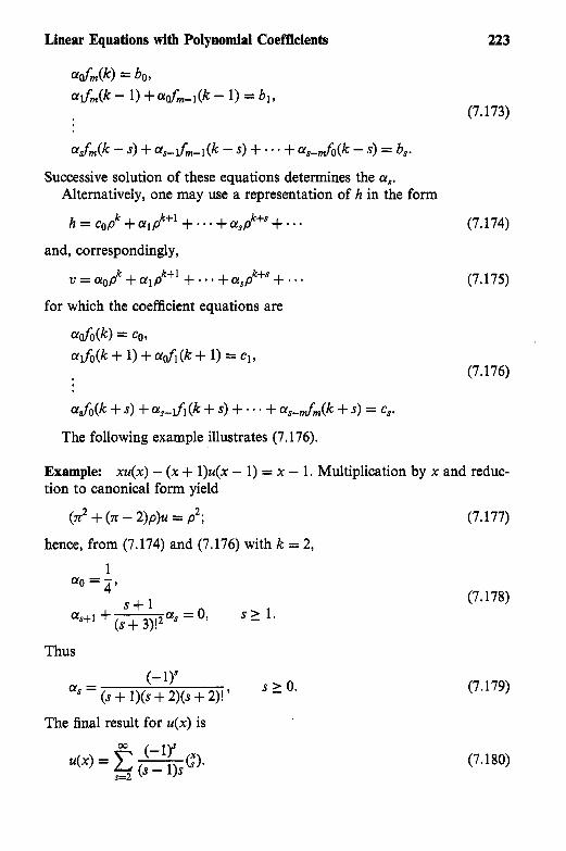
Linear Equations with Polynomial Coefficients
aafm(k) = bo, U&(k - 1) + Uafm-l(k - 1) = blv
aJm(k - S) + a,-dm-l(k - S) + * + ~J-mfo(k - S) = b,.
Successive solution of these equations determines the a,. Alternatively, one may use a representation of h in the form
223
(7.173)
and, correspondingly,
v=aop + a l p & + ' + . . . + U , p & + s + . . . k (7.175)
for which the coefficient equations are
aafo(k) = CO, atfo(k + 1) + aafi(k + 1) = Cl,
(7.176)
ah(k + S) + c~,-tfl(k + S) + * + a,-Jm(k + S) = C,-
The following example illustrates (7.176).
Example: xu(x) - ( x + l)u(x - 1) = x - 1. Multiplication by x and reduc- tion to canonical form yield
(nZ + (IC - 2)p)u = pz;
hence, from (7.174) and (7.176) with k = 2,
1 (110 = - 4 '
s + l a,+] + -a, = 0, S L 1. (S + 3)!2
Thus
(- 1Y S 2 0.
a, = (S + l)(s + 2)(s + 2)! '
The final result for u(x) is
(7.177)
(7.178)
(7.179)
(7.180)
" .... .. . , , ., . .. , ..... . .,. ._ ., . .. . .. , .. . . . . . . , . , . .." .. , . . . .

224 Chapter 7
Since the equation is of first order, the method of (5.33) may be used. For
u(x) = (x + l)t(x) (7.181)
this assume
because x + 1 is the solution of the homogeneous equation. This yields
= i ( Z + l)(z + 2) Az z
and hence a particular solution is u(x) = 1 + ( x + l)+(x + 2).
(7.182)
(7.183)
Lagrange's "variation of parameters" method [8] generalizes the second procedure of the previous example to equations of higher order when the complete solution of the homogeneous equation is known. Let wl(x), . . . , W&) constitute a fundamental system for the nth order equation LW = 0; to solve Lu = g, set
u(x) = A1 (x)q (x) + * * + A,(x)w,(x) (7.184) with the functions Al(x), .., &(x) to be determined. One has
Au(x) = Al(x)Awl(x) + I - + A,(x)Aw,(x) (7.185)
A condition will now be imposed on the functions A,(x) (1 I i 5 n) in order to simplify the form of u(x), namely
+ w1(X + l)AA,(X) + * * + wn(X + l)AA,(X).
VI(X + l)AAl(x) + * 0 + v,(x)AA,(x) = 0. (7.186)
(7.187) that is, precisely the same form it would have were the Ai(x) constant. Similarly, one has
A2u(x) = A1(X)A2V1(X) + + A,(x)A'w,(x) (7.188) with the condition
AVl(X + l)AAl(x) + * + Aw,(x)AA,(x) = 0. (7.189)
Proceeding in this manner, one calculates all differences up to A""u(x). Now let the original difference equation (7.1) be written in terms of u(x), Au(x), , A"u(x), then the equation Lu = g yields the last condition, namely
Afl-'W1(x + l)AAl(x) + + A""w,(x)AA,(x) = - (7.190) a, ( 4

Linear Equations with Polynomial Coefficients 225
The preceding system of equations determines AAl(x), - A&). One may now write a particular solution of Lu = g in the form
u(x) = &q(x)AAl(z) + + w,(x)AA,(z)]Az. (7.191) C
As a simple illustration consider the following:
Example: u(x + 2) - 5u(x + 1) + 6u(x) = g(x). A fundamental system is q ( x ) = 2', ~ ( x ) = 3'; hence one has
whose solution is
(7.192)
(7.193)
Thus a particular solution for u(x) is
u(x) = - 2x-z"]g(~)Az. (7.194) C
Setting c = 00, one has the form W
u(x) = - c (34-1 - 2-j-')g(x + j ) j = O
(7.195)
which, using (6.75), is convergent if lim suplg(x +j)l l"< 2. It may be noted that this is the same solution ond%%uld obtain using Broggi's method (6.71).
To provide a further illustration, the example of (7.6) will now be completed. From (7.7), (7.15) a fundamental system for (7.6) is q ( x ) = 3', Q ( X ) = X ; thus,
u(x) = 3'Al(X) + X A Z ( X ) . (7.196)
The pair of equations
3'+'AAl(x) + ( X + l)AAz(x) = 0,
has the solution
(7.197)

226
AAl(X) = 7 x + 3-x-'g(x), 4x "1
1 4x2 - l A.A~(x) = -- g w
Thus a particular solution for u(x)is
#(X) = i[3"(Z + 1) - x] - g(z) Az.
u(x) = - c [3-+'(x + j + 1) - x]
C 422 - 1 Again setting c = cc yields
W g(x +j) 0 4(x +jl2 - 1'
which is convergent for lim suplg(x + j)( l''< 1. j+ W
Chapter 7
(7.198)
(7.199)
(7.200)
7. THE LCFS M/M/C QUEUE WITH RENEGING- INTRODUCTION
In many teletraffic applications a good model for the delay experienced from the time of request for a line until a dial tone is received is the last come, first served queue in which a customer is allowed to renege before receiving the dial tone. This is the LCFS queue. This queue will be studied under the condition that all C servers are busy and the queue is in equilibrium. The formulations and solution will provide a good illustration of the methods of this chapter. It will be assumed that the arrival stream is Poisson with rate h (there is no restriction on h) and that the service distribution is exponential with C identical, independent servers. The total service rate over all servers is taken to be unity. These assumptions permit the use of a birth-death model for the problem formulation.
The concept of a test customer has been found useful in the analysis. A test customer in this investigation is one who arrives to find all servers busy, does not receive service, and cannot renege. The complementary waiting time distribution for such a customer who just arrived is designated uo(t). Test customers who are already waiting are ranked in accordance with the number of customers who will receive service ahead of them; u,(c) designates the complementary waiting time distribution of a test customer who must wait for n other customers to be served. Following Riordan [44], a differ- ential-difference equation will be formulated for v,(c). Using Laplace trans- formation, a difference equation for the Laplace transform, ;,(S), is obtained. The following three quantities for actual customers may be related to v,(t) : w,(c), complementary waiting time distribution; ~ ~ ( t ) , complemen-

Linear Equations with Polynomial Coefficients 227
tary waiting distribution of the customers who receive service; and r,(t), complementary waiting time distribution of those who renege. The subscript n has the same meaning as for v,(t), so that wo(t), so(& ro(t) refer to the actual customer who just arrived. It is assumed that the reneging propensity is exponential with rate a.
It is clear that w,(t) is related to w,(t) by
w,(t) = e%,(t), (7.201)
and hence
+,(S) = ;,(S + a). (7.202)
Since -e-"dw,(t) means the test customer starts (but does not receive) ser- vice and the actual customer does not renege, one has
(7.203)
and, in terms of Laplace transforms,
(7.204)
Also, since ae-"w,(t) dt means the test customer has not yet reached the server while the actual customer reneges at t , one has
r,(t) = lw e-Oxv,(x) dx/ e-axvn(x) dx,
and, accordingly,
(7.205)
(7.206)
Let V,, W,,, S,, R,, designate the corresponding mean values; then the values of the transforms for S -+ O+ provide the following:
V, = i,(O+), W, = cn(a)t
c,(.) + ac;(a) 1 -a;&) ' S, =
(7.207)
R, = -5k(a)/Cfl(a)
in which the prime indicates differentiation with respect to S at S = a. One may note the following relation obtained from (7.207):
(1 -aWn)Sfl +aW,R, = W,, (7.208)

228 Chapter 7
which may be compared with the similar relation in Ref. 40 for the first come, first served system with reneging. The quantity Q WO is simply the probability of reneging.
8. FORMULATION AND SOLUTION
For the birth-death formulation, the system is assumed to be in state n, that is, the test customer finds n ahead in the line at time t; the balance equations are obtained by considering the net changes in the time interval ( t , t + dt), thus
w,(t + dt) = (1 + an)dtw,-l(t) + (1 - (1 + A + an)dt)w,(t)
wo(t + dt) = (1 - (1 + A)dt)w,(t) + AdtWl(t). + m J , , l ( t ) , n 2 1, (7.209)
Accordingly, the differential-difference equation system obtained is
(7.210)
Since all servers are busy, one has w,(O+) = 1. Taking the Laplace transform of the system in (7.210), the following system satisfied by C&) is obtained:
Ai&) - (1 + A + S - Q + an)??,-] (S)
Aij1(S) - (1 + A + S)Co(S) = -1. + (1 - Q + an)C,&) = -1, n 2 2, (7.21 1)
It will be useful to consider the independent variable n to be continuous and to make the substitution
(7.212)
in which explicit indication of S is not needed at this point. Thus, from (7.211), one has
Au(x) - (A + S - Q + ax)u(x - 1) + Q(X - l)u(x - 2) = -1. (7.213)
Multiplying this equation by x and reducing to operational form, one obtains
Lu = (An - (S - a + .n)p)u = -p. (7.214)

Linear Equations with Polynomial Coefficients 229
To obtain a particular solution, one may use the method described in (7.174), but here advantage will be taken of the special form of L. An operator of the form
L =fob) +h (4P" (7.21 5 )
fo(n)x(n) +fm(n)xb - 46 (7.216)
is called binomial of order m [8]. The substitution U = x(n)w leads to
from which ~ ( n ) may be determined to effect a simplification of the opera- tor; for example, by .requiring the algebraic relation
(7.217)
u = r n + W ( 3 (7.218) in (7.214), one obtains
This equation is of first order with solution
hence,
From
(7.219)
(7.220)
(7.221)
(7.222)
the evaluation of the operator r(n + S/@) is immediate and the particular solution
(7.223)
is obtained. It may be noted that the assumption Cr=oampk+m for u(x) would simply lead one back to (7.223).
To obtain the second solution an expansion in inverse factorials C,"==,ampk-m will be assumed; as will be seen, this is particularly relevant

230 Chapter 7
because the final solution of (7.211) is to be a Laplace transform. The indicia1 equation yields k = -s/a. The recursion for the coefficients is
Am+s/a Q,+] =--
a m + 1 am* m L 0.
Using the Pochhammer notation [l81 for the ascending factorial r(n + a)
( 4 = r(a) = a ( a + l ) * . * ( a + n - l ) , n 2 1, = l , n = 0 ,
(7.224)
(7.225)
the solution in inverse factorials is
U ( X ) = D (s/a)m (A/aIm (7.226) ( x + 1 + s/a), m!
Since the confluent hypergeometric function [24], #(a, b; x) , is defined by
(7.227)
u(x) takes the form
U ( X ) = D r(x + 1) a a
The complete solution of (7.213) is, by (7.223) and (7.228),
(7.228)
(7.229a)
Since ij#(oo) = 0, one must have C = 0; accordingly, u(x) simplifies to
(7.229b)
One may now revert back to the original variables, n, and ijn(s) through n = x - l/cr to obtain
(7.230a)
In order to determine D, the same method that was used in (6.25) for the solution of the M/M/1 queue will be used. The validity of the difference

Linear Equations with Polynomial Coefficients 231
equation (7.21 1) will be extended to include the boundary condition, Setting n = 1 in (7.21 l), one has
ACl(S) - (1 + A +s)Co(s) + C-l(S) = -1. (7.230b)
Subtracting the boundary equation from this provides the extension condi- tion <-,(S) 0. One now determines D from this condition applied to (7.230) with n = -1; thus,
(7.23 1)
The solution for C&) after simplifying the gamma function expressions is, accordingly,
1 +-;-) S s + l A *
s + l A
C&) = - - - a a
a a
In particular for n = 0,in (7.232), one obtains
(7.232)
(7.233)
' 'a' a 'a' In many applications of this model, the parameter a is small, a possible
set of values is A = 1.1, a = ,0025. The solution of (7.233) is not well suited for computation for such values. Thus it is important to obtain another solution of the system suitable for small a. This will be done by constructing a perturbation solution in a of (7.21 1). Since a appears as a polynomial in (7.21 1) only in the coefficients of ijnWl(s), C,,-&), a power series solution in a exists; thus, one may write
W
C&) = c Cll"'(s)ak. (7.234) k=O
On1 +:')(S), Cf)(s) will be determined. Replacing ;,,(S) in (7.21 1) by Cio)(s) + aC$' r (S) and equating corresponding coefficients of ak on both sides of the equation, the system obtained for C$o)(s) is
A C p - (1 + A +s)C;!l + = -1,
A i j p - (1 + A + s)Cp = -1. (7.235)

232 Chapter 7
This is an equation with constant coefficients. A particular solution is l/s. The characteristic equation has the roots
Thus the general solution of the equation is
1 <io) = - + Cpy + Dpi. (7.237) S
Because ;,(W) = 0, one must have D = 0 and
- 1 v, = - + cpy. (7.238) S
Extending the boundary condition to negative n, rovides the condition i i l(s) 0 and hence C = - p l / s . The solution for p ) is, accordingly,
(7.239)
This solution corresponds to the case of no reneging and has already been obtained [44]. In this case one must have 31 < 1 to ensure an equilibrium condition; however, in the perturbation solution being developed as an approximation to the reneging case, no restriction on 31 need be imposed.
The system of equations for $)(S) is
A$) - (1 + h + + = (n - - (7.240) 31p - (1 + h + S)?#) = 0.
Using the result of (7.239) in (7.240) yields
(7.241)
A particular solution is obtained operationally as follows:
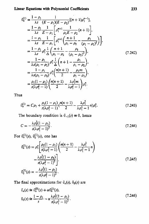
Linear Equations with Polynomial Coefficients 233
Thus
5 p = Cp1 + The boundary condition is kl(s) 0, hence
C = - A P W - P11 @p' - 1)2 '
For .i;il)(s), #)(S), one has
The final approximations for C&), C&) are
igs) G! i p ( S ) + a#) (s) ,
C&) E - - 1 - P1 (;yAP:(l - P11 S s(Ap? - '
(7.242)
(7.243)
(7.244)
(7.245)
(7.246)
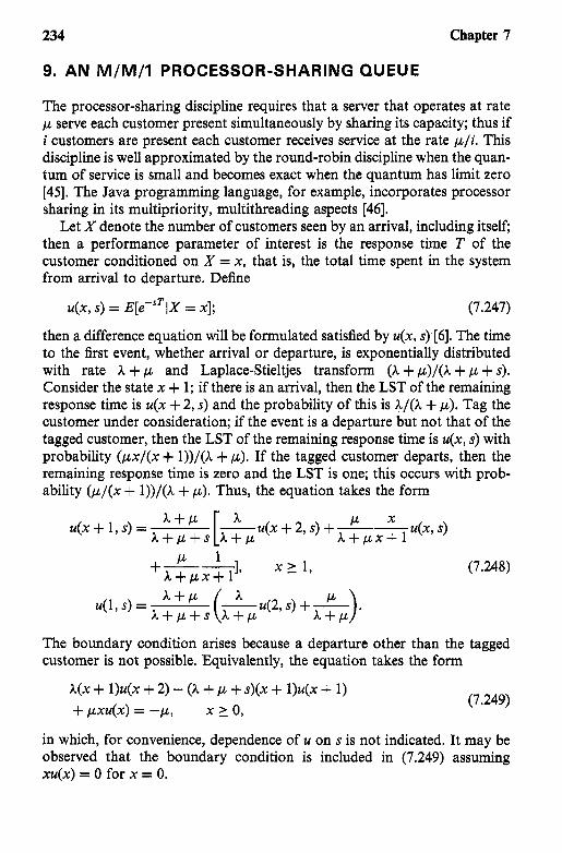
234 Chapter 7
9. AN M/M/I PROCESSOR-SHARING QUEUE
The processor-sharing discipline requires that a server that operates at rate p serve each customer present simultaneously by sharing its capacity; thus if i customers are present each customer receives service at the rate p/i . This discipline is well approximated by the round-robin discipline when the quan- tum of service is small and becomes exact when the quantum has limit zero [45]. The Java programming language, for example, incorporates processor sharing in its multipriority, multithreading aspects [46].
Let X denote the number of customers seen by an arrival, including itself; then a performance parameter of interest is the response time T of the customer conditioned on X = x, that is, the total time spent in the system from arrival to departure. Define
u(x, S) = E[e-STIX = x]; (7.247)
then a difference equation will be formulated satisfied by u(x, S) [6]. The time to the first event, whether arrival or departure, is exponentially distributed with rate h + p and Laplace-Stieltjes transform (h + p)/@ + p + S).
Consider the state x + 1; if there is an arrival, then the LST of the remaining response time is u(x + 2, S) and the probability of this is h/(h + p). Tag the customer under consideration; if the event is a departure but not that of the tagged customer, then the LST of the remaining response time is u(x, S) with probability ( p x / ( x + l))/@ + p). If the tagged customer departs, then the remaining response time is zero and the LST is one; this occurs with prob- ability (p /@ + l))/@ + p). Thus, the equation takes the form
u(x+ 1,s) = u(x + 2, S) +-- h + p x + 1 u(x, S)
P X
+- P 1 h+pUx+l -1, x 1 1 , (7.248)
u(1, S) = h + p + s h + p F h + p h + P > *
u(2, S) + - The boundary condition arises because a departure other than the tagged customer is not possible. Equivalently, the equation takes the form
h(x + l)u(x + 2) - (h + p + s)(x + l)u(x + 1) + pxu(x) = -p, x L 0,
(7.249)
in which, for convenience, dependence of u on S is not indicated. It may be observed that the boundary condition is included in (7.249) assuming xu(x) = 0 for x = 0.

Linear Equations with Polynomial Coefficients 235
Equation (7.249) degenerates to first order when h = 0. Thus one may think of the two-dimensional manifold of solutions as consisting of the union of two one-dimensional manifolds in which one manifold consists of functions regular in h at h = 0 and the other not. Since it may be assumed that the processor-sharing model is meaningful in the neighborhood of h = 0, one may assume a solution of the form
bo
u(x) = c uj(x)k; j=O
(7.250)
that is, one may assume the required solution is regular. This is called a singular perturbation expansion [7]. Substitution of (7.250) into (7.249) yields the following system of first-order equations:
- 1 (x + l)uo(x + 1) - (1 + ;)-lxuo(x) = ( 1 + ;) 7
uo(1) = (1 +;)-l,
(7.251)
in which A operates with respect to x. The solution of this infinite system is
Since
the termwise inversion of (7.250) is easily accomplished. Define
F(t, x) = P[T > tlX = x] + 1 - u(x, S),
(7.253)
(7.254)
. . . .. . _* ,,. , ... ., .. ... .. .. , . ,. . . ....... ... - I .., . _._....-.-.... "^. .,_,.,. u.,,uI,L- ...-.. *e..---. - -
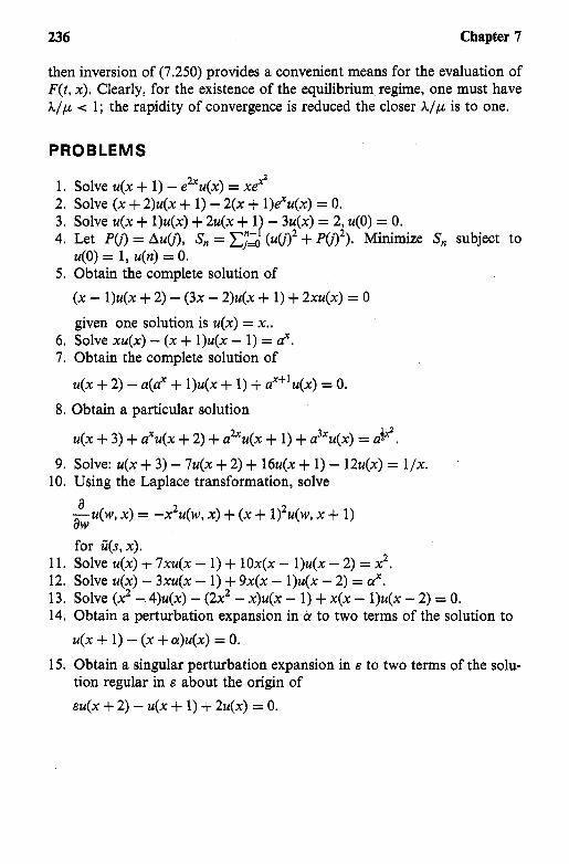
236 Chapter 7
then inversion of (7.250) provides a convenient means for the ,evaluation of F( t , x). Clearly, for the existence of the equilibrium, regime, one must have A/ ,u 1 ; the rapidity of convergence is reduced the closer A / p is to one.
PROBLEMS
I . Solve u(x + 1 ) - e2xu(x) = xex2 2. Solve ( x + 2)u(x + 1 ) - 2(x + l)e"u(x) = 0. 3. Solve u(x + l)u(x) + 2u(x + l ) - 3$x) = 2, u(0) = 0. 4. Let PO) = Au(j), S, = (u(j) + P(j)'>. Minimize S, subject to
5. Obtain the complete solution of u(0) = 1 , u(n) = 0.
( x - l)u(x + 2) - (3x - 2)u(x + 1 ) + 2xu(x) = 0
given one solution is u(x) = x.. 6 . Solve xu(x) - ( x + l)u(x - 1 ) = 2. 7. Obtain the complete solution of
u(x + 2) - a ( 2 + l)u(x + 1 ) + d + ' U ( X ) = 0.
u(x + 3) + aXu(x + 2) + aZXu(x + 1 ) + a3xu(x) = aix2.
8. Obtain a particular solution
9. Solve: u(x + 3) - 7u(x + 2) + 16u(x + 1 ) - 12u(x) = l /x . 10. Using the Laplace transformation, solve
--u(w, x ) = -x2u(w, x ) + ( x + l)'u(w, x + 1 ) a aw for ii(s, x).
1 1. Solve u(x> + 7xu(x - I ) + 1Ox(x - l)u(x - 2) = X'. 12. Solve u(x) - 3xu(x - 1) + 9x(x - l)u(x - 2) = ax. 13. Solve (x2 -. 4)u(x) - (2x2 - x)u(x - 1 ) + x(x - l)u(x - 2) = 0. 14. Obtain a perturbation expansion in.& to two terms of the solution to
u(x + 1 ) - ( x + Q ) U ( X ) = 0.
15. Obtain a singular perturbation expansion in E to two terms of the solu- tion regular in E about the origin of EU(X + 2) - U ( X + 1 ) + 2 U ( X ) = 0.

References
1. RP Boas Jr. Entire Functions. New York: Academic Press, 1954.
2. NI Achiezer. Theory of Approximation. New York: Frederick Ungar, 1956.
3. C Truesdell. A Unified Theory of Special Functions. Annals of Mathematics Studies No. 18. Princeton, NJ: Princeton University Press, 1948.
4. W Gruber, H Knapp. Contributions to the Method of Lie Series, Mannheim: Hochschultaschenbiicher-Verlag, 1967.
5 . EJ Watson. Laplace Transforms and Applications. Van Nostrand Reinhold, 1924.
6. B Sengupta, DL Jagerman. A conditional response time of the M/M/l proces- sor-sharing queue. BSTJ 64:409421, 1985.
7. B Sengupta. A perturbation method for solving some queues with processor sharing discipline. J Appl Prob 26:209-214, 1989.
8. LM Milne-Thomson. The Calcululs of Finite Differences. London: Macmillan, 1933.
9. C Jordan. Calculus of Finite Differences. New York: Chelsea, 1947.
10. G Doetsch. Theorie und Anwendung der Laplace-Transformation. New York: Dover, 1943.
237

References
1 1. DV Widder. The Laplace Transform. Princeton, NJ: Princeton University Press, 1941.
12. NTJ Bailey. The Elements of Stochastic Processes. New York: Wiley, 1964.
13. TE Harris. Theory of Branching Processes. New York: Springer, 1963.
14. MS Bartlett. An Introduction to Stochastic Processes. Cambridge: University Press, 1956.
15. T Fort. Finite Differences and Difference Equations in the Real Domain. Oxford: Oxford University Press, 1948.
26. R Bellman. Dynamic Programming. Princeton, NJ: Princeton University Press, 1957.
17. NE Norlund. Vorlesungen iiber Differencenrechnung. Berlin: Springer Verlag, 1924.
18. Bateman Project. Higher Transcendental Functions. New York: McGraw-Hill, 1953.
19. Hardy, Littlewood, Polya. Inequalities. Cambridge: University Press, 1959.
20. J F Steffensen. Interpolation. New York: Chelsea, 1950.
21. K Knopp. Theory and Application of Infinite Series. London: Blackie & Son, 1946.
22. VI Krylov. Approximate Calculation of Integrals. New York: Macmillan, 1962.
23. NK Bary. A Treatise on Trigonometric Series. New York: Pergamon, 1964.
24. W Magnus, F Oberhettinger. Formulas and Theorems for the Functions of Mathematical Physics. New York: Chelsea, 1954.
25. TJI’A Bromwich. An Introduction to the Theory of Infinite Series, London: Macmillan, 1908.
26. RB Cooper. Introduction to Queueing Theory. New York: North Holland, 1981.
27. L Kosten. Stochastic Theory of Service Systems. New York: Pergamon, 1973.
28. DL Jagerman. Methods in traffic calculations. AT&T Bell Lab Tech J 63(7): 1984.
29. DL Jagerman. “Some Properties of the Erlang Loss Function,” BSTJ 53(3): 1974.
30. L Taka’cs. Introduction to the Theory of Queues. Annals of Mathematics Studies No. 18. Princeton, NJ: Princeton University Press, 1948.

References 239
31. H Akimaru, T Nishimura. The derivatives of Erlang's B formula. Rev Elec Commun Lab ll(9-10): 1963.
32. RF Rey. Engineering and Operating in the Bell System. 2nd ed. Murray Hill, NJ: ATLT Bell Laboratories, 1983.
33. DR Cox. Renewal Theory. New York: Methuen, 1962.
34. RE Mickens. Difference Equations. Van Nostrand Reinhold, 1987.
35. S Karlin and HM Taylor. A First Course in Stochastic Processes. New York: Academic Press, 1975.
36. PL Butzer, H Berens. Semi-Groups of Operators and Approximation. New York: Springer-Verlag, 1967.
37. GH Hardy. Divergent Series. Oxford: Clarendon Press, 1949.
38. R Askey. Ramanujan's Extensions of the Gamma and Beta Functions.
39. ND de Bruijn. Asymptotic Methods in Analysis. Amsterdam: North Holland, 1958.
40. TL Saaty. Modern Nonlinear Equations. New York: Dover, 1981.
41. DL Jagerman. An inversion technique for the Laplace transform with applica- tion to approximation. BSTJ 57(3): 1978.
42. DL Jagerman. An inversion technique for the Laplace transform. BSTJ 61(8): 1982.
43. G Boole. A Treatise on the Calculus of Finite Differences. Stechert, 1931.
44. J Riordan. Stochastic Service Systems. New York: Wiley, 1962.
45. L Kleinrock. Queuing Systems. Vol 2. Computer Applications. New York: Wiley Interscience, 1976.
46. K Jamsa. Java Now! Las Vegas, NV: Jamsa Press, 1996.
, , , ,.,, , . , ,, ,,, , _... , , , , ,,". , . . . . ._ ..._... .. , ... , . . . .. . . , .. ... I I .... " ..... .... ,... . . . . , . . .. .. "...


Index
A
Alternate representation of sum, 89 Approximation to generators, 161 Approximation method, 176
approximate inversion, 176 approximation to P(t,O), 177
Approximation to solution, 114 error estimate, 114
B
Bandlimited functions, 105 samples on half line, 105
Bernoulli’s polynomials, 50 Bernoulli numbers, 5 1 complementary argument
generating function, 54 generating function for Bernoulli
multiplication theorem, 53 problem of Bernoulli, 51
theorem, 54
numbers, 55
[Bernoulli polynomials] relation to zeta function, 55 table of Bernoulli numbers, 53 table of Bernoulli polynomials, 52
Beta function, 7 Birth-death model, 137
solution, 138 Bound for remainder, 83 Branching process approximation, 145
critical case, 146 nonnegative variable, 146 subcritical case, 146 supercritical case, 145
Branching processes, 1.36 generator for population, 137
C
Casorati’s determinant, 202 Casorati’s theorem, 26
equation, 29 construction of a difference

242 Index
Class of linear transformations, 89 associated function, 90 Bore1 transform, 90 exponential order of sequence, 89 maximum modulus, 90 vector space, 90
Coefficients A,(@), 127 Complete equation, 222 Constant coefficients, 172
characteristic equation, 173 homogeneous equation, 173 multiple roots, 173 simple roots, 173
Convergence of infinite products, 1 13 Convolution integral representation,
101 derived error bound, 102 error estimate theorem, 102
Critical points, 143 classification, 144
D
Depression of order, 201 Derivative, 129
approximate mean work in
approximation for Erlang loss
approximation to u’(x)/u(x), 130
M/G/l, 131
function, 130
Differential-difference equations,
examples of F-equation, 124 method of Truesdell, 122 reduction procedure, 123
Differentiation, 39 Differentiation formula, 8 1
122
asymptotic properties, 97. 82 mth derivative of sum, 82
E
Equation of nth order, 158
[Equation of nth order]
Equations reducible to constant coefficients, 188
Erlang loss function, 161 Error bound for transformation,
examples, 158
101 derived error bound, 102 error transformation, 101
Euler equation, 25 Euler summability, 159
application of summability,
circle of summability, 160 consistency, 160 regularity, 160
periodic Bernoullian functions,
usual form of expansion, 76 Exact expansion for P(t,O), 177 Exceptional cases, 217
multiple roots, 217 multiple roots - Newton series,
161
Euler-Maclaurin expansion, 75
75
219 Existence of principal’ sum, 77 Expansion for g(z), 142
approximation to g(z), 143 Expansions and functional
equations, 96
97 differential-difference equation,
first order difference equation, 98 Newton’s expansion, 96
F Factorial function, 4 Factorial series, 7
first kind, 7 second kind, 7 uniqueness, 9

Index 243
Finite source model, 195 Functional equations, 132
G
Gauss-Laguerre quadrature table, 6 1 Gauss-Legendre quadrature table,
General operational solution,
inverse factorial series, 212 reduction to canonical form, 211 use of R, 213
Clairault, 22 geometric distribution, 22 Poisson distribution, 22 Riccati, 22 two parameter family, 23
GI/M/1 queue, 125 Gregory-Laplace quadrature,
161
210
Genesis, 21
64
H
Haldane’s method, 149
Heymann’s theorem, 29 Homogeneous equation of order n,
expansion for l/g(z), 150
25 congruent points, 26 fundamental system, 26 general form of solution, 29
bounds for eigenvalue and sum,
commutability, 45 convexity of eigenvalue, 47 derivative, 44 difference, 44 eigenfunction of homogeneous
sum, 45 extension of summability, 45
Homogeneous form, 44
46
[Homogeneous form] representation of Laplace
Homogeneous sum exponential transforms, 45
weight, 100
1
Identity in z, 207 Indicia1 equation, Inverse factorial
Inhomogeneous equation, 179, series, 213
114 Boole’s operational method, 179 concomitant boundary condition,
construction of solution, 114 method of Broggi, 182 partial fraction method, 182 specification of u(O), 116 useful form of solution, 115
Inhomogeneous form, 197 Integral equations, 102
inhomogeneous, 104 Invariant function, 157 Inverse of z + m, 206
115
1
Lagrange’s method, 190 Lagrange’s variation of parameters,
Landau, 7 224
associated series, 7 convergence, 7
Laplace numbers generating function, 63
Laplace, 12 abscissa, 13 bilateral, 13 convergence, 12 convolution, 13 operational properties, 14

244 Index
[Laplace]
Laplace numbers, 62
Laplace’s method, 183 Laplace’s observation, 193
Boole’s example, 194 LCFS M/M/C queue with reneging,
transform, 12
Laplace numbers table, 63
226 final solution, 231 formulation and solution, 228 method for binomial equations,
perturbation solution for small
second solution, 229 test customer, 226
229
alpha, 231
Level crossings of work, 120 Linear homogeneous equation, 110
gamma function, 11 1 infinite product solution, 1 13 multiplication formula, 11 1 solution in terms of gamma
function, 1 12 Linear transformation, 91
class A, 91 eigenfunction, 93 generating function, 91 inverse, 94 sum and product, 93
Lower bound theorem, 49
M
M/G/l queue with reneging, 121 difference equation, 121 M/M/1 case, 122 Volterra integral equation, 121
differential-difference equation,
semigroup type, 24
M/M/l delay model, 24
24
M/M/l processor sharing queue,
singular perturbation solution,
tagged customers, 234
234
235
M/M/ 1 queue transient solution, 174
exact inversion, 176 Laplace transform of solution,
M/M/l queue with feedback, 132 M/M/C Erlang blocking model, 24 Mellin, 14
175
convolution, 14, 15 inverse factorial series, 14 operational properties, 14, 15 product of series, 16
Milne-Thomson, 30 asymptotic criterion, 30
Monomial equations in 5t, 207 multiple roots, 208
Monomial equations in p, 204 Erlang loss function, 204 use of factorial series, 204
N
Newton’s expansion, 2 defined, 2 uniqueness, 8
Nonlinear difference equation, 133 generating function g(zlh), 133 ordinary differential equation,
partial differential equation, 134 Norlund, 8
uniform convergence, 8 Norlund principal sum, 75 Norlund sum for complex
133
arguments, 99
formula, 100 complementary argument

Index 245
[Norlund sum for complex arguments]
complementary argument theorem, 100
expansion for, 99 integral representation, 99
asymptotic properties, 57 error estimate, 57 homogeneous sum, 59 representation of sum, 59
Null function, 13 Numerical differentiation, 60
Norlund’s expansion, 56
0
Operational formulae, 17
Operational method of Boole, 179
Operators, 1 Operator n, 205 Operators n and p, 203
shift formula, 17
P
Partial difference equations, 189 Bernoulli trials, 190 Pascal’s triangle, 189
Perturbation solution, 147 Norlund sum expression, 147 perturbation solution, 148
Principal solution, 33 limits and span, 33 Norlund definition, 33 sum, 33
Properties of sum, 34 limiting form, 36 linear change of variable, 34 multiplication theorem, 35 span integral, 35 sum from primitive, 36
Psi-function, 10
Q Quadrature formula for sum, 62 Quadrature of homogeneous sum,
65
weight, 66 coefficients for exponential
coefficients for linear weight, 68 Queueing model M/M/n, 118
asymptotic expansion, 120 differences of l/B(O,a), 120 Erlang loss function, 118 expansion for l/B(x,a), 119 extension to continuous
argument, 1 19 Fortet integral, 120
R
Reduction of order, 21 3 Repeated summation, 40 Representation theorem, 90 Riccati form, 135
inifinitesimal generators, 136 solution, 135
Roots differing by an integer, 220
5
Separation of variables, 191 Sequence of transformations, 11 1
convergence of generating
convergence theorem, 95 functions, 95
Shift formula, 205 Simultaneous first-order equations,
154 equivalent differential equations,
154 equivalent partial differential
equations, 154 limiting form, 157

246 Index
[Simultaneous first-order equations] Newton’s expansion, 156 partial differences, 156 U-operator method, 155
Solution in Newton series, 215 descending factorials, 216 example - integral form of
indicia1 equation, 21 5 Solution of functional equation, 152
example, 153 example of M/M/l queue with
solution of special case, 153
solution, 2 16
feedback, 152
Stirling equation, 192 Stirling numbers, 4
first kind, 5 second kind, 5
Sum of Laplace transforms, 41 representation theorem, 41
Summability, 39 Summation by parts, 38 Summation of series, 11
from sum of function, 37
T
Taylor’s series, 3 Time-homogeneous model, 25
Trigonometric expansions, 84 coefficients for, 85 example of, 86 +-function example, 87 removal of discontinuity, 87 sum of exponential, 86
U Uniqueness theorem, 92 U-operator solution, 138
accuracy dependent on h, 141 Hille’s representation, 140 infinitesimal generator, 140 invariant function, 141 modification for good accuracy,
Newton’s series expansion, 139 reduction to Lie-Grobner
relation to semigroups, 140 Use of Laplace transform, 184
example, 186 principal solution, 184
141
operator, 139
v Volterra integral equation, 65