Embed Size (px)
Citation preview

Functional Equations of L-Functions for Symmetric Products
of the Kloosterman Sheaf ∗
Lei FuInstitute of Mathematics, Nankai University, Tianjin, P. R. China
Daqing WanDepartment of Mathematics, University of California, Irvine, CA 92697
Abstract
We determine the (arithmetic) local monodromy at 0 and at ∞ of the Kloosterman sheafusing local Fourier transformations and Laumon’s stationary phase principle. We then cal-culate ǫ-factors for symmetric products of the Kloosterman sheaf. Using Laumon’s productformula, we get functional equations of L-functions for these symmetric products, and provea conjecture of Evans on signs of constants of functional equations.
Key words: Kloosterman sheaf, ǫ-factor, ℓ-adic Fourier transformation.
Mathematics Subject Classification: 11L05, 14G15.
Introduction
Let p 6= 2 be a prime number and let Fp be the finite field with p elements. Fix an algebraic
closure F of Fp. Denote the projective line over Fp by P1. For any power q of p, let Fq be the finite
subfield of F with q elements. Let ℓ be a prime number different from p. Fix a nontrivial additive
character ψ : Fp → Q∗ℓ . For any x ∈ F∗
q , we define the one variable Kloosterman sum by
Kl2(Fq, x) =∑
x∈F∗
q
ψ(
TrFq/Fp
(
λ +x
λ
))
.
In [3], Deligne constructs a lisse Ql-sheaf Kl2 of rank 2 on Gm = P1 − {0,∞}, which we call the
Kloosterman sheaf, such that for any x ∈ Gm(Fq) = F∗q , we have
Tr(Fx,Kl2,x) = −Kl2(Fq, x),
∗The research of Lei Fu is supported by the NSFC (10525107).
1

where Fx is the geometric Frobenius element at the point x. For a positive integer k, the L-function
L(Gm,Symk(Kl2), T ) of the k-th symmetric product of Kl2 was first studied by Robba [15] via
Dwork’s p-adic methods. Motivated by applications in coding theory, by connections with modular
forms, p-adic modular forms and Dwork’s unit root zeta functions, there has been a great deal of
recent interests to understand L(Gm,Symk(Kl2), T ) as much as possible for all k and for all p.
This quickly raises a large number of interesting new problems.
Let j : Gm → P1 be the inclusion. We shall be interested in the L-function
Mk(p, T ) := L(P1, j∗(Symk(Kl2)), T ).
This is the non-trivial factor of L(Gm,Symk(Kl2), T ). The trivial factor of L(Gm,Symk(Kl2), T )
was completely determined in Fu-Wan [6]. By general theory of Grothendieck-Deligne, the non-
trivial factor Mk(p, T ) is a polynomial in T with integer coefficients, pure of weight k + 1. Its
degree δk(p) can be easily extracted from Fu-Wan [7] Proposition 2.3, Lemmas 4.1 and 4.2:
δk(p) =
k−12 −
[
k2p + 1
2
]
if k is odd,
2(
[k−24 ] − [ k
2p ])
if k is even.
For fixed k, the variation of Mk(p, T ) as p varies should be explained by an automorphic form,
see Choi-Evans [2] and Evans [4] for the precise relations in the cases k ≤ 7 and Fu-Wan [8] for a
motivic interpretation for all k. For k ≤ 4, the degree δk(p) ≤ 1 and Mk(p, T ) can be determined
easily. For k = 5, the degree δ5(p) = 2 for p > 5. The quadratic polynomial M5(p, T ) is explained
by an explicit modular form [14]. For k = 6, the degree δ6(p) = 2 for p > 6. The quadratic
polynomial M6(p, T ) is again explained by an explicit modular form [9]. For k = 7, the degree
δ7(p) = 3 for p > 7. The cubic polynomial M7(p, T ) is conjecturally explained in a more subtle way
by an explicit modular form in Evans [4]. We will return to this conjecture later in the introduction.
For fixed p, the variation of Mk(p, T ) as k varies p-adically should be related to p-adic auto-
morphic forms and p-adic L-functions. No progress has been made along this direction. The p-adic
limit of Mk(p, T ) as k varies p-adically links to an important example of Dwork’s unit root zeta
function, see the introduction in Wan [18]. The polynomial Mk(p, T ) can be used to determine the
weight distribution of certain codes, see Moisio [12][13], and this has been studied extensively for
small p and small k. The p-adic Newton polygon (the p-adic slopes) of Mk(p, T ) remains largely
mysterious.
2

By Katz [10] 4.1.11, we have (Kl2)∨ = Kl2 ⊗ Qℓ(1). So for any natural number k, we have
(Symk(Kl2))∨ = Symk(Kl2) ⊗ Qℓ(k).
General theory (confer [11] 3.1.1) shows that Mk(p, T ) satisfies the functional equation
Mk(p, T ) = cT δMk
(
p,1
pk+1T
)
,
where
c =
2∏
i=0
det(−F,Hi(P1F, j∗(Symk(Kl2)))
(−1)i+1
,
δ = −χ(P1F, j∗(Symk(Kl2)) = δk(p),
and F denotes the Frobenius correspondence. Applying the functional equation twice, we get
c2 = p(k+1)δ.
Based on numerical computation, Evans [4] suggests that the sign of c should be −(
p105
)
(the
Jacobi symbol) for k = 7, and −(
p1155
)
for k = 11. In this paper, we determine c for all k and all
p > 2. The main result of this paper is the following theorem.
Theorem 0.1. Let p > 2 be an odd prime. If k is even, we have
c = p(k+1)([ k−24 ]−[ k
2p]).
If k is odd, we have
c = (−1)k−12 +[ k
2p+ 1
2 ]pk+12 ( k−1
2 −[ k2p
+ 12 ])
(−2
p
)[ k2p
+ 12 ]
∏
j∈{0,1,...,[ k2 ]}, p6 |2j+1
(
(−1)j(2j + 1)
p
)
.
Corollary 0.2. If k is even and p > 2, the sign of c is always 1. If k is odd and p > k, the sign
of c is
(−1)k−12
∏
j∈{0,1,...,[ k2 ]}, p6 |2j+1
(
(−1)j(2j + 1)
p
)
.
In the above corollary, if we take k = 7, we see that the sign of c for p > 7 is
−(
1 · (−3) · 5 · (−7)
p
)
= −(
105
p
)
= −( p
105
)
;
if we take k = 11, we see that the sign of c for p > 11 is
−(
1 · (−3) · 5 · (−7) · 9 · (−11)
p
)
= −(−1155
p
)
= −( p
1155
)
,
3

consistent with Evans’ calculation.
In the case k = 7, Evans proposed a precise description of M7(p, T ) in terms of modular forms.
For k = 7 and p > 7, the polynomial M7(p, T ) has degree 3. Write
M7(p, T ) = 1 + apT + dpT2 + epT
3.
The functional equation and our sign determination show that one of the reciprocal roots for
M7(p, T ) is(
p105
)
p4 and ep = −(
p105
)
p12. Denote the other two reciprocal roots by λp and µp
which are Weil numbers of weight 8. We deduce that
ap = −(( p
105
)
p4 + λp + µp
)
, λpµp = p8, |λp| = |µp| = p4.
To explain the numerical calculation of Evans, Katz suggests that there exists a two dimensional
representation
ρ : Gal(Q/Q) → GL(Q2
ℓ)
unramified for p > 7 and a Dirichlet character χ such that
α2p = χ(p)
( p
105
) λp
p4,
β2p = χ(p)
( p
105
) µp
p4,
αpβp = χ(p),
where αp and βp are the eigenvalues of the geometric Frobenius element at p under ρ. We then
have
1 −( p
105
) ap
p4= 2 +
( p
105
) λp
p4+
( p
105
) µp
p4
= χ(p)(2αpβp + α2p + β2
p)
= χ(p)(αp + βp)2.
Set b(p) = p(αp + βp). Evans [4] conjectured that b(p) is the p-th Hecke eigenvalue for a weight 3
newform f on Γ0(525). Our ap equals −cpp2 in [4].
Our proof of Theorem 0.1 naturally splits into two parts, corresponding to the two ramification
points at 0 and ∞. Let t be the coordinate of A1 = P1 − {∞}. For any closed point x in P1, let
P1(x) be the henselization of P1 at x. By Laumon’s product formula [11] 3.2.1.1, we have
c = pk+1∏
x∈|P1|ǫ(P1
(x), j∗(Symk(Kl2))|P1(x)
, dt|P1(x)
),
4

where |P1| is the set of all closed points of P1. When x 6= 0,∞, the sheaf Symk(Kl2)|P1(x)
is lisse
and the order of dt at x is 0. So by [11] 3.1.5.4 (ii) and (v), we have
ǫ(P1(x), j∗(Symk(Kl2))|P1
(x), dt|P1
(x)) = 1
for x 6= 0,∞. Therefore
c = pk+1ǫ(P1(0), j∗(Symk(Kl2))|P1
(0), dt|P1
(0))ǫ(P1
(∞), j∗(Symk(Kl2))|P1(∞)
, dt|P1(∞)
).
In §1, we prove the following.
Proposition 0.3. We have
ǫ(P1(0), j∗(Symk(Kl2))|P1
(0), dt|P1
(0)) = (−1)kp
k(k+1)2 .
In §2, we prove the following.
Proposition 0.4. ǫ(P1(∞), j∗(Symk(Kl2))|P1
(∞), dt|P1
(∞)) equals
p−(k+1)( k+84 +[ k
2p])
if k = 2r for an even r,
p−(k+1)( k+64 +[ k
2p])
if k = 2r for an odd r, and
(−1)k+12 +[ k
p]−[ k
2p]p−
k+12 ( k+5
2 +[ kp]−[ k
2p])
(−2
p
)[ kp]−[ k
2p]
∏
j∈{0,1,...,[ k2 ]}, p6 |2j+1
(
(−1)j(2j + 1)
p
)
if k = 2r + 1.
We deduce from the above two propositions the constant c as stated in Theorem 0.1 using the
following facts:
[
k − 2
4
]
=
{
k−44 if k = 2r for an even r,
k−24 if k = 2r for an odd r,
[
k
p
]
−[
k
2p
]
=
[
k
2p+
1
2
]
if k is odd.
To get Proposition 0.4, we first have to determine the local (arithmetic) monodromy of Kl2
at ∞. This is Theorem 2.1 in §2, which is of interest itself, and is proved by using local Fourier
transformations and Laumon’s stationary phase principle.
5

1 Calculation of ǫ(P1(0), j∗(Symk(Kl2))|P1
(0), dt|P1
(0))
Let η0 be the generic point of P1(0), let η0 be a geometric point located at η0, and let V be an
Qℓ-representation of Gal(η0/η0). Suppose the inertia subgroup I0 of Gal(η0/η0) acts unipotently
on V . Consider the ℓ-adic part of the cyclotomic character
tℓ : I0 → Zℓ(1), σ 7→(
σ( ℓn√t)
ℓn√t
)
.
Note that for any σ in the inertia subgroup, the ℓn-th root of unity σ( ℓn√t)
ℓn√t
does not depends on
the choice of the ℓn-th root ℓn√t of t. Since I0 acts on V unipotently, there exists a nilpotent
homomorphism
N : V (1) → V
such that the action of σ ∈ I0 on V is given by exp(tℓ(σ).N). Fix a lifting F ∈ Gal(η0/η0) of the
geometric Frobenius element in Gal(F/Fp).
Lemma 1.1. Notation as above. Let V = Kl2,η0. There exists a basis {e0, e1} of V such that
F (e0) = e0, F (e1) = pe1
N(e0) = 0, N(e1) = e0.
Proof. This is the n = 2 case of Proposition 1.1 in [6].
Lemma 1.2. Keep the notation in Lemma 1.1. Let {f0, . . . , fk} be the basis of Symk(V ) =
Symk(Kl2,η0) defined by fi = 1
i!ek−i0 ei
1. We have
F (fi) = pifi, N(fi) = fi−1,
where we regard fi−1 as 0 if i = 0.
Proof. Use the fact that for any v1, . . . , vk ∈ V , we have the following identities in Symk(V ):
F (v1 · · · vk) = F (v1) · · ·F (vk),
N(v1 · · · vk) =k
∑
i=1
v1 · · · vi−1N(vi)vi+1 · · · vk.
6

Corollary 1.3. The sheaf Symk(Kl2)|η0has a filtration
0 = F−1 ⊂ F0 ⊂ · · · ⊂ Fk = Symk(Kl2)|η0
such that
Fi/Fi−1∼= Ql(−i)
for any i = 0, . . . , k.
Proof. This follows from Lemma 1.2 by taking Fi to be the sheaf on η0 corresponding to the galois
representation Span(f0, . . . , fi) of Gal(η0/η0).
The following is Proposition 0.3 in the introduction.
Proposition 1.4. We have
ǫ(P1(0), j∗(Symk(Kl2))|P1
(0), dt|P1
(0)) = (−1)kp
k(k+1)2 .
Proof. Let u : η0 → P1(0) and v : {0} → P1
(0) be the immersions. By [11] 3.1.5.4 (iii) and (v), we
have
ǫ(P1(0), u∗Qℓ(−i), dt|P1
(0)) = 1,
ǫ(P1(0), v∗Qℓ(−i), dt|P1
(0)) = det(−F0, Qℓ(−i))−1 = − 1
pi.
We have an exact sequence
0 → u!Qℓ(−i) → u∗Qℓ(−i) → v∗Qℓ(−i) → 0.
It follows from [11] 3.1.5.4 (ii) that we have
ǫ(P1(0), u!Qℓ(−i), dt|P1
(0)) =
ǫ(P1(0), u∗Qℓ(−i), dt|P1
(0))
ǫ(P1(0), v∗Qℓ(−i), dt|P1
(0))
= −pi.
By Corollary 1.3 and [11] 3.1.5.4 (ii), we have
ǫ(P1(0), j!(Symk(Kl2))|P1
(0), dt|P1
(0)) =
k∏
i=0
ǫ(P1(0), u!(Fi/Fi+1), dt|P1
(0))
=
k∏
i=0
ǫ(P1(0), u!Qℓ(−i), dt|P1
(0))
=k
∏
i=0
(−pi).
7

Moreover, by Lemma 1.2, we have
v∗(j∗(Symk(Kl2))|P1(0)
) ∼= Qℓ,
and hence
ǫ(P1(0), v∗v
∗(j∗(Symk(Kl2))|P1(0)
), dt|P1(0)
) = −1.
So we have
ǫ(P1(0), j∗(Symk(Kl2))|P1
(0), dt|P1
(0))
= ǫ(P1(0), j!(Symk(Kl2))|P1
(0), dt|P1
(0))ǫ(P1
(0), v∗v∗(j∗(Symk(Kl2))|P1
(0)), dt|P1
(0))
=
k∏
i=1
(−pi)
= (−1)kpk(k+1)
2 .
2 Calculation of ǫ(P1(∞), j∗(Symk(Kl2))|P1
(∞), dt|P1
(∞))
We first introduce some notations. Fix a nontrivial additive character ψ : Fp → Q∗ℓ and define
Kl2 as in the introduction. Fix a separable closure Fp(t) of Fp(t). Let x be an element in Fp(t)
satisfying xp − x = t. Then Fp(t, x) is galois over Fp(t). We have a canonical isomorphism
Fp
∼=→ Gal(Fp(t, x)/Fp(t))
which sends each a ∈ Fp to the element in Gal(Fp(t, x)/Fp(t)) defined by x 7→ x + a. Let Lψ be
the galois representation defined by
Gal(Fp(t)/Fp(t)) → Gal(Fp(t, x)/Fp(t))∼=→ Fp
ψ−1
→ Q∗ℓ .
It is unramfied outside ∞ and totally wild at ∞ with Swan conductor 1. This galois representation
defines a lisse Qℓ-sheaf on A1 which we still denote by Lψ. Let X be an Fp-scheme. Any section
f in OX(X) defines an Fp-algebra homomorphism
Fp[t] → OX(X), t 7→ f,
and hence an Fp-morphism of schemes
f : X → A1.
8

We denote the lisse Qℓ-sheaf f∗Lψ on X by Lψ(f). For any f1, f2 ∈ OX(X), we have
Lψ(f1) ⊗ Lψ(f2) ∼= Lψ(f1 + f2).
Recall that p 6= 2. Let y be an element in Fp(t) satisfying y2 = t. Then Fp(t, y) is galois over
Fp(t). We have a canonical isomorphism
{±1} ∼=→ Gal(Fp(t, y)/Fp(t))
which sends −1 to the element in Gal(Fp(t, y)/Fp(t)) defined by y 7→ −y. Let
χ : {±1} → Q∗ℓ
be the (unique) nontrivial character. Define Lχ to be the galois representation defined by
Gal(Fp(t)/Fp(t)) → Gal(Fp(t, y)/Fp(t))∼=→ {±1} χ−1
→ Q∗ℓ .
It is unramified outside 0 and ∞, and tamely ramified at 0 and ∞. This galois representation
defines a lisse Qℓ-sheaf on Gm which we still denote by Lχ.
Let θ : Gal(F/Fp) → Q∗ℓ be a character of the galois group of the finite field. Denote by Lθ the
galois representation
Gal(Fp(t)/Fp(t)) → Gal(F/Fp)θ→ Q
∗ℓ .
It is unramified everywhere, and hence defines a lisse Ql-sheaf on P1 which we still denote by Lθ.
Theorem 2.1. Notation as above. Let η∞ be the generic point of P1(∞). Then Kl2|η∞
is isomorphic
to the restriction to η∞ of the sheaf
[2]∗(Lψ(2t) ⊗ Lχ) ⊗ Lθ0,
where [2] : Gm → Gm is the morphism defined by x 7→ x2, and
θ0 : Gal(F/Fp) → Q∗ℓ
is the character sending the geometric Frobenius element F in Gal(F/Fp) to the Gauss sum
θ0(F ) = g(χ, ψ) = −∑
x∈F∗
p
(
x
p
)
ψ(x).
9

Proof. By [8] Proposition 1.1, we have
Kl2 = F(
j!Lψ
(
1
t
))
|Gm, (1)
where F is the ℓ-adic Fourier transformation and j : Gm → A1 is the inclusion. Let
π1, π2 : Gm ×FpGm → Gm
be the projections. Using the proper base change theorem and the projection formula ([1] XVII
5.2.6 and 5.2.9), one can verify
[2]∗(
F(
j!Lψ
(
1
t
))
|Gm
)
∼= Rπ2!
(
Lψ
(
1
t+ tt′2
))
[1], (2)
where
1
t+ tt′2 : Gm ×Fp
Gm → A1
is the morphism corresponding to the Fp-algebra homomorphism
Fp[t] → Fp[t, 1/t, t′, 1/t′], t 7→ 1
t+ tt′2.
Consider the isomorphism
τ : Gm ×FpGm → Gm ×Fp
Gm, (t, t′) 7→(
t
t′, t′
)
.
We have π2τ = π2. So
Rπ2!
(
Lψ
(
1
t+ tt′2
))
∼= R(π2τ)!τ∗(
Lψ
(
1
t+ tt′2
))
∼= Rπ2!Lψ
((
1
t+ t
)
t′)
. (3)
Consider the morphism
g : Gm → A1, t 7→ 1
t+ t.
Again using the proper base change theorem and the projection formula, one can verify
F(Rg!Qℓ) ∼= Rπ2!Lψ
((
1
t+ t
)
t′)
[1]. (4)
From the isomorphisms (1)-(4), we get
[2]∗Kl2 ∼= F(Rg!Qℓ)|Gm.
10

By Lemma 2.2 below, the stationary phase principle of Laumon [11] 2.3.3.1 (iii), and [11] 2.5.3.1,
as representations of Gal(η∞′/η∞′), we have
H0(F(Rg!Qℓ))η∞
′
∼= F (2,∞′)(Lχ)⊕
F (−2,∞′)(Lχ)
∼= (Lψ(2t′) ⊗F (0,∞′)(Lχ))⊕
(Lψ(−2t′) ⊗F (0,∞′)(Lχ))
∼= (Lψ(2t′) ⊗ Lχ ⊗ Lθ0)⊕
(Lψ(−2t′) ⊗ Lχ ⊗ Lθ0).
Hence
([2]∗Kl2)|η∞
∼= (Lψ(2t) ⊗ Lχ ⊗ Lθ0)|η∞
⊕
(Lψ(−2t) ⊗ Lχ ⊗ Lθ0)|η∞
.
Note that this decomposition of ([2]∗Kl2)|η∞is non-isotypical. By [16] Proposition 24 on p. 61,
and the fact that Kl2|η∞is irreducible (since its Swan conductor is 1), we have
Kl2|η∞
∼= [2]∗(Lψ(2t) ⊗ Lχ ⊗ Lθ0)|η∞
.
We have
[2]∗(Lψ(2t) ⊗ Lχ ⊗ Lθ0) ∼= [2]∗ (Lψ(2t) ⊗ Lχ ⊗ [2]∗Lθ0
)
∼= [2]∗ (Lψ(2t) ⊗ Lχ) ⊗ Lθ0.
Here we use the fact that [2]∗Lθ0∼= Lθ0
. Hence
Kl2|η∞
∼=(
[2]∗(Lψ(2t) ⊗ Lχ) ⊗ Lθ0
)
|η∞.
Lemma 2.2. For the morphism
g : Gm → A1, t 7→ 1
t+ t,
the following holds:
(i) Rg!Qℓ is a Qℓ-sheaf on A1 which is lisse outside the rational points 2 and −2.
(ii) Rg!Qℓ is unramified at ∞.
(iii) Let P be one of the rational points 2 or −2, and let A1(P ) be the henselization of A1 at P .
We have
(Rg!Qℓ)|A1(P )
∼= Qℓ ⊕ Lχ,!,
where Lχ,! denotes the extension by 0 of the Kummer sheaf Lχ on the generic point of A1(P ) to
A1(P ) .
11

Proof. We have
∂g
∂t= − 1
t2+ 1.
So ∂g∂t vanishes at the points t = ±1. We have
g(±1) = ±2,
∂2g
∂t2(±1) = ±2 6= 0.
It follows that g is tamely ramified above ±2 with ramification index 2, and g is etale elsewhere.
Consider the morphism
g : P1 → P1, [t0 : t1] 7→ [t0t1 : t20 + t21].
We have g−1(∞) = {0,∞}. Hence
g−1(A1) = Gm.
It is clear that
g|Gm= g.
So g : Gm → A1 is a finite morphism of degree 2. Near 0, the morphism g can be expressed as
t 7→ t
1 + t2.
Hence g is unramified at 0. Similarly g is also unramified at ∞. Our lemma follows from these
facts.
Remark 2.3. The first attempt to determine the monodromy at ∞ of the (n − 1)-variable Kloost-
erman sheaf Kln|η∞is done in Fu-Wan [7] Theorem 1.1, where we deduce from Katz [10] that
Kln|η∞
∼=(
[n]∗(Lψ(nt) ⊗ Lχn−1) ⊗ Lθ ⊗ Qℓ
(
1 − n
2
))
|η∞
for some character θ : Gal(F/Fp) → Q∗ℓ , and an explicit description of θ2 is given. Using induction
on n, [8] Proposition 1.1, and adapting the argument in [5] to non-algebraically closed ground
field, we can get an explicit description of θ. See [5] where the monodromy of the more general
hypergeometric sheaf is treated (over algebraically closed field).
Lemma 2.4. Keep the notation in Theorem 2.1. Let
θ1 : Gal(F/Fp) → Q∗ℓ
12
be the character defined by
θ1(σ) = χ
(
σ(√−1)√−1
)
for any σ ∈ Gal(F/Fp). Note that the above expression is independent of the choice of the square
root√−1 ∈ F of −1.
(i) If k = 2r is even, Symk(Kl2)|η∞is isomorphic to the restriction to η∞ of the sheaf
(
Lχr ⊗ Lθ2r0 θr
1
)
⊕(
r−1⊕
i=0
[2]∗Lψ((4i − 4r)t) ⊗ Lθ2r0 θi
1
)
.
(ii) If k = 2r + 1 is odd, Symk(Kl2)|η∞is isomorphic to the restriction to η∞ of the sheaf
r⊕
i=0
[2]∗ (Lψ((4i − 4r − 2)t) ⊗ Lχ) ⊗ Lθ2r+10 θi+1
1.
Proof. By Theorem 2.1, it suffices to calculate the restriction to η∞ of Symk([2]∗(Lψ(2t) ⊗ Lχ)).
Let y, z, w be elements in Fp(t) satisfying
y2 = t, zp − z = y, w2 = y.
Fix a square root√−1 of −1 in F. Then Fp(z, w,
√−1) and Fp(y) are galois extensions of Fp(t).
Let G = Gal(Fp(z, w,√−1)/Fp(t)) and H = Gal(Fp(z, w,
√−1)/Fp(y)). Then H is normal in G,
and we have canonical isomorphisms
G/H∼=→ Gal(Fp(y)/Fp(t))
∼=→ {±1}.
Consider the case where√−1 does not lie in Fp. We have an isomorphism
Fp × {±1} × {±1} ∼=→ H = Gal(Fp(z, w,√−1)/Fp(y))
which maps (a, µ′, µ′′) ∈ Fp × {±1} × {±1} to the element g(a,µ′,µ′′) ∈ Gal(Fp(z, w,√−1)/Fp(y))
defined by
g(a,µ′,µ′′)(z) = z + a, g(a,µ′,µ′′)(w) = µ′w, g(a,µ′,µ′′)(√−1) = µ′′√−1.
(In the case where√−1 lies in Fp, we have Fp(z, w,
√−1) = Fp(z, w), and we have an isomorphism
Fp × {±1} ∼=→ H = Gal(Fp(z, w)/Fp(y))
which maps (a, µ) ∈ Fp × {±1} to the element g(a,µ) ∈ Gal(Fp(z, w)/Fp(y)) defined by
g(a,µ)(z) = z + a, g(a,µ)(w) = µw.
13

The following argument works for this case with slight modification. We leave to the reader to
treat this case.) Let V be a one dimensional Qℓ-vector space with a basis e0. Define an action of
H on V by
g(a,µ′,µ′′)(e0) = ψ(−2a)χ(µ′−1)e0.
Then [2]∗(Lψ(2t) ⊗ Lχ) is just the composition of IndGH(V ) with the canonical homomorphism
Gal(Fp(t)/Fp(t)) → Gal(Fp(z, w,√−1)/Fp(t)) = G.
Let g be the element in G = Gal(Fp(z, w,√−1)/Fp(t)) defined by
g(z) = −z, g(w) =√−1w, g(
√−1) =
√−1.
Then the image of g in G/H is a generator of the cyclic group G/H. So G is generated by
g(a,µ′,µ′′) ∈ H ((a, µ′, µ′′) ∈ Fp×{±1}×{±1}) and g. The space IndGH(V ) has a basis {e0, e1} with
g(e0) = e1,
g(a,µ′,µ′′)(e0) = ψ(−2a)χ(µ′−1)e0,
g(a,µ′,µ′′)(e1) = ψ(2a)χ(µ′−1µ′′−1)e1,
g(e1) = g2(e0) = g(0,−1,1)(e0) = −e0.
Suppose k = 2r is even. Symk(IndGH(V )) has a basis
{ek1 , g(ek
1), e0ek−11 , g(e0e
k−11 ), . . . , er−1
0 er+11 , g(er−1
0 er+11 ), er
0er1},
and for each i = 0, 1, . . . , r, we have
g(a,µ′,µ′′)(ei0e
k−i1 ) = ψ(−2ia)χ(µ′−i)ψ(2(k − i)a)χ(µ′−(k−i)µ′′−(k−i))ei
0ek−i1
= ψ(2(k − 2i)a)χ(µ′−k)χ(µ′′−(k−i))ei0e
k−i1 .
Using the fact that k is even and χ2 = 1, we get
g(a,µ′,µ′′)(ei0e
k−i1 ) = ψ(2(k − 2i)a)χ(µ′′i)ei
0ek−i1 .
In particular, we have
g(a,µ′,µ′′)(er0e
r1) = χ(µ′′r)er
0er1.
14

Moreover, we have
g(er0e
r1) = er
1(g(er1)) = (−1)rer
0er1.
It follows that
Symk([2]∗(Lψ(2t) ⊗ Lχ)) ∼= (Lχr ⊗ Lθr1) ⊕
(
r−1⊕
i=0
[2]∗(Lψ(2(2i − k)t) ⊗ Lθi1)
)
.
We have
[2]∗(Lψ(2(2i − k)t) ⊗ Lθi1) ∼= [2]∗(Lψ(2(2i − k)t) ⊗ [2]∗Lθi
1) ∼= [2]∗Lψ(2(2i − k)t) ⊗ Lθi
1.
So we have
Symk([2]∗(Lψ(2t) ⊗ Lχ)) ∼= (Lχr ⊗ Lθr1) ⊕
(
r−1⊕
i=0
[2]∗Lψ(2(2i − k)t) ⊗ Lθi1
)
.
Suppose n = 2r + 1 is odd. Symk(IndGH(V )) has a basis
{ek1 , g(ek
1), e0ek−11 , g(e0e
k−11 ), . . . , er
0er+11 , g(er
0er+11 )}.
Using the same calculation as above, we get
Symk([2]∗(Lψ(2t) ⊗ Lχ)) ∼=r
⊕
i=0
[2]∗(Lψ(2(2i − k)t) ⊗ Lχ) ⊗ Lθi+11
.
Lemma 2.4 follows by twisting the above expressions of Symk([2]∗(Lψ(2t) ⊗ Lχ)) by Lθk0.
Lemma 2.5. Assume a ∈ Fp is nonzero. We have the following identities.
(i) ǫ(P1(∞), Qℓ, dt|P1
(∞)) = 1
p2 .
(ii) ǫ(P1(∞), Qℓ, dt2|P1
(∞)) = 1
p3 .
(iii) ǫ(P1(∞), j∗Lχ|P1
(∞), dt|P1
(∞)) = − g(χ,ψ)
p2 .
(iv) ǫ(P1(∞), j∗Lχ|P1
(∞), dt2|P1
(∞)) = − g(χ,ψ)
p3
(
−2p
)
.
(v) ǫ(P1(∞), j∗(Lψ(at) ⊗ Lχ)|P1
(∞), dt2|P1
(∞)) = 1
p2
(
2ap
)
.
(vi) ǫ(P1(∞), j∗Lψ(at)|P1
(∞), dt2|P1
(∞)) = 1
p2 .
(vii) ǫ(P1(∞), [2]∗Qℓ|P1
(∞), dt|P1
(∞)) = − g(χ,ψ)
p4 .
(viii) ǫ(P1(∞), j∗[2]∗(Lψ(at) ⊗ Lχ)|P1
(∞), dt|P1
(∞)) = − g(χ,ψ)
p3
(
2ap
)
.
(ix) ǫ(P1(∞), j∗[2]∗Lχ|P1
(∞), dt|P1
(∞)) = g(χ,ψ)2
p4
(
−2p
)
.
(x) ǫ(P1(∞), j∗[2]∗Lψ(at)|P1
(∞), dt|P1
(∞)) = − g(χ,ψ)
p3 .
15

Proof. Let K∞ be the completion of the field k(η∞), let O∞ be the ring of integers in K∞, and
let s = 1t . Then s is a uniformizer of K∞. Denote the inclusion η∞ → P1
(∞) also by j. Let V
be a Qℓ-sheaf of rank 1 on η∞, and let φ : K∗∞ → Q
∗ℓ be the character corresponding to V via
the reciprocity law. The Artin conductor a(φ) of φ is defined to be the smallest integer m such
that φ|1+smO∞= 1. For any nonzero meromorphic differential 1-form ω = fds on P1
(∞), define the
order v∞(ω) of ω to be the valuation v∞(f) of f . By [11] 3.1.5.4 (v), we have
ǫ(P1(∞), j∗V, ω) =
{
φ(sv∞(ω))pv∞(ω) if φ|O∗
∞= 1,
∫
s−(a(φ)+v∞(ω))O∗
∞
φ−1(z)ψ(Res∞(zω))dz if φ|O∗
∞6= 1,
where Res∞ denotes the residue of a meromorphic 1-form at ∞, and the integral is taken with
respect to the Haar measure dz on K∞ normalized by∫
O∞
dz = 1.
Note that dt = −dss2 has order −2 at ∞ and dt2 = − 2ds
s3 has order −3. Applying the first case
of the above formula for the ǫ-factor, we get (i) and (ii).
(iii) Taking a = t = 1s and b = z in the explicit reciprocity law in [17] XIV §3 Proposition 8,
we see the character
χ′ : K∗∞ → Q
∗l
corresponding to Lχ is given by
χ′(z) = χ−1
((
c
p
))
,
where
c = (−1)−v∞(z) z−1
s−v∞(z)
which is a unit in O∞, c is the residue class of c in O∞/sO∞ ∼= Fp, and(
cp
)
is the Legendre symbol
of c. Note that our formula for c is the reciprocal of the formula in [17] because the reciprocity map
in [17] maps uniformizers in K to arithmetic Frobenius elements in Gal(K∞/K∞)ab, whereas the
reciprocity map in [11] maps uniformizers in K to geometric Frobenius elements. One can verify
a(χ′) = 1. For any z ∈ sO∗∞, write
z = s(r0 + r1s + · · · )
with ri ∈ Fp and r0 6= 0. We then have
c = −r−10 ,
Res∞(zdt) = −r0.
16

So we have
ǫ(P1(∞), j∗Lχ|P1
(∞), dt|P1
(∞)) =
∫
sO∗
∞
χ′−1(z)ψ(Res∞(zdt))dz
=
∫
sO∗
∞
χ
((−r−10
p
))
ψ(−r0)dz
=
∫
sO∗
∞
(−r0
p
)
ψ(−r0)dz
=∑
r0∈F∗
p
∫
r0s(1+sO∞)
(−r0
p
)
ψ(−r0)dz
=∑
r0∈F∗
p
(−r0
p
)
ψ(−r0)
∫
r0s(1+sO∞)
dz
=1
p2
∑
r0∈F∗
p
(−r0
p
)
ψ(−r0)
= −g(χ, ψ)
p2.
(iv) We can use the same method as in (iii), or use the formula [11] 3.1.5.5 to get
ǫ(P1(∞), j∗Lχ|P1
(∞), dt2|P1
(∞)) = ǫ(P1
(∞), j∗Lχ|P1(∞)
, 2tdt|P1(∞)
)
= χ′(
2
s
)
pv∞( 2s)ǫ(P1
(∞), j∗Lχ|P1(∞)
, dt|P1(∞)
)
=
(−2
p
)
· 1
p· ǫ(P1
(∞), j∗Lχ|P1(∞)
, dt|P1(∞)
)
= −g(χ, ψ)
p3
(−2
p
)
(v) Taking a to be at = as and b = z in the explicit reciprocity law in [17] XIV §5 Proposition
15, we see the character
K∗∞ → Q
∗l
corresponding to Lχ(at) is
z 7→ ψ−1
(
−Res∞
(
a
s· dz
z
))
.
(We add the negative sign to the formula in [17] since the reciprocity map in [17] is different from
the one used in [11].) So the character
φ : K∗∞ → Q
∗l
corresponding to Lχ(at) ⊗ Lχ is given by
φ(z) = ψ−1
(
−Res∞
(
a
s· dz
z
))
χ−1
((
c
p
))
,
17

where c = (−1)−v∞(z) z−1
s−v∞(z) . One can verify a(φ) = 2. For any z ∈ sO∗∞, write
z = s(r0 + r1s + · · · )
with ri ∈ Fp and r0 6= 0. We then have
Res∞
(
a
s· dz
z
)
=ar1
r0,
c = −r−10 ,
Res∞(zdt2) = −2r1.
So we have
ǫ(P1(∞), j∗Lχ|P1
(∞), dt2|P1
(∞))
=
∫
sO∗
∞
φ−1(z)ψ(Res∞(zdt2))dz
=
∫
sO∗
∞
ψ
(
−ar1
r0
)
χ
((−r−10
p
))
ψ(−2r1)dz
=
∫
sO∗
∞
(−r0
p
)
ψ
(
−r1
(
a
r0+ 2
))
dz
=∑
r0,r1∈Fp,r0 6=0
∫
s(r0+r1s)(1+s2O∞)
(−r0
p
)
ψ
(
−r1
(
a
r0+ 2
))
dz
=∑
r0,r1∈Fp,r0 6=0
(−r0
p
)
ψ
(
−r1
(
a
r0+ 2
))∫
s(r0+r1s)(1+s2O∞)
dz
=1
p3
∑
r0,r1∈Fp,r0 6=0
(−r0
p
)
ψ
(
−r1
(
a
r0+ 2
))
=1
p3
∑
r0∈F∗
p
(−r0
p
)
∑
r1∈Fp
ψ
(
−r1
(
a
r0+ 2
))
=1
p3·(−−a
2
p
)
· p
=1
p2
(
2a
p
)
.
We omit the proof of (vi), which is similar to the proof of (v).
(vii) We have [2]∗Qℓ∼= Qℓ ⊕ j∗Lχ. So
ǫ(P1(∞), [2]∗Qℓ|P1
(∞), dt|P1
(∞)) = ǫ(P1
(∞), Qℓ|P1(∞)
, dt|P1(∞)
)ǫ(P1(∞), j∗Lχ|P1
(∞), dt|P1
(∞)).
We then use (i) and (iii).
18
(viii) We can define ǫ-factors for virtual sheaves on P1(∞). By [11] 3.1.5.4 (iv), we have
ǫ(P1(∞), [2]∗([j∗(Lψ(at)⊗Lχ)]−[Qℓ])|P1
(∞), dt|P1
(∞)) = ǫ(P1
(∞), ([j∗(Lψ(at)⊗Lχ)]−[Qℓ])|P1(∞)
, dt2|P1(∞)
).
Hence
ǫ(P1(∞), j∗[2]∗(Lψ(at) ⊗ Lχ)|P1
(∞), dt|P1
(∞))
=ǫ(P1
(∞), j∗(Lψ(at) ⊗ Lχ)|P1(∞)
, dt2|P1(∞)
)
ǫ(P1(∞), Qℓ, dt2|P1
(∞))
ǫ(P1(∞), [2]∗Qℓ, dt|P1
(∞)).
We then apply the formulas (ii), (v), and (vii).
We omit the proof of (ix) and (x), which is similar to the proof of (viii).
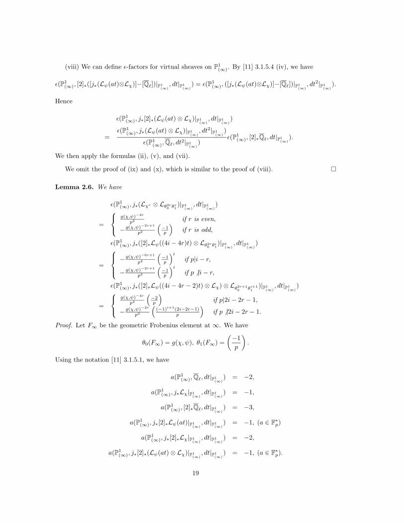
Lemma 2.6. We have
ǫ(P1(∞), j∗(Lχr ⊗ Lθ2r
0 θr1)|P1
(∞), dt|P1
(∞))
=
g(χ,ψ)−4r
p2 if r is even,
− g(χ,ψ)−2r+1
p2
(
−1p
)
if r is odd,
ǫ(P1(∞), j∗([2]∗Lψ((4i − 4r)t) ⊗ Lθ2r
0 θi1)|P1
(∞), dt|P1
(∞))
=
− g(χ,ψ)−6r+1
p4
(
−1p
)i
if p|i − r,
− g(χ,ψ)−2r+1
p3
(
−1p
)i
if p 6 |i − r,
ǫ(P1(∞), j∗([2]∗Lψ((4i − 4r − 2)t) ⊗ Lχ) ⊗ Lθ2r+1
0 θi+11
)|P1(∞)
, dt|P1(∞)
)
=
g(χ,ψ)−4r
p4
(
−2p
)
if p|2i − 2r − 1,
− g(χ,ψ)−2r
p3
(
(−1)i+1(2i−2r−1)p
)
if p 6 |2i − 2r − 1.
Proof. Let F∞ be the geometric Frobenius element at ∞. We have
θ0(F∞) = g(χ, ψ), θ1(F∞) =
(−1
p
)
.
Using the notation [11] 3.1.5.1, we have
a(P1(∞), Qℓ, dt|P1
(∞)) = −2,
a(P1(∞), j∗Lχ|P1
(∞), dt|P1
(∞)) = −1,
a(P1(∞), [2]∗Qℓ, dt|P1
(∞)) = −3,
a(P1(∞), j∗[2]∗Lψ(at)|P1
(∞), dt|P1
(∞)) = −1, (a ∈ F∗
p)
a(P1(∞), j∗[2]∗Lχ|P1
(∞), dt|P1
(∞)) = −2,
a(P1(∞), j∗[2]∗(Lψ(at) ⊗ Lχ)|P1
(∞), dt|P1
(∞)) = −1, (a ∈ F∗
p).
19

So by [11] 3.1.5.6, we have
ǫ(P1(∞), j∗(Lχr ⊗ Lθ2r
0 θr1)|P1
(∞), dt|P1
(∞))
=
{
((θ2r0 θr
1)(F∞))−2ǫ(P1(∞), Qℓ, dt|P1
(∞)) if r is even,
((θ2r0 θr
1)(F∞))−1ǫ(P1(∞), j∗Lχ|P1
(∞), dt|P1
(∞)) if r is odd,
ǫ(P1(∞), j∗([2]∗Lψ((4i − 4r)t) ⊗ Lθ2r
0 θi1)|P1
(∞), dt|P1
(∞))
=
{
((θ2r0 θi
1)(F∞))−3ǫ(P1(∞), [2]∗Qℓ, dt|P1
(∞)) if p|i − r,
((θ2r0 θi
1)(F∞))−1ǫ(P1(∞), j∗[2]∗Lψ((4i − 4r)t)|P1
(∞), dt|P1
(∞)) if p 6 |i − r,
ǫ(P1(∞), j∗([2]∗(Lψ((4i − 4r − 2)t) ⊗ Lχ) ⊗ Lθ2r+1
0 θi+11
)|P1(∞)
, dt|P1(∞)
)
=
{
((θ2r+10 θi+1
1 )(F∞))−2ǫ(P1(∞), j∗[2]∗Lχ|P1
(∞), dt|P1
(∞)) if p|2i − 2r − 1,
((θ2r+10 θi+1
1 )(F∞))−1ǫ(P1(∞), j∗[2]∗(Lψ((4i − 4r − 2)t) ⊗ Lχ)|P1
(∞), dt|P1
(∞)) if p 6 |2i − 2r − 1.
We then apply the formulas in Lemma 2.5.
The following is Proposition 0.4 in the introduction.
Proposition 2.7. ǫ(P1(∞), j∗(Symk(Kl2))|P1
(∞), dt|P1
(∞)) equals
p−(k+1)( k+84 +[ k
2p])
if k = 2r for an even r,
p−(k+1)( k+64 +[ k
2p])
if k = 2r for an odd r, and
(−1)k+12 +[ k
p]−[ k
2p]p−
k+12 ( k+5
2 +[ kp]−[ k
2p])
(−2
p
)[ kp]−[ k
2p]
∏
j∈{0,1,...,[ k2 ]}, p6 |2j+1
(
(−1)j(2j + 1)
p
)
if k = 2r + 1.
Proof. By Lemmas 2.4 and 2.6, ǫ(P1(∞), j∗(Symk(Kl2))|P1
(∞), dt|P1
(∞)) equals
g(χ, ψ)−4r
p2
∏
i∈{0,...,r−1}, p|i−r
(
−g(χ, ψ)−6r+1
p4
(−1
p
)i)
∏
i∈{0,...,r−1}, p6 |i−r
(
−g(χ, ψ)−2r+1
p3
(−1
p
)i)
if k = 2r for an even r,
−g(χ, ψ)−2r+1
p2
(−1
p
)
∏
i∈{0,...,r−1}, p|i−r
(
−g(χ, ψ)−6r+1
p4
(−1
p
)i)
∏
i∈{0,...,r−1}, p6 |i−r
(
−g(χ, ψ)−2r+1
p3
(−1
p
)i)
if k = 2r for an odd r, and
∏
i∈{0,...,r}, p|2i−2r−1
(
g(χ, ψ)−4r
p4
(−2
p
))
∏
i∈{0,...,r}, p6 |2i−2r−1
(
−g(χ, ψ)−2r
p3
(
(−1)i+1(2i − 2r − 1)
p
))
20

if k = 2r + 1. Let’s simplify the above expressions. Recall that g(χ, ψ)2 = p(
−1p
)
. If k = 2r with
r even, we have
ǫ(P1(∞), j∗(Symk(Kl2))|P1
(∞), dt|P1
(∞))
=g(χ, ψ)−4r
p2
∏
i∈{0,...,r−1}, p|i−r
(
−g(χ, ψ)−6r+1
p4
(−1
p
)i)
∏
i∈{0,...,r−1}, p6 |i−r
(
−g(χ, ψ)−2r+1
p3
(−1
p
)i)
=g(χ, ψ)−4r
p2
∏
i∈{0,...,r−1}, p|i−r
g(χ, ψ)−4r
p
∏
i∈{0,...,r−1}
(
−g(χ, ψ)−2r+1
p3
(−1
p
)i)
=g(χ, ψ)−4r
p2
(
g(χ, ψ)−4r
p
)[ rp] (
−g(χ, ψ)−2r+1
p3
)r (−1
p
)
r(r−1)2
=p−2r
p2
(
p−2r
p
)[ rp]
(
p(
−1p
))
r(−2r+1)2
p3r
(−1
p
)
r(r−1)2
= p−r2− 92 r−2−(2r+1)[ r
p]
(−1
p
)− r2
2
= p−(k+1)( k+84 +[ k
2p]).
If k = 2r with r odd, we have
ǫ(P1(∞), j∗(Symk(Kl2))|P1
(∞), dt|P1
(∞))
= −g(χ, ψ)−2r+1
p2
(−1
p
)
∏
i∈{0,...,r−1}, p|i−r
(
−g(χ, ψ)−6r+1
p4
(−1
p
)i)
×∏
i∈{0,...,r−1}, p6 |i−r
(
−g(χ, ψ)−2r+1
p3
(−1
p
)i)
= −g(χ, ψ)−2r+1
p2
(−1
p
)
∏
i∈{0,...,r−1}, p|i−r
(
g(χ, ψ)−4r
p
)
∏
i∈{0,...,r−1}
(
−g(χ, ψ)−2r+1
p3
(−1
p
)i)
= −g(χ, ψ)−2r+1
p2
(−1
p
)(
g(χ, ψ)−4r
p
)[ rp] (
−g(χ, ψ)−2r+1
p3
)r (−1
p
)
r(r−1)2
=g(χ, ψ)(−2r+1)(r+1)
p3r+2
(−1
p
)1+r(r−1)
2(
g(χ, ψ)−4r
p
)[ rp]
=
(
p(
−1p
))
(−2r+1)(r+1)2
p3r+2
(−1
p
)1+r(r−1)
2(
p−2r
p
)[ rp]
= p−r2− 72 r− 3
2−(2r+1)[ rp]
(−1
p
)− (r−1)(r+3)2
= p−(k+1)( k+64 +[ k
2p]).
21

If k = 2r + 1 is odd, we have
ǫ(P1(∞), j∗(Symk(Kl2))|P1
(∞), dt|P1
(∞))
=∏
i∈{0,...,r}, p|2i−2r−1
(
g(χ, ψ)−4r
p4
(−2
p
))
∏
i∈{0,...,r}, p6 |2i−2r−1
(
−g(χ, ψ)−2r
p3
(
(−1)i+1(2i − 2r − 1)
p
))
=
(
−g(χ, ψ)−2r
p3
)r+1 (
−g(χ, ψ)−2r
p
(−2
p
))[ kp]−[ k
2p]
∏
i∈{0,...,r}, p6 |2i−2r−1
(
(−1)i+1(2i − 2r − 1)
p
)
=
(
−p−3−r
(−1
p
)−r)r+1 (
−p−1−r
(−1
p
)−r (−2
p
)
)[ kp]−[ k
2p]
∏
j∈{0,...,r}, p6 |2j+1
(
(−1)r−j(2j + 1)
p
)
= (−1)r+1+[ kp]−[ k
2p]p−(r+1)(r+3+[ k
p]−[ k
2p])
(−2
p
)[ kp]−[ k
2p] (−1
p
)−r(r+1)−r([ kp]−[ k
2p])
×∏
j∈{0,...,r},p6 |2j+1
(
(−1)r−j(2j + 1)
p
)
= (−1)k+12 +[ k
p]−[ k
2p]p−
k+12 ( k+5
2 +[ kp]−[ k
2p])
(−2
p
)[ kp]−[ k
2p]
∏
j∈{0,...,[ k2 ]}, p6 |2j+1
(
(−1)j(2j + 1)
p
)
.
References
[1] M. Artin, A. Grothendieck, and J.-L. Verdier, Theorie des topos et cohomologie etale des
schemas (SGA 4), Lecture Notes in Math. 269, 270, 305, Springer-Verlag (1972-1973).
[2] H.T. Choi and R.J. Evans, Congruences for sums of powers of Kloosterman sums, Inter. J.
Number Theory, 3(2007), 105-117.
[3] P. Deligne, Applications de la Formule des Traces aux Sommes Trigonometriques, in Coho-
mologie Etale (SGA 412 ), 168-232, Lecture Notes in Math. 569, Springer-Verlag 1977.
[4] R. J. Evans, Seventh power moments of Kloosterman sums, Israel J. Math., to appear.
[5] L. Fu, Calculation of ℓ-adic local Fourier transformations, arXiv: 0702436 [math.AG] (2007).
[6] L. Fu and D. Wan, Trivial factors for L-functions of symmetric products of Kloosterman
sheaves, Finite Fields and Appl. 14 (2008), 549-570.
[7] L. Fu and D. Wan, L-functions for symmetric products of Kloosterman sums, J. Reine Angew.
Math. 589 (2005), 79-103.
22

[8] L. Fu and D. Wan, L-functions of symmetric products of the Kloosterman sheaf over Z, Math.
Ann. 342 (2008), 387-404.
[9] K. Hulek, J. Spandaw, B. van Geemen and D. van Straten, The modularity of the Barth-Nieto
quintic and its relative, Adv. Geom., 1(2001), no.3, 263-289.
[10] N. Katz, Gauss sums, Kloosterman sums, and monodromy groups, Princeton University Press
1988.
[11] G. Laumon, Transformation de Fourier, constantes d’equations fontionnelles, et conjecture de
Weil, Publ. Math. IHES 65 (1987), 131-210.
[12] M. Moisio, The moments of Kloosterman sums and the weight distribution of a Zetterberg-
type binary cyclic code, IEEE, Trans. Inform. Theory, 53(2007), 843-847.
[13] M. Moisio, On the moments of Kloosterman sums and fibre products of Kloosterman curves,
Finite Fields Appl., 14(2008), 515-531.
[14] C. Peters, J. Top and M. van der Vlugt, The Hasse zeta function of a K3 surface related to the
number of words of weight 5 in the Melas codes, J. Reine Angew. Math. 432(1992), 151-176.
[15] P. Robba, Symmetric powers of p-adic Bessel functions, J. Reine Angew. Math., 366(1986),
194-220.
[16] J.-P. Serre, Linear representations of finite groups, Springer-Verlag (1977).
[17] J.-P. Serre, Local fields, Springer-Verlag, 1979.
[18] D. Wan, Dwork’s conjecture on unit root zeta functions, Ann. Math., 150(1999), 867-927.
23