Embed Size (px)
Citation preview

FACULTY OF ENGINEERING Departement of Fundamental Electricity and Instrumentation (ELEC) Pleinlaan 2 – 1050 Brussels
Wiener system identification
with generalized orthonormal basis functions
Thesis submitted in fulfilment of the requirements for the degree of Doctor in Engineering (Doctor in de Ingenieurswetenschappen) by
Koen Tiels
March 2015
Advisor: Prof. Dr. ir. Johan Schoukens


FACULTY OF ENGINEERING
Department of Fundamental Electricity and Instrumentation (ELEC)
Pleinlaan 2 – 1050 Brussels
Wiener system identificationwith generalized orthonormal basis functions
Thesis submitted in fulfilment of the requirements for the degree ofDoctor in Engineering (Doctor in de Ingenieurswetenschappen) by
Koen Tiels
Advisor: Prof. Dr. ir. Johan Schoukens
Members of the jury: Prof. Dr. ir. Fouad GiriUniversite de Caen Basse-Normandie, France
Dr. Peter S. C. HeubergerTechnische Universiteit Eindhoven, Nederland
Dr. Anna MarconatoVrije Universiteit Brussel
Prof. Dr. Steve Vanlanduit (President)Universiteit Antwerpen, Belgie
Prof. Dr. ir. Johan Deconinck (Vice-President)Vrije Universiteit Brussel
Prof. Dr. ir. Gerd Vandersteen (Secretary)Vrije Universiteit Brussel

Copyright, ISBN, etc. to be added later.

Acknowledgments
The big moment is almost there! After four and a half years of research andpreparing the manuscript I am ready to defend my thesis. But, a PhD thesisis not the work of one person alone. It involves interactions with many people:discussions, reading about the work of others, presenting own work and receivingconstructive feedback, etc. Therefore, I would like to thank everyone that inone way or another contributed to the completion of this thesis. There are,however, some persons I like to thank explicitly.
First of all, I thank Johan Schoukens, my advisor, for giving me the oppor-tunity to pursue a PhD at the ELEC department, for being an inexhaustiblesource of good ideas, for the inspiring discussions, for proofreading my papersand thesis, and for many more things. Johan, without you, I wouldn’t havebeen able to complete this thesis.
I also thank the jury members for their careful reading of the thesis and fortheir feedback that helped me improve the manuscript.
In the first year of my PhD, I had the opportunity to visit the Delft Centerfor Systems and Control. This visit was really helpful to me and I learned a lotduring that one month. Thank you Paul (Van den Hof), Peter (Heuberger) andRoland (Toth) for your hospitality and for the nice discussions on orthonormalbasis functions and their application in block-oriented modeling.
In the last year of my PhD, I had the opportunity to visit INRIA Rennes forone month. Thank you Qinghua (Zhang) for your hospitality. The visit helpedme sharpen my mind.
I thank Maarten Schoukens for carrying out the measurements on the log-arithmic amplifier and on the two-branch Wiener-Hammerstein system. I alsothank Anna, Maarten, Dhammika, and Amjad for the collaboration on insulin-glucose models. I thank Johan, Rik, Yves, Gerd, Maarten, Anne, Laurent,and David (Westwick) for discussions on block-oriented modeling, and Johan,Mariya, Philippe, Gabriel, Maarten, Konstantin, Anne, Laurent, Ivan, andLieven (De Lathauwer) for discussions on tensors and their decompositions.
Ik dank Ann, Jenny, Bea en Annick voor de administratieve ondersteuningen Sven, Johan, Lut en Wim voor de technische ondersteuning. Dankzij jullie

hulp kon ik mij voornamelijk toeleggen op de wetenschappelijke en educatieveaspecten van het doctoraat.
I thank the (former and current) colleagues and the visitors at the ELECdepartment, be it for supervising together the labs of electricity or the exercisesessions during the Spring School, for giving or pointing me to inspiring talks,for organizing an international cooking dinner, for organizing sports events, forthe trips to Christmas markets and to the Belgian coast, for making me feellike a schtroumpf, for the visit to Hungary and the road trip back to Brussels,or just for a drink and a chat. The warm and inspiring atmosphere at thedepartment contributed to a pleasant and (hopefully) successful completion ofmy PhD research.
Tenslotte dank ik mijn ouders, mijn broer en alle andere familieleden vooralle steun en aanmoedigingen. Bart, bedankt voor al je goede raad. Je outside-of-the-box denken heeft me veel geholpen. Mama en papa, bedankt voor julliesteun en vertrouwen waarop ik telkens kon rekenen.
Koen Tiels
BrusselsMarch 2015
6

Contents
Notation vSymbols . . . . . . . . . . . . . . . . . . . . . . . . . . . . . . . . . . . vAcronyms . . . . . . . . . . . . . . . . . . . . . . . . . . . . . . . . . . xiNotational conventions and operators . . . . . . . . . . . . . . . . . . xii
1 Introduction 11.1 Context . . . . . . . . . . . . . . . . . . . . . . . . . . . . . . . . 1
1.1.1 System identification . . . . . . . . . . . . . . . . . . . . . 11.1.2 Model structures . . . . . . . . . . . . . . . . . . . . . . . 31.1.3 Block-oriented models . . . . . . . . . . . . . . . . . . . . 51.1.4 Wiener-Schetzen model . . . . . . . . . . . . . . . . . . . 6
1.2 Questions . . . . . . . . . . . . . . . . . . . . . . . . . . . . . . . 71.3 Overview and outline . . . . . . . . . . . . . . . . . . . . . . . . . 81.4 Publications . . . . . . . . . . . . . . . . . . . . . . . . . . . . . . 9
2 Preliminaries 152.1 Considered signals . . . . . . . . . . . . . . . . . . . . . . . . . . 15
2.1.1 Gaussian noise and multisines . . . . . . . . . . . . . . . . 152.1.2 Equivalence between both . . . . . . . . . . . . . . . . . . 16
2.2 Considered systems . . . . . . . . . . . . . . . . . . . . . . . . . . 172.2.1 Uniform versus mean-square convergence . . . . . . . . . 172.2.2 Volterra series . . . . . . . . . . . . . . . . . . . . . . . . 182.2.3 The class of Wiener systems . . . . . . . . . . . . . . . . . 192.2.4 Universal approximation . . . . . . . . . . . . . . . . . . . 21
2.3 The best linear approximation . . . . . . . . . . . . . . . . . . . 212.3.1 Definition . . . . . . . . . . . . . . . . . . . . . . . . . . . 212.3.2 Existence and invariance . . . . . . . . . . . . . . . . . . . 222.3.3 Initialization of dynamics in block-oriented models . . . . 23
2.4 Orthonormal basis functions . . . . . . . . . . . . . . . . . . . . . 242.4.1 Finite impulse response model . . . . . . . . . . . . . . . 24
i

CONTENTS
2.4.2 Infinite impulse response models . . . . . . . . . . . . . . 25
2.4.3 Rational orthonormal basis functions . . . . . . . . . . . . 26
2.4.4 Pole locations and OBF structures . . . . . . . . . . . . . 27
2.4.5 Error bound . . . . . . . . . . . . . . . . . . . . . . . . . . 27
2.5 Conclusion . . . . . . . . . . . . . . . . . . . . . . . . . . . . . . 28
2.A BLA of a polynomial Wiener-Hammerstein system . . . . . . . . 30
2.B Intermezzo: (non-)orthogonal polynomials . . . . . . . . . . . . . 31
2.C Extra basis function . . . . . . . . . . . . . . . . . . . . . . . . . 31
3 Making Wiener-Schetzen less parameter expensive 35
3.1 Wiener system identification . . . . . . . . . . . . . . . . . . . . . 35
3.2 Setup . . . . . . . . . . . . . . . . . . . . . . . . . . . . . . . . . 36
3.2.1 System . . . . . . . . . . . . . . . . . . . . . . . . . . . . 36
3.2.2 Signals . . . . . . . . . . . . . . . . . . . . . . . . . . . . . 37
3.2.3 Model . . . . . . . . . . . . . . . . . . . . . . . . . . . . . 38
3.3 OBFs based on the poles of the BLA . . . . . . . . . . . . . . . . 38
3.3.1 Basic idea . . . . . . . . . . . . . . . . . . . . . . . . . . . 39
3.3.2 Identification procedure (no output noise) . . . . . . . . . 39
3.3.3 Noise analysis . . . . . . . . . . . . . . . . . . . . . . . . . 42
3.3.4 Illustration . . . . . . . . . . . . . . . . . . . . . . . . . . 42
3.3.5 Conclusion . . . . . . . . . . . . . . . . . . . . . . . . . . 46
3.4 The BLA as a basis function . . . . . . . . . . . . . . . . . . . . 46
3.4.1 Basic idea . . . . . . . . . . . . . . . . . . . . . . . . . . . 47
3.4.2 Parameter reduction step . . . . . . . . . . . . . . . . . . 47
3.4.3 Extension to MISO single-branch Wiener systems . . . . . 49
3.4.4 Illustration . . . . . . . . . . . . . . . . . . . . . . . . . . 53
3.4.5 Conclusion . . . . . . . . . . . . . . . . . . . . . . . . . . 58
3.5 Iterative update of the pole locations . . . . . . . . . . . . . . . . 59
3.5.1 Basic idea . . . . . . . . . . . . . . . . . . . . . . . . . . . 61
3.5.2 Causes for pole mismatch . . . . . . . . . . . . . . . . . . 61
3.5.3 Iterative update scheme . . . . . . . . . . . . . . . . . . . 63
3.5.4 Illustration . . . . . . . . . . . . . . . . . . . . . . . . . . 65
3.5.5 Conclusion . . . . . . . . . . . . . . . . . . . . . . . . . . 68
3.6 Overall conclusion . . . . . . . . . . . . . . . . . . . . . . . . . . 70
3.A Normalized Q-polynomials . . . . . . . . . . . . . . . . . . . . . . 71
3.B Proof of Lemma 3.9 . . . . . . . . . . . . . . . . . . . . . . . . . 71
3.C Proof of Lemma 3.10 . . . . . . . . . . . . . . . . . . . . . . . . . 72
3.D Proof of Theorem 3.11 . . . . . . . . . . . . . . . . . . . . . . . . 73
3.E Influence of output noise . . . . . . . . . . . . . . . . . . . . . . . 74
3.F Reduced number of parameters in the MISO case . . . . . . . . . 74
ii

CONTENTS
4 Usefulness universal approximation property in practice 754.1 A Wiener-like system . . . . . . . . . . . . . . . . . . . . . . . . . 75
4.1.1 Description of the circuit . . . . . . . . . . . . . . . . . . 754.1.2 The measurement data . . . . . . . . . . . . . . . . . . . . 764.1.3 Estimation of Wiener-Schetzen models . . . . . . . . . . . 764.1.4 The parameter reduction step . . . . . . . . . . . . . . . . 794.1.5 Conclusion . . . . . . . . . . . . . . . . . . . . . . . . . . 79
4.2 A discrete-time Hammerstein system . . . . . . . . . . . . . . . . 804.2.1 Description of the system . . . . . . . . . . . . . . . . . . 804.2.2 The simulation data . . . . . . . . . . . . . . . . . . . . . 804.2.3 A Volterra series approximation . . . . . . . . . . . . . . . 814.2.4 A Wiener-Schetzen model approximation . . . . . . . . . 814.2.5 Conclusion . . . . . . . . . . . . . . . . . . . . . . . . . . 82
4.3 A nonlinear feedback system: the Silverbox . . . . . . . . . . . . 834.3.1 Description of the device . . . . . . . . . . . . . . . . . . . 834.3.2 The measurement data . . . . . . . . . . . . . . . . . . . . 844.3.3 Direct estimation of a Wiener-Schetzen model . . . . . . . 854.3.4 Unfolding the feedback loop . . . . . . . . . . . . . . . . . 864.3.5 Conclusion . . . . . . . . . . . . . . . . . . . . . . . . . . 88
4.4 Overall conclusion . . . . . . . . . . . . . . . . . . . . . . . . . . 894.A Truncation error of the Hammerstein system . . . . . . . . . . . 904.B Volterra series approximation of the Silverbox . . . . . . . . . . . 91
5 Dynamics at the output: Wiener-Hammerstein models 935.1 Wiener-Hammerstein system identification . . . . . . . . . . . . . 93
5.1.1 Applications . . . . . . . . . . . . . . . . . . . . . . . . . 935.1.2 Identification methods . . . . . . . . . . . . . . . . . . . . 945.1.3 Initial estimates . . . . . . . . . . . . . . . . . . . . . . . 945.1.4 Initialization methods that start from the BLA . . . . . . 945.1.5 Parallel Wiener-Hammerstein systems . . . . . . . . . . . 96
5.2 Initial estimates using basis function expansions . . . . . . . . . . 965.2.1 Setup . . . . . . . . . . . . . . . . . . . . . . . . . . . . . 965.2.2 Basic idea . . . . . . . . . . . . . . . . . . . . . . . . . . . 975.2.3 Proposed method . . . . . . . . . . . . . . . . . . . . . . . 985.2.4 Illustration . . . . . . . . . . . . . . . . . . . . . . . . . . 1025.2.5 Conclusion . . . . . . . . . . . . . . . . . . . . . . . . . . 104
5.3 Initial estimates using phase-coupled multisines . . . . . . . . . . 1075.3.1 Setup . . . . . . . . . . . . . . . . . . . . . . . . . . . . . 1075.3.2 Basic idea . . . . . . . . . . . . . . . . . . . . . . . . . . . 1085.3.3 Phase-coupled multisine excitation . . . . . . . . . . . . . 1085.3.4 New terms in the output spectrum of the BLA . . . . . . 1095.3.5 The shifted BLA and parametric smoothing . . . . . . . . 112
iii

CONTENTS
5.3.6 Generalization to arbitrary degree polynomial nonlinearities1145.3.7 Illustration . . . . . . . . . . . . . . . . . . . . . . . . . . 1155.3.8 Conclusion . . . . . . . . . . . . . . . . . . . . . . . . . . 121
5.4 From coupled to decoupled polynomial representations . . . . . . 1215.4.1 Setup . . . . . . . . . . . . . . . . . . . . . . . . . . . . . 1215.4.2 Basic idea . . . . . . . . . . . . . . . . . . . . . . . . . . . 1235.4.3 Simultaneous decoupling of quadratic polynomials . . . . 1235.4.4 Simultaneous decoupling of cubic polynomials . . . . . . . 1265.4.5 Simultaneous decoupling of polynomials with mixed de-
grees of nonlinearity . . . . . . . . . . . . . . . . . . . . . 1285.4.6 Illustration . . . . . . . . . . . . . . . . . . . . . . . . . . 1295.4.7 Conclusion . . . . . . . . . . . . . . . . . . . . . . . . . . 132
5.5 Overall conclusion . . . . . . . . . . . . . . . . . . . . . . . . . . 1325.A Time origin . . . . . . . . . . . . . . . . . . . . . . . . . . . . . . 1345.B Dominant terms in the shifted BLA . . . . . . . . . . . . . . . . 134
6 Conclusions 1376.1 Conclusions . . . . . . . . . . . . . . . . . . . . . . . . . . . . . . 1376.2 Contributions . . . . . . . . . . . . . . . . . . . . . . . . . . . . . 1396.3 Future work . . . . . . . . . . . . . . . . . . . . . . . . . . . . . . 140
Publication list 143
Bibliography 147
iv

Notation
Symbols
Symbol Description
ai Denominator coefficients of a transfer functionaNL Nonlinear stiffness coefficient (in N m−3)A(q) Denominator polynomial of a transfer functionbi Numerator coefficients of a transfer functionB(q) Numerator polynomial of a transfer function
B[i] Symmetric matrix of quadratic polynomial coefficients
β[i]i1,i2
B[i] Symmetric tensor of cubic polynomial coefficients
β[i]i1,i2,i3
c0, cs, c−s (Complex) constant gainsc1, c2 Arbitrary constantscBLA Constant gainceq, ceq1
, ceq1Arbitrary non-zero constants
cGOBF Constantci Coefficients of a linear combination of OBFscshift Constant positive integerC Set of complex numbers
C1 Upper bound of∑∞d=1 CKdCU
d
C2 Upper bound of ρCKd Upper bound of |Kd|CU Upper bound of
√2U( ω2π )
d Degree of nonlinearityD Maximum degree of nonlinearitye Error signal
Continued on next page
v

NOTATION
Continued from previous pageE E := z ∈ C : |z| > 1 is the exterior of the unit disk
including infinityf(u) Static nonlinear function f operating on uf(u1, . . . , un) Multivariate static nonlinear function f operating on
u1, . . . , unfs Sample frequency (in Hz)F Matrix containing the spectra of a set of GOBFsFi(q) Orthonormal basis functionFi(z) Z-transform of the impulse response fi(τ)g(τ) Impulse response of linear dynamic system GG(q) Discrete-time linear dynamic systemGBLA Frequency response function of the best linear approx-
imationGM Parametric transfer function modelG+
SBLA, G−SBLA Frequency response function of the shifted best linear
approximations that are proportional to S(k)R(k + s)and S(k)R(k − s), respectively
H2(E) Hardy space of functions that are squared integrableon T and analytic on E
Hd(u(t)) dth-degree normalized Hermite polynomialHd[x(t)] dth-order Volterra operator in the Silverbox examplei Indeximax Positive integer that determines the bandwidth of a
phase-coupled multisinej j2 = −1J Regression matrixk Frequency bink Indexk1(τ) Impulse response of a linear dynamic systemkd(τ1, . . . , τd) dth-order Volterra kernel
kωi kωi =⌊ωiN2πfs
⌋
K(s) Second-order system in the Silverbox exampleK(θ) Cost function in θKdu1, . . . , ud dth-order Volterra operator; Kdu, . . . , u = Kd[u]Kd(Lk, l1, l2, . . . , ld−1) Symmetrized frequency domain representation of
kd(τ1, . . . , τd)KN Cost function that depends upon the number of sam-
ples NK(p) pth-order inverse of a Volterra operatorl Index, mostly over the frequency bins
Continued on next page
vi

NOTATION
Continued from previous pageli Index over the frequency bins
Lk Frequency bin such that k = Lk +∑d−1i=0 li
M Number of branches in a parallel Wiener-Hammersteinmodel belonging to the class SM
Mcubic Partially symmetric tensor in which each of the tensorsB[i] is stacked
Mmixed Partially symmetric tensor in which the matrices B[i]
and the tensors B[i] are stored
Mquad Partially symmetric tensor in which each of the ma-trices B[i] is stacked
n Number of FIR coefficients/OBFs, possibly aug-mented with one or more feed-through terms
n Number of branches in a parallel Wiener-Hammersteinmodel
n1 Number used in determining the rank of a regressionmatrix J
na Degree of the denominator polynomial in a transferfunction
nb Degree of the numerator polynomial in a transfer func-tion
nblocks Number of experiment blocksncubic Number of branches in a parallel Wiener-Hammerstein
model with only cubic nonlinearitiesnexp Number of experimentsni Number of OBFs in the ith set of OBFs, possibly aug-
mented with a feed-through termnmixed Number of branches in a parallel Wiener-Hammerstein
model with only quadratic and cubic nonlinearitiesnp Number of poles of a linear dynamic systemnquad Number of branches in a parallel Wiener-Hammerstein
model with only quadratic nonlinearitiesnrep Number of pole repetitionsnu Number of inputsnα Number of GOBFsnβ Number of polynomial coefficientsnξ Number of pole estimatesN Number of samples (per period)O(·) Big-O notation, indicates boundedness of a determin-
istic sequence (see further)Op(·) Indicates boundedness in probability (see further)
Continued on next page
vii

NOTATION
Continued from previous pagep Real pole of a first-order systemp Order of a pth-order inverse K(p)
pi Pole location of a linear dynamic systemP Number of periodsP (·) Probability ofq Forward shift operator (qu(t) = u(t+ 1))q−1 Backward shift operator (q−1u(t) = u(t− 1))Q[x(t)] Volterra operator in the Silverbox example
Q(d)i1i2...id
(x) Multivariate (normalized) Hermite polynomial, calledQ-polynomial
R(q) Wiener dynamicsR Set of real numbersR+ Set of positive real numberss Positive integer that determines the frequency offset
of the input dynamics in the shifted BLAS(q) Hammerstein dynamics
Sdl Sdl := sk : sk ∈ −s, 0, s ∧∑dk=1 sk = l
SM Subclass of parallel Wiener-Hammerstein modelsSUU (Auto-)power spectrum of u(t) (SUU (k) =
Eu|U(k)|2)SY U Cross-power spectrum of y(t) and u(t) (SY U (k) =
EuY (k)U∗(k))t Discrete time (in number of samples)t Continuous time (in s) (t = t/fs at the sampling in-
stants)T Maximal number of delays considered in a Volterra
series expansion (as a number of samples)T T := z ∈ C : |z| = 1 is the unit circleu Input signalU( ω2π ) Uniformly bounded function in the definition of a mul-
tisineUk Fourier coefficientv Output noisew Intermediate signalW Matrix containing the spectra of the intermediate sig-
nals wi(t)W (k) Weighting sequence in the frequency domainx Intermediate signalx⊥BLA Output of an OBF that is proportional to the para-
metric estimate of the BLAContinued on next page
viii

NOTATION
Continued from previous pagey Output signaly Displacement (in m) in the Silverbox exampley Velocity (in m s−1) in the Silverbox exampley Acceleration (in m s−2) in the Silverbox exampley0 Noise-free output signalyDC Estimate of the DC component at the outputyS Stochastic nonlinear noise sourceyβ Output of a multivariate polynomial with coefficients
βY(k) Collection of DFT spectra of several output signals in
a vectorYd Output spectrum of a Wiener-Hammerstein model
with a pure dth-degree nonlinearityz Variable of the Z-transform
α Coefficients of a linear combination of GOBFsβ Collection of multivariate polynomial coefficientsβr Collection of multivariate polynomial coefficients of a
polynomial with a reduced number of parametersγd Polynomial coefficient corresponding to a dth-degree
monomialδij Kronecker delta (δii = 1, δij = 0 if i 6= j)
δ Time shift∆pi Difference between the estimated and the true pole pi,
i.e. ∆pi = pi − pi∆x Difference between the true intermediate signal x(t)
and its approximation∆φ Phase shift due to a shifted time originε (Typically small) positive numberζ Positive integer that determines the frequency resolu-
tion of a phase-coupled multisine
η[i]k Scalar coefficient in the canonical polyadic decompo-
sition of B[i]
θ Model parametersκi Coefficients of a linear combination of matricesλk Basis vector in the canonical polyadic decomposition
of B[i]
µ[i]k Scalar coefficient in the canonical polyadic decompo-
sition of B[i]
ν The excited frequencies in a phase-coupled multisineare at frequencies ν and ν + s
Continued on next page
ix

NOTATION
Continued from previous pageξ Pole estimate, pole locationρ Measure for how close the estimated poles are to the
true polesσ2u Variance of the signal u(t)τ Discrete time (in number of samples)τ Continuous time (in s)Υd Ratio of the contributions in Yd in which the input
dynamics shift over s and those in which the inputdynamics shift over 2s
φ Phase shift of the poles and the zeros of the inputdynamics with respect to their complex conjugates
φk Phase of the DFT coefficient at the kth frequency binψk Basis vector in the canonical polyadic decomposition
of B[i]
ω Angular frequency (in rad s−1)ωp Normalized passband edge frequency of a Chebyshev
filter
The notations O(·), and Op(·) are explained in more detail hereafter.
Notation 0.1 (O(·)). The notation h1 is an O(Nn) indicates that for N bigenough, |h1(N)| ≤ cNn, where c is a strictly positive real number.
Notation 0.2 (Op(·), [van der Vaart, 1998]). The notation h2 is an Op(Nn)
indicates that the sequence h2(N) is bounded in probability at the rate Nn.More precisely, h2(N) = h3(N)Nn, where h3(N) is a sequence that is boundedin probability.
x

NOTATION
Acronyms
Acronym Description
AIC Akaike’s information criterionALS Alternating least-squaresBLA Best linear approximationCANDECOMP Canonical decompositionCPD Canonical polyadic decompositionDC Direct current, but mostly used here to indicate the mean
value (contribution at zero frequency) of a signalDFT Discrete Fourier transformDVD Digital versatile discFIR Finite impulse responseFRF Frequency response functionGOBF Generalized orthonormal basis functionIFAC International Federation of Automatic Controli.i.d. Independent and identically distributedIIR Infinite impulse responseINDSCAL Individual differences in scalingLS Least squaresLTI Linear and time-invariantMDL Minimum description lengthMIMO Multiple input multiple outputMISO Multiple input single outputMLE Maximum likelihood estimatorMSE Mean-square errorNARMAX Nonlinear autoregressive moving average model with exoge-
nous inputsOBF Orthonormal basis functionPARAFAC Parallel factorsPEM Prediction error methodPISPO Period in same period outPNLSS Polynomial nonlinear state-spaceQBLA Quadratic best linear approximationrms Root mean squareSISO Single input single outputSNR Signal-to-noise ratioSVD Singular value decompositionSVM Support vector machineTISO Two input single outputWS Wiener-Schetzen
xi

NOTATION
Notational conventions and operators
Notation Description
Bold symbols Vectors or matrices, e.g. α, JBold calligraphic symbols Tensors, e.g. Mx(t), X(k) Signal and its DFT spectrumG(q), g(τ) Discrete-time LTI system and its impulse responseG(z) Z-transform of g(τ)
(·) Estimate, e.g. y is an estimate of y˙(·) Time derivative, e.g. y = dy
dt
(·) Second time derivative, e.g. y = d2ydt2
(·) Subtracts the DC value of a signal, e.g.y = y − Ey
(·) Explicitly indicates a coupled representation of a
nonlinear function (e.g. with cross-terms if thefunction is a polynomial), or a signal or LTI system
associated with the function, e.g.f ,x(t),
R(q)
(·) Originates from true model parameters, e.g. θ arethe true model parameters
(·)[i] ith element in a sequence(·)T Matrix transpose(·)∗ Complex conjugation(·)⊥ Explicitly indicates orthogonality(·) 6⊥ Explicitly indicates lack of orthogonality(·)! Factorial, e.g. d! = d(d− 1) · · · 1(n+DD
)Binomial coefficient, indicates the number of com-binations of D elements that can be made out of aset of n+D elements,
(n+DD
)= (n+D)!
n!D!b·c Floor function, i.e. bxc is the largest integer not
greater than x〈·, ·〉 Inner product, e.g. 〈F1, F2〉 is the in-
ner product between two transfer functionsF1(z), F2(z) ∈ H2(E)
∠U(k) Phase of a complex number U(k)|U(k)| Amplitude of a complex number U(k)‖·‖2 Two-norm‖·‖∞ Infinity norm‖·‖F Frobenius norm∝ Is proportional to
Continued on next page
xii

NOTATION
Continued from previous page:= Is defined as
∗ Convolution, e.g. g(t)∗u(t) =∫ +∞−∞ g(τ)u(t− τ)dτ
Tensor product⊗ Kronecker productKdu1, . . . , ud dth-order Volterra operator; Kdu, . . . , u = Kd[u]L· Laplace transformL−1· Inverse Laplace transformE· Expected valueEu· Ensemble average over an input classE· Generalized expected value
Ex(t) := limN→∞
1NEx(t)
arg minθK(θ) Minimizing argument of K(θ)atan(·) Inverse of the tangent functioncorank(·) Corank of a matrix, i.e. the dimensionality of its
null spacemin(·) Minimummax(·) Maximumperm(l1, l2, l3) All possible permutations of (l1, l2, l3)plim Limit in probability (see further)vec(·) Vectorization of a matrix, stacks the columns of
the matrix on top of each other
The notation plim is explained in more detail hereafter.
Notation 0.3 (plim, [Pintelon and Schoukens, 2012]). The sequence h(N), forN = 1, 2, . . . converges to h in probability if, for every ε, δ > 0 there exists anN0 such that for every N > N0 : P (|h(N)− h| ≤ ε) > 1− δ. We write
plimN→∞
h(N) = h⇔ ∀ε > 0 : limN→∞
P (|h(N)− h| ≤ ε) = 1 .
Remark 0.4. We will often—by abuse of notation—use u(t) to denote thesignal u instead of the instantaneous value.
xiii


Chapter 1
Introduction
This chapter introduces the context of this thesis and presents the main ques-tions that are addressed. It also gives an overview of the content in the remain-ing chapters, and makes the connection with the publications that resulted fromthis thesis.
1.1 Context
This thesis is situated in the context of nonlinear system identification. Here-after, we give a very brief introduction to this subject. More comprehensiveinformation on system identification can be found in e.g. Soderstrom and Sto-ica [1989]; Ljung [1999] and Pintelon and Schoukens [2012].
1.1.1 System identification
A system can be thought of as a device that maps an excitation (an input) toa response (an output). Think for example about a spring scale that fishermenuse to weigh the fish they catch. The input is the fish’s gravitational force thatis applied to the spring. The output is the displacement of the spring. Anotherexample is a loudspeaker, which maps the waveform provided by e.g. a DVDplayer to a sound.
System identification is the process of creating mathematical models of sys-tems from measured input/output data. This is useful, since knowing how theinput is mapped to the output makes it possible to understand the behaviorof the system, to simulate and predict the responses of the system to differentexcitations, and to modify the behavior of the system using a controller. Forexample, if it is known that a loudspeaker attenuates the bass (low frequencies)
1

Chapter 1: Introduction
system
model
+u y
y
e+
−
class ofexcitation
modelclass
errorcriterion
Figure 1.1: When approximating the input/output behavior of a system using a model,three important choices need to be made: the excitation signal, the model class, andthe error criterion.
and amplifies the treble (high frequencies) too much, then the overall behav-ior of the loudspeaker can be improved by first amplifying the low frequenciesand attenuating the high frequencies in the waveform, and next applying thisprefiltered waveform to the loudspeaker.
In system identification, mathematical models of systems are built in a sys-tematical way. The four main steps that need to be performed when buildingthe model are:
1. Excite the system and collect the input/output data.
2. Select an appropriate model structure or model class.
3. Estimate the model parameters.
4. Validate the model on new input/output data.
In these four steps, three important choices need to be made: the class ofexcitation signals, the model class, and the error criterion (see Figure 1.1).
In the first step, a well-designed excitation u is applied to the system, andthe excitation u and the system response y are measured. The excitation shouldbe persistently exciting such that enough information can be collected from themeasured input/output data. For example, the loudspeaker should be excitedby a signal with a sufficiently large bandwidth, such that information aboutboth the low and high frequencies is present in the collected data.
In the second step, an appropriate model class is selected. The model classis a collection of models that have the same structure, e.g. all polynomials ofdegree at most three, all second-order linear state-space models, etc. Manydifferent model structures are available, and choosing an appropriate one is notalways simple. A more detailed explanation of the model selection is given inthe next subsection.
2

1.1 Context
In the third step, the model parameters are estimated. The model structureis typically parameterized in terms of a finite number of parameters, e.g. thepolynomial coefficients, the matrix entries of the state-space model, etc. Thesemodel parameters need to be tuned, such that the model explains the collecteddata as well as possible. This is usually done by minimizing a certain errorcriterion (a distance between the model and the data). A typical choice isto minimize the mean-square distance between the measured and the modeledoutput data, i.e. minimize
1
N
N−1∑
t=0
e2(t) , with e(t) = y(t)− y(θ, t) , (1.1)
with respect to the model parameters θ. This minimization is straightforward ifthe model is linear-in-the-parameters, since then a closed-form solution exists. Ifthe model is nonlinear in its parameters, then typically a nonlinear optimizationneeds to be done, which requires good initial estimates of the model parameters.
In the fourth step, it is checked whether the obtained model can satisfac-torily model new input/output data that were not used to estimate the modelparameters.
1.1.2 Model structures
A crucial step in system identification is choosing an appropriate model class.On the one hand, the model structure should be flexible enough to make itpossible to well approximate the behavior of a large variety of systems. Onthe other hand, the model should be parameter-parsimonious, as the variabilityof the identified model parameters increases with the number of independentparameters [Soderstrom and Stoica, 1989] when the model is identified fromnoisy measurements. A trade-off thus needs to be made between model errors(bias) and noise sensitivity (variance). This trade-off is the well-known bias-variance trade-off.
Depending on the amount of physical knowledge that is used when building amodel, the model is either called a white-box, a gray-box, or a black-box model.White-box modeling only uses first principles or physical laws, e.g. Hooke’s lawin the case of the spring scale, which states that the displacement of the springis proportional to the force applied to it. Depending on the complexity of thesystem, building a white-box model can take quite some effort. Moreover, thebuilding process needs to be done over again for every new system. Black-box modeling uses no physical knowledge about the system, but only uses themeasured input/output data to determine the mapping. Typically, black-boxmodels are flexible mathematical expressions that can well approximate a largevariety of system behaviors. They are thus quite generally applicable, but often
3

Chapter 1: Introduction
use a large number of parameters in return. In between white-box and black-box modeling are different shades of gray-box modeling (see e.g. Ljung [2010]for a classification), where both physical laws and measurements are used. Thisthesis primarily concerns black-box modeling.
In order not to use too many parameters, the model structure should reflectthe properties of the system that is to be modeled. A linear time-invariant(LTI) model is commonly used to approximate the behavior of a dynamicalsystem (a system with memory). A system is linear if its steady-state behaviorfulfills the superposition principle. This means that if the steady-state responseto an input u1 is y1, and the steady-state response to an input u2 is y2, thenthe steady-state response of a linear system to a linear combination of thoseinputs u = c1u1 + c2u2 is the linear combination of the corresponding steady-state outputs y = c1y1 + c2y2, where c1 and c2 are arbitrary constants. Systemsthat do not fulfill the superposition principle are called nonlinear systems. Asystem is time-invariant if its dynamic behavior does not change with time.This means that if the system responds with an output y(t) to an input u(t),it responds with an output y(t− δ) to a time-shifted input u(t− δ) for everyarbitrary time-shift δ. LTI models are often used, because many systems canbe assumed linear when working with small amplitude ranges of the excitation,and many systems can be assumed time-invariant when working on sufficientlysmall timescales with respect to the time variations. Moreover, LTI models givemuch insight about the behavior of the system, there are many tools availableto estimate LTI models, and the linear identification theory is mature. Never-theless, all physical systems are nonlinear and/or time-varying to some extent,even the spring scale that ideally obeys Hooke’s law. If the fish is too heavy,the spring cannot stretch any further, and hence does not behave linearly any-more. Moreover, the spring constant, i.e. the proportionality constant, changesover time due to wearing. In this thesis, nonlinear time-invariant models areconsidered.
The class of nonlinear systems is extremely large (all systems that are notlinear are nonlinear), hence many different nonlinear model structures havealready been proposed. Examples are nonlinear state-space models [Verdult,2002], the NARMAX model [Chen and Billings, 1989], block-oriented models[Giri and Bai, 2010], Volterra series [Schetzen, 2006], neural networks [Nelles,2001], etc. They all have their advantages and disadvantages. Nonlinear state-space and NARMAX models are quite flexible for example, but provide littleor no physical insight. Block-oriented models are parameter-parsimonious andprovide some physical insight, but the estimation of the more complex block-oriented models often involves nonlinear optimization, and thus requires goodinitial estimates. More information on nonlinear modeling can be found in e.g.Billings [1980]; Sjoberg et al. [1995].
4

1.1 Context
1.1.3 Block-oriented models
This thesis makes extensive use of block-oriented models [Billings and Fakhouri,1982; Giri and Bai, 2010]. These models combine linear dynamic and nonlinearstatic (memoryless) blocks. Due to this highly structured nature, block-orientedmodels offer insight about the system to the user.
In this thesis, we will work with discrete-time linear dynamic blocks, al-though it is possible to handle continuous-time dynamics as well. Note thatblock-oriented models allow for an easy discretization, due to the separationbetween the dynamics and the nonlinearities.
The simplest block-oriented models are the Wiener model (nonlinear staticblock preceded by a linear dynamic block, see Figure 1.2a) and the Hammer-stein model (nonlinear static block followed by a linear dynamic block, seeFigure 1.2b).
A possible generalization is to put more blocks in series, resulting in e.g. aWiener-Hammerstein model (nonlinear static block sandwiched between two lin-ear dynamic blocks, see Figure 1.2c) and a Hammerstein-Wiener model (lineardynamic block sandwiched between two nonlinear static blocks, see Figure 1.2d).
Another possible generalization is to have parallel branches, each contain-ing a single-branch block-oriented model, resulting in e.g. a parallel Wiener-Hammerstein model (see Figure 1.3a). Moreover, the intermediate blocks canhave multiple inputs and/or multiple outputs, resulting in e.g. a parallel Wienermodel with a multivariate nonlinearity (see Figure 1.3b).
Parallel Wiener and parallel Wiener-Hammerstein models are known to beuniversal approximators [Palm, 1979; Boyd and Chua, 1985; Schetzen, 2006].This means that they can approximate the behavior of systems belonging to theclass of Wiener systems arbitrarily well in mean-square sense, i.e. the mean-square error in (1.1) can be made arbitrarily small for these systems. Theclass of Wiener systems should not be confused with the cascade of a lineardynamic and a nonlinear static block (see Figure 1.2a), which is also called aWiener system. Instead, systems belonging to the class of Wiener systems areroughly all time-invariant, non-explosive systems (meaning that their outputhas finite variance for a Gaussian noise excitation), where the influence of theinput infinitely far back in time on the present output decays to zero [Schetzen,2006]. A subset of these systems are the fading memory systems consideredin Boyd and Chua [1985]. In a proper setting, to be specified later, Wienersystems can also deal with discontinuous nonlinearities. A clear advantage ofmodel structures with the universal approximation property is that they arequite flexible. In Chapter 2, we go more into detail on the class of Wienersystems and on the approximation properties of parallel Wiener and parallelWiener-Hammerstein models.
5

Chapter 1: Introduction
G(q) f(x)u(t) x(t) y(t)
(a) Wiener model
f(u) G(q)u(t) w(t) y(t)
(b) Hammerstein model
G1(q) f(x) G2(q)u(t) x(t) w(t) y(t)
(c) Wiener-Hammerstein model
f1(u) G(q) f2(w)u(t) x(t) w(t) y(t)
(d) Hammerstein-Wiener model
Figure 1.2: Single-branch block-oriented models consist of series connections of lineardynamic and nonlinear static systems (G, G1, and G2 are linear dynamic systems; f ,f1, and f2 are nonlinear static systems).
1.1.4 Wiener-Schetzen model
The particular model structure that will be studied in this thesis is the Wiener-Schetzen model. This model structure is a block-oriented model with a parallelWiener structure (see Figure 1.3b) where the linear dynamics are parameterizedby orthonormal basis functions (OBFs) [Heuberger et al., 2005] and where thestatic nonlinearity is parameterized by Hermite polynomials [Schetzen, 2006].The parameters of the model are the polynomial coefficients.
Basically, the OBFs (see also Chapter 2) are LTI systems that form a com-plete set of basis functions, meaning that any LTI system can be written as alinear combination of these basis functions. By choosing an orthonormal set ofbasis functions, the numerical conditioning of estimating the coefficients of thebasis function expansion is improved. The static nonlinearity is described interms of Hermite polynomials (see also Chapter 2), which are an optimal choicefor Gaussian inputs [Schetzen, 2006].
The Wiener-Schetzen model is a universal approximator for systems belong-ing to the class of Wiener systems, making it a quite flexible model structure.Moreover, the model is linear-in-the-parameters, which allows for a convenientestimation of the model parameters. A disadvantage of the model structure isthe rapid increase of the number of parameters with the number of OBFs and
6

1.2 Questions
R1(q)
Rn(q)
...
f1(x1)
fn(xn)
...
S1(q)
Sn(q)
... +u(t)
x1(t)
xn(t)
w1(t)
wn(t)
y1(t)
yn(t)
y(t)
(a) parallel Wiener-Hammerstein model
G1(q)
...
Gn(q) f(x
1,...,xn)
u(t)
x1(t)
xn(t)
y(t)
(b) parallel Wiener model with a multivariate nonlin-earity
Figure 1.3: Two parallel block-oriented models (R1, . . . , Rn, S1, . . . , Sn, andG1, . . . , Gn are linear dynamic systems; f1, . . . , fn, and f are nonlinear static sys-tems).
the degree of nonlinearity (see Table 1.1).
1.2 Questions
Looking at the rapid increase of the number of parameters with the numberof OBFs and the degree of nonlinearity (see Table 1.1) immediately raises thequestion whether it is possible to do something about it. The first question thatwill be addressed in this thesis is:
Q1. How to make Wiener-Schetzen models less parameter expensive?
Considering the large number of parameters, and keeping in mind the bias-variance trade-off raises the question whether the universal approximation prop-erty (i.e. the bias can be made arbitrarily small for the class of Wiener systems)is still useful in practice. Will the variance error not dominate too much, andwhat about the approximation quality for systems that do not belong to theclass of Wiener systems? The second question addressed in this thesis is:
Q2. Is the universal approximation property still useful in practice?
7

Chapter 1: Introduction
Table 1.1: The number nβ of polynomial coefficients in a multivariate polynomial withn inputs and all possible monomials up to degree D increases combinatorially with nand D, i.e. nβ = (n+D)!
n!D!=
(n+Dn
)=
(n+DD
).
D nβ
n = 1 n = 4 n = 7 n = 10 n = 13 n = 16
1 2 5 8 11 14 172 3 15 36 66 105 1533 4 35 120 286 560 9694 5 70 330 1001 2380 48455 6 126 792 3003 8568 20 3496 7 210 1716 8008 27 132 74 6137 8 330 3432 19 448 77 520 245 157
Finally, the Wiener-Schetzen model has all its dynamics at the input side andall its nonlinearity at the output side. What happens when the true underlyingsystem has dynamics at the output side? The third question addressed in thisthesis is:
Q3. How to deal with dynamics at the output?
1.3 Overview and outline
After providing the necessary background material in Chapter 2, the questionsin Section 1.2 will be tackled one at a time.
Chapter 3 addresses the reduction of the number of parameters in a Wiener-Schetzen model. The model is made less parameter expensive in three ways.
The first part of Chapter 3 considers the approximation of a block-orientedsystem with a (parallel) Wiener structure by a Wiener-Schetzen model. Priorknowledge about the system dynamics can be incorporated into the model byconstructing the OBFs based on user-specified pole locations. This prior knowl-edge is obtained from the best linear approximation (BLA) of the system. Bymaking a proper choice for the OBFs, it is shown that the modeled output con-verges in probability to the system output, and that fast convergence rates canbe obtained for a moderate number of OBFs. The reduced number of OBFsresults in a smaller number of model parameters.
The second part of Chapter 3 considers the approximation of single-branchblock-oriented models with a Wiener structure. Although the number of OBFscan be reduced with the approach in the first part, the number of parameters
8

1.4 Publications
can still be relatively large. This is because at least one OBF is needed for everypole estimate. Moreover, a mismatch between the true and the estimated polesis compensated by additional basis functions. In the second part of Chapter 3,one of the OBFs is replaced by the BLA itself. It is shown that in this way thenumber of relevantly contributing terms in the multivariate polynomial can besignificantly reduced, while maintaining a good model quality. This parameterreduction approach is extended to multiple input single output (MISO) Wienerstructures as well.
The third part of Chapter 3 considers again (parallel) Wiener structures.The quality of the pole estimates is iteratively improved without making re-peated experiments. The improved pole estimates remove the need for theadditional basis functions, which results in less model parameters.
Chapter 4 addresses the practical usefulness of the universal approximationproperty. The extent to which the universal approximation property of theWiener-Schetzen model is valid, is analyzed on measurement and simulation ex-amples. These examples show that the Wiener-Schetzen model can successfullyapproximate the behavior of Wiener-like systems, but that the model structureis less appropriate to approximate nonlinear feedback systems and systems withdynamics at the output side.
Chapter 5 makes an attempt to deal with output dynamics.Two methods to generate initial estimates for Wiener-Hammerstein models
are proposed. The first method uses basis function expansions to parameterizethe input and the output dynamics, and the static nonlinearity. The secondmethod uses a well-designed excitation signal, the phase-coupled multisine, tosplit the overall linear dynamics of the BLA over the input and the outputdynamics of the Wiener-Hammerstein model.
Finally, a method based on tensor decompositions is proposed to decouplethe polynomial representation of the static nonlinearity in a parallel Wiener-Hammerstein model. By getting rid of the cross-terms in the multivariate poly-nomial, the model becomes easier to interpret and a possible reduction of thenumber of parameters is realized.
The conclusions of this thesis, along with its main contributions and recom-mendations for further work are provided in Chapter 6.
1.4 Publications
A large part of the material in this thesis is based on articles that appeared orwill appear in journals or international conference proceedings. This subsection
9

Chapter 1: Introduction
makes the connection between this material and the publications it is based on.Please see page 143 for a publication list by category.
The first part of Chapter 3 is based on an article that is published in Auto-matica:
• Tiels, K. and Schoukens, J. (2014b). Wiener system identification withgeneralized orthonormal basis functions. Automatica, 50:3147–3154.
The initial ideas for this article were presented at the 2011 IEEE CDC and ECCconference:
• Tiels, K. and Schoukens, J. (2011a). Identifying a Wiener system us-ing a variant of the Wiener G-Functionals. In 50th IEEE Conference onDecision and Control and European Control Conference (CDC-ECC11),Orlando, FL, USA, December 12–15.
The second part of Chapter 3 was presented at SYSID 2012:
• Tiels, K., Heuberger, P. S. C., and Schoukens, J. (2012c). Reducingthe number of parameters in a Wiener-Schetzen model. In 16th IFACSymposium on System Identification, Brussels, Belgium, July 11–13.
and its extension to MISO Wiener structures was presented at the 2012 IEEEI2MTC conference:
• Tiels, K., Heuberger, P. S. C., and Schoukens, J. (2012a). Parameterreduction of MISO Wiener-Schetzen models using the best linear approx-imation. In I2MTC 2012, IEEE International Instrumentation and Mea-surement Technology Conference, Graz, Austria, May 13–16.
The third part in Chapter 3 was presented at ALCOSP 2013:
• Tiels, K. and Schoukens, J. (2013c). Iterative update of the pole locationsin a Wiener-Schetzen model. In 11th IFAC International Workshop onAdaptation and Learning in Control and Signal Processing, Caen, France,July 3–5.
The two Wiener-Hammerstein initialization methods in Chapter 5 were pre-sented at IFAC 2014:
• Tiels, K., Schoukens, M., and Schoukens, J. (2014a). Generation of initialestimates for Wiener-Hammerstein models via basis function expansions.In 19th World Congress of the International Federation of Automatic Con-trol, Cape Town, South Africa, August 24–29.
• Schoukens, J., Tiels, K., and Schoukens, M. (2014b). Generating initialestimates for Wiener-Hammerstein systems using phase coupled multi-sines. In 19th World Congress of the International Federation of Auto-matic Control, Cape Town, South Africa, August 24–29.
10

1.4 Publications
The generalization of the second method to Wiener-Hammerstein structureswith polynomial nonlinearities of arbitrary degree, and experimental resultsobtained using this method were processed in an article that has been submittedfor possible publication in Automatica:
• Tiels, K., Schoukens, M., and Schoukens, J. (2014b). Initial estimates forWiener-Hammerstein models using phase-coupled multisines. Submittedfor possible publication in Automatica.
The simultaneous decoupling of quadratic, cubic, and finally a mixture of quadraticand cubic multivariate polynomials using tensor decompositions, which appearsin Chapter 5, was presented at the 2013 IEEE CDC conference:
• Tiels, K. and Schoukens, J. (2013b). From coupled to decoupled poly-nomial representations in parallel Wiener-Hammerstein models. In 52nd
IEEE Conference on Decision and Control, Florence, Italy, December 10–13.
The improved version of the decoupling method for multivariate polynomials ofmixed degrees was presented at IFAC 2014:
• Schoukens, M., Tiels, K., Ishteva, M., and Schoukens, J. (2014e). Identi-fication of parallel Wiener-Hammerstein systems with a decoupled staticnonlinearity. In 19th World Congress of the International Federation ofAutomatic Control, Cape Town, South Africa, August 24–29.
Most of the material was also presented at local conferences (only abstract):
• Tiels, K. and Schoukens, J. (2011b). Identifying a Wiener system using avariant of the Wiener G-Functionals. In 30th Benelux Meeting on Systemsand Control, Lommel, Belgium, March 15–17.
• Tiels, K., Heuberger, P. S. C., and Schoukens, J. (2012b). Parameterreduction of SISO Wiener-Schetzen models. In 31th Benelux Meeting onSystems and Control, Heijden, The Netherlands, March 27–29.
• Tiels, K. and Schoukens, J. (2013d). Iterative update of the pole locationsin a Wiener-Schetzen model. In 32nd Benelux Meeting on Systems andControl, Houffalize, Belgium, March 26–28.
• Tiels, K. and Schoukens, J. (2014a). Initial estimates for Wiener-Hammersteinmodels via basis function expansions. In 33th Benelux Meeting on Systemsand Control, Heijden, The Netherlands, March 25–27.
and at international workshops (poster presentation):
11

Chapter 1: Introduction
• Tiels, K. and Schoukens, J. (2011c). Parameter reduction of a Wienermodel using the best linear approximation. In European Research Networkon System Identification workshop (ERNSI 2011), Nice, France, Septem-ber 25–28.
• Tiels, K. and Schoukens, J. (2012). Iterative update of the pole loca-tions in a Wiener-Schetzen model. In European Research Network on Sys-tem Identification workshop (ERNSI 2012), Maastricht, The Netherlands,September 23–26.
• Tiels, K. and Schoukens, J. (2013a). Decoupling polynomial representa-tions in parallel Wiener-Hammerstein models. In European Research Net-work on System Identification workshop (ERNSI 2013), Nancy, France,September 22–25.
• Tiels, K., Schoukens, M., and Schoukens, J. (2014c). Initial estimatesfor Wiener-Hammerstein models via phase-coupled multisines. In Euro-pean Research Network on System Identification workshop (ERNSI 2014),Ostend, Belgium, September 21–24.
Besides the publications already mentioned, the collaboration with colleaguesat the department resulted in the following publications:
• Marconato, A., Schoukens, M., Tiels, K., Abu-Rmileh, A., and Schoukens,J. (2012). Nonlinear block-oriented identification for insulin-glucose mod-els. In 31th Benelux Meeting on Systems and Control, Heijden, TheNetherlands, March 27–29.
• Marconato, A., Schoukens, M., Tiels, K., Widanage, W. D., Abu-Rmileh,A., and Schoukens, J. (2014). Comparison of several data-driven non-linear system identification methods on a simplified glucoregulatory sys-tem example. IET Control Theory and Applications, 8:1921–1930.
• Schoukens, J., Pintelon, R., Rolain, Y., Schoukens, M., Tiels, K., Van-beylen, L., Van Mulders, A., and Vandersteen, G. (2015a). Structurediscrimination in block-oriented models using linear approximations: atheoretic framework. Automatica, 53:225–234.
• Schoukens, J., Marconato, A., Pintelon, R., Rolain, Y., Schoukens, M.,Tiels, K., Vanbeylen, L., Vandersteen, G., and Van Mulders, A. (2014a).System identification in a real world. Plenary lecture at the 13th Interna-tional Workshop on Advanced Motion Control (AMC), Yokohama, Japan,March 14–16.
• Dreesen, P., Schoukens, M., Tiels, K., and Schoukens, J. (2015). De-coupling static nonlinearities in a parallel Wiener-Hammerstein system:
12

1.4 Publications
A first-order approach. Accepted for presentation at I2MTC 2015, IEEEInternational Instrumentation and Measurement Technology Conference,Pisa, Italy, May 11–14.
13


Chapter 2
Preliminaries
This chapter introduces the two basic starting points of this thesis: the bestlinear approximation (BLA) and rational orthonormal basis functions (OBFs).A linear approximation of a nonlinear system depends on the considered systemand on the excitation signal applied to it. Also, the orthogonality of the outputsof the rational OBFs depends on the considered excitation signal. Therefore,this chapter first presents the considered signals and systems. Next, the BLAand the rational OBFs are introduced.
2.1 Considered signals
The excitation signals that are considered in this thesis are either Gaussian noisesignals or multisine signals. Both signals are defined below, and differences andequivalences between both signals are discussed.
2.1.1 Gaussian noise and multisines
The Gaussian noise and multisine signals considered in this thesis are assumedto be normalized so that they have finite power.
Definition 2.1 (Gaussian noise). A signal u(t) for t = 0, 1, . . . , N − 1 is aGaussian noise signal if it is a random sequence drawn from a zero-mean nor-mally distributed process with a user-defined power spectrum SUU ( ω2π ). Here,SUU ( ω2π ) ∈ R+ is a uniformly bounded function with a countable number of dis-continuities.
15

Chapter 2: Preliminaries
Definition 2.2 (Multisine). A signal u(t) is a multisine if
u(t) =
N/2∑
k=−N/2+1
Ukej2π k
N t for t = 0, 1, . . . , N − 1 , (2.1)
where the Fourier coefficients Uk = U−k∗ = |Uk|ejφk are either zero (the har-
monic is not excited) or have a normalized amplitude |Uk| = 1√NU( kN ), where
U( ω2π ) ∈ R+ is a uniformly bounded function (U( ω2π ) ≤ CU/√
2 <∞) with acountable number of discontinuities.
A multisine is a periodic signal. Unlike the Gaussian noise signal, its powerspectrum is perfectly realized even for a finite sample signal [Schoukens et al.,2005].
2.1.2 Equivalence between both
The phases φk can be chosen such that the multisine is asymptotically normallydistributed, resulting in a random-phase multisine.
Definition 2.3 (Random-phase multisine). A signal u(t) is a random-phasemultisine if it is a multisine (see Definition 2.2) where the phases φk are inde-pendently and identically distributed with the property Eejφk = 0.
A random-phase multisine is asymptotically (number of excited harmonicsapproaches infinity for N →∞) Gaussian distributed.
If the power of a random-phase multisine is asymptotically equal to that ofa Gaussian noise signal in each finite frequency band, then both signals are saidto be Riemann-equivalent. They then belong to the same Gaussian Riemann-equivalence class. This concept is important for the invariance of the BLA (seeSubsection 2.3.2).
Definition 2.4 (Gaussian Riemann-equivalence class). A Gaussian noise signalwith power spectrum SUU ( ω2π ) (see Definition 2.1) and a random-phase multi-sine (see Definition 2.3) belong to the same Gaussian Riemann-equivalence classif [Schoukens et al., 2009a]
1
N
kω2∑
k=kω1
Eu|U(k)|2 =1
2π
∫ ω2
ω1
SUU
( ω2π
)dω +O(N−1) ∀kωi ,
with kωi =
⌊ωiN
2πfs
⌋and 0 < ω1 < ω2 < πfs for i=1, 2 ,
where the expectation Eu· is taken over the random realizations of the multi-sine, U(k) is the discrete Fourier transform (DFT) of the multisine, and fs isthe sample frequency.
16

2.2 Considered systems
Here, the DFT of a time domain signal u(t) for t = 0, 1, . . . , N − 1 is denotedby U(k) = U(ejωk), and is given by
U(k) =1√N
N−1∑
t=0
u(t)e−j2πkN t .
The inverse DFT is given by
u(t) =1√N
N/2∑
k=−N/2+1
U(k)ej2πkN t . (2.2)
Note that for the multisine in (2.1), U(k) =√NUk.
2.2 Considered systems
As the class of nonlinear systems is extremely large, we restrict ourselves in thisthesis to a subset of nonlinear systems, the so-called Wiener systems. Wienersystems are roughly all time-invariant systems that are not explosive and thatcan be arbitrarily well (the convergence criterion will be specified later) approx-imated by a fading memory system. The fading memory system will be modeledby a convergent Volterra series. In a proper setting, Wiener systems can alsodeal with discontinuous nonlinearities. The technical details will be specified inthis section.
2.2.1 Uniform versus mean-square convergence
First, the difference between uniform and mean-square convergence is demon-strated on a simple example. Consider therefore the sawtooth function in Fig-ure 2.1. Two polynomials are plotted that approximate the sawtooth functionas well as possible. The first one converges uniformly, while the second one onlyconverges in mean-square sense.
The first polynomial is a Taylor series around the origin. It converges uni-formly in the interval [−1, 1), since for every ε > 0 and every point in the interval[−1, 1), the absolute value of the difference between the sawtooth function andthe polynomial can be made smaller than ε, as long as the degree of the polyno-mial is large enough (degree one suffices in this case). The convergence intervalcannot be made larger, since the error cannot be made arbitrarily small in thediscontinuity points. In other words, the convergence interval is determined bythe approximated function.
The coefficients of the second polynomial are determined by minimizing themean-square error (cfr. (1.1)) in the interval [−2, 2]. The polynomial converges
17

Chapter 2: Preliminaries
−4 −3 −2 −1 0 1 2 3 4
−3
−2
−1
0
1
2
3
Input value
Fu
nct
ion
valu
e
Figure 2.1: Approximation of a sawtooth function (black) by a Taylor series aroundthe origin (blue) and by a 20th-degree polynomial whose coefficients are determinedby minimizing the mean-square error in the interval [−2, 2] (green).
in mean-square sense in this interval, since the mean-square error can be madearbitrarily small in this interval by choosing a sufficiently large degree of thepolynomial. At a countable number of points, the polynomial approximationcan fail to converge. For that reason, there will be no uniform convergence inthat case. In this case, any finite-length convergence interval could have beenchosen. In other words, the convergence interval is determined by the user. Forthat reason, we choose mean-square convergence in this thesis.
In both cases, the approximation error can become arbitrarily large outsidethe convergence interval. Care should be taken when a (polynomial) model isused outside the interval in which it was estimated.
2.2.2 Volterra series
A Volterra series generalizes a Taylor series in the sense that it also capturesthe dynamic behavior, i.e. the memory, of the system that is approximated.Another way of looking at the Volterra series is that it generalizes the impulseresponse of a linear time-invariant system to a nonlinear time-invariant system.
The response y1(t) of a linear dynamic system on any input u(t) is given by
18

2.2 Considered systems
the convolution of its impulse response k1(t) and the input u(t):
y1(t) = k1(t) ∗ u(t)
=
∫ +∞
−∞k1(τ)u(t− τ)dτ ,
(2.3)
where t denotes the continuous time. The generalization to nonlinear systemsis done using multidimensional impulse responses. A pure dth-degree non-linear dynamic system is characterized by its d-dimensional impulse responsekd(t1, . . . , td). The response yd(t) of the system on any input u(t) is given bythe d-dimensional convolution of its d-dimensional impulse response with theinput:
yd(t) =
∫ +∞
−∞· · ·∫ +∞
−∞kd(τ1, . . . , τd)u(t− τ1) · · ·u(t− τd)dτ1 · · · dτd . (2.4)
The output y(t) of a large class of nonlinear systems can be written as
y(t) =
D∑
d=0
yd(t) , (2.5)
where (2.5) is the Volterra series, and where the impulse responses kd(t1, . . . , td)are the Volterra kernels of the system.
The notations yd(t) = Kd[u(t)] and y(t) = K[u(t)] will be used later on,where Kd[·] is the dth-order Volterra operator. Note that Kd[·] is a multilinearoperator, i.e. the operator Kdu1(t), u2(t), . . . , ud(t) that is given by
∫ +∞
−∞· · ·∫ +∞
−∞kd(τ1, . . . , τd)u1(t− τ1) · · ·ud(t− τd)dτ1 · · · dτd
is linear in one input ui(t) when all other inputs are given, and by definitionKd[u(t)] := Kdu(t), u(t), . . . , u(t).
A necessary condition for a system to belong to the class of Wiener systemsis that its Volterra kernels kd(τ1, . . . , τd) should tend to zero as τi tends toinfinity for i = 1, . . . , d.
2.2.3 The class of Wiener systems
Most of the systems that are considered in this thesis are assumed to belong tothe class of Wiener systems, which means that they have a convergent (in mean-square sense) and uniformly bounded Volterra series representation [Schetzen,2006].
19

Chapter 2: Preliminaries
In this thesis, we will also work with discrete-time systems, or at least modelthem in discrete-time. The continuous time t is then replaced by discrete timesamples t/fs (or t for short), and the integrals in (2.3) and (2.4) are replacedby sums:
yd(t) =∞∑
τ1=0
· · ·∞∑
τd=0
kd(τ1, . . . , τd)u(t− τ1) · · ·u(t− τd) .
The Volterra series is said to converge in mean-square sense if its outputconverges to the system’s output in mean-square sense.
For periodic excitations, the output Fourier coefficient Yd(k) at frequencykfsN is [Chua and Ng, 1979]
Yd(k) =
(1√N
)d−1 N/2∑
l1=−N/2+1
N/2∑
l2=−N/2+1
· · ·N/2∑
ld−1=−N/2+1
Kd(Lk, l1, l2, . . . , ld−1)U(l1)U(l2) · · ·U(ld−1)U(Lk) ,
with
Lk = k −d−1∑
i=1
li .
Here, Kd is the symmetrized frequency domain representation of the Volterrakernel of degree d. The Volterra series is uniformly bounded if [Schoukens et al.,1998]
∞∑
d=1
CKdCUd ≤ C1 <∞ ,
with CKd = max|Kd|, and CU as in Definition 2.2.A system belongs to the class of Wiener systems if the following assumption
holds:
Assumption 2.5 (Existence of a convergent and uniformly bounded Volterraseries). There exists a uniformly bounded Volterra series, for which the multidi-mensional Fourier transforms of the Volterra kernels are continuous functionsof the frequencies, and whose output converges in mean-square sense with proba-bility 1 to the true system’s output for the considered class of excitation signals.
For systems satisfying Assumption 2.5, it holds that if the system is excitedby a periodic signal, the steady-state output is also periodic with the sameperiod [Boyd et al., 1984]. These systems are called PISPO (period in sameperiod out) systems. This includes systems with saturation and discontinuousnonlinearities, but it excludes chaotic behavior, sub-harmonics, and hysteresis.
20

2.3 The best linear approximation
2.2.4 Universal approximation
In the context of this thesis, universal approximators are model structures thatcan arbitrarily well approximate the behavior of systems belonging to the classof Wiener systems (or PISPO systems) in mean-square sense.
Parallel Wiener and parallel Wiener-Hammerstein models are known to beuniversal approximators, without any constraint on the excitation class [Schet-zen, 2006]. Other approximation properties of these block-oriented model struc-tures have been shown in the past.
Palm [1979] showed that every discrete-time, nonlinear system with finitememory and a continuous input/output mapping can be uniformly approxi-mated by a finite sum of parallel Wiener-Hammerstein branches.
Korenberg [1991] showed that discrete-time systems that have a finite-orderVolterra series representation and finite memory can be exactly representedby a finite sum of parallel Wiener branches. Korenberg [1991] also providesan upper bound for the number of parallel Wiener branches that is needed toexactly represent a Volterra functional of a given order.
If the class of systems is restricted to fading memory systems, uniform con-vergence of the Volterra series can be shown for bounded inputs [Boyd andChua, 1985]. “Intuitively, an operator has fading memory if two input signalswhich are close in the recent past, but not necessarily close in the remote past,yield present outputs which are close” [Boyd and Chua, 1985]. Discontinuousnonlinearities are then no longer allowed, but the bound on the input can beset by the user.
The particular model structure that is studied in this thesis is the Wiener-Schetzen model. The Wiener-Schetzen model has a parallel Wiener structure,and is a universal approximator as well.
2.3 The best linear approximation
Linear approximations of nonlinear systems can be very useful, for example,to gain insight in the behavior of the system. In this thesis, the best linearapproximation (BLA) will be extensively used to initialize the dynamics innonlinear block-oriented models. After a formal definition of the BLA and abrief overview of the existence and invariance of the BLA, it is shown that theBLA can be used to initialize the dynamics in some block-oriented models.
2.3.1 Definition
The BLA of a system with input u(t) and output y(t) is defined for a classof input signals as the linear system whose output approximates the system’soutput best in mean-square sense around the operating point, i.e.
21

Chapter 2: Preliminaries
Definition 2.6 (Best linear approximation, Pintelon and Schoukens [2012]).
GBLA(k) := arg minG(k)
Eu
‖Y (k)−G(k)U(k)‖22
, (2.6)
with u(t) = u(t)− Eu(t)y(t) = y(t)− Ey(t) ,
where GBLA is the frequency response function (FRF) of the BLA, and wherethe expected value Eu· in (2.6) is the ensemble average over the given classof input signals.
In the remainder of the thesis, it is assumed that the mean values are re-moved from the signals when a BLA is calculated. The notations u and y willbe used, instead of u and y.
2.3.2 Existence and invariance
If the BLA exists, the output spectrum of the system can always be written as
Y (k) = GBLA(k)U(k) + YS(k) + V (k) , (2.7)
where the term YS accounts for the nonlinear contributions that cannot be cap-tured by the linear model, and where V (k) accounts for additive measurementnoise on the output. The additive “noise source” YS is completely determinedby the system and the particular realization of the input, but it behaves as noisedue to the random behavior of the input. Therefore, it is called the nonlinearnoise source. For excitation signals belonging to the same Gaussian Riemann-equivalence class (Definition 2.4), and for systems belonging to the class ofWiener systems (Assumption 2.5), the BLA is guaranteed to exist [Schoukenset al., 1998], and the BLA and the power spectrum of the nonlinear noise sourceare invariant [Schoukens et al., 2009a]. If the BLA exists, the minimizer in (2.6)can be obtained as
GBLA(k) =SY U (k)
SUU (k), (2.8)
where the expectation in the cross-power and auto-power spectra is again an en-semble average over the considered class of input signals. Note that for periodicexcitations, (2.8) reduces to [Schoukens et al., 2012]
GBLA(k) = Eu
Y (k)
U(k)
. (2.9)
The invariance of the BLA is very useful. It means that the BLA can beestimated by averaging (2.8) or (2.9) over a number of realizations of signals
22

2.3 The best linear approximation
R(q) f(x) S(q)u(t) x(t) w(t) y(t)
Figure 2.2: A Wiener-Hammerstein system consists of a static nonlinear block (f(x))sandwiched in between to linear dynamic blocks (R(q) and S(q)).
belonging to the same Riemann-equivalence class. This is the main idea in therobust method [Schoukens et al., 2012], which provides nonparametric estimatesof the BLA, the noise variance, the nonlinear variance, and the total (= noise+ nonlinear) variance.
2.3.3 Initialization of dynamics in block-oriented models
The BLA is extensively used in this thesis to initialize the dynamics in someblock-oriented models.
Consider the Wiener-Hammerstein system in Figure 2.2. Due to Bussgang’stheorem [Bussgang, 1952], the BLA of a static nonlinear block that has a Gaus-sian input, is equal to a constant gain. Since Gaussianity of a signal is pre-served after passing through a linear dynamic block, the BLA of the Wiener-Hammerstein system in Figure 2.2 is proportional to the product of the under-lying dynamics for a Gaussian input u(t). This is summarized in the followingtheorem.
Theorem 2.7. The BLA of a Wiener-Hammerstein system
x(t) = R(q)u(t)
w(t) = f(x(t))
y(t) = S(q)w(t)
(2.10)
excited by a Gaussian noise (see Definition 2.1) or by a random-phase multisine(see Definition 2.3), is equal to
GBLA(k) = cBLAR(k)S(k) +O(N−1) ,
where cBLA is a constant that depends upon the odd nonlinearities in f(x) andthe power spectrum of the excitation signal, and where N is the number ofsamples in the excitation signal.
Proof. This is shown in Pintelon and Schoukens [2012, pp. 85–86].
The result in Theorem 2.7 shows that the poles and the zeros of the under-lying linear dynamics in a Wiener-Hammerstein system can be easily obtained
23

Chapter 2: Preliminaries
from the BLA using a Gaussian input. This generalizes to parallel Wiener-Hammerstein systems for its poles, but not for its zeros.
The derivation of the result in Theorem 2.7 for a polynomial nonlinearityf(x) is given in Appendix 2.A. A similar derivation for a different type of mul-tisine will be made in Section 5.3. Moreover, the derivation for the specialcase of a Wiener system excited by a random-phase multisine will be used inSection 3.5.
2.4 Orthonormal basis functions
The input/output behavior of a linear dynamic system can be represented in var-ious ways. An orthonormal basis function (OBF) expansion is one of them. Theadvantages of an OBF expansion are its ability to represent linear dynamic sys-tems that have long memory with a small number of coefficients (parameters),and the fact that the representation is linear in those parameters. This allowsfor a convenient estimation of the coefficients from measured input/output data.Furthermore, the coefficients can be estimated in a numerically reliable way dueto the orthonormality of the OBFs. Moreover, prior knowledge of the systemdynamics can be incorporated in the OBFs. Here, we give a brief overview ofOBFs. A profound reference work on OBFs is the book Heuberger et al. [2005].
2.4.1 Finite impulse response model
The input/output behavior of a linear dynamic system can be obtained fromits impulse response (cfr. (2.3)), which for discrete-time systems corresponds toan infinite sum
y(t) =
∞∑
τ=0
g(τ)u(t− τ) .
In practice, the impulse response is determined on a discrete number of pointsin time, resulting in a finite impulse response (FIR) representation
y(t) =
n∑
τ=0
g(τ)u(t− τ) . (2.11)
Using the backward shift operator q−1 (q−1u(t) = u(t− 1)), the FIR model canbe represented as a polynomial in q−1:
y(t) = G(q)u(t) , with G(q) =
n∑
τ=0
g(τ)q−τ , (2.12)
where the polynomial coefficients g(τ) are the impulse response coefficients.The input/output representation in (2.11) is linear in these coefficients. They
24

2.4 Orthonormal basis functions
can thus be obtained from input/output data by solving a linear least-squaresproblem, which can be solved in closed-form.
To obtain a decent approximation for systems with a long memory, however,a large number of FIR coefficients can be required (n large). This may resultin a large variance error, since the variance is proportional to the number ofestimated parameters. Recently, regularization methods are proposed that cansignificantly reduce this problem [Chen et al., 2012] (see also Birpoutsoukis andSchoukens [2015] for regularization on Volterra kernels).
2.4.2 Infinite impulse response models
An infinite impulse response (IIR) representation with a finite number of co-efficients can be obtained by introducing a denominator polynomial in (2.12).This results in a transfer function representation
y(t) =B(q)
A(q)u(t) , with
B(q)
A(q)=
∑nbi=0 biq
−i
1 +∑nai=1 aiq
−i (2.13)
that, however, is nonlinear in the coefficients ai of the denominator polyno-mial. To obtain an IIR representation that is linear in its parameters, a fixeddenominator
A(q) = 1 +
na∑
i=1
aiq−i =
na∏
i=1
(1− ξiq−1)
can be used, where the ξis are user-specified pole locations. Hence, the transferfunction representation in (2.13) can be written as an expansion
y(t) =
nb∑
i=0
biF6⊥i (q)u(t) , (2.14)
in terms of the set of functions
F 6⊥i (q) =q−i
A(q),
where the bis are the coefficients of the expansion. The representation in (2.14)is linear in its parameters bi. These parameters can be determined from a linearregression, where the outputs of the set of functions F 6⊥i , i.e. x 6⊥i (t) = F 6⊥i (q)u(t),are the regressors. Moreover, prior knowledge of the system dynamics can beincorporated in the choice of the poles ξi. Furthermore, the approximationof dynamic systems with a long memory is no problem, since the expansionrepresentation is an IIR representation. Nevertheless, the set of functions F 6⊥iare in general not orthogonal, which may lead to a numerically ill-conditionedestimation of the parameters bi.
25

Chapter 2: Preliminaries
The importance of a well-conditioned estimation is demonstrated in Ap-pendix 2.B, where the approximation of a nonlinear function by orthogonal andnon-orthogonal polynomials is considered.
2.4.3 Rational orthonormal basis functions
The orthogonality that is considered here is with respect to the inner prod-uct on the Hardy space H2(E) of functions that are squared integrable on theunit circle T and analytic on the exterior of the unit disk including infinityE. This basically means that stable, discrete-time, proper, rational transferfunctions are considered. The inner product between two transfer functionsF1(z), F2(z) ∈ H2(E) is denoted by
〈F1, F2〉 :=1
2π
∫ π
−πF1(ejω)F2
∗(ejω)dω =1
2πj
∮
T
F1(z)F2∗(
1
z∗
)dz
z,
with F1(z) and F2(z) the Z-transforms of the impulse responses f1(τ) and f2(τ).Two transfer functions F1 and F2 are orthonormal if
〈F1, F2〉 = 0 and 〈F1, F1〉 = 〈F2, F2〉 = 1 .
A set of orthonormal transfer functions forms a basis if any proper, finite-dimensional, stable, rational transfer function can be written as a linear com-bination of the orthonormal transfer functions in the set, where the coefficientsof the linear combination need to decay to zero.
The outputs x1(t) and x2(t) of two orthonormal transfer functions F1(q) andF2(q) that share the same input u(t) are orthogonal if the input u(t) is white.This can be seen as follows. Using Parseval’s theorem, the generalized expectedvalue Ex1(t)x2(t) can be written as
Ex1(t)x2(t) =1
2π
∫ π
−πF1(ejω)F2
∗(ejω)|U(ejω)|2dω ,
and reduces to the inner product of two orthonormal transfer functions if theinput is white (|U(ejω)|2 is constant). Hence, the linear regression in (2.14) isoptimally conditioned when OBFs and a white input are used. In general, wewill not use white inputs in this thesis. One obvious reason is that sampled sig-nals are considered. Hence, excitation will only go up to the Nyquist frequencyto avoid aliasing. White inputs, which require an infinite bandwidth, can thusnot be achieved. Nevertheless, the OBFs that will be considered are quite robustwith respect to the coloring of the input [Heuberger et al., 2005, Chapter 6].If numerical conditioning would still be a problem, then the transfer functionscan be made orthogonal for the specific data set at hand [Bultheel et al., 2004].The drawback is that no closed-form exists for those transfer functions.
26

2.4 Orthonormal basis functions
2.4.4 Pole locations and OBF structures
The considered OBFs in this thesis in its most general form are the Takenaka-Malmquist basis functions [Heuberger et al., 2005]
Fi(q) =
√1− |ξi|2q − ξi
i−1∏
k=1
1− ξk∗qq − ξk
, i = 1, 2, . . . , ξk ∈ C , |ξk| < 1 , (2.15)
which can be obtained using the Gram-Schmidt procedure on basis functions ofthe form
F 6⊥i (q) =1
q − ξi.
The Takenaka-Malmquist basis functions form a complete basis if and only ifthe so-called Szasz condition
∞∑
i=1
(1− |ξi|) =∞
is fulfilled. This basically means that the poles ξi cannot converge (too fast) tothe unit circle.
Specific OBF structures can be obtained for specific choices of the polelocations ξi. The most simple of these structures is the pulse basis, whichcorresponds to choosing all pole locations ξi in the origin and thus correspondsto an FIR model. When choosing all poles ξi identical and real, the Laguerrebasis is obtained. A two-parameter Kautz basis is obtained when choosing apole structure ξ1, ξ2, ξ1, ξ2, . . ., where ξ1 and ξ2 are either real or complexconjugated. Generalized orthonormal basis functions (GOBFs) are obtainedwhen a finite set of nξ poles is periodically repeated, i.e.
ξi+(k−1)nξ = ξi , i = 1, 2, . . . , nξ , k = 1, 2, . . . . (2.16)
2.4.5 Error bound
Intuitively, one would place the poles ξi as close as possible to the true polesof the system. This intuition is confirmed by an error bound that can be ob-tained when a finite-order rational transfer function is approximated by a linearcombination of a finite number of GOBFs.
Since GOBFs form a complete basis, every stable, strictly proper, rationaltransfer function G(q) can be represented exactly by a series expansion in termsof the GOBFs Fi(q):
G(q) =
∞∑
i=1
biFi(q) .
27

Chapter 2: Preliminaries
Provided furthermore that G(q) is a finite-order rational transfer functionwith the finite set of true poles p1, p2, . . . , pn, an error bound on the model errorcan be given when G(q) is approximated by a truncated series expansion
G(q, nrep) =
n∑
i=1
biFi(q) ,
with n = nrepnξ, and nrep the number of repetitions of the finite set of polesξ1, . . . , ξnξ. Let
ρ = maxk
nξ∏
i=1
∣∣∣∣pk − ξi1− pkξi
∣∣∣∣ , (2.17)
then there exists a finite cGOBF ∈ R, such that for any C2 ∈ R, 0 ≤ ρ < C2 < 1[de Vries and Van den Hof, 1998; Heuberger et al., 1995]
‖G(q)− G(q, nrep)‖∞ ≤ cGOBFCnrep
2
1− C2, (2.18)
which shows that G(q) can be well approximated with a small number of GOBFsif the poles ξi are close to the true poles pk.
To enable the representation of proper (not just strictly proper) transferfunctions, one extra basis function F0(q) = 1 can be introduced. Since F0(q) isa pure direct feed-through term, which is not in the function space of strictlyproper, finite-dimensional, stable, rational transfer functions, F0(q) is orthogo-nal with respect to the other basis functions (see also Appendix 2.C).
In general, procedure (2.15) leads to complex valued functions, but this canbe easily overcome by a simple unitary transformation if non-real poles come inconjugate pairs.
2.5 Conclusion
This thesis considers systems belonging to the class of Wiener systems, i.e. sys-tems with a uniformly bounded and convergent (in mean-square sense) Volterraseries representation. In particular, the approximation of some block-orientedmodels is considered. Concerning the choices that need to be made when ap-proximating such systems (see Figure 1.1), the following choices are made inthis thesis: Gaussian noise and multisine excitations, a Wiener Schetzen model,and convergence in mean-square sense.
A Wiener-Schetzen model structure will be used, as it is known that thismodel is a universal approximator, i.e. it can approximate systems belongingto the class of Wiener systems arbitrarily well in mean-square sense.
Mean-square convergence is chosen, as the convergence interval can be setby the user in that case.
28

2.5 Conclusion
Gaussian noise and random-phase multisine excitations will be used, as thebest linear approximation of some block-oriented models provides prior knowl-edge of the dynamics of these block-oriented models when Gaussian distributedexcitation signals are used.
This prior knowledge of the dynamics of the system will be incorporated inthe OBFs that describe the linear dynamics in the Wiener-Schetzen model.
29

Chapter 2: Preliminaries
Appendix
2.A BLA of a polynomial Wiener-Hammersteinsystem
Consider the Wiener-Hammerstein system in Figure 2.2 given by (2.10), wheref(x) is a polynomial:
f(x) =
∞∑
d=0
γdxd .
When operating in steady-state, the output spectrum of the Wiener-Hammersteinsystem is equal to
Y (k) = γ0 +
∞∑
d=1
γdYd(k) ,
where Yd(k) is the output spectrum of a Wiener-Hammerstein system that con-tains a pure dth-degree nonlinearity (f(x) = xd). The multiplication in the timedomain corresponds to a convolution in the frequency domain, and thus (alsokeeping in mind the normalization factor in the inverse DFT in (2.2))
Yd(k) =
(1√N
)d−1
S(k)
N/2∑
l1,l2,...,ld=−N/2+1
d∏
i=1
R(li)U(li) , (2.19)
such that∑di=1 li = k. The only terms in Yd(k) that contribute to the BLA
are those where the product∏di=1 U(li) has a phase φk = ∠U(k). Terms that
also depend on φl 6=k will be eliminated in the expected value EuY (k)U∗(k) in(2.8) or in the expected value in (2.9). The contributing terms are those whereone of the lis is equal to k, and where the other factors combine pairwise toX(l)X(−l) = |X(l)|2. Note that this is only possible if d is odd. Summing upall the terms in (2.19) that contribute to the BLA results in
Yd,BLA(k) = d!S(k)R(k)U(k)
1
N
N/2∑
l=−N/2+1
|X(l)|2
d−12
+O(N−1) . (2.20)
For example, for f(x) = x3, the BLA is equal to
GBLA(k) = 6S(k)R(k)
1
N
N/2∑
l=−N/2+1
|X(l)|2+O(N−1) .
The error term O(N−1) is due to the fact that there are six permutations of(k, l,−l) if k 6= l, while there are only three permutations of (k, k,−k).
30

2.B Intermezzo: (non-)orthogonal polynomials
2.B Intermezzo: (non-)orthogonal polynomials
The importance of a well-conditioned regression matrix is demonstrated in thisappendix on a simple example. The condition number of the regression matrixindicates the loss of precision in a linear regression problem in the sense thatthe logarithm of the condition number is an estimate for the number of digitsthat is lost when solving the linear regression problem. In the optimal case oforthonormal regressors, the condition number is one, and no precision is lost.
Consider the smooth saturation function y(t) = atan(u(t)) in Figure 2.3.Ten thousand input/output samples are collected where the input u(t) is Gaus-sian with zero mean and variance four. Two polynomial models are used toapproximate the function starting from these data. The first model has non-orthogonal regressors, while the second model has nearly orthonormal regres-sors.
The first model has monomials of the form ud(t) up to degree 15 as regressors.The approximation quality of this model is quite poor, since the estimation ofthe polynomial coefficients is ill-conditioned in this case. The condition numberof the regression matrix is equal to 2.09× 10¹², indicating that about 12 digitsare lost. Hence, only the first three digits of the polynomial coefficients arecorrect. This leads to a poor approximation of the function.
The second model has Hermite polynomials [Schetzen, 2006] up to degree15 as regressors. These regressors are orthogonal for a Gaussian input u(t),i.e. the expected value of the product of two regressors is only non-zero if bothregressors are the same. To obtain orthonormal regressors, i.e. where the non-zero expected values are equal to one, we normalize the Hermite polynomials,and obtain the expression
Hd(u(t)) =1√d!
bd/2c∑
i=0
(−1)id!
i!(d− 2i)!
(1
2
)i(u(t)
σuest
)d−2i
for the dth-degree normalized Hermite polynomial, where σ2uest
is the varianceof the input signal that was used to estimate the polynomial coefficients. Thecondition number of the regression matrix (1.87× 10³ in this case) is alreadymuch smaller than that of the ordinary polynomial model, resulting in a betterapproximation of the function. The condition number is not equal to one dueto the fact that u(t) is not perfectly Gaussian, as only ten thousand samples areused. If the number of samples is increased, the condition number decreases.
2.C Extra basis function
The orthogonality of the extra basis function F0(q) = 1 with respect to the basisfunctions in the set of GOBFs Fi(q) (i = 1, 2, . . .) can be shown by working
31

Chapter 2: Preliminaries
−8 −4 0 4 8−4
−2
0
2
4
6
Input value
Fu
nct
ion
valu
e
Figure 2.3: Approximation of the smooth saturation y = atan(u) (black) by ordinarypolynomials (blue) and by Hermite polynomials (green) up to degree 15.
out the inner products 〈Fi, F0〉.
Proof. Consider the basis functions F 6⊥i (q), given by F 6⊥i+(k−1)nξ(q) = 1
(q−ξi)k for
i = 1, . . . , nξ and k = 1, 2, . . .. We now prove that these basis functions areorthogonal to F0(q) = 1, by showing that the inner product
〈F 6⊥i+(k−1)nξ, F0〉 =
1
2πj
∮
T
F 6⊥i+(k−1)nξ(z)F ∗0
(1
z∗
)dz
z
is equal to zero. Two cases are considered: ξi 6= 0 and ξi = 0.
1. ξi 6= 0
〈F 6⊥i+(k−1)nξ, F0〉 =
1
2πj
∮
T
1
z(z − ξi)kdz
=1
(k − 1)!limz→ξi
dk−1
dzk−1
(1
z
)+ limz→0
1
(z − ξi)k
=1
(k − 1)!(−1)k−1(k − 1)! ξ−ki + (−1)kξ−ki
= ξ−ki((−1)k−1 + (−1)k
)
= 0
32

2.C Extra basis function
2. ξi = 0
〈F 6⊥i+(k−1)nξ, F0〉 =
1
2πj
∮
T
1
zk+1dz
=1
k!limz→0
dk
dzk
(1
)
= 0
The OBFs Fi(q) are linear combinations of the basis functions F 6⊥i (q) [Heubergeret al., 2005] and are thus orthogonal to F0(q) = 1. Since the norm of F0(q) isequal to one, the set Fi(q) (i = 0, 1, . . .) is a set of OBFs.
33


Chapter 3
Making Wiener-Schetzenless parameter expensive
This chapter considers the identification of block-oriented models with a (paral-lel) Wiener structure (see Figures 1.2a and 1.3b). After a brief introduction onWiener system applications and identification methods, the approximation of aWiener system by a Wiener-Schetzen model is considered. In particular, the dis-advantage of a Wiener-Schetzen model to be parameter expensive is addressedin three different ways. First, a proper choice of the orthonormal basis functions(OBFs) is made based on the poles of the best linear approximation (BLA) ofthe system. Next, the BLA itself is chosen as one of the basis functions. Finally,an iterative update scheme for the pole locations is proposed.
3.1 Wiener system identification
Since Wiener models consist of the cascade of a linear dynamic system and anonlinear static system, they can be used to model linear systems with sensornonlinearities. Actual applications where Wiener models have been used are e.g.the modeling of biological systems [Hunter and Korenberg, 1986], a pH process[Kalafatis et al., 1995; Norquay et al., 1998], a distillation column [Norquayet al., 1999; Bloemen et al., 2001], and a DC motor [Peng and Dubay, 2011].
Several methods have been proposed to identify Wiener models, see for ex-ample Wigren [1993] for a recursive prediction error method, Greblicki [1994] fora nonparametric approach where the nonlinearity is assumed to be invertible,Hagenblad et al. [2008] for the maximum likelihood estimator (MLE), Pelck-mans [2011] for an approach built on the concept of model complexity control,and Giri et al. [2013] for a frequency domain identification method where mem-
35

Chapter 3: Making Wiener-Schetzen less parameter expensive
ory nonlinearities are considered. More complex parallel Wiener systems areidentified in Westwick and Verhaegen [1996] using a subspace method, Gomezand Baeyens [2004] using an OBF approach where the nonlinearity is assumedto be invertible, and in Schoukens and Rolain [2012b] using a parametric ap-proach that needs experiments at several input excitation levels. Some moreWiener identification methods can be found in Giri and Bai [2010].
3.2 Setup
This chapter considers the approximation of Wiener systems with Wiener-Schetzen models. The assumptions made on the Wiener system, the excita-tion signal, and the Wiener-Schetzen model are listed in this section for futurereference.
3.2.1 System
The data-generating system is assumed to be a single input single output (SISO)discrete-time Wiener system (see Fig. 3.1). Parallel Wiener systems can behandled as well, but, without loss of generality, the focus is on the approximationof a single-branch Wiener system, to keep the notation simple. In Section 3.4,however, only single-branch Wiener systems are considered.
Note that the representation in Figure 3.1 is not unique. An equivalentrepresentation is shown in Figure 3.2, in which ceq is an arbitrary non-zeroconstant.
Below, we list the assumptions made on the Wiener system.
Assumption 3.1 (Proper, finite-dimensional, stable, rational transfer func-tion). The linear dynamic system G(q) is a proper, finite-dimensional, rationaltransfer function. The Z-transform G(z) of its impulse response is analytic in|z| > 1 and squared integrable on the unit circle.
Assumption 3.2 (Known order). The order of G(q) is known.
The order of G(q) will be denoted by np, while its poles will be denoted bypi (i = 1, . . . , np).
Assumption 3.3 (Non-even nonlinearity). The function f(x) is non-even aroundthe operating point.
Even nonlinearities are ruled out as the BLA of the Wiener system wouldotherwise be zero, making it impossible to use the result in Theorem 2.7 toinitialize the dynamics of the Wiener-Schetzen model.
36

3.2 Setup
G(q) f(x)u(t) x(t) y0(t)
Figure 3.1: The data-generating system is a discrete-time Wiener system (G(q) is adiscrete-time linear dynamic system, f(x) is a static nonlinear function).
ceqG(q) f(xceq
)u(t) ceqx(t) y0(t)
Figure 3.2: An arbitrary non-zero scaling factor ceq can be exchanged between thelinear dynamic block and the static nonlinear block in the Wiener system in Figure 3.1,without changing the input/output behavior of the system.
Assumption 3.4 (Polynomial nonlinearity). The function f(x) is a polynomialof known degree D:
f(x) =
D∑
d=0
γdxd . (3.1)
More general functions can be approximated arbitrarily well in mean-squaresense by (3.1) over any finite interval (see also Subsection 2.2.1).
3.2.2 Signals
For simplicity, in this chapter, the excitation signal u(t) is chosen to be arandom-phase multisine with finite power (see Definition 2.3). Nevertheless,the theory applies for a much wider class of Riemann-equivalent signals (seeSubsection 2.3.2). In this case, these are the extended Gaussian signals, whichamong others include Gaussian noise.
The intermediate signal x(t) = G(q)u(t) is not available for measurement.
Assumption 3.5 (No output noise). The output is measured without noise.
The situation of Assumption 3.5, which is generally impossible to fulfill, isfirst considered. Afterwards, the situation where the output signal is measuredin the presence of an additive, zero-mean measurement noise v(t) is considered,i.e.
y(t) = f(x(t)) + v(t)
= y0(t) + v(t) .
Assumption 3.6 (Zero-mean filtered white measurement noise). The mea-surement noise v(t) is obtained by filtering a sequence of independent randomvariables, that are independent of the excitation signal u(t) and that have a zeromean and a bounded variance, by a stable monic filter.
37

Chapter 3: Making Wiener-Schetzen less parameter expensive
F0(q)
...
Fn(q)
f(x
0,...,xn)
u(t)
x0(t)
xn(t)
y(t)
Figure 3.3: The measured input/output behavior of the system is approximated by aWiener-Schetzen model (F1(q), . . . , Fn(q) are GOBFs, F0(q) is a feed-through term,f(x0, . . . , xn) is a multivariate polynomial).
The excitation signal u(t) and the steady-state, noise-corrupted output sig-nal y(t) are measured at t = 0, . . . , N − 1.
3.2.3 Model
The system’s input/output behavior is approximated by a Wiener-Schetzenmodel (see Figure 3.3), where we choose F1(q), . . . , Fn(q) to be GOBFs (seeSubsection 2.4.4). The extra basis function F0(q) = 1 is added as well.
The multivariate polynomial f(x0, . . . , xn) is implemented in terms of multi-variate Hermite polynomials, the so-called Q-polynomials [Schetzen, 2006] (seeAppendix 3.A), to improve numerical conditioning. As this has no consequencefor the further results, however, and to keep the notation simple, the notationwill be in terms of ordinary polynomials.
3.3 OBFs based on the poles of the BLA
Based on Tiels and Schoukens [2014].
This section considers the approximation of (parallel) Wiener systems withWiener-Schetzen models. The OBFs that describe the linear dynamics in theWiener-Schetzen model will be constructed based on the poles of the BLA ofthe system. The coefficients of the multivariate polynomial that describes thestatic nonlinearity in the Wiener-Schetzen model are determined via a linearregression. The convergence of this approach is analyzed in this section in anoutput-error framework. This approach and its analysis are the starting pointfor the parameter reduction methods developed in the remainder of this chapter.
38

3.3 OBFs based on the poles of the BLA
3.3.1 Basic idea
The linear dynamics in a Wiener-Schetzen model are described in terms oforthonormal basis functions (OBFs). Although any set of OBFs can be used,the choice is important for the convergence rate. If the pole locations of theOBFs match the poles of the underlying linear dynamic system closely, then thislinear dynamic system can be described accurately with only a limited numberof OBFs [Heuberger et al., 2005] (see also Subsection 2.4.5). In the originalideas of Wiener [Wiener, 1958], Laguerre OBFs were used. As Laguerre OBFsare characterized by a real-valued pole, they are suitable for describing well-damped systems with dominant first-order dynamics. For describing moderatelydamped systems with dominant second-order dynamics, using two-parameterKautz OBFs is more appropriate [da Rosa et al., 2007; Van den Hof et al., 1995].We choose generalized OBFs (GOBFs), since they can deal with multiple realand complex valued poles [Heuberger et al., 2005].
Since the asymptotic BLA (N →∞) has the same poles as G(q) (special caseof Theorem 2.7), the poles calculated from the estimated BLA are excellentcandidates to be used in constructing the GOBFs. Since the BLA will beestimated from a finite data set (and thus N finite), the poles calculated fromthe estimated BLA will differ from the true poles. Extensions of the basisfunctions (nrep > 1) will be used to compensate for these errors (see (2.18)).
3.3.2 Identification procedure (no output noise)
The identification procedure can be summarized as:
1. Estimate the BLA and calculate its poles.
2. Use these pole estimates to construct the GOBFs.
3. Estimate the multivariate polynomial coefficients.
These steps are now formalized and the asymptotic behavior (N →∞) of the es-timator is analyzed. This subsection considers the situation without disturbingnoise. The influence of disturbing noise is analyzed in the next subsection.
Note that the procedure to construct GOBFs from a set of poles is not uniqueas the ordering of the poles is not fixed. Two sets of GOBFs constructed fromthe same set of poles, but with a different ordering of the poles, are related toeach other via a unitary transformation.
Identify the BLA and calculate its poles
First, a nonparametric estimate of the BLA is calculated. Since the input is peri-
odic, the BLA is estimated as GBLA(k) = Y (k)U(k) (see also (2.9)). The parametric
39

Chapter 3: Making Wiener-Schetzen less parameter expensive
estimate, developed in (3.2), is shown to converge to GBLA(k) = Eu
Y (k)U(k)
for periodic excitations when the number of excited frequencies in the multi-sine grows to infinity [Schoukens et al., 1998]. Note that EuY (k) = 0 andEuU(k) = 0. For random excitations, the classical frequency response esti-mates (division of cross-power and auto-power spectra) can be used [Pintelonand Schoukens, 2012], or more advanced FRF measurement techniques can beused, like the local polynomial method [Pintelon et al., 2010].
Next, a parametric model is identified using a weighted least-squares esti-mator [Schoukens et al., 1998]
θ(N) = arg minθ
KN (θ) , (3.2a)
where the cost function KN (θ) is equal to
1
N
N/2∑
k=1
W (k)∣∣∣GBLA(k)−GM (k,θ)
∣∣∣2
. (3.2b)
Here, W (k) ∈ R+ is a deterministic, θ-independent weighting sequence, andGM (k,θ) is a parametric transfer function model
GM (k,θ) =
∑nbl=0 ble
−j2π kN l
∑nal=0 ale
−j2π kN l
=Bθ(k)
Aθ(k),
θ =[a0 · · · ana b0 · · · bnb
]T,
(3.2c)
with the constraints ‖θ‖2 = 1 and the first non-zero element of θ positive toobtain a unique parameterization. Under Assumption 3.2, we put na = np,where np is the known order of G(q). We also need a regularity condition onthe parameter set θ.
Assumption 3.7 (Regularity condition on θ, Schoukens et al. [1998]). Theparameter set θ is identifiable if the system is excited by a random-phase multi-sine u(t) with finite power (see Definition 2.3) and with a sufficient number ofexcited frequencies.
This assumption requires that enough information is present in the data tobe able to identify the parameter set of the parametric BLA.
Remark 3.8. To be able to show consistency of the estimation of the paramet-ric model, it is assumed in Schoukens et al. [1998] that the number of excitedfrequencies grows to infinity when the number of data points N tends to infinity.
40

3.3 OBFs based on the poles of the BLA
Eventually, the poles pi (i = 1, . . . , np) of the parametric model GM (k, θ) arecalculated. The following lemma shows that good pole estimates are obtained.
Lemma 3.9 (Bound on ∆pi). Consider a discrete-time Wiener system, witha static nonlinear system f(x) and an LTI system G(q), excited by a random-phase multisine u(t) with finite power (see Definition 2.3). Let pi (i = 1, . . . , np)be the poles of G(q) and pi be the pole estimates, obtained using the weightedleast-squares estimator (3.2). Then under Assumptions 2.5, 3.1–3.3, 3.5, and3.7, ∆pi := pi − pi is an Op(N
−1/2).
Proof. The proof can be found in Appendix 3.B.
Construct the GOBFs
Next, the GOBFs are constructed with these pole estimates (see (2.15) and (2.16),with ξi = pi), and the intermediate signals xl(t) = Fl(q)u(t) (l = 0, . . . , n) (seeFig. 3.3) are calculated. The following lemma shows that the true intermediatesignal x(t) can be approximated arbitrarily well by a linear combination of thecalculated signals xl(t).
Lemma 3.10 (Bound on ∆x). Consider the setting of Lemma 3.9. Let F0(q) = 1,and let Fl(q) (l = 1, 2, . . .) be GOBFs, constructed from the finite set of polesp1, . . . , pnp. Let x(t) = G(q)u(t) and xl(t) = Fl(q)u(t) be the intermediatesignals in the system and the model, respectively. Let G(q) =
∑∞l=0 αlFl(q),
and denote n = nrepnp. Then under Assumptions 2.5, 3.1–3.3, 3.5, and 3.7,∆x(t) := x(t)−∑n
l=0 αlxl(t) is an Op(N−nrep/2).
Proof. The proof can be found in Appendix 3.C.
Estimate the multivariate polynomial coefficients
Finally, the coefficients of the multivariate polynomial f(x0, . . . , xn) are esti-mated. Let
yβ(t) = βDC +
D∑
d=1
n∑
i1=0
n∑
i2=i1
· · ·n∑
id=id−1
βi1,...,idxi1(t) · · ·xid(t)
be the output of f(x0(t), . . . , xn(t)), where the coefficients of the polynomialare chosen to be
β =[βDC β0 · · · βi1,...,id · · · βn,...,n
]T.
They are estimated using linear least-squares regression:
β = arg minβ
‖yβ − y‖2
= arg minβ
‖Jβ − y‖2 ,(3.3a)
41

Chapter 3: Making Wiener-Schetzen less parameter expensive
where the regression matrix J is equal to
J =
1 · · · 1x0(0) · · · x0(N − 1)
......
xi1(0) · · ·xid(0) · · · xi1(N − 1) · · ·xid(N − 1)...
...xn
D(0) · · · xnD(N − 1)
T
. (3.3b)
The following theorem shows that the estimated output y(t) := yβ(t) converges
in probability to y(t) as N →∞.
Theorem 3.11 (Convergence y(t)). Consider the setting of Lemma 3.10. Let
y(t) = f(x(t)) and y(t) = yβ(t), where the coefficients β are obtained from the
least-squares regression (3.3). Then under Assumptions 2.5, 3.1–3.5, and 3.7,y(t)− y(t) is an Op(N
−nrep/2).
Proof. The proof can be found in Appendix 3.D.
3.3.3 Noise analysis
This subsection discusses the sensitivity of the identification procedure to out-put noise. Noise on the intermediate signal x(t) is not considered here. Ingeneral, this would result in biased estimates of the nonlinearity. More involvedestimators, e.g. the MLE, are needed to obtain an unbiased estimate [Hagenbladet al., 2008; Wills et al., 2013].
In the case of filtered white output noise (see Assumption 3.6), the erroron the estimated output due to the noise is an O(N−1/2) (see Appendix 3.E).This error is thus independent of the number of repetitions nrep. Increasingnrep allows us to tune the model error such that it disappears in the noise floor.
3.3.4 Illustration
This subsection illustrates the approach on three simulation examples. The firstone considers the noise-free case, and illustrates the convergence rate predictedby Theorem 3.11. The second and the third example compare the proposedmethod to the so-called approximative prediction error method (PEM) [Ha-genblad et al., 2008], as implemented in the MATLAB® System IdentificationToolbox™ [Ljung, 2013].
42

3.3 OBFs based on the poles of the BLA
Example 1: noise-free case
Consider a SISO (single input single output) discrete-time Wiener system (seeFigure 3.1) with
G(q) =1 + 3q−1 + 3q−2 + q−3
1− 2.1q−1 + 1.9q−2 − 0.7q−3, (3.4)
andf(x) = x+ 0.8x2 + 0.7x3 . (3.5)
The system is excited with a random-phase multisine signal u(t) with an in-creasing number of samples (N = 1024, 2048, 4096, 8192, 16384, 32768, 65536).The excited frequencies are equidistantly spaced between DC and one sixthof the sample frequency. Within this range, the amplitudes |Uk| are cho-sen equal to each other and such that the rms value of u(t) is equal to one.The system is identified using the identification procedure described in Subsec-tion 3.3.2. No weighting is used to obtain a parametric estimate of the BLA, i.e.W (k) = 1 in (3.2b). A random-phase multisine with N = 65536 samples is usedfor the validation. This multisine has the same rms value and power spectrumas the corresponding multisine that is used for estimation. Fifty Monte Carlosimulations are performed, with each time a different realization of the randomphases of the excitation signals.
The results in Figure 3.4 show that the convergence rate of (y(t)− y(t))agrees with what is predicted by Theorem 3.11. The convergence rate increaseswith an increasing number of repetitions of the pole estimates. It can be shownthat these results generalize to parallel Wiener systems as well.
Example 2: noisy case with saturation nonlinearity
The second example is inspired by the second example in Hagenblad et al. [2008].It is a discrete-time SISO Wiener system with a saturation nonlinearity. Thesystem is given by
G(q) =1− 0.3q−1 + 0.3q−2
1 + 0.3q−1 − 0.3q−2
f(x(t)) =
c1 for x(t) ≤ c1x(t) for c1 < x(t) ≤ c2c2 for c2 < x(t)
y(t) = f (x(t)) + v(t) ,
(3.6)
where the input u(t) and the output noise v(t) are i.i.d. Gaussian, with zeromean, and with variances σ2
u = 1 and σ2v = 0.01 respectively. The coefficients
43
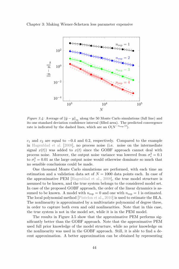
Chapter 3: Making Wiener-Schetzen less parameter expensive
103 104 10510−4
10−2
100
102
nrep = 1
nrep = 2
nrep = 3
nrep = 4
N
‖y−y‖ ∞
Figure 3.4: Average of ‖y − y‖∞ along the 50 Monte Carlo simulations (full line) andits one standard deviation confidence interval (filled area). The predicted convergencerate is indicated by the dashed lines, which are an O(N−nrep/2).
c1 and c2 are equal to −0.4 and 0.2, respectively. Compared to the examplein Hagenblad et al. [2008], no process noise (i.e. noise on the intermediatesignal x(t)) was added to x(t) since the GOBF approach cannot deal withprocess noise. Moreover, the output noise variance was lowered from σ2
v = 0.1to σ2
v = 0.01 as the large output noise would otherwise dominate so much thatno sensible conclusions could be made.
One thousand Monte Carlo simulations are performed, with each time anestimation and a validation data set of N = 1000 data points each. In case ofthe approximative PEM [Hagenblad et al., 2008], the true model structure isassumed to be known, and the true system belongs to the considered model set.In case of the proposed GOBF approach, the order of the linear dynamics is as-sumed to be known. A model with nrep = 0 and one with nrep = 1 is estimated.The local polynomial method [Pintelon et al., 2010] is used to estimate the BLA.The nonlinearity is approximated by a multivariate polynomial of degree three,in order to capture both even and odd nonlinearities. Note that in this case,the true system is not in the model set, while it is in the PEM model.
The results in Figure 3.5 show that the approximative PEM performs sig-nificantly better than the GOBF approach. Note that the approximative PEMused full prior knowledge of the model structure, while no prior knowledge onthe nonlinearity was used in the GOBF approach. Still, it is able to find a de-cent approximation. A better approximation can be obtained by representing
44

3.3 OBFs based on the poles of the BLA
0.3 0.4 0.5 0.6 0.7
0
100
200
300
400
500PEM, output noise
GOBF (0),output noise
GOBF (1),output noise
‖y(t)−y(t)‖2‖y(t)‖2
Nu
mb
erof
occ
urr
ence
s
Figure 3.5: Distribution of‖y(t)−y(t)‖2‖y(t)‖2
on the validation data sets for the 1000 Monte
Carlo simulations. PEM indicates the results for the approximative prediction errormethod, while GOBF (0) and GOBF (1) indicate the results for the proposed GOBFapproach with nrep = 0 and nrep = 1, respectively. For the parametric BLA, the av-
erage of‖y(t)−y(t)‖2‖y(t)‖2
along the 1000 Monte Carlo simulations is equal to 0.657, while
its standard deviation is equal to 0.0227.
the nonlinearity with another basis function expansion that is more appropriateto the nonlinearity at hand. Alternatively, support vector machines (SVMs)can be used [Totterman and Toivonen, 2009; Gomez and Baeyens, 2012].
Example 3: noisy case with polynomial nonlinearity
To make a fair comparison, the second example is modified such that the systemis in the model class for both of the considered approaches. The nonlinearityin (3.6) is changed to a third-degree polynomial that best approximates thesaturation nonlinearity on all the estimation data sets. The approximative PEMnow estimates a third-degree polynomial nonlinearity. In this case, the GOBFapproaches have a similar performance as the approximative PEM approach(see Figure 3.6).
To determine the number of required repetitions nrep, one can easily estimateseveral models for an increasing nrep, and compare the simulation errors on avalidation data set. Once the simulation error increases, the variance erroroutweighs the model error, and one should select less repetitions. Here, thenormalized rms error for nrep = 0 is lower than the normalized rms error fornrep = 1 in 850 out of the 1000 cases. A Wiener-Schetzen model with nrep = 0should then be selected, which corresponds to a model with 35 parameters.In the remaining 150 cases, one would select a model with nrep ≥ 1, whichcorresponds to a Wiener-Schetzen model with (at least) 120 parameters.
45

Chapter 3: Making Wiener-Schetzen less parameter expensive
0.3 0.32 0.34 0.36 0.38 0.4 0.42 0.44 0.46
0
100
200
300
PEM,output noise
GOBF (0),output noise
GOBF (1),output noise
‖y(t)−y(t)‖2‖y(t)‖2
Nu
mb
erof
occ
urr
ence
s
Figure 3.6: Distribution of‖y(t)−y(t)‖2‖y(t)‖2
on the validation data sets for the 1000 Monte
Carlo simulations (polynomial nonlinearity). For the parametric BLA, the average
of‖y(t)−y(t)‖2‖y(t)‖2
along the 1000 Monte Carlo simulations is equal to 0.566, while its
standard deviation is equal to 0.0410.
3.3.5 Conclusion
The input/output behavior of a Wiener system with finite-order IIR dynamicsand a polynomial nonlinearity can be well approximated by a Wiener-Schetzenmodel. The modeled output was shown to converge in probability to the trueoutput when GOBFs are used that are constructed based on the poles of theBLA of the system. A mismatch between the true and the estimated poles canbe handled by periodically repeating the set of pole estimates. Fast convergencerates, in terms of the number of required repetitions, can be obtained. Thisresults in Wiener-Schetzen models with a moderate number of parameters.
The approach can be applied to parallel Wiener systems as well.
3.4 The BLA as a basis function
Based on Tiels et al. [2012b] and Tiels et al. [2012a].
This section considers the approximation of single-branch Wiener systemswith Wiener-Schetzen models. It was shown in the previous section that by us-ing high-quality pole estimates the number of required repetitions of these poleestimates could be kept small. Nevertheless, the number of parameters can stillbe relatively large. This is because at least one basis function is needed forevery pole estimate, and the number of parameters increases combinatoriallywith the number of OBFs (see Table 1.1). Therefore, an extra parameter re-
46

3.4 The BLA as a basis function
duction step is proposed that is added to the identification procedure presentedin Subsection 3.3.2.
3.4.1 Basic idea
Since the asymptotic BLA (N →∞) is proportional to G(q) (special case ofTheorem 2.7), and considering that an arbitrary non-zero scaling factor can beexchanged between the linear and the nonlinear block of the Wiener system(see Figure 3.2), we propose to replace one of the OBFs by the estimated BLA.In that way, most of the dynamics are represented by only one basis function.The other basis functions can then be considered as correction terms, and manyof the parameters resulting from these other basis functions can be consideredsmall compared to those resulting from the BLA.
3.4.2 Parameter reduction step
Based on Tiels et al. [2012b].
This parameter reduction step is developed in more detail in this subsection.
Independent set of functions
Let GBLA(q, θ) be the transfer function representation of the parametric esti-
mate of the BLA GM (k, θ) in (3.2). By construction, GBLA(q, θ) is a linearcombination of the first np GOBFs, possibly augmented with a feed-throughterm:
GBLA(q, θ) =
np∑
i=0
ciFi(q) .
As a consequence, the set GBLA(q, θ), F0(q), . . . , Fn(q) does not constitute anindependent set of functions. To obtain an independent set again, it is necessaryto leave out one of the basis functions F0, . . . , Fnp . Since we want the BLA torepresent most of the dynamics and the other basis functions to correspond tosmall correction terms, we leave out the basis function Fi corresponding to themaximum absolute value of ci. Of all basis functions F0, . . . , Fnp , this Fi isthe one that contributes the most in the representation of the dynamics. Otherchoices on which basis function to leave out are tested in Subsection 3.4.4, whereit is observed that the choice is not really important. This is likely due to thefollowing orthogonalization step.
Orthonormal set of functions
The set GBLA(q, θ), F0(q), . . . , Fi−1(q), Fi+1(q), . . . , Fn(q) is not an orthonor-mal set of functions. One reason why we would like to obtain an orthonormal
47

Chapter 3: Making Wiener-Schetzen less parameter expensive
F⊥0 (q) ∝ GBLA(q, θ)
...
F⊥n (q)
f r(x⊥ 0,...,x⊥ n)
u(t)
x⊥0 (t) = x⊥BLA(t)
x⊥n (t)
y(t)
Figure 3.7: A Wiener-Schetzen model where the first OBF is proportional to theparametric estimate of the BLA (F⊥0 ∝ GBLA(q, θ), F⊥1 , . . . , F
⊥n is a set of OBFs
and fr is a multivariate polynomial).
set is the improved numerical conditioning of the parameter estimation. Anorthonormal set can be easily obtained by using the Gram-Schmidt procedure,resulting in the orthonormal set F⊥0 ∝ GBLA(q, θ), F⊥1 , . . . , F
⊥n . The model
structure shown in Figure 3.7 is obtained.
Parameter reduction
Define x⊥i as the output of the filter F⊥i (i = 0, . . . , n), and let x⊥0 = x⊥BLA.
In the model in Figure 3.7, fr is again a multivariate polynomial, but unlikebefore, it does not contain all possible terms x⊥i1 · · ·x⊥id . Since we consider x⊥ik ,
for ik 6= 0, to be a correction term, we keep only those terms x⊥i1 · · ·x⊥id in which
at most one factor x⊥ik 6= x⊥BLA is present:
fr(x⊥0 = x⊥BLA, x
⊥1 , . . . , x
⊥n ) = βrDC
+
D∑
d=1
n∑
i=0
βr BLA···BLA︸ ︷︷ ︸(d − 1) times
i(x⊥BLA)d−1x⊥i
.
In that way, the number of parameters is reduced from (see also Table 1.1)
nβ =(n+ 1 +D)!
(n+ 1)!D!
to
nβr = 1 +D(n+ 1) .
Note that the number of parameters now increases proportionally with thenumber of OBFs instead of combinatorially. This allows for a major reductionof the number of parameters, especially if the number of OBFs is large.
48

3.4 The BLA as a basis function
G1(q)
G2(q)
f(x1, x2)
u1(t)
u2(t)
x1(t)
x2(t)
y0(t)
Figure 3.8: A discrete-time TISO Wiener system (G1(q) and G2(q) are discrete-timelinear dynamic systems, f(x1, x2) is a bivariate static nonlinear function).
3.4.3 Extension to MISO single-branch Wiener systems
Based on Tiels et al. [2012a].
The identification procedure in Subsection 3.3.2 is extended to MISO Wienersystems in this subsection. As the number of parameters can increase signif-icantly compared to the SISO case, the parameter reduction step in Subsec-tion 3.4.2 is extended to MISO single-branch Wiener systems. The poles of theGOBFs will now be determined from an extension of the BLA towards multi-ple input multiple output (MIMO) systems [Dobrowiecki and Schoukens, 2007].To keep the notation as simple as possible, and without loss of generality, thenumber of inputs nu is restricted to two. As such, the identification of a TISO(two input single output) Wiener system (see Figure 3.8) is considered. TheTISO Wiener-Schetzen model is shown in Figure 3.9.
Estimation of an extension of the BLA towards MIMO systems
The BLA is extended to MIMO systems in Dobrowiecki and Schoukens [2007].For the TISO Wiener system shown in Figure 3.8, one obtains, similarly to (2.7)and Theorem 2.7,
Y0(k) = GBLA1(k)U1(k) +GBLA2(k)U2(k) + YS(k)
= cBLA1G1(k)U1(k) + cBLA2
G2(k)U2(k) + YS(k) +O(N−1) ,
where GBLA1and GBLA2
are the BLAs in the first and the second input/outputpath, respectively, YS is the nonlinear noise source, and cBLA1
and cBLA2are
constants that depend upon the odd nonlinearities in f(x1, x2) and the powerspectrum of the excitation signals u1(t) and u2(t).
In Dobrowiecki and Schoukens [2007], an optimized measurement strategyinvolving orthogonal random-phase multisine excitations is proposed to reduceas much as possible the influence of the nonlinear noise source YS on the es-timated BLA. Since YS acts as output noise, its influence can be reduced byaveraging over multiple experiments [Dobrowiecki et al., 2006] using each timea different realization of the random input signals.
49

Chapter 3: Making Wiener-Schetzen less parameter expensive
F1,0(q)
...
F1,n1(q)
F2,0(q)
...
F2,n2(q)
f(x
1,0,...,x
1,n
1,x
2,0,...,x
2,n
2)u1(t)
x1,0(t)
x1,n1(t)
u2(t)
x2,0(t)
x2,n2(t)
y(t)
Figure 3.9: A TISO Wiener-Schetzen model (F1,1(q), . . . , F1,n1(q) andF2,1(q), . . . , F2,n2(q) are GOBFs, F1,0(q) and F2,0(q) are feed-through terms,f(x1,0, . . . , x2,n2) is a multivariate polynomial function).
Assume that nexp different experiments are performed:
Y (k) = GBLA(k)U(k) + Y S(k) ,
with
Y (k) =[Y
[1]0 (k) . . . Y
[nexp]0 (k)
],
GBLA(k) =[GBLA1
(k) GBLA2(k)],
U(k) =
[U
[1]1 (k) . . . U
[nexp]1 (k)
U[1]2 (k) . . . U
[nexp]2 (k)
],
Y S(k) =[Y
[1]S (k) . . . Y
[nexp]S (k)
].
The idea proposed in Dobrowiecki et al. [2006] is to perform an integer numbernblocks of nu experiments (nexp = nblocksnu) and to use orthogonal random-phase multisines in each of the nblocks experiment blocks. For the TISO case
50

3.4 The BLA as a basis function
(nu = 2), the following series of experiments is proposed:
U i(k) =
[U
[2i−1]1 (k) U
[2i]1 (k)
U[2i−1]2 (k) U
[2i]2 (k)
]
=
[1 11 −1
]U
[2i−1]1 (k)
for i = 1, . . . , nblocks , (3.7)
where U[2i−1]1 (k) is the DFT spectrum of a random-phase multisine (see Defi-
nition 2.3). The nonparametric BLAs are then estimated as
Y i(k) =[Y
[2i−1]0 (k) Y
[2i]0 (k)
],
Gi(k) =[G
[i]BLA1
(k) G[i]BLA2
(k)]
= Y i(k)U−1i (k) ,
GBLA(k) =[GBLA1
(k) GBLA2(k)]
=1
nblocks
nblocks∑
i=1
Gi(k) .
Next, parametric models GM (k, θ1) and GM (k, θ2) of orders np1 and np2(to be chosen by the user) are identified on GBLA1
(k) and GBLA2(k) using
the weighted least-squares estimator in (3.2). Their poles p11 , . . . , p1np1and
p21 , . . . , p2np2are calculated.
Construct the GOBFs
These pole estimates are then used to construct two sets of OBFs: one setof OBFs F1,0, . . . , F1,n1 based on the pole estimates p11 , . . . , p1np1
and one
set of OBFs F2,0, . . . , F2,n2 based on the pole estimates p21
, . . . , p2np2(see
Figure 3.9).
Estimate the multivariate polynomial coefficients
Finally, the coefficients of the multivariate polynomial f are estimated. Definexi1,i2 as the output of the OBF Fi1,i2 (i1 = 1, 2; i2 = 0, . . . , ni1) and rename theoutputs to w0 = x1,0, . . . , wn1 = x1,n1 , wn1+1 = x2,0, . . . , wn = wn1+1+n2 = x2,n2 .The coefficients β of the multivariate polynomial
f(w0, . . . , wn,β) = βDC +
D∑
d=1
n∑
i1=0
n∑
i2=i1
· · ·n∑
id=id−1
βi1···idwi1 · · ·wid
51

Chapter 3: Making Wiener-Schetzen less parameter expensive
of degree D (to be chosen by the user), are estimated by solving the linearleast-squares problem
β = arg minβ
MSE(f(w0, . . . , wn,β)) ,
in which the (possibly weighted) mean-square error MSE is equal to
MSE =1
N
N−1∑
t=0
[y(t)− f(w0(t), . . . , wn(t),β)]2 .
Again, the number of parameters is equal to
nβ =(n+ 1 +D)!
(n+ 1)!D!. (3.8)
Parameter reduction step in the MISO case
The number of parameters increases again combinatorially with the numberof inputs to the multivariate polynomial. This number can rapidly becomelarge, especially for MISO systems. Therefore, the parameter reduction step inSubsection 3.4.2 is extended to the MISO case.
The representation of the TISO Wiener system in Figure 3.8 is not unique.Arbitrary non-zero constants ceq1
and ceq2can be exchanged between the linear
blocks and the nonlinear block (see Figure 3.10). Hence, we propose to replaceone OBF in each input/output path by the estimated BLA in that path. Likethis, a large portion of the dynamics in each input/output path is captured byonly one basis function. The remaining basis functions will again be consideredas correction terms. This will reduce the number of significantly contributingparameters.
Let GBLAi1(q, θi1) be the transfer function model that corresponds to the
parametric estimate of the BLA GM (k, θi1) in the i1th input/output path.
First, one of the OBFs Fi1,0(q), . . . , Fi1,npi1(q) is replaced by GBLAi1
(q, θi1)
in each input/output path to obtain independent sets of functions. Next, theGram-Schmidt procedure is applied to each of the obtained sets of functions toobtain orthonormal sets of functions F⊥i1,0 ∝ GBLAi1
(q, θi1), F⊥i1,1, . . . , F⊥i1,ni1
in each input/output path. In each of these sets, the first OBF is proportional tothe BLA in that input/output path. Finally, the coefficients of the multivariate
polynomial fr in Figure 3.11 are estimated. Define x⊥i1,i2 as the output of the
filter F⊥i1,i2 (i1 = 1, 2; i2 = 0, . . . , ni1), let x⊥i1,0 = x⊥BLAi1, and rename the out-
puts to w⊥0 = x⊥1,0, . . . , w⊥n1
= x⊥1,n1, w⊥n1+1 = x⊥2,0, . . . , w
⊥n = w⊥n1+1+n2
= x⊥2,n2.
The polynomial fr does not contain all possible terms of degree at most D.
52

3.4 The BLA as a basis function
ceq1G1(q)
ceq2G2(q)
f(x1
ceq1, x2
ceq2
)u1(t)
u2(t)
ceq1x1(t)
ceq2x2(t)
y0(t)
Figure 3.10: Arbitrary non-zero scaling factors ceq1 and ceq2 can be exchanged betweenthe linear dynamic blocks and the static nonlinear block in the TISO Wiener systemin Figure 3.8, without changing the input/output behavior of the system.
Since we consider w⊥ik , for ik 6= 0, n1 + 1, to be correction terms, we keep only
those terms in which at most one factor w⊥ik 6= x⊥BLA1, x⊥BLA2
is present. Inthat way, the number of parameters no longer increases combinatorially withthe number of inputs to the polynomial as in (3.8). The number of parametersis reduced to
nβr =(D + 2)(D + 1)
2+ (n− 1)
(D + 1)D
2,
and hence only increases proportionally with n. In the general case of nu inputs,the number of parameters is reduced to (see Appendix 3.F)
nβr =(nu +D)!
nu!D!+ (n+ 1− nu)
(nu +D − 1)!
nu!(D − 1)!. (3.9)
3.4.4 Illustration
This subsection illustrates the proposed parameter reduction step on two simu-lation examples. The first one considers the SISO case, the second one considersthe TISO case. The choice on which basis function to leave out when construct-ing an independent set of functions is also examined in the SISO case.
Example 1: the SISO case
Based on Tiels et al. [2012b].
Consider a SISO discrete-time Wiener system (see Figure 3.1). The lineardynamic system G(q) is a third-order low-pass Chebyshev Type I filter with10 dB peak-to-peak ripple in the passband and with a normalized passband edgefrequency ωp = 0.2846. Its FRF is shown in Figure 3.12. The static nonlinearfunction f(x) = x+ 0.8x2 + 0.7x3 is a third-degree polynomial. No noise isadded to the output in order to focus completely on the model errors.
The system is excited by a random-phase multisine signal u(t) containingN = 8192 samples. The excited frequencies are equidistantly spaced between
53

Chapter 3: Making Wiener-Schetzen less parameter expensive
F⊥1,0(q) ∝ GBLA1(q, θ1)
...
F⊥1,n1(q)
F⊥2,0(q) ∝ GBLA2(q, θ2)
...
F⊥2,n2(q)
f r(x⊥ 1,0,...,x⊥ 1,n
1,x⊥ 2,0,...,x⊥ 2,n
2)u1(t)
x⊥1,0(t) = x⊥BLA1(t)
x⊥1,n1(t)
u2(t)
x⊥2,0(t) = x⊥BLA2(t)
x⊥2,n2(t)
y(t)
Figure 3.11: A TISO Wiener-Schetzen model where the first OBF in each in-put/output path is proportional to the parametric estimate of the BLA in that path(F⊥1,0 ∝ GBLA1(q, θ1), F⊥1,1, . . . , F
⊥1,n1 and F⊥2,0 ∝ GBLA2(q, θ2), F⊥2,1, . . . , F
⊥2,n2 are
sets of OBFs and fr is a multivariate polynomial).
DC and one sixth of the sample frequency, which is normalized to fs = 1 Hz.Within this range, the amplitudes |Uk| are chosen equal to each other and suchthat the rms value of u(t) is equal to one. One hundred phase realizationsof the multisine are applied for estimation purposes, although much less phaserealizations would suffice. One extra phase realization of the multisine is appliedto do the validation.
The system is identified using the identification procedure described in Sub-section 3.3.2, once including the parameter reduction step described in Sub-section 3.4.2 and once not including this extra step. The BLA of the systemis estimated by averaging out the division of the output and the input spec-trum over the one hundred phase realizations of the multisine. On top of thisnonparametric estimate, a parametric model of order np = 3 is identified. The
coefficients of the multivariate polynomials f and fr are estimated using thefirst phase realization of the multisine that was used to identify the BLA.
Table 3.1 shows the number of parameters and the relative rms error on thesimulated output as a function of the number of OBFs. The relative rms error
54

3.4 The BLA as a basis function
is calculated as
relative rms error =
√1N
∑N−1t=0 (y(t)− y(t))2
√1N
∑N−1t=0 y2(t)
.
When the parameter reduction step is not included, the rms error can be madearbitrarily small by increasing the number of OBFs. This is not the case whenthe parameter reduction step is included. In this case, the rms error decreaseswhen increasing the number of OBFs from (n+ 1) = 4 to (n+ 1) = 10. Fur-ther increasing the number of OBFs does not decrease the rms error. Up to(n+ 1) = 7, the rms error is more or less the same, whether the parameter re-duction step is included or not. However, when this extra step is included, thenumber of parameters is significantly smaller.
For the case (n+ 1) = 7, Figure 3.13 compares the magnitude of the param-eters, i.e. the polynomial coefficients, when all of the 120 possible monomials inx⊥0 = x⊥BLA, x⊥1 , . . . , x⊥6 up to third degree are considered and the magnitude of
the parameters when only the a priori selected monomials in fr are considered.In this comparison, the orthogonal regressors are normalized to have unit rmsvalue, so that the magnitude of the parameters indicates the contribution of thecorresponding term to the rms value of the output. It can be observed that theparameters corresponding to terms that include at least two correction termscan indeed be neglected.
To examine the influence of which basis function is left out in the parameterreduction step (see Subsection 3.4.2), each of the options is checked. Theseoptions are the basis functions F0, . . . , Fnp . For each of these options, the samerelative rms errors are obtained, while the condition number of the parameterestimation only slightly differs (see Table 3.2). We can conclude that the choiceof which OBF is left out does not really matter. This is likely due to theorthogonalization step. Independent of which basis function is left out initially,sets of orthonormal basis functions with the same span are obtained.
Example 2: the TISO case
Based on Tiels et al. [2012a].
Consider the TISO discrete-time Wiener system in Figure 3.8. The lineardynamic systems G1(q) and G2(q) are second-order low-pass Chebyshev Type Ifilters, the former with 10 dB peak-to-peak ripple in the passband and with anormalized passband edge frequency ωp1 = 0.1, the latter with 20 dB peak-to-peak ripple in the passband and with a normalized passband edge frequencyωp1 = 0.2. The static nonlinear function
f(x1, x2) = x1 +x2 +0.5x21 +0.2x1x2 +0.5x2
2 +0.2x31 +0.1x2
1x2 +0.1x1x22 +0.2x3
2
55

Chapter 3: Making Wiener-Schetzen less parameter expensive
0 16
0.25 0.5−100
−50
−20
−10
0
Frequency (Hz)
Am
pli
tud
e(d
B)
Figure 3.12: FRF of the linear dynamic system G(q) in the SISO Wiener systemdescribed in Subsection 3.4.4.
is a third-degree bivariate polynomial. A plot of this function is shown inFigure 3.14. Again, no noise is added to the output to focus on the modelerrors.
The excitation signals u1(t) and u2(t) are random-phase multisines contain-ing N = 512 samples. The excited frequencies are between DC and one sixth ofthe sample frequency. Within this range, the multisines have a flat amplitudespectrum. Their rms value is equal to one. Ten experiment blocks accordingto (3.7) are applied to do the estimation. One extra phase realization of themultisines is applied to do the validation.
The system is identified using the identification procedure described in Sub-section 3.4.3, once including the parameter reduction step and once not in-cluding this extra step. The parametric models of the BLAs are of ordernp1 = np2 = 2. The coefficients of the multivariate polynomials f and fr, whichare polynomials of degree D = 3, are estimated using the data of all ten exper-iment blocks.
Figure 3.15 shows the FRFs of the true and the estimated linear dynamics.It can be observed that GBLA1
(q, θ1) and GBLA2(q, θ2) can describe much of the
dynamics in their respective input/output path. This motivates the parameterreduction step.
Table 3.3 shows the number of parameters and the relative rms error on thesimulated output as a function of the number of OBFs in each input/output
56

3.4 The BLA as a basis function
Table 3.1: Number of parameters nβ (without parameter reduction step) and nβr(with parameter reduction step), and relative rms error on the simulated output (withand without parameter reduction step) as a function of the number of OBFs n+ 1.
n+ 1 nβ nβrRelative rms error (in dB)
Without parameter reduction With parameter reduction
4 35 13 −55 −557 120 22 −110 −109
10 286 31 −165 −11513 560 40 −220 −11516 969 49 −274 −115
0 20 40 60 80 100 120−200
−150
−100
−50
0
Parameter
Mag
nit
ud
e(d
B)
Figure 3.13: Magnitude of the parameters when all possible monomials are selected(blue) and when only the monomials with at most one correction term are selected(green) for the case (n+ 1) = 7. The first parameter indicated in green correspondsto the DC value, the next three to x⊥BLA, (x⊥BLA)2, and (x⊥BLA)3, the next six to(x⊥BLA)2x⊥1 , . . . , (x⊥BLA)2x⊥6 , the next six to x⊥BLAx
⊥1 , . . . , x⊥BLAx
⊥6 , and the final six
to x⊥1 , . . . , x⊥6 . The parameters that only have an indication in blue correspond tomonomials with at least two correction terms.
57
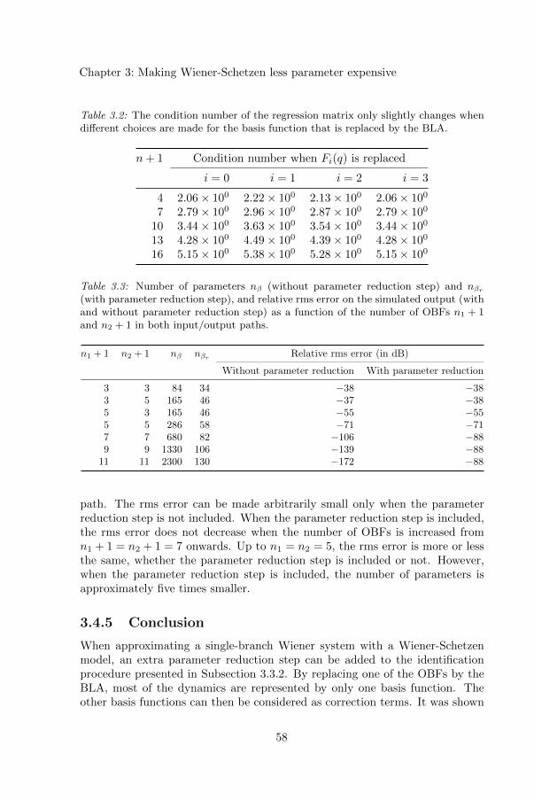
Chapter 3: Making Wiener-Schetzen less parameter expensive
Table 3.2: The condition number of the regression matrix only slightly changes whendifferent choices are made for the basis function that is replaced by the BLA.
n+ 1 Condition number when Fi(q) is replaced
i = 0 i = 1 i = 2 i = 3
4 2.06× 100 2.22× 100 2.13× 100 2.06× 100
7 2.79× 100 2.96× 100 2.87× 100 2.79× 100
10 3.44× 100 3.63× 100 3.54× 100 3.44× 100
13 4.28× 100 4.49× 100 4.39× 100 4.28× 100
16 5.15× 100 5.38× 100 5.28× 100 5.15× 100
Table 3.3: Number of parameters nβ (without parameter reduction step) and nβr(with parameter reduction step), and relative rms error on the simulated output (withand without parameter reduction step) as a function of the number of OBFs n1 + 1and n2 + 1 in both input/output paths.
n1 + 1 n2 + 1 nβ nβr Relative rms error (in dB)
Without parameter reduction With parameter reduction
3 3 84 34 −38 −383 5 165 46 −37 −385 3 165 46 −55 −555 5 286 58 −71 −717 7 680 82 −106 −889 9 1330 106 −139 −88
11 11 2300 130 −172 −88
path. The rms error can be made arbitrarily small only when the parameterreduction step is not included. When the parameter reduction step is included,the rms error does not decrease when the number of OBFs is increased fromn1 + 1 = n2 + 1 = 7 onwards. Up to n1 = n2 = 5, the rms error is more or lessthe same, whether the parameter reduction step is included or not. However,when the parameter reduction step is included, the number of parameters isapproximately five times smaller.
3.4.5 Conclusion
When approximating a single-branch Wiener system with a Wiener-Schetzenmodel, an extra parameter reduction step can be added to the identificationprocedure presented in Subsection 3.3.2. By replacing one of the OBFs by theBLA, most of the dynamics are represented by only one basis function. Theother basis functions can then be considered as correction terms. It was shown
58

3.5 Iterative update of the pole locations
−0.5 00.5 1
−0.5
00.5
0
2
4
x1x2
f(x
1,x
2)
Figure 3.14: Plot of the bivariate polynomial f(x1, x2) considered in Example 2 inSubsection 3.4.4.
that in this way, the number of relevantly contributing terms in the multivariatepolynomial is significantly reduced. Instead of a combinatorial increase of thenumber of parameters with the number of OBFs, a proportional increase isobtained. The identification method and the extra parameter reduction stepwere extended to the multiple input case.
3.5 Iterative update of the pole locations
Based on Tiels and Schoukens [2013b].
This section considers again the approximation of (parallel) Wiener systemswith Wiener-Schetzen models, and proposes an alternative parameter reductionstep. As shown in Section 3.3, a mismatch between the true and the estimatedpoles can be handled by periodically repeating the set of pole estimates. Byusing high-quality pole estimates, the number of pole repetitions can be keptsmall, resulting in a Wiener-Schetzen model with a moderate number of pa-rameters. Here, we propose an iterative scheme to improve the quality of thepole estimates, without making repeated measurements, so that eventually thenumber of pole repetitions can be reduced, and as such also the number ofparameters.
59

Chapter 3: Making Wiener-Schetzen less parameter expensive
0 0.05 0.1 0.15−40
−30
−20
−10
0
10
Frequency (Hz)
Am
pli
tud
e(d
B)
G1
GBLA1
GBLA1G1
(a) First input/output path
0 0.05 0.1 0.15−40
−30
−20
−10
0
10
Frequency (Hz)
Am
pli
tud
e(d
B)
G2
GBLA2
GBLA2G2
(b) Second input/output path
Figure 3.15: FRFs of the true (G1(q) and G2(q)) and the estimated (GBLA1(q, θ1)and GBLA2(q, θ2)) linear dynamics in the TISO Wiener system described in Subsec-tion 3.4.4.
60

3.5 Iterative update of the pole locations
data
BLA
pole estimates
GOBFs
nonlinearity
Wiener-Schetzenmodel
Figure 3.16: Schematic overview of the proposed iterative update scheme.
3.5.1 Basic idea
A schematic overview of the proposed iterative scheme is shown in Figure 3.16.Since an increased number of GOBFs compensates for the mismatch betweenthe true and the estimated poles, a high-order Wiener-Schetzen model is firstestimated. In each iteration, a nonparametric BLA is calculated analyticallyon the Wiener-Schetzen model obtained in the previous iteration. Next, a low-order parametric BLA is estimated on the non-parametric one, and its polesare calculated. With these pole estimates, the GOBFs are constructed. Thenonlinearity is estimated on the measured input/output data, which resultsin a new estimate of the high-order Wiener-Schetzen model. The scheme isinitialized with a nonparametric BLA estimate, calculated from the measuredinput/output data.
The idea of first estimating a high-order model and next extracting a low-order model from it is not new. A similar approach for the LTI setting isdescribed in Akcay and Heuberger [2001]. There, a high-order transfer func-tion model on the basis of GOBFs is estimated from the data and a low-ordermodel is extracted via optimal Hankel norm model reduction. Here, the idea isextended to the class of Wiener systems.
3.5.2 Causes for pole mismatch
This subsection analyzes the measured and the modeled output spectrum, andas such reveals the causes for the mismatch between the true poles and thoseestimated via the BLA. Each of these causes is tackled in the next subsection.
To keep the notation as simple as possible, a single-branch discrete-timeWiener system as in Figure 3.1 is considered with f(x) = x3. Nevertheless, theideas can be generalized to parallel Wiener systems and a polynomial represen-
61

Chapter 3: Making Wiener-Schetzen less parameter expensive
tation of the static nonlinearity of arbitrary degree.Since the input is chosen to be periodic (see Subsection 3.2.2), the BLA
is estimated by averaging out Y (k)U(k) over a number of phase realizations of the
multisine (see also (2.9)).
Measured output spectrum
A multiplication in the time domain corresponds to a convolution in the fre-quency domain. The true, noise-free, output spectrum of the Wiener system inFigure 3.1 with f(x) = x3 is thus equal to
Y0(k) =1
N
N/2∑
l1,l2,l3=−N/2+1
X(l1)X(l2)X(l3) , (3.10)
with∑3i=1 li = k.
Some of the terms in Y0(k) sum up to the output spectrum of the BLA. Theseare the terms where one of the lis is equal to k, and where the two other factorsin the product X(l1)X(l2)X(l3) combine pairwise to X(l)X(−l) = |X(l)|2 (seealso Appendix 2.A). These terms sum up to
YBLA(k) =1
N
N/2∑
l=−N/2+1
∑
perm(k,l,−l)X(k)|X(l)|2 , (3.11)
where the second sum runs over all permutations of (k, l,−l) [Pintelon andSchoukens, 2012]. Thus
YBLA(k) =1
NX(k)
N/2∑
l=−N/2+1l 6=k
6|X(l)|2
+ 3|X(k)|2
= G(k)U0(k)
1
N
N/2∑
l=−N/2+1
6|X(l)|2− 1
N3|X(k)|2
=(cBLAG(k) +O(N−1)
)U0(k) .
(3.12)
The bias on the BLA, which is an O(N−1), thus originates in this case from thedifference between the number of permutations of (k, l,−l) and the number ofpermutations of (k, k,−k).
The remaining terms in (3.10) that do not contribute to YBLA sum up to
the nonlinear noise source YS . When averaging Y (k)U(k) out over a finite number of
62

3.5 Iterative update of the pole locations
phase realizations, Ys does have a non-zero contribution that behaves as noisedue to the random behavior of the input.
Since the output measurement is corrupted by measurement noise v(t), themeasured output spectrum is given by
Y (k) = YBLA(k) + YS(k) + V (k)
=(cBLAG(k) +O(N−1)
)U0(k) + YS(k) + V (k) .
(3.13)
Modeled output spectrum
As shown in Theorem 3.11 and Subsection 3.3.3, the modeled output spectrumis equal to
Y (k) = Y0(k) +Op(N−nrep/2) +O(N−1/2) . (3.14)
The term Op(N−nrep/2) is due to pole mismatch. The term O(N−1/2) is due to
measurement noise and the stochastic nonlinearities YS that are present, evenin the absence of measurement noise.
Conclusion
From (3.13) and (3.14), we can conclude that the true BLA asymptoticallyresults in the true pole locations. If we want to retrieve the true pole locationsfrom the estimated BLA, we need to get rid of the nonlinear noise source YS andthe bias on the BLA. If not, a model error on the estimated output results thatis due to pole mismatch. Besides the above mentioned unwanted contributions,the measurement noise affects the modeled output spectrum as well.
3.5.3 Iterative update scheme
This subsection first discusses how to tackle each of the error sources. Thisleads to an iterative update scheme, which is presented next.
Tackling the nonlinear noise source
The nonlinear noise source YS has a zero mean with respect to the randomphases of the input. One possibility to reduce the magnitude of YS is thusto generate simulation data from the estimated Wiener-Schetzen model, andto estimate the BLA from this extra data. As the BLA estimate can then beaveraged over more phase realizations, the magnitude of YS drops towards zero.
An alternative is to calculate the BLA analytically on the estimated model.As in (3.10) for a single-branch Wiener system, one can calculate the BLAof a Wiener-Schetzen model by explicitly calculating the convolution in thefrequency domain. When taking into account only those terms that contribute
63

Chapter 3: Making Wiener-Schetzen less parameter expensive
to YBLA, as is done in (3.11) for the Wiener system, one gets completely rid ofthe nonlinear noise source YS .
Only the odd nonlinearities should be calculated, since it is impossible foreven nonlinearities to split of a factor X(k), while the other factors combinepairwise to contributions of the form X(l)X(−l) = |X(l)|2.
It should be mentioned that the number of calculations increases combina-torially with the degree of nonlinearity. Thus, the analytical calculation of theBLA should only be done in case of moderate degrees of nonlinearity, e.g. upto fifth-degree nonlinearities. For higher-degree nonlinearities, one can resortto BLA estimates on simulation data.
Tackling the bias on the BLA
In (3.12), the bias on the BLA originates from the difference between the numberof permutations of (k, l,−l) when l 6= k and when l = k. When accounting forthis during the analytical calculation of the BLA, for example in (3.12) bycounting the contributions X(k)|X(k)|2 twice, the bias on the BLA is removed.
Tackling the model error due to pole mismatch
As the first estimate of the Wiener-Schetzen model is initialized from the es-timated BLA, a model error due to pole mismatch is present in the modeledoutput spectrum. This model error is an Op(N
−nrep/2) and thus its magnitudedecreases when more pole repetitions are used. For that reason, a high-orderWiener-Schetzen model is estimated, i.e. nrep > 1. On this model, the BLA iscalculated analytically. Intuitively, one would expect improved pole estimatesfrom this BLA, since the increased number of basis functions compensates forthe pole mismatch. The scheme is thus repeated iteratively, until the totalmodel error is below a user-specified level, or until it reaches the lower boundthat is set by the disturbing noise.
Tackling the measurement noise
The measurement noise v(t) is present in the measured data. Its influencecannot be nullified, but it can be reduced in two ways.
As the data is assumed to be periodic, the input and output spectrum canbe averaged over several periods. The measurement noise gets averaged out anddrops towards zero at a cost of an increased measurement time.
The noise sensitivity of a model is larger if it contains a larger number ofparameters. Therefore, nrep = 2 will be used. Like this, a compensation for thepole mismatch is present, while the noise sensitivity of the estimated model isminimal.
64

3.5 Iterative update of the pole locations
Iterative scheme
The measures that have been taken to get rid of the error sources result in aniterative update scheme (see Figure 3.16). First, a high-order (with nrep = 2)Wiener-Schetzen model is estimated using the identification procedure describedin Subsection 3.3.2. As long as the obtained model is unsatisfactory, a low-orderBLA of the model is analytically calculated as described above, and a new high-order Wiener-Schetzen model is estimated, this time using the pole estimatesof the calculated low-order BLA.
With the improved pole estimates, one could estimate a lower-order Wiener-Schetzen model (nrep = 1) that clearly contains a smaller number of parameters.
3.5.4 Illustration
This subsection illustrates the iterative update scheme on a simulation example.Three situations are considered: the noise-free case, the noisy case, and the casewhere the model order is unknown.
Setup
Consider the discrete-time Wiener system given by (3.4) and (3.5). The systemis excited with an odd random-phase multisine containing N = 1024 samples.The excited frequencies are between DC and one sixth of the sample frequency.Only odd frequencies are excited. The amplitudes |Uk| of the excited frequenciesare chosen equal to each other and such that the rms value of u(t) is equal toone. An odd random-phase multisine is chosen to get rid of the even nonlineardistortions in the BLA estimate. Two phase realizations and P = 2 periods areapplied for estimation purposes.
Example 1: noise-free case
First, consider the noise-free case. Fifty Monte Carlo simulations are performed,with each time a different realization of the random phases of the multisine.
Figure 3.17 shows ρ (see (2.17)), which can be interpreted as a measure forthe quality of the pole estimates, as a function of the iteration number. Thecloser ρ is to zero, the closer the pole estimates ξi are to the true pole locationspk of the underlying linear dynamic system. Figure 3.18 shows the relative rmserror on the simulated output for a validation data set that was not used duringidentification.
The results show that the proposed method converges in this case (a Wienersystem with a polynomial nonlinearity) to the true poles on a finite noiselessdata set. Only a few iterations are needed.
65

Chapter 3: Making Wiener-Schetzen less parameter expensive
1 2 3 4 5 6 7 8 9 10
−300
−200
−100
0
Iteration number
ρ(d
B)
medianmean
Figure 3.17: (Example 1) The median and the mean of ρ, a quality measure of thepole estimates, along the 50 Monte Carlo simulations. The minimum and maximum ρfor each iteration number correspond to the lower and upper bound of the filled grayarea. The bounds of the gray area thus indicate the best and worst case. From thefifth iteration on, the minimum is ρ = 0.
1 2 3 4 5 6 7 8 9 10
−300
−200
−100
0
Iteration number
Rel
ativ
erm
ser
ror
(dB
)
medianmean
Figure 3.18: (Example 1) The median and the mean of the relative rms error alongthe 50 Monte Carlo simulations. The minimum and maximum relative rms error foreach iteration number correspond to the lower and upper bound of the filled gray area.
66

3.5 Iterative update of the pole locations
1 2 3 4 5 6 7 8 9 10
−60
−40
−20
0
Iteration number
ρ(d
B)
medianmean
Figure 3.19: (Example 2) The median and the mean of ρ, a quality measure of thepole estimates, along the 50 Monte Carlo simulations. The minimum and maximum ρfor each iteration number correspond to the lower and upper bound of the filled grayarea. (Noisy case: SNRy = 20 dB)
Example 2: noisy case
Next, consider the case where the output measurement is corrupted with a
zero-mean white Gaussian noise. The output signal-to-noise ratio SNRy =σ2y0
σ2v
is chosen equal to 100. In each of the fifty Monte Carlo simulations, differentrealizations of the excitation signal and the output noise are generated.
The results in Figures 3.19 and 3.20 show that the iterative update schemefinds improved pole estimates, and that the relative rms error on the simulatedoutput reaches the noise floor. The measurement noise prevents the methodfrom retrieving the true poles. Note that a large gain can be made, especiallyin the worst-case, by running just a few iterations.
Example 3: unknown model order
Finally, consider the case where the model order is unknown. In this case, themodel order should be estimated on the nonparametric BLA estimate in theinitialization step. Several methods can be used for this purpose, such as theAIC criterion [Akaike, 1974], the MDL criterion [Rissanen, 1978], or variants ofthem [De Ridder et al., 2005].
Instead of estimating the model order, we here investigate the behavior of
67

Chapter 3: Making Wiener-Schetzen less parameter expensive
1 2 3 4 5 6 7 8 9 10−25
−20
−15
−10
−5
0
Iteration number
Rel
ativ
erm
ser
ror
(dB
)
medianmean
Figure 3.20: (Example 2) The median and the mean of the relative rms error alongthe 50 Monte Carlo simulations. The minimum and maximum relative rms error foreach iteration number correspond to the lower and upper bound of the filled gray area.The noise floor 1√
P
σvσy0
is at −23 dB. (Noisy case: SNRy = 20 dB)
the iterative update scheme if an incorrect model order is provided. We considerthe noisy case, where G(q) is believed to have five poles and five zeros (over-modeling), three poles and one zero (under-modeling 1), and two poles and twozeros (under-modeling 2). The results are shown in Figures 3.21 and 3.22.
In case the correct number of poles is estimated (under-modeling 1) or thetrue poles can be estimated (over-modeling with pole-zero cancellations), therelative rms error reaches the noise floor. Nevertheless, the pole estimates arebetter in case of over-modeling. When a too small number of poles is estimated,the method fails to improve the initial estimate.
3.5.5 Conclusion
An iterative update scheme for the pole locations in a Wiener-Schetzen modelwas presented. Instead of numerically optimizing both the pole locations andthe polynomial coefficients at the same time, the iteration is split into twosimpler steps: the estimation of a high-order Wiener-Schetzen model, and theextraction of a low-order BLA from the estimated Wiener-Schetzen model. Theonly nonlinear optimization step in this case is the estimation of a parametrictransfer function model, which is a well-studied problem. Moreover, no addi-
68

3.5 Iterative update of the pole locations
1 2 3 4 5 6 7 8 9 10−60
−40
−20
0
Iteration number
ρ(d
B)
medianmean
Figure 3.21: (Example 3) The median and the mean of ρ, a quality measure of thepole estimates, along the 50 Monte Carlo simulations. The minimum and maximum ρfor each iteration number correspond to the lower and upper bound of the filled area.(Model order 5/5: blue, 1/3: green, and 2/2: red)
1 2 3 4 5 6 7 8 9 10−25
−20
−15
−10
−5
0
Iteration number
Rel
ati
verm
ser
ror
(dB
)
medianmean
Figure 3.22: (Example 3) The median and the mean of the relative rms error alongthe 50 Monte Carlo simulations. The minimum and maximum relative rms error foreach iteration number correspond to the lower and upper bound of the filled area.(Model order 5/5: blue, 1/3: green, and 2/2: red)
69

Chapter 3: Making Wiener-Schetzen less parameter expensive
tional measurements are required for this method. A simulation example on aWiener system with a polynomial nonlinearity showed convergence to the truepole locations on a finite, noise-free data set. With the improved pole estimates,a lower-order Wiener-Schetzen model with a smaller number of parameters canbe estimated.
3.6 Overall conclusion
The approximation of the input/output behavior of a (parallel) Wiener systemwith that of a Wiener-Schetzen model is considered.
Prior knowledge of the linear dynamics in the Wiener system can be in-corporated in the Wiener-Schetzen model by constructing the OBFs based onuser-specified pole locations. A mismatch between the true and the specifiedpoles can be handled by periodically repeating the set of specified poles. Bychoosing the poles based on the BLA of the Wiener system, it was shown thatthe number of pole repetitions could be kept small, which results in a Wiener-Schetzen model with a moderate number of parameters.
The number of parameters can be reduced further for single-branch Wienersystems by using the BLA itself as a basis function. The remaining basis func-tions can then be considered as correction terms, which reduces the number ofsignificantly contributing parameters.
Another way to reduce the number of parameters in a Wiener-Schetzenmodel when approximating (parallel) Wiener systems is to iteratively improvethe pole estimates. In each iteration, a high-order Wiener-Schetzen model isestimated, and a low-order BLA is extracted. The improved pole estimatesremove the need for the periodic repetition of the pole estimates. Hence, one canestimate a low-order Wiener-Schetzen model, which contains less parameters.
70

3.A Normalized Q-polynomials
Appendix
3.A Normalized Q-polynomials
An ordinary multivariate polynomial in the variables x0, . . . , xn with all possibledth-degree terms can be represented as
y(t) =
n∑
i1=0
n∑
i2=i1
· · ·n∑
id=id−1
βi1,...,idxi1(t) · · ·xid(t) .
The coefficients β of the polynomial can be determined using a linear regression,where the terms xi1(t) · · ·xid(t) are the regressors. To improve the numericalconditioning of the estimation of the coefficients β, orthogonal regressors canbe used (see also Appendix 2.B). Hence, we replace the terms xi1 · · ·xid bymultivariate Hermite polynomials.
Multivariate Hermite polynomials are calledQ-polynomials in Schetzen [2006].The dth-degree Q-polynomial in the variables x0, . . . , xn is defined as
Q(d)i1i2...id
(x) =
n∏
i=0
Hni(xi) ,
where i1, . . . , id ∈ 0, . . . , n, and where ni, the degree of the Hermite polyno-mial of the variable xi, is equal to the number of times the integer i appears inthe subscript of Q.
If the variables x0, . . . , xn are statistically independent, i.e. orthogonal,Gaussian random variables with zero mean, which is for example the case if thevariables x0, . . . , xn are the outputs of OBFs with a white Gaussian input (seeSubsection 2.4.3), then it is shown in Schetzen [2006] that the Q-polynomialsare orthogonal. This means that
limT→∞
1
2T
∫ T
−TQ
(d1)i1i2...id1
(x(t))Q(d2)k1k2...kd2
(x(t)) dt
is zero whenever (i1, i2, . . . , id1) is not a permutation of (k1, k2, . . . , kd2). Sincewe use normalized Hermite polynomials (see Appendix 2.B), the Q-polynomialsare not only orthogonal, but also orthonormal.
3.B Proof of Lemma 3.9
Proof. Let θ be the “true” model parameters, such that
GM (k, θ) = cBLAG(k)
=Bθ(k)
Aθ(k)
∀ωk ,
71

Chapter 3: Making Wiener-Schetzen less parameter expensive
with Aθ and Bθ polynomials of degree np. The roots of Aθ(k) are equal to thetrue poles pi (i = 1, . . . , np). If these poles are all distinct, the first-order Taylorexpansion of Aθ(k) results in [Guillaume et al., 1989]
∆pi ≈ −na∑
l=0
pil
A′θ(pi)
∆al , (3.15a)
where A′
θ(pi) 6= 0, and where ∆al follows from
θ − θ =[∆a0 · · · ∆ana ∆b0 · · · ∆bnb
]T. (3.15b)
For a random-phase multisine excitation with finite power (see Definition 2.3),and under Assumptions 2.5 and 3.7, it is shown in Schoukens et al. [1998] that
plimN→∞
(θ(N)− θ
)= 0 .
For the considered output disturbances (no noise in Subsection 3.3.2, filteredwhite noise in Subsection 3.3.3), the least-squares estimator (3.2) is a maximumlikelihood estimator (MLE) [Pintelon et al., 1994]. From the properties of theMLE, it follows that [Pintelon and Schoukens, 2012]
θ = θ +Op(N−1/2) . (3.16)
Then from (3.15) and (3.16), it follows that
∆pi = Op(N−1/2) . (3.17)
This concludes the proof of Lemma 3.9.
3.C Proof of Lemma 3.10
Proof. From (2.17) and (3.17), it follows that ρ is an Op(N−1/2). It then follows
from (2.18) that G(q)−∑nl=0 αlFl(q) = Op(N
−nrep/2), and thus ∆x(t) is anOp(N
−nrep/2).
72

3.D Proof of Theorem 3.11
3.D Proof of Theorem 3.11
Proof. The exact output
y(t) =
D∑
d=0
γdxd(t)
=
D∑
d=0
γd
(n∑
l=0
αlxl(t) + ∆x(t)
)d
=
D∑
d=0
γd
(n∑
l=0
αlxl(t)
)d+ ∆y
= βDC +
D∑
d=1
n∑
i1=0
n∑
i2=i1
· · ·n∑
id=id−1
βi1,...,idxi1(t) · · ·xid(t)
+ ∆y(t)
= yβ(t) + ∆y(t) ,
where yβ(t) is the output of a multivariate polynomial f(x0, . . . , xn), in which
the coefficients β follow from the true coefficients γd of f(x) and the true coeffi-cients αl of the series expansion of G(q). The truncation of this series expansionis taken into account by the term ∆y(t), which just as ∆x(t) is an Op(N
−nrep/2).Note that the coefficients β can be obtained as the minimizers of the artificial
least-squares problemβ = arg min
β‖Jβ − yβ‖22 .
The estimated coefficients are equal to
β = (JTJ)−1JTy
= (JTJ)−1JT (yβ + ∆y)
= β + (JTJ)−1JT∆y .
(3.18)
We now show that (JTJ)−1JT∆y is an Op(N−nrep/2).
Each element in J is an O(N0), due to the normalization of the excitationsignal (see Subsection 3.2.2). Consequently, each element in the matrix JTJ isthe sum of N terms that are an O(N0), so JTJ is an O(N). The elements inthe matrix (JTJ)−1 are thus an O(N−1).
Each element in the vector ∆y is an Op(N−nrep/2). Consequently, each
element in the vector JT∆y is the sum of N terms that are the product of anO(N0) and an Op(N
−nrep/2). The elements in the vector JT∆y are thus anO(N)Op(N
−nrep/2).
73

Chapter 3: Making Wiener-Schetzen less parameter expensive
As a consequence, β = β +Op(N−nrep/2). And thus
y(t)− y(t) = J(t)(β − β)−∆y(t) = Op(N−nrep/2) .
This concludes the proof of Theorem 3.11.
3.E Influence of output noise
In the case of additive output noise, the exact output y(t) = yβ(t) + ∆y(t) + v(t).The estimated coefficients are then equal to (cfr. (3.18))
β = β + (JTJ)−1JT∆y + (JTJ)−1JTv .
The columns of J are filtered versions of the known input signal u(t), which areindependent of v(t) under Assumption 3.6. It is thus clear that the noise v(t) isuncorrelated with the columns of J . Consequently, each element in the vectorJTv is the sum of N uncorrelated terms that are the product of an O(N0)and an O(N0). The elements in the vector JTv are thus an O(N1/2), As aconsequence, (JTJ)−1JTv = O(N−1/2).
3.F Reduced number of parameters in the MISOcase
In the MISO case, the multivariate polynomial fr has n+ 1 inputs; nu of themare the output of a basis function that is proportional to the BLA in one ofthe input/output paths; the remaining n+ 1− nu inputs are considered to be
correction terms. In the multivariate polynomial fr, only those terms are keptin which at most one correction term is present. In these terms, either
1. all factors are the output of a basis function that is proportional to a BLA,or
2. one factor is a correction term, and the remaining factors are the outputof a basis function that is proportional to a BLA.
In the first case, the remaining terms in fr are those of a polynomial withnu inputs and all possible terms up to degree D. The number of terms in this
case is equal to (nu+D)!nu!D! .
In the second case, there are n+ 1− nu possibilities for the correction term,and for each of these possibilities, the remaining factors form all possible termsup to degree D − 1 of a polynomial with nu inputs. The number of terms in
this case is equal to (n+ 1− nu) (nu+D−1)!nu!(D−1)! .
Summing up the number of terms in both cases results in the number ofparameters in (3.9).
74

Chapter 4
Usefulness universalapproximation property inpractice
In this chapter, the Wiener-Schetzen model is used to model the input/outputbehavior of two electronic circuits and a simulation example of a Hammersteinsystem. Like this, the extent to which the universal approximation property ofthe Wiener-Schetzen model is valid, is analyzed in practice.
4.1 A Wiener-like system
First, the input/output behavior of a Wiener-like system is modeled using aWiener-Schetzen model structure. According to the results in Section 3.3, theWiener-Schetzen model structure should perform well in this case. The param-eter reduction step that was presented in Section 3.4 is illustrated as well.
4.1.1 Description of the circuit
The first circuit is a logarithmic amplifier preceded by a low-pass filter (see Fig-ure 4.1). The logarithmic amplifier (AD8307 [Analog Devices, 2008]) converts asignal into a decibel scale and can thus be regarded as a static nonlinear map-ping. The low-pass input filter, an RC-circuit with a 3 dB bandwidth of 23 kHz,desensitizes the logarithmic amplifier to high-frequency signals. The filter canbe regarded as linear dynamics. Hence, the overall circuit behaves as a Wienersystem.
75

Chapter 4: Usefulness universal approximation property in practice
AD8307
1
INM
2
COM
3
OFS
4
OUT
5INT
6ENB
7VPS
8INP
680 pF
5.1 kΩ
5.1 kΩ1 µF
4.7 Ω 1 nF
u(t)
y(t)
5 V
NC
Figure 4.1: The AD8307 logarithmic amplifier is preceded by a low-pass filter forlow-frequency operation.
4.1.2 The measurement data
The logarithmic amplifier circuit is excited by a random-phase multisine signalu(t) containing N = 4096 samples. Ten phase realizations and three periodsare applied at five different rms levels (0.01 V, 0.0575 V, 0.105 V, 0.1525 V,and 0.2 V). The 613 excited frequencies are equidistantly spaced between DCand 93.7 kHz. Within this range, the multisine has a flat amplitude spectrum,where all harmonics are excited. The input and output are measured at asample frequency fs = 625 kHz. The measurements were carried out by MaartenSchoukens. More information can be found in Schoukens and Rolain [2012b].
4.1.3 Estimation of Wiener-Schetzen models
For each rms level, Wiener-Schetzen models with an increasing number of OBFsare estimated. Each model is estimated by following the procedure describedin Subsection 3.3.2.
For each rms level, a nonparametric BLA is obtained via the robust method[Schoukens et al., 2012] using the first nine phase realizations. A second-orderparametric transfer function model is estimated on top of each nonparametricBLA. Next, the poles of the parametric model are used to construct GOBFs.The increased number of OBFs are obtained by periodically repeating the set ofpole estimates. Up to eight repetitions are used. One extra OBF, a feed-throughterm, is added as well. The static nonlinearity in each model is parameterized interms of multivariate normalized Hermite polynomials (see Appendix 3.A) up to
76

4.1 A Wiener-like system
Table 4.1: Relative rms error on the measured output of the logarithmic amplifiercircuit shown in Figure 4.1 for Wiener-Schetzen models with an increasing number ofOBFs, and the number of parameters of each of these models.
OBFs Relative rms error (in dB) Parameters
0.01 Vrms 0.0575 Vrms 0.105 Vrms 0.1525 Vrms 0.2 Vrms
3 −74.07 −74.41 −74.11 −73.53 −71.05 205 −74.07 −74.41 −74.36 −74.57 −73.70 567 −74.06 −74.41 −74.37 −74.66 −74.00 1209 −74.05 −74.41 −74.38 −74.66 −74.02 220
11 −74.05 −74.40 −74.37 −74.65 −74.01 36413 −74.04 −74.38 −74.36 −74.64 −73.99 56015 −74.03 −74.37 −74.34 −74.62 −73.97 81617 −74.00 −74.34 −74.31 −74.60 −73.96 1140
third degree. The normalization of the Hermite polynomials is done for each rmslevel separately. Their coefficients are estimated via a least-squares regression.To improve the numerical conditioning of this least-squares estimation evenfurther, the regressors are normalized to have unit two-norm.
The last phase realization for each rms level is used to validate the models.Table 4.1 shows the relative rms errors on the measured output as a functionof the number of OBFs. The relative rms error is calculated as
relative rms error =
√1NP
∑NP−1t=0 (y(t)− y(t))2
√1NP
∑NP−1t=0 y2(t)
.
For low rms levels (0.01 V and 0.0575 V), increasing the complexity of the modeldoes not help to lower the model error. As can be seen from Figure 4.2, thecircuit behaves linearly in this operating range. A linear model thus suffices toexplain the data for these rms levels.
For larger rms levels, increasing the number of OBFs at first helps to lowerthe model error a bit. For example, for an rms level of 0.2 V, the relative rmserror drops with about 3 dB when using seven instead of three OBFs. Furtherincreasing the number of OBFs does not lower the rms error, as the noise flooris already reached (see Figure 4.3). On the contrary, when more than nineOBFs are used, the relative rms error very slightly increases due to over-fitting.This trade-off between increasing the model complexity to lower the model errorand decreasing the complexity to lower the noise sensitivity is the well-knownbias-variance trade-off.
77

Chapter 4: Usefulness universal approximation property in practice
0 0.2 0.4 0.6 0.8 1
·105
−100
−90
−80
−70
−60
Frequency (Hz)
Am
pli
tud
e(d
B)
true
BLA
Wiener-Schetzen
error BLA
error Wiener-Schetzen
total distortion
noise distortion
Figure 4.2: The logarithmic amplifier circuit behaves linearly for an rms level of 0.01 V(the noise distortion coincides with the total distortion level). The output spectrumof the true system is shown in blue dots, while those simulated by the linear and thenonlinear model (3 OBFs) are shown in green and red dots, respectively.
0 0.2 0.4 0.6 0.8 1
·105
−120
−100
−80
−60
−40
Frequency (Hz)
Am
pli
tud
e(d
B)
true
BLA
Wiener-Schetzen
error BLA
error Wiener-Schetzen
total distortion
noise distortion
Figure 4.3: The model error of the nonlinear model (7 OBFs) almost coincides withthe noise floor. The output spectrum of the true system is shown in blue dots, whilethose simulated by the linear and the nonlinear model are shown in green and reddots, respectively.
78

4.1 A Wiener-like system
Table 4.2: Relative rms error on the measured output of the logarithmic amplifiercircuit shown in Figure 4.1 for Wiener-Schetzen models with an increasing number ofOBFs, and the number of parameters of each of these models (parameter reductionstep included).
OBFs Relative rms error (in dB) Parameters
0.01 Vrms 0.0575 Vrms 0.105 Vrms 0.1525 Vrms 0.2 Vrms
3 −74.07 −74.36 −73.42 −71.20 −66.90 105 −74.07 −74.36 −73.48 −71.34 −67.29 167 −74.07 −74.36 −73.48 −71.33 −67.29 229 −74.06 −74.37 −73.48 −71.34 −67.29 28
11 −74.06 −74.37 −73.48 −71.34 −67.29 3413 −74.06 −74.37 −73.48 −71.34 −67.26 4015 −74.05 −74.37 −73.48 −71.34 −67.26 4617 −74.05 −74.37 −73.47 −71.33 −67.23 52
4.1.4 The parameter reduction step
To lower the number of parameters, and as such the variance error, the param-eter reduction method, as explained in Section 3.4, can be applied. Table 4.2shows the relative rms errors when the parameter reduction step is included. Asalready pointed out, for the rms levels 0.01 V and 0.0575 V, the model complex-ity can be reduced even further to that of a linear model, without compromisingon the model quality. For an rms level of 0.105 V, the parameter reduction stephalves the number of parameters (from 20 to 10), while the relative rms er-ror only increases with about 0.7 dB. For the larger rms levels, a clear priceis paid for the reduced complexity, with an increase of the model error withup to 7 dB at the largest rms level when using the parameter reduction stepand three OBFs instead of seven OBFs without the parameter reduction step.Nevertheless, only 10 parameters are then required instead of 120.
4.1.5 Conclusion
For each rms level, it was possible to estimate a Wiener-Schetzen model forwhich the discrepancy between the true and the simulated output is (almost)within the noise floor. It can be concluded that the Wiener-Schetzen modelstructure can successfully model the input/output behavior of a Wiener-likesystem, as illustrated on measurements of a logarithmic amplifier circuit.
The parameter reduction step could be applied to significantly reduce thenumber of parameters, but, depending on the rms level of the input signal, thismay involve a noticeable drop of the model quality.
79

Chapter 4: Usefulness universal approximation property in practice
f(u) G(q)u(t) x(t) y(t)
Figure 4.4: A discrete-time Hammerstein system (f(u) is a static nonlinear function,G(q) is a discrete-time linear dynamic system).
4.2 A discrete-time Hammerstein system
In this section, the Wiener-Schetzen model structure is compared to a Volterraseries approximation for modeling the input/output behavior of a discrete-timeHammerstein system. The comparison is illustrated on a simulation example.
4.2.1 Description of the system
The discrete-time Hammerstein system is shown in Figure 4.4. The nonlinearblock is assumed to be a polynomial:
f(u) =
D∑
d=0
γdud .
The linear dynamics are assumed to be a discrete-time transfer function andcan be described by their infinite impulse response g(τ) for τ = 0, . . . ,∞:
y(t) =
∞∑
τ=0
g(τ)x(t− τ) . (4.1)
Hence, the output of the Hammerstein system is equal to
y(t) =
∞∑
τ=0
g(τ)
D∑
d=0
γdud(t− τ) . (4.2)
4.2.2 The simulation data
In the simulation example, Volterra series and Wiener-Schetzen model approxi-mations will be compared. The polynomial nonlinearity is f(u) = u2 + u3, whilethe linear dynamic block is a first-order transfer function G(q) = 1
q−p . Threesituations are considered: p = 0.1, p = 0.5, and p = 0.9. In each of these situa-tions, the system is excited by a white Gaussian signal containing N = 10 000samples and the true pole p is assumed to be known.
80

4.2 A discrete-time Hammerstein system
4.2.3 A Volterra series approximation
A discrete-time Volterra series approximation is given by
y(t) =
D∑
d=0
yd(t)
=
D∑
d=0
∞∑
τ1=0
· · ·∞∑
τd=0
kd(τ1, . . . , τd)u(t− τ1) · · ·u(t− τd) ,(4.3)
with kd(τ1, . . . , τd) the dth-order Volterra kernel. By comparing (4.2) and (4.3),the dth-order Volterra kernel of the considered Hammerstein system is equal to
kd(τ1, . . . , τd) = g(τ)γdδττ1 · · · δττd .
Hence, the only non-zero coefficients in the Volterra series approximation of aHammerstein system are the diagonal elements. They are a scaled version ofthe impulse response of the linear block.
The Volterra series is usually truncated as follows,
y(t) ≈D∑
d=0
T∑
τ1=0
· · ·T∑
τd=0
kd(τ1, . . . , τd)u(t− τ1) · · ·u(t− τd) ,
to limit the number of parameters that needs to be estimated. In the simulationexample, the Volterra kernels kd(τ1, . . . , τd) for D = 3 are estimated via a least-squares regression. The truncation is done for T = 1, 2, . . . , 5 (see Table 4.3).The resulting model error corresponds to the truncation error that is made whenthe infinite impulse response g(τ) is truncated to a finite impulse response, withnon-zero coefficients g(τ) only up to τ = T , and is approximately equal to pT
(see Appendix 4.A).
4.2.4 A Wiener-Schetzen model approximation
The discrete-time Volterra model is a special case of a Wiener-Schetzen model,which can be obtained by using time-delays as basis functions (Fi(q) = q−i fori = 0, . . . ,∞). This corresponds to placing all the poles in the origin. Whenthe method presented in Subsection 3.3.2 is used to estimate a Wiener-Schetzenmodel of a Hammerstein system, however, the poles will in general not be placedin the origin. Due to Bussgang’s theorem [Bussgang, 1952], the estimated poleswill correspond to the poles of the linear block G(q).
In the simulation example, the true pole location p is assumed to be known,and up to five repetitions of this pole are used in the construction of the GOBFs.A direct feed-through term is added as well. Hermite polynomials up to third
81

Chapter 4: Usefulness universal approximation property in practice
Table 4.3: Relative rms error on the output of the estimation data for a simulationof a Hammerstein system. The relative rms error is shown in black for the Volterramodels and in gray for the Wiener-Schetzen models.
OBFs Relative rms error (in dB) Parameters
p = 0.1 p = 0.5 p = 0.9
2 −20.32 −17.80 −6.78 −6.12 −4.46 −6.58 103 −40.32 −32.14 −12.80 −8.79 −5.38 −6.66 204 −60.33 −46.74 −18.83 −11.09 −6.30 −6.82 355 −80.34 −61.24 −24.85 −13.17 −7.22 −6.93 566 −100.35 −75.66 −30.88 −15.34 −8.15 −7.12 84
degree are used to describe the nonlinearity. Like this, both the Volterra andthe Wiener-Schetzen model have the same number of parameters.
On the one hand, the use of the poles of G(q) causes an extra model errordue to the pole mismatch. According to the results in Section 3.3, this modelerror is in the order of Op(N
−nrep/2), which is closely related to ρnrep , with ρdefined in (2.17) being a measure for how close the estimated poles are to thetrue poles. If all the poles of G(q) are close to the origin, the obtained Wiener-Schetzen model structure is thus still expected to give a good approximation ofthe Hammerstein system. The results in Table 4.3 confirm that the decay ofthe model error is slower for the Wiener-Schetzen model than for the Volterramodel. Nevertheless, a decent approximation can be obtained with the Wiener-Schetzen model for p = 0.1.
On the other hand, the truncation error can possibly be reduced, as ingeneral an infinite impulse response will be obtained on the diagonal. This canbe observed in the results in Table 4.3 for p = 0.9. At first, the rms error forthe Wiener-Schetzen model is lower than for the Volterra model. For a largernumber of OBFs, however, the truncation error decreases, and the model errordue to pole mismatch dominates.
Note that if a linear term would be included in the polynomial f(u), theresults would shift in favor of the Wiener-Schetzen model. This is because thelinear part can be perfectly modeled by a Wiener-Schetzen model by using onlyone repetition of the poles of G(q). For a Volterra model, the truncation errorremains equal to that of truncating the infinite impulse response g(τ) to a finiteimpulse response.
4.2.5 Conclusion
The Wiener-Schetzen model structure can be used to model Hammerstein sys-tems. For purely nonlinear terms, the fastest decay rate of the model error
82

4.3 A nonlinear feedback system: the Silverbox
with the number of OBFs is obtained for pole locations in the origin. Hence, adiscrete-time Volterra series approximation is obtained.
A Wiener-Schetzen model, estimated using the procedure presented in Sub-section 3.3.2, will have its poles (almost) equal to those of the linear block G(q)of the Hammerstein system. A model error due to pole mismatch will thus bepresent. The slow decay rate of this model error makes the use of the procedurepresented in Subsection 3.3.2 impractical for Hammerstein systems with a longmemory (poles away from the origin). For Hammerstein systems with a shortmemory, decent approximations can still be obtained.
For Hammerstein systems with a long memory, a Volterra series approxima-tion will be impractical as well. Indeed, the truncation error that correspondsto the truncation of the infinite impulse response of G(q) to a finite impulseresponse has a slow decay if G(q) has poles away from the origin.
4.3 A nonlinear feedback system: the Silverbox
Finally, the Wiener-Schetzen model structure is used to model the input/outputbehavior of a nonlinear feedback system: the Silverbox [Pintelon and Schoukens,2012]. Two approaches are tested: a direct estimation of a Wiener-Schetzenmodel and an approach based on the unfolding of the feedback loop that par-tially exploits the structure of the system.
Note that a nonlinear feedback system does not belong to the class of Wienersystems. For sufficiently small input levels, however, it is still a fading memorysystem [Boyd and Chua, 1985]. Although the universal approximation propertyis thus not necessarily valid for the Silverbox example, it will be tested how wella Wiener-Schetzen model can approximate the input/output behavior of thisnonlinear feedback system.
4.3.1 Description of the device
The Silverbox is an electronic device that emulates the behavior of a mass-spring-damper system. Its behavior can be approximately described by thefollowing differential equation:
a2y(t) + a1y(t) + a0y(t) + aNLy3(t) = u(t) , (4.4)
where u(t) is the applied force on the mass a2, and y(t) is the resulting dis-placement of the mass. Parameter a1 is the damping coefficient, and a0 andaNL describe the stiffness of the spring. For a sinusoidal excitation u(t), (4.4)is also known as the Duffing equation. A block-structure representation of theSilverbox is shown in Figure 4.5. Although the behavior of the Silverbox isdescribed by a differential equation, it will be modeled in discrete-time in thisthesis.
83

Chapter 4: Usefulness universal approximation property in practice
+ K(s)
aNL (·)3
u(t) y(t)+
−
Figure 4.5: The Silverbox is a nonlinear feedback system (K(s) = 1a2s2+a1s+a0
).
0 0.2 0.4 0.6 0.8 1 1.2 1.4
·105
−1
−0.5
0
0.5
1
Sample number
Am
pli
tud
e(V
)
Figure 4.6: The excitation signal that was applied to the Silverbox. The estimationdata (in gray) are 10 realizations of an odd random-phase multisine. The test data(in black) are 40 400 samples of filtered Gaussian noise with an increasing rms value.
4.3.2 The measurement data
The data that are used here are those presented as a benchmark at the IFACSymposium on Nonlinear Control Systems (NOLCOS) in 2004. The input andoutput are measured at a sample frequency of 610.35 Hz. The excitation signalconsists of two parts (see Figure 4.6). The test data consist of 40 400 samples ofa filtered Gaussian signal with a linearly increasing rms value. The estimationdata consist of 10 phase realizations of an odd random-phase multisine. Eachrealization consists of 500 transient samples and 8192 data samples. Here, theestimation data are split into two parts. Only the first five realizations are usedfor estimation, while the last five are used for validation purposes. Note thatthe amplitude of the test data exceeds the amplitude of the estimation dataat some point. In this region, extrapolation of the estimated model will occur,which can lead to extrapolation issues if the model structure does not agreewith the underlying structure of the system.
84

4.3 A nonlinear feedback system: the Silverbox
Table 4.4: A Wiener-Schetzen model (WS) that uses nrep = 2 repetitions of the poleestimates provides a good balance between accuracy and complexity. The result of alinear model (the BLA) is added as a reference.
Model Rms error on validation data (in mV) Parameters
BLA 8.5 5WS (nrep = 1) 5.6 20WS (nrep = 2) 3.6 56WS (nrep = 3) 3.3 120WS (nrep = 4) 2.8 220
4.3.3 Direct estimation of a Wiener-Schetzen model
First, a direct estimation of a Wiener-Schetzen model is tested. The estimationprocedure described in Subsection 3.3.2 is followed.
The BLA is estimated non-parametrically by means of the robust method[Schoukens et al., 2012]. On top of the nonparametric BLA, a parametricsecond-order transfer function model is estimated, from which the pole esti-mates 0.7291± 0.6328j are obtained. One to four repetitions of these poleestimates are used to construct GOBFs. One extra OBF, a feed-through term,is added as well. The nonlinearity is represented by a multivariate polynomialup to third degree. The polynomial coefficients are estimated via a least-squaresregression.
Based on a comparison of the rms error on validation data and the numberof parameters for the different numbers of repetitions of the pole estimates (seeTable 4.4), it is concluded that two repetitions of the pole estimates is a goodtrade-off between accuracy and complexity. The results for two repetitions ofthe pole locations will be analyzed in more detail.
From the results in Table 4.5, it can be concluded that the Wiener-Schetzenmodel does not perform much better than a linear model. The rms error dropswith a factor of 2.4 to 2.7, but this requires an increase of the number of pa-rameters with a factor 11. On the full test data, that includes the extrapola-tion part, the rms error only drops with a factor 1.7. This indicates that theWiener-Schetzen model structure does not perfectly match with the underlyingstructure of the Silverbox.
A black-box model structure that does include the feedback structure ofthe Silverbox is the polynomial nonlinear state-space model (PNLSS) [Paduart,2008]. It achieves much better results on the full test data (with extrapolation)with less parameters.
85

Chapter 4: Usefulness universal approximation property in practice
Table 4.5: Rms error on the measured output of the Silverbox obtained with thelinear model (BLA), the Wiener-Schetzen model (WS), and the initial and final modelobtained by cascading a Wiener-Schetzen model and the BLA (WS+BLA (init.) andWS+BLA (final)), and the number of parameters of each of these models. The resultof a model structure as that in Figure 4.7, but with a linear and a cubic term in theWiener-Hammerstein branch instead of only a cubic term (BLA+WH), is estimatedas in Schoukens et al. [2003]. The result of a polynomial nonlinear state-space model(PNLSS) is adopted from Paduart [2008]. These results are added as a reference.
Model Rms error (in mV) Parameters
Estimation data Test data
Estimation Validation Full No extrapol.
BLA 8.7 8.5 15.3 8.1 5WS 3.6 3.6 9.1 3.0 56WS+BLA (init.) 1.4 1.9 9.1 1.9 61WS+BLA (final) 1.3 1.7 9.2 1.9 61BLA+WH 5.7 5.8 11.6 6.0 6PNLSS 0.26 37
4.3.4 Unfolding the feedback loop
The results of the Wiener-Schetzen model can possibly be improved by exploit-ing the feedback structure of the system. This will be tested here.
Following a similar analysis as the one made in Schetzen [2006, Chapter 8],the differential equation in (4.4) can be expanded into a Volterra series. Thedisplacement y(t) is written as
y(t) =
∞∑
d=1
∫ +∞
−∞· · ·∫ +∞
−∞kd(τ1, . . . , τd)u(t− τ1) · · ·u(t− τd) dτ1 · · · dτd
=
∞∑
d=1
yd(t) ,
(4.5)
with kd(τ1, . . . , τd) the dth-order Volterra kernel. The outputs yd(t) of thedth-order Volterra operators are calculated in Appendix 4.B. The outputs ofthe second-order and fourth-order Volterra operators and, by extension, of alleven-order Volterra operators are zero. Hence, all even-order Volterra kernelsk2d(τ1, . . . , τ2d) are zero, as y2d(t) in (4.5) should be zero for any u(t). Theoutput of the first-order Volterra operator is equal to
y1(t) = L−1K(s)L
u(t)
, (4.6)
86

4.3 A nonlinear feedback system: the Silverbox
K(s) −aNL (·)3 K(s)
K(s) +u(t) y(t)+
+
y1(t)
y3(t)
Figure 4.7: The Silverbox’s Volterra series approximation up to third order is the sumof a linear system K(s) = 1
a2s2+a1s+a0and a Wiener-Hammerstein system.
while the output of the third-order Volterra operator is equal to
y3(t) = L−1K(s)L
−aNLy
31(t)
, (4.7)
with
K(s) =1
a2s2 + a1s+ a0.
By comparing (4.6) and (4.7) with the feedback structure shown in Figure 4.5,the first-order and third-order Volterra operators correspond to the direct pathand going once through the feedback loop, respectively. Hence, the feedbacksystem can be approximated by the sum of a linear system and a Wiener-Hammerstein system (see Figure 4.7). By moving the linear system after theadder, the cascade of a parallel Wiener system and the linear system is obtained,which can be modeled by the cascade of a Wiener-Schetzen model and the BLA.
The output of the fifth-order Volterra operator is equal to
y5(t) = L−1K(s)L
−3aNLy
21(t)y3(t)
. (4.8)
A block structure representation of this fifth-order Volterra operator is shown inFigure 4.8. The fifth- and higher-order odd Volterra operators rapidly becomecomplicated. They cannot be easily identified using a simple variation of aWiener-Schetzen model, as was possible with the approximation up to thirdorder, shown in Figure 4.7. Therefore, we decide to stick with the approximationup to third order only.
As already mentioned, the Silverbox is modeled in discrete-time in this the-sis, resulting in the model structure shown in Figure 4.9. An initial estimateis obtained as follows. First, the inverse filter of the parametric BLA obtainedin Subsection 4.3.3 is applied to the output in order to remove the outputdynamics, which are hard to model with a Wiener-Schetzen model. Next, aWiener-Schetzen model is estimated between the input and the inverse filteredoutput. The LTI system G(q) is thus put equal to the parametric BLA. Thisapproximation is acceptable if the direct path is dominant. The obtained ini-tial model is iteratively updated, where each iteration consists of the followingsteps:
87

Chapter 4: Usefulness universal approximation property in practice
K(s)
(·)2
−aNL (·)3 K(s)
× −3aNL (·) K(s)u(t)
y21(t)
y3(t)
y5(t)
Figure 4.8: The fifth-order Volterra operator of the Silverbox is quite complicated.
1. Calculate the output w(t) of the Wiener-Schetzen model.
2. Estimate a parametric transfer function model between w(t) and the mea-sured output y(t).
3. Apply the inverse of this transfer function to the measured output y(t) toobtain a new estimate for w(t).
4. Re-estimate the polynomial coefficients by using the new estimate of w(t).
5. Calculate the poles of the transfer function model obtained in step 2, anduse them to construct new GOBFs F1(q), . . . , Fn(q).
Step 5 is motivated by the fact that the poles of the parallel Wiener part andthe LTI system at the output in Figure 4.7 are the same. Here, three repetitionsof the pole estimates are used. A direct feed-through term F0(q) = 1 is used aswell.
The results in Table 4.5 show that, compared with a single Wiener-Schetzenmodel, some improvement is obtained by cascading a Wiener-Schetzen modeland the BLA. The rms error decreases with about a factor 2 to 2.5 on thevalidation and estimation data and a factor 1.6 on the test data that does notinclude the extrapolation part. On the full test data, however, no improvementoccurs, because the open loop structure fails completely to model the Silverboxfor large excitation levels.
The rms errors obtained by cascading a Wiener-Schetzen model and theBLA are smaller than those obtained with the model structure in Schoukenset al. [2003], where a feedback is also approximated by a Wiener-Hammersteinbranch. The number of parameters in the model structure of Schoukens et al.[2003] is however much smaller.
4.3.5 Conclusion
The Wiener-Schetzen model does not perform much better than a linear modelon the Silverbox data, considering the huge increase of the number of parametersto obtain a moderate drop of the model error. The drop of the model error is
88

4.4 Overall conclusion
F0(q)
...
Fn(q)
f(x
0,...,xn)
G(q)u(t)
x0(t)
xn(t)
w(t) ˆy(t)
Figure 4.9: The Silverbox is modeled by the cascade of a Wiener-Schetzen model anda discrete-time LTI system G(q).
significantly smaller when the model needs to extrapolate, indicating that theWiener-Schetzen model structure does not perfectly match with the underlyingnonlinear feedback structure of the Silverbox.
The results can be slightly improved by cascading a Wiener-Schetzen modeland the BLA, a model structure that is motivated by the Silverbox’s Volterraseries approximation up to third order.
Increasing the order of the approximation might yield better results, butthe higher-order Volterra operators of the Silverbox cannot be easily identifiedusing a simple variation of a Wiener-Schetzen model. Moreover, increasing thedegree of nonlinearity in the Wiener-Schetzen model approximation leads to arapid increase of the number of parameters. For example, an approximationincluding fifth-degree terms requires 252 parameters.
4.4 Overall conclusion
The Wiener-Schetzen model structure is able to approximate Wiener-like sys-tems, as illustrated on measurements of a logarithmic amplifier circuit, but themodel structure is less appropriate to model feedback systems and systems withoutput dynamics. In the next chapter, an attempt will be made to deal withoutput dynamics.
89

Chapter 4: Usefulness universal approximation property in practice
Appendix
4.A Truncation error of the Hammerstein sys-tem
After truncation of the infinite impulse response g(τ), a truncation error e(t)on the output of the Hammerstein system in (4.1) is made:
e(t) =
∞∑
τ=T+1
g(τ)x(t− τ) . (4.9)
From (4.1) and (4.9), we have that
Ee2(t)
E y2(t) =E(∑∞
τ=T+1 g(τ)x(t− τ))2
E
(∑∞τ=0 g(τ)x(t− τ))
2 .
Since x(t) is i.i.d. and stationary, Ex(t1)x(t2) = 0 if t1 6= t2 and Ex2(t) isconstant. Hence,
Ee2(t)
E y2(t) =
∑∞τ=T+1 g
2(τ)Ex2(t− τ)
∑∞τ=0 g
2(τ)E x2(t− τ)
=
∑∞τ=T+1 g
2(τ)∑∞τ=0 g
2(τ)
= 1−∑Tτ=0 g
2(τ)∑∞τ=0 g
2(τ).
Since G(q) = 1q−p , the impulse response g(τ) is given by g(τ) = pτ−1 for τ > 0,
while it is zero for τ ≤ 0. Hence,
T∑
τ=0
g2(τ) = 1 + p2 + . . .+ p2T−2 , (4.10)
and
p2T∑
τ=0
g2(τ) = p2 + . . .+ p2T−2 + p2T . (4.11)
Subtracting (4.11) from (4.10) results in
T∑
τ=0
g2(τ) =1− p2T
1− p2,
90

4.B Volterra series approximation of the Silverbox
and
limT→∞
T∑
τ=0
g2(τ) =1
1− p2.
Finally, we have that √E e2(t)E y2(t) = pT .
4.B Volterra series approximation of the Silver-box
To retrieve the outputs yd(t) of the dth-order Volterra operators, a similarapproach is followed as the one in Schoukens et al. [2003] that considers a moregeneral nonlinear feedback system.
First, consider the block-structure of the Silverbox in Figure 4.5 from outputto input, i.e.
u(t) = L−1K−1(s)L
y(t)
+ aNLy
3(t)
= H1[y(t)] + H3[y(t)]
= H[y(t)] ,
which is a Volterra series where only the first- and third-order operators arenon-zero. Next, the displacement y(t) can be obtained by applying the inverseoperator H−1 to the force u(t). This inverse operator is approximated by itspth-order inverse K(p) [Schetzen, 2006, Chapter 7], i.e.
y(t) = K(p)[u(t)]
=
p∑
d=1
Kd[u(t)] ,
such that the overall Volterra series y(t) =∑pd=1 yd(t) = K(p)[H[y(t)]] = Q[y(t)]
can be written as
Q[y(t)] = y(t) +
∞∑
d=p+1
Qd[y(t)] . (4.12)
By expressing the operators Qd in terms of the operators Kd and Hd, and byrequiring that they satisfy (4.12), the operators Kd can be determined. Theresults in Schetzen [2006] can be directly adopted for the first three operators:
K1 = H−11 , (4.13)
K2 = −K1[H2[K1]]
= 0 ,
and
91
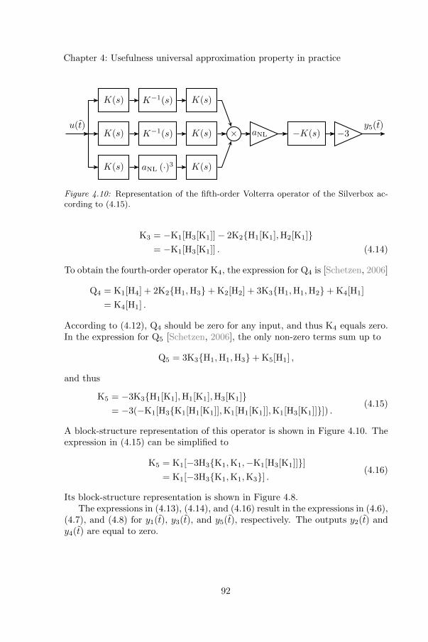
Chapter 4: Usefulness universal approximation property in practice
K(s)
K(s)
K(s)
K−1(s)
K−1(s)
aNL (·)3
K(s)
K(s)
K(s)
× aNL −K(s) −3u(t) y5(t)
Figure 4.10: Representation of the fifth-order Volterra operator of the Silverbox ac-cording to (4.15).
K3 = −K1[H3[K1]]− 2K2H1[K1],H2[K1]= −K1[H3[K1]] . (4.14)
To obtain the fourth-order operator K4, the expression for Q4 is [Schetzen, 2006]
Q4 = K1[H4] + 2K2H1,H3+ K2[H2] + 3K3H1,H1,H2+ K4[H1]
= K4[H1] .
According to (4.12), Q4 should be zero for any input, and thus K4 equals zero.In the expression for Q5 [Schetzen, 2006], the only non-zero terms sum up to
Q5 = 3K3H1,H1,H3+ K5[H1] ,
and thus
K5 = −3K3H1[K1],H1[K1],H3[K1]= −3(−K1[H3K1[H1[K1]],K1[H1[K1]],K1[H3[K1]]]) . (4.15)
A block-structure representation of this operator is shown in Figure 4.10. Theexpression in (4.15) can be simplified to
K5 = K1[−3H3K1,K1,−K1[H3[K1]]]= K1[−3H3K1,K1,K3] .
(4.16)
Its block-structure representation is shown in Figure 4.8.The expressions in (4.13), (4.14), and (4.16) result in the expressions in (4.6),
(4.7), and (4.8) for y1(t), y3(t), and y5(t), respectively. The outputs y2(t) andy4(t) are equal to zero.
92

Chapter 5
Dynamics at the output:Wiener-Hammersteinmodels
This chapter considers the identification of both single-branch and parallelWiener-Hammerstein models (see Figures 1.2c and 1.3a). After an introductionon applications, and identification and initialization methods, two initializationmethods for single-branch Wiener-Hammerstein models are proposed. Finally,a method is proposed to get rid of the cross-terms in a multivariate polynomialthat describes the static nonlinearity in a parallel Wiener-Hammerstein model.
5.1 Wiener-Hammerstein system identification
5.1.1 Applications
Since a Wiener-Hammerstein model is a generalization of both a Wiener and aHammerstein model, a Wiener-Hammerstein model can be used to model linearsystems with either sensor or actuator nonlinearities. Systems with an internalnonlinearity can be modeled as well.
Actual applications of Wiener-Hammerstein models can mainly be found inbiology [Korenberg and Hunter, 1986; Dewhirst et al., 2010; Bai et al., 2009],but also in echo cancellation [Nollett and Jones, 1997] and in the modeling ofRF power amplifiers [Isaksson et al., 2006].
93

Chapter 5: Dynamics at the output: Wiener-Hammerstein models
5.1.2 Identification methods
Several identification methods have been proposed to identify single-branchWiener-Hammerstein systems. Early work can be found in Billings and Fakhouri[1982] and Korenberg and Hunter [1986]. The maximum likelihood estimate isformulated in Chen and Fassois [1992]. Wiener-Hammerstein systems are mod-eled as the cascade of well-selected Hammerstein models in Wills and Ninness[2012]. The recursive identification of errors-in-variables Wiener-Hammersteinsystems is considered in Mu and Chen [2014].
5.1.3 Initial estimates
The identification of a Wiener-Hammerstein model is a problem that is nonlinear-in-the-parameters. Hence, good initial estimates are required. Both Chen andFassois [1992] and Wills and Ninness [2012] indicate the importance of goodinitial estimates, but not how to obtain them.
Some approaches obtain initial estimates by using specifically designed ex-periments. For example, Vandersteen et al. [1997] proposes a series of experi-ments with large and small signal multisines. Weiss et al. [1998] uses only twoexperiments with paired multisines, but the approach requires the estimation ofthe Volterra kernels of the system, which can be time-consuming. Crama andSchoukens [2005] proposes an iterative initialization scheme that only requiresone experiment of a well-designed multisine excitation.
Some other methods start from the BLA of the Wiener-Hammerstein system[Sjoberg et al., 2012; Westwick and Schoukens, 2012; Schoukens et al., 2014c].These methods are discussed in more detail below.
5.1.4 Initialization methods that start from the BLA
A major difficulty is the generation of good initial estimates for the two lineardynamic blocks. The poles and the zeros of both linear dynamic blocks can beobtained from the BLA (see Theorem 2.7). To obtain estimates for both linearblocks, the poles and the zeros of the BLA should be split over these individualblocks. Several methods have been proposed to make this split.
The brute-force method in Sjoberg et al. [2012] scans all possible splits. Foreach of these splits, the static nonlinearity is estimated via a linear least-squaresregression. The obtained initial models are then tested on the data, and thebest performing model is retained for further optimization. The drawback ofthis method is that the number of possible splits grows exponentially with themodel order. This method can thus require a large computation time.
The advanced method in Sjoberg et al. [2012] uses a basis function expansionfor the input dynamics, based on the poles of the BLA, and a basis functionexpansion for the inverse of the output dynamics, based on the zeros of the BLA.
94

5.1 Wiener-Hammerstein system identification
By expressing the static nonlinearity in terms of two multivariate polynomials,the estimation of the remaining model parameters (the polynomial coefficients)is formulated linearly-in-the-parameters. Since all the poles of the BLA areused to parameterize the input dynamics, and all the zeros of the BLA areused to parameterize the output dynamics, the model orders of the estimatedinput and output dynamics are too large. A scanning procedure over the basisfunctions is proposed to reduce these model orders. In each series of scans, allbasis functions are alternately removed. The rms error of the obtained modelsis calculated, and the best performing model is retained as an initial model.Starting from this initial model, a new series of scans is performed. Once thescanning procedure is completed, the initial models are ranked with respect totheir rms error. Typically, the rms error makes a strong jump when a necessarybasis function was removed. Compared to the brute-force method, the numberof scans is lower, but the computation time can still be large.
The method described in Westwick and Schoukens [2012] not only usesthe BLA from the input to the output, but also the so-called quadratic BLA(QBLA), which is the BLA from the squared input u2(t) to the output residualyS(t) = y(t)−GBLA(q)u(t). This QBLA is shown to be asymptotically propor-tional to the product of the output dynamics and the convolution of the inputdynamics with itself, i.e. GQBLA(k) = cQBLA[R ∗R](k)S(k) +O(N−1). Theinitialization approach in Westwick and Schoukens [2012] compares for each pos-sible split a cost function that is equal to the sum over the excited frequencies ofthe weighted differences between the QBLA obtained from the data (GQBLA(k))
and the QBLA obtained from splitting the BLA ([R[i] ∗ R[i]
](k)S[i](k) for the
ith split), where the inverse of the sample variance of GQBLA(k) is used as aweighting. A variance expression is derived for the difference between the costfunctions of two different splits, so that splits that have a significantly worsecost function than the best split can be removed from consideration. It is shownthat the number of possible splits can be greatly reduced in this way. Due tothe high-order nature of the QBLA (the ratio of the number of systematic con-tributions to the number of stochastic contributions is much smaller in a QBLAthan in a BLA), however, long measurement times may be needed to obtain anaccurate estimate.
The nonparametric separation method proposed in Schoukens et al. [2014c]avoids the pole/zero assignment problem completely, but also uses the QBLA.
This chapter proposes two initialization methods. Section 5.2 proposes ascanning procedure where the number of scans is proportional to the modelorder. Section 5.3 proposes a method based on a well-designed multisine exci-tation and a first-order BLA, where the poles and the zeros of the input dy-namics shift, while those of the output dynamics remain invariant. This makesit possible to split the poles and the zeros of the BLA over the input and the
95

Chapter 5: Dynamics at the output: Wiener-Hammerstein models
output dynamics.
5.1.5 Parallel Wiener-Hammerstein systems
Only a few identification methods for parallel Wiener-Hammerstein systemscan be found in the literature. Nevertheless, it is useful to have identificationmethods for this model structure, since parallel Wiener-Hammerstein modelsare universal approximators (see Subsection 2.2.4).
The methods proposed in Baumgartner and Rugh [1975], Wysocki andRugh [1976], and Billings and Fakhouri [1982] directly identify a decoupled(i.e. with univariate nonlinearities) parallel Wiener-Hammerstein model as inFigure 1.3a. However, they consider a somewhat restricted class of parallelWiener-Hammerstein models, called the class SM . This model has M parallelbranches, each containing a simple Wiener-Hammerstein model with an integerpower nonlinearity, i.e. branch d contains a nonlinearity (·)d. The restriction isthat there is only one branch for each power.
Up to our knowledge, only one identification method is available for a gen-eral parallel Wiener-Hammerstein model [Schoukens et al., 2015b]. It representsthe static nonlinear block by a basis function expansion (e.g. multivariate poly-nomial basis functions, piece-wise linear basis functions, or radial basis functionnetworks with a fixed width and a fixed center). If a multivariate polynomialbasis is chosen, then this polynomial typically contains cross-terms (a coupledpolynomial representation).
Section 5.4 presents a tensor decomposition method to get rid of the cross-terms in the multivariate polynomial. This makes the model easier to interpretand a possible reduction of the number of parameters is realized.
5.2 Initial estimates using basis function expan-sions
Based on Tiels et al. [2014a].
This section presents a method to initialize the three sub-blocks in a single-branch Wiener-Hammerstein model. The three sub-blocks are parameterizedin terms of basis function expansions. To reduce the number of parameters, asimplified scanning procedure is proposed.
5.2.1 Setup
The data-generating system is assumed to be a single-branch discrete-timeWiener-Hammerstein system (see Figure 5.1). Note that the representation inFigure 5.1 is not unique. Arbitrary non-zero scaling factors can be exchanged
96

5.2 Initial estimates using basis function expansions
R(q) f(x) S(q)u(t) x(t) w(t) y(t)
Figure 5.1: The data-generating system is a discrete-time Wiener-Hammerstein sys-tem (R(q) and S(q) are discrete-time linear dynamic systems, f(x) is a static nonlinearfunction).
between the linear dynamics and the static nonlinearity without changing theinput/output behavior of the system (see Figure 5.2). Also a delay can beexchanged between the two linear dynamic sub-blocks.
The following assumptions are made on the system and the signals.
Assumption 5.1 (Proper, finite-dimensional, stable, rational transfer functionsof known order). The linear dynamic systems R(q) and S(q) are proper, finite-dimensional, stable, rational transfer functions of known order.
Assumption 5.2 (No pole-zero cancellations). There are no pole-zero cancel-lations in the product R(q)S(q).
Assumption 5.3 (Non-even nonlinearity). The function f(x) is non-even aroundthe operating point.
Assumption 5.4 (Gaussian excitation). The excitation signal is either a Gaus-sian noise (see Definition 2.1) or a random-phase multisine (see Definition 2.3).
The same noise assumption is made as in Assumption 3.6, which is repeatedhere for convenience of the reader.
Assumption 5.5 (Zero-mean filtered white output noise). The measurementnoise v(t) is obtained by filtering a sequence of independent random variables,that are independent of the excitation signal u(t) and that have a zero mean anda bounded variance, by a stable monic filter.
Under this assumption, the classical least-squares framework is known toresult in consistent estimates of the BLA [Pintelon and Schoukens, 2012]. Tosimplify the notation, and without loss of generality, the results in this sectionare presented in the noise-free case.
5.2.2 Basic idea
The basic idea is to parameterize both the input and the output dynamicsin terms of GOBFs that are constructed based on all the poles of the BLA,and to parameterize the static nonlinearity by a multivariate polynomial. Theobtained model is thus the cascade of a Wiener-Schetzen model and a linear
97

Chapter 5: Dynamics at the output: Wiener-Hammerstein models
ceq1R(q)q−τ 1
ceq2f(
xceq1
)ceq2
S(q)qτu(t) ceq1
x(t− τ) 1ceq2
w(t− τ) y(t)
Figure 5.2: Arbitrary non-zero scaling factors ceq1 and ceq2 can be exchanged betweenthe linear dynamics and the static nonlinearity in the Wiener-Hammerstein system inFigure 5.1, without changing the input/output behavior of the system. Moreover, anarbitrary delay τ can be exchanged between the two linear dynamic sub-blocks.
dynamic model. A scanning procedure is proposed to reduce the number ofpoles in both sets of GOBFs. Next, the Wiener-Schetzen model is projected toa single-branch Wiener system in order to obtain initial estimates for the threesub-blocks of the Wiener-Hammerstein system. This approach is explained inmore detail in the next subsection.
5.2.3 Proposed method
A model bilinear in its parameters
The input and output dynamics R and S, and the static nonlinearity f areparameterized in terms of basis function expansions:
R(q) =
nα∑
i=0
αR,iFi(q) , (5.1)
f(x) =
D∑
d=0
γdxd , (5.2)
S(q) =
nα∑
i=0
αS,iFi(q) , (5.3)
where F0(q) = 1 is a feed-through term, and where F1(q), . . . , Fnα(q) areGOBFs that are constructed based on all the poles of the BLA of the Wiener-Hammerstein system. For simplicity reasons, we assume that there is no delayin both R(q) and S(q), although this situation can be easily dealt with. Alsofor simplicity reasons, the basis function expansion of the static nonlinearity ishere assumed polynomial. The Wiener part described by (5.1) and (5.2) canthen be rewritten as a Wiener-Schetzen model (see Section 3.3). This results in
98

5.2 Initial estimates using basis function expansions
F0(q)
Fnα(q)
β1
βnβ
+
F0(q)
Fnα(q)
α0
αnα
+ +u(t)
x0(t)
xnα(t)
w1(t)
wnβ (t)
w(t)
yDC
y(t)...
......
... f(x
0,...,xnα)
Figure 5.3: The resulting intermediate model is the cascade of a Wiener-Schetzenmodel and a linear dynamic model (F0(q), . . . , Fnα(q) are OBFs based on the poles
of the BLA;f(x0, . . . , xnα) is a MIMO polynomial).
the model structure shown in Figure 5.3 that is described by
xi(t) = Fi(q)u(t) , for i = 0, . . . , nα ,
wi(t) =f [i](x0(t), . . . , xnα(t)), for i = 1, . . . , nβ ,
w(t) =
nβ∑
i=1
βiwi(t) ,
y(t) =
nα∑
i=0
αiFi(q)w(t) + yDC ,
(5.4)
where everyf [i](x0, . . . , xnα) is a monomial of the multivariate polynomial
f(x0, . . . , xnα) with corresponding coefficient βi, and where we have droppedthe subscript S from αS,i to simplify the notation. The constant term that
corresponds to γ0 in (5.2) is not included inf , but it is estimated at the out-
put of the model (yDC in Figure 5.3). Since nβ corresponds to the number ofpolynomial coefficients in a multivariate polynomial, nβ can become quite large(see also Table 1.1).
Note that this intermediate model is bilinear in its model parameters αand β. General purpose methods to solve problems that are bilinear in theirparameters, like the methods in Bai and Liu [2005], can thus be applied.
Note also that a Wiener system (the setting of Section 4.1) and a Ham-merstein system (the setting of Section 4.2) fit in the general model structurein Figure 5.3. If there are no output dynamics (Wiener) or no input dynam-ics (Hammerstein), then the model in Figure 5.3 reduces to a model that islinear-in-the-parameters.
Over-parameterization method
Under Assumption 5.1 and in case the static nonlinearity is a polynomial, theintermediate model can exactly reproduce the input/output behavior of the true
99

Chapter 5: Dynamics at the output: Wiener-Hammerstein models
system. The output spectrum at frequency k (not including DC) is then givenby
Y (k) = S(k)W (k)
=[F0(k) · · ·Fnα(k)
]α0
...αnα
[β1 · · ·βnβ
]W1(k)
...Wnβ (k)
= F (k)θW T (k) .
(5.5)
Applying the “vec” operation on the last equation results in
vec(Y (k)) = Y (k)
= (W (k)⊗ F (k)) vec(θ)
= J(k) vec(θ) .
(5.6)
Note that J(k) is a row vector. Collecting (5.6) at all measured frequencies kresults in
Y = J vec(θ) . (5.7)
In a first step, vec(θ) is estimated via a linear least-squares approach. Next,the singular value decomposition (SVD) of the obtained parameter matrix θLS
in (5.5) is taken, and is truncated to the first term to obtain estimates for theα and β coefficients. This corresponds to the over-parameterization approachin Bai and Liu [2005].
From numerical simulations, we have observed that the regression matrix
J ∈ CN×(nα+1)nβ has rank n1nα + nβ , where n1 = nβ − (nα+D)!nα!D! + 1. The ma-
trix J is thus rank-deficient as soon as nα > 0. Hence, the over-parameterizationmethod is not convergent in this case, as the first step does not converge to thetrue θ = αβT . Let vec(θ[i]) be in the null space of J . Then θLS is just one of
the infinitely many solutions θall = θLS +∑corank(J)i=1 κiθ
[i] to the least-squaresproblem in (5.7). To find the true θ, one would need to find the κis such that θall
is of minimal rank. This problem is known as the MinRank problem [Faugereet al., 2008], which is hard to solve. Nevertheless, the over-parameterizationmethod can be used to calculate the modeled output using (5.7), and to obtainstarting values for the α and β coefficients.
Simplified scanning procedure
It should be noted that the model in (5.4) is too complex, since both the pa-rameterizations of R and S in (5.1) and (5.3) use the pole estimates of bothR and S. To reduce the complexity of the model, the user can decide to starta simplified scanning procedure. The rms error of the full-complexity model,
100

5.2 Initial estimates using basis function expansions
calculated using (5.7), will serve as a reference level with which the results ofthe scanning procedure will be compared.
In each scan, one pole (or complex conjugate pole pair for complex poles) isalternately removed from R and S in (5.1) and (5.3), respectively. The least-squares estimate in (5.7) is calculated for both reduced-complexity models. Ifthe rms error on the simulated output strongly deteriorates with respect to thereference level of the full-complexity model if a pole (or pole pair) is removedfrom, say, the input dynamics, while the rms error does not deteriorate muchwhen the pole (pair) is removed from the output dynamics, then this pole (pair)is removed from the output dynamics in the final model and is kept in theinput dynamics in the final model, and vice versa. After scanning, the over-parameterization method is applied to the final model to obtain initial estimatesfor the α and β coefficients.
This scanning procedure requires at most 2nα scans. Compared to the scan-ning procedures presented in Sjoberg et al. [2012], where the number of scansgrows either exponentially (if no restrictions on properness of the subsystems,etc. are imposed) or combinatorially with the model order, the proposed sim-plified scanning procedure requires a number of scans that is only proportionalto the model order.
Bilinear optimization
Next, the estimates of the α and β coefficients are optimized using a normal-ized iterative least-squares approach [Bai and Liu, 2005]. In each iteration,either the α or β coefficients are estimated, while the other set of coefficientsremains constant. The norm of β is normalized to one in each iteration, andthe first non-zero element of β is constrained to be positive to obtain a uniqueparameterization.
After this step, an estimate of S(q) in (5.3) is available. To obtain estimatesof R(q) and f(x), we need to project the Wiener-Schetzen model between u(t)and w(t) to a single-branch Wiener system.
Returning to a single-branch model
First, the intermediate signals xi(t) and w(t) in (5.4) are simulated using themeasured input signal u(t) and the estimated model. The simulated interme-diate signal w(t) is an estimate of w(t) in the Wiener-Hammerstein systemshown in Figure 5.1. The BLA from u(t) to w(t) is equal to R(q), up to anunknown scaling factor (special case of Theorem 2.7) that can be exchangedwith the static nonlinearity (see Figure 5.2). An estimate of (a scaled versionof) R(q) can thus be obtained by estimating the BLA from u(t) to w(t). Thenonparametric and parametric estimation of this BLA are combined in one step
101

Chapter 5: Dynamics at the output: Wiener-Hammerstein models
as
αR = arg minαR
∥∥∥∥∥w(t)−nα∑
i=0
αR,ixi(t)
∥∥∥∥∥
2
2
,
where the parameterization in (5.1) is used for the parametric estimation of theBLA.
Approximate pole-zero cancellations in the estimates of R(q) and S(q) areremoved.
Next, the polynomial coefficients γd in (5.2) are estimated using a linearleast-squares approach.
Finally, the parameters of the single-branch Wiener-Hammerstein model (itspolynomial and transfer function coefficients) can be further optimized using aLevenberg-Marquardt nonlinear optimization algorithm [Marquardt, 1963].
5.2.4 Illustration
This subsection illustrates the approach on a simulation example. The situationwhere the simplified scanning procedure is not included is compared to thesituation where it is included.
Setup
Consider the Wiener-Hammerstein system in Figure 5.1. The linear dynamicsR(q) and S(q) are second-order low-pass Chebyshev Type I filters with a peak-to-peak ripple of 10 dB and 20 dB, respectively, and with a normalized passbandedge frequency of 0.05 and 0.1, respectively. The static nonlinearity is given byf(x) = atan(2x).
The excitation signal u(t) is a random-phase multisine containing N = 1024samples. The excited frequencies are equidistantly spaced between DC and onesixth of the sample frequency, which is normalized to fs = 1 Hz. Within thisrange, the amplitudes |Uk| are chosen equal to each other and such that therms value of u(t) is equal to one. Seven phase realizations and three periods ofthe multisine are applied. The first period is removed to avoid the influence ofthe transients. A zero-mean white Gaussian disturbance v(t) is added to theoutput, with a signal-to-noise ratio of 60 dB.
Simplified scanning not included
The BLA of the system is estimated by averaging out the division of the outputand the input spectrum over the seven phase realizations. On top of this non-parametric estimate, a fourth-order parametric model is estimated. The polesof this parametric model are used to construct two sets of GOBFs, one for theinput dynamics and one for the output dynamics. The nonlinearity is modeled
102

5.2 Initial estimates using basis function expansions
0 0.05 0.1 0.15−40
−30
−20
−10
0
Frequency (in Hz)
Am
pli
tud
e(i
nd
B)
Figure 5.4: The true (full line) and estimated (dashed line) input (red) and output(blue) dynamics agree well when the scanning procedure is not included.
using a low-degree (D = 3) MIMO polynomialf to limit the number of β pa-
rameters. Starting values for the α and β coefficients are obtained using theover-parameterization method. These coefficients are then bilinearly optimized.
Initial estimates for R(q) and f(x) are obtained by projecting the Wiener-Schetzen model to a single-branch Wiener system, as described in Subsec-tion 5.2.3. In this step, the static nonlinearity is estimated with a higher-degreepolynomial (D = 5), as the number of polynomial coefficients γd only increasesproportionally with the degree as opposed to the combinatorial increase for theMIMO polynomial coefficients βi.
Figure 5.4 shows the true and the estimated linear dynamics, while Fig-ure 5.5 shows the true and the estimated static nonlinearity. The estimates arenormalized, such that the estimated linear dynamic system R and the estimatedstatic nonlinearity f match their true counterparts as well as possible in mean-square sense. The remaining normalization factor is taken into account in theestimate of S (see Figure 5.2). It can be observed that the estimates agree wellwith the true dynamics and nonlinearity.
Simplified scanning included
To see the effect of the simplified scanning procedure, the model estimationis repeated. this time including the scanning procedure described in Subsec-tion 5.2.3.
103

Chapter 5: Dynamics at the output: Wiener-Hammerstein models
−1.5 −1 −0.5 0 0.5 1 1.5−2
−1
0
1
2
x
f(x
)
Figure 5.5: The true (full line) and estimated (dashed line) static nonlinearity agreewell when the scanning procedure is not included.
Table 5.1 shows the results of the scanning procedure. It can be deducedthat the estimated pole pair 0.8811± 0.4275j should be assigned to the outputdynamics, while the pole pair 0.9404± 0.2163j should be assigned to the inputdynamics. This is in good agreement with the true dynamics. Whereas R(q)has a complex pole pair 0.9397± 0.2162j, S(q) has a pole pair 0.8800± 0.4275j.
Figures 5.6 and 5.7 show the true and estimated linear dynamics and nonlin-earity, respectively. Again, good initial estimates are obtained, but they are notas good as when the scanning procedure was not applied. Figure 5.6 only showsamplitude information, but a phase error in the estimate of S(q) is present aswell. Note that due to the scanning procedure, less correction terms are present,which causes the deterioration. Although the initial estimates are not as good,the scanning procedure allowed us to reduce the complexity of the model beforethe bilinear optimization. Moreover, both initial estimates converge to simi-lar estimates after a Levenberg-Marquardt optimization [Marquardt, 1963] (seeFigures 5.8 and 5.9).
5.2.5 Conclusion
Initial estimates for a Wiener-Hammerstein model can be obtained by usingbasis function expansions for the three sub-blocks. By parameterizing the dy-namics in terms of GOBFs that are constructed based on the poles of the BLA,and the nonlinearity in terms of a polynomial, the Wiener-Hammerstein model
104

5.2 Initial estimates using basis function expansions
0 0.05 0.1 0.15−40
−30
−20
−10
0
Frequency (in Hz)
Am
pli
tud
e(i
nd
B)
Figure 5.6: The true (full line) and estimated (dashed line) input (red) and output(blue) dynamics also agree well when the scanning procedure is included.
−1.5 −1 −0.5 0 0.5 1 1.5−2
−1
0
1
2
x
f(x
)
Figure 5.7: The true (full line) and estimated (dashed line) static nonlinearity alsoagree well when the scanning procedure is included.
105

Chapter 5: Dynamics at the output: Wiener-Hammerstein models
0 0.05 0.1 0.15−40
−30
−20
−10
0
Frequency (in Hz)
Am
pli
tud
e(i
nd
B)
Figure 5.8: The optimized estimates with (dotted line) and without (dashed line)inclusion of the scanning procedure are similar to each other and agree well with thetrue (full line) input (red) and output (blue) dynamics.
−1.5 −1 −0.5 0 0.5 1 1.5−2
−1
0
1
2
x
f(x
)
Figure 5.9: The optimized estimates with (dotted line) and without (dashed line)inclusion of the scanning procedure are similar to each other and agree well with thetrue (full line) static nonlinearity.
106

5.3 Initial estimates using phase-coupled multisines
Table 5.1: Relative rms error on the simulated output in dB when a complex conjugatepole pair is removed from the full-complexity model. The relative rms error of thefull-complexity model is equal to −24.9 dB.
Pole estimates Removed from
input dynamics output dynamics
0.8811± 0.4275j −24.4 dB −14.9 dB0.9404± 0.2163j −13.7 dB −24.8 dB
is reformulated to the cascade of a Wiener-Schetzen model and a linear dynamicmodel. This intermediate model is bilinear in its parameters. A simplified scan-ning procedure can be performed to reduce the number of poles used in each setof GOBFs. After a bilinear optimization of the model parameters, the Wiener-Schetzen part of the intermediate model is projected to a single-branch Wienermodel. This results in an initial estimate of the Wiener-Hammerstein system.
The method, as presented here, still has problems to converge for high-orderWiener-Hammerstein systems. If the linear dynamics are high-order, it is notalways clear for each pole (pair) whether it should be assigned to the input orto the output dynamics. This is likely due to the fact that the large numberof poles compensate for the pole mismatch when a necessary pole is removed.Moreover, the intermediate model has a large number of parameters when thedynamics are high-order. Hence, the variance error may become quite large.The scanning procedure could however be simplified. Compared to the expo-nential or combinatorial increase of the number of scans with the model orderin related scanning methods, the number of scans increases only proportionallywith the model order in the proposed simplified scanning procedure.
5.3 Initial estimates using phase-coupled multi-sines
Based on Tiels et al. [2014b].
This section presents an alternative method to initialize the linear dynamicblocks in a single-branch Wiener-Hammerstein model. A well-designed multi-sine excitation is used to split the overall dynamics of the BLA over the inputand the output dynamics.
5.3.1 Setup
The setup is slightly different than the one in Subsection 5.2.1.
107

Chapter 5: Dynamics at the output: Wiener-Hammerstein models
This time, it should only be possible to approximate the nonlinearity by a(possibly infinite-degree) polynomial. The nonlinearity itself will not be esti-mated. Note that a uniformly convergent polynomial approximation is alwayspossible for a continuous nonlinearity on a closed interval due to the Stone-Weierstrass theorem. The type of convergence can even be relaxed to mean-square convergence, since the BLAs that will be estimated make use of mean-square approximation. Hence, discontinuous nonlinearities are also allowed.
Assumption 5.6 (Polynomial nonlinearity representation). The static nonlin-earity f(x) can be arbitrarily well approximated by a polynomial in the interval[min(x(t)),max(x(t))]. Hence, f(x) can be thought of as f(x) =
∑∞d=0 γdx
d.
An assumption that is slightly stricter than the non-evenness of the nonlin-earity is required.
Assumption 5.7 (Nonlinear odd term present). At least one nonlinear oddterm is present, i.e. there exists an odd d ≥ 3 for which γd 6= 0.
Moreover, transients are not considered here.Finally, Assumption 5.5 is made as well. To simplify the notation, and
without loss of generality, also the results in this section are presented in thenoise-free case.
Assumption 5.8 (Noise-free). The input and output are measured withoutdisturbing noise.
5.3.2 Basic idea
The BLA of a Wiener-Hammerstein system for a Gaussian excitation is propor-tional to the product of the underlying linear dynamic blocks (see Theorem 2.7).The basic idea here is to introduce a multisine excitation with pairwise coupledrandom phases. Compared to the random-phase multisine case explained inAppendix 2.A, new terms will pop up in the output spectrum. A modified BLAwill be estimated on a shifted frequency grid. It will be shown that the inputdynamics shift over a user-specified frequency offset in this shifted BLA, whilethe output dynamics remain fixed. This allows us to separate the overall dy-namics obtained from the BLA over the input and the output dynamics. Theapproach is explained in more detail below.
5.3.3 Phase-coupled multisine excitation
Phase-coupled multisines are multisines where specifically selected pairs of ex-cited harmonics have the same phase. Depending on whether both even andodd, or only odd harmonics are excited, we are dealing with a full or an oddphase-coupled multisine, respectively.
108

5.3 Initial estimates using phase-coupled multisines
Definition 5.9 (Full phase-coupled multisine). A signal u(t) is a phase-coupledmultisine if it is a multisine (see Definition 2.2) that only excites the harmonicsk for which
±k ∈(
ζ
2+ ζi,
ζ
2+ ζi+ s
)for i = 0, 1, . . . , imax ,
where ζ and s are integers (more details below), and if each of the frequencycouples gets assigned an independently and identically distributed random phase
φ ζ2 +ζi = φ ζ
2 +ζi+s with the property Eejφ ζ
2+ζi
= 0. For a full phase-coupled
multisine, the even integer ζ ≥ 4 determines the frequency resolution (only ev-ery ζth harmonic is excited, starting from the harmonics ζ
2 and ζ2 + s), and
s = cshiftζ + 1 will determine the shift of the poles and the zeros of R(q) withrespect to those of S(q), where cshift > 0 is an integer.
It can be useful to only excite the odd harmonics, just as with random-phase multisines [Schoukens et al., 2005]. The definition of the phase-coupledmultisine then slightly changes.
Definition 5.10 (Odd phase-coupled multisine). A signal u(t) is an odd phase-coupled multisine if it is a phase-coupled multisine (see Definition 5.9) whereζ2 ≥ 5 is an odd integer, and where s = cshiftζ + 2.
To simplify the notation hereafter, define
ν :=ζ
2+ ζi . (5.8)
Note that there is some abuse of notation, since the dependency on i is nottaken into account in the notation ν.
Remark 5.11. Although this is not really necessary, the requirement ζ ≥ 4for a full phase-coupled multisine, and ζ
2 ≥ 5 for an odd phase-coupled multi-sine makes sure that the harmonics k = ν − s and k = ν + 2s are not excited.Hence, the output spectrum at these harmonics will not be disturbed by linearcontributions.
5.3.4 New terms in the output spectrum of the BLA
Consider the setting in Appendix 2.A, where the random-phase multisine caseis explained. Since U(ν) and U(ν + s) have the same phase in a phase-coupledmultisine, also other terms than the ones reported in (2.20) will contribute tothe BLA at the harmonics ν and ν+s when a phase-coupled multisine excitationis used. Moreover, the output spectrum will contain terms that are proportional
109

Chapter 5: Dynamics at the output: Wiener-Hammerstein models
to S(k) and shifted versions of R(k) at some non-excited harmonics. This isexplained below.
Let us take a look at the terms in Yd(k) in (2.19) where the product∏di=1 U(li)
has a phase ∠U(ν). These are the terms where one of the harmonics li is equalto ν or ν + s (U(ν + s) has the same phase as U(ν)), and where the remaining
factors in the product∏di=1R(li)U(li) combine pairwise to a constant. The
possible values for these d−12 (complex) constants are either
c0 =
N/2∑
l=−N/2+1
X(l)X(−l) ,
c−s =
N/2∑
l=−N/2+1
X(l)X(−(l + s)) ,
or
cs =
N/2∑
l=−N/2+1
X(−l)X(l + s) .
Note that whenever a pair of factors combines to c−s, a frequency shift −sis introduced in the sum
∑di=1 li = k. Likewise, a frequency shift s is intro-
duced whenever a pair of factors combines to cs = (c−s)∗. There are thus d+ 1
harmonics k that range from ν − d−12 s to ν + d+1
2 s in steps of s where the prod-
uct∏di=1 U(li) has a phase ∠U(ν). The smallest harmonic (k = ν − d−1
2 s) isobtained when one of the harmonics li is equal to ν, and when all the otherharmonics form pairs (l,−(l + s)). The largest harmonic (k = ν + d+1
2 s) is ob-tained when one harmonic li is equal to ν + s, and when all the other harmonicsform pairs (−l, l + s). From the discussion above, the following theorem follows:
Theorem 5.12. For the Wiener-Hammerstein system in Figure 5.1, excited bya phase-coupled multisine (see Definitions 5.9 and 5.10), operating in steady-
state, and under Assumptions 5.6 and 5.8, the expectation Eu
Yd(ν+is)U(ν)
is
equal to
d!S(ν + is)
R(ν)
∑
sk∈Sd−12
is
d−12∏
k=1
csk
+ R(ν + s)|U(ν + s)||U(ν)|
∑
sk∈Sd−12
(i−1)s
d−12∏
k=1
csk
+O(N−1) ,
110

5.3 Initial estimates using phase-coupled multisines
and the expectation Eu
Yd(−(ν+is))
U(−ν)
=(Eu
Yd(ν+is)U(ν)
)∗is equal to
d!S(−(ν + is))
R(−ν)
∑
sk∈Sd−12−is
d−12∏
k=1
csk
+ R(−(ν + s))|U(ν + s)||U(ν)|
∑
sk∈Sd−12−(i−1)s
d−12∏
k=1
csk
+O(N−1)
(5.9)
for i = −d−12 ,−d−1
2 + 1, . . . , d+12 , and where the set Sdl is defined as
Sdl := sk : sk ∈ −s, 0, s ∧d∑
k=1
sk = l .
Proof. The theorem follows immediately from the discussion above.
Note that Eu
Yd(ν+is)U(ν)
and Eu
Yd(−(ν+is))
U(−ν)
are zero if Assumption 5.7
is not fulfilled.From here on, the error term O(N−1) will be dropped.
For example, for d = 3, there are four harmonics where Eu
Y3(k)U(ν)
has a
non-zero mean. These are listed below.
• At harmonic k = ν − s:
Eu
Y3(k)
U(ν)
= 6S(ν − s)R(ν)c−s
• At harmonic k = ν:
Eu
Y3(k)
U(ν)
= 6S(ν)R(ν)c0
+ 6S(ν)R(ν + s)|U(ν + s)||U(ν)| c−s
• At harmonic k = ν + s:
Eu
Y3(k)
U(ν)
= 6S(ν + s)R(ν)cs
+ 6S(ν + s)R(ν + s)|U(ν + s)||U(ν)| c0
111

Chapter 5: Dynamics at the output: Wiener-Hammerstein models
• At harmonic k = ν + 2s:
Eu
Y3(k)
U(ν)
= 6S(ν + 2s)R(ν + s)
|U(ν + s)||U(ν)| cs
The results at the harmonics k = ν − s and k = ν + 2s are of particular in-
terest. At these harmonics, Eu
Y3(k)U(ν)
is proportional to S(k)R(k + s) and
S(k)R(k − s), respectively. The frequency shift of the input dynamics R overa frequency −s (or s) creates a shift of the poles and the zeros of R over afrequency −s (or s). Note that the shifted poles and zeros are no longer realnor paired in complex conjugated couples. Hence, the rational transfer func-
tions related to Eu
Y3(ν−s)U(ν)
and Eu
Y3(ν+2s)U(ν)
will have complex coefficients
instead of real coefficients. This will be used in the next subsection.
5.3.5 The shifted BLA and parametric smoothing
For simplicity, we continue to explain the idea on a third-degree nonlinearity.The generalization to an arbitrary degree d is explained in Subsection 5.3.6.
First, the FRF measurements Eu
Y3(k)U(ν)
and Eu
Y3(k)U(−ν)
will be collected at
appropriate harmonics k, such that only contributions are selected where theinput and output dynamics shift over a unique frequency offset. Next, a para-metric transfer function model will be identified to get direct access to the polesand the zeros of the system. As the shifted poles result in a transfer func-tion model with complex coefficients, an adapted frequency domain estimator[Peeters et al., 2001] will be used. Finally, the input and the output dynamicswill be split by separating the shifting poles and zeros from those that do notmove.
From (5.9), it follows that
Eu
Y3(−(ν − s))
U(−ν)
= 6S(−(ν − s))R(−ν)cs
and that
Eu
Y3(−(ν + 2s))
U(−ν)
= 6S(−(ν + 2s))R(−(ν + s))
|U(ν + s)||U(ν)| c−s .
Consequently, Eu
Y3(k)U(−ν)
is proportional to S(k)R(k − s) at the harmon-
ics k = −(ν − s), while it is proportional to S(k)R(k + s) at the harmonicsk = −(ν + 2s). Therefore, by analogy with (2.9), define the shifted BLAs
G+SBLA(k) and G−SBLA(k) by collecting Eu
Y (k)U(ν)
and Eu
Y (k)U(−ν)
at the ap-
propriate harmonics k, such that contributions proportional to S(k)R(k + s)and S(k)R(k − s), respectively, result:
112

5.3 Initial estimates using phase-coupled multisines
Definition 5.13 (Shifted best linear approximation). For a system excitedby a phase-coupled multisine (see Definitions 5.9 and 5.10), the shifted BLAG+
SBLA(k) is defined as
G+SBLA(k) :=
Eu
Y (k)U(ν)
at k = ν − s
Eu
Y (k)U(−ν)
at k = −(ν + 2s)
while the shifted BLA G−SBLA(k) is defined as
G−SBLA(k) :=
Eu
Y (k)U(ν)
at k = ν + 2s
Eu
Y (k)U(−ν)
at k = −(ν − s)
(5.10)
with ν defined in (5.8).
Since G−SBLA(k) = (G+SBLA(−k))
∗, we can focus completely on one of both,
e.g. G−SBLA(k).Since phase-coupled multisines rely on the fact that some harmonics have
equal phase, the time origin is important when estimating the shifted BLAfrom measured input/output data. This synchronization issue is addressed inAppendix 5.A.
Next, a parametric transfer function model is identified on G−SBLA(k), usinga weighted least-squares estimator [Peeters et al., 2001]
θ = arg minθ
K(θ) , (5.11a)
where the cost function K(θ) is equal to
1
N
∑
k∈ν+2s,−(ν−s)
|G−SBLA(k)−G−SBLA(k,θ)|2σ2G−SBLA
(k). (5.11b)
Here, σ2G−SBLA
(k) is the sample variance of G−SBLA(k), and G−SBLA(k,θ) is a para-
metric transfer function model:
G−SBLA(k,θ) =
∑nbR+nbSl=0 bSBLA,le
−j2π kN l
∑naR+naSl=0 aSBLA,le−j2π
kN l
,
with the complex coefficients bSBLA,l and aSBLA,l collected in the parametervector θ. Since G−SBLA(k) is proportional to S(k)R(k − s), the poles (and thezeros) of R will be shifted over a frequency offset s, and will no longer be real, norcomplex conjugated. By comparing the poles (and the zeros) of G−SBLA(k,θ)and their complex conjugates, the poles (and the zeros) of R and S can be
separated. Indeed, a frequency shift ej2π2sN will be visible in the complex plane
between the shifted poles (and zeros) of R and their complex conjugates, whilethe poles (and zeros) of S will not show this shift. Figure 5.10 shows an exampleof the pole shifting.
113

Chapter 5: Dynamics at the output: Wiener-Hammerstein models
−1 0 1−1
−0.5
0
0.5
1
φ
Real part
Imag
inar
yp
art
Figure 5.10: Original poles (black) of the input dynamics shift in the shifted BLA.Hence, the shifted poles (red) and their complex conjugates (blue) show a frequencyshift in the complex plane (φ = 2π 2s
N).
5.3.6 Generalization to arbitrary degree polynomial non-linearities
The basic idea, that was explained for a cubic nonlinearity in the previoussubsection, is now generalized to an arbitrary degree d. Under Assumption 5.7,the result in Theorem 5.12 can be used to separate the input and the outputdynamics. The main concern, however, is that the shifted BLAs will containcontributions where the input and the output dynamics are shifted over distinctfrequencies if d ≥ 5. This will be addressed now.
The results in Theorem 5.12 show that the shifted BLA G−SBLA(k) will notonly contain terms that are proportional to S(k)R(k − s) for d ≥ 5, but alsoterms that are proportional to S(k)R(k − 2s). One way to deal with thisis to redefine the shifted BLA, thereby only considering the outer harmon-ics k = ν − D−1
2 s and k = ν + D+12 s, where a unique frequency shift of R is
present. The main disadvantage of this approach is that it requires knowledgeof the maximal degree of nonlinearity D. Moreover, in order not to be dis-turbed by linear contributions at these harmonics, the frequency resolution ofthe phase-coupled multisine excitation should be lowered (cfr. Remark 5.11).Therefore, a different approach is followed here.
Both the contributions proportional to S(k)R(k − s) and S(k)R(k − 2s) will
114

5.3 Initial estimates using phase-coupled multisines
make the poles of R shift over a positive frequency offset, while those of S willremain fixed. Hence, the poles and the zeros of R and S can still be sepa-rated. Since two distinct frequency shifts of the input dynamics are presentin the shifted BLA, its parametric model should have a larger model order,namely the model order of S plus two times the model order of R. Thiswill not be done, however, because the contributions that are proportional toS(k)R(k − s) are dominant over those that are proportional to S(k)R(k − 2s)(see Appendix 5.B), certainly if we assume that the cubic nonlinearities domi-nate the higher-order contributions. Hence, the terms in G−SBLA(k) that are notproportional to S(k)R(k − s) will simply be considered as nuisance terms.
5.3.7 Illustration
This subsection illustrates the proposed method on a simulation example and onexperimental data obtained from the Wiener-Hammerstein benchmark system[Schoukens et al., 2009b].
Simulation example
Consider a discrete-time Wiener-Hammerstein system (see Figure 5.1). The lin-ear dynamic systems R(q) and S(q) are both second-order low-pass ChebyshevType I filters with 20 dB peak-to-peak ripple in the passband. The normalizedpassband edge frequency of R(q) and S(q) is equal to 0.05 and 0.1, respectively.The static nonlinear function f(x) = 10x3 is a cubic nonlinearity.
The system is excited with one random-phase multisine and two phase-coupled multisines. These multisines contain N = 8192 samples. They have anrms value equal to one, and have a flat amplitude distribution between DC andone sixth of the sample frequency fs = 1 Hz. The random-phase multisine hasequidistantly spaced excited harmonics within this range. The phase-coupledmultisines have the following properties (see Definition 5.9): ζ = 4, s = 41, andimax = 330 for the first multisine, and ζ = 4, s = 81, and imax = 320 for thesecond multisine. One thousand phase realizations of the random-phase andphase-coupled multisines are applied to be able to show sufficiently smoothnonparametric estimates of the BLA and the shifted BLAs. In practical appli-cations, this number can be strongly reduced. Two periods of the multisinesare applied. The first period is removed to avoid the effect of transients.
From the results in Figure 5.11, it can be seen that the input dynamicsindeed shift over a user-specified frequency offset in the shifted BLA, while theoutput dynamics remain fixed. This allows us to split the overall dynamics ofthe BLA over the input and the output dynamics.
115

Chapter 5: Dynamics at the output: Wiener-Hammerstein models
0 0.05 0.1 0.15−120
−100
−80
−60
−40
−20
0
Frequency (Hz)
Am
pli
tud
e(d
B)
R
S
BLA
Shifted BLA (s = 41)
Shifted BLA (s = 81)
Figure 5.11: The BLA of a Wiener-Hammerstein system is proportional to the productof the two linear dynamic blocks for a Gaussian distributed excitation. When usinga phase-coupled multisine excitation, the input dynamics shift over a user-specifiedfrequency offset s (in frequency bins) in the shifted BLA, while the output dynamicsremain fixed.
f
|R|
f
|S|u(t) y(t)
Figure 5.12: The Wiener-Hammerstein benchmark system consists of a diode-resistornetwork sandwiched in between two third-order Chebyshev filters.
Experimental results on the Wiener-Hammerstein benchmark system
The Wiener-Hammerstein benchmark system is an electronic circuit with aWiener-Hammerstein structure, built by Gerd Vandersteen [Vandersteen, 1997].It consists of a diode-resistor network sandwiched in between two third-orderfilters (see Figure 5.12). The input filter R is a Chebyshev low-pass filter witha ripple of 0.5 dB and a cut-off frequency of 4.4 kHz. The output filter S isan inverse Chebyshev filter with a stop-band attenuation of 40 dB starting at5 kHz. It has a transmission zero in the frequency band of interest.
The benchmark data were obtained using a filtered Gaussian noise excitation[Schoukens et al., 2009b] and are therefore not used here. Instead, a random-phase multisine is used to measure the BLA, and an odd phase-coupled multisine
116

5.3 Initial estimates using phase-coupled multisines
−1.5 −1 −0.5 0 0.5 1 1.5
·104
−140
−120
−100
−80
−60
−40
−20
Frequency (Hz)
Am
pli
tud
e(d
B)
Figure 5.13: The shifted BLA (black dots) is not symmetric around the origin. Itsstandard deviation is shown in black triangles.
is used to measure the shifted BLA. For both excitations, the input and outputare measured at a sample frequency of 78 125 Hz.
The random-phase multisine contains N = 16 384 samples. It has a flatamplitude spectrum with 2097 equidistantly spaced excited frequencies thatrange from DC to 10 kHz, and has an rms level of 380 mV. This relatively smallrms level is chosen to keep the nonlinear distortion level small. Twenty phaserealizations and three periods are applied. The first period is removed to avoidthe effect of transients.
The phase-coupled multisine contains N = 16 384 samples as well, and alsohas a flat amplitude spectrum. With d = 10, s = 482, and imax = 224, there are450 excited frequencies that range from 24 Hz to 13 003 Hz. The signal is nor-malized to have a maximal amplitude of 2 V. This amplitude level correspondsmore or less to that of the Wiener-Hammerstein benchmark data. Again, threeperiods are applied where the first one is removed to avoid the effect of tran-sients. Five hundred phase realizations are applied to almost completely averageout the nonlinear distortions in the shifted BLA so that we can show a high-quality nonparametric estimate of the shifted BLA (see Figure 5.13). However,much less phase realizations can be used, since the parametric modeling stepwill also reduce the impact of the nonlinear distortions (and the noise). Forexample, ten phase realizations can be enough (see further).
The BLA is first estimated non-parametrically by applying the robust method[Schoukens et al., 2012] on the random-phase multisine data. Next, a parametric
117

Chapter 5: Dynamics at the output: Wiener-Hammerstein models
0 0.2 0.4 0.6 0.8 1
·104
−120
−100
−80
−60
−40
−20
0
Frequency (Hz)
Am
pli
tud
e(d
B)
Figure 5.14: A parametric fourth-order model (red line) can explain the non-parametric BLA (green) (the magnitude of the complex difference between the BLAs(red triangles) coincides with the estimated total distortion level (black)).
fourth-order transfer function model is estimated on top of the non-parametricBLA. The poles and the zeros of the parametric model are used as a refer-ence to compare them with those of the shifted BLA. Although a sixth-ordermodel is expected (R and S are both third-order filters), a fourth-order modelseems enough for the data at hand (see Figure 5.14). The pole pair that ismissing in the fourth-order model belongs to the input dynamics. Accordingto the properties of the input filter, the missing pole pair should be at about0.8389± 0.3182j, which corresponds to a frequency of about 4.5 kHz. When asixth-order model was estimated, the extra pole and zero pair was almost coin-ciding at 0.7335± 0.6799j, which corresponds to a frequency of about 9.3 kHz.A possibility to pick up the correct pole pair in the sixth-order model would beto use logarithmically spaced excited frequencies [Schoukens et al., 2012], suchthat less power is applied in the highest frequency range. This would, however,require a different implementation of the phase-coupled multisine than the onesdefined in Definitions 5.9 and 5.10.
The shifted BLA is estimated non-parametrically by averaging over the 500realizations of the phase-coupled multisine. The averaged value is shown to-gether with its standard deviation in Figure 5.13. Observe that there is a gapin the shifted BLA between 2.3 kHz and 4.6 kHz. The first frequency where
Eu
Y (k)U(ν)
is estimated in the shifted BLA in (5.10) is at k = ζ
2 + 2s, while the
118

5.3 Initial estimates using phase-coupled multisines
0 0.2 0.4 0.6 0.8 1−0.5
0
0.5
Real part
Imag
inar
yp
art
Figure 5.15: The poles of the shifted BLA are shown in red crosses, their complexconjugates in blue pluses, and the original poles of the BLA in black dots. One pole(where red and blue are not on top of each other) shows a clear shift and can beassigned to the input filter R. The three other poles (almost) remain invariant andcan be assigned to the output filter S. This is in good agreement with the internalstructures of the filters in Figure 5.12. Their poles are added in gray as a reference(triangles: R, squares: S).
last frequency where Eu
Y (k)U(−ν)
is estimated is at k = − ζ2 + s. Hence, there is
a gap of ζ + s. The shift s should thus not be made too large. Observe also thatthe amplitude characteristic is not symmetric around the origin. Hence, a para-metric transfer function model with complex coefficients is required. A fourth-order model is estimated using the weighted least-squares approach in (5.11).The poles of this model, together with their complex conjugates and the originalpoles of the BLA are shown in Figure 5.15. A similar picture for the zeros isshown in Figure 5.16.
One real pole can be assigned to the input filter R, since the correspondingpole of the shifted BLA shows a clear shift of about 21.7° with respect to itscomplex conjugate. This shift also nicely corresponds to the expected shift of2sN 360° = 21.2°. The other poles do (almost) not move. They can be assigned tothe output filter S. Considering the internal structures of the filters, the polesare assigned correctly. The input filter R should have a complex conjugate polepair as well, but its effect on the FRFs seems unnoticeable due to the presenceof the transmission zero in S.
The complex pair of zeros can be assigned to the output filter S, since these
119

Chapter 5: Dynamics at the output: Wiener-Hammerstein models
−1 −0.5 0 0.5 1−1
−0.5
0
0.5
1
Real part
Imag
inar
yp
art
Figure 5.16: Zeros of the shifted BLA are shown in red circles, their complex conju-gates in blue diamonds, and zeros of the BLA in black dots. One zero outside the unitcircle is not shown. The complex pair of zeros can clearly be assigned to the outputfilter S. The other zeros cannot be classified.
zeros do not shift. This pair of zeros is assigned correctly, as it corresponds tothe transmission zero in the output filter (see Figure 5.12). The real zero inFigure 5.16 cannot be clearly assigned. Although a shift of about 15° is presentbetween the corresponding zero of the shifted BLA and its complex conjugate,its amplitude is so small that a small uncertainty on the zero position cancompletely change its classification. The inability to assign most of the zeros isto be expected, since, except for the transmission zero, the true zeros are at −1,and that part of the frequency band is not excited. Therefore, the uncertaintyon these estimated zero positions is large, which prohibits their classification.
Similar results can be obtained when only ten phase realizations are usedinstead of five hundred. The 500 experiments were split in 50 groups of tenphase realizations. In 35 cases, a correct assignment of the poles and zeroscould clearly be made. In 12 of the remaining cases, the most damped realpole could have been wrongfully assigned to S, while the least damped realpole would then have been wrongfully assigned to R. The wrong assignment ofthese poles is likely to have a small impact on the further initialization of theWiener-Hammerstein model, since both real poles lie close to each other. Onlyin 3 cases, it was unclear whether both real poles should be assigned to R, toS, or one to R and one to S.
120

5.4 From coupled to decoupled polynomial representations
5.3.8 Conclusion
The BLA of a Wiener-Hammerstein system that is excited by Gaussian noiseor a random-phase multisine is proportional to the product of the underlyinglinear dynamic blocks. By applying a more specialized phase-coupled multisine,it is shown that a modified BLA expression is proportional to the product of theoutput dynamics and a frequency-shifted version of the input dynamics. On thebasis of the nonparametric measurement of this modified BLA, it is shown tobe possible to assign the identified poles and zeros to either the input or outputdynamics, provided that the poles and zeros are properly excited.
5.4 From coupled to decoupled polynomial rep-resentations
Based on Tiels and Schoukens [2013a].
This section considers parallel Wiener-Hammerstein models. The identifica-tion of these models quickly leads to a model structure with a coupled nonlin-earity, e.g. a multivariate polynomial with cross-terms. This section presents amethod to decouple quadratic, cubic, and eventually mixed-degrees MIMO poly-nomials that represent the static nonlinearity in a parallel Wiener-Hammersteinmodel. The methods are based on the CPD (canonical polyadic decomposition)tensor decomposition [Carroll and Chang, 1970; Harshman, 1970; Kolda andBader, 2009]. The CPD is also known as PARAFAC (parallel factors) [Harsh-man, 1970] or CANDECOMP (canonical decomposition) [Carroll and Chang,1970].
5.4.1 Setup
Consider the parallel Wiener-Hammerstein model in Figure 5.17, described by
xi(t) =
Ri(q)u(t) , i = 1, . . . , n
R,
wi(t) =
f [i](
x(t)) , i = 1, . . . , n
S,
y(t) =
nS∑
i=1
Si(q)
wi(t) ,
(5.12)
wherex(t) = [
x1(t), . . . ,
xn
R(t)]T , and where every
f [i](
x(t)) is a polynomial.
To keep the notation simple, the polynomialsf [i](
x(t)) are assumed to be sums
of quadratic and cubic polynomials, but the results extend to higher degrees.
121

Chapter 5: Dynamics at the output: Wiener-Hammerstein models
R1(q)
Rn
R(q)
...
f( x
1,..., xn R
) S1(q)
Sn
S(q)
... +u(t)
x1(t)
xn
R(t)
w1(t)
wn
S(t)
y1(t)
yn
S(t)
y(t)
Figure 5.17: Coupled representation of the parallel Wiener-Hammerstein model de-scribed by (5.12).
R1(q)
Rn(q)
...
f [1](x1)
f [n](xn)
...
S1(q)
Sn(q)
... +u(t)
x1(t)
xn(t)
w1(t)
wn(t)
y1(t)
yn(t)
y(t)
Figure 5.18: Decoupled representation of the parallel Wiener-Hammerstein modeldescribed by (5.13).
In general, the multivariate polynomialsf [i](
x(t)) contain cross-terms. We
want to eliminate these cross-terms, and thus come to a decoupled represen-tation of the parallel Wiener-Hammerstein model (see Figure 5.18), describedby
xi(t) = Ri(q)u(t) , i = 1, . . . , n ,
wi(t) = f [i](x(t)) , i = 1, . . . , n ,
y(t) =
n∑
i=1
Si(q)wi(t) .
(5.13)
In this case, the polynomials f [i](x(t)) are univariate instead of multivariate.The model representation is thus simplified to a sum of n parallel branches,each containing a simple Wiener-Hammerstein model.
The problem addressed here is how to retrieve a decoupled representation(5.13) of a parallel Wiener-Hammerstein model, given a cross-coupled repre-sentation (5.12). The goal is to keep the number of branches in the decoupledrepresentation small, i.e. keep n small.
122

5.4 From coupled to decoupled polynomial representations
5.4.2 Basic idea
Some methods already exist to decouple a MISO polynomial in Volterra models[Favier and Bouilloc, 2009] and in parallel Wiener models [Schoukens and Ro-lain, 2012a]. A disadvantage of the former is that it requires the measurementof the Volterra kernels of different orders, which can be time-consuming. Theapproach in Schoukens and Rolain [2012a] circumvents this problem. It achievesthe same result starting from a polynomial description of the cross-coupled non-linearity. The polynomial is first split in a sum of homogeneous polynomials.Next, the cross-terms in each homogeneous polynomial are eliminated usingtensor decomposition methods. A drawback is the introduction of new inputsignals for each degree in the polynomial.
This section considers the decoupling of a MIMO polynomial in parallelWiener-Hammerstein models. The focus is first on quadratic nonlinearities inSubsection 5.4.3. The square matrices that describe the quadratic forms aredecomposed on a common basis, built on a product of vectors. This results in asimultaneous decoupling across the outputs of the polynomial. Next, the idea isgeneralized to cubic polynomials in Subsection 5.4.4, showing that the methodextends to higher-degree polynomials. Finally, the approach is generalized topolynomials with mixed degrees of nonlinearity in Subsection 5.4.5. A simulta-neous decoupling, both across the outputs and the degrees of the polynomial, isthus considered. The basic idea is to impose more and more constraints, suchthat the total number of branches n is kept as small as possible.
5.4.3 Simultaneous decoupling of quadratic polynomials
Decompose the coefficient matrices on a common basis
First, quadratic polynomials are considered, i.e.
f [i](
x(t)) =
n R∑
i1=1
n R∑
i2=1
β[i]i1,i2
xi1(t)
xi2(t) .
The quadratic polynomial coefficients β[i]i1,i2
are collected in a symmetric ma-
trix B[i] ∈ Rn R×n R , such thatf [i](
x(t)) =
xT (t)B[i] x(t). The basic idea is to
decompose the matrices B[i] on a common basis, built on an outer product ofvectors λk:
B[i] ≈nquad∑
k=1
µ[i]k λkλ
Tk , (5.14)
where each µ[i]k is a scalar. Note that the basis vectors λk do not depend on i;
all the matrices B[i] are decomposed using the same basis.
123

Chapter 5: Dynamics at the output: Wiener-Hammerstein models
Decoupled parallel Wiener-Hammerstein model
Using the decomposition in (5.14), the outputs of the polynomialsf [i](
x(t)) can
be rewritten as
wi(t) =
xT (t)B[i] x(t)
≈nquad∑
k=1
µ[i]kxT (t)λkλ
Tkx(t)
=
nquad∑
k=1
µ[i]k (λTk
x(t))2
=
nquad∑
k=1
µ[i]k
n R∑
l=1
λl,kxl(t)
2
=
nquad∑
k=1
µ[i]k
n R∑
l=1
λl,kRl(q)u(t)
2
.
Defining the LTI systems Rk(q) as
Rk(q) :=
n R∑
l=1
λl,kRl(q)
allows us to writewi(t) as
wi(t) ≈
nquad∑
k=1
µ[i]k (Rk(q)u(t))
2
=
nquad∑
k=1
µ[i]k x
2k(t) .
The output of the parallel Wiener-Hammerstein model in Figure 5.17 is thenequal to
y(t) =
nS∑
i=1
Si(q)
wi(t)
≈nS∑
i=1
Si(q)
nquad∑
k=1
µ[i]k x
2k(t)
=
nquad∑
k=1
nS∑
i=1
µ[i]k
Si(q)x
2k(t) .
124

5.4 From coupled to decoupled polynomial representations
Defining the LTI systems Sk(q) as
Sk(q) :=
nS∑
i=1
µ[i]k
Si(q)
allows us to writey(t) as
y(t) ≈
nquad∑
k=1
Sk(q)x2k(t) .
Defining the univariate polynomials f [k](xk(t)) as
f [k](xk(t)) := x2k(t)
allows us to write
y(t) ≈
nquad∑
k=1
Sk(q)wk(t)
= y(t) ,
withwk(t) = f [k](xk(t)) .
A decoupled representation of the parallel Wiener-Hammerstein model, as in(5.13), is thus retrieved. The model has n = nquad branches.
Although an equal sign can be used in (5.14), we prefer to use an approxi-
mation sign, since the entries of the matrices B[i] can be corrupted with noise.An approximation with a far smaller number of terms then outweighs an exactrecovery of the matrices B[i].
Determine the basis vectors using the CPD
In the foregoing, it was shown that a coupled (quadratic) polynomial represen-tation in a parallel Wiener-Hammerstein model can be replaced by a decoupledrepresentation if a decomposition as in (5.14) can be made. Here, it is presentedhow such a decomposition can be calculated.
First, we stack the matrices B[i] in a partially symmetric third-order tensor
Mquad ∈ Rn R×n R×nS . Element-wise mquadi1,i2,i3
= β[i3]i1,i2
.Next, the CPD [Carroll and Chang, 1970; Harshman, 1970; Kolda and Bader,
2009] of this tensor is calculated. The CPD of a tensor approximates the tensorwith a sum of rank-one tensors, where the approximation is done as well aspossible in mean-square sense on the tensor entries. For example, a (partiallysymmetric) CPD of Mquad is given by
Mquad ≈nquad∑
k=1
λk λk µk ,
125

Chapter 5: Dynamics at the output: Wiener-Hammerstein models
where denotes the tensor product. This means that element-wise
mquadi1,i2,i3
≈nquad∑
k=1
λi1,kλi2,kµ[i3]k .
The elements of the the vectors λk and µk are calculated as the minimizers of
minλk,µk
∥∥∥∥∥Mquad −
nquad∑
k=1
λk λk µk
∥∥∥∥∥
2
F
,
where ‖·‖F denotes the Frobenius norm. The CPD of a tensor is often calculatedusing an alternating least-squares (ALS) approach [Kolda and Bader, 2009].Recently, other algorithms to calculate the CPD of a tensor were proposed inSorber et al. [2012, 2013a] that do better overall than ALS.
By stacking the matrices B[i] in one tensor Mquad, the basis vectors λkare common for each of the n
Smatrices B[i], which is not guaranteed if these
matrices are decomposed separately. To obtain a (partially) symmetric decom-position, the symmetry conditions can be imposed in a final iteration, as is donein INDSCAL (individual differences in scaling) [Carroll and Chang, 1970; Koldaand Bader, 2009], or can be imposed in each iteration, as is done in Tensorlab[Sorber et al., 2013b], resulting in a nonlinear least-squares problem.
Determine the number of branches
Up to now, it was assumed that the number of rank-one components nquad, andthus the number of branches, is given. In practice, this number needs to bedetermined somehow. The strategy used here is to fit CPDs for an increasingnumber of rank-one components, and to select the first one that fits well. Aspointed out in Kolda and Bader [2009], this might not be a good strategy todetermine the rank of a tensor (i.e. the minimal number nquad for which theCPD “approximation” is exact), but all we are after here is a simple model thatapproximates the tensor well, but not necessarily recovers the tensor exactly.
5.4.4 Simultaneous decoupling of cubic polynomials
The approach is now generalized to cubic polynomials, i.e.
f [i](
x(t)) =
n R∑
i1=1
n R∑
i2=1
n R∑
i3=1
β[i]i1,i2,i3
xi1(t)
xi2(t)
xi3(t) .
This time, the polynomial coefficients β[i]i1,i2,i3
are collected in a symmetric tensor
B[i] ∈ Rn R×n R×n R . Similar to (5.14), the tensors B[i] are decomposed on a
126

5.4 From coupled to decoupled polynomial representations
common basis:
B[i] ≈ncubic∑
k=1
η[i]k ψk ψk ψk .
Note again that the basis vectors ψk are independent of i, i.e. all the tensors
B[i] are decomposed using the same basis.
The outputs of the polynomialsf [i](
x(t)) can now be written as
wi(t) =
n R∑
i1=1
n R∑
i2=1
n R∑
i3=1
β[i]i1,i2,i3
xi1(t)
xi2(t)
xi3(t)
≈n R∑
i1=1
n R∑
i2=1
n R∑
i3=1
ncubic∑
k=1
η[i]k ψi1,kψi2,kψi3,k
xi1(t)
xi2(t)
xi3(t)
=
ncubic∑
k=1
η[i]k (ψTk
x(t))3
=
ncubic∑
k=1
η[i]k w
3k(t) .
The LTI systems Rk(q) should now be defined as
Rk(q) :=
n R∑
l=1
ψl,kRl(q) .
Defining the LTI systems Sk(q) as
Sk(q) :=
nS∑
i=1
η[i]k
Si(q) ,
and the univariate polynomials f [k](xk) as
f [k](xk(t)) := x3k(t) ,
allows us to retrieve a decoupled representation of the Wiener-Hammersteinmodel with n = ncubic branches.
Similar to quadratic polynomials, homogeneous cubic polynomials can be si-multaneously decoupled by calculating the CPD of a partially symmetric fourth-order tensor Mcubic ∈ Rn R×n R×n R×nS , in which the n
Stensors B[i] are stacked,
and where the CPD of Mcubic is given by
Mcubic ≈ncubic∑
k=1
ψk ψk ψk ηk .
Note that the approach easily generalizes to higher-degree polynomials.
127

Chapter 5: Dynamics at the output: Wiener-Hammerstein models
5.4.5 Simultaneous decoupling of polynomials with mixeddegrees of nonlinearity
This subsection considers the simultaneous decoupling of a mixture of quadraticand cubic polynomials, i.e.
f [i](
x(t)) =
n R∑
i1=1
n R∑
i2=1
β[i]i1,i2
xi1(t)
xi2(t) +
n R∑
i1=1
n R∑
i2=1
n R∑
i3=1
β[i]i1,i2,i3
xi1(t)
xi2(t)
xi3(t) .
Although the quadratic and cubic polynomials can each be decoupled separatelyusing the results in Subsection 5.4.3 and Subsection 5.4.4, respectively, the totalnumber of branches is then not necessarily as small as possible. The main ideafollowed here is to impose that the SISO quadratic and cubic polynomials inthe decoupled representation share the same inputs, thus keeping the numberof input filters Rk(q) small. This is done by imposing common factors in thetensor decomposition.
Both the matrices B[i] and the tensors B[i] are now decomposed on a com-mon basis of vectors λk:
B[i] ≈nmixed∑
k=1
µ[i]k λkλ
Tk ,
B[i] ≈nmixed∑
k=1
η[i]k λk λk λk .
The common basis can be imposed by casting both decompositions as one CPDdecomposition [De Lathauwer, 2012]. The main idea is to store the n
Smatrices
B[i] ∈ Rn R×n R and the n S
tensors B[i] ∈ Rn R×n R×n R in a partially symmetric
fourth-order tensor Mmixed ∈ Rn R×n R×(n R
+1)×2nS , in such a way that Mmixed
has a CPD
Mmixed ≈nmixed∑
k=1
λk λk [λk1
][ηkµk
].
The entries of Mmixed are given by
mmixedi1,i2,i3,i = β
[i]i1,i2,i3
,
mmixedi1,i2,n
R+1,n
S+i = β
[i]i1,i2
,
mmixedi1,i2,i3,n
S+i ≈
nmixed∑
k=1
λi1,kλi2,kλi3,kµ[i]k , (5.15)
mmixedi1,i2,n
R+1,i ≈
nmixed∑
k=1
λi1,kλi2,kη[i]k , (5.16)
128

5.4 From coupled to decoupled polynomial representations
for i1, i2, i3 = 1, . . . , n R
and i = 1, . . . , n S
. Note that the entries given by (5.15)
and (5.16) are unknown, however, this issue can be handled by treating themas missing elements in the tensor to be decomposed. The Tensorlab toolbox bySorber et al. [2013b] can handle both partial symmetry and missing elements.
The resulting decoupled representation of the parallel Wiener-Hammersteinmodel is shown in Figure 5.19. The LTI systems Rk(q) and Sk(q), and theunivariate polynomials f [k](xk(t)) are defined as
Rk(q) :=
n R∑
l=1
λl,kRl(q)
Sk(q) :=
∑nSi=1 µ
[i]k
Si(q)
Snmixed+k(q) :=∑n
Si=1 η
[i]k
Si(q)
wk(t) = f [k](xk(t)) := w2k(t)
wnmixed+k(t) = f [nmixed+k](xk(t)) := w3k(t)
for k = 1, . . . , nmixed. In general, the output filters Sk(q) and Snmixed+k(q) aredifferent. Hence, branches that share the same input dynamics are eventuallysplit in a quadratic and a cubic output branch. This means that, in general,the model has n = 2nmixed branches.
An improved version of the simultaneous decoupling of a mixture of quadraticand cubic polynomials is presented in Schoukens et al. [2014d]. There, branchesthat share the same input dynamics are imposed to share the same output dy-
namics as well by imposing µ[i]k = η
[i]k . Moreover, the flexibility of each branch
in the decoupled model is increased by including arbitrary polynomial coeffi-
cients γ[k]2 and γ
[k]3 for the SISO quadratic and cubic polynomials, respectively
(see Figure 5.20). This increased flexibility allows for a smaller total number ofbranches, at the cost of an increased complexity of the optimization problem.The matrices B[i] and the tensors B[i] are then stored in a partially symmet-
ric fifth-order tensor Mmixed ∈ R(n R
+1)×(n R
+1)×(n R
+1)×2×nS that has a CPD
[Schoukens et al., 2014d]
Mmixed ≈nmixed∑
k=1
[λk1
][λk1
][λk1
][γ
[k]2
γ[k]3
] µk .
5.4.6 Illustration
This subsection compares the decoupling approaches presented in the previoussubsections on a simulation example.
129

Chapter 5: Dynamics at the output: Wiener-Hammerstein models
R1(q)
Rnm(q)
...
(·)2
(·)3
(·)2
(·)3
...
S1(q)
Snm+1(q)
Snm(q)
S2nm(q)
... +u(t)
x1(t)
xnm(t)
w1(t)
wnm+1(t)
wnm(t)
w2nm(t)
y(t)
Figure 5.19: Decoupled representation of a parallel Wiener-Hammerstein model withquadratic and cubic polynomials, obtained using the simultaneous decoupling methodpresented in Subsection 5.4.5 (nm = nmixed).
R1(q)
Rn(q)
...
γ[1]2 (·)2 + γ
[1]3 (·)3
γ[n]2 (·)2 + γ
[n]3 (·)3
...
S1(q)
Sn(q)
... +u(t)
x1(t)
xn(t)
w1(t)
wn(t)
y1(t)
yn(t)
y(t)
Figure 5.20: Decoupled representation of a parallel Wiener-Hammerstein model withquadratic and cubic polynomials, obtained using the improved simultaneous decou-pling method presented in Schoukens et al. [2014d] (n = nmixed).
Setup
The example considers the decoupling of n S
= 2 quadratic and cubic polyno-
mials with n R
= 3 inputs. The entries of the matrices B[i] and the tensors B[i]
that describe the polynomials are drawn from a normal distribution with zeromean and unit variance. The polynomials are decoupled using four differentapproaches.
The first approach is a separate decoupling of the quadratic and cubic poly-nomials. Each quadratic polynomial is decoupled using an eigenvalue decompo-sition [Schoukens and Rolain, 2012a], while each cubic polynomial is decoupledvia its CPD [Schoukens and Rolain, 2012a].
The second approach is a simultaneous decoupling of homogeneous polyno-
130

5.4 From coupled to decoupled polynomial representations
mials, which is described in Subsections 5.4.3 and 5.4.4. The symmetric matricesB[i] that contain the quadratic polynomial coefficients are stacked in a partiallysymmetric tensor Mquad. The CPD of this tensor allows us to decouple bothquadratic polynomials on a common basis of vectors λk. Similarly, the tensorsB[i] are stacked in a partially symmetric tensor Mcubic. Its CPD allows us todecouple both cubic polynomials on a common basis of vectors ψk.
The third approach is the simultaneous decoupling of all polynomials, whichis described in Subsection 5.4.5. Both the matrices B[i] and the tensors B[i] arestored in a partially symmetric fourth-order tensor Mmixed. The CPD of thistensor allows us to retrieve a set of basis vectors that is common for both thequadratic and the cubic polynomials, hence they share the same input dynamics.
The fourth approach is the improved simultaneous decoupling of all polyno-mials, which is presented in Schoukens et al. [2014d]. The tensor Mmixed, in
which the matrices B[i] and the tensors B[i] are stored, is then a partially sym-metric fifth-order tensor. Its CPD again allows us to retrieve a set basis vectorsthat is common for both the quadratic and the cubic polynomials. Moreover,branches that share the same input dynamics are imposed to share the sameoutput dynamics as well.
When a CPD is calculated, we start at one rank-one component, and increasethe number of rank-one components, until a good enough approximation ofthe tensor is found (see Subsection 5.4.3). Let Mquad and Mcubic be theapproximations of Mquad and Mcubic, respectively. Then we consider the
approximation good enough if both‖Mquad−Mquad‖
F
‖Mquad‖F
and‖Mcubic−Mcubic‖
F
‖Mcubic‖F
are
smaller than 1× 10⁻⁸. Each time, fifty different randomly generated startingvalues are used to increase the chance of converging to at least a good localminimum. The example was implemented in MATLAB®, by making use of theTensorlab toolbox [Sorber et al., 2013a].
Results
The results are summarized in Table 5.2. It can be seen that the separate decou-pling approach (approach 1) results in a parallel Wiener-Hammerstein modelwith 14 branches, whereas both the simultaneous decoupling of homogeneouspolynomials (approach 2) and the simultaneous decoupling of all polynomials(approach 3) would result in only 12 branches. The advantage of the thirdapproach to have only six input branches is canceled out by the fact that eachinput branch is eventually split in a quadratic and a cubic output branch (seeFigure 5.19). The improved simultaneous decoupling approach presented inSchoukens et al. [2014d] (approach 4) remedies this issue. A parallel Wiener-Hammerstein model with only seven branches is obtained in that case.
All the decoupled representations of the parallel Wiener-Hammerstein model
131

Chapter 5: Dynamics at the output: Wiener-Hammerstein models
Table 5.2: Results of the simulation example described in Subsection 5.4.6. Ap-proach 1: separate decoupling of quadratic and cubic polynomials. Approach 2: si-multaneous decoupling of homogeneous polynomials. Approach 3: simultaneous de-coupling of all polynomials. Approach 4: improved simultaneous decoupling of allpolynomials.
Approach
∥∥∥Mquad−Mquad∥∥∥F
‖Mquad‖F
∥∥∥Mcubic−Mcubic∥∥∥F
‖Mcubic‖F
Number of basis vectors
(number of branches)
quadratic cubic
1 4.03× 10⁻¹⁶ 1.08× 10⁻¹⁵ 3 + 3 4 + 42 2.80× 10⁻¹⁵ 3.89× 10⁻¹⁵ 6 63 5.65× 10⁻¹⁶ 1.25× 10⁻¹³ 6 (12 branches)4 2.38× 10⁻¹⁵ 1.46× 10⁻¹⁵ 7
result in a reduced number of polynomial coefficients. Whereas the coupledrepresentation requires a total number of 32 polynomial coefficients (two times(6 + 10)), a decoupled representation with n branches only requires 2n poly-nomial coefficients. A reduction to only 14 coefficients can thus be achieved.Moreover, since the number of coefficients only increases proportionally to thenumber of branches and the degree of nonlinearity, the flexibility of the decou-pled model can be easily increased by increasing the degrees of the polynomials.This approach was successfully applied in Schoukens et al. [2014d] on a custom-built parallel Wiener-Hammerstein circuit.
5.4.7 Conclusion
Several approaches can be applied to decouple the polynomial representation ofthe static nonlinearity in parallel Wiener-Hammerstein models. The simultane-ous decoupling approaches are all based on the CPD tensor decomposition. Byimposing more and more constraints on the CPD, the total number of branchesin the decoupled model can be kept small. Compared to the coupled representa-tion, a reduction of the number of parameters can be realized. Moreover, by get-ting rid of the cross-terms in the polynomial, the parallel Wiener-Hammersteinmodel becomes easier to interpret.
5.5 Overall conclusion
The identification of single-branch and parallel Wiener-Hammerstein models isconsidered.
132

5.5 Overall conclusion
Since the estimation of Wiener-Hammerstein models is a problem that isnonlinear-in-the-parameters, good initial estimates are required. A major dif-ficulty is the generation of good initial estimates for the two linear dynamicsub-blocks. Although the product of the two linear dynamic blocks can be eas-ily obtained using the BLA for a Gaussian distributed excitation, it is moredifficult to split these global dynamics over the individual blocks.
In a first approach to make the split, the three sub-blocks of a single-branchWiener-Hammerstein system are parameterized in terms of basis function ex-pansions. By only explicitly using the poles of the BLA in the basis functionexpansions of both linear dynamic sub-blocks, it is possible to come up with asimplified scanning procedure, where the number of scans is only proportionalto the model order.
An alternative approach considers a well-designed excitation signal, a phase-coupled multisine. Using this signal, it is possible to estimate a modified BLAthat is proportional to the product of the output dynamics and a frequency-shifted version of the input dynamics. Like this, the global dynamics of theBLA can be split over the input and the output dynamics.
When estimating parallel Wiener-Hammerstein models, the static nonlin-earity often has a coupled representation, which shows itself under the formof e.g. cross-terms if a polynomial representation is chosen. The cross-termscomplicate the interpretation of the model. Since the number of parameters ina multivariate polynomial increases combinatorially with both the number ofinputs to the polynomial, and with the degree of nonlinearity, the cross-termsalso limit the degree of nonlinearity that can be dealt with in the model.
By making use of tensor decomposition methods, the cross-terms in the poly-nomial can be eliminated. The decoupling can be done simultaneously acrossthe outputs of the multivariate polynomial, and eventually also simultaneouslyacross the degrees of nonlinearity in the polynomial. Like this, the decoupledmodel is imposed to have a small number of parallel branches. By getting rid ofthe cross-terms, the model becomes easier to interpret, and a possible reductionof the number of parameters is realized.
133

Chapter 5: Dynamics at the output: Wiener-Hammerstein models
Appendix
5.A Time origin
Suppose that the input and the output measurements are shifted over a time δ,i.e. t becomes t− δ. This results in a frequency-dependent phase shift in theinput and the output spectrum. For example, U(k) becomes U(k)ejk∆φ, with∆φ = − 2πδ
N . Since the shifted BLA is defined as the expected value of the ratioof the input and the output spectrum at distinct harmonics (see Definition 5.13),a phase shift is present in this shifted BLA:
Eu
Y (k)
U(ν)
→ Eu
Y (k)
U(ν)ej(k−ν)∆φ
.
Since δ does not need to be an integer, the compensation for a shifted timeorigin will be done in the frequency domain. The phase shift ∆φ can be deter-mined for each excited pair as
∆φ(ν) =∠U(ν + s)− ∠U(ν)
s,
and the expected values in the shifted BLAs can be compensated by multiplying
Eu
Y (k)U(ν)
with ej(ν−k)∆φ(ν), and Eu
Y (k)U(−ν)
with ej(−ν−k)∆φ(ν).
5.B Dominant terms in the shifted BLA
This appendix shows that the contributions in G−SBLA(k) that are proportionalto S(k)R(k − s) are dominant over those that are proportional to S(k)R(k − 2s).
First, it is shown that c0 ≥ 2|cs|. We have that
c0 = 2∑
ν
|X(ν)|2 + |X(ν + s)|2 ,
and that
|cs| = 2
∣∣∣∣∣∑
ν
X(−ν)X(ν + s)
∣∣∣∣∣
≤ 2∑
ν
|X(−ν)||X(ν + s)| .
By working out (|X(ν)| − |X(ν + s)|)2and rearranging the terms, we have
|X(ν)|2 + |X(ν + s)|2 = 2|X(ν)||X(ν + s)|+ (|X(ν)| − |X(ν + s)|)2,
and thus c0 ≥ 2|cs|.
134

5.B Dominant terms in the shifted BLA
Let Υd(k) be the ratio of the contributions in Yd(k) that are proportional toS(k)R(k − s) and those that are proportional to S(k)R(k − 2s). Then we needto show that |Υd(k)| > 1. From Theorem 5.12, we have
Υd(k) =
|U(ν+s)||U(ν)|
∑
sk∈Sd−12
s
∏ d−12
k=1 csk
∑
sk∈Sd−12
2s
∏ d−12
k=1 csk
at the harmonics k = ν + 2s, and
Υd(k) =
∑
sk∈Sd−12
s
∏ d−12
k=1 csk
|U(ν+s)||U(ν)|
∑
sk∈Sd−12
2s
∏ d−12
k=1 csk
at the harmonics k = −(ν − s). As a factor |U(ν+s)||U(ν)| > 1 would be advantageous
in one case, and disadvantageous in the other case, simply consider |U(ν+s)||U(ν)| = 1.
Since the sks in the numerator should sum up to s, at least one factor cs shouldbe present in the numerator. Likewise, two factors cs should be present in thedenominator. The remaining sks should sum up to zero. Hence,
Υd(k) =cscscs
∑
sk∈Sd−32
0
∏ d−32
k=1 csk
∑
sk∈Sd−52
0
∏ d−52
k=1 csk
.
A zero-sum of the sks is possible if all of them are zero. Furthermore, one ormore pairs c0c0 can be replaced by csc−s = |cs|2. Hence,
|Υd(k)| =1
|cs|
b d−34 c∑i=0
cd−32 −2i
0 |cs|2i
b d−54 c∑i=0
cd−52 −2i
0 |cs|2i
≥ c0|cs|
,
and since c0 ≥ 2|cs|, we have |Υd(k)| ≥ 2 > 1.
135


Chapter 6
Conclusions
6.1 Conclusions
This thesis considered the identification of nonlinear dynamic systems usingblock-oriented models. The focus was on a Wiener-Schetzen model. This modelhas a parallel Wiener structure. Its linear dynamics are parameterized in termsof rational orthonormal basis functions (OBFs). Its static nonlinearity is pa-rameterized in terms of a multivariate polynomial. The parameters of the modelare the multivariate polynomial coefficients.
The choice for a Wiener-Schetzen model is motivated by its universal approx-imation property, which means that the input/output behavior of a large classof systems (the class of Wiener systems) can be arbitrarily well approximatedin mean-square sense (i.e. the mean-square model error can be made arbitrarilysmall). Prior knowledge can be incorporated in the model by constructing theOBFs based on user-specified pole locations. Moreover, the model is linear-in-the-parameters, which allows for a convenient estimation of the model pa-rameters. These advantages come at the cost of a large number of parameters,however, which led to the first question addressed in this thesis:
Q1. How to make Wiener-Schetzen models less parameter expensive?
This question is addressed in three different ways in Chapter 3, assuming thatthe underlying system has a (parallel) Wiener structure.
By constructing the OBFs based on the poles of the best linear approxima-tion (BLA) of the Wiener system, it is shown that the modeled output convergesin probability to the true output, and that fast convergence rates in terms ofthe required number of OBFs can be obtained. This results in Wiener-Schetzenmodels with a moderate number of parameters.
137

Chapter 6: Conclusions
For single-branch Wiener systems, the number of parameters can be reducedeven further by using the BLA itself as one of the OBFs. The other OBFs canthen be considered as correction terms, which reduces the number of signifi-cantly contributing parameters.
An alternative parameter reduction step for (parallel) Wiener systems is toiteratively improve the pole estimates. With the improved pole estimates, aWiener-Schetzen model with less OBFs, and as a result with less parameters,can be estimated.
Besides a model error (bias), there is also a variance error, which increaseswith the number of free parameters in the model. Considering the large numberof parameters in a Wiener-Schetzen model, the following question was raised:
Q2. Is the universal approximation property still useful in practice?
This question is addressed in Chapter 4, where the approximation quality of aWiener-Schetzen model is analyzed also for systems that do not belong to theWiener class of systems. The extent to which the universal approximation prop-erty of the Wiener-Schetzen model is valid, is analyzed on both measurementand simulation examples. It is shown that a Wiener-Schetzen model can suc-cessfully model the input/output behavior of a Wiener-like system, but that themodel structure is less appropriate to approximate nonlinear feedback systemsand systems with dynamics at the output.
This observation led to a third question:
Q3. How to deal with dynamics at the output?
This question is addressed in Chapter 5, where the identification of Wiener-Hammerstein models is considered.
Since the identification of Wiener-Hammerstein models is a problem that isnonlinear-in-the-parameters, good initial estimates are required. An estimateof the product of the input and the output dynamics can be obtained from theBLA when using a Gaussian excitation. The remaining problem is how to splitthese global dynamics over the input and the output dynamics. Two methodsare proposed in Chapter 5 to generate initial estimates for the linear dynamicsub-blocks of a single-branch Wiener-Hammerstein model.
The first method uses basis function expansions for the three sub-blocksof the Wiener-Hammerstein model. By only explicitly using the poles of theBLA in the basis function expansions of the linear dynamic sub-blocks, it ispossible to come up with a simplified scanning procedure. It is checked foreach pole (pair) whether its removal from the input or output dynamics results
138

6.2 Contributions
in a significant deterioration of the rms error with respect to that of the full-complexity model. Hence, the number of scans is only proportional to the modelorder. This method does have problems to converge for high-order dynamics.
The second method uses a well-designed multisine excitation, the phase-coupled multisine. Using this excitation signal, it is shown that a modified BLAis proportional to the product of the output dynamics and a frequency-shiftedversion of the input dynamics. The frequency offset of the input dynamics can becontrolled by the user. It is possible to assign the poles and the zeros of the BLAto the input or output dynamics, depending on whether or not these poles andzeros shifted in the modified BLA. This was confirmed by experimental resultson the Wiener-Hammerstein benchmark system. Nevertheless, zeros that werenot properly excited could not be assigned. One pole pair of the input dynamicswas missed as well, probably due to a too large excitation power at the higherfrequencies when using linearly spaced excited harmonics.
The estimation of parallel Wiener-Hammerstein models quickly leads to amodel structure with a coupled representation of the nonlinearity, e.g. a mul-tivariate polynomial with cross-terms. Several methods based on a tensor de-composition are proposed in Chapter 5 to retrieve a decoupled representation,given a coupled representation. Compared to separately decoupling homoge-neous polynomials, it is shown that a simultaneous decoupling of polynomialswith mixed degrees of nonlinearity can result in a decoupled parallel Wiener-Hammerstein model with a small number of parallel branches. By getting ridof the cross-terms in the polynomials, the model becomes easier to interpret,and the number of parameters reduces. Instead of a combinatorial increase ofthe number of polynomial coefficients with the number of parallel branches andthe degree, only a proportional increase is obtained for the decoupled model.
6.2 Contributions
In summary, the contributions of this thesis are:
• Proposal and convergence analysis of an identification method for (paral-lel) Wiener systems with finite-order IIR (infinite impulse response) dy-namics and a polynomial nonlinearity.
• Reduction of the number of parameters in a Wiener-Schetzen model byusing the BLA as a basis function when approximating SISO (single in-put single output) and MISO (multiple input single output) single-branchWiener systems.
• Reduction of the number of parameters in a Wiener-Schetzen model byiteratively updating the pole locations without making repeated experi-ments.
139
Chapter 6: Conclusions
• Evaluation of the practical usefulness of the universal approximation prop-erty of the Wiener-Schetzen model by means of measurement and simu-lation examples.
• Proposal of an initialization method for Wiener-Hammerstein models basedon basis function expansions for the three sub-blocks and on a scanningprocedure that is linear in the model order.
• Experimental verification of the use of phase-coupled multisines to splitthe dynamics of the BLA of a Wiener-Hammerstein system over the inputand output dynamics.
• Generalization of the initialization method for Wiener-Hammerstein sys-tems using phase-coupled multisines to Wiener-Hammerstein systems witha polynomial nonlinearity of arbitrary degree.
• Making the connection between the CPD (canonical polyadic decomposi-tion) tensor decomposition and the simultaneous decoupling of multivari-ate polynomials of mixed degree of nonlinearity that describe the staticnonlinearity in a parallel Wiener-Hammerstein model.
6.3 Future work
• A Wiener-Schetzen model is linear-in-the-parameters, and hence a goodcandidate for modeling time-varying and parameter-varying systems us-ing simple tracking methods. This approach could be tested on someapplications. A result along these lines is found in Markou et al. [2011].
• As observed in the Silverbox example, feedback cannot be properly han-dled by a Wiener-Schetzen model. A possibility to handle feedback, whilestill keeping the model linear-in-the-parameters, is to include regressorsbased on the measured output in the linear regression problem [Gomezand Baeyens, 2001; Paduart, 2008].
• The simplified scanning approach has some convergence problems in caseof high-order dynamics. A possible solution is to remove poles (or polepairs) that can be removed from either the input or output dynamicsimmediately from the full-complexity model, instead of from the finalmodel. An additional advantage would be that for each assigned pole(pair), a smaller least-squares problem needs to be solved in the nextscan. At best (if all the poles or pole pairs can be immediately assigned),the number of scans will still be proportional to the model order. At worst(if only the last pole or pole pair can be assigned in each round of scans),the number of scans grows combinatorially with the model order.
140

6.3 Future work
• The simplified scanning procedure needs some user interaction. The usershould decide for each pole (pair) whether it can be assigned to the inputor output dynamics based on whether the deterioration of the rms erroris significant or not. Currently, this decision can be made for all poles orpole pairs together at the end of the scanning procedure. As mentionedin the previous point, however, it might be necessary to make the decisionfor each pole (pair) separately. It would then be convenient if the decisioncould be made automatically, based on an expected deterioration of therms error if a necessary or unnecessary pole (pair) is removed.
• In the phase-coupled multisine approach, an automatic assignment of thepoles and zeros to the input or output dynamics would require confidencebounds on the pole and zero locations of the BLA and the shifted BLA.Variance expressions for the shifted BLA can then be useful.
• When the phase-coupled multisine approach was applied to the Wiener-Hammerstein benchmark system, it was observed that fourth-order lineardynamics were sufficient in the BLA and the shifted BLA, although sixth-order dynamics are expected (the underlying input and output dynamicsare third-order filters). To pick up the missing pole pair in the input dy-namics, logarithmically spaced excited harmonics could be useful. Thegeneration of a phase-coupled multisine with logarithmically spaced ex-cited harmonics could be implemented to be able to deal with systemswith a large bandwidth.
• It can be useful to extend the simplified scanning and phase-coupled mul-tisine approaches to parallel Wiener-Hammerstein models. From the BLAof a parallel Wiener-Hammerstein model, it is only possible to obtain theunderlying poles of the linear dynamics of the model.In principle, the simplified scanning procedure can thus be easily extendedto parallel Wiener-Hammerstein models. A point of attention are the con-vergence problems for high-order dynamics.The phase-coupled multisine approach would only be able to assign thepoles of the parallel Wiener-Hammerstein model to the input or outputdynamics. Nevertheless, this can still be useful, should the simplifiedscanning procedure fail to converge.
• The approaches to decouple multivariate polynomials all optimize on thepolynomial coefficients, but they do not take into account the actual in-put/output data. An error on one coefficient may result in a poor in-put/output approximation, while an equal error on another coefficientmay still result in a good input/output approximation. Proper weightingof the coefficients in the tensor decomposition could be useful to obtainmore accurate decoupled parallel Wiener-Hammerstein models. Moreover,
141

Chapter 6: Conclusions
a weighting on the coefficients could reflect the uncertainty on the esti-mated coupled polynomial coefficients, which at the moment is not takeninto account. A first result to take weighting of the multivariate polyno-mial coefficients into account can be found in Hollander et al. [2015].
142

Publication list
Journal publications
• Schoukens, J., Pintelon, R., Rolain, Y., Schoukens, M., Tiels, K., Van-beylen, L., Van Mulders, A., and Vandersteen, G. (2015a). Structurediscrimination in block-oriented models using linear approximations: atheoretic framework. Automatica, 53:225–234.
• Marconato, A., Schoukens, M., Tiels, K., Widanage, W. D., Abu-Rmileh,A., and Schoukens, J. (2014). Comparison of several data-driven non-linear system identification methods on a simplified glucoregulatory sys-tem example. IET Control Theory and Applications, 8:1921–1930.
• Tiels, K. and Schoukens, J. (2014b). Wiener system identification withgeneralized orthonormal basis functions. Automatica, 50:3147–3154.
Submitted journal papers
• Tiels, K., Schoukens, M., and Schoukens, J. (2014b). Initial estimates forWiener-Hammerstein models using phase-coupled multisines. Submittedfor possible publication in Automatica.
Conference proceedings
• Dreesen, P., Schoukens, M., Tiels, K., and Schoukens, J. (2015). De-coupling static nonlinearities in a parallel Wiener-Hammerstein system:A first-order approach. Accepted for presentation at I2MTC 2015, IEEEInternational Instrumentation and Measurement Technology Conference,Pisa, Italy, May 11–14.
• Tiels, K., Schoukens, M., and Schoukens, J. (2014a). Generation of initialestimates for Wiener-Hammerstein models via basis function expansions.
143

PUBLICATION LIST
In 19th World Congress of the International Federation of Automatic Con-trol, Cape Town, South Africa, August 24–29.
• Schoukens, J., Tiels, K., and Schoukens, M. (2014b). Generating initialestimates for Wiener-Hammerstein systems using phase coupled multi-sines. In 19th World Congress of the International Federation of Auto-matic Control, Cape Town, South Africa, August 24–29.
• Schoukens, M., Tiels, K., Ishteva, M., and Schoukens, J. (2014e). Identi-fication of parallel Wiener-Hammerstein systems with a decoupled staticnonlinearity. In 19th World Congress of the International Federation ofAutomatic Control, Cape Town, South Africa, August 24–29.
• Schoukens, J., Marconato, A., Pintelon, R., Rolain, Y., Schoukens, M.,Tiels, K., Vanbeylen, L., Vandersteen, G., and Van Mulders, A. (2014a).System identification in a real world. Plenary lecture at the 13th Interna-tional Workshop on Advanced Motion Control (AMC), Yokohama, Japan,March 14–16.
• Tiels, K. and Schoukens, J. (2013b). From coupled to decoupled poly-nomial representations in parallel Wiener-Hammerstein models. In 52nd
IEEE Conference on Decision and Control, Florence, Italy, December 10–13.
• Tiels, K. and Schoukens, J. (2013c). Iterative update of the pole locationsin a Wiener-Schetzen model. In 11th IFAC International Workshop onAdaptation and Learning in Control and Signal Processing, Caen, France,July 3–5.
• Tiels, K., Heuberger, P. S. C., and Schoukens, J. (2012c). Reducingthe number of parameters in a Wiener-Schetzen model. In 16th IFACSymposium on System Identification, Brussels, Belgium, July 11–13.
• Tiels, K., Heuberger, P. S. C., and Schoukens, J. (2012a). Parameterreduction of MISO Wiener-Schetzen models using the best linear approx-imation. In I2MTC 2012, IEEE International Instrumentation and Mea-surement Technology Conference, Graz, Austria, May 13–16.
• Tiels, K. and Schoukens, J. (2011a). Identifying a Wiener system us-ing a variant of the Wiener G-Functionals. In 50th IEEE Conference onDecision and Control and European Control Conference (CDC-ECC11),Orlando, FL, USA, December 12–15.
144

PUBLICATION LIST
Conference abstracts
• Tiels, K. and Schoukens, J. (2014a). Initial estimates for Wiener-Hammersteinmodels via basis function expansions. In 33th Benelux Meeting on Systemsand Control, Heijden, The Netherlands, March 25–27.
• Tiels, K. and Schoukens, J. (2013d). Iterative update of the pole locationsin a Wiener-Schetzen model. In 32nd Benelux Meeting on Systems andControl, Houffalize, Belgium, March 26–28.
• Tiels, K., Heuberger, P. S. C., and Schoukens, J. (2012b). Parameterreduction of SISO Wiener-Schetzen models. In 31th Benelux Meeting onSystems and Control, Heijden, The Netherlands, March 27–29.
• Marconato, A., Schoukens, M., Tiels, K., Abu-Rmileh, A., and Schoukens,J. (2012). Nonlinear block-oriented identification for insulin-glucose mod-els. In 31th Benelux Meeting on Systems and Control, Heijden, TheNetherlands, March 27–29.
• Tiels, K. and Schoukens, J. (2011b). Identifying a Wiener system using avariant of the Wiener G-Functionals. In 30th Benelux Meeting on Systemsand Control, Lommel, Belgium, March 15–17.
Poster presentations
• Tiels, K., Schoukens, M., and Schoukens, J. (2014c). Initial estimatesfor Wiener-Hammerstein models via phase-coupled multisines. In Euro-pean Research Network on System Identification workshop (ERNSI 2014),Ostend, Belgium, September 21–24.
• Tiels, K. and Schoukens, J. (2013a). Decoupling polynomial representa-tions in parallel Wiener-Hammerstein models. In European Research Net-work on System Identification workshop (ERNSI 2013), Nancy, France,September 22–25.
• Tiels, K. and Schoukens, J. (2012). Iterative update of the pole loca-tions in a Wiener-Schetzen model. In European Research Network on Sys-tem Identification workshop (ERNSI 2012), Maastricht, The Netherlands,September 23–26.
• Tiels, K. and Schoukens, J. (2011c). Parameter reduction of a Wienermodel using the best linear approximation. In European Research Networkon System Identification workshop (ERNSI 2011), Nice, France, Septem-ber 25–28.
145


Bibliography
Akaike, H. (1974). A new look at the statistical model identification. IEEETransactions on Automatic Control, AC-19(6):716–723.
Akcay, H. and Heuberger, P. S. C. (2001). A frequency-domain iterative iden-tification algorithm using general orthonormal basis functions. Automatica,37:663–674.
Analog Devices (2008). Low Cost, DC to 500 MHz, 92 dB Logarithmic Ampli-fier. AD8307 datasheet, Rev. D.
Bai, E.-W., Cai, Z., Dudley-Javorosk, S., and Shields, R. K. (2009). Identifica-tion of a modified Wiener-Hammerstein system and its application in electri-cally stimulated paralyzed skeletal muscle modeling. Automatica, 45:736–743.
Bai, E.-W. and Liu, Y. (2005). On the least squares solutions of a system ofbilinear equations. In 44th IEEE Conference on Decision and Control, andEuropean Control Conference, Seville, Spain, December 12–15, pages 1197–1202.
Baumgartner, S. L. and Rugh, W. J. (1975). Complete identification of a class ofnonlinear systems from steady-state frequency response. IEEE Transactionson Circuits and Systems, 22(9):753–758.
Billings, S. A. (1980). Identification of nonlinear systems—a survey. IEE Pro-ceedings, 127(6):272–285.
Billings, S. A. and Fakhouri, S. Y. (1982). Identification of systems containinglinear dynamic and static nonlinear elements. Automatica, 18(1):15–26.
Birpoutsoukis, G. and Schoukens, J. (2015). Nonparametric Volterra kernelestimation using regularization. Accepted for presentation at I2MTC 2015,IEEE International Instrumentation and Measurement Technology Confer-ence, Pisa, Italy, May 11–14.
147

BIBLIOGRAPHY
Bloemen, H. H. J., Chou, C. T., van den Boom, T. J. J., Verdult, V., Verhaegen,M., and Backx, T. C. (2001). Wiener model identification and predictive con-trol for dual composition control of a distillation column. Journal of ProcessControl, 11:601–620.
Boyd, S. and Chua, L. O. (1985). Fading memory and the problem of ap-proximating nonlinear operators with Volterra series. IEEE Transactions onCircuits and Systems, 32(11):1150–1161.
Boyd, S., Chua, L. O., and Desoer, C. A. (1984). Analytical foundations ofVolterra series. IMA Journal of Mathematical Control & Information, 1:243–282.
Bultheel, A., Van Barel, M., and Van gucht, P. (2004). Orthogonal basis func-tions in discrete least-squares rational approximation. Journal of Computa-tional and Applied Mathematics, 164–165:175–194.
Bussgang, J. J. (1952). Crosscorrelation functions of amplitude-distorted Gaus-sian signals. Technical Report 216., MIT research laboratory of electronics.
Carroll, J. D. and Chang, J. J. (1970). Analysis of individual differences inmultidimensional scaling via an N -way generalization of “Eckart-Young” de-composition. Psychometrika, 35:283–319.
Chen, C. H. and Fassois, S. D. (1992). Maximum likelihood identification ofstochastic Wiener-Hammerstein-type non-linear systems. Mechanical Systemsand Signal Processing, 6(2):135–153.
Chen, S. and Billings, S. A. (1989). Representations of non-linear systems: theNARMAX model. International Journal of Control, 49(3):1013–1032.
Chen, T., Ohlsson, H., and Ljung, L. (2012). On the estimation of transferfunctions, regularizations and Gaussian processes - revisited. Automatica,48:1525–1535.
Chua, L. O. and Ng, C.-Y. (1979). Frequency domain analysis of nonlinearsystems: General theory. IEE Journal on Electronic Circuits and Systems,3(4):165–185.
Crama, P. and Schoukens, J. (2005). Computing an initial estimate of a Wiener-Hammerstein system with a random phase multisine excitation. IEEE Trans-actions on Instrumentation and Measurement, 54(1):117–122.
da Rosa, A., Campello, R. J. G. B., and Amaral, W. C. (2007). Choice offree parameters in expansions of discrete-time Volterra models using Kautzfunctions. Automatica, 43:1084–1091.
148

BIBLIOGRAPHY
De Lathauwer, L. (2012). Private communication, March 1.
De Ridder, F., Pintelon, R., Schoukens, J., and Gillikin, D. P. (2005). Mod-ified AIC and MDL model selection criteria for short data records. IEEETransactions on Instrumentation and Measurement, 54(1):144–150.
de Vries, D. K. and Van den Hof, P. M. J. (1998). Frequency domain identifi-cation with generalized orthonormal basis functions. IEEE Transactions onAutomatic Control, 43:656–669.
Dewhirst, O. P., Simpson, D. M., Angarita, N., Allen, R., and Newland, P. L.(2010). Wiener-Hammerstein parameter estimation using differential evolu-tion - application to limb reflex dynamics. In Third International Conferenceon Bio-inspired Systems and Signal Processing (BIOSIGNALS 2010), Valen-cia, Spain, January 20–23.
Dobrowiecki, T. P. and Schoukens, J. (2007). Linear approximation of weaklynonlinear MIMO systems. IEEE Transactions on Instrumentation and Mea-surement, 56(3):887–894.
Dobrowiecki, T. P., Schoukens, J., and Guillaume, P. (2006). Optimized exci-tation signals for MIMO frequency response function measurements. IEEETransactions on Instrumentation and Measurement, 55(6):2072–2079.
Faugere, J.-C., Levy-dit Vehel, F., and Perret, L. (2008). Cryptanalysis ofMinRank. In 28th Annual conference on Cryptology: Advances in Cryptology(CRYPTO 2008), Santa Barbara, CA, USA, August 17–21, pages 280–296.
Favier, G. and Bouilloc, T. (2009). Parametric complexity reduction of Volterramodels using tensor decompositions. In 17th European Signal Processing Con-ference (EUSIPCO 2009), Glasgow, Scotland, August 24–28.
Giri, F. and Bai, E.-W., editors (2010). Block-oriented Nonlinear System Iden-tification. Springer, 1 edition.
Giri, F., Rochdi, Y., Radouane, A., Brouri, A., and Chaoui, F.-Z. (2013). Fre-quency identification of nonparametric Wiener systems containing backlashnonlinearities. Automatica, 49:124–137.
Gomez, J. C. and Baeyens, E. (2001). Identification of nonlinear systems us-ing orthonormal bases. In IAESTED International Conference on IntelligentSystems and Control, Clearwater, FL, USA, November 19–22.
Gomez, J. C. and Baeyens, E. (2004). Identification of block-oriented nonlinearsystems using orthonormal bases. Journal of Process Control, 14:685–697.
149

BIBLIOGRAPHY
Gomez, J. C. and Baeyens, E. (2012). A combined SVM/OB-based Wienermodel identification method. In 16th IFAC Symposium on System Identifica-tion, Brussels, Belgium, July 11–13.
Greblicki, W. (1994). Nonparametric identification of Wiener systems by or-thogonal series. IEEE Transactions on Automatic Control, 39:2077–2086.
Guillaume, P., Schoukens, J., and Pintelon, R. (1989). Sensitivity of roots toerrors in the coefficient of polynomials obtained by frequency-domain esti-mation methods. IEEE Transactions on Instrumentation and Measurement,38:1050–1056.
Hagenblad, A., Ljung, L., and Wills, A. (2008). Maximum likelihood identifi-cation of Wiener models. Automatica, 44:2697–2705.
Harshman, R. A. (1970). Foundations of the PARAFAC procedure: Models andconditions for an “explanatory” multi-modal factor analysis. UCLA WorkingPapers in Photonics, 16:1–84.
Heuberger, P. S. C., Van den Hof, P. M. J., and Bosgra, O. H. (1995). A gen-eralized orthonormal basis for linear dynamical systems. IEEE Transactionson Automatic Control, 40:451–465.
Heuberger, P. S. C., Van den Hof, P. M. J., and Wahlberg, B., editors(2005). Modelling and Identification with Rational Orthogonal Basis Func-tions. Springer, London.
Hollander, G., Dreesen, P., Ishteva, M., and Schoukens, J. (2015). Decouplingnoisy multivariate polynomials in nonlinear system identification. Abstractsubmitted for presentation at the 34th Benelux Meeting on Systems and Con-tol, Lommel, Belgium, March 24–26.
Hunter, I. W. and Korenberg, M. J. (1986). The identification of nonlinearbiological systems: Wiener and Hammerstein cascade models. Biological Cy-bernetics, 55:135–144.
Isaksson, M., Wisell, D., and Ronnow, D. (2006). A comparative analysis ofbehavioral models for RF power amplifiers. IEEE Transactions on MicrowaveTheory and Techniques, 54(1):348–359.
Kalafatis, A., Arifin, N., Wang, L., and Cluett, W. R. (1995). A new approachto the identification of pH processes based on the Wiener model. ChemicalEngineering Science, 50:3693–3701.
Kolda, T. G. and Bader, B. W. (2009). Tensor decompositions and applications.SIAM Rev., 51(3):455–500.
150

BIBLIOGRAPHY
Korenberg, M. J. (1991). Parallel cascade identification and kernel estimationfor nonlinear systems. Annals of Biomedical Engineering, 19:429–455.
Korenberg, M. J. and Hunter, I. W. (1986). The identification of nonlinearbiological systems: LNL cascade models. Biol. Cybern., 55:125–134.
Ljung, L. (1999). System identification: Theory for the User. Prentice-Hall,Upper Saddle River, NJ, second edition.
Ljung, L. (2010). Perspectives on system identification. Annual Reviews inControl, 34:1–12.
Ljung, L. (2013). System Identification Toolbox—User’s Guide, 8.2 edition.
Markou, M. M., Poulin, M. J., and Mitsis, G. D. (2011). Nonstationary analysisof cerebral hemodynamics using recursively estimated multiple-input nonlin-ear models. In 50th IEEE Conference on Decision and Control and EuropeanControl Conference (CDC-ECC11), Orlando, FL, USA, December 12–15.
Marquardt, D. W. (1963). An algorithm for least-squares estimation of nonlinearparameters. SIAM Journal on Applied Mathematics, 11(2):431–441.
Mu, B.-Q. and Chen, H.-F. (2014). Recursive identification of errors-in-variablesWiener-Hammerstein systems. European Journal of Control, 20:14–23.
Nelles, O. (2001). Nonlinear System Identification: From Classical Approachesto Neural Networks and Fuzzy Models. Springer.
Nollett, B. S. and Jones, D. L. (1997). Nonlinear echo cancellation for hands-freespeakerphones. In IEEE Workshop on Nonlinear Signal and Image Processing(NSIP), Mackinac Island, Michigan, USA, September.
Norquay, S. J., Palazoglu, A., and Romagnoli, J. A. (1998). Model predictivecontrol based on Wiener models. Chemical Engineering Science, 53:75–84.
Norquay, S. J., Palazoglu, A., and Romagnoli, J. A. (1999). Application ofWiener model predictive control (WMPC) to an industrial C2-splitter. Jour-nal of Process Control, 9:461–473.
Paduart, J. (2008). Identification of Nonlinear Systems using Polynomial Non-linear State Space Models. PhD thesis, Vrije Universiteit Brussel.
Palm, G. (1979). On the representation and approximation of nonlinear systems,Part II: Discrete-time. Biological Cybernetics, 34(1):49–52.
Peeters, F., Pintelon, R., Schoukens, J., and Rolain, Y. (2001). Identification ofrotor-bearing systems in the frequency domain. Part II: Estimation of modalparameters. Mechanical Systems and Signal Processing, 15(4):775–788.
151

BIBLIOGRAPHY
Pelckmans, K. (2011). MINLIP for the identification of monotone Wiener sys-tems. Automatica, 47:2298–2305.
Peng, J. and Dubay, R. (2011). Identification and adaptive neural network con-trol of a DC motor system with dead-zone characteristics. ISA Transactions,50:588–598.
Pintelon, R., Guillaume, P., Rolain, Y., Schoukens, J., and Van hamme,H. (1994). Parametric identification of transfer functions in the frequencydomain—a survey. IEEE Transactions on Automatic Control, 39:2245–2260.
Pintelon, R. and Schoukens, J. (2012). System Identification: A FrequencyDomain Approach. Wiley-IEEE Press, 2 edition.
Pintelon, R., Schoukens, J., Vandersteen, G., and Barbe, K. (2010). Estimationof nonparametric noise and FRF models for multivariable systems—part I:Theory. Mechanical Systems and Signal Processing, 24:573–595.
Rissanen, J. (1978). Modeling by shortest data description. Automatica,14(5):465–471.
Schetzen, M. (2006). The Volterra & Wiener Theories of Nonlinear Systems.Krieger Publishing Company, Malabar, Florida.
Schoukens, J., Dobrowiecki, T., and Pintelon, R. (1998). Parametric andnonparametric identification of linear systems in the presence of nonlineardistortions—a frequency domain approach. IEEE Transactions on AutomaticControl, 43(2):176–190.
Schoukens, J., Lataire, J., Pintelon, R., Vandersteen, G., and Dobrowiecki,T. (2009a). Robustness issues of the best linear approximation of a non-linear system. IEEE Transactions on Instrumentation and Measurement,58(5):1737–1745.
Schoukens, J., Nemeth, J. G., Crama, P., Rolain, Y., and Pintelon, R. (2003).Fast approximate identification of nonlinear systems. Automatica, 39:1267–1274.
Schoukens, J., Pintelon, R., Dobrowiecki, T., and Rolain, Y. (2005). Identifica-tion of linear systems with nonlinear distortions. Automatica, 41:491–504.
Schoukens, J., Pintelon, R., and Rolain, Y. (2012). Mastering System Identifi-cation in 100 Exercises. Wiley-IEEE Press.
Schoukens, J., Suykens, J., and Ljung, L. (2009b). Wiener-Hammerstein bench-mark. In 15th IFAC Symposium on System Identification, Saint Malo, France,July 6–8.
152

BIBLIOGRAPHY
Schoukens, M., Marconato, A., Pintelon, R., Vandersteen, G., and Rolain, Y.(2015b). Parametric identification of parallel Wiener-Hammerstein systems.Automatica, 51:111–122.
Schoukens, M., Pintelon, R., and Rolain, Y. (2014c). Identification of Wiener-Hammerstein systems by a nonparametric separation of the best linear ap-proximation. Automatica, 50:628–634.
Schoukens, M. and Rolain, Y. (2012a). Cross-term elimination in parallelWiener systems using a linear input transformation. IEEE Transactions onInstrumentation and Measurement, 61(3):845–847.
Schoukens, M. and Rolain, Y. (2012b). Parametric identification of parallelWiener systems. IEEE Transactions on Instrumentation and Measurement,61(10):2825–2832.
Schoukens, M., Tiels, K., Ishteva, M., and Schoukens, J. (2014d). Identificationof parallel Wiener-Hammerstein systems with a decoupled static nonlinearity.In 19th World Congress of the International Federation of Automatic Control,Cape Town, South Africa, August 24–29.
Sjoberg, J., Lauwers, L., and Schoukens, J. (2012). Identification of Wiener-Hammerstein models: Two algorithms based on the best split of a linearmodel applied to the SYSID’09 benchmark problem. Control EngineeringPractice, 20:1119–1125.
Sjoberg, J., Zhang, Q., Ljung, L., Benveniste, A., Delyon, B., Glorennec, P.-Y.,Hjalmarsson, H., and Juditsky, A. (1995). Nonlinear black-box modeling insystem identification: a unified overview. Automatica, 31(12):1691–1724.
Soderstrom, T. and Stoica, P. (1989). System Identification. Prentice HallInternational (UK) Ltd.
Sorber, L., Van Barel, M., and De Lathauwer, L. (2012). Unconstrained opti-mization of real functions in complex variables. SIAM J. Optim., 22(3):879–898.
Sorber, L., Van Barel, M., and De Lathauwer, L. (2013a). Optimization-basedalgorithms for tensor decompositions : canonical polyadic decomposition,decomposition in rank-(Lr, Lr, 1) terms and a new generalization. SIAM J.Optim., 23(2):695–720.
Sorber, L., Van Barel, M., and De Lathauwer, L. (2013b). Tensorlab v1.0.
Tiels, K., Heuberger, P. S. C., and Schoukens, J. (2012a). Parameter reductionof MISO Wiener-Schetzen models using the best linear approximation. In
153

BIBLIOGRAPHY
I2MTC 2012, IEEE International Instrumentation and Measurement Tech-nology Conference, Graz, Austria, May 13–16.
Tiels, K., Heuberger, P. S. C., and Schoukens, J. (2012b). Reducing the numberof parameters in a Wiener-Schetzen model. In 16th IFAC Symposium onSystem Identification, Brussels, Belgium, July 11–13.
Tiels, K. and Schoukens, J. (2013a). From coupled to decoupled polynomialrepresentations in parallel Wiener-Hammerstein models. In 52nd IEEE Con-ference on Decision and Control, Florence, Italy, December 10–13.
Tiels, K. and Schoukens, J. (2013b). Iterative update of the pole locations in aWiener-Schetzen model. In 11th IFAC International Workshop on Adaptationand Learning in Control and Signal Processing, Caen, France, July 3–5.
Tiels, K. and Schoukens, J. (2014). Wiener system identification with general-ized orthonormal basis functions. Automatica, 50:3147–3154.
Tiels, K., Schoukens, M., and Schoukens, J. (2014a). Generation of initialestimates for Wiener-Hammerstein models via basis function expansions. In19th World Congress of the International Federation of Automatic Control,Cape Town, South Africa, August 24–29.
Tiels, K., Schoukens, M., and Schoukens, J. (2014b). Initial estimates forWiener-Hammerstein models using phase-coupled multisines. Submitted forpossible publication in Automatica.
Totterman, S. and Toivonen, H. T. (2009). Support vector method for identifi-cation of Wiener models. Journal of Process Control, 19:1174–1181.
Van den Hof, P. M. J., Heuberger, P. S. C., and Bokor, J. (1995). System identi-fication with generalized orthonormal basis functions. Automatica, 31:1821–1834.
van der Vaart, A. W. (1998). Asymptotic Statistics. Cambridge UniversityPress.
Vandersteen, G. (1997). Identification of linear and nonlinear systems in anerrors-in-variables least squares and total least squares framework. PhD the-sis, Vrije Universiteit Brussel.
Vandersteen, G., Rolain, Y., and Schoukens, J. (1997). Non-parametric esti-mation of the frequency-response functions of the linear blocks of a Wiener-Hammerstein model. Automatica, 33(7):1351–1355.
Verdult, V. (2002). Nonlinear System Identification: A State-Space Approach.PhD thesis, University of Twente.
154

BIBLIOGRAPHY
Weiss, M., Evans, C., and Rees, D. (1998). Identification of nonlinear cascadesystems using paired multisine signals. IEEE Transactions on Instrumenta-tion and Measurement, 47(1):332–336.
Westwick, D. and Verhaegen, M. (1996). Identifying MIMO Wiener systemsusing subspace model identification methods. Signal Processing, 52:235–258.
Westwick, D. T. and Schoukens, J. (2012). Initial estimates of the linear sub-systems of Wiener-Hammerstein models. Automatica, 48:2931–2936.
Wiener, N. (1958). Nonlinear problems in random theory. Wiley.
Wigren, T. (1993). Recursive prediction error identification using the nonlinearWiener model. Automatica, 29:1011–1025.
Wills, A. and Ninness, B. (2012). Generalised Hammerstein-Wiener system esti-mation and a benchmark application. Control Engineering Practice, 20:1097–1108.
Wills, A., Schon, T. B., Ljung, L., and Ninness, B. (2013). Identification ofHammerstein-Wiener models. Automatica, 49:70–81.
Wysocki, E. M. and Rugh, W. J. (1976). Further results on the identificationproblem for the class of nonlinear systems SM . IEEE Transactions on Circuitsand Systems, 23(11):664–670.
155


Wiener system identificationwith generalized orthonormal basis functions
Koen Tiels
Mathematical models of physical systems are useful to understand, simulate,predict, and control the world around us. System identification is the process ofderiving these mathematical models from measured data in a systematical way.Think for example about deriving a model that relates the voltage (waveform)provided by a DVD player, and the pressure (sound) produced by the loud-speaker. The obtained model can be used to compensate the voltage for theresponse of the loudspeaker, so that overall the desired sound is produced.
Although all physical dynamical systems behave nonlinearly to some extent,linear models are often used to describe them. If the nonlinear distortion be-comes too large, however, a linear model is insufficient, and a nonlinear modelis required. One possibility is to use block-oriented models. These models com-bine linear dynamic and nonlinear static blocks, and thus offer some structuralinsight about the system.
This thesis focuses on a specific block-oriented model structure, namely paral-lel Wiener models. The linear dynamics in this model are parameterized viaso-called generalized orthonormal basis functions, while the static nonlinear be-havior is parameterized via polynomials. The obtained model structure hassome advantages. It has the nice property to be a universal approximator. Thismeans that, just like the flexibility of a Swiss army knife, it is flexible enough toapproximate a large class of systems, at least in theory. Moreover, the model islinear-in-the-parameters, which allows for a convenient estimation of the model.This comes at the cost of a large number of parameters.
First, some approaches are developed to make the model structure less parameter-expensive. Next, the usefulness of the universal approximation property is an-alyzed in practice on some measurement and simulation examples. Finally, anattempt is made to deal with output dynamics, which cannot be satisfactorilyhandled by the parallel Wiener model structure.