KNOWLEDGE BASED ADAPTIVE PROCESSING FOR

GROUND MOVING TARGET INDICATION

Raviraj Adve1, Todd Hale, and Michael Wicks

Raviraj Adve Todd Hale Michael WicksDept. of Elec. and Comp. Engg. Air Force Research LaboratoryUniversity of Toronto Air Force Inst. of Technology Sensors Directorate10 King’s College Rd. 2950 P Street 26 Electronics ParkwayToronto Wright-Patterson AFB RomeOntario M5S 3G4, Canada OH 45324, USA NY 13403, USA

Abstract

This paper presents a preliminary knowledge based approach to Space-Time Adaptive Processing(STAP) for ground moving target indication from an airborne platform. The KB-processor accountsfor practical aspects of adaptive processing, including detection and processing of non-homogeneousdata, appropriate selection of training data, and accounting for array effects such as mutual couplingand channel mismatch. In combining these hitherto separate STAP issues into a unified approach,this paper furthers the move of STAP from theory to practice. The KB-approach is tested usingmeasured data from the Multi-Channel Airborne Radar Measurements program.

1 Introduction

Space-Time Adaptive Processing (STAP) techniques promise to be the best means to detect weak

targets in severe, dynamic, interference scenarios including clutter and jamming. STAP techniques

were originally developed for airborne moving target indication (AMTI) [1,2], demonstrating supe-

rior interference rejection over non-adaptive techniques such as the displaced phased center array

(DPCA) approach. STAP algorithms are only now being used for Ground Moving Target Indication

(GMTI) from an air- or space-borne platform. Low velocity ground targets lie extremely close to

the mainbeam clutter in Doppler, making detection difficult. Non-adaptive techniques are usually

able to detect only large ground targets or must deal with high false alarm rates. The interference

may also include broadband (barrage noise) or coherent jamming. The need to detect small, slow

moving, ground targets in stressful interference environments drives research in adaptive processing

techniques for GMTI.

The antenna array under consideration has N equally spaced spatial channels. The array

transmits a pulse in a chosen direction, the look angle. The returned signal is sampled rapidly R

1This work was performed while Prof. Adve was with Research Associates for Defense Conversion Inc., Marcy,

NY. He was supported by the Air Force Research Laboratory under contract F-30602-97-C-0006.

1

times with each sample corresponding to a range cell. Repeating this process M times within a

Coherent Processing Interval (CPI) results in a N × M × R data cube. The array is attempting

to detect a potential target within at specific range (the primary range cell) within this data cube.

The most straightforward STAP algorithm uses all NM spatio-temporal degrees of freedom (DOF),

estimating the NM ×NM interference covariance matrix to minimize the mean squared error with

respect to the desired signal [3]. The drawback is that an accurate estimate requires between 2NM

and 3NM statistically homogeneous data samples [3], usually obtained from secondary data, i.e.,

range cells other than the primary range cell. Obtaining such a large number of homogeneous

samples is usually impossible in practice. Furthermore, even if the required secondary data were

available, the associated computation load makes this approach impractical for typical values of N

and M .

To overcome the drawbacks of the fully adaptive algorithm, researchers have developed re-

duced DOF techniques with corresponding reductions in computation load and required sample

support [1]. However, the requirement of homogeneous secondary data remains. In practice, the

interference is invariably non-homogeneous due to terrain variations, corner reflectors, etc. An-

other issue of practical importance is the use of physical antenna arrays. STAP algorithms were

originally developed for proof of concept, assuming an ideal linear array of equispaced, isotropic,

point sensors and ignoring real world effects such as mutual coupling and channel mismatch.

Traditional STAP algorithms suffer from significant performance loss in realistic scenarios that

include non-homogeneous data and antenna array effects. This paper discusses the impact of these

issues individually and then brings these diverse concepts together into a unified approach to STAP.

The goal is to develop a knowledge based STAP (KB-STAP) approach that tailors the processing

technique to the interference scenario at hand while accounting for practical considerations such

as discrete non-homogeneities and mutual coupling between antenna elements. The results of

these individual investigations have been published elsewhere [4–6]. The key contribution here is

bringing these individual aspects together into a single, practical, KB-processor. The examples,

using measured data, present the resulting performance enhancements and illustrate the potential

of adaptive processing in real world scenarios for GMTI.

Recently, there has been growing agreement that effective adaptive processing for weak target

detection requires a knowledge based approach [7–11]. These activities have generally been inspired

by the DARPA Knowledge-Aided Sensor Signal Processing and Expert Reasoning (KASSPER)

program [7]. These papers are generally focused on dealing with non-homogeneous clutter [8–11].

This paper addresses the issue, but also accounts for other real-world issues such as mutual coupling.

It also introduces the use of hybrid processing specifically for range cells deemed non-homogeneous.

In this regard, this paper develops a preliminary, but comprehensive, approach to KB-STAP.

The paper is organized as follows. Section 2 presents the various components of the KB-STAP

2

Pulses

Ele

me

nts

Ran

ge C

ells

Non-Homogeneous Cells Homogeneous Cells

Hybrid Algorithm Training Strategy Statistical Algorithm

Non-Homogeneity Detector

Post-Processing and Detection Stage

Figure 1: Knowledge Based Space-Time Adaptive Processing.

processor as described above. These components have been presented elsewhere and are included

here for completeness [4–6]. The key contribution of this paper is presented in Section 3 where these

components are combined into the KB-STAP processor described by Fig. 1. The performance of the

KB-processor is tested using measured data from the Multi-Channel Airborne Radar Measurements

(MCARM) program [12].

2 Knowledge Based Processing

Fig. 1 presents the elements of the KB-STAP processor, proposed here as an alternative to other

proposed knowledge aided processors, such as in [8, 9]. A common element to all these schemes is

the use of processing best matched to the data and interference scenario at hand. The first step to

any such processor must be an identification of the non-homogeneous data within the radar data

cube, i.e., the first step is a Non-Homogeneity Detector (NHD). The NHD separates the range

cells into homogeneous and non-homogeneous sections. Another common theme to all proposed

KB-processors is the use of only homogeneous range cells in estimating interference statistics.

However, the NHD used here focuses on only identifying those non-homogeneities that impact on

the performance of the STAP algorithm under consideration.

A crucial distinguishing feature of the KB-structure proposed here is the use of a partially non-

statistical algorithm specifically for adaptive processing within range cells deemed non-homogeneous.

3

Within these cells, correlated and discrete interference hinders target detection. For example, the

interference may include fairly homogeneous ground clutter (which is correlated) and returns from

a corner reflector (which is localized or discrete). Purely statistical algorithms are inappropriate be-

cause the data from surrounding range cells do not possess information about discretes. This paper

uses the two-stage hybrid algorithm [6] with a non-statistical, yet adaptive, first stage to suppress

the discrete interference component. This is followed by a second stage of statistical processing to

suppress residual correlated interference.

Though not explicitly indicated in Fig. 1, a crucial requirement for practical adaptive processing

is the need to account for effects associated with using practical antenna arrays. The analysis and

compensation procedure is presented here in the context of the Joint Domain Localized (JDL)

processing algorithm, the basis of all signal processing undertaken in Fig. 1. The results show that

in dealing with measured data, significant performance gains can be achieved by utilizing measured

antenna characteristics.

2.1 Components of Proposed Knowledge-Based Processor

This section details the components of the KB-STAP processor of Fig. 1. Section 2.2 presents

a reformulation of the JDL algorithm for practical antenna arrays. Section 2.3 presents a non-

homogeneity detector based on the principle that only those non-homogeneities which explicitly

impact STAP performance need be accounted for. The use of a transformation matrix, introduced

in Section 2.2 to deal with practical arrays, plays a crucial role in the development of the hybrid

algorithm for non-homogeneous data, presented in Section 2.4. We begin with a brief review of the

fully adaptive processor for an ideal linear array.

Starting with the N × M × R data cube, for each range bin, the received data can be written

as a N × M matrix X or a length-MN vector x whose entries numbered mN to [(m + 1)N − 1]

correspond to the returns at the N elements from pulse number m, m = 0, 1, . . . , M − 1. The data

vector is a sum of the interference, thermal noise, and possibly a target,

x = ξv(φt, ft) + c + n, (1)

where c represents the interference sources (both clutter and jamming), n the thermal noise, and

ξ is the target amplitude, equal to zero in range cells without a target. The term v(φt, ft) is the

space-time steering vector describing the response of the array to a possible target at look angle φt

(referenced to broadside) and Doppler frequency ft. Note that in STAP, the steering vector only

sets the look direction. In practice, there may be some beam mismatch between the true location

of the target and the look steering vector. This steering vector can be written in terms of a spatial

4

steering vector a(φt) and a temporal steering vector b(ft) [1],

v(φt, ft) = b(ft) ⊗ a(φt), (2)

a(φt) =[

1 zs z2s . . . z(N−1)

s

]T, (3)

b(ft) =[

1 zt z2t . . . z

(M−1)t

]T, (4)

zs = ej2πfs = e(j2π d

λsin φt), (5)

zt = ej2πft/fR , (6)

where ⊗ represents the Kronecker product of two vectors, fR the pulse repetition frequency (PRF),

and λ the wavelength of operation. Note that this form of the spatial steering vector is valid only

for a linear, equispaced array of isotropic sensors. The fully adaptive processor determines a set of

weights w by solving the matrix equation [3]

Rw = v(φt, ft), (7)

R =1

K

K∑

k=1

xkxHk , (8)

where xk represents one of K secondary, target-free, data samples and H represents the Hermitian

(conjugate transpose) of a matrix. These weights are used to obtain a decision statistic to decide

whether a target is present at that range bin or not. This paper uses a constant false alarm rate

(CFAR) modified sample matrix inversion (MSMI) statistic [13],

ρMSMI

=

∣

∣wHx∣

∣

2

wHv. (9)

2.2 JDL for practical arrays

The JDL algorithm is a popular and effective STAP algorithm, combining the benefits of extremely

low DOF with maximal gain against thermal noise. The first step in the original JDL algorithm is

a transformation of the space-time data to the angle-Doppler domain. Adaptive processing is then

performed within a localized processing region (LPR) comprising ηa angle bins and ηd Doppler

bins [14]. This LPR is usually, though not necessarily, centered about the angle-Doppler look

direction. The DOF is reduced to the size of the LPR (ηdηa), significantly reducing the required

secondary data and associated computation load.

The spatial steering vector a(φ) is the magnitude and phase taper received at the N elements

of the array due to a far field source at angle φ. Due to electromagnetic reciprocity, to transmit in

the direction φ the elements of the array must be excited with the conjugates of the steering vector,

i.e., the conjugates of the steering vector maximize the response to the direction φ. Transformation

5

of spatial data to the angle domain at angle φ therefore requires an inner product with the corre-

sponding spatial steering vector. Similarly, the temporal steering b(f) vector corresponding to a

Doppler frequency f is the magnitude and phase taper measured at an individual element for the

M pulses in a CPI. An inner product with the corresponding temporal steering vector transforms

time domain data to the Doppler domain. The angle-Doppler response of the data vector x at

angle φ and Doppler f is therefore given by

x(φ, f) = vH(φ, f)x = [b(f) ⊗ a(φ)]H x, (10)

where the tilde (˜) above the scalar x signifies the transform domain. Using Eqn. (10) and choosing

a set of spatial and temporal steering vectors generates a corresponding vector of data in the

transform domain. The adaptive weights associated with this LPR are determined using Eqns. (7)

and (8) with an angle-Doppler covariance matrix R estimated from angle-Doppler secondary data.

The steering vector used (v) is the space-time steering vector transformed to the angle-Doppler

domain.

Equations (3) and (4) show that, assuming a linear equispaced array of point sensors, the

spatial and temporal steering vectors both form Fourier coefficients. For an ideal array the JDL

processor can be simplified under the following two conditions. In the original development of [14],

the authors assume both these conditions are met.

1. If a set of angles are chosen such that ( dλ sin φ) is spaced by 1/N and a set of Doppler

frequencies are chosen such that (f/fR) is spaced by 1/M , the transformation to the angle-

Doppler domain is equivalent to the 2D-DFT, an orthogonal transformation.

2. If the look angle φt corresponds to one of these angles and the look Doppler ft corresponds

to one of these Dopplers, the space-time steering vector is a column of the 2D-DFT matrix

and the angle-Doppler steering vector is localized to a single angle-Doppler bin, i.e.,

v = [0, 0, · · · , 0, 1, 0, · · · , 0, 0]T . (11)

In practice it is impossible to meet these conditions. The elements of a real array must be

some non-zero size. This implies the elements not only sample the incident fields, but also re-

radiate them, leading to mutual coupling between array elements. The spatial steering vector of

Eqn. (3) is not valid and a DFT does not transform spatial data to the angle domain. A mismatch

between the spatial channels leads to a similar effect, as does the use of an array without linear,

equi-spaced, elements.. A DFT is mathematically valid, but has no physical meaning. Even in

the case of simulations based on ideal linear arrays, the use of a 2D-DFT restricts the spacing

between the angle and Doppler bins as the 2D-DFT can form only N orthogonal spatial beams and

M orthogonal temporal beams. These restrictions are unnecessary since the approach in [5] can

account for any non-orthogonality in the spatio-temporal beams.

6

The basis of the new approach is that the transformation to the angle-Doppler domain, as

described by Eqn. (10), is valid for both ideal linear arrays and real world arrays. In the case of a

real array, the true spatial steering vector must be used for the transformation. This steering vector

must be either measured or obtained using a numerical electromagnetic analysis. The measured

steering vector would also account for channel mismatch.

In the JDL algorithm, only data from within the LPR is used for the adaptation process.

Equation (10) indicates that the transformation from the space-time domain to the angle-Doppler

domain is, in effect, an inner product with a space-time steering vector. The relevant transformation

to the data within the LPR is

xLPR = THx, (12)

where T is a (NM × ηaηd) transformation matrix. For example, based on Eqn. (10), if the LPR

covers three angle bins (φ−1, φ0, φ1; ηa = 3) and three Doppler bins (f−1, f0, f1; ηd = 3)

T = [b(f−1) ⊗ a(φ−1) b(f−1) ⊗ a(φ0) b(f−1) ⊗ a(φ1)

b(f0) ⊗ a(φ−1) b(f0) ⊗ a(φ0) b(f0) ⊗ a(φ1)

b(f1) ⊗ a(φ−1) b(f1) ⊗ a(φ0) b(f1) ⊗ a(φ1)] , (13)

= [b(f−1) b(f0) b(f1)] ⊗ [a(φ−1) a(φ0) a(φ1)] , (14)

i.e., the transformation matrix is composed of steering vectors corresponding to ηa angles and ηd

Doppler frequencies. Here the spatial steering vectors a(φ) include electromagnetic effects such as

mutual coupling. The angles can be chosen without restriction, usually based on antenna mea-

surements available. Because the mutual coupling and the lack of restrictions on the angles, the

columns of this transformation matrix are not orthogonal to each other, i.e., the transformation is

not orthogonal.

The transformation matrix formulation also removes another restriction placed on the origi-

nal algorithm. In [14], to achieve the simple form of the angle-Doppler steering vector given by

Eqn. (11), the use of a low sidelobe window to lower the transform sidelobes is discouraged. The use

of such a window may be easily incorporated by modifying the transformation matrix of Eqn. (14).

If a length N taper ts is to be used in the spatial domain and a length M taper tt in the temporal

domain, the transformation matrix is given by

T = [tt ⊙ b(f−1) tt ⊙ b(f0) tt ⊙ b(f1)] ⊗ [ts ⊙ a(φ−1) ts ⊙ a(φ0) ts ⊙ a(φ1)] , (15)

where ⊙ represents the Hadamard product, a point-by-point multiplication of two vectors.

In the modified JDL formulation, the angle-Doppler steering vector used to solve for the adaptive

weights in Eqn. (7) is the space-time steering vector v transformed to the angle-Doppler domain

7

via the same transformation matrix T, i.e.,

v = THv. (16)

Note that the non-orthogonal transformation results in spreading of the target signal in angle.

Unlike the case of Eqn. (11), the angle-Doppler steering vector has more than one non-zero entry.

The use of a low sidelobe window, as in Eqn. (15), causes spreading in both angle and Doppler.

2.3 Non-homogeneity Detection

Assuming array effects have been accounted for, the first step in a practical STAP algorithm is a

non-homogeneity detector to determine which sections of the received data are non-homogeneous.

Non-homogeneities may be distributed or localized. Distributed clutter non-homogeneities occur

when two or more kinds of terrain are illuminated, for example at a land-sea interface. Discretes

may arise in urban and spiky clutter scenarios due to natural and man-made features or be caused

by large targets in the transmit sidelobes. A target-like signal in the primary range cell, but not at

the look angle-Doppler, is effectively discrete interference. This situation may arise due to a target-

like signal in the sidelobe due to a moving vehicle in the sidelobe but within the primary range cell,

a corner reflector or a coherent jammer. True targets (targets at the look angle-Doppler) must also

be considered discrete interference when the range bin containing the target is a secondary data

sample for other primary range cells.

Statistical algorithms suffer when the secondary data is non-homogeneous, i.e., the data does

not reflect the interference statistics in the primary range cell. There is no unique definition of

what makes a range cell non-homogeneous and researchers have relied on an engineering definition.

To quote [15], “A data set is termed wide sense homogeneous if the system performance loss can

be ignored or is acceptable for a given STAP algorithm. A data set is said to be wide-sense non-

homogeneous if it is not wide-sense homogeneous”.

In keeping with this definition of non-homogeneous data, we use here a NHD technique that

uses the JDL-MSMI statistic as an indication of a non-homogeneity [4]. Other forms of the NHD,

such as the Adaptive Power Residue (APR) [11] and Generalized Inner Product (GIP) [16], are

not considered here. In a homogeneous data scenario, the STAP process suppresses interference

and the detection statistic corresponds to thermal noise. Any significant deviations are due to

non-homogeneities, since even true targets are effectively non-homogeneities. The NHD used here

is therefore exactly the same process as detecting targets in a homogeneous scene. The NHD

applies the JDL algorithm, assuming all available data is homogeneous, for the chosen look angle

and Doppler to yield a MSMI statistic. Any range cell with a statistic above a chosen threshold is

considered non-homogeneous. Only those non-homogeneities that impact the STAP algorithm are

8

identified by this process. A particular range may be declared non-homogeneous for a particular

Doppler bin and not for another.

Having separated the data cube into homogeneous and non-homogeneous range cells, a statisti-

cal algorithm such as JDL is appropriate within the homogeneous cells. The difference is that only

other homogeneous cells are used as secondary data to estimate the covariance matrix.

2.4 Hybrid Processing in Non-homogeneous Range Cells

A range cell may be deemed non-homogeneous by the NHD due to a target, a strong discrete in the

sidelobes or due to a poor estimate of the covariance matrix leading to a false alarm. Secondary data

cells do not carry information about the non-homogeneity and hence a purely statistical algorithm

cannot suppress uncorrelated interference within the range cell under test.

The inability of statistical STAP algorithms to counter non-homogeneities in the primary data

motivates research in the area of non-statistical or direct data domain (D3) algorithms. These

algorithms use data from the range cell of interest only, eliminating the need for secondary data

support associated with statistical approaches. Researchers have mainly focused on one-dimensional

spatial adaptivity [17–19]. This paper extends the algorithm of [19] to formulate a two-dimensional

D3 space-time algorithm [6].

2.4.1 Two Dimensional Direct Data Domain Processing

To best present the D3 algorithm, we work with Xnm, the data at the n-th element and m-th pulse of

the N ×M data matrix X from the primary range cell only. The algorithm is presented here for the

ideal case of a uniformly spaced linear array of isotropic sensors. Compensating for mutual coupling

and channel mismatch is described in context in Section 3.1.1. Using the signal phase progression

in Eqns. (5) and (6), the signal component is eliminated from terms such as(

Xnm − zsX(n+1)m

)

and(

Xnm − ztXn(m+1)

)

, leaving only residual interference terms. D3 methods use this fact to

obtain adaptive weights that minimize the residual interference power within the primary range

cell. Define the matrix B to be

B =

X00 − ztX01 X01 − ztX02 · · · X0(M−2) − ztX0(M−1)

X10 − ztX11 X11 − ztX12 · · · X1(M−2) − ztX1(M−1)

......

......

X(N−1)0 − ztX(N−1)1 X(N−1)1 − ztX(N−1)2 · · · X(N−1)(M−2) − ztX(N−1)(M−1)

.

(17)

Theoretically, the entries of the N × (M −1) matrix B carry interference terms only, but due to

beam mismatch, there is some residual target information in the entries of B. However, unless the

9

target is significantly off the look direction/Doppler, the target signal is effectively nulled in the

entries of this matrix. In the case where the target is significantly off the look direction, it must be

treated as discrete interference; in a surveillance radar, targets must be declared only if they are

within a beamwidth of the look direction. In fact, sidelobe targets are an example of the discrete

interference driving this research. The overall D3 algorithm does not null mainlobe targets [6].

Consider the following scalar functions of a set of temporal weights wt,

Gwt=

∣

∣

∣bH

(0:M−2)wt

∣

∣

∣

2= wH

t b(0:M−2)bH(0:M−2)wt, (18)

Iwt= ||B∗wt||

22 = wH

t BTB∗wt, (19)

Rwt= Gwt

− κ2Iwt, (20)

where ∗ represents the complex conjugate, ||·||2 the 2-norm of a vector and b(0:M−2) the first (M−1)

entries of the temporal steering vector defined by Eqn. (4). In Eqn. (19), B∗wt is used to remain

consistent with the term bH(0:M−2)wt, in that the weights multiply the conjugate of the data [6].

The term Gwtin Eqn. (18) represents the gain of the weight vector wt at the look Doppler

frequency ft while the term Iwtin Eqn. (19) represents the residual interference power after the

data is filtered by the same weights. Hence, Rwtin Eqn. (20) represents the difference between the

gain of the antenna at the look Doppler and the residual interference power. The D3 algorithm

finds the weight vector that maximizes this difference. Mathematically,

max||wt||2=1

Rwt= max

||wt||2=1

[

Gwt− κ2Iwt

]

= max||wt||2=1

wHt

[

b(0:M−2)bH(0:M−2) − κ2BTB∗

]

wt, (21)

where the constraint ||wt||2 = 1 is chosen to obtain a finite solution and κ represents a trade off

between mainbeam gain and interference suppression. Using the method of Lagrange multipliers, it

can be shown that the desired temporal weight vector is the eigenvector corresponding to the max-

imum eigenvalue of the (M −1)× (M −1) matrix[

b(0:M−2)bH(0:M−2) − κ2BTB∗

]

. This formulation

yields a temporal weight vector of length (M − 1).

The spatial weight vector ws can be found in an analogous manner. The length NM space-time

adaptive weight vector, for look angle φt and look Doppler ft, is then given by

w(φt, ft) =

[

wt

0

]

⊗

[

ws

0

]

. (22)

A single degree of freedom is used to eliminate the target component in the entries of the matrix

B. The zeros appended to the spatial and temporal weight vectors represent this one degree of

freedom lost.

10

2.4.2 Two Stage Hybrid Algorithm

Within a non-homogeneous range cell, interference has both discrete and correlated components.

The D3 approach is effective in countering discrete non-homogeneities within the primary range cell.

However, by using data from within the primary range cell only, D3 techniques ignore all correlation

information and are not as effective against correlated interference. The key to STAP within non-

homogeneous range cells is to combine the benefits of D3 and statistical adaptive processing. This

hybrid approach uses the D3 algorithm above as a first stage adaptive transform to the angle-

Doppler domain, i.e., the D3 algorithm replaces the non-adaptive transform used in Section 2.2.

A second stage of statistical JDL processing in the angle-Doppler domain follows. The hybrid

algorithm is therefore a cascade of the D3 and JDL algorithms, combining the benefits of both.

Consider the general framework of any STAP algorithm. The algorithm processes received data

to obtain a complex weight vector for each range bin and each look angle/Doppler. The weight

vector then multiplies the primary data vector to yield a complex number. Obtaining a real scalar

from this number for threshold comparison is part of the post-processing and not inherent to the

algorithm itself. Therefore, STAP obtains an adaptive estimate of the signal component in the

look direction. The adaptive weights can be viewed in a role similar to the non-adaptive steering

vectors, used in Section 2.2 to transform the space-time data to the angle-Doppler domain.

Section 2.2 represents the transformation process as a multiplication with a transformation

matrix T. By choosing the set of look angles and Dopplers to be points in the LPR, the D3

weights perform a function analogous to the non-adaptive transform. The hybrid approach uses

the D3 weights as the columns of this matrix, replacing the non-adaptive steering vectors used

earlier. Statistical JDL processing in the angle-Doppler domain then continues as before. Using

the D3 weights from Eqn. (22), the transformation matrix for the LPR covering three angle bins

(φ−1, φ0, φ1; ηa = 3) and three Doppler bins (f−1, f0, f1; ηd = 3) is now given by

T = [w(φ−1, f−1) w(φ0, f−1) w(φ1, f−1)

w(φ−1, f0) w(φ0, f0) w(φ1, f0)

w(φ−1, f1) w(φ0, f1) w(φ1, f1)] . (23)

This transformation matrix is also used to transform the secondary data to the angle-Doppler

domain and to obtain the angle-Doppler steering vector, as in Eqn. (16). Advantages associated with

the JDL algorithm, such as the reduced required secondary data support, carry over to the hybrid

algorithm. However, unlike the JDL algorithm this transformation matrix changes from range cell

to range cell and must be evaluated for each range cell deemed non-homogeneous. This makes the

hybrid algorithm significantly more computationally intensive. To minimize the computation load

it must be used only as necessary.

11

In testing using simulations and measured data the hybrid algorithm has shown the ability

to suppress both discrete and correlated interference [6]. This is a significant advance over both

traditional statistical processing techniques, such as JDL, and D3 approaches.

This development of the hybrid algorithm completes the presentation of each component of the

KB-STAP approach of Fig. 1. The next section puts these individual components together into a

comprehensive, practical, approach to STAP for GMTI.

3 Knowledge Based Adaptive Processing

Knowledge based processing best matches the adaptive processing algorithm to the interference

scenario. The algorithm is chosen using knowledge gained by processing the received data. In the

KB-processor of Fig. 1, the data is classified into one of only two types: homogeneous or non-

homogeneous, with different algorithms used for each type of data. This classification is made

using the NHD of Section 2.3 based on whether the JDL-MSMI statistic crosses a chosen threshold.

Section 3.2 discusses extensions to this simple KB-processor, including other information sources

that may inform the knowledge base.

Within the range cells deemed non-homogeneous, the interference is assumed to have discrete

and homogeneous components and the hybrid algorithm is used for target detection.While the-

oretically there is no restriction on what statistical algorithm is used for adaptive processing in

the homogeneous range cells, here we use the JDL algorithm of Section 2.2, allowing for the JDL

algorithm to be the basis for all three components of the KB-processor in 1. The only difference

between processing in the homogeneous cells and in the non-homogeneous cells is the choice of trans-

formation matrix. Within the homogeneous cells, the transformation matrix is the non-adaptive

transform of Eqn. (15). Within the non-homogeneous range cells, the transformation matrix is the

adaptive D3 transform of Eqn. (23). In both cases, the secondary data cells used to estimate the

angle-Doppler covariance matrix are chosen from range cells deemed homogeneous.

3.1 Numerical Example

The motivation for the KB-processor is practical implementation of STAP in airborne radars for

GMTI. With this in mind, the KB formulation is tested using measured data from the MCARM

program [12]. The example chosen here uses the data from acquisition 575 on flight 5. Included

with the data is information regarding the position, aspect, and velocity of the airborne platform

and the mainbeam transmit direction for each CPI. This information is used to correlate target

detections with ground features.

While recording this acquisition, the radar platform was at latitude-longitude coordinates of

12

Figure 2: Location and transmit direction of the MCARM airplane during acquisition 575.

(39.379o, -75.972o), placing the aircraft close to Chesapeake Haven, Maryland, USA. The plane

was flying mainly south with velocity 223.78 mph and east with velocity 26.48 mph. The aircraft

location and the transmit mainbeam are shown in Fig. 2. The mainbeam is close to broadside. Note

that the mainbeam illuminates terrain of various types, including several major highways. Each

CPI comprises 22 elements (N = 22), 128 pulses (M = 128) at a PRF of 1984 Hz and 630 range

bins sampled at 0.8 µs (corresponding to 0.075 miles). The array is a 2×11 rectangular array. The

array operates at a center frequency of 1.24 GHz.

To illustrate the effects of non-homogeneities in secondary training data we inject two targets

at closely spaced range bins. These artificial targets are in addition to the ground targets of

opportunity on the roadways illuminated by the array. The artificial targets are injected in range

bins 290 and 295. In this acquisition, the zero range is referenced to range bin 74 and so these

injected targets are at ranges of 16.2 miles and 16.575 miles respectively. The parameters of the

injected targets are given in Table 1. It is difficult to determine the associated signal to noise ratio

of the these targets because the noise and level in the MCARM program is unknown. These values

are chosen to ensure that the targets cannot be distinguished using non-adaptive, matched filter,

processing. Note that the two targets are at the same look angle and Doppler frequency and the

second target is 20 dB stronger than the first.

This example uses three angle bins and three Doppler bins (a 3×3 LPR) in all stages of adaptive

processing, including the JDL-NHD. Thirty six secondary data vectors are used to estimate the 9×9

angle-Doppler LPR covariance matrix. Two guard cells are used on either side of the primary data

vector. Based on these numbers, without a NHD stage, range bin 295 would be used as a secondary

13

Table 1: Parameters defining the injected targets.

Target 1 Target 2

Ampl 1 × 10−4 1 × 10−3

Angle bin 1o 1o

Doppler -9 ≡ -139.5 Hz -9 ≡ -139.5 Hz

Range bin 290 ≡ 16.2 mi 295 ≡ 16.575 mi

data vector for detection within range bin 290, violating the i.i.d. assumption of statistical STAP

algorithms. The example compares three results: from the original JDL algorithm of [14], the JDL

algorithm accounting for array effects of [5] and the KB-STAP algorithm of Fig. 1.

Figure 3 plots the results of the original JDL algorithm without attempting to compensate

for array effects or non-homogeneities. The plot is of the MSMI statistic as a function of range

and Doppler. The red spots correspond to higher statistics, i.e., the red tend to correspond to

target detections. The figure shows that targets are detected in almost all range and Doppler bins,

including at extremely high velocities. If using the original JDL algorithm with measured data,

therefore, one must deal with several false alarms. Also, while the second injected target is clearly

visible, the first target is not detected at all. This inability to detect the target is because the

second target is present in the secondary data while attempting to detect the first target at range

bin 290. The presence of a target-like non-homogeneity in the secondary data makes detection of

a weak target practically impossible.

Figure 4 plots the results of the JDL algorithm after accounting for real world array effects,

specifically mutual coupling and channel mismatch. In comparing with Fig. 3, it is clear that the

incidence of false alarms have been significantly reduced. Furthermore, the target detections stand

out in better contrast from the background, i.e., there is better discrimination between target

signals and residual clutter. As will be shown later, some of these target detections correspond

to highways illuminated by the radar mainbeam. The improved discrimination is consistent with

the results of [5], showed gains on order of several dB in separation between target and residual

interference. However, several false alarms are still visible at extremely high velocities. In addition,

the first injected target is not detected. This is because the new JDL formulation, just like the

original, does not account for non-homogeneities.

3.1.1 Implementation of the KB-Processor

The high rates of false alarms and the inability of statistical techniques to detect a weak target in

non-homogeneous interference indicates the importance of the non-homogeneity detector and the

14

Figure 3: JDL Processing ignoring array effects and non-homogeneities.

Injected Target

Figure 4: JDL Processing accounting for array effects, but ignoring non-homogeneities.

15

need for hybrid processing in the non-homogeneous range cells. In implementing the KB-processor,

certain parameters must be chosen. Furthermore, in Section 2.4.1, the D3 algorithm is developed

for an ideal linear array of point sensors. The algorithm must be modified before it can be applied

to the MCARM rectangular array.

The first step in the KB-processor is the NHD, here the JDL-NHD. At this stage, all range

cells are used to obtain the sample support required to execute the JDL-NHD algorithm. A range

cell is considered non-homogeneous if its decision statistic is above 18.52. Assuming homogeneous

Gaussian interference, using 36 secondary data vectors to estimate a 9 × 9 covariance matrix, this

threshold corresponds to a false alarm rate of Pfa = 0.00012. Note that targets that fall above this

threshold will also be treated as non-homogeneities. In this acquisition, approximately 5% of the

test statistics fall above this threshold. If the data were truly Gaussian and homogeneous, only

0.01% of test statistics should fall above this threshold.

Within each cell deemed non-homogeneous, the hybrid algorithm is used. To be able to imple-

ment the D3 algorithm to the MCARM data we use an ad-hoc procedure to approximate an ideal,

linear array. Equations (3) and (5) indicate that the spatial steering vector at broadside (φ = 0)

is given by a(φ = 0) = [1 1 · · · 1 1]T . In the absence of mutual coupling or channel mismatch,

this steering vector at broadside is valid for arrays in any configuration. The approach taken here

is to artificially rotate all the data, using the measured spatial steering vector, so as to force the

look direction to broadside. This compensates for the rectangular array configuration and also

the mutual coupling and channel mismatch associated with the look direction. The rotation is

achieved by an entry-by-entry division of the received voltages at the array level with the measured

spatial steering vector corresponding to the look direction. Using pseudo-MATLAB notation, this

operation can be represented by

x(m) = x(m)./am(φt), (24)

where x(m) represents the N returns from the m-th pulse in a CPI, and am(φt) represents the

measured steering vector corresponding to the look direction φt. It is repeated for all pulses in

all range bins. The division operation of Eqn. (24) forces the effective spatial steering vector for

any look direction to be a(φt) = [1 1 · · · 1 1]T , equivalent to broadside in an ideal array. This

operation also rotates the effective elevation angle to broadside. The D3 method of Section 2.4.1 is

applied to the “rotated” data x with broadside as the look direction.

The KB-processor, illustrated in Fig. 1, matches the processing to the interference in that it

uses JDL processing in the homogeneous range cells and hybrid processing in the non-homogeneous

cells. In both cases, a 3 × 3 LPR is used. In the second application of the JDL algorithm within

homogeneous range cells, only other homogeneous cells, identified by the JDL-NHD, are used for

2The authors would like to thank Dr. Yuhong Zhang of Stiefvater Consultants, Marcy, NY, for providing with the

false alarm rate used in this paper.

16

Injected Targets

Figure 5: KB-processor matching the STAP algorithm to the interference scenario.

sample support. Within each non-homogeneous cell, the hybrid algorithm is used. This requires

D3 algorithm be applied a total of nine times corresponding to the three angle and three Doppler

look directions, using the same primary data. The second stage in the hybrid algorithm is JDL

processing of the angle-Doppler data. The angle-Doppler data obtained using the D3 processing is

used for in this second stage JDL processing. This requires estimation of an interference covariance

matrix. Homogeneous cells, identified by the NHD stage, are used to obtain sample support for

the second stage JDL process.

Figure 5 plots the MSMI statistic obtained by using the KB-processor. The improved discrim-

ination, as compared to Figs. 3 and 4 between a few target signals and residual interference is

clear. The first target is now clearly visible. This is possible because the NHD treats the second

injected target as a non-homogeneity and it is eliminated from the secondary data while processing

the range cell corresponding to the first, weaker, injected target. The KB-processor can, therefore,

detect weak targets buried in non-homogeneous interference.

The final step in determining the presence or absence of a target is to apply a threshold to

the MSMI statistic of Figs. 3 and 5 to yield target declarations. Here, a target is declared at all

points with a MSMI statistic of greater than 40. Figures 6 and 7 plot the declared target locations

as a function of Doppler and range. These locations are correlated with the map of Fig. 2. In

Fig. 6, note the extremely high number of false alarms. Also, as in Fig. 3, the weak injected target

is not detected. On the other hand, nearly all the target declarations by the KB-processor, in

17

Figure 6: Target declarations using JDL ignoring array effects and non-homogeneities.

Figure 7: Target declarations using Knowledge Based STAP.

18

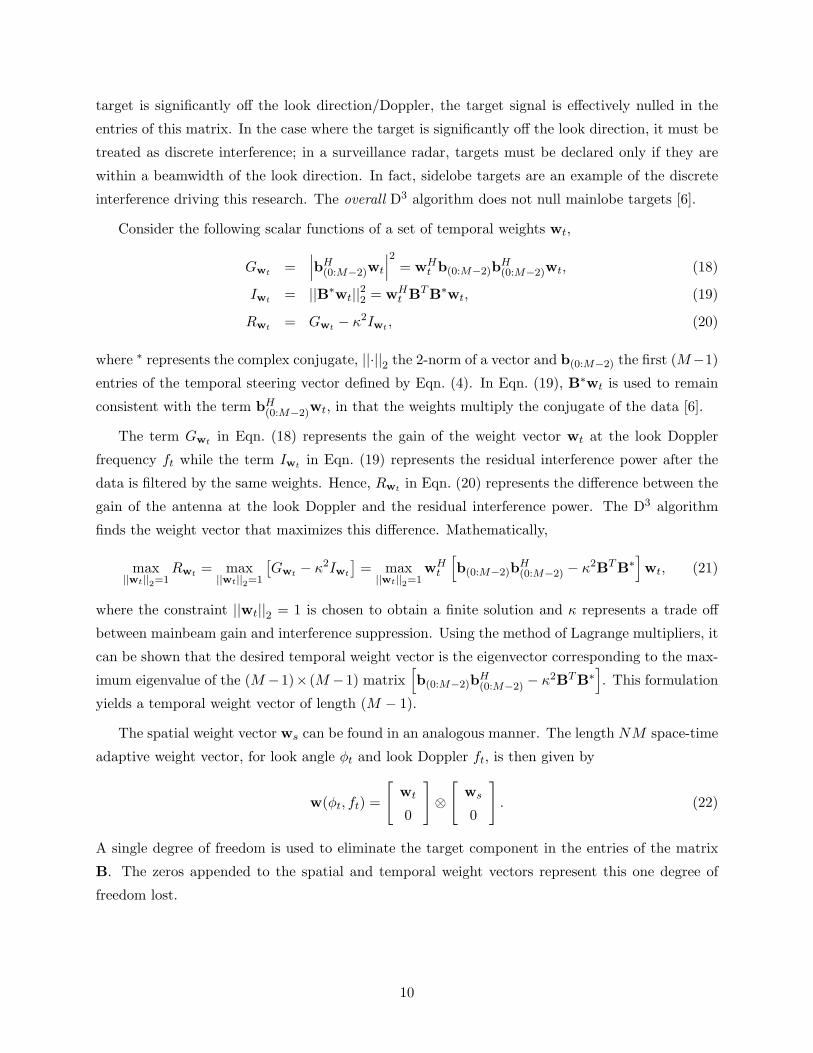
Fig. 7, correlate directly with major highways in Maryland and Delaware illuminated by the radar

mainbeam. Routes 290 and 301 in Maryland are closely spaced at a range of 9.0 and 9.8 miles.

Accounting for the platform motion, the ground speed of the target(s) is approximately 50 mph.

In essence the hybrid algorithm has been applied to all range/Doppler bins where the JDL-MSMI

statistic is greater than 18.52. The hybrid algorithm suppresses non-homogeneities, significantly

reducing false alarms. In addition, the weaker injected target is detected because the stronger

target at range bin 295 is eliminated from the sample support. Note that because the NHD does

not identify this range bin (range bin 290) as a non-homogeneity, the weak target is detected using

statistical JDL processing only because other homogeneous cells are used for sample support.

The target detections at the far range shown in the plot are between 19.4 and 20.4 miles. The

range to Route 9 varies between 19.1 and 21.1 miles within the transmit mainbeam. These far

range detections therefore correspond to Route 9. The targets detected at these ranges are present

in both Figs. 6 and 7.

3.2 Potential Enhancements to KB-STAP

The KB-processor presented here is the simplest formulation where the adaptive process is chosen

to match the interference within the primary range cell. The choice of the JDL-NHD and JDL as

the statistical algorithm is only one of several possible choices. This choice is made because of the

ease in implementation with all components dependent on the JDL algorithm. A more sophisticated

processor would choose from several possible statistical algorithms to maximize the probability of

detection for a given false alarm rate. For example, the choice could be from with the algorithm

presented here and the knowledge-based algorithms in [8–11].

The key difference between any KB-processor and traditional processing is the use of a knowl-

edge base. There are several sources that may inform this knowledge. As described by Antonik

et al. [20], some of the possible information sources are: elevation and cover data to distinguish

different terrains using a-priori map information so only secondary data from similar terrain is

used, other sensors of opportunity to key in on likely target locations, feedback from other stages

such as the tracker, information from other passes or flights to locate discrete non-homogeneities,

etc.

4 Conclusions

This paper furthers the development of knowledge-based adaptive processing for ground moving

target indication. Traditional statistical processing techniques are inadequate in real world situa-

tions due to array effects and non-homogeneous data. The theoretical developments presented here

19

are motivated by the need to apply STAP for GMTI in real world processors. This paper intro-

duces a KB-STAP algorithm where the adaptive process is chosen to best match the interference

at hand. The overall KB-STAP algorithm is based on STAP algorithms that account for real-world

effects such as mutual coupling between antenna elements. The result is a practical, comprehensive,

approach that addresses both theoretical and practical issues in implementing STAP for GMTI.

The development of the KB-processor required theoretical investigations into various aspects of

adaptive processing in real world arrays. The three essential topics addressed here are the use of

practical antenna arrays, the detection of non-homogeneous data, and adaptive processing within

the non-homogeneous cells. Though these issues have been discussed elsewhere, they are presented

here individually for completeness. They are then brought together into a single KB-processor.

Figure 1 represents only the essential elements of such a processor. This formulation is one

starting point for future improvements to the knowledge based processing concept. The signifi-

cant processing gains achievable using KB-processing drives interest in this relatively new area of

research.

References

[1] J. Ward, “Space-time adaptive processing for airborne radar,” Tech. Rep. F19628-95-C-0002,MIT Linclon Laboratory, December 1994.

[2] L. Brennan and I. Reed, “Theory of adaptive radar,” IEEE Transactions on Aerospace andElectronic Systems, vol. 9, pp. 237–252, March 1973.

[3] I. S. Reed, J. Mallett, and L. Brennan, “Rapid convergence rate in adaptive arrays,” IEEETransactions on Aerospace and Electronic Systems, vol. 10, No. 6, pp. 853–863, Nov. 1974.

[4] R. S. Adve, T. B. Hale, and M. C. Wicks, “Transform domain localized processing usingmeasured steering vectors and non-homogeneity detection,” in Proceedings of the 1999 IEEENational Radar Conference, pp. 285–290, Apr. 1999. Boston, MA.

[5] R. S. Adve, T. B. Hale, and M. C. Wicks, “Joint domain localized adaptive processing inhomogeneous and non-homogeneous environments. part I: Homogeneous environments,” IEEProceedings on Radar Sonar and Navigation, vol. 147, pp. 57–65, April 2000.

[6] R. S. Adve, T. B. Hale, and M. C. Wicks, “Joint domain localized adaptive processing inhomogeneous and non-homogeneous environments. part II: Non-homogeneous environments,”IEE Proceedings on Radar Sonar and Navigation, vol. 147, pp. 66–73, April 2000.

[7] D. E. Kreithen, N. B. Pulsone, C. M. Rader, and G. E. Schrader, “The MIT Lincoln LaboratoryKASSPER algorithm testbed and baseline algorithm suite,” in Proc. of 2002 Sensor Array andMultichannel Sig. Proc. Workshop, Aug. 2002.

[8] W. L. Melvin, G. A. Showman, and J. R. Guerci, “A knowledge-aided GMTI detection archi-tecture,” in Proc. of 2004 IEEE Radar Conference, Apr. 2004. Philadelphia.

20

[9] J. S. Bergin, C. M. Teixeira, P. M. Techau, and J. R. Guerci, “STAP with knowledge-aideddata pre-whitening,” in Proc. of 2004 IEEE Radar Conference, Apr. 2004. Philadelphia.

[10] M. Rangaswamy, F. C. Lin, and K. R. Gerlach, “Robust adaptive signal processing methodsfor heterogeneous radar clutter scenarios,” Signal Proc., vol. 84, pp. 1653–1665, Sept. 2004.

[11] S. Blunt, K. R. Gerlach, and M. Rangaswamy, “The enhanced FRACTA algorithm withknowledge aided covariance estimation,” in Proc. of 2004 Sensor Array and MultichannelSig. Proc. Workshop, July 2004.

[12] D. Sloper, D. Fenner, J. Arntz, and E. Fogle, “Multi-channel airborne radar measurement(MCARM), MCARM flight test,” Contract F30602-92-C-0161, Westinghouse Electronic Sys-tems, April 1996. Additional information available at http://sunrise.deepthought.rl.af.mil.

[13] L. Cai and H. Wang, “Performance comparisons of modified SMI and GLR algorithms,” IEEETransactions on Aerospace and Electronic Systems, vol. 27, No. 2, pp. 487–491, Apr. 1991.

[14] H. Wang and L. Cai, “On adaptive spatial-temporal processing for airborne surveillance radarsystems,” IEEE Transactions on Aerospace and Electronic Systems, vol. 30, pp. 660–699, July1994.

[15] H.-H. Chang, Improving Space-Time Adaptive Processing (STAP) Radar Performance in Non-homogeneous Clutter. PhD thesis, Syracuse University, August 1997.

[16] M. C. Wicks, W. L. Melvin, and P. Chen, “An efficient architecture for nonhomogeneitydetection in space-time adaptive processing airborne early warning radar,” in Proceedings ofthe 1997 International Radar Conference, pp. 295–299, October 1997. Edinburgh, UK.

[17] T. K. Sarkar and N. Sangruji, “An adaptive nulling system for a narrow-band signal witha look-direction constraint utilizing the conjugate gradient method,” IEEE Transactions onAntennas and Propagation, vol. 37, pp. 940–944, July 1989.

[18] S. Park and T. K. Sarkar, “A deterministic eigenvalue approach to space time adaptive process-ing,” in Proceedings of the IEEE Antennas and Propagation Society International Symposium,pp. 1168–1171, July 1996.

[19] T. K. Sarkar, S. Nagaraja, and M. C. Wicks, “A deterministic direct data domain approachto signal estimation utilizing non-uniform and uniform 2-d arrays,” Digital Signal Processing,vol. 8, pp. 114–125, April 1998.

[20] P. Antonik, M. C. Wicks, and Y. Salama, “Knowledge based radar signal and data processing,”in Proceedings of the 5th International Conference on Radar Systems, May 1999. Brest, France.

21