Embed Size (px)
Citation preview
KB-STAP Implementation for HFSWR
Contract Number: W7714-060999/001/SV
Maryam Ravan, Oliver Saleh, Raviraj S. Adve,Kostas Plataniotis and Petros Missailidis
Dept. of Electrical and Computer Engineering
University of Toronto
10 King’s College Road
Toronto, Ontario, M5S 3G4, Canada
{osaleh, rsadve, kostas}@comm.utoronto.ca ,
March 2008
Final Report

Abstract
This project deals with the development of knowledge based space-time adaptive processing (KB-STAP) techniques for high frequency surface wave radar (HFSWR). Target detection in HFSWRis fundamentally limited by ionospheric and sea clutter, both of which are well known to be highlynon-homogeneous. The goal is to develop an understanding the problem of ionospheric clutter, theformulation of knowledge based approaches to weak target detection, leveraging past work by theresearchers into KB-STAP for airborne radar (a significantly more benign problem).
This effort has addressed the problem of STAP for ionospheric clutter in a comprehensivemanner. Available STAP algorithms have been tested using measured HFSWR data. Two keycontributions of this effort have been the development of a data model of single-bounce ionosphericclutter and the development of an extremely efficient and effective STAP algorithm based on theFast Fourier Transform approach. It is our sincere belief that the effort undertaken has beenextremely successful.

Contents
1 Introduction 1
2 Preliminaries: Literature Review and Data Analysis 3
2.1 Literature Review of Data Analysis as Applied to HFSWR . . . . . . . . . . . . . . 3
2.1.1 Data Modeling . . . . . . . . . . . . . . . . . . . . . . . . . . . . . . . . . . . 4
2.2 Literature Review of Adaptive Processing as Applied to HFSWR . . . . . . . . . . . 5
2.3 Preliminary Data Analysis . . . . . . . . . . . . . . . . . . . . . . . . . . . . . . . . . 7
2.3.1 Element-Range Plots . . . . . . . . . . . . . . . . . . . . . . . . . . . . . . . . 8
2.3.2 Range-Doppler Plots . . . . . . . . . . . . . . . . . . . . . . . . . . . . . . . . 8
2.3.3 Angle Doppler Plots . . . . . . . . . . . . . . . . . . . . . . . . . . . . . . . . 11
2.4 Adaptive Processing . . . . . . . . . . . . . . . . . . . . . . . . . . . . . . . . . . . . 13
2.4.1 Data and Processing Model . . . . . . . . . . . . . . . . . . . . . . . . . . . . 13
2.4.2 Simulation Results . . . . . . . . . . . . . . . . . . . . . . . . . . . . . . . . . 16
2.5 KB-STAP . . . . . . . . . . . . . . . . . . . . . . . . . . . . . . . . . . . . . . . . . . 17
3 Data Models for Ionospheric Clutter 21
3.1 Data Model of Fabrizio [1] . . . . . . . . . . . . . . . . . . . . . . . . . . . . . . . . . 21
3.1.1 Signal Processing Model . . . . . . . . . . . . . . . . . . . . . . . . . . . . . . 21
3.1.2 Parameter Estimation . . . . . . . . . . . . . . . . . . . . . . . . . . . . . . . 23
3.2 Data Model of Riddolls [2] . . . . . . . . . . . . . . . . . . . . . . . . . . . . . . . . . 28
3.2.1 Path integral formulation of wave packet properties . . . . . . . . . . . . . . 29
3.2.2 Second-order statistics . . . . . . . . . . . . . . . . . . . . . . . . . . . . . . . 31
3.2.3 Modeling the Space-Time-Range Data Cube . . . . . . . . . . . . . . . . . . . 32
3.2.4 Simulation Results . . . . . . . . . . . . . . . . . . . . . . . . . . . . . . . . . 33
3.2.5 Summary . . . . . . . . . . . . . . . . . . . . . . . . . . . . . . . . . . . . . . 34
4 Space-Time Adaptive Processing of Ionospheric Clutter 40
4.1 Joint Domain Localized Processing . . . . . . . . . . . . . . . . . . . . . . . . . . . . 41
i

4.1.1 Simulation Results . . . . . . . . . . . . . . . . . . . . . . . . . . . . . . . . . 44
4.1.2 Discussion . . . . . . . . . . . . . . . . . . . . . . . . . . . . . . . . . . . . . . 51
4.2 The Direct Data Domain Algorithm . . . . . . . . . . . . . . . . . . . . . . . . . . . 55
4.3 The Hybrid Algorithm . . . . . . . . . . . . . . . . . . . . . . . . . . . . . . . . . . . 57
4.4 The Parametric Adaptive Matched Filtering Algorithm . . . . . . . . . . . . . . . . 58
4.5 Realistic Target Model . . . . . . . . . . . . . . . . . . . . . . . . . . . . . . . . . . . 64
4.5.1 Discussion on STAP Algorithms . . . . . . . . . . . . . . . . . . . . . . . . . 72
4.6 Fast Fully Adaptive Algorithm . . . . . . . . . . . . . . . . . . . . . . . . . . . . . . 74
4.6.1 System Model . . . . . . . . . . . . . . . . . . . . . . . . . . . . . . . . . . . . 75
4.6.2 Fast Fully Adaptive Algorithm . . . . . . . . . . . . . . . . . . . . . . . . . . 76
4.6.3 Complexity Analysis . . . . . . . . . . . . . . . . . . . . . . . . . . . . . . . . 79
4.6.4 Simulation Results . . . . . . . . . . . . . . . . . . . . . . . . . . . . . . . . . 83
4.7 Interleaved FFA Description . . . . . . . . . . . . . . . . . . . . . . . . . . . . . . . . 86
4.8 Complexity Analysis . . . . . . . . . . . . . . . . . . . . . . . . . . . . . . . . . . . . 90
4.8.1 Unequal Partitions . . . . . . . . . . . . . . . . . . . . . . . . . . . . . . . . . 91
4.8.2 Simulation Results . . . . . . . . . . . . . . . . . . . . . . . . . . . . . . . . . 94
4.8.3 Probability of Detection versus SNR . . . . . . . . . . . . . . . . . . . . . . . 94
4.9 Summary and Conclusions . . . . . . . . . . . . . . . . . . . . . . . . . . . . . . . . . 98
5 Conclusion 100
ii

List of Figures
2.1 Element-range power distribution for pulse number 1 . . . . . . . . . . . . . . . . . . 9
2.2 Element-range power distribution for pulse number 2000 . . . . . . . . . . . . . . . . 9
2.3 Range-Doppler power distribution for element number 1 . . . . . . . . . . . . . . . . 10
2.4 Range-Doppler power distribution for element number 8 . . . . . . . . . . . . . . . . 10
2.5 Range-Doppler power distribution for element number 13 . . . . . . . . . . . . . . . 11
2.6 Angle-Doppler power distribution for range bin 1 . . . . . . . . . . . . . . . . . . . . 12
2.7 Angle-Doppler power distribution for range bin 50 . . . . . . . . . . . . . . . . . . . 12
2.8 Angle-Doppler power distribution for range bin 100 . . . . . . . . . . . . . . . . . . . 14
2.9 Angle-Doppler power distribution for range bin 150 . . . . . . . . . . . . . . . . . . . 14
2.10 Angle-Doppler power distribution for range bin 200 . . . . . . . . . . . . . . . . . . . 15
2.11 Angle-Doppler power distribution for range bin 225 . . . . . . . . . . . . . . . . . . . 15
2.12 Output statistic with non-adaptive processing . . . . . . . . . . . . . . . . . . . . . . 18
2.13 MSMI statistic as a function of range and Doppler . . . . . . . . . . . . . . . . . . . 18
2.14 Comparing adaptive and non-adaptive processing with target within the Bragg line . 19
2.15 Comparing adaptive and non-adaptive processing with target within the ionosphericclutter . . . . . . . . . . . . . . . . . . . . . . . . . . . . . . . . . . . . . . . . . . . . 19
3.1 Real part of (a) noisy and (b) estimated autocorrelation function. . . . . . . . . . . . 25
3.2 Real part of (a) measured and (b) estimated autocorrelation function for range bin220. . . . . . . . . . . . . . . . . . . . . . . . . . . . . . . . . . . . . . . . . . . . . . 26
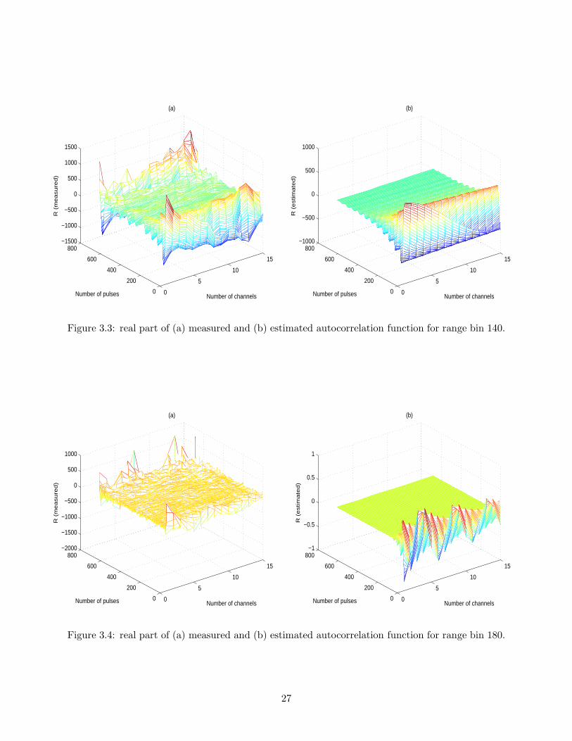
3.3 real part of (a) measured and (b) estimated autocorrelation function for range bin140. . . . . . . . . . . . . . . . . . . . . . . . . . . . . . . . . . . . . . . . . . . . . . 27
3.4 real part of (a) measured and (b) estimated autocorrelation function for range bin180. . . . . . . . . . . . . . . . . . . . . . . . . . . . . . . . . . . . . . . . . . . . . . 27
3.5 (a)Angle of arrival and (b) Doppler frequency spectrum for range bin 220. . . . . . . 28
3.6 (a)Angle of arrival and (b) Doppler frequency spectrum for range bin 140. . . . . . . 29
3.7 (a)Angle of arrival and (b) Doppler frequency spectrum for range bin 180. . . . . . . 29
3.8 (a) Phase power spectrum and (b) autocorrelation function of the signal. . . . . . . . 35
iii
3.9 (a) Real and (b) imaginary part of the simulated signal for the range bin 34 whenE(ϕ2) is a random value between 1 × 10² and 2 × 10² . . . . . . . . . . . . . . . . . . 35
3.10 (a) Real and (b) imaginary part of simulated signal for the range bin 12 when E(ϕ2)is a random value between 2 × 10² and 3 × 10² . . . . . . . . . . . . . . . . . . . . . 36
3.11 Angle-doppler plot of the simulated signal (a) for the range bins 34 and (b) 12. . . . 36
3.12 (a) Real and (b) imaginary part of measured signal for the range bin 230. . . . . . . 37
3.13 (a) Real and (b) imaginary part of measured signal for the range bin 260. . . . . . . 37
3.14 Angle-doppler plot of the measured signal (a) for the range bins 230 and (b) 260. . . 38
3.15 Doppler-range plot of the simulated signal (a) for antenna element 13 when E(ϕ2)is in the range of (1 ∼ 2) × 102 and (b) for antenna element 6 when E(ϕ2) is in therange of (2 ∼ 3) × 102. . . . . . . . . . . . . . . . . . . . . . . . . . . . . . . . . . . . 38
3.16 Doppler-range plot of the measured signal (a) for antenna element 6. . . . . . . . . . 39
3.17 Doppler plot of the (a) simulated signal of range bin 12 and antenna element 6 and(b) measured signal of range bin 230 and antenna element 6 . . . . . . . . . . . . . . 39
4.1 A linear array of point sensors . . . . . . . . . . . . . . . . . . . . . . . . . . . . . . . 41
4.2 Localized processing regions in Joint Domain Localized processing. . . . . . . . . . . 43
4.3 ∆MSMI versus angle and Doppler spacing (ηa = ηd = 3). Ionospheric clutter region. 46
4.4 ∆MSMI versus angle and Doppler spacing (ηa = ηd = 3). Bragg region. . . . . . . . 47
4.5 ∆MSMI versus angle and Doppler spacing (ηa = 3, ηd = 5). Ionospheric clutter region. 47
4.6 ∆MSMI versus angle and Doppler spacing (ηa = 3, ηd = 5). Bragg region. . . . . . . 48
4.7 MSMI statistic (in dB) versus the range cell number for (ηa = ηd = 3). Ionosphericclutter region. . . . . . . . . . . . . . . . . . . . . . . . . . . . . . . . . . . . . . . . . 49
4.8 MSMI statistic (in dB) versus the range cell number for (ηa = ηd = 3). Bragg region. 50
4.9 MSMI statistic (in dB) versus the range cell number for (ηa = 3, ηd = 7). Ionosphericclutter region. . . . . . . . . . . . . . . . . . . . . . . . . . . . . . . . . . . . . . . . . 50
4.10 MSMI statistic (in dB) versus the range cell number for (ηa = 3, ηd = 7). Bragg region. 51
4.11 MSMI statistic (in dB) versus (in dB) versus the range cell number for (ηa = 3, ηd =7). Using all range cells in ionospheric clutter region. . . . . . . . . . . . . . . . . . . 52
4.12 A range-Doppler plot of the data-square containing obvious targets. The targets arespread over up to 15 ranges and are at Doppler bin numbers 89, 106, 131, and 151respectively. . . . . . . . . . . . . . . . . . . . . . . . . . . . . . . . . . . . . . . . . . 64
4.13 A power profile plot of the identified targets at Doppler bin numbers 89, 106, 131,and 151 respectively. . . . . . . . . . . . . . . . . . . . . . . . . . . . . . . . . . . . . 65
4.14 Results of using the JDL, Adaptive Doppler filter, and Nonadaptive MF algorithmsto detect an ideal target with amplitude 35dB inserted into the Ionospheric clutterregion. . . . . . . . . . . . . . . . . . . . . . . . . . . . . . . . . . . . . . . . . . . . . 67
4.15 Results of using the JDL, Adaptive Doppler filter, and Nonadaptive MF algorithmsto detect an ideal target with amplitude 45dB inserted into the Ionospheric clutterregion. . . . . . . . . . . . . . . . . . . . . . . . . . . . . . . . . . . . . . . . . . . . . 67
iv

4.16 Results of using the JDL, Adaptive Doppler filter, and Nonadaptive MF algorithmsto detect a real target spread over 7 range cells and with amplitude 57dB insertedinto the Ionospheric clutter region. . . . . . . . . . . . . . . . . . . . . . . . . . . . . 68
4.17 Results of using the D3, Spatial Adaptive Doppler filter, and Nonadaptive MF algo-rithms to detect an ideal target with amplitude 55dB inserted into the Ionosphericclutter region. . . . . . . . . . . . . . . . . . . . . . . . . . . . . . . . . . . . . . . . . 70
4.18 Results of using the D3, Spatial Adaptive Doppler filter, and Nonadaptive MF al-gorithms to detect a real target spread over 7 range cells and with amplitude 55dBinserted into the Ionospheric clutter region. . . . . . . . . . . . . . . . . . . . . . . . 71
4.19 Results of using the Hybrid,D3,JDL, Spatial Adaptive Doppler filter, and Nonadap-tive MF algorithms to detect an ideal target with amplitude 55dB inserted into theIonospheric clutter region. . . . . . . . . . . . . . . . . . . . . . . . . . . . . . . . . . 72
4.20 Results of using the Hybrid,D3,JDL, Spatial Adaptive Doppler filter, and Nonadap-tive MF algorithms to detect a real target spread over 7 range cells and with ampli-tude 55dB inserted into the Ionospheric clutter region. . . . . . . . . . . . . . . . . . 73
4.21 Results of using the RSC-PAMF, TASC-PAMF, Adaptive Doppler filter, and Non-adaptive MF algorithms to detect an ideal point target with amplitude 59dB insertedinto the Ionospheric clutter region. . . . . . . . . . . . . . . . . . . . . . . . . . . . . 74
4.22 Results of using the RSC-PAMF, TASC-PAMF, Adaptive Doppler filter, and Non-adaptive MF algorithms to detect a real target spread over 7 range cells and withamplitude 63dB inserted into the Ionospheric clutter region. . . . . . . . . . . . . . . 75
4.23 A tree-like representation of the FFA method for a datacube with M = 12 pulses,N = 12 elements, spatial-partitioning-sequence=[2 2 1 3], and temporal-partitioning-sequence=[4 1 3 1]. . . . . . . . . . . . . . . . . . . . . . . . . . . . . . . . . . . . . . 80
4.24 ∆MSMI versus target amplitude for JDL, and FFA algorithms . . . . . . . . . . . . 85
4.25 MSMI vs Range plots for using the Nonadaptive, JDL, and FFA methods to detectan ideal target in Ionospheric clutter region. All 4096 pulses are used in this simulation. 86
4.26 MSMI vs Range plots for using the Nonadaptive, JDL, and FFA methods to detect anideal target in Ionospheric clutter region. Only 128 pulses are used in this simulation. 87
4.27 MSMI vs Range plots for using the Nonadaptive, JDL, and FFA methods to detecta real target in Ionospheric clutter region. All 4096 pulses are used in this simulation. 88
4.28 MSMI vs Range plots for using the Nonadaptive, JDL, and FFA methods to detecta real target in Ionospheric clutter region. Only 128 pulses are used in this simulation. 89
4.29 A representation of the Interleaved-FFA method. . . . . . . . . . . . . . . . . . . . . 90
4.30 Probability of detection versus SNR for a PFA=0.1, using JDL, regular FFA, andinterleaved FFA methods. . . . . . . . . . . . . . . . . . . . . . . . . . . . . . . . . . 95
4.31 MSMI versus range plot for interleaved-FFA method using 4096 pulses in an idealtarget scenario . . . . . . . . . . . . . . . . . . . . . . . . . . . . . . . . . . . . . . . 96
4.32 MSMI versus range plot for interleaved-FFA method using 4096 pulses in a realtarget scenario . . . . . . . . . . . . . . . . . . . . . . . . . . . . . . . . . . . . . . . 96
4.33 MSMI versus range plot for interleaved-FFA method using 128 pulses in an idealtarget scenario . . . . . . . . . . . . . . . . . . . . . . . . . . . . . . . . . . . . . . . 97
v

4.34 MSMI versus range plot for interleaved-FFA method using 128 pulses in a real targetscenario . . . . . . . . . . . . . . . . . . . . . . . . . . . . . . . . . . . . . . . . . . . 97
4.35 ∆MSMI versus target amplitude for JDL, FFA, and interleaved-FFA algorithms . . 98
vi

Chapter 1
Introduction
The overall goal of this project is to develop a knowledge based space-time adaptive processing(KB-STAP) approach to deal with the non-homogeneous interference in high frequency surfacewave radar (HFSWR). Performance of target detection algorithms, especially non-adaptive tech-niques, in HFSWR are primarily limited by sea clutter (at the near ranges) and ionospheric clutter(at the far ranges). In this regard, STAP appears to be a promising approach to deal with suchinterference. However, traditional STAP algorithms fundamentally assume the interference to bespatially homogeneous, i.e., that the statistics of the interference are consistent as a function ofrange. STAP algorithms, initially developed in the context of airborne surveillance radar, exploitthis homogeneity to estimate interference statistics for clutter suppression. Specifically these statis-tics are estimated by averaging over the homogeneous range cells. Sea and ionospheric clutter, onthe other hand, are well known to be highly non-homogeneous, requiring the development of al-ternative STAP approaches. However, our previous work [3, 4] suggested that the fundamentallimiting factor in the available ionospheric clutter data sets is the lack of secondary range cells toestimate the interference covariance matrix.
In the field of STAP for airborne radar, a significant development is a knowledge based approachwherein information extracted in real time [5, 6] is exploited to determine the choice of adaptivealgorithm, the parameters of the algorithm and the choice of range cells in the estimation process.The fundamental motivation in KB-STAP is the clutter non-homogeneity in airborne radar. Inthis regard, one key building block to this KB=STAP approach is the hybrid algorithm of [7]which combines the benefits of direct data domain (D3) and statistical processing. By tailoringthe algorithm, and its parameters, to the interference within a specific range cell, KB-STAP hasthe potential for making a greater impact on target detection in HFSWR. Fundamentally, ”theobjective of this project is to formulate and evaluate practical KB-STAP algorithms for detectionof surface vessels in strong ionospheric clutter by the Canadian East Coast HFSWRs”, a phraseextracted from the contract. As we will see, the issue clutter non-homogeneity was addressed by thedevelopment of a new adaptive algorithm tailored to fit the special characteristics of the HFSWRdataset.
This project, as is this report, was broadly divided into three phases: a literature survey andfamiliarization phase, a modeling and analysis phase and, finally, a formulation and testing phase.The first phase, which was documented in a report submitted in late-March 2007, presented asurvey of the available literature in the area of modeling and adaptive processing of ionosphericclutter [8]. That report also presented results of some preliminary implementations of space-timeadaptive processing without any regard to clutter non-homogeneities. Given the limited training
1
samples available, the implementation was based on a factored approach, using a non-adaptiveestimate in the Doppler dimension and restricting adaptive processing to the spatial dimensiononly.
In the second stage we began the formulation of a data model of ionospheric clutter. The modelthen focused on the work of Fabrizio [1] which presents a preliminary data model for ionosphericclutter observed via a over-the-horizon radar system. Unfortunately, the data provided by theDefense Research and Development Canada (DRDC) does not follow the model of [1]. In ourJune 2007 report [3] we showed that when applying the data model, the parameters that arise arephysically impossible.
These progress reports [3,4] also detailed our preliminary efforts in applying space-time adaptiveprocessing (STAP), including the hybrid approach to the data sets provided by DRDC. The resultsshowed the significant gains possible in using STAP when detecting weak targets; targets thatcould not be detected using non-adaptive processing stand out by as much as 10-15dB when usingadaptive processing. A crucial issue identified in previous work is the issue of sample support. Allthe data sets provided by DRDC can be divided into three segments: one dominated by the Bragglines, one by homogeneous clutter and one dominated by ionospheric clutter. Since only data thatis representative of the interference can be used to estimate the interference covariance matrix,the progress report in June 2007 focused heavily on the joint domain localized (JDL) processingalgorithm [9,10]. The report in September 2007 [4] presented the use of the hybrid algorithm.
The December 2007 progress report [11] detailed the development of a data model based onthe work of [2]. This model developed by Dr. Ravan, in conjunction with significant input fromDr. Ryan Riddolls of DRDC, is able to match the characteristics of the measured data. ThisDecember report also presented a new adaptive processing algorithm that is able to exploit theentire space-time data set with limited training. The algorithm is based on the FFT, was dubbedthe Fast Fully Adaptive (FFA) approach. We emphasize that these two aspects of the Decemberreport are the two key contributions of this effort. In this final report we describe testing andgeneralization of the FFA algorithm, material not described in any report earlier.
This final report compiles the information contained in our previous progress reports and de-tails the final testing phase of the project. In some places therefore, there is some repetition ofinformation, though this has been kept to a minimum to facilitate understanding of the materialin each chapter. The report is organized as follows: Chapter 2 reviews the preliminary work un-dertaken in this effort. This chapter covers a literature review of relevant work and the resultsof some preliminary adaptive and non-adaptive data analysis for the measured HFSWR dataset.Chapter 3 presents one of the core contributions of this effort - a data model to simulate ionosphericdata. Chapter 4 presents results of all the space-time adaptive processing schemes developed andimplemented in this chapter. Of special importance are Sections 4.6 and 4.7 that present the newadaptive algorithm developed under this effort. These schemes are shown to provide huge improve-ments over any of the other STAP algorithms implemented. The report concludes with severalremarks on the overall effort in Chapter 5.
2

Chapter 2
Preliminaries: Literature Review andData Analysis
This chapter deals with the first phase in the project: the literature survey and familiarizationphase. This chapter covers the specific tasks:
• Literature survey of the available public domain work on data analysis for HFSWR.
• Literature survey of STAP algorithms as applied to HFSWR.
• Preliminary data analysis of the HFSWR data set provided by the Defense Research andDevelopment Canada (DRDC) Technical Authority, Dr. Ryan Riddolls.
• Identification of source of information for anticipated application of KB-STAP.
The goal of the first phase was largely, therefore, for the researchers to familiarize themselveswith the available literature and to set the stage for following two phases.
This chapter is organized as follows: Section 2.1 provides an overview of the available literaturein data gathering and modelling of HFSWR data, especially ionospheric clutter. Section 2.2 presentsa similar review of data analysis and adaptive processing as applied to HFSWR. Section 2.3 presentsthe results of our preliminary non-adaptive data analysis of the data set provided by Dr. Riddolls.Section 2.4 presents the methodology and results of the preliminary adaptive processing work.Section 2.5 focuses on our suggestions in how to apply KB-STAP to HFSWR.
2.1 Literature Review of Data Analysis as Applied to HFSWR
In mitigating the deleterious effects of ionosphere clutter in target detection with the incorpora-tion of HFSWR there is no consensus amongst researchers on the optimal approach. There is avariety of factors that can influence the efficacy of the algorithms and their applicability dependson the particulars of the ionosphere prevailing in a certain location. The non-stationarity and non-homogeneity properties that characterize the ionosphere provide additional intellectual challengesin contriving reliable, ubiquitously applicable mathematical models. The synergy of selection ofvalidated models tailored to the peculiarities of a particular location, space-time processing modal-ities to extract the information of interest and effective decision making paradigms is imperative inaddressing the issue.
3

There exist a few groups of researchers with the needed experimental facilities that appearto have dominated the area of signal processing for ionospheric clutter. These groups have beenidentified, the latest propensities have been examined and segments of their produced work isincluded in an attempt to incorporate the most relevant and recent accomplishments. The timelimitations conduced to the deficiency of presenting the findings in a systematic and pragmaticmanner. A synopsis of various papers is presented highlighting limitations and strengths.
In [12] the authors deal with phase contamination due to ionospheric clutter. The specific prob-lem is that the Doppler spread mechanism renders the sea clutter spectrum distorted and resolutionof coherent integration technique is degraded tremendously. In surface surveillance and remote sens-ing, temporal nonlinear phase path variations often produce significant spread of the ionosphericpropagated signals so that the Bragg lines and the target echoes smear cross the Doppler frequencydomain masking slow moving surface surface vessels. The phase contamination is attributed tocomplex geophysical mechanisms. The authors approach is based on estimating the instantaneousfrequency, modelling the phase contamination by a polynomial phase. They make significant im-provement in spectrum quality.
In [13] the same set of authors deal with double ionosphere transit. Bourdillon [14] suggestedcorrecting the phase of the signal from a perturbation estimated using maximum entropy spectralanalysis (MESA) as an estimator for the quasi-instantaneous frequency of the Bragg lines with time.It is likely to fail for the contamination with periods shorter than a few tens of a second integrationtime that is used in the autoregressive spectral estimation process. Perent and Bourdillon [15]proposed a simpler technique using time derivative of the signal phase as the estimation of theinstantaneous frequency of the contamination with short periods. This method has introducedinitially the concept of multiple operating frequencies but it is not suitable for regular FMCWradar due to its complexity.
Abramovich, Anderson and Soloman [16] addressed another method based on eigenvalue de-composition. It is an advanced version of noise subspace technique applied to the instantaneousfrequency estimation. However, since the correlation between the adjacent range, azimuth, and fre-quency bins of the echo signal is unknown and varying, the autocorrelation matrix estimated fromthe available data set may be biased or rank-deficient. Thus the eigen-decomposition techniqueunder these conditions is defective or even ineffective. An improved scheme is presented to com-pensate nonlinear phase path contamination, when the backscattered signal propagates through theionosphere in high-frequency sky-wave radar systems, though not the surface wave radar systemwe consider in this project.
2.1.1 Data Modeling
The central aim of this project is the development and testing of STAP algorithms for HFSWR. Itis therefore essential to have available both measured data, but also simulated data to develop andtest algorithms in a controlled environment.
In terms of data modeling, in [17], the authors simulate ionospheric scintillation. The iono-spheric plasma may be treated as an electron density with variation on both in space and time.Two general types of effects are produced at radar; the measurement of range is affected because ofdeviations of the speed of light in the refractive medium with direct ramification on radar’s trackingfunction. It is the large-scale structure of the electron density that governs the range effects. Thesecond effect is scintillation that occurs because of the existence of interfering optical paths betweenthe target and the radar. Scintillation is produced by electron density structures on the size scale of
4

the radar wavelength, and therefore tends to vary rapidly due to small motions of the radar-targetpath or changes in the medium. For key radar functions like object classification, scintillation isthe effect which causes performance degradation. However, this may not play as significant a rolein target detection.
From our literature survey, there appear to be two different approaches to modeling ionosphericand sea clutter. Our initial analysis suggested that one important and useful model has beendeveloped by Fabrizio in his Ph.D. thesis [1]. He verifies the accuracy of space-time wave interferencemodels and uses this theory to develop a space-time model of ionospheric clutter returns and alsoprovides a parameter estimation technique to fit measured data into the model. This model is validfor a coherent pulse interval (CPI) shorter than a few seconds. For longer CPIs, he develops astationary statistical model focusing on the prediction of second order statistics. The ionosphericreflections are treated as a random variable (unlike the wave interference model initially developed).He proposes hypothesis tests to accept or reject the validity of the model given measured data.
One should emphasize that the experimental data used by Fabrizio is taken from Jindalee radarrun, apparently, by the Defense Science and Technology Organization (DSTO) in Australia. Therewas no guarantee that this model will be applicable to the Cape Race HFSWR. Furthermore, asindicated by Dr. Riddolls, the model used by Fabrizio is rather simplistic, dependent on a Gaussianassumption which is not valid in practice. The more commonly accepted distribution is based onfourth-order power law, making the power distribution fall off much slower than the Gaussian. Weattemptted to modify Fabrizio’s model to make it more realistic, but our efforts were unsuccessful.
An alternative approach also from DSTO is that of Coleman [18,19]. This model was recentlyextended by Dr. Riddolls [20, 21] to simultaneously account for group delay, direction of arrival,location and Doppler. The author uses a ray tracing model and treats irregularities as perturbationsof a “quiescent” path solution without irregularities. At first glance this model seems considerablymore complicated than that of Fabrizio. However, we will attempt to implement both schemes andcompare their fidelity given data sets from DRDC.
A comprehensive analysis of ionospheric clutter is by Chan [22] which can be used for modeltesting. This work also contributed to a detailed report by Sevgi et al. [23, 24] where a stochasticmodel package called HFSIM [25] is discussed. This package is also based on a Gaussian assumption.Another stochastic model is that of [26].
In summary, there are a few competing approaches to modelling ionospheric clutter. Our goalis to implement an accurate, if more complex data model. In this effort, the model of Fabrizio wasinvestigated in some detail and the model of Riddolls was finaly implemented.
2.2 Literature Review of Adaptive Processing as Applied to HF-SWR
This section reviews some of the work in adaptive processing for HFSWR. While several of thepapers were suggested to us by the DRDC Technical Authority, there are others works reviewedbelow, including some recent work of Fabrizio and Farina. Largely the work appears to havefocused on reducing the degrees of freedom in the processing scheme to reduce computation loadand requirements of statistically stationary sample support.
Some of the early works by researchers at DRDC include [27, 28] which discuss the use ofhorizontal dipoles as auxiliary antennas, as sidelobe cancellers, to suppress skywave interference.
5

The author finds the adaptive weights to optimally suppress interference. A reference signal isadded; we believe to obtain the weights using a Weiner solution. In [29] the author extends this toa comparison of the use of horizontal and vertical dipoles for interference suppression. The authorsuggests use of horizontal polarization to cancel interference close to the target location (whosesignal is vertically polarized). This work may not have significant impact on the present projectsince the measured data provided all uses the same (vertical) polarization.
Other efforts within DRDC, made available by Dr. Riddolls, include the coherent side cancellerwork of [30] where the authors investigate the optimal ordering of Doppler processing, beamform-ing and interference cancellation. One unfortunate, but not surprising result is that the optimalordering is interference dependent (and hence time dependent) since in HFSWR the interferencesources are highly time variant. A similar result was demonstrated in the context of airborne radarin [9]. In [30] specifically, the sidelobe canceller is shown effective against a single spatially confinedsource. An interesting, and sobering, presentation in this paper is the demonstration of the widespatial and temporal variation in the ionospheric clutter characteristics.
These works would, we believe, be considered “classical” in the space-time adaptive processingcommunity. They underline the complexity of the problem being attempted in this project and theneed for knowledge-based approaches. One should mention that our search of the DRDC databasegenerated several reports on direction finding for HF radar systems, a body of knowledge notreviewed here. One should also mention that there is continuing work in DRDC into the physicsand modeling of ionospheric clutter [20,21], work that played an important role in the next phaseof our project.
A significant fraction of the work adaptive processing for HFSWR is apparently led by Dr.Yuri Abramovich and/or Dr. Giuseppe Fabrizio at DSTO (though Fabrizio has recently startedalso collaborating with researchers in Italy such as Dr. Alfonso Farina). In particular, Fabriziohas several contributions developed in detail in his thesis and then several later works that arereviewed below. The work of Abramovich focuses largely on the underlying phenomenology andmeasurements [31].
The work of Fabrizio [1] is one focus of our proposed modelling and analysis approach. Thework of the group led by Fabrizio [1, 32–36] has focused on the development of the adaptive co-herence estimator (ACE) and its variant the spatial adaptive subspace detector (ASD) [32] forover-the-horizon (OTH) radar systems. In the following we largely focus on their most recentcontributions [34–36] presented as an improvement on their previous work [1, 32,33].
The ACE test, like the modified sample matrix inversion (MSMI) statistic, has the importantproperty of constant false alarm rate (CFAR); however ACE has the CFAR property even if the datawithin the range cell under test has a different scale from that in the secondary data. Unfortunately,ACE is highly susceptible to target mismatch and hence the motivation for the development of theASD detector. The ASD detector treats a single target as a signal subspace with rank greater than1 [35]. In their latest work [36], Fabrizio et al. address the issue of unwanted signals in the primary
data. They propose a generalized likelihood ratio test (GLRT) to address this issue. To address theissue of target mismatch, they model both the target and the discrete interference source withinthe primary range cell as low-rank sources given by a linear combination of closely spaced Dopplerfrequencies. The GLRT is then formed by maximizing over the parameters of both the targetand discrete interference. Unfortunately, a significant drawback is that the implementation of theGLRT requires exact knowledge of the parameters of the interference. This necessitates a two-passapproach wherein the the detector acquires some knowledge of the existence of the interference andits parameters in real time.
6

This two-pass approach is reminiscent of the two-pass approach proposed by Adve et al. in [5,6].We will revisit this issue later in this document in Section 2.5. It should be noted that other thanthe experimental results, the formulation in [36] does not specifically target HFSWR.
The work in [36] focuses on adaptive Doppler processing exclusively. Previously the authorsdeveloped a space-time adaptive processing algorithm [34] for OTH radar using beamspace-rangeprocessing. This paper is of interest because the authors claim that with N spatial elements andM time taps, they can reduce the dimension of the STAP filter to M + N as opposed to the usualMN . The move to beamspace is as in the joint domain localized processing scheme of [10] in thatthe spacing between beams is not restricted the use of a FFT. Interestingly, the authors use fast
time samples to form the Doppler steering vector, not the traditional slow time samples - hencebeamspace-range processing.
The other significant group of researchers working in adaptive processing for HF radar is inChina. In [37] the authors propose a scheme for clutter mitigation that both varies the clutterweights to counter non-stationary ionospheric clutter within a coherent processing interval (CPI)while maintaining some stability in the gain on target. Two issues with this paper appear to bethe need for partitioning the overall CPI in to sub-CPIs, increasing the computation load andthe somewhat ad-hoc nature of the proposed processing scheme with transitions from sub-CPI tosub-CPI.
The paper [38] is the basis for experimental work reported in [39]. In [38] the authors claimthat clutter and target only impacts on positive frequencies, not on negative frequencies. The basisfor this is not clear and will be investigated as we move forward in this project.
In [40] the authors present a multiple matched filtering scheme to deal with clutter multipathspecifically. Here the authors use the linear FM rate to distinguish the multiple paths and thecenter frequency to distinguish reflections from multiple layers. In this regard, this paper does notappear to be directly related to our work.
In [41] a ionospheric phase decontamination scheme using the singular value decomposition of aHankel matrix created out the received signal is proposed. This decontamination is then combinedwith suppression of sea clutter by removing the eigenvalues associated with the narrowband Bragglines. There is no adaptive processing in the sense proposed here in this project.
Beyond the groups reviewed above, a few other papers are available in the literature. For OTHsystems, the authors of [42] propose to distinguish between sea clutter and the target using acoherence function. Again, no adaptive processing of the type proposed here is performed. In [43]the authors extend temporal only processing to the use of STAP. However, the approach used isthe classic STAP approach of estimating the covariance using secondary data without any specificattention paid to homogeneity.
2.3 Preliminary Data Analysis
This section details the non-adaptive data processing conducted on the data set provided by theDRDC Technical Authority, Dr. Ryan Riddolls; the data set is hfswr data 25mar2002 030257.mat.The data comprises N = 16 channels, M = 4096 pulses, and K = 270 range cells. The radar operat-ing frequency was 3.1MHz corresponding to a wavenumber of k = 0.065rad/m. The first range cellcorresponds to 62.75km with each range cell covering 1.5km. The 4096 pulses use a pulse repetitionfrequency (PRF) of 15.625Hz, setting the maximum resolvable Doppler frequency to ±7.8125Hz.
7

The inter-element distance of the uniform linear array is d = 33.33m (corresponding to 0.344λ).
The data analysis conducted in this phase of the project focused on non-adaptive processing.Some sample results are provided illustrating the interference distribution as a function of angle,Doppler and range.
2.3.1 Element-Range Plots
The first set of results focus on the range dependence of the interference.
Figure 2.1 plots the power distribution, in dB, of the first pulse as a function of element andrange. There appear to be three distinct segments in range - a near range segment up to ap-proximately range cell 50 with significant interference power, a segment between range cell 50 and180 with lower power and, finally, the range cells dominated by ionospheric clutter past range cell180. The angle-Doppler plots associated with these range cells show an interesting variation in theangle-Doppler structure of the interference in these range segments. Figure 2.2, focusing on pulsenumber 2000, provides another plot to confirm this impression.
The figures also point to a problem with element 13, an issue pointed out by Dr. Riddolls. Thiselement appears to be attenuated by as much as 40dB. However, interestingly, focusing on thisone element suggests that this receiver is not totally “dead”. The associated angle-Doppler plot inFig. 2.5 presented later has the appropriate characteristics, only attenuated by as much as 40dB.
2.3.2 Range-Doppler Plots
This section focuses on range-Doppler plots for individual elements. In a large part these plotswere created using a snippet of MATLABr code received from Dr. Riddolls. The only changemade was in the labelling of the axis in terms of Doppler frequency and distance as opposed toDoppler/range bin. Figures 2.3 and 2.4 plot the power distribution of the radar signal returns asa function of range and Doppler. As is clearly seen, there are three distinct clutter regions; thenear region extending to approximately 200km (comprising approximately the first 50 range bins)dominated by the Bragg lines and sea clutter, a region at the far ranges beyond 350km dominatedby the ionospheric clutter and, interestingly, a middle region of sea clutter with less structure. Thiscorroborates with our initial impression from Figs. 2.1 and 2.2. As we will see in later plots, thisvariation in clutter structure is also visible in the angle-Doppler plots presented in Section 2.3.3and may have significant implications for interference suppression.
In both plots the Bragg lines are clearly visible. The advancing and receding lines are at±0.18Hz corresponding to the expected Doppler frequency given by
fB =
√g
πλ, (2.1)
where g = 9.81m/s2 is the acceleration due to gravity and λ is the wavelength corresponding tothe operating frequency of 3.1MHz.
The color bar on Figs. 2.3 and 2.4 corresponding to element 1 and element 8 also show a slighttaper between the edge element (1) and the center element (8). This was reported to us by Dr.Riddolls. Finally, another interesting plot is Fig. 2.5 with the range-Doppler power distribution forelement 13. While our initial understanding was that this channel was “dead”, in fact it appearsto be receiving data, but attenuated by as much as 40dB with respect to the other elements. At
8

50 100 150 200 250
2
4
6
8
10
12
14
16
Range #
Ele
men
t #
Element−range power (in dB) for pulse # 1
−10
0
10
20
30
40
50
Figure 2.1: Element-range power distribution for pulse number 1
50 100 150 200 250
2
4
6
8
10
12
14
16
Range #
Ele
men
t #
Element−range power (in dB) for pulse # 2000
−10
0
10
20
30
40
50
Figure 2.2: Element-range power distribution for pulse number 2000
9

Doppler in Hz
Ran
ge in
km
Range Doppler power plot (in dB) for element number 1
−0.8 −0.6 −0.4 −0.2 0 0.2 0.4 0.6 0.8
100
150
200
250
300
350
400
450
65
70
75
80
85
90
95
100
Figure 2.3: Range-Doppler power distribution for element number 1
Doppler in Hz
Ran
ge in
km
Range Doppler power plot (in dB) for element number 8
−0.8 −0.6 −0.4 −0.2 0 0.2 0.4 0.6 0.8
100
150
200
250
300
350
400
450
70
75
80
85
90
95
100
105
Figure 2.4: Range-Doppler power distribution for element number 8
10

Doppler in Hz
Ran
ge in
km
Range Doppler power plot (in dB) for element number 13
−0.8 −0.6 −0.4 −0.2 0 0.2 0.4 0.6 0.8
100
150
200
250
300
350
400
450
30
35
40
45
50
55
60
65
Figure 2.5: Range-Doppler power distribution for element number 13
the present time, for purposes of the adaptive processing scheme given below, we have eliminatedthis channel from the data. While it is not clear how to use channel 13, we may wish to retain thisflexibility in the future.
The range-Doppler plots provide crucial information for the STAP process. A fundamentallimitation of STAP is the need for training data to estimate the statistics of the interference with aprimary range cell. This training data, clearly, must be statistically homogeneous with respect tothe range cell under test. The range-Doppler plots indicate that there is limited training availablewithin each clutter region. This is independent of whether the clutter homogeneous within each ofthe three clutter regions described above.
2.3.3 Angle Doppler Plots
The final set of non-adaptive processing of the data provided by DRDC are angle-Doppler plots forindividual range cells. These plots are useful since they illustrate the power distribution in angle-Doppler space, the two Fourier spaces corresponding to the spatial and temporal domains in whichSTAP will be implemented. It is well accepted that it is easier to suppress localized interference(localized near a specific Doppler/angle). We will see that the range cells dominated by the Bragglines and those dominated by the ionospheric clutter appear to have a more coherent structure.
Figures 2.6 and 2.7 plot the angle-Doppler structure for range bins 1 and 50 respectively (rangesof 62.75km and 136.25km respectively). As is clear from Fig. 2.6 the interference in the first rangebin has a clear structure - the Bragg lines near zero Doppler are visible across all angles. Also, theinterference is localized to a few angles including a relatively strong source at approximately 35o
11
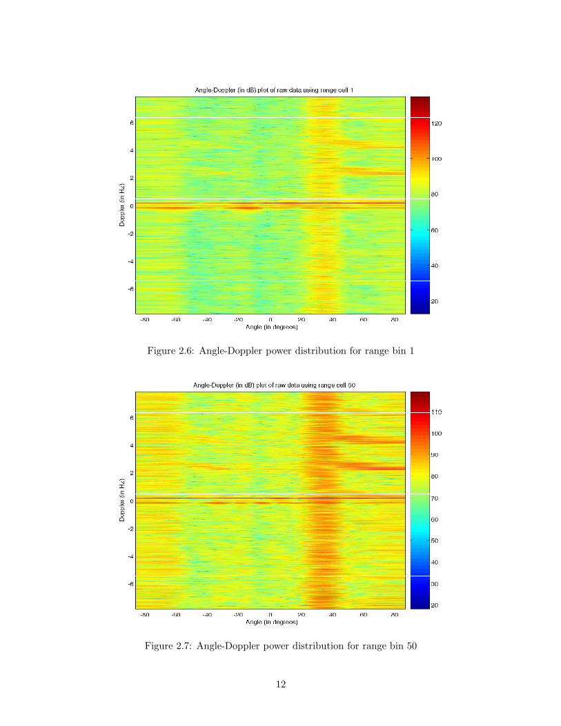
Figure 2.6: Angle-Doppler power distribution for range bin 1
Figure 2.7: Angle-Doppler power distribution for range bin 50
12

(relative to broadside). As well see, this interference source appears in all range cells 1. In additionto the Bragg lines, there appear to be two strong sources of interference near end-fire with Dopplerfrequency of approximately 4Hz. We have not, as of now, identified this source.
Figure 2.7 plots the power distribution in angle and Doppler for range cell 50, at the edgeof the first interference region. Comparing this plot to Fig. 2.6 one can see visualize the loss ofstructure in the interference. The interference here is far more spread out. This effect is furtherillustrated in Figs. 2.8 and 2.9 corresponding to range bins 100 and 150. In these two figures thelack of structure in the clutter is particularly striking. This has significant implications for theSTAP process; with its focus on a localized region in angle-Doppler space, an algorithm such asthe joint domain localized (JDL) processing scheme [9,10] may be useful here.
In the range cells dominated by ionospheric clutter, a structure is again visible in angle-Dopplerspace. Figures 2.10 and 2.11 illustrates the strong ionospheric interference close to zero-Dopplerand the external interference is again clearly visible.
In summary, the angle-Doppler plots suggest both the potential of STAP to suppress interferenceand also some cautionary tales. As seen before, the data cube appears to have three distinct regions.In the first region, dominated by the Bragg lines, a clear structure is visible and a “traditional”adaptive algorithm such as the sidelobe canceller followed/preceded by Doppler processing may beadequate. In the third region, dominated by ionospheric clutter, KB-STAP is required due to theinherent non-stationarity of the clutter. In the middle region, again dominated by sea clutter, nostructure is visible and a JDL-based algorithm would be required. One should mention that JDLmay be a good candidate for within the first region as well given the very large number of pulseswithin a CPI. JDL would allow for true space-time adaptive processing as opposed to Dopplerprocessing followed by/preceded by a sidelobe canceller.
2.4 Adaptive Processing
We present here the results of initial attempts at space-time adaptive processing using the dataset provided by Dr. Riddolls. Given the division of the range cells into three regions available,we injected a simulated target into either the Bragg dominated or ionospheric clutter dominatedregions. The target amplitude was chosen such that it was not visible using non-adaptive processing(matched filtering as used in the figures presented above).
2.4.1 Data and Processing Model
The target model chosen is the simplest one as suggested by Ward [44]. In a specific range bin, thetarget range bin, the temporal-spatial data is modified by adding a point target:
x = ξv(φt, ft) + c + n, (2.2)
where c + n represent the clutter and noise given within the the data cube and ξ represents thechosen target amplitude. The vector v(φt, ft) represents the space-time steering vector of the target
1Our discussion with Dr. Riddolls suggests this is external interference.
13

Figure 2.8: Angle-Doppler power distribution for range bin 100
Figure 2.9: Angle-Doppler power distribution for range bin 150
14

Figure 2.10: Angle-Doppler power distribution for range bin 200
Figure 2.11: Angle-Doppler power distribution for range bin 225
15

corresponding to a chosen angle φt and Doppler ft. This steering vector is given by
v(φt, ft) = b(ft) ⊗ a(φt), (2.3)
a(φt) =[1 zs z2
s . . . z(N−1)s
]T, (2.4)
b(ft) =[1 zt z2
t . . . z(M−1)t
]T, (2.5)
zs = ej2πfs = e(j2π dλ
sin φt), (2.6)
zt = ej2πft/fR , (2.7)
where ⊗ represents the Kronecker product of two vectors, fR the pulse repetition frequency (PRF),and λ the wavelength of operation. Note that this form of the spatial steering vector is valid onlyfor a linear, equispaced array of isotropic sensors, an assumption made in this phase of the project.The fully adaptive processor determines a set of weights w by solving the matrix equation [45]:
Rw = v(φt, ft), (2.8)
R =1
K
K∑
k=1
xkxHk , (2.9)
where xk represents one of K secondary, target-free, data samples and H represents the Hermitian(conjugate transpose) of a matrix. These weights are used to obtain a decision statistic to decidewhether a target is present at that range bin or not. This paper uses a constant false alarm rate(CFAR) modified sample matrix inversion (MSMI) statistic [46],
ρMSMI
=
∣∣wHx∣∣2
wHv. (2.10)
Unfortunately, the training available cannot support the fully adaptive processor. As developedin [45] the general rule of thumb is that the training samples required is approximately twice thenumber of unknowns in the weight vector. In the DRDC data set, we have M = 4096 pulses andN = 16 elements, i.e., the fully adaptive processor has NM = 65536 unknowns. Clearly it will notbe possible to estimate such a large covariance matrix.
In this work, we first Doppler process the data (with a length-4096 Blackman window) con-catenated with a length-N adaptive processor. In theory, the performance should be the same asthe sidelobe canceller. Since N = 16 we use K = 2N = 32 range cells to estimate the interferencecovariance matrix. For Doppler bin m, the spatial weight vector is obtained using
wm = R−1m a(φt), (2.11)
Rm =1
K
K∑
k=1
xk(m)xHk (m), (2.12)
where xk(m) is the spatial data in range bin k at Doppler bin m.
2.4.2 Simulation Results
In the set of results presented we set ξ = 5, chosen somewhat arbitrarily to ensure that non-adaptiveprocessing cannot detect the target, but adaptive processing can.
16

Figures 2.12 and 2.13 present the results of non-adaptive and adaptive processing respectively.In this example, the target is injected in range bin number 25 with a Doppler frequency of ft = 0.18corresponding to the frequency of the Bragg line. The target is at an angle of 35o, placing it withinthe external interference source. Comparing the result to Fig. 2.3 the target is within the Braggline (the two figures look different because of a normalization applied to Fig. 2.12).
The results of adaptive processing are shown in Fig. 2.13. The target is clearly visible at thecorrect range/Doppler bin. This figure illustrates the potential of applying STAP in the detectionof weak targets.
Figures 2.14 presents cuts of these 3D figures at the target Doppler. The target after usingadaptive processing is clearly visible while non-adaptive processing does not detect the target.Similarly, Fig. 2.15 makes the same comparison when the target is in the ionospheric clutter region,at range bin 215. The target Doppler and angle remain the same. Again, the target is clearlyvisible while non-adaptive processing cannot find the target.
One should emphasize that these examples use a simplistic, point, target model, one that isideal for the application of STAP. In the next phase we will develop more realistic target models.
2.5 KB-STAP
One component of the proposed work in the first phase of this project an identification of the sourcesof information that can be used in a knowledge based processor. While initially proposed to addressthe problem of data non-homogeneity, the notion of KB-STAP has evolved to encompass schemesthat exploit all available sources of information to maximize separation of the target and cluttersubspaces. KB-STAP tailors the choice of adaptive algorithm, the parameters of the algorithmand the choice of training data to suit the interference at hand. There are, therefore, two differentaspects of the KB-STAP problem; one deals with algorithm development, the other in the decisionmaking process to choose between algorithms and their parameters.
The practical development of KB-STAP is a long-term project with both algorithm develop-ment and fundamental research components. The ionospheric clutter component is a highly non-stationary random process with both spatial and temporal variations. To truly tailor the algorithmto the interference we need a parameter estimation process that determines the parameters of theionospheric clutter data model. This, in turn, raises the question of a good data model which mayitself have to vary from location to location and from application to application.
In the long-term therefore we envision a closed loop system wherein the received signals, possiblyover multiple CPIs, are processed to determine, in real time, the parameters of the clutter model.These parameters would include information such as the sections of statistically homogeneous dataavailable for training. In an ideal world, the parameter estimation process would also identify theparameters of the statistical distribution of the clutter as well. Unfortunately, these are all probablyunsolved problems.
The goal of this project was somewhat more modest and more realistic given the time involved.We planned to develop space-time adaptive processing schemes, including the JDL scheme of [10]and especially the hybrid algorithm of [7] in the context of sea and ionospheric clutter. In pointof fact, our expectations were exceeded with the development of the fast fully adaptive (FFA)algorithm as described in Section 4.6.
We plan to use the range-Doppler plots such as described above to estimate the regions wherein
17

Figure 2.12: Output statistic with non-adaptive processing
Figure 2.13: MSMI statistic as a function of range and Doppler
18

20 25 30 35 40 45 50
−15
−10
−5
0
5
10
15
20
25
30
Range cell#
MS
MI s
tatis
tic (
dB)
Comparing processing schemes, target Doppler = 0.18
Adaptive processingNon−adaptive matached filtering
Figure 2.14: Comparing adaptive and non-adaptive processing with target within the Bragg line
180 185 190 195 200 205 210 215 220 225 230
−20
−15
−10
−5
0
5
10
15
20
25
30
Range cell#
MS
MI s
tatis
tic (
dB)
Comparing processing schemes, target Doppler = 0.18
Adaptive processing
Non−adaptive matached filtering
Figure 2.15: Comparing adaptive and non-adaptive processing with target within the ionosphericclutter
19

different algorithms will be required. Plots such as these will also determine the training availableand hence the parameters of the algorithm. The hybrid algorithm is based on the JDL scheme andcan be used to detect non-homogeneous range cells. There are other potential sources of knowledge- given the large number of pulses within a CPI, some pulses can be used for estimation of theinterference covariance matrix.
20

Chapter 3
Data Models for Ionospheric Clutter
As described in the previous chapter, the algorithm development undertaken in this effort beganwith the measured data provided by DRDC. However, it is not possible to truly understand theworkings of an algorithm using measured data alone. Both algorithm development and testingrequire simulated data so that a multitude of experiments can be performed in a controlled manner.
In a HFSWR system, interference signals are received by the array after reflection from theionosphere which is a dynamic and spatially inhomogeneous propagation medium. Despite the vastamount of theoretical research, there are very few experimental studies which have quantitativelyanalysis the effect of ionospheric propagation on the interference cancellation performance of variousadaptive beam-forming algorithms. Moreover it is currently unclear how more effective adaptivebeam-forming algorithms should be designed and optimized for different HF interference and noisescenarios. This is partly due to the lack of experimentally verified space-time signal processingmodels of ionosphere reflection process which can distort the structure HF signal over time intervalsequal to CPI of radar. In this project we plan to implement a useful model that has been developedby Fabrizio in his PhD thesis [1] that represents the space-time characteristics of ionospherically-propagated HF signals received by a very wide aperture antenna array. In discussions with theDr. Riddolls it has been pointed out that the model of Fabrizio is limited and may not modelionospheric clutter accurately. However, from our literature survey, this model is the furthestdeveloped and, therefore, represents our initial attempt at developing a data model for ionosphericclutter.
This chapter is organized as follows. Section 3.1 describes the data model and the results ofimplementing the data model of Fabrizio [1]. Section 3.2 presents the results of our implementationof the model of Dr. Riddolls [2]. We emphasize that the work in Section 3.2 is one of the keycontributions of this project.
3.1 Data Model of Fabrizio [1]
3.1.1 Signal Processing Model
This section develops the space-time data model under consideration. In practice we will haveestimate the model parameters from the data provided by DRDC. The model consists of a su-perposition of different propagation modes which can not be resolved in range. In the stationarystatistical model each mode is represented by a distributed signal which is described by an angular
21

and Doppler power density function. The simplest power density functions are analytically definedby a “mean” parameter which indicates the mean angle of arrival (or Doppler shift) of a mode anda ”spread” parameter which indicates the level of angular spread (or Doppler spread) induced byionosphere. We use the method in [1] which jointly estimates the mean and spread density functionparameters from a mixture of space-time distributed modes.
Space time distributed HF signal model
The narrowband HF channel model which used to model ionospherically-propagated HF signalsreceived by antenna arrays was developed in [47]. This multi-sensor model represents the compositeof a N -dimensional antenna array snapshot xk(t) recorded at the kth range cell in the tth pulserepetition interval (PRI) and as a superposition of M signal modes propagate from source toreceiver along different ionospheric paths and additive background noise. The number of modescan be estimated from the number of peaks in the power-delay profile (range power spectrum).
xk(t) =
M∑
m=1
sk,m(t) + nk(t) =
M∑
m=1
AmS(θm)cm(t)gk(t, τm)ej2π∆fmt + nk(t). (3.1)
In this model, the mth signal mode is denoted by sk,m(t) for m = 1, 2, . . . ,M while the additivenoise is represented by nk(t). The range and PRI indices are k = 0, 1, . . . ,K−1 and t = 0, 1, , P −1respectively for data collected during one coherent processing interval (CPI) comprising P pulses.
The complex-valued scalar function gk(t, τm) is the received source waveform which arises afterthe transmitted signal is delayed by the mth mode transit time τm, deramped, filtered, digitizedand range processed at a reference receiver ( first receiver (n = 0)). This waveform is normalized,so the root mean square (RMS) amplitude of the mth mode is denoted by Am and the power of themode is A2
m. As the time delay τm varies with time due to the ionospheric movements, the valueof τm is defined as the time delay associated by the signal modes between transmitter and receiverat the beginning of the CPI. The linear component of the time-delay variation of the mode duringthe CPI is defined by a constant Doppler shift term ej2π∆fmt while the variation in the randomtime-delay is represented by the Doppler spread term cm(t).
The terms ∆fm and θm in Eqn. (3.1) denote the mean Doppler shift and cone angle of arrivalof the mth mode respectively. Experimental results show that the term ej2π∆fmt can be assumedto be the same in all receivers for a particular mode. The special properties of the mth signal modeare partly modeled by the N × N diagonal matrix S(θm) which represents the mean wavefront.For far-field sources and a narrowband uniform linear array, the mean wavefront is modeled as theplane wavefront and this matrix represents the steering vector elements corresponding to θm alongits main diagonal
S(θm) = diag[1, ejkd sin θm , . . . , ejkd(N−1) sin θm
], (3.2)
where d is the inter-element spacing.
The space-time model proposed by [47] adopts an order-I multi-variate scalar type auto-regressive (AR) process to generate the random vector cm(t)
cm(t) =I∑
i=1
αm,icm(t − i∆t) + µmξm(t), (3.3)
where the scalar coefficients αm,i and the normalizing constant, µm, define the Doppler spectrumcharacteristics of the mth mode for a sampling interval of ∆t/fp seconds.
22

In the case that the pulse repetition frequency, fp, is much greater than the Doppler bandwidth,αm,1(t) ≃ 1 and αm,i(t) ≃ 0, i > 1. Also, µm =
√1 − αm,1(∆t) [47]. Similarly, the spatial
fluctuations of the channel causing angular spread may be described by a first order AR process:
ξ[n]m (t) = βm(d)ξ[n−1]
m (t) + νmγm,n(t), (3.4)
where ξ[n]m (t) denotes the nth element of the vector ξm(t), νm =
√1 − βm(d)2 is a scaling term with
βm(d) = e−B(m)|1−sin θm|d where B(m) is the angular bandwidth of the mth mode and γm,n(t) isthe driving noise term which is zero mean, complex Gaussian, process with independent identicaldistribution. The additive noise is assumed to be uncorrelated with the received mode waveformsgk(t, τm) and have complex Gaussian distribution.
Space-time second order statistics
From Eqn. (3.1) the space-time autocorrelation series (ACS), rk(i∆t, j∆t), can be written as:
rk(i∆t, j∆t) =M∑
m=1
E{
s[n]k,m(t)s
[n]k,m(t − i)
}+ σ2
nδ(i)δ(j), (3.5)
where δ(·) represents the Dirac delta function. Since different signal modes, s[n]k,m(t) are statistically
independent and the uncorrelated additive noise is both spatially and temporally white, the space-time ACS of the received data can be represented by the following analytical model
rk(i∆t, j∆t) =
M∑
m=1
E {gk(t, τm)gk(t, τm)}A2mzi
mwjm, (3.6)
where zm = α(∆t)ej2π∆fm is the temporal pole incorporating the regular component of the Dopplershift and wm = β(d)ej2πkd sin θm is the spatial pole incorporating the mean DOA θm.
3.1.2 Parameter Estimation
This section briefly explains spectral and parametric methods for estimating the modal pairs(zm, wm) with the associated residues hm from the sample space-time ACS. When synchronizedFMCW signals are used to probe the particular HF channel, such estimates provide valuable infor-mation regarding to the level of Doppler spread and angular spread imposed by different ionosphericlayers on the corresponding signal modes. In this case
gk(t, τm) = W (fp [k − τmfb]) , (3.7)
where W (f) is the normalized Fourier transform of the range processing window function, fb is theFMCW signal bandwidth.
Subspace Method for Parameter Estimation
To describe the two-dimensional (space-time) parameter estimation technique an (Ls−Ps +1)×Ps
matrix C(i) and the related (Lt − Pt + 1)(Ls − Ps + 1) × PtPs block matrix D are defined as
C(i) =
r(i, Ps − 1) . . . r(i, 1) r(i, 0)r(i, Ps) . . . r(i, 2) r(i, 1)
......
. . ....
r(i, Ls − 1) . . . 0 0
(3.8)
23

D =
C(Pt − 1) . . . C(1) C(0)C(Pt) . . . C(2) C(1)
......
. . ....
C(Lt − 1) . . . 0 0
(3.9)
where M < Pt < Lt and M < Ps < Ls. The sample ACS, r(i∆t, jd), is calculated by averagingr(i∆t, jd), defined below, over different CPI
r(i∆t, jd) =1
NsNt
Nt∑
t=1
Ns∑
d=
X[d]k (t)X
[d+j]∗k (t + i)
{i = 0, 1, . . . , Lt − 1j = 0, 1, . . . , Ls − 1
(3.10)
where Nt = P − i + 1 and Ns = N − j + 1.
In the absence of estimation errors and additive noise r(j∆t, jd) =∑M
m=1 hmzimwj
m under theassumed model. In the presence of the estimation errors and additive noise, the above value forr(j∆t, jd) is not exactly true but it tends to be approximately true and the accuracy of thisdescription depends on the number of statistically independent data points used for estimation andsignal to noise ratio in the available data.
To estimate the parameter pair (zm, wm) the matrix DHD is decomposed into signal and noisesubspaces using its eigen-decomposition
DHD = QsΛsQHs + QnΛnQ
Hn , (3.11)
where H represents the Hermitian of a matrix, Qs and Qn represent the eigenvectors correspondingto the signal and noise sub-spaces respectively. The required parameters can then be obtainedusing a MUSIC-like approach [1,3].
In an alternative approach, define an Lt × Lsmatrix T based on the measured data such thatits (i, j)th element equals r(i∆t, j∆d)
T =
r(0, 0) r(0, 1) · · · r(0, Ls − 1)r(1, 0) r(1, 1) · · · r(1, Ls − 1)
......
. . ....
r(Lt − 1, 0) r(Lt − 1, 1) r(Lt − 1, Ls − 1)
. (3.12)
It is possible to factorize this matrix T as
T =M∑
m=1
hmzmwHm. (3.13)
The model parameters, hm, zm, and wm are estimated as those which provide the best leastsquares fit to T. This multidimensional optimization is separable and we can calculate matrices Z
(the matrix of all M vectors zm)and W (defined similarly) individually. After calculating theseparameters, the vector of residues h = [h1, h2, . . . , hM ], T is estimated such that it minimizes thedifference between the model and sample ACS in the least square sense.
h = arg min ‖r − Vh‖ (3.14)
Knowing the parameters (zm,wm) one can calculate the parameter vector φ using the equations
zm = α(∆t)ej2π ∆fm and wm = β(∆d)ej2π ∆dλ
sin θm for each mode.
24

010
2030
4050
0
20
40
60−15
−10
−5
0
5
10
15
Number of channels
(a)
Number of pulses
R(n
ois
y)
010
2030
4050
0
20
40
60−20
−10
0
10
20
Number of channels
(b)
Number of pulses
R(e
stim
ate
d)
Figure 3.1: Real part of (a) noisy and (b) estimated autocorrelation function.
Results
A simulation and a measurement result are presented here to evaluate the model. In the first result,we consider M = 2 with the parameters of the two modes chosen to be:
α = [.998 .997],β = [.92 .963],θ = [22.2 21.7],∆f = [.46 .39],h = [9.46 5.23]
,
and calculate the simulated autocorrelation function as:
r(i∆t, j∆d) =
M∑
m=1
hmzimwi
m
and then we add measured white Gaussian noise with signal to noise ratio (SNR) of 20dB tothe calculated autocorrelation and estimate the parameters using the least squares method. Theestimated parameters are:
α = [0.9839 0.9756]β = [0.9562 0.9562]θ = [ 20.8594 20.8594]∆f = [0.4605 0.3855]h = [8.8437 6.7261]
Fig. 3.1shows the real part of noisy and estimated autocorrelation function. As the results showthere is some error in estimation of autocorrelation function due to the noise.
To assess the model using the measured signals, we choose some ranges of a 3D (270 ranges ×4096 pulses × 15 channels) measured signal which contain ionospheric clutter and use Eqn. (3.10) tocalculate their autocorrelation function. Figures 3.2, 3.3 and 3.4 show the autocorrelation function
25

0
5
10
15
0
200
400
600
800−400
−200
0
200
400
600
Number of channels
(a)
Number of pulses
R (
me
asu
red
)
0
5
10
15
0
200
400
600
800−200
0
200
400
600
Number of channels
(b)
Number of pulses
R (
estim
ate
d)
Figure 3.2: Real part of (a) measured and (b) estimated autocorrelation function for range bin 220.
of the signal when ∆t = 6 and∆d = 1, so the numbers of pulses are 682. Table 3.1 shows theestimated parameters for these figures using the measured autocorrelation. To evaluate the angleof arrival for the measured signal, we calculate the mean angular power spectrum of the signal asfollows:
Table 3.1: Distributed signal model parameters estimated from the sampled autocorrelation func-tion.
Figure α β ∆θ ∆f h
Fig.2 1.0 0.3341 65.32 -8.96e-5 460.16
Fig.3 0.9934 0.9741 5.82 0.2609 711.20
Fig.4 .9713 .94386 -36.55 0.4406 -0.8024
Px(k, θ) =SH(θ)Rx(k)S(θ)
N2, S(θ) = [1 ej2π∆d sin θ/λ... ej2π(N−1)∆d sin θ/λ]T (3.15)
where
Rx(k) =1
P
P∑
t=1
xk(t)xHk (t) (3.16)
is the unbiased sample spatial covariance matrix estimated for the kthrange cell in a particularcoherent processing time. The maximum value of Px shows the angle of arrival of the signal.
Also,to evaluate the Doppler frequency, we calculate the mean Doppler spectrum (Py(k,∆f)).To determine Py(k,∆f) let the D-dimensional complex vector yk(n, t,∆t)contain the slow timesamples recorded in the nthreceiver and the kth range starting at the tth PRI with consecutivesamples being spaced by ∆t PRI. This vector can be written as:
26
0
5
10
15
0
200
400
600
800−1500
−1000
−500
0
500
1000
1500
Number of channels
(a)
Number of pulses
R (
me
asu
red
)
0
5
10
15
0
200
400
600
800−1000
−500
0
500
1000
Number of channels
(b)
Number of pulsesR
(e
stim
ate
d)
Figure 3.3: real part of (a) measured and (b) estimated autocorrelation function for range bin 140.
0
5
10
15
0
200
400
600
800−2000
−1500
−1000
−500
0
500
1000
Number of channels
(a)
Number of pulses
R (
me
asu
red
)
0
5
10
15
0
200
400
600
800−1
−0.5
0
0.5
1
Number of channels
(b)
Number of pulses
R (
estim
ate
d)
Figure 3.4: real part of (a) measured and (b) estimated autocorrelation function for range bin 180.
27

−100 −50 0 50 10026
28
30
32
34
36
38
40
Angle of arrival (deg)
Px (
dB)
(a)
−2 −1.5 −1 −0.5 0 0.5 1 1.5 220
25
30
35
40
45
50
55
Doppler frequency (Hz)
Py (
dB)
(b)
Figure 3.5: (a)Angle of arrival and (b) Doppler frequency spectrum for range bin 220.
yk(n, t,∆t) = [x[n]k (t)x
[n]k (t + ∆t) ... x
[n]k (t + (D − 1)∆t)]T (3.17)
where x[n]k (t) is the output of the nth receiver at the kth range starting at the tth PRI. The temporal
sample covariance matrix estimated for the kth range cell in the particular dwell is denoted by :
Ry(k) =1
N(P − D∆t + 1)
N∑
n=1
P−D∆t+1∑
t=1
yk(n, t,∆t)yHk (n, t,∆t) (3.18)
The matrices are averaged over different dwells to form the mean sample temporal covariancematrix Ry(k) which is used to evaluate the mean Doppler power spectrum Py(k,∆f) as:
Py(k,∆f) =vH(∆f) Ry(k) v(∆f)
D2(3.19)
v(∆f) = [1 ej2π∆f/f′
p ...ej2π(D−1)∆f/f′
p ]H (3.20)
where the D -dimensional vector v(∆f) is the complex frequency phasor corresponding to a Dopplershift of ∆f Hz observed with an effective PRF of f
′
p = fp/∆t Hz. The maximum value of Py showsthe Doppler frequency of the signal.
Figures 3.5, 3.6 and 3.7 show the value of Px versus angle of arrival and the value of Py versusDoppler frequency for different ranges. As the figures show the maximum of the Px are at θ = 61o,θ = 6.5o and θ = −38.5o and the maximum value of Py are at ∆f = 0 Hz, ∆f = −0.1 Hz and∆f = 0.1 Hz for ranges of 220,149 and 180 respectively. Here because the measured autocor-relation function has approximately an exponential shape, in Figures 3.2 and 3.3, the estimatedautocorrelation follows the measured autocorrelation with an acceptable accuracy. But as seen inFigure 3.4, the measured autocorrelation does not have an exponential shape and so we cannotestimate parameters correctly with this model.
In conclusion to this section, our implementation and analysis of the model of [1, 47] suggeststhat while the model is analytically appealing, it does not model the measured ionospheric dataacquired by the DRDC HFSWR.
3.2 Data Model of Riddolls [2]
In this part of the project, we implement and examine a radio wave propagation approach tomodel ionospheric clutter. The method, which was recently developed by Dr. Riddolls of Defense
28

−100 −50 0 50 10030
35
40
45
50
55
60
Angle of arrival (deg)
Px (
dB)
(a)
−2 −1.5 −1 −0.5 0 0.5 1 1.5 240
45
50
55
60
65(b)
Doppler frequency
Py (
dB)
Figure 3.6: (a)Angle of arrival and (b) Doppler frequency spectrum for range bin 140.
−100 −50 0 50 10030
35
40
45
50
55
60
Angle of arrival (deg)
Px (
dB)
(a)
−2 −1.5 −1 −0.5 0 0.5 1 1.5 240
42
44
46
48
50
52
54(b)
Doppler frequency (Hz)
Py (
dB)
Figure 3.7: (a)Angle of arrival and (b) Doppler frequency spectrum for range bin 180.
Research and Development Canada (DRDC) [2], uses a ray tracing model and treats irregularitiesas perturbations of a “quiescent” path solution without irregularities. In this report we brieflydescribe this method and compare simulation results based on this method to measured data.
The model of [2] develops a theory of High-Frequency (HF) radio wave propagation in theearth’s ionosphere that accounts for the effects of ionospheric plasma density irregularities. Themodel assumes an anisotropic ionospheric plasma that is inhomogeneous in the vertical direction.The effects of the irregularities are modeled as small perturbations to the quiescent solution. Theperturbations are evaluated for the case of random plasma density irregularities with a power-lawwave number spectrum, which leads to the predicted phase power spectra of the signal propertiesas a function of wave number and frequency.
3.2.1 Path integral formulation of wave packet properties
The model used here is developed in some detail in [2] and we describe it briefly here. Theplasma dispersion relation is written as an implicit function G(r, t, k, ω) = 0 (where k is the wavenumber and ω is the angular frequency) [1] that accounts for slow spatial-temporal variations inωps = q2
sNs/ε0ms (plasma frequency of species s (oxygen ions or electrons) ) and ωcs = |qs|B0/ms
(cyclotron frequency of species s), where ms is the mass of the species, Ns is the species densityand B0 = B0z is the magnetic flux density which is assumed to be in the z direction. As the wavepropagates through the plasma, it must always satisfy the plasma dispersion relation such thatG = 0 along the entire wave trajectory in (r, t, k, ω)-space. If τ is a variable parameterizing thistrajectory, and G is always identically zero along this trajectory, then dG/dτ = 0:
29
d
dτG(r, t, k, ω) =
∂G
∂r
dr
dτ+
∂G
∂t
dt
dτ+
∂G
∂k
dk
dτ+
∂G
∂ω
dω
dτ= 0. (3.21)
The radar pulse is considered as a wave packet in the form
E(r, t) =1
(2π)2
∫ ∫∫∫E(k, ω)ei(k.r−ωt)dkdω. (3.22)
If the spatial variation of E(k, ω) is slow compared to 2π/ |k|, and the temporal variation is slowcompared to 2π/ω, then constructive interference occurs when the integrand phase is a constant.Differentiating this phase with respect to t and k,and equating to zero, yields:
dr
dt=
∂ω
∂k= − ∂G/∂k
∂G/∂ω=
dr/dτ
dt/dτ. (3.23)
So we havedr
dτ=
∂G
∂k. (3.24)
If the arbitrary parameter τ is defined such that
dt
dτ= −∂G
∂ω, (3.25)
then from Eqn. (3.23) we havedk
dτ= −∂G
∂r, (3.26)
dω
dτ= −∂G
∂t. (3.27)
A more explicit description can be achieved by assuming that the medium is plane-stratified, suchthat ωps and ωcs vary only with altitude. The wave packet properties can be written as pathintegrals of Eqns. (3.24)–(3.27), namely the skip distance,
∆r = −∫
∂kz
∂kdz, (3.28)
the group delay
∆t = −∫
∂kz
∂ωdz, (3.29)
the direction of arrival (DOA),
∆k = −∫
∂kz
∂rdz, (3.30)
and the Doppler shift
∆ω = −∫
∂kz
∂tdz. (3.31)
The background plasma density is denoted as N0 where the irregularity density is denoted as N1,such that the total plasma density is N= N0+N1, and N1 has zero mean. The perturbed wavenumber is given by:
kz(N) = kz(N0) + N1∂kz
∂N1|N0 ≡ kz0 + kz1. (3.32)
30

Using Eqn. (3.32) the wave packet properties can be approximated by
∆r1 = −∫
N1∂2kz
∂N ∂kdz, (3.33)
∆t1 =
∫N1
∂2kz
∂N ∂ωdz, (3.34)
∆k1 =
∫N1
∂N1
∂r
∂kz
∂N.dz, (3.35)
∆ω1 = −∫
∂N1
∂t
∂kz
∂Ndz. (3.36)
We take the quantities N1,∂N1∂r and ∂N1
∂t to be zero-mean random variables, and thus the means of∆r1, ∆t1, ∆k1 and ∆ω1 are also zero.
3.2.2 Second-order statistics
We can write Eqns. (3.32)–(3.33) in the form
h(x, y, z, t) =
z∫
0
g(x, y, z′, t) f(z′) dz′, (3.37)
where f is deterministic and g is random. Using Eqn. (3.37) we can write the power spectrum ofh as:
Sh(kx, ky, kz, ω, z) = 2πδ(kz)
z∫
0
f2(z′)Sg(kx, ky, 0, ω, z′) dz′. (3.38)
By assuming that the magnetic field lies in the y-z plane, the form is of the spectrum model forkiz = 0 becomes:
SN1 =4√
2αiπ2E[N2
1 (z)]k−30
1 + k−40 [k2
ix + (l2z + αil2y)k2iy]
2δ[|ωi| − (k2
ix + l2zk2iy)
1/2vd] (3.39)
where vd is the plasma diamagnetic drift velocity,k0 is a scalar length parameter, αi is an anisotropyparameter, ki is the irregularity wave number, E[N2
1 (z)] is the variance of the density fluctuationswhich is assumed to be a function of altitude z and l = (lx, ly, lz) is a unit vector. We suppose thatthe magnetic field of the earth follows this unit vector.
We consider only the first-order phase perturbation due to irregularities in the ionosphere, whichis related to the wave number perturbations by
∆kx1 =∂φ1
∂x, (3.40)
∆ky1 =∂φ1
∂y. (3.41)
Hence, the wave number spectra are related to the phase spectrum by
S∆kx1 = k2xSφ1, (3.42)
31

S∆ky1 = k2ySφ1. (3.43)
So the phase spectrum is given by
Sφ1 = b (z)δ(kz)δ([|ω| − (k2
x + l2zk2y)
1/2vd]
1 + k−40 [k2
x + (l2z + αil2y)k2y ]
2, (3.44)
where
b(z) = a
z∫
0
E[N21 (z′)]
(∂kz
∂N
)2
dz′ =E(ϕ2)[16π2
√(l2z + αil2y)]
k20
. (3.45)
This phase spectrum is four-dimensional (kx, ky, kz , ω). However, an HFSWR with a linear arraycan only resolve two of these dimensions, which are the kx and ω dimensions for the case of anEast-West receive array. By integrating out the ky and kz dimensions in the East-West receivearray case, we have
Sφ1 =2b (z) |ω|
(lz v2d)√
(ω2/v2d − k2
x)(1 + k−40 [k2
x + (l2z + αil2y)(ω2/v2
d − k2x)/l2z ]
2). (3.46)
This spectrum is nonzero in the region |ω| > kx vd.
In the case of HFSWR, the clutter of interest involves near-vertical signal ray paths. This meansthat the quantity b(z) in Eqn. (3.45), which is essentially the strength of the phase scintillation,does not depend on the azimuth angle and can therefore be viewed as a constant. The amplitudespectrum is also in the form of Eqn. (3.46) with a different constant value of b(z) named b
′
(z).
SA1 =2b
′
(z) |ω|(lz v2
d)√
(ω2/v2d − k2
x)(1 + k−40 [k2
x + (l2z + αil2y)(ω2/v2
d − k2x)/l2z ]
2), (3.47)
b′
(z) =E(A2
1/A20)[16π
2√
(l2z + αil2y)]
k20
. (3.48)
where A0 is the constant part of the signal amplitude and A1 is the fluctuating part of the signalamplitude.
3.2.3 Modeling the Space-Time-Range Data Cube
The data cube represents the composite of N -dimensional antenna array snapshot xk(t, n) (n =0, 1, ..., N) recorded at the kth range cell in the tth Pulse Repetition Interval (PRI). To generatethe data cube with this phase and amplitude power spectrum, we consider a range bound in thez direction which begins from the distance to the first ionospheric range bin z0 and calculate thevalue of b(z) for each range as
b(z) = b(z0) + β(z − z0). (3.49)
where β is a constant coefficient which must be chosen properly to have an accurate result. Alsobecause the value of plasma drift velocity, vd, changes slightly in different ranges, we consider vd
as vd = vd0 ± dv where dv is a random variable. By using the values of b(z) and vd for each rangebin, we create the phase and amplitude of a two dimensional (array element-pulse) signal for each
32
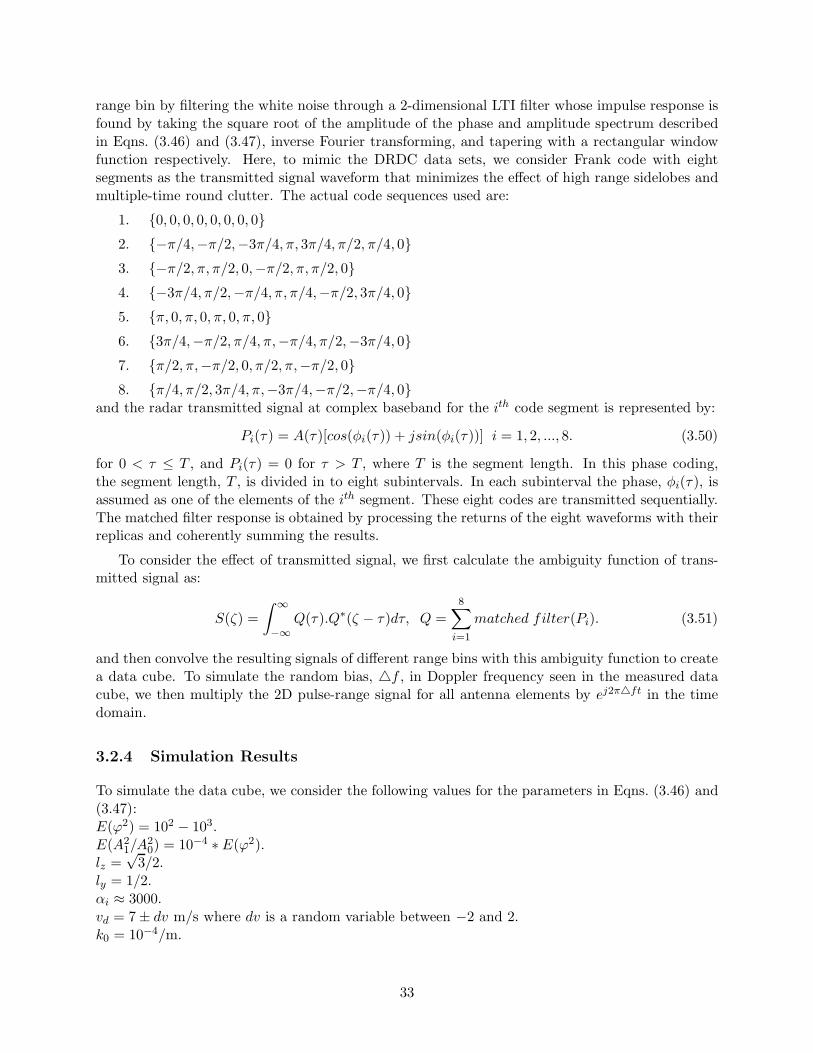
range bin by filtering the white noise through a 2-dimensional LTI filter whose impulse response isfound by taking the square root of the amplitude of the phase and amplitude spectrum describedin Eqns. (3.46) and (3.47), inverse Fourier transforming, and tapering with a rectangular windowfunction respectively. Here, to mimic the DRDC data sets, we consider Frank code with eightsegments as the transmitted signal waveform that minimizes the effect of high range sidelobes andmultiple-time round clutter. The actual code sequences used are:
1. {0, 0, 0, 0, 0, 0, 0, 0}2. {−π/4,−π/2,−3π/4, π, 3π/4, π/2, π/4, 0}3. {−π/2, π, π/2, 0,−π/2, π, π/2, 0}4. {−3π/4, π/2,−π/4, π, π/4,−π/2, 3π/4, 0}5. {π, 0, π, 0, π, 0, π, 0}6. {3π/4,−π/2, π/4, π,−π/4, π/2,−3π/4, 0}7. {π/2, π,−π/2, 0, π/2, π,−π/2, 0}8. {π/4, π/2, 3π/4, π,−3π/4,−π/2,−π/4, 0}
and the radar transmitted signal at complex baseband for the ith code segment is represented by:
Pi(τ) = A(τ)[cos(φi(τ)) + jsin(φi(τ))] i = 1, 2, ..., 8. (3.50)
for 0 < τ ≤ T , and Pi(τ) = 0 for τ > T , where T is the segment length. In this phase coding,the segment length, T , is divided in to eight subintervals. In each subinterval the phase, φi(τ), isassumed as one of the elements of the ith segment. These eight codes are transmitted sequentially.The matched filter response is obtained by processing the returns of the eight waveforms with theirreplicas and coherently summing the results.
To consider the effect of transmitted signal, we first calculate the ambiguity function of trans-mitted signal as:
S(ζ) =
∫ ∞
−∞Q(τ).Q∗(ζ − τ)dτ, Q =
8∑
i=1
matched filter(Pi). (3.51)
and then convolve the resulting signals of different range bins with this ambiguity function to createa data cube. To simulate the random bias, △f , in Doppler frequency seen in the measured datacube, we then multiply the 2D pulse-range signal for all antenna elements by ej2π△ft in the timedomain.
3.2.4 Simulation Results
To simulate the data cube, we consider the following values for the parameters in Eqns. (3.46) and(3.47):E(ϕ2) = 102 − 103.E(A2
1/A20) = 10−4 ∗ E(ϕ2).
lz =√
3/2.ly = 1/2.αi ≈ 3000.vd = 7 ± dv m/s where dv is a random variable between −2 and 2.k0 = 10−4/m.
33
Figure 3.8 shows the shape of Sφ1 and the corresponding autocorrelation when vd = 5. SA1 hasthe same shape as Sφ1 with a different amplitude. The transmitted signal pulse consists of eightphase code segments, each of these segments in turn consists of eight elements, where each elementis 55µs long, and thus each segment is 440µs long. The pulses are emitted every 8ms, thus thecomplete code is emitted every 64ms and the PRF of the data set is 1/64ms = 15.625Hz. Thereare 4096 of these pulses, so the data set is 262.1444 seconds long. The antenna array contains 16antenna elements that are separated by 33.33m from each other. The distance to the first rangebin (z0 in Eqn.(3.49)) is considered 62.75km and the space between range bins (range resolution)is 1.5km. The value of β in Eqn.(3.49) is equal to 103 and the parameter △f , which shows therandom bias in doppler frequency, is considered as a random variable between −0.4 and 0.4. Also,the amplitude of the simulated signal is multiplied by 5×10⁶ to have the same scale as the measuredsignal.
Figures 3.9 and 3.10 show the real and imaginary part of the simulated signal for the range bins34 and 12 when E(ϕ2) is a random variable in the range of 1 ∼ 2×10² and 2 ∼ 3×10² respectively.The corresponding angle-doppler plot of these signals are shown in Fig. 3.11. Figures 3.12, 3.13and 3.14 shows the same results for measured signals. By comparing these results, one can see thatthe simulated signals follow the measured signals with remarkable accuracy. Figures 3.15 and 3.16show the Doppler-range plot of the simulated and measured signals respectively. As the figuresshow, the power of measured signal in frequency domain goes to zero faster than the simulatedsignal. This condition is shown clearly in Fig. 3.17 where the results are shown for a specific rangebin.
3.2.5 Summary
This section presented a core contribution of the work undertaken in this project. A new model ofradio wave propagation in ionosphere plasma density irregularities has been developed. This modelassumes an anisotropic ionospheric plasma that is inhomogeneous in the vertical direction. Inthis model we consider only the first-order phase and amplitude perturbation due to irregularitiesin the ionosphere to model the phase and amplitude power spectrum of the signal. The twodimensional (array element-pulse) signal for each range bin is then created by filtering the whitenoise through a 2-dimensional LTI filter whose impulse response is found by taking the square rootof the amplitude of the phase and amplitude spectrum, inverse fourier transforming and taperingwith a rectangular window function respectively. To consider the effect of the transmitted signal,the ambiguity function of the transmitted signal is convolved with the resulting signals of differentrange bins to make a data cube. To show the accuracy of this method, some simulation resultshas been demonstrated in this report. Comparing these simulated results with measured signalsshows that the simulation results follow the measured signals with remarkable accuracy. The onlyproblem in these results is that the power of the measured signal in frequency domain goes to zerofaster than its simulated counterpart; this issue must must be solved as a future work. In addition,clearly this model is has been tested with data from only a single radar. The general applicabilityof this approach to other ionospheric scenarios is an open question.
34

Figure 3.8: (a) Phase power spectrum and (b) autocorrelation function of the signal.
Figure 3.9: (a) Real and (b) imaginary part of the simulated signal for the range bin 34 when E(ϕ2)is a random value between 1 × 10² and 2 × 10² .
35

Figure 3.10: (a) Real and (b) imaginary part of simulated signal for the range bin 12 when E(ϕ2)is a random value between 2 × 10² and 3 × 10²
.
Figure 3.11: Angle-doppler plot of the simulated signal (a) for the range bins 34 and (b) 12.
36
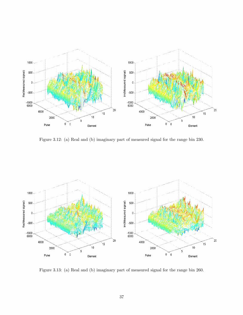
Figure 3.12: (a) Real and (b) imaginary part of measured signal for the range bin 230.
Figure 3.13: (a) Real and (b) imaginary part of measured signal for the range bin 260.
37

Figure 3.14: Angle-doppler plot of the measured signal (a) for the range bins 230 and (b) 260.
Range Doppler power plot (in dB) for element number 13
Doppler in Hz
Ra
ng
e n
um
be
r
−0.5 0 0.50
5
10
15
20
25
30
35
70
75
80
85
90
95
100
105
Doppler in Hz
Ra
ng
e n
um
be
r
Range Doppler power plot (in dB) for element number 6
−0.8 −0.6 −0.4 −0.2 0 0.2 0.4 0.6 0.80
10
20
30
40
50
70
75
80
85
90
95
100
105
Figure 3.15: Doppler-range plot of the simulated signal (a) for antenna element 13 when E(ϕ2) is inthe range of (1 ∼ 2)×102 and (b) for antenna element 6 when E(ϕ2) is in the range of (2 ∼ 3)×102.
38

Doppler in Hz
Ra
ng
e n
um
be
r
Range Doppler power plot (in dB) for element number 6
−0.8 −0.6 −0.4 −0.2 0 0.2 0.4 0.6 0.8
200
210
220
230
240
250
260
75
80
85
90
95
100
105
110
Figure 3.16: Doppler-range plot of the measured signal (a) for antenna element 6.
−8 −6 −4 −2 0 2 4 6 820
30
40
50
60
70
80
90
100
110
Doppler in Hz
po
we
r (in
dB
)
−8 −6 −4 −2 0 2 4 6 820
30
40
50
60
70
80
90
100
110
Doppler in Hz
po
we
r (in
dB
)
Figure 3.17: Doppler plot of the (a) simulated signal of range bin 12 and antenna element 6 and(b) measured signal of range bin 230 and antenna element 6 .
39

Chapter 4
Space-Time Adaptive Processing ofIonospheric Clutter
The central goal of this project is the development of practical space-time adaptive processingschemes for HFSWR radar systems. In a Chapter 2 we had reported on preliminary results ofusing spatial adaptive processing in conjunction with the data set provided by DRDC so far. Inthat report it was suggested that the most important issue with the available data is (a) the non-stationarity of the clutter and (b) the lack of secondary data to estimate the space-time covariancematrix. In this regard, of special interest are adaptive schemes that address clutter non-homogeneityand algorithms with fewer degrees of freedom. Examples of such algorithms are the Joint DomainLocalized (JDL) algorithm [10], the direct data domain (D3) algorithm [48] and the combinationof the two into the hybrid algorithm [7]. Other algorithms of interest are the parametric adaptivematched filter (PAMF) [49]. The hybrid and PAMF algorithms were designed specifically for non-homogeneous clutter. One should emphasize that this list is a starting point for our efforts indeveloping adaptive processing for HFSWR.
In this section we present the results of our preliminary work in applying the JDL algorithm tothe HFSWR data set. However, we first revisit the results provided in Chapter 2 where the issueof oversampling was ignored. It was brought to our attention that the sampling rate used in thedata set is 4× the bandwidth of the transmitted signal, i.e., the data from one sample to the nextis highly correlated. Here we present the results having accounted for this oversampling, but onlyusing every fourth available range sample to estimate the required interference covariance matrices.As we will see, and as expected, this has a significant impact on the achievable performance.
Having reviewed algorithms already available in the literature, we present here the Fast FullyAdaptive (FFA) algorithm tailored for the specific characteristics of the Cape Race data set providedby DRDC. This data set is characterized by an extremely large number of degrees of freedom (4096pulses, 16 channels) coupled with extremely limited training data (only approximately 80 rangebins with ionospheric clutter). This algorithm is a significant advance over previously available
schemes and represents the second major contribution of this project.
40

Broadside
φ
x
d
Figure 4.1: A linear array of point sensors .
4.1 Joint Domain Localized Processing
Consider an equispaced linear array of N isotropic, point sensors receiving an incident plane wave,
as shown in Figure 4.1. Each channel receives M data samples corresponding to the M pulses in
a CPI. Therefore, for each range bin, the received data is a length MN vector x whose entries
numbered mN to [(m + 1)N − 1] correspond to the returns at the N elements from pulse number
m,m = 0, 1, . . . ,M−1. The data vector is a sum of the contributions from the external interference
sources, the thermal noise and possibly a target, i.e.
x = ξs + c + n, (4.1)
where s represents the signal, c the vector of interference sources and n the thermal noise. ξ is the
target amplitude and is zero in range cells without a target.
The term s in Eqn. (4.1) is the space-time steering vector corresponding to a target at angle φt
and Doppler frequency ft. This steering vector can be written in terms of a spatial steering vector
a(φt) and a temporal steering vector b(ft) [44].
s = b(ft) ⊗ a(φt), (4.2)
a(φt) =[1 ej2πfs ej(2)2πfs . . . ej(N−1)2πfs
]T, (4.3)
b(ft) =[1 ej2πft/fR ej(2)2πft/fR . . . ej(M−1)2πft/fR
]T, (4.4)
fs =d
λsinφt, (4.5)
where ⊗ represents the Kronecker product of two vectors, fs the normalized spatial frequency, λ
the wavelength of operation and fR represents the pulse repetition frequency (PRF).
The spatial steering vector a(φ) is the magnitude and phase taper received at the N elements
of the array due to a calibrated far field source at angle φ. Due to electromagnetic reciprocity, to
transmit in the direction φ the elements of the array must be excited with the conjugates of the
41

steering vector, i.e. the conjugates of the steering vector maximize the response in the direction
φ. Transformation of spatial data to the angle domain, at angle φ, therefore requires an inner
product with the corresponding spatial steering vector. Similarly, the temporal steering b(f)
vector corresponding to a Doppler frequency f is the magnitude and phase taper measured at an
individual element for the M pulses in a CPI. An inner product with the corresponding temporal
steering vector transforms time domain data to the Doppler domain. The angle-Doppler response
of the data vector x at angle φ and Doppler f is therefore given by
x(φ, f) = [b(f) ⊗ a(φ)]H x, (4.6)
where the tilde ( ˜ ) above the scalar x signifies the transform domain. Choosing a set of spatial
and temporal steering vectors generates a corresponding vector of angle-Doppler domain data.
Equations (4.2)-(4.4) show that the spatial and temporal steering vectors are identical to the
Fourier coefficients. Based on this observation, the transformation to the angle-Doppler domain
can be simplified under two conditions.
1. If a set of angles are chosen such that ( dλ sinφ) is spaced by 1/N and a set of Doppler
frequencies are chosen such that (f/fR) is spaced by 1/M , the transformation to the angle-
Doppler domain is equivalent to the 2D DFT.
2. If the look angle φt corresponds to one these angles and the look Doppler ft corresponds
to one of these Dopplers, the 2-D DFT transforms the target data to a single point in the
angle-Doppler domain, i.e. the signal is localized.
The second condition is based on the orthogonality of the DFT. This simplification is possible only
in the case of the ideal array of Fig. 4.1.
The JDL algorithm as developed in [9] assumes both these conditions are met. A Local Pro-
cessing Region (LPR), as shown in Fig. 4.2, is formed about the signal point and interference is
suppressed in this region only. The LPR covers ηa angle bins and ηd Doppler bins. The choice of ηa
and ηd is independent of N and M , i.e. the transformation to the angle-Doppler domain decouples
the number of adaptive degrees of freedom from the size of the data cube. The covariance matrix
corresponding to this LPR is estimated using secondary data from neighboring range cells. The
adaptive weights are calculated by
w = R−1s, (4.7)
42

Local Processing Region
Doppler bins
Angle bins
Signal
Figure 4.2: Localized processing regions in Joint Domain Localized processing.
where R is the estimated covariance matrix corresponding to the LPR of interest. The number of
adaptive unknowns is equal to ηaηd. Because of the fewer unknowns involved, the covariance matrix
can be accurately estimated from a limited number of secondary data samples. s is the steering
vector for the adaptive process. This vector must not be confused with either the spatial steering
vector (a) or the temporal steering vector (b) of Eqns. (2.4)-(2.5). s is the space-time vector of
equation (4.2) transformed to the angle-Doppler domain and is given by the length ηaηd vector
s = [0, 0, · · · , 0, 1, 0, · · · , 0, 0]T . (4.8)
It must be emphasized that this simple form of the steering vector is valid only because it is the
space-time steering vector transformed to the angle-Doppler domain using the same transformation
as used for the data. The adaptive weights are used to find a statistic, such as the MSMI statistic,
for detection by hypothesis testing.
The JDL algorithm described above can be generalized as follows: Fig. 4.2 shows that data from
the LPR of interest is used for the adaptation process. Eqn. (4.6) indicates that the transformation
from the space-time domain to the angle-Doppler domain is, in effect, an inner product with a
space-time steering vector. This argument holds true for ideal linear arrays and physical arrays.
Mathematically, the relevant transformation is therefore a pre-multiplication with a transformation
matrix. For example, if the LPR covers 3 angle bins (φ−1, φ0, φ1; ηa = 3) and 3 Doppler bins
43
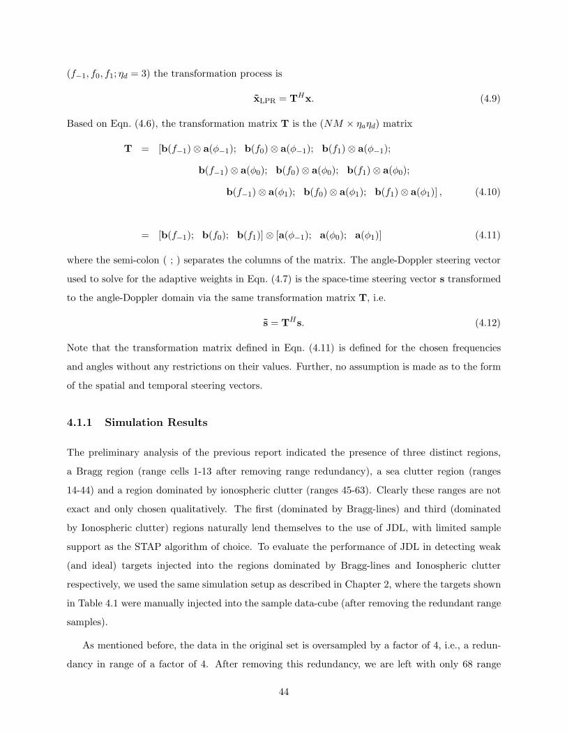
(f−1, f0, f1; ηd = 3) the transformation process is
xLPR = THx. (4.9)
Based on Eqn. (4.6), the transformation matrix T is the (NM × ηaηd) matrix
T = [b(f−1) ⊗ a(φ−1); b(f0) ⊗ a(φ−1); b(f1) ⊗ a(φ−1);
b(f−1) ⊗ a(φ0); b(f0) ⊗ a(φ0); b(f1) ⊗ a(φ0);
b(f−1) ⊗ a(φ1); b(f0) ⊗ a(φ1); b(f1) ⊗ a(φ1)] , (4.10)
= [b(f−1); b(f0); b(f1)] ⊗ [a(φ−1); a(φ0); a(φ1)] (4.11)
where the semi-colon ( ; ) separates the columns of the matrix. The angle-Doppler steering vector
used to solve for the adaptive weights in Eqn. (4.7) is the space-time steering vector s transformed
to the angle-Doppler domain via the same transformation matrix T, i.e.
s = THs. (4.12)
Note that the transformation matrix defined in Eqn. (4.11) is defined for the chosen frequencies
and angles without any restrictions on their values. Further, no assumption is made as to the form
of the spatial and temporal steering vectors.
4.1.1 Simulation Results
The preliminary analysis of the previous report indicated the presence of three distinct regions,
a Bragg region (range cells 1-13 after removing range redundancy), a sea clutter region (ranges
14-44) and a region dominated by ionospheric clutter (ranges 45-63). Clearly these ranges are not
exact and only chosen qualitatively. The first (dominated by Bragg-lines) and third (dominated
by Ionospheric clutter) regions naturally lend themselves to the use of JDL, with limited sample
support as the STAP algorithm of choice. To evaluate the performance of JDL in detecting weak
(and ideal) targets injected into the regions dominated by Bragg-lines and Ionospheric clutter
respectively, we used the same simulation setup as described in Chapter 2, where the targets shown
in Table 4.1 were manually injected into the sample data-cube (after removing the redundant range
samples).
As mentioned before, the data in the original set is oversampled by a factor of 4, i.e., a redun-
dancy in range of a factor of 4. After removing this redundancy, we are left with only 68 range
44

Table 4.1: Target Characteristics
Target Number Amplitude Range Number Angle Doppler
1 5 7 (within Bragg region) 35o 0.18Hz
2 5 54 (within Ionospheric clutter region) 35o 0.18Hz
cells. For the region dominated by the Bragg-line we have, for each look range, only 11 range cells
that correctly reflect the interference statistics in the Bragg line region and can be used as sec-
ondary range cells in estimating the covariance matrix. Similarly in the ionospheric clutter region
only 17 independent ranges are available to estimate the clutter covariance matrix. Hence, in our
results instead of selecting ηaηd ranges on either side of a specific look range as secondary range
samples, we calculated the interference covariance matrix using all the ranges belonging to the
region of interest (Bragg-line or Ionospheric region) except for the corresponding look range which
was excluded from the covariance estimation procedure. Note that we did not use any spatial or
temporal tapers for the purposes of this simulation, although the incorporation of such tapers into
the transformation matrix could lead to improved performance.
Given the constraints on the available secondary data samples, one can only have 6 degrees of
freedom ( ηaηd < 6) in the region dominated by Bragg lines; similarly we can have only 9 DOF in
the ionospheric clutter region (ηaηd < 9) . However, given the availability of redundant data, in
our simulations we chose (ηaηd) = (3,3) , (3,5) ,and (3,7) for the Bragg-line dominated region , and
(ηaηd) = (3,3) ,(3,5), and (3,7) for the Ionospheric clutter dominated region. Even though several
of the selected (ηaηd) pairs do not theoretically lead to acceptable results (since their product is
greater than the number of available independent training ranges), we chose them so as to verify
this using simulation.
Angle Doppler Spacing
The work of [10] removed the spacing constraint between angle and Doppler bins that had been
placed by the original JDL work of [9]. However, there is no available theory to determine an
optimal spacing between angle or Doppler bins. The only recourse we have is to use simulations
(another reason to implement a data model). The first set of results we present estimate the
performance of the JDL algorithm as a function of angle and Doppler spacing.
45

Figure 4.3: ∆MSMI versus angle and Doppler spacing (ηa = ηd = 3). Ionospheric clutter region.
Figure 4.3 plots (∆MSMI), the difference between the MSMI statistic at the target range cell
and the next largest MSMI statistic (i.e., the largest false alarm statistic), as a function of angle and
Doppler spacing, for ηa = 3 and ηd = 3. ∆MSMI, therefore, measures how easy it is to distinguish
the target from the background clutter. The figure illustrates that the JDL algorithm is fairly
sensitive to angle and Doppler spacing with the difference in statistic varying by as much as 15dB.
There are some regions where the ∆MSMI is set to zero since its true value is negative, i.e., the
target is buried in clutter. However, the majority of the choices of spacing provide a ∆MSMI larger
than 6dB. As we will see, when the target is in the Bragg region, the JDL algorithm appears to
fail for most choices of angle and Doppler spacings.
Figure 4.4 recreates Figure 4.3 for the case where the target is within the Bragg lines. As can
be seen, the target is almost never detected and the JDL method fails. Furthermore, the ∆MSMI
is positive for only a few choices of angle and Doppler spacing.
Figure 4.5 and Figure 4.6 show that similar comments can be made for the case of ηa = 3
and ηd = 5. Interestingly, in this case the spacing that gives the greatest target discrimination is
significantly smaller than in the case of ηa = 3 and ηd = 3. Obtaining an optimum spacing is one
that will require many more data sets and simulation before a rule of thumb can be obtained.
46

Figure 4.4: ∆MSMI versus angle and Doppler spacing (ηa = ηd = 3). Bragg region.
Figure 4.5: ∆MSMI versus angle and Doppler spacing (ηa = 3, ηd = 5). Ionospheric clutter region.
47

Figure 4.6: ∆MSMI versus angle and Doppler spacing (ηa = 3, ηd = 5). Bragg region.
Target Detection Using JDL
Figure 4.7 and Figure 4.8 plot the MSMI statistic versus range cell number for the optimal spacings
found in the previous plots for the case of (ηa = ηd = 3). In the ionospheric clutter region,
this configuration is adequate to clearly isolate the target from the surrounding clutter. For the
amplitude given in Table 1, the MSMI statistic provides a discrimination of 13 + dB.
Figure 4.8 plots the MSMI statistic when the same target is placed in the region dominated by
the Bragg lines. In this case, the target cannot be identified with minimal discrimination between
target and clutter. This is because only 12 range cells are available to estimate the 9×9 covariance
matrix resulting in an extremely poor covariance estimate.
Figure 4.9 plots the MSMI statistic versus range with ηa = 3, ηd = 7 in the region dominated by
the ionospheric clutter. The improved detection over Figure 4.7 is clearly visible. Note that in this
example we used only 17 range cells to estimate the interference covariance matrix. The covariance
matrix is therefore singular. However, here the matrix inverse is replaced by the min-norm solution
to the under-determined system of equations available. The min-norm solution finds, in the family
of possible solutions, the vector with minimum norm. Note that this indicates that the rank of the
interference is low and increasing the number of degrees of freedom improves target discrimination.
However, one should be cautious because the target is an ideal target and the adaptive process
48

Figure 4.7: MSMI statistic (in dB) versus the range cell number for (ηa = ηd = 3). Ionospheric
clutter region.
does not include any target mis-match.
Figure 4.10 plots the MSMI statistic versus range for the case of ηa = 3, ηd = 7, i.e., with
21 degrees of freedom, when the target is in the region dominated by the Bragg lines. Again the
covariance matrix is singular and requires the min-norm solution. The low rank of the interference
again allows for significant interference suppression with larger numbers of DOF. The target is
clearly seen. This figure illustrates the potential of using JDL in the Bragg region as well.
We should mention that we have attempted to obtain MSMI results for the case where we use
all available data without removing the redundancy. As with the earlier report, these plots provide
highly optimistic results and are a matter of further investigation. For example, with ηa = 3
and ηd = 7 in the ionospheric region, when using all range cells we get the results as shown in
Figure 4.11. The target discrimination is beyond our expectations. This may be due to,
1. the fact by using both spatial and Doppler degrees of freedom we are exploiting the very
large number of coherent pulse intervals in addition to the 7 Doppler DOF (unlike when
using adaptive processing in the spatial dimension only),
2. the large number of range cells (17 × 4 = 68) used to estimate the 21 × 21 covariance matrix.
The data, therefore, though correlated appears to have sufficient independence to provide
49

Figure 4.8: MSMI statistic (in dB) versus the range cell number for (ηa = ηd = 3). Bragg region.
Figure 4.9: MSMI statistic (in dB) versus the range cell number for (ηa = 3, ηd = 7). Ionospheric
clutter region.
50

Figure 4.10: MSMI statistic (in dB) versus the range cell number for (ηa = 3, ηd = 7). Bragg
region.
improved estimates of the angle-Doppler covariance matrix.
4.1.2 Discussion
When using ideal targets, the JDL algorithm provides excellent results in identifying targets that
could not be identified by non-adaptive processing. In fact, JDL processing appears to perform
better than the spatial-only case presented earlier. One essential drawback of JDL, though, is
its heavy reliance on the homogeneity of the data used to estimate the interference covariance
matrix. Unfortunately in practice it is seldom the case that the secondary data is homogeneous.
The presence of discrete interferers for example can compromise the homogeneity of the secondary
data and as a result lead to an inaccurate estimate of the interference covariance matrix, leading
to a large degradation in the performance of JDL.
One must therefore use non-homogeneity detectors (NHD) to filter non-homogeneous range
cells [6]. Alternatively, methods that do not rely on the computation of an estimate of the interfer-
ence covariance matrix can be used to avoid the problem of inhomogeneous secondary data samples,
altogether. Such methods include the direct data domain (D3) [48] and the hybrid approach [7]
which focus exclusive (the D3 algorithm) or predominantly on the range cell of interest (the hy-
51

Figure 4.11: MSMI statistic (in dB) versus (in dB) versus the range cell number for (ηa = 3, ηd = 7).
Using all range cells in ionospheric clutter region.
brid approach). In the next sections we investigate both these algorithms. It is also interesting
to mention that JDL is not the only member of the low computation load family of STAP algo-
rithms. Several other low computation methods have also been developed and address the issue of
computation load in innovative and diverse methods. Some of the most popular low computation
algorithms, other than JDL, include the parametric adaptive matched filter (PAMF) [49], and the
multistage Weiner filter (MWF) [50]. In the next section we will investigate the relevance of the
PAMF algorithm to our work.
Our results so far lead to a fundamental question: how do we measure success effectively in
an adaptive process, i.e., how do we compare algorithms? There are two traditional approaches
to estimating performance, (i) using the gain of the adapted pattern with the assumption that an
array with higher gain has better performance and (ii) injecting targets and then measuring target
discrimination as we have done above. This second approach is particularly popular when using
measured data as we are doing in this project. However, there are serious issues with both these
approaches.
The use of an adapted pattern to measure performance is valid only in homogeneous scenarios
with relatively little structured interference. This is because without knowing a priori where the
interference is located a pattern with lower array gain might be better in terms of interference
52

suppression. A related concept, of measuring the output signal-to-interference-plus-noise ratio
(SINR) is valid in homogeneous scenarios only. The output SINR is defined as
SINR =
∣∣wHs∣∣2
wHRw, (4.13)
where w is the weight vector, R is the interference covariance matrix and v is the target space-time
steering vector. Furthermore, the weight vector w = R−1v. However, the fundamental assumption
is that the covariance matrix R is representative of the interference in the range cell under test. In
STAP, this covariance matrix is obtained using secondary data, i.e., we are assuming the secondary
data is representative of the statistics of the interference in the range cell under test. The other
approach is to inject a target and determine the discrimination between the output statistic at the
target range cell versus surrounding range cells. This is the approach taken above and has been
taken in most of the research into the Multi-Channel Airborne Radar Measurements (MCARM)
data set - see [10] for one example. However, this approach is only as useful as the model for a
target is valid. In this report we have used a straightforward target model, but have ignored such
issues as the redundancy in the data sampling process and hence the spread of the target as a
function of range.
In summary, the JDL algorithm adaptive processes angle-Doppler data, i.e., after transfor-
mation from the space-time to the angle-Doppler domain. Adaptive processing focuses on a small
localized processing region (LPR) within the angle-Doppler domain; specifically, the JDL algorithm
adaptively processes ηa angle bins and ηd Doppler bins, i.e., only ηaηd adaptive weights are used.
Considering that the usual values of ηa and ηd are between 3 and 5, the resulting computation load
reduces from the solution of a NM × NM matrix to that of a ηaηd × ηaηd matrix.
The main drawback of using JDL is its inherent dependance on the homogeneity of the secondary
data. Unfortunately the highly nonhomogeneous and non-stationary nature of the ionospheric
clutter as well as the limited availability of secondary data are all factors that are capable of
seriously degrading the performance of JDL in the ionospheric clutter region.
In the following sections, we use the hybrid algorithm to achieve suppression of both non-
homogeneous and homogeneous components of the clutter. The hybrid algorithm builds on the
JDL algorithm using an adaptive transform from the space-time to the angle-Doppler domain.
Specifically, the adaptive transform uses direct data domain (D3) processing; adaptive processing
without requiring secondary data. D3 processing was first developed in [48] for the spatial-only
case and then extended to space-time processing in [7]. The latest work in this area [51] develops
53

an alternative approach that is significantly more stable computationally.
The D3 algorithm processes each range cell individually and is thus immune to any uncorrelated
interference present at a certain range cell. However, since the D3 algorithm completely ignores
any statistical information that might be derived from the secondary data about the correlated
part of the interference present in the target range, it is not as effective as the JDL algorithm in
suppressing correlated interference. This deficiency is accounted for in the hybrid algorithm [7]
which combines the advantages of both the D3 and JDL algorithms to suppress both coherent and
incoherent interference present in the target range. We will describe the hybrid algorithm in a
subsequent section.
The hybrid algorithm has some significant advantages in that it can address both homogeneous
and non-homogeneous components of clutter. However, it does have some drawbacks. First, the
hybrid algorithm is fairly computationally expensive. Also, in the context of ionospheric clutter,
the clutter non-homogeneities are not localized which is the ideal scenario for the D3 algorithm.
Another powerful algorithm that was designed to show both improved computational speed
and high accuracy as well as a certain degree of robustness towards non-homogeneous data, is the
parametric adaptive matched filter (PAMF) algorithm [49]. The PAMF approach uses linear filter
theory to estimate the inverse of the covariance matrix in a computationally efficient manner and
significantly reduced required sample support to obtain the output statistic. The only drawback of
the PAMF approach is that there is no clear way to integrate D3 processing for non-homogeneous
clutter.
The second problem in the previous report is one of modeling the target. In the previous work,
the JDL algorithm was used to detect a single point target injected into a single range bin. This is
clearly a idealized situation; in the real world, a target is distributed over range bins. In this report
we present results of using a real (measured) target signal extracted from a noise-limited data set
provided by DRDC.
In the next sections, after describing the D3, hybrid, and PAMF algorithms, we will present
the simulation results of applying these algorithms to both ideal and real targets int the Bragg and
ionospheric clutter region. We will also follow up on JDL by presenting simulation results using
JDL on real targets.
54

4.2 The Direct Data Domain Algorithm
The D3 algorithm, developed in [7] and improved upon in [51], is a purely non-statistical algorithm
which does all its processing using only the current look range without relying on the neighboring
ranges to extract an estimate of the error covariance matrix. As a result the D3 algorithm is immune
to both clutter non-homogeneities in the secondary data and target-like, discrete, interference
sources within the primary range cell. The discrete interference may be occupy multiple angle and
Doppler bins. This scenario is more relevant to us since the ionospheric clutter, with its highly
nonhomogeneous nature, may be characterized as a source of high power discrete interference spread
over numerous range cells leading to a contamination of the homogeneity of the secondary data.
We begin with a brief description of how the improved D3 algorithm of [51] works. Assuming
the usual N element, M pulse scenario we form the N × M data matrix X at range cell r:
X = ξV + C + N, (4.14)
V = a(ϕt) ⊗ bT (ft), (4.15)
a(ϕt) = [ 1 zs · · · z(N−1)s ]
T, (4.16)
b(ft) = [ 1 zt · · · z(M−1)t ]
T, (4.17)
zs = ei2π(d/λ) sin(ϕt), (4.18)
zt = ei2π(ft/fR), (4.19)
where ξ is the target amplitude, a(ϕt) and b(ft) are the target spatial and temporal steering vectors
respectively, at azimuth ϕt and Doppler ft , and C and N are the clutter and noise space-time
matrices respectively.
Next we form the temporal residual matrix At as follows,
At = X(0 : M − 2, 0 : N − 1) − z−1t X(1 : M − 1, 0 : N − 1) (4.20)
where we used MATLABr notation to specify the two submatrices used in the above matrix
difference. We can therefore write the (i, j)th term of the matrix At as,
At(i, j) = X(i, j) − z−1t X(i, j + 1), i = 0, .., N − 1 j = 1, ...,M − 2 (4.21)
If X were to contain a target, then the above procedure yields a residual matrix A free from any
target terms.Ideally the entries of matrix At carry interference only terms, but due to possible beam
55

mis-match, some negligibly small residual target information may still be present in the entries of
At.
We will next make use of the following scalar terms in an attempt to null the discrete interference,
Gwt =∣∣∣bH
(0:M−2)wt
∣∣∣2
(4.22)
Iwt = ‖A∗t wt‖2 (4.23)
SINRresidual ∝ Gwt
Iwt=
wHt b(0:M−2)b
H(0:M−2)wt
wHt AT
t A∗t wt
(4.24)
where Gwt represents the target signal power after temporal filtering with the weight vector wt,
and Iwt represents the residual interference power after temporal filtering. As a result the residual
SINR can be defined as the ratio of these two terms, and our task is to select an optimal temporal
filter wt that maximizes the above SINR.
wtopt = arg max{wt}
(SINRresidual) (4.25)
The solution to the above optimization problem can be shown to be,
wtopt =(AT
t A∗t
)−1b(0:M−2) (4.26)
if(AT
t A∗t
)−1exists. If this matrix inverse does not exist, the solution is the eigenvector corre-
sponding to the large generalized eigenvalue of the matrix pair(AT
t A∗t ,b(0:M−2)b
H(0:M−2)
).
Optimal D3 spatial weights can be obtained in a similar manner. Define As as the residual
spatial interference matrix,
As =(X(0 : M − 1, 0 : N − 2) − z−1
t X(0 : M − 1, 1 : N − 1))T
(4.27)
whose (i, j)th term is given by,
As(i, j) = X(j, i) − z−1t X(j + 1, i) (4.28)
Next define the target signal power, residual interference power, and SINR after spatial filtering as,
Gws =∣∣∣aH
(0:N−2)ws
∣∣∣2
(4.29)
Iws = ‖A∗sws‖2 (4.30)
SINRresidual ∝Gws
Iws=
wHs a(0:N−2)a
H(0:N−2)ws
wHs AT
s A∗sws
(4.31)
We can therefore obtain the optimal spatial weights by maximizing the above SINR which yields,
wsopt =(AT
s A∗s
)−1a(0:N−2). (4.32)
56

We then obtain the optimal spatio-temporal set of weights, w, as
w =
wtopt
0
⊗
wsopt
0
. (4.33)
The 0 terms represent the lost spatial and lost temporal degrees of freedom.
Because the algorithm does not require any secondary data, the D3 is capable of suppressing
any uncorrelated interference present in the target range. However since D3 is a nonstatistical
algorithm it suffers from poor performance when correlated (homogeneous) interference is present
in the target’s range. One other disadvantage of the D3 algorithm is that it requires the computation
of the inverse of an (M − 1)× (M − 1) matrix which can be quite a daunting task for large number
of pulses. In the DRDC data sets, M = 4096, making the matrix in question singular. Even finding
the generalized eigenvalues becomes difficult since the algorithms involved become unstable.
In the following section we will describe the hybrid algorithm which uses D3 as a first stage
to eliminate (null out) discrete interference sources contaminating the target range, then uses the
JDL algorithm on this ’purified’ data to suppress the correlated interference.
4.3 The Hybrid Algorithm
The hybrid algorithm was developed in [7] for airborne radar applications. It is a two stage
algorithm whose building blocks are the D3 and JDL algorithms. The hybrid algorithm can be
summarized in the following steps:
1. Form a Localized Processing Region (LPR) by choosing a set of ηa angle bins centered at the
look angle, and ηd Doppler bins centered at the look Doppler.
2. For each angle-Doppler bin,(φ−i, f−j) within the LPR form the corresponding space-time
steering vector and use the D3 algorithm to obtain the adaptive weight vector w(φ−i, f−j)
that transforms the look range from the space-time domain to the angle-Doppler.
3. After looping over all the LPR bins form the adaptive transformation matrix TD3. For
example, for 3 angle and 3 Doppler bins TD3 is given by,
57

TD3 = [w(φ−1, f−1) w(φ0, f−1) w(φ1, f−1)
w(φ−1, f0) w(φ0, f0) w(φ1, f0)
w(φ−1, f1) w(φ0, f1) w(φ1, f1)]
(4.34)
4. Transform the target range space-time vector and all the secondary ranges to the angle-
Doppler domain via the transformation matrix TD3.
5. Apply the JDL algorithm to the transformed domain to obtain the optimal weight vector
given by,
whybrid = R−1v (4.35)
6. Compute the CFAR MSMI test statistic as follows,
MSMI =
∣∣∣wHhybrid
∧x∣∣∣2
wHhybrid
∧v
(4.36)
Thus the hybrid algorithm suppresses any discrete interference that might be present at the
target range in its first, D3 stage, effectively transforming the datacube to the angle-Doppler do-
main. It then nulls the correlated interference by computing a weight vector derived from the
estimate of the error covariance matrix in the transformed domain. The main drawback of the
hybrid algorithm is its large computational time, since it has to apply the D3 algorithm for each of
the ηaηd angle-Doppler bins of the LPR.
4.4 The Parametric Adaptive Matched Filtering Algorithm
The PAMF algorithm was developed in [49]. The primary idea behind this algorithm is the use of
linear estimation theory to obtain an estimate of the inverse of the error covariance matrix which
can be computed much more rapidly than in the conventional AMF method. PAMF is based
on the block-LDL decomposition of the covariance matrix, R, where the non-zero block elements
of the lower triangular block matrix, L, resulting from the decomposition, corresponding to each
block row p, are the coefficients of a multichannel autoregressive process of order p, whose error
covariance matrix is the p-th block matrix of the block diagonal matrix D resulting from the LDL
decomposition of R. Since R is not known a priori the coefficients of L and D must be approximated
by assuming a p-th order multichannel AR process to be the underlying process and using an
58
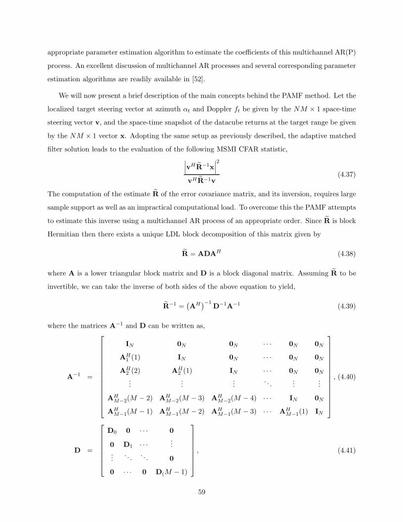
appropriate parameter estimation algorithm to estimate the coefficients of this multichannel AR(P)
process. An excellent discussion of multichannel AR processes and several corresponding parameter
estimation algorithms are readily available in [52].
We will now present a brief description of the main concepts behind the PAMF method. Let the
localized target steering vector at azimuth αt and Doppler ft be given by the NM × 1 space-time
steering vector v, and the space-time snapshot of the datacube returns at the target range be given
by the NM × 1 vector x. Adopting the same setup as previously described, the adaptive matched
filter solution leads to the evaluation of the following MSMI CFAR statistic,
∣∣∣vHR−1x
∣∣∣2
vHR−1v(4.37)
The computation of the estimate R of the error covariance matrix, and its inversion, requires large
sample support as well as an impractical computational load. To overcome this the PAMF attempts
to estimate this inverse using a multichannel AR process of an appropriate order. Since R is block
Hermitian then there exists a unique LDL block decomposition of this matrix given by
R = ADAH (4.38)
where A is a lower triangular block matrix and D is a block diagonal matrix. Assuming R to be
invertible, we can take the inverse of both sides of the above equation to yield,
R−1 =(AH
)−1D−1A−1 (4.39)
where the matrices A−1 and D can be written as,
A−1 =
IN 0N 0N · · · 0N 0N
AH1 (1) IN 0N · · · 0N 0N
AH2 (2) AH
2 (1) IN · · · 0N 0N
......
.... . .
......
AHM−2(M − 2) AH
M−2(M − 3) AHM−2(M − 4) · · · IN 0N
AHM−1(M − 1) AH
M−1(M − 2) AHM−1(M − 3) · · · AH
M−1(1) IN
, (4.40)
D =
D0 0 · · · 0
0 D1 · · · ......
. . .. . . 0
0 · · · 0 D(M − 1)
, (4.41)
59

where the N ×N submatrix AHi (j) is the i’th row and (j-i)’th column block elements of matrix A
(i, j = 0, · · · ,M − 1), and are not characterized by any particular structure. Note that the block
diagonal matrices AHi (0) are equal to the N ×N identity matrix. Also the N ×N submatrices Di,
i = 0, · · · ,M − 1), are the block diagonal elements of the matrix D. It was shown in [49] that the
set of matrices {AHm(m),AH
m(m− 1), · · · ,AHm(1)} for m = 0, · · · ,M − 1, are the matrix coefficients
of a m-th order multichannel forward linear predictor for a vector process {x(m)} whose covariance
matrix of the m-th order prediction error vector is given by the m-th block diagonal element Di.
This can be written as,
xm(m) = −m∑
k=1
AHm(k)x(m − k) {m = 0, · · · ,M − 1}
εm(m) = x(m) − xm(m) =m∑
k=0
AHm(k)x(m − k)
E[εm(m)] = Dm
{x(m)} =[
· · · x(0) x(1) . . . x(m) · · · x(M − 1) · · ·]
(4.42)
In the above equation the vector term ǫ is the error vector of the AR(m) process. As can be seen from
the above equation this error vector is the output of the m-th order multichannel moving average
process (MA(m)) whose coefficients are the matrix coefficients of the corresponding multichannel
AR(m) process, and whose input is the vector process {x(m)}.
So far our entire discussion is general and applies to any invertible, block hermitian, matrix
R. The reason we chose x to denote the vector process will be clear after we plug in the LDL
representation of R into the expression for the MSMI statistic.
ΛMF =
∣∣(D−1/2A−1v)H(D−1/2A−1x)∣∣2
(D−1/2A−1v)H(D−1/2A−1v)
=
∣∣(D−1/2u)H(D−1/2ε)∣∣2
(D−1/2u)H(D−1/2u)=
∣∣sHr∣∣2
sHs(4.43)
u = A−1v (4.44)
ε = A−1x (4.45)
s = D−1/2u (4.46)
r = D−1/2ε (4.47)
60
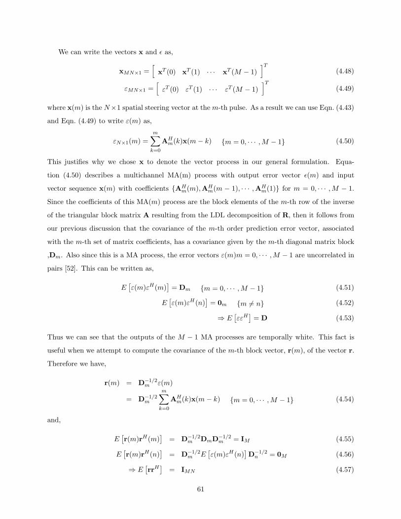
We can write the vectors x and ǫ as,
xMN×1 =[
xT (0) xT (1) · · · xT (M − 1)]T
(4.48)
εMN×1 =[
εT (0) εT (1) · · · εT (M − 1)]T
(4.49)
where x(m) is the N×1 spatial steering vector at the m-th pulse. As a result we can use Eqn. (4.43)
and Eqn. (4.49) to write ε(m) as,
εN×1(m) =
m∑
k=0
AHm(k)x(m − k) {m = 0, · · · ,M − 1} (4.50)
This justifies why we chose x to denote the vector process in our general formulation. Equa-
tion (4.50) describes a multichannel MA(m) process with output error vector ǫ(m) and input
vector sequence x(m) with coefficients {AHm(m),AH
m(m − 1), · · · ,AHm(1)} for m = 0, · · · ,M − 1.
Since the coefficients of this MA(m) process are the block elements of the m-th row of the inverse
of the triangular block matrix A resulting from the LDL decomposition of R, then it follows from
our previous discussion that the covariance of the m-th order prediction error vector, associated
with the m-th set of matrix coefficients, has a covariance given by the m-th diagonal matrix block
,Dm. Also since this is a MA process, the error vectors ε(m)m = 0, · · · ,M − 1 are uncorrelated in
pairs [52]. This can be written as,
E[ε(m)εH(m)
]= Dm {m = 0, · · · ,M − 1} (4.51)
E[ε(m)εH (n)
]= 0m {m 6= n} (4.52)
⇒ E[εεH
]= D (4.53)
Thus we can see that the outputs of the M − 1 MA processes are temporally white. This fact is
useful when we attempt to compute the covariance of the m-th block vector, r(m), of the vector r.
Therefore we have,
r(m) = D−1/2m ε(m)
= D−1/2m
m∑
k=0
AHm(k)x(m − k) {m = 0, · · · ,M − 1} (4.54)
and,
E[r(m)rH(m)
]= D−1/2
m DmD−1/2m = IM (4.55)
E[r(m)rH(n)
]= D−1/2
m E[ε(m)εH (n)
]D−1/2
n = 0M (4.56)
⇒ E[rrH
]= IMN (4.57)
61

Thus the vectors r(m) are both temporally and spatially white. Thus the coefficient matrix A acts
as a temporal whitening filter which is followed by a spatial whitening filter embodied in the matrix
D. The same expressions can be obtained for the vectors u and s.
In order to bypass the computation of the inverse of an estimate of R it suffices to estimate the
coefficient matrix A−1 and residual covariance matrix D, and use them in (Eqn. (4.43)) to directly
compute the MSMI criterion. The first step to achieving this is to select an appropriate AR order
that accurately portrays the underlying statistics. After the order, P , has been selected we can
rewrite the PAMF detection statistic as,
ΛPAMF =
∣∣∣∣M−P−1∑
m=0sH(m)r(m)
∣∣∣∣2
M−P−1∑m=0
sH(m)s(m)
εN×1(m) =
P∑
k=0
AH(k)x(m − k + P ) {m = 0, · · · ,M − P − 1}
r(m) = D−1/2P
P∑
k=0
AH(k)x(m − k + P ) {m = 0, · · · ,M − P − 1}
(4.58)
where the following modifications were administered to the definitions of ǫ and r in order to obtain
this new estimate of the AMF MSMI criterion:
1. retain only the vector sequences for a MA filter of order P ≤ M − 1.
2. Let the MA filtering step be a moving window instead of a block window.
Since A and Dp are unknown they must be estimated via an appropriate multichannel parameter
estimation method. It was shown through theory in [52] and through simulation in [49] that
the best parameter estimation method for STAP is the Least Squares method (also known as
the covariance method). Simulation results in [49] suggest that an order P = 3 (<<< MN)
multichannel AR process is sufficient to accurately model the underlying process for airborne radar
and as a result the computational cost associated with the least squares multichannel parameter
estimation method(which forms the main block of the PAMF algorithm) is significantly lower than
the O((MN)3) load associated with the inversion of estimate of R in the AMF method. The least
62

squares problem can be expressed as follows,
XHr XrA
′ = XHr xr
xrL×N
=[
xTr (M − 1) xT
r (M − 2) · · · xTr (M − L)
]T
Xr(t)L×NP =[
xr(t) xr(t − 1) · · · xr(t − P )]
A′
NP×NP=[
AH(1) AH(2) · · · AH(P )]
(4.59)
where the subscript r denotes the range cell of interest, and L denotes the number of pulses used
in the least square solution. A necessary but insufficient condition for XHr Xr to be nonsingular
is P ≤ L/2. We will set L = ⌊2M/3⌋ in our simulations. Therefore for a nonsingular XHr Xr the
solution to the least square problem is,
A′ =(XH
r Xr
)−1XH
r xr (4.60)
The PAMF method also shows robustness to the presence of discrete interference in the sec-
ondary data [49] and has performance that rivals that of the MF even in the case of limited sample
support. Unfortunately the PAMF method is not CFAR, however simulation results suggest that
for certain PAMF configurations CFAR like behavior does occur [49].
In our simulations we use the least squares parameter estimation method as well as two different
methods for the estimation of the spatial whitening block filter (i.e., the block diagonal elements
of D) namely the residual sample covariance matrix,
Dp(m) =1
K
K∑
k=1
ε(n, k/H0)εH(n, k/H0) {m = 0, · · · ,M − P − 1} (4.61)
and time average sample covariance matrix methods,
Dp =1
(M − P − 1)
M−P−1∑
m=0
Dp(m) (4.62)
In the residual covariance matrix method the average is taken over range cells that do not contain
target residues (thus the H0 conditional hypothesis). In compliance with the Brennan rule it is
assumed that K ≥ 2N . The first method has the advantage of yielding a more CFAR like behavior
while the second method has the advantage of larger detection probability [49]. In the results
section we will provide simulation results of applying the PAMF to detect ideal and real targets
injected in the datacube.
63

4.5 Realistic Target Model
Assuming a point target model has several advantages such as simplicity, localization to a single
range bin, and the eliminating the need to incorporate the ambiguity function into the target model.
Unfortunately ideal targets do not exist in the real world and we must therefore choose a realistic
target model that more accurately portrays what is really happening. So far we have conducted
simulations using ideal point targets localized to exactly one range cell. This resulted in some
rather optimistic results for JDL that were perhaps not totally reflecting of its true performance
in a practical scenario where the ideal target would be replaced by a realistic target spread over
multiple ranges. To account for the spread of real targets in range we used obvious realistic targets
directly extracted from a sample data-square (since only one spatial channel was used) provided to
us by Dr. Riddolls. Figure 4.12 shows a range-Doppler plot of this data-square where the targets
are indicated by arrows. Figure 4.13 shows several superposed cross-sections of the range-Doppler
Figure 4.12: A range-Doppler plot of the data-square containing obvious targets. The targets are
spread over up to 15 ranges and are at Doppler bin numbers 89, 106, 131, and 151 respectively.
plot at the Doppler bins corresponding to some of the identified targets present in the data-square.
It should be noted that the range span of the data-square places it in the region dominated by
Bragg lines and thus little to no ionospheric clutter masks the targets.
64
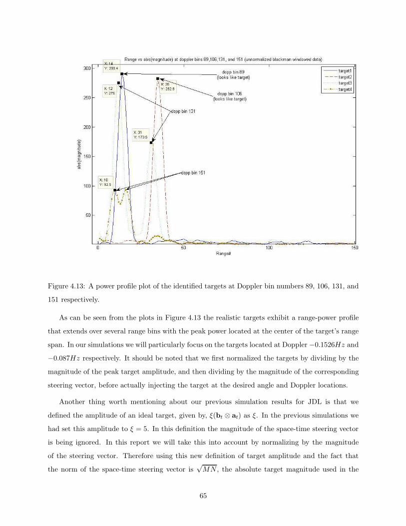
Figure 4.13: A power profile plot of the identified targets at Doppler bin numbers 89, 106, 131, and
151 respectively.
As can be seen from the plots in Figure 4.13 the realistic targets exhibit a range-power profile
that extends over several range bins with the peak power located at the center of the target’s range
span. In our simulations we will particularly focus on the targets located at Doppler −0.1526Hz and
−0.087Hz respectively. It should be noted that we first normalized the targets by dividing by the
magnitude of the peak target amplitude, and then dividing by the magnitude of the corresponding
steering vector, before actually injecting the target at the desired angle and Doppler locations.
Another thing worth mentioning about our previous simulation results for JDL is that we
defined the amplitude of an ideal target, given by, ξ(bt ⊗ at) as ξ. In the previous simulations we
had set this amplitude to ξ = 5. In this definition the magnitude of the space-time steering vector
is being ignored. In this report we will take this into account by normalizing by the magnitude
of the steering vector. Therefore using this new definition of target amplitude and the fact that
the norm of the space-time steering vector is√
MN , the absolute target magnitude used in the
65

Table 4.2: Target Characteristics
Target Parameters Ideal Target Real Target
Range(s) number 215 212-218
Amplitude(dB) 35 57
Azimuth(degrees) 35 35
Doppler(Hz) 0.18 0.18
previous JDL simulations is 20 log(ξ√
MN)
= 20 log(5√
4096 × 16)
= 62.14dB. Note that this
magnitude is an absolute magnitude and not a SNR.
Results
We begin this section by presenting some updated results of using JDL to identify both ideal and re-
alistic targets injected into the region dominated by Ionospheric clutter. It should be mentioned that
we conducted all our simulation results using the data-cube located in hfswrdata25mar2002030257.
The characteristics of the injected ideal and real targets are summarized in Table 4.2 To assess the
performance of the algorithms under scrutiny we will focus on the peak MSMI at the target range
and the difference in MSMI (in dB) between the peak MSMI and the second highest MSMI, de-
noted as ∆MSMI. The larger the ∆MSMI the larger the capability of an adaptive algorithm to
distinguish between a target and residual interference and thus the better is its performance. We
begin by presenting some of the updated JDL simulation results.
Figures 4.14 and 4.15 show the MSMI statistic vs range plots for the injected ideal target using
JDL. In Fig. 4.14 target amplitude is set to 35dB while in Fig. 4.15 the amplitude is set to 45dB.
These large values are the absolute numbers used and are not the target SNR. Note that, in both
figures, non-adaptive matched filtering cannot locate the injected target.
Figure 4.15 shows an MSMI vs range plot for the injected real target using JDL. It should be
mentioned that the results presented in these figures for JDL are for an optimal angle and Doppler
spacing obtained via a brute force search using a LPR composed of 3 angle and 10 Doppler bins.
Note that we also superposed on both figures plots of simulation results obtained via non-adaptive
matched filtering and adaptive Doppler processing. The adaptive Doppler processing algorithm
performs only spatial adaption (i.e., one dimensional adaption) after Doppler filtering while the
66

170 180 190 200 210 220 230 240 250 260 270
−20
−15
−10
−5
0
5
10
Range
MS
MI s
tatis
tic (
dB)
MSMI vs Range for a 35dB ideal target injected in Ionospheric Clutter Region
JDLAdaptive doppler−only processingNonadaptive MF
target
Figure 4.14: Results of using the JDL, Adaptive Doppler filter, and Nonadaptive MF algorithms
to detect an ideal target with amplitude 35dB inserted into the Ionospheric clutter region.
190 200 210 220 230 240 250 260 270
−20
−15
−10
−5
0
5
10
15
20
25
X: 215Y: 10.98
Range
MS
MI s
tatis
tic (
dB)
MSMI vs Range for a 45dB ideal target injected in the Ionospheric clutter region.
X: 215Y: 26.39
X: 215Y: 0.2786
JDLAdaptive doppler only processingNonadaptive MF
target
Figure 4.15: Results of using the JDL, Adaptive Doppler filter, and Nonadaptive MF algorithms
to detect an ideal target with amplitude 45dB inserted into the Ionospheric clutter region.
67

190 200 210 220 230 240 250 260
−20
−15
−10
−5
0
5
10
15
X: 215Y: 17.78
Range
MS
MI s
tatis
tic (
dB)
MSMI vs Range for real target injected in ionospheric clutter region
X: 215Y: 9.357
X: 215Y: −1.109
JDLAdaptive doppler filteringNonadaptive MF
57dBreal
target
Figure 4.16: Results of using the JDL, Adaptive Doppler filter, and Nonadaptive MF algorithms to
detect a real target spread over 7 range cells and with amplitude 57dB inserted into the Ionospheric
clutter region.
nonadaptive processing only does non-adaptive Doppler filtering. From the ideal target plot it
can be seen that JDL is capable of detecting the relatively weak target correctly even though the
target is buried deeply in a region of the angle-Doppler space that is heavily dominated by both
the ionospheric clutter as well as the high power external interference. The MSMI at the target is
almost 8dB above the surrounding clutter which emphasizes JDL’s ability to distinguish between
an ideal target and surrounding clutter. Both the non-adaptive matched filtering and adaptive
Doppler filtering methods fail at detecting the target. Our simulation results also indicated that
for higher target amplitudes JDL’s performance for the ideal target case by far exceeded that of
both the nonadaptive as well as the adaptive Doppler methods.
For the real target scenario (Figure 4.16) JDL also boasts better performance than that of
the adaptive Doppler filter and nonadaptive matched filters, however suffers a significant loss in
performance as compared to the case of an ideal target localized to only one range bin. The spread
of the target in range is accounted for by using a sufficient number of guard ranges (3 on either side
of each look range) thus minimizing the contribution of ranges containing target components to
the estimation of the interference covariance matrix. The peak MSMI of JDL in this case is 17.8dB
68

and the corresponding ∆ MSMI is about 4dB. Both the nonadaptive MF and adaptive Doppler
processor fail to detect the real target.
These new results echo the conclusions reached previously with the additional newly gained
confidence that JDL also has the capability to detect relatively weak realistic targets as well. Next
we present some of the simulation results obtained by applying the D3 and hybrid algorithms to
detect ideal and real targets injected at various locations in the data-cube under investigation.
In our simulations for the D3 and the hybrid and due to the large associated computational
load of these algorithms we decided to use an under-sampled in pulse version of the datacube. We
therefore used only 2048 of the 4096 pulses to run our simulations on the D3 algorithm and 1024
pulses for the hybrid algorithm. We conducted simulations for both ideal and real targets injected
into the region heavily dominated by ionospheric clutter. Figures 4.17 and 4.18 show the results of
applying D3 to the undersampled (in pulse) data-cube to detect ideal and realistic targets of peak
amplitude 55dB. D3 is incapable of detecting either the real or the ideal injected targets and shows
a rather poor performance relative to that of the Spatial adaptive processing algorithm. It should be
noted that using a higher power target will inevitably lead to a better detection performance by the
D3 algorithm however its performance will still lag behind that of any statistical based algorithm.
D3’s poor performance was anticipated since when used on its own, D3 is incapable of suppressing
the correlated interference present in each look range and thus will suffer a large degradation of
performance as compared to a statistical adaptive algorithm such as JDL, for example.
We next went on to evaluate the performance of the hybrid algorithm in detecting ideal and real
targets inserted into the region dominated by high power ionospheric clutter returns. Figures 4.19
and 4.20 show the results of using the Hybrid algorithm to detect an ideal and real target injected
in the ionospheric region. As can be verified from the results the hybrid algorithm is capable of
detecting both the ideal and real targets quite nicely. In fact it outperforms JDL in both the real
and ideal cases. For the ideal target the hybrid algorithm yields a very good detection criterion, at
the target range, of 32.45dB which is about 2.5dB greater than that of JDL. It also yields a superior
∆ MSMI. In the real target scenario JDL fails to detect the target while the hybrid algorithm does
so with about a 1dB margin. Note that we are using one fourth of the available number of pulses,
and we are still getting quite good results for the hybrid algorithm. Thus the hybrid does a good
job of suppressing any uncorrelated interference present in the look range after which it uses the
second stage of the statistical JDL algorithm to null out any correlated interference that might be
69
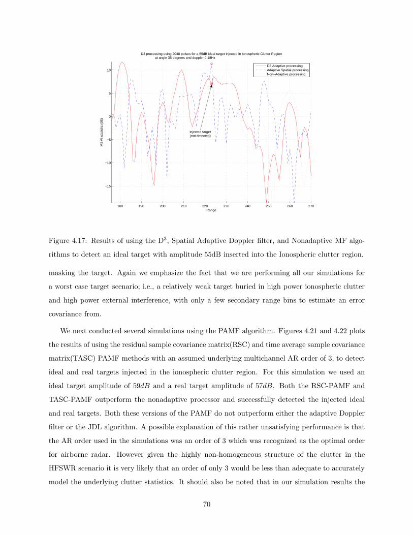
180 190 200 210 220 230 240 250 260 270
−15
−10
−5
0
5
10
Range
MS
MI s
tatis
tic (
dB)
D3 processing using 2048 pulses for a 55dB ideal target injected in Ionospheric Clutter Regionat angle 35 degrees and doppler 0.18Hz
D3 Adaptive processingAdaptive Spatial processingNon−Adaptive processing
injected target(not detected)
Figure 4.17: Results of using the D3, Spatial Adaptive Doppler filter, and Nonadaptive MF algo-
rithms to detect an ideal target with amplitude 55dB inserted into the Ionospheric clutter region.
masking the target. Again we emphasize the fact that we are performing all our simulations for
a worst case target scenario; i.e., a relatively weak target buried in high power ionospheric clutter
and high power external interference, with only a few secondary range bins to estimate an error
covariance from.
We next conducted several simulations using the PAMF algorithm. Figures 4.21 and 4.22 plots
the results of using the residual sample covariance matrix(RSC) and time average sample covariance
matrix(TASC) PAMF methods with an assumed underlying multichannel AR order of 3, to detect
ideal and real targets injected in the ionospheric clutter region. For this simulation we used an
ideal target amplitude of 59dB and a real target amplitude of 57dB. Both the RSC-PAMF and
TASC-PAMF outperform the nonadaptive processor and successfully detected the injected ideal
and real targets. Both these versions of the PAMF do not outperform either the adaptive Doppler
filter or the JDL algorithm. A possible explanation of this rather unsatisfying performance is that
the AR order used in the simulations was an order of 3 which was recognized as the optimal order
for airborne radar. However given the highly non-homogeneous structure of the clutter in the
HFSWR scenario it is very likely that an order of only 3 would be less than adequate to accurately
model the underlying clutter statistics. It should also be noted that in our simulation results the
70
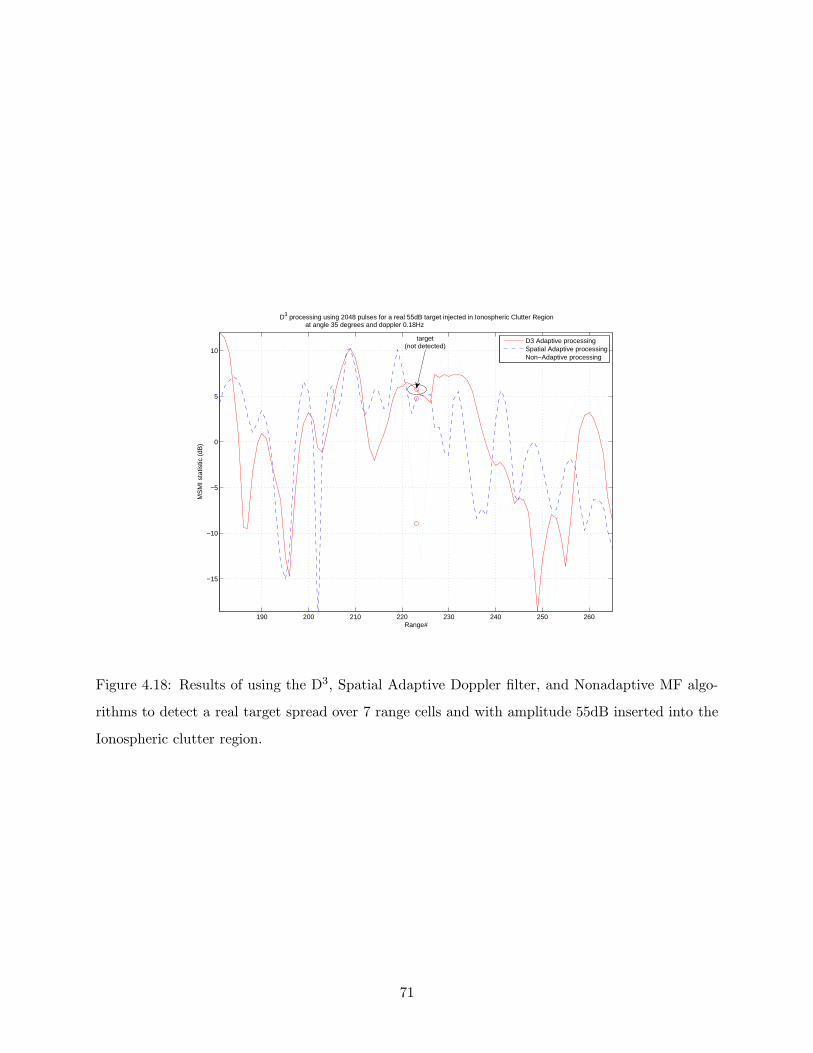
190 200 210 220 230 240 250 260
−15
−10
−5
0
5
10
Range#
MS
MI s
tatis
tic (
dB)
D3 processing using 2048 pulses for a real 55dB target injected in Ionospheric Clutter Region at angle 35 degrees and doppler 0.18Hz
D3 Adaptive processingSpatial Adaptive processingNon−Adaptive processing
target(not detected)
Figure 4.18: Results of using the D3, Spatial Adaptive Doppler filter, and Nonadaptive MF algo-
rithms to detect a real target spread over 7 range cells and with amplitude 55dB inserted into the
Ionospheric clutter region.
71

180 190 200 210 220 230 240 250 260 270
−30
−20
−10
0
10
20
30
Range
MS
MI s
tatis
tic (
dB)
Hybrid processing using 1024 pulses for an ideal 55dB target injected in Ionospheric Clutter Region, with 3 angle bins and 10 Doppler bins, and K = 94 samples.and optimal interdoppler spacing= 0.00012256 ,optimal interangle spacing =0.25923
D3
HybridJDLAdapive SpatialNonadaptive
Figure 4.19: Results of using the Hybrid,D3,JDL, Spatial Adaptive Doppler filter, and Nonadaptive
MF algorithms to detect an ideal target with amplitude 55dB inserted into the Ionospheric clutter
region.
RSC-PAMF does a better job at detecting the injected target than the TASC-PAMF method.
4.5.1 Discussion on STAP Algorithms
In the area of applying STAP to ionospheric clutter, in this report we presented new simulation
results of using several STAP algorithms to suppress high power nonhomogeneous clutter returns
from the highly non-stationary ionospheric layers. We began by incorporating real targets into our
simulations and testing the various algorithms to see how well they fare against realistic targets.
In particular we ran several tests on the JDL algorithm to evaluate its realistic target detection
capabilities. Our simulation results indicate that JDL does a good job at detecting such targets
even when they are spread over up to 7 range bins.
We also implemented and tested 3 new algorithms in this report, namely the D3 algorithm, the
Hybrid algorithm, and the PAMF algorithm. The D3 did not perform well for both ideal and real
targets. This was expected given the algorithm’s weakness against correlated clutter that seems
to be the dominant type of clutter in the ranges we analyzed. The Hybrid algorithm on the other
hand showed very good detection performance for both ideal, and more importantly, real targets.
72

190 200 210 220 230 240 250 260
−25
−20
−15
−10
−5
0
5
10
Range
MS
MI s
tatis
tic (
dB)
Hybrid processing using 1024 pulses, for a real 55dB target injected in the Ionospheric Clutter Region: with 3 angle bins and 10 Doppler bins, and K = 88 samples. optimal interdoppler spacing= 0.00012256 ,optimal interangle spacing =0.25923
D3
HybridJDLSpatial AdaptiveNonadaptive
real target (detected)
Figure 4.20: Results of using the Hybrid,D3,JDL, Spatial Adaptive Doppler filter, and Nonadaptive
MF algorithms to detect a real target spread over 7 range cells and with amplitude 55dB inserted
into the Ionospheric clutter region.
The Hybrid outperformed JDL and all the other tested methods and so far seems to yield the best
performance among the algorithms we tested. It is well known that the Hybrid algorithm yield
superior results in airborne radar, but our investigations seem to strongly affirm that the Hybrid
is also a robust and well performing algorithm in HFSWR applications.
The final algorithm we investigated was the PAMF algorithm which highly depends on as-
sumptions made about the nature of the underlying clutter. Assuming the clutter to be an AR(p)
process (which may not be completely justified in the case of ionospheric highly non-homogeneous
clutter), we had to select an appropriate order p that yields a sufficiently accurate representation
of the clutter statistics. We used an AR order of 3 in our simulations,which is the optimal order
for airborne radar. The results obtained with this choice of order and using the PAMF algorithm
for ideal and real target detection in the ionospheric region, yielded some modest results that were
by no mean striking to us.
The next section describes a key contribution of this report - the development of the Fast Fully
Adaptive algorithm, an extremely efficient scheme based on the Fast Fourier Transform (FFT)
73

190 200 210 220 230 240 250 260 270−20
−15
−10
−5
0
5
10
15
20
MS
MI s
tatis
tic (
dB)
Range#
MSMI vs Range for a 59dB ideal target injected in the Ionospheric clutter dominated region.
PAMF Adaptive processing (Least Squares Residual Covariance method)PAMF Adaptive processing (Least Squares Time Average Sample method)NonadaptiveAdaptive doppler processing
Figure 4.21: Results of using the RSC-PAMF, TASC-PAMF, Adaptive Doppler filter, and Non-
adaptive MF algorithms to detect an ideal point target with amplitude 59dB inserted into the
Ionospheric clutter region.
4.6 Fast Fully Adaptive Algorithm
In the previous section we provided results of Monte Carlo simulation to evaluate the processing
gain of the non-adaptive, spatially adaptive, JDL and parametric adaptive matched filter (PAMF)
methods to detect weak targets embedded within the ionospheric clutter that dominates the far
ranges of the measured data sets. We also addressed the problem related to the aliasing in pulse
due to downsampling without low pass filtering. We then provided a brief complexity analysis of
the JDL and Hybrid algorithms. We provided several simulation results that validated our previous
work.
In this section we introduce the new FFA algorithm and perform a complexity analysis which
we contrast against that of the JDL algorithm. We also evaluate the performance of the FFA
algorithm and compare it to that of non-adaptive and JDL methods for HFSWR. We begin by
developing the FFA algorithm for a general linear array of isotropic point sensors processing M
coherent pulses as in the original STAP work of Ward [44].
74

190 200 210 220 230 240 250 260
−25
−20
−15
−10
−5
0
5
10
15
MS
MI s
tatis
tic (
dB)
Range#
MSMI vs Range for a 63dB real target injected in the Ionospheric clutter dominated region.
PAMF Adaptive processing (Least Squares Residual Covariance method)PAMF Adaptive processing (Least Squares Time Average Sample method)NonadaptiveAdaptive doppler processing
target
Figure 4.22: Results of using the RSC-PAMF, TASC-PAMF, Adaptive Doppler filter, and Non-
adaptive MF algorithms to detect a real target spread over 7 range cells and with amplitude 63dB
inserted into the Ionospheric clutter region.
4.6.1 System Model
Since the primary focus of this project is the adaptive suppression of ionospheric clutter in HFSWR
applications, we will only evaluate our method using the measured HFSWR data made available
to us through Dr. Riddolls. We will treat the combined effects of all clutter sources as colored
noise. Ideal targets in the HFSWR scenario can be modeled (quite accurately) in a fashion similar
to targets in airborne applications (i.e., point sources localized in azimuth, doppler, and range),
and as a result we will use the conventional space-time steering vector, developed in the airborne
radar literature [44], to model target returns in HFSWR.
To develop the FFA algorithm, we will adopt the conventional STAP setup. The receiver
comprises N spatial channels separated by a distance of λ/2, processing over M coherent pulses
with a pulse repetition frequency (PRF) of fp. The data comprises any potential target, background
clutter (including sea and ionospheric clutter), interference, and receiver noise. This process is
repeated for the numerous ranges of interest, and the corresponding N × M space-time snapshots
at each range are compiled into one big data-cube. For a specific range bin, r, the N × M data
75

matrix is given by:
X = ξV + C + N,
V = a(ϕt) ⊗ bT (ft),
a(ϕt) = [ 1 zs · · · z(N−1)s ]
T
b(ft) = [ 1 zt · · · z(M−1)t ]
T
zs = ei2π(d/λ) sin(ϕt),
zt = ei2π(ft/fR),
(4.63)
where ξ is the target amplitude, a(ϕt) and b(ft) are the target spatial and temporal steering vectors
respectively, at azimuth ϕt and doppler ft , and C and N represent the clutter and noise space-time
contributions respectively. The value of ξ is either zero under the null hypothesis (i.e., no target
present) or nonzero for the case when a target is present.
Ideally a target (if present) is localized in range to one range bin, however in real systems the
radar ambiguity function leads to a spread of the target over several ranges, and this spread must
be accounted for in the target model. It should be noted that for the HFSWR system considered
here, the radar waveform consists of a complementary set of 8 phase code pulses. Each of the 8
pulses in turn consists of 8 bits, where each bit is 55 microseconds long, and thus each pulse is
440 microseconds long. Thus in order to account for the spread of the target in range we also
use a realistic target space-time vector which is spread over range and extracted from actual real
high-SNR target returns present in separately measured data cubes. The target signal is extracted
using a matched filter, localizing the target in Doppler.
4.6.2 Fast Fully Adaptive Algorithm
We will begin by briefly describing the optimal MF method and AMF method, since they constitute
the core of the FFA method. Assuming prior knowledge of the interference statistics, and as a
result of the error covariance matrix R, the matched filter solution leads to the computation of the
following optimal weight vector,
wopt = R−1v, (4.64)
where R is the known interference covariance matrix and v is the space-time steering vector at the
angle and Doppler of interest. The vector v is the vectorized version of space-time steering matrix
V used in Eqn. 4.63.
76
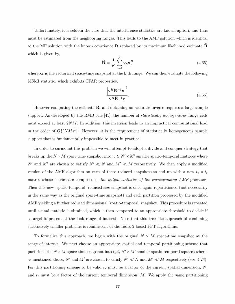
Unfortunately, it is seldom the case that the interference statistics are known apriori, and thus
must be estimated from the neighboring ranges. This leads to the AMF solution which is identical
to the MF solution with the known covariance R replaced by its maximum likelihood estimate R
which is given by,
R =1
K
K∑
r=1
xkxHk (4.65)
where xk is the vectorized space-time snapshot at the k’th range. We can then evaluate the following
MSMI statistic, which exhibits CFAR properties,∣∣∣vHR−1x
∣∣∣2
vHR−1v. (4.66)
However computing the estimate R, and obtaining an accurate inverse requires a large sample
support. As developed by the RMB rule [45], the number of statistically homogeneous range cells
must exceed at least 2NM . In addition, this inversion leads to an impractical computational load
in the order of O{(NM)3}. However, it is the requirement of statistically homogeneous sample
support that is fundamentally impossible to meet in practice.
In order to surmount this problem we will attempt to adopt a divide and conquer strategy that
breaks up the N×M space time snapshot into ts.tt N ′×M ′ smaller spatio-temporal matrices where
N ′ and M ′ are chosen to satisfy N ′ ≪ N and M ′ ≪ M respectively. We then apply a modified
version of the AMF algorithm on each of these reduced snapshots to end up with a new ts × tt
matrix whose entries are composed of the output statistics of the corresponding AMF processes.
Then this new ’spatio-temporal’ reduced size snapshot is once again repartitioned (not necessarily
in the same way as the original space-time snapshot) and each partition processed by the modified
AMF yielding a further reduced dimensional ’spatio-temporal’ snapshot. This procedure is repeated
until a final statistic is obtained, which is then compared to an appropriate threshold to decide if
a target is present at the look range of interest. Note that this tree like approach of combining
successively smaller problems is reminiscent of the radix-2 based FFT algorithms.
To formalize this approach, we begin with the original N × M space-time snapshot at the
range of interest. We next choose an appropriate spatial and temporal partitioning scheme that
partitions the N×M space-time snapshot into ts.tt N ′×M ′ smaller spatio-temporal squares where,
as mentioned above, N ′ and M ′ are chosen to satisfy N ′ ≪ N and M ′ ≪ M respectively (see 4.23).
For this partitioning scheme to be valid ts must be a factor of the current spatial dimension, N ,
and tt must be a factor of the current temporal dimension, M . We apply the same partitioning
77
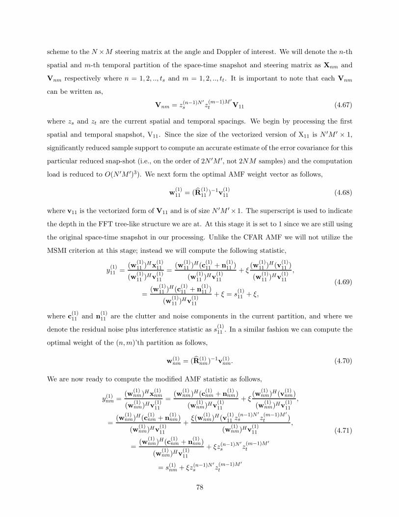
scheme to the N ×M steering matrix at the angle and Doppler of interest. We will denote the n-th
spatial and m-th temporal partition of the space-time snapshot and steering matrix as Xnm and
Vnm respectively where n = 1, 2, .., ts and m = 1, 2, .., tt. It is important to note that each Vnm
can be written as,
Vnm = z(n−1)N ′
s z(m−1)M ′
t V11 (4.67)
where zs and zt are the current spatial and temporal spacings. We begin by processing the first
spatial and temporal snapshot, V11. Since the size of the vectorized version of X11 is N ′M ′ × 1,
significantly reduced sample support to compute an accurate estimate of the error covariance for this
particular reduced snap-shot (i.e., on the order of 2N ′M ′, not 2NM samples) and the computation
load is reduced to O(N ′M ′)3). We next form the optimal AMF weight vector as follows,
w(1)11 = (R
(1)11 )−1v
(1)11 (4.68)
where v11 is the vectorized form of V11 and is of size N ′M ′×1. The superscript is used to indicate
the depth in the FFT tree-like structure we are at. At this stage it is set to 1 since we are still using
the original space-time snapshot in our processing. Unlike the CFAR AMF we will not utilize the
MSMI criterion at this stage; instead we will compute the following statistic,
y(1)11 =
(w(1)11 )Hx
(1)11
(w(1)11 )Hv
(1)11
=(w
(1)11 )H(c
(1)11 + n
(1)11 )
(w(1)11 )Hv
(1)11
+ ξ(w
(1)11 )H(v
(1)11 )
(w(1)11 )Hv
(1)11
,
=(w
(1)11 )H(c
(1)11 + n
(1)11 )
(w(1)11 )Hv
(1)11
+ ξ = s(1)11 + ξ,
(4.69)
where c(1)11 and n
(1)11 are the clutter and noise components in the current partition, and where we
denote the residual noise plus interference statistic as s(1)11 . In a similar fashion we can compute the
optimal weight of the (n,m)’th partition as follows,
w(1)nm = (R(1)
nm)−1v(1)nm. (4.70)
We are now ready to compute the modified AMF statistic as follows,
y(1)nm =
(w(1)nm)Hx
(1)nm
(w(1)nm)Hv
(1)11
=(w
(1)nm)H(c
(1)nm + n
(1)nm)
(w(1)nm)Hv
(1)11
+ ξ(w
(1)nm)H(v
(1)nm)
(w(1)nm)Hv
(1)11
,
=(w
(1)nm)H(c
(1)nm + n
(1)nm)
(w(1)nm)Hv
(1)11
+ξ(w
(1)nm)H(v
(1)11 z
(n−1)N ′
s z(m−1)M ′
t )
(w(1)nm)Hv
(1)11
,
=(w
(1)nm)H(c
(1)nm + n
(1)nm)
(w(1)nm)Hv
(1)11
+ ξz(n−1)N ′
s z(m−1)M ′
t
= s(1)nm + ξz(n−1)N ′
s z(m−1)M ′
t
(4.71)
78

where we made use of the relation in 4.67 between the (n,m)-th steering matrix partition and the
first steering matrix partition. Defining z{1}s and z
{1}t as follows,
z{1}s = zN ′
s
z{1}t = zM ′
t
(4.72)
and comparing y(1)11 and y
(1)nm, we notice that the residual signal component of y
(1)nm is (z
{1}s )n−1(z
{1}t )m−1
times the residual signal component of y(1)11 . This indicates that through our careful choice of a
modified statistic, we have preserved the phase relationship between the residual signal components
of different spatio-temporal partitions after being processed through the modified AMF filters. We
can thus regard the resulting ts × tt matrix as a new ’spatio-temporal’ snapshot with a fraction
of the temporal and spatial degrees of freedom (DoF) of the original space-time snapshot, and
containing a target with the same amplitude but with new Doppler and angle phase shifts given by
z{1}t and z
{1}s respectively.
Choosing a new set of spatial and temporal partitions for the resulting spatio-temporal matrix
at each depth, and repeating the modified AMF algorithm on each of these partitions, will sys-
tematically lead to the evaluation of a final detection statistic which indirectly incorporates all the
DoF of the original data-cube at different depths of the algorithm. However the resulting statistic
is not CFAR. To overcome this problem we use the MSMI CFAR statistic as the detection statistic
computed at the final stage of the algorithm where only one final spatio-temporal partition remains.
This has the effect of making the final statistic CFAR. It should also be mentioned that at every
depth we must also ’modify’ the secondary data appropriately. To accomplish this we perform
the same computation, conducted at the look range of every partition, to all the corresponding
spatio-temporal partitions at all the secondary ranges used.
4.6.3 Complexity Analysis
The FFA algorithm yields significant improvement in computation speed load compared to the
practically un-achievable AMF. However the real test of valor will be a comparison of the complexity
of the FFA Algorithm to other STAP algorithms that have been designed for their low computation
load, such as the JDL algorithm. It is somewhat difficult to compare complexities of algorithms that
have numerous defining parameters such as the number of angle and doppler bins that dictate the
complexity of JDL, or the spatio-temporal partition sequence choice that almost fully characterizes
the complexity and performance of the FFA Algorithm. Nonetheless, we will attempt to provide
79
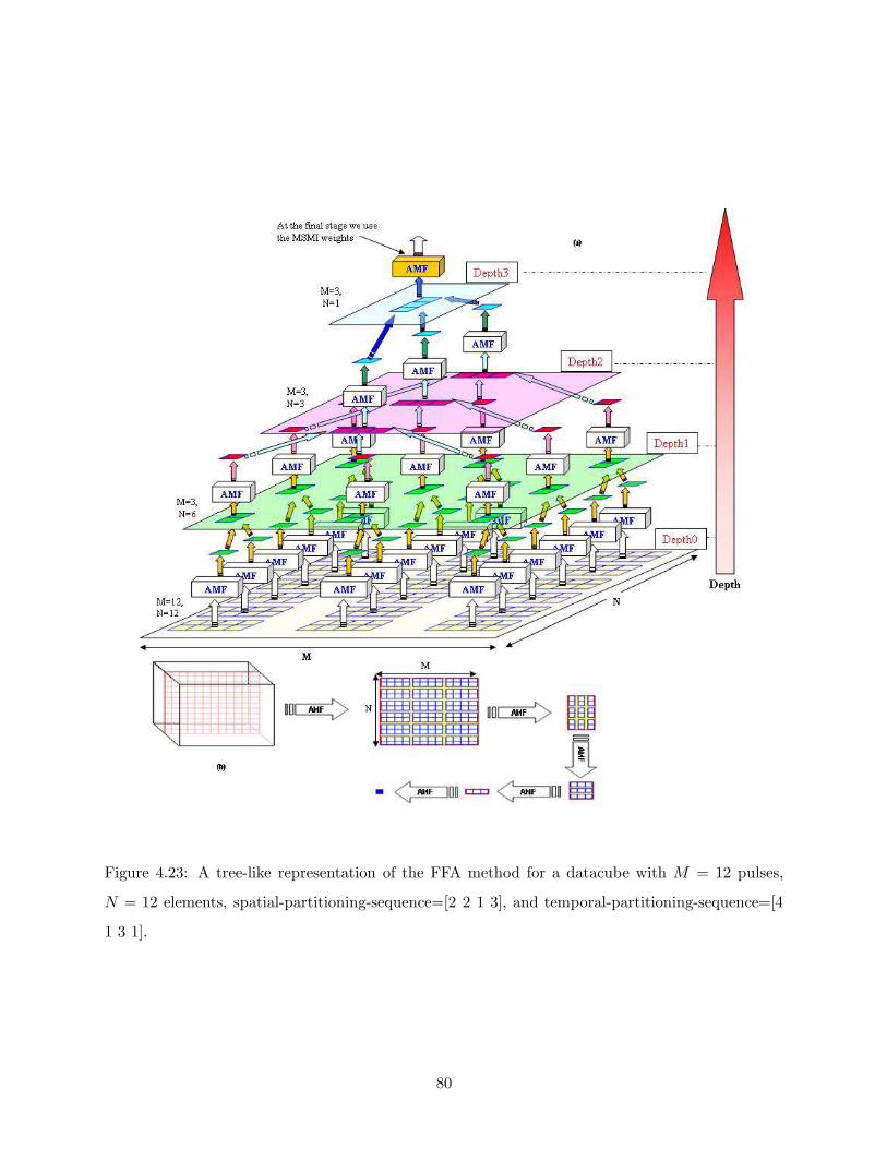
Figure 4.23: A tree-like representation of the FFA method for a datacube with M = 12 pulses,
N = 12 elements, spatial-partitioning-sequence=[2 2 1 3], and temporal-partitioning-sequence=[4
1 3 1].
80

some sense of complexity evaluation that, in turn, will better allow us to characterize the utility
of our algorithm in practical STAP scenarios. The algorithm we choose to compare complexity
against is the JDL algorithm since it is a reduced dimension algorithm that has been designed
with a particular focus on reduction of complexity. As a starting point we will derive the ’generic’
expression defining the complexity of JDL and the FFA Algorithm in terms of their corresponding
parameters.
Beginning with JDL, we assume a local processing region (LPR) comprising ηa angle bins and
ηd Doppler bins. Reducing the size of the LPR leads to a reduction in the computation times of
the JDL algorithm, but also leads to a loss of performance. The algorithm running time for one
look range can be approximated as TJDL = ηaηd(T1) + ǫ where T1 is the time needed to compute 1
column entry of the JDL transformation matrix, and ǫ is the time needed to perform inversion of
the covariance matrix and is a function of O((ηaηd)3). However the transformation matrix needs to
be computed only once, and not for every look range. Consequently for r look ranges the running
time of JDL would approximately be ηaηd(T1) + rO((ηaηd)3).
Next we derive the complexity of the FFA Algorithm. In essence its complexity for a spatio-
temporal partition of size N ′ × M ′ is that of the AMF and is primarily defined by the complexity
associated with the inversion of an N ′M ′ × N ′M ′ matrix, and is therefore O((N ′M ′)3). This
process is repeated tds.tdt times at every depth, d, where tds must be a factor of N and tdt must be
a factor of M . Thus assuming a given spatial partitioning sequence SN = {n1, n2, ..., nmax(kN ,kM )}and a temporal partitioning sequence SM = {m1,m2, ...,mmax(kN ,kM)}, where mi and ni are the
spatial and temporal dimensions of the partitions at depth i, and kN and kM are the largest non-
unit spatial and temporal factor indices respectively. In order to make both spatial and temporal
sequences of the same size we augment the shorter sequence with 1′s until both sequences are the
same length. Thus the maximum depth of the FFT-like tree is given by max(kN , kM ). As a result
the complexity of the FFA per range can be written as,
TFFA =
max(kN ,kM )∑
d=1
NMd∏
i=1nimi
O((ndmd)
3)
=
max(kN ,kM )∑
d=1
{(max(kN ,kM )∏
i=d
nimi
)O((ndmd)
2)}
(4.73)
and since this process must be repeated for all look ranges, then for r ranges the running time
would be rTFFA. As can be seen by comparing the 2 expressions outlining the complexities of
the 2 algorithms being evaluated, it is not straight forward to draw a definite conclusion. We
81

Table 4.3: Average Running Time of various algorithms per look range per look angle per look
doppler
Algorithm Avg Running Time(sec)
Nonadaptive 0.005
Spatial Adaptive 0.007
JDL (with 3 angle and 11 doppler bins) 0.57
D3 (using 2048 pulses) 15.35
PAMF(with AR order of 5) 6.66
Hybrid(using 2048 pulses with 3 angle and 11 doppler bins) 497.25
FFA 2.8404
can manipulate the various parameters of each algorithm to favor either algorithm, in terms of
complexity. However the performance is directly related to the parameters and is often characterized
by an inverse relationship with the complexity, and therefore a tradeoff is inevitable. In general, in
terms of computation load, JDL has the distinct advantage that it requires the solution of single
size-ηaηd matrix while the FFA approach requires several AMF solutions. On the other hand, in
terms of performance, the FFA algorithm uses all NM adaptive DoF while the JDL is restricted
to just ηaηd.
Table 4.3 shows some example average running times for the FFA, JDL, Hybrid, D3, and
PAMF methods obtained from simulations using the measured data-cubes made available to us by
the DRDC. The processor used is a DuoCore2 processor with 2GB of RAM and a speed of 2.13GHz
running the Windows XP operating system.
The above JDL results are for 11 doppler bins and 3 angle bins, and the FFA results are for a
spatial-partitioning-sequence= [2, 2, 2, 2] and a temporal-partitioning-sequence= [4, 4, 16, 16]. Note
that the time results for D3 and hybrid algorithms are for a decimated datacube by a factor of
4, and the result for the PAMF algorithm is for an assumed AR order of 5. Also we are using a
LPR composed of ηa = 3 angle bins and ηd = 11 doppler bins. In this case JDL is about 78%
faster than FFA for the chosen partitioning scheme. It should be noted that the FFA program used
in our simulations has not yet been optimized for minimal running time, while the JDL program
has undergone code optimization. However comparing the FFA (for this particular partitioning
82

scheme)to the Hybrid, D3, and PAMF methods we can see a significant speedup. Furthermore, as
we will see, the performance of FFA algorithm is hugely superior to that of the JDL algorithm.
It should be noted that for the FFA method to yield complexity reductions both N and M
must have factors that are relatively small (for example both N and M are powers of 2 - this is
similar to that required by the FFT algorithm).
4.6.4 Simulation Results
In this section we will evaluate the performance of the FFA algorithm in the HFSWR setup using
both ideal point targets and realistic targets spread in range. We will provide MSMI statistic versus
Range plots to characterize the performance of our algorithm and compare it to that of the non-
adaptive and JDL methods. We will thus inject ideal and real targets at specific locations in the
datacube, and use the three methods to attempt to detect the injected target. We will also focus
on the difference between the target MSMI statistic (assumed to be the largest) and the second
largest MSMI statistic, termed ∆ MSMI, which we will use as a sensitivity measure i.e., the larger
the ∆ MSMI of a certain algorithm, the larger its ability to distinguish a target from a background
of interference and noise. Since we neither have sufficient measured data to evaluate a detection
threshold for a given probability of false alarm, nor the capability to generate such data due to the
absence of an accurate model for ionospheric clutter, we will only declare a target detection to be
successful if the MSMI statistic at the target range is the maximum among the look ranges being
scanned for targets. We will begin with the ideal target scenario, where we inject a weak ideal
point target into the measured HFSWR data cubes, to test the target detection capability of each
of the FFA,Nonadaptive, and JDL methods.
In our example, we inject our ideal 45dB target at range number 223 which is at the center of the
ionospheric clutter region, at an angle of 35◦ which is within the external interference angle span,
and at a Doppler of 0.18Hz which coincides with the Bragg-Line Doppler frequency of the data-cube
at hand. It is important to note that 45dB measures the absolute amplitude of the injected target,
as opposed to the SINR. It should also be noted that due to the large number of pulses (4096) it is
computationally impossible to produce MSMI versus range plots for the AMF since the inversion of
the associated covariance would be on the order of O((MN)3) = O(2.8147e+014). Instead we focus
on a comparison between the performance of the FFA method and that of JDL and nonadaptive
processing. Figure 4.25 shows the detection results for the methods being investigated. For this
83

simulation the spatial-partitioning sequence and temporal-partitioning sequence we selected for
FFA are [2, 2, 2, 2] and [4, 4, 16, 16] respectively, and the JDL parameters are the same ones used
in the airborne radar simulations presented earlier. As can be seen from Fig. 4.25 the nonadaptive
algorithm fails at detecting the target, while both the FFA and JDL methods do successfully detect
the presence of a target. However it is evident from examining the curves that the FFA shows about
a 10dB improvement in ∆ MSMI as compared to JDL, which emphasizes the FFA’s superior target
discrimination capabilities. It should be noted that the FFA results for this simulation are for
only one possible spatio-temporal partition sequence, which has not been optimized in any way.
We therefore expect that there exists other spatio-temporal sequences that may yield even larger
improvements in performance and push the performance boundary even closer to that of the AMF
with ample sample support. We next investigate how the FFA fairs in a reduced DoF scenario
where we use only a fraction of the available 4096 pulses for target detection. Figure 4.26 plots
the MSMI versus range curves for the FFA, JDL, and Nonadaptive methods using only 128 out
of the 4096 available pulses (i.e., a reduction by a factor of 32). Once again the non-adaptive
method fails, while both the FFA and JDL methods succeed at localizing the target. Note that
due to the decimation in pulse, the performance of both algorithms is worse than before, however
the FFA still outperforms the JDL by a ∆ MSMI margin of about 3.5dB, again asserting its
superior target discrimination capacity. It should be mentioned that for this simulation we used a
spatial-partitioning sequence of [2, 2, 2, 2] and temporal-partitioning sequence of [2, 4, 4, 4] for the
FFA method.
We next investigate the performance of the FFA method for real target scenarios. In this
simulation we inject real targets spread over several ranges, which have been extracted from actual
target returns present in the data-cubes made available to us by the DRDC. We use the same FFA
and JDL parameters used in the ideal target simulation utilizing all 4096 pulses. The results are
shown in Fig. 4.27, where it is evident that both the nonadaptive as well as the JDL methods fail
to detect the buried real target while the FFA method successfully does so with a ∆ MSMI margin
of 12.8dB. We next repeat the simulations for a reduced pulse scenario. Again we use the same
setup outlined in the decimated in pulse ideal target case. The results are shown in Fig. 4.28, and
once again indicate that only the FFA method can successfully detect the real target and does so
with a margin of more than 8dB.
To further illustrate the superiority of the FFA method, we produce ∆ MSMI vs Target Ampli-
84

25 30 35 40 45 50 55 600
5
10
15
20
25
30
35
40
X: 56Y: 21.2
∆MSMI vs Target Amplitude for the JDL and FFA methods from ideal targets injected in the Ionospheric region of the HFSWR datacube using 18 iterations per SNR.(N=16, M=4096, K=94, (η
a,η
d, ∆a, ∆f) =(3,11,1/(N*sqrt(2)),1/(M*sqrt(2))), temporal−spacing=[4 4 16 16] , spatial−spacing=[2 2 2 2] )
Target Amplitude(dB)
∆MS
MI(
dB)
X: 56Y: 32.48
JDLFFA
approximately 10dB
slope=0.996
slope=0.977
Non−Linear Region Linear Region
Figure 4.24: ∆MSMI versus target amplitude for JDL, and FFA algorithms
tude plots for both the JDL and FFA algorithm. We use 18 (a relatively small number) iterations
per target amplitude to obtain the curve. The range of Target Amplitudes we scan over is from
25dB to 60dB in steps of 1dB. Again since we have no means to determine the actual noise power,
we use Target Amplitude as a proxy for SNR. Figure 4.24 shows the results for the JDL and FFA
methods. In this simulation we use 3 angle and 11 doppler bins for the JDL method and a spatial
and temporal partitioning sequence of [2, 2, 2, 2] and [4, 4, 16, 16] respectively for the FFA method.
The JDL’s nonlinear region seems to extend well into the linear region of the FFA method before
itself entering into its linear region(at around 44dB target amplitude). The slope of both curves in
their linear region is very close to 1, and the difference between the curves is approximately 10dB
in the linear region. These results reemphasize the superior performance of the FFA method in a
more credible fashion.
These simulations indicate that the FFA method appears to be a highly practical method that
performs well in real target detection scenarios under limited sample support, few available DoF,
and at a relatively low complexity for HFSWR applications.
The FFA algorithm as reviewed here was shown to provide significant performance gains over
other reduced DoF schemes such as JDL [11]. The next section describes a generalization of this
scheme wherein the partitions are interleaved with each other.
85

180 190 200 210 220 230 240 250 260 270
−10
0
10
20
30
40
X: 223Y: 41.27
X: 223Y: 27.79
X: 176Y: 10.67
X: 200Y: 6.273
MSMI vs Range using 45dB ideal target(N=16,M=4096,K=94), FFA(spatial−partition−sequence=[2 2 2 2],temporal−partition−sequence=[4 4 16 16])JDL(η
a=3, η
d=11, doppler−sepp=1/Msqrt(2), angle−sepp=1/Nsqrt(2) )
JDLFFANonadaptive
Figure 4.25: MSMI vs Range plots for using the Nonadaptive, JDL, and FFA methods to detect
an ideal target in Ionospheric clutter region. All 4096 pulses are used in this simulation.
4.7 Interleaved FFA Description
In this section we will develop a more general partitioning scheme for the FFA method. We will
denote this new partitioning method when combined with the FFA method as the Interleaved FFA
method for reasons that will become obvious shortly. In the regular FFA method described above
we partitioned the spatial and temporal dimensions at each depth into disjoint partitions whose
union resulted in the original spatio-temporal data cube. However it is not imperative that the
partitions be disjoint, and it is possible to select a partitioning scheme in which the different spatial
and/or temporal partitions overlap, thus reusing the same DoF more than once in each of the
overlapping partitions.
To formalize this scheme, we begin with several definitions(refer to Figure 4.29). We define dN
and dM as the length of the spatial and temporal partitions respectively at a certain depth of the
FFA tree. Next we define sN and sM as the distance between two consecutive spatial and temporal
partitions. Figure 4.29 might represent either the data-matrix of space-time samples at a certain
depth or the corresponding steering matrix in the direction of the look angle and doppler.
In the example shown in Fig. 4.29, dN = 3, sN = 2, dM = 5, and sM = 3. If we assume the
space-time matrix in Fig. 4.29 to represent the steering matrix at a certain depth, where zs and zt
are the current spatial and temporal spacings, we can write the spatio-temporal partition steering
86
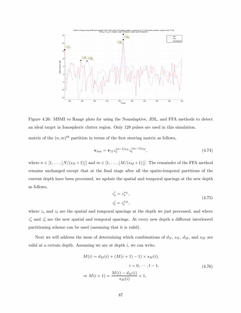
180 190 200 210 220 230 240 250 260 270
−15
−10
−5
0
5
10
15
20
25
X: 223Y: 22.26
Range
MS
MI s
tatis
tic (
dB)
MSMI vs Range using 45dB ideal target(N=16,M=128,K=94), FFA(spatial−partition−sequence=[2 2 2 2],temporal−partition−sequence=[2 4 4 4])JDL(η
a=3, η
d=11, doppler−sepp=1/Msqrt(2), angle−sepp=1/Nsqrt(2) )
X: 223Y: 25.65
X: 194Y: 8.489
X: 176Y: 15.77
X: 189Y: 8.771
JDLFFANonadaptive
Figure 4.26: MSMI vs Range plots for using the Nonadaptive, JDL, and FFA methods to detect
an ideal target in Ionospheric clutter region. Only 128 pulses are used in this simulation.
matrix of the (n,m)th partition in terms of the first steering matrix as follows,
vnm = v11z(n−1)sNs z
(m−1)sM
t , (4.74)
where n ∈ [1, . . . , ⌊N/(sN +1)⌋] and m ∈ [1, . . . , ⌊M/(sM +1)⌋]. The remainder of the FFA method
remains unchanged except that at the final stage after all the spatio-temporal partitions of the
current depth have been processed, we update the spatial and temporal spacings at the new depth
as follows,
z′s = zsNs ,
z′t = zsM
t ,(4.75)
where zs and zt are the spatial and temporal spacings at the depth we just processed, and where
z′s and z′t are the new spatial and temporal spacings. At every new depth a different interleaved
partitioning scheme can be used (assuming that it is valid).
Next we will address the issue of determining which combinations of dN , sN , dM , and sM are
valid at a certain depth. Assuming we are at depth i, we can write,
M(i) = dM (i) + (M(i + 1) − 1) × sM (i),
i = 0, · · · , t − 1,
⇒ M(i + 1) =M(i) − dM (i)
sM (i)+ 1,
(4.76)
87

190 200 210 220 230 240 250 260−25
−20
−15
−10
−5
0
5
10
15
20
X: 223Y: 24.01
Range
MS
MI s
tatis
tic (
dB)
MSMI vs range for a 45dB real target injected in Ionospheric clutter region for a decimated in pulse datacube of 4096 pulses.(N=16,M=4096, K=85,11 doppler bins, 3 angle bins,1/sqrt(2)N interangle spacing,1/sqrt(2)M interdoppler spacing, spatial−partitioning sequence [2 2 2 2], temporal partitioning sequence [4 4 16 16])
X: 227Y: 11.21
JDLNonAdaptiveFFA
Figure 4.27: MSMI vs Range plots for using the Nonadaptive, JDL, and FFA methods to detect a
real target in Ionospheric clutter region. All 4096 pulses are used in this simulation.
where
M(0) = M0,
M(t) = 1,(4.77)
where t is assumed to be the final depth of the FFA tree, and M(0) is the initial spatial dimension
of the space-time steering or data matrices. Similarily for the temporal dimension we can write,
N(i + 1) =N(i) − dN (i)
sN(i)+ 1, (4.78)
where,
N(0) = N0,
N(t) = 1.(4.79)
We can also write M(i) in terms of M0, dM (k), and sM (k) for k ∈ [0, . . . , i − 1] as follows,
M(i) =
M0 −i−1∑k=0
(k−1∏l=0
sM(l) [dM (k) − sM (k)]
)
i−1∏k=0
sM(k)
+ 1
, (4.80)
where
dM (−1) = sM (−1) = 1. (4.81)
A similar expression is valid for the temporal dimension. Noting that the size of the spatial and
temporal dimensions at depth i+1 must be less than or equal to the size of the spatial and temporal
88
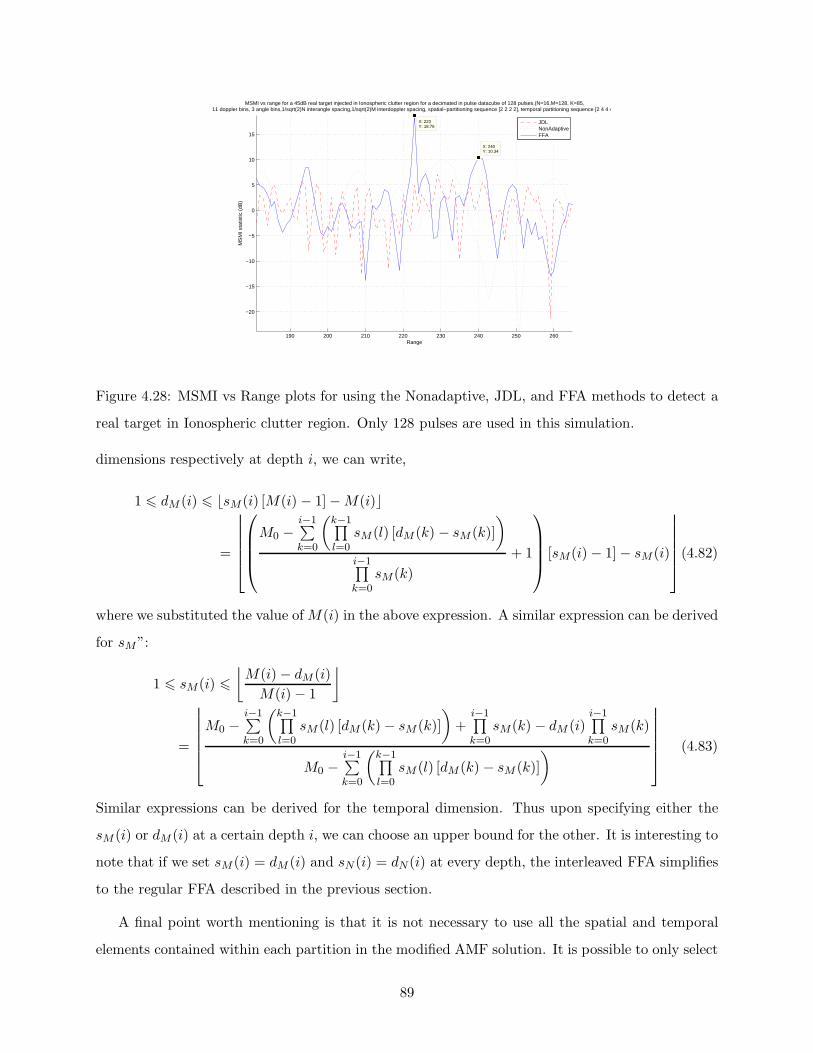
190 200 210 220 230 240 250 260
−20
−15
−10
−5
0
5
10
15
X: 223Y: 18.76
Range
MS
MI s
tatis
tic (
dB)
MSMI vs range for a 45dB real target injected in Ionospheric clutter region for a decimated in pulse datacube of 128 pulses.(N=16,M=128, K=85,11 doppler bins, 3 angle bins,1/sqrt(2)N interangle spacing,1/sqrt(2)M interdoppler spacing, spatial−partitioning sequence [2 2 2 2], temporal partitioning sequence [2 4 4 4])
X: 240Y: 10.34
JDLNonAdaptiveFFA
Figure 4.28: MSMI vs Range plots for using the Nonadaptive, JDL, and FFA methods to detect a
real target in Ionospheric clutter region. Only 128 pulses are used in this simulation.
dimensions respectively at depth i, we can write,
1 6 dM (i) 6 ⌊sM (i) [M(i) − 1] − M(i)⌋
=
M0 −i−1∑k=0
(k−1∏l=0
sM (l) [dM (k) − sM (k)]
)
i−1∏k=0
sM(k)
+ 1
[sM(i) − 1] − sM (i)
(4.82)
where we substituted the value of M(i) in the above expression. A similar expression can be derived
for sM”:
1 6 sM(i) 6
⌊M(i) − dM (i)
M(i) − 1
⌋
=
M0 −i−1∑k=0
(k−1∏l=0
sM (l) [dM (k) − sM (k)]
)+
i−1∏k=0
sM(k) − dM (i)i−1∏k=0
sM(k)
M0 −i−1∑k=0
(k−1∏l=0
sM (l) [dM (k) − sM (k)]
)
(4.83)
Similar expressions can be derived for the temporal dimension. Thus upon specifying either the
sM (i) or dM (i) at a certain depth i, we can choose an upper bound for the other. It is interesting to
note that if we set sM (i) = dM (i) and sN (i) = dN (i) at every depth, the interleaved FFA simplifies
to the regular FFA described in the previous section.
A final point worth mentioning is that it is not necessary to use all the spatial and temporal
elements contained within each partition in the modified AMF solution. It is possible to only select
89

Figure 4.29: A representation of the Interleaved-FFA method.
every kth spatial and every lth temporal element within each spatio-temporal partition. However
the same spatial and temporal sampling must be selected for all the partitions at the current depth.
Note that using fewer DoF per partition might lead to worse results than if all the DoF were used
since fewer DoF are harnessed towards suppressing the clutter and enhancing the target.
This new interleaved partitioning scheme is better than the original, since the different combi-
nations of DoF yield different intermediate statistics which better utilize the set of available DoF
at a certain depth to null the residual interference and enhance the buried target. Another ad-
vantage of the interleaved FFA is that this partitioning scheme can be used with values of M and
N that are prime or do not admit numerous factors. Unfortunately using interleaved partitions
further complicates the task of choosing an optimal spatio-temporal partition sequence, as we are
no longer bound to utilizing combinations of the factors of N and M , and the performance and
complexity is now determined by 4 parameter sequences (ignoring the available sample support K)
instead of only 2.
4.8 Complexity Analysis
Earlier we performed a complexity analysis on the regular FFA method and were able to derive
an expression for its asymptotic behavior. The interleaved FFA method’s complexity is somewhat
more difficult to characterize since it involves twice the number of parameters as the regular FFA
method. At a certain depth, i, and for the spatial and temporal partitions dN (i), sN (i), dM (i), and
90

sM (i) we must process M ′N ′ spatio temporal partitions using the modified AMF method, where,
M ′(i) =
⌊M(i) − dM (i)
sM(i)+ 1
⌋,
N ′(i) =
⌊N(i) − dN (i)
sN (i)+ 1
⌋.
(4.84)
The AMF solution requires the inversion of an M ′N ′ × M ′N ′ matrix, which is O((M ′N ′)3). Thus
the complexity of the interleaved FFA method can be shown to be,
Tint FFA =
max(kN ,kM)∑
i=1
{N ′(i)M ′(i)O((dN (i)dM (i))3)
}
=
max(kN ,kM )∑
i=1
{⌊N(i) − dN (i)
sN (i)+ 1
⌋⌊M(i) − dM (i)
sM (i)+ 1
⌋O((dN (i)dM (i))3)
},
(4.85)
where the value of M(i) is given in Eqn. (4.80), and that of N(i) can be inferred from Eqn. (4.80).
This expression compares to
TFFA =
max(kN ,kM )∑
d=1
NMd∏
i=1nimi
O((ndmd)
3)
=
max(kN ,kM )∑
d=1
{(max(kN ,kM )∏
i=d
nimi
)O((ndmd)
2)}
,
(4.86)
for the original FFA algorithm.
As can be seen by comparing the expressions outlining the complexities of the two algorithms
being evaluated, it is not straight forward to draw a definite conclusion. We can manipulate the
various parameters of each algorithm to favor either algorithm, in terms of complexity. However
the performance is directly related to the parameters and is often characterized by an inverse
relationship with the complexity, and therefore a tradeoff is inevitable. In general, in terms of
computation load, JDL has the distinct advantage that it requires the solution of single size-ηaηd
matrix while the FFA approach (in both its versions) requires several AMF solutions. On the other
hand, in terms of performance, the regular FFA algorithm uses all NM adaptive DoF while the JDL
is restricted to just ηaηd DoF. The interleaved FFA method goes beyond the regular FFA method
and reuses the DoF at each depth in the computation of intermediate statistics, and outperforms
the regular FFA method for a reasonably good choice of partitioning sequences.
4.8.1 Unequal Partitions
So far we have assumed that the partitions at each depth are of equal size, i.e., all the spatio-
temporal ’rectangles’ at a certain depth are of equal dimensions. Although this might seem neces-
91

sary so as to be able to express all the partial steering matrices at a given level in terms of the first
partial steering matrix at this level, we will show that this requirement can be easily bypassed by
using steering vectors that do not have constant phase progressions from element to element and/or
pulse to pulse. We will begin by assuming unequal but disjoint spatial and temporal partitions.
Starting with the original data-square of dimension N × M at a given look range we segment the
spatial and temporal dimensions into N1 and M1 unequal partitions respectively. We only require
that each of the spatial and temporal partitions be disjoint in order to simplify the presentation.
We can surely use an interleaved partitioning scheme as described in the previous section to bypass
the disjoint partitions requirement as well as use unequal partition sizes at any given depth of the
FFA tree structure. For the time being, however, we will assume disjoint partitions so as to avoid
overcomplicating an inherently simple idea. As a result we we will partition the spatial dimen-
sion into N1 disjoint partitions of lengths{
n(1)1 , n
(1)2 , . . . , n
(1)N1
}where,
N1∑l=1
n(1)l = N0. Similarly, we
will partition the temporal dimension into M1 disjoint partitions of lengths{m
(1)1 ,m
(1)2 , . . . ,m
(1)M1
}
where,M1∑k=1
m(1)k = M0.
Denote as X(1)lk and V
(1)lk the (l, k)-th spatio-temporal partition of the space-time snapshot
and steering matrix at the current depth respectively. Here l = 1, 2, .., N1 and k = 1, 2, ..,M1 .
We next process each spatio-temporal partition in a similar manner to the regular FFA method,
except instead of dividing by(w
(1)lk
)Hv
(1)11 where v
(1)11 is the actual first space-time partition of the
steering vector at the current depth, we replace v(1)11 by the vectorized form of a steering matrix
partition of dimension n(1)l ×m
(1)k whose first entry coincides with the first entry of the space-time
steering matrix of the current depth. We will denote this improvised steering matrix partition as
V(1)11 (n
(1)l ,m
(1)k ). Thus the expression for the (l, k)’th statistic evaluated from the (l, k)th spatio-
temporal data partition would be given by
y(1)lk =
(w
(1)lk
)Hx
(1)11
(w
(1)lk
)Hv
(1)11 (n
(1)l ,m
(1)k )
=
(w
(1)lk
)H (noise
(1)11 + clutter
(1)11
)
(w
(1)lk
)Hv
(1)11 (n
(1)l ,m
(1)k )
+
(w
(1)lk
)H (ξv
(1)lk
)
(w
(1)lk
)Hv
(1)11 (n
(1)l ,m
(1)k )
,
= s(1)lk + ξp
(1)lk ,
(4.87)
where,
p(1)lk =
(w
(1)lk
)Hv(1)lk
(w
(1)lk
)Hv
(1)11 (n
(1)l ,m
(1)k )
. (4.88)
is the (l, k)’th entry of the next depth’s spatio-temporal steering matrix. Thus by updating the
92

steering matrix at each depth we are not forced to rely on a preservation of a linear phase shift
throughout the depth of the FFA-tree structure. In fact the steering matrix need not be charac-
terized by any phase relationship amongst its entries; it suffices to know the form of the steering
matrix at any given depth in order to be able to perform the FFA processing at that depth. Actu-
ally this is also true for the AMF method which does not impose a particular form that should be
strictly adhered to by the steering matrix. The only strict requirement is that the steering matrix
be known apriori so that it may be used in the computation of the weight vector.
Thus it is possible to use unequal partition sizes at each depth, and still be able to perform FFA
processing. A further generalization of the FFA scheme is the combination of unequal partition sizes
at every depth with the use of interleaved sequences. This generalized form of the FFA could prove
to be very powerful, as it no longer requires N and M to be integers with numerous factors, and it
allows the possibility of DoF ’recycling’ which improves the detection capability of the algorithm.
A final yet very interesting thing to note, is that since we are not bound by any phase preser-
vation rule we need not divide by(w
(1)lk
)Hv
(1)11 to preserve a constant phase shift from element to
element after each processing stage. In fact we do not even need to use rectangular partitions. We
can simply choose any number of space-time elements at any random position in the current data-
square and subject them to a modified AMF processing. The resulting statistics can be grouped
into a new ‘data-square’ and reprocessed again in the forthcoming stage. Since we are free to choose
as many combinations of space-time elements to process at a given depth, we can end up with the
same, fewer , or more, number of elements at the next stage. As a result the method looses the
FFT like structure that originally inspired its development. In fact this method has no structural
pattern and becomes increasingly difficult to analyze. There are literally an infinite number of
ways to process a given cube using this unstructured method, and one can no longer think in the
direction of optimization. A practical implementation might rely on randomly choosing H bundles
of elements at every stage, performing the modified AMF on each bundle, then regrouping the
resulting statistics into a new vector. The sizes of each bundle could be chosen in such a way as
to yield decreasing subsequent vector sizes until a final statistic has been obtained. The ∆MSMIs
could then be tested for, and if the results are unsatisfying, the processing could be repeated using
a different choice of bundle sizes and/or element-bundle mappings. Another possibility would be
to repeat the above processing for a variety of element-bundle mappings, and averaging the final
statistic.
93
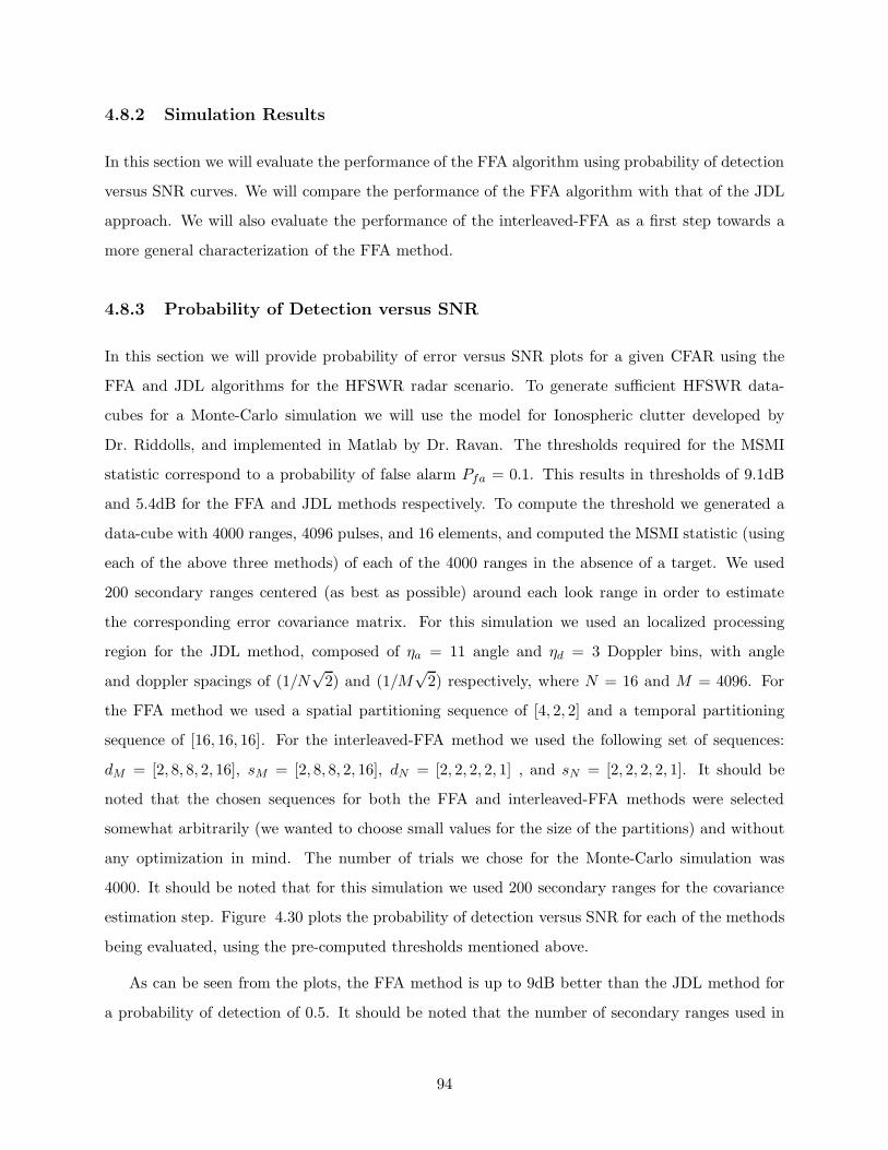
4.8.2 Simulation Results
In this section we will evaluate the performance of the FFA algorithm using probability of detection
versus SNR curves. We will compare the performance of the FFA algorithm with that of the JDL
approach. We will also evaluate the performance of the interleaved-FFA as a first step towards a
more general characterization of the FFA method.
4.8.3 Probability of Detection versus SNR
In this section we will provide probability of error versus SNR plots for a given CFAR using the
FFA and JDL algorithms for the HFSWR radar scenario. To generate sufficient HFSWR data-
cubes for a Monte-Carlo simulation we will use the model for Ionospheric clutter developed by
Dr. Riddolls, and implemented in Matlab by Dr. Ravan. The thresholds required for the MSMI
statistic correspond to a probability of false alarm Pfa = 0.1. This results in thresholds of 9.1dB
and 5.4dB for the FFA and JDL methods respectively. To compute the threshold we generated a
data-cube with 4000 ranges, 4096 pulses, and 16 elements, and computed the MSMI statistic (using
each of the above three methods) of each of the 4000 ranges in the absence of a target. We used
200 secondary ranges centered (as best as possible) around each look range in order to estimate
the corresponding error covariance matrix. For this simulation we used an localized processing
region for the JDL method, composed of ηa = 11 angle and ηd = 3 Doppler bins, with angle
and doppler spacings of (1/N√
2) and (1/M√
2) respectively, where N = 16 and M = 4096. For
the FFA method we used a spatial partitioning sequence of [4, 2, 2] and a temporal partitioning
sequence of [16, 16, 16]. For the interleaved-FFA method we used the following set of sequences:
dM = [2, 8, 8, 2, 16], sM = [2, 8, 8, 2, 16], dN = [2, 2, 2, 2, 1] , and sN = [2, 2, 2, 2, 1]. It should be
noted that the chosen sequences for both the FFA and interleaved-FFA methods were selected
somewhat arbitrarily (we wanted to choose small values for the size of the partitions) and without
any optimization in mind. The number of trials we chose for the Monte-Carlo simulation was
4000. It should be noted that for this simulation we used 200 secondary ranges for the covariance
estimation step. Figure 4.30 plots the probability of detection versus SNR for each of the methods
being evaluated, using the pre-computed thresholds mentioned above.
As can be seen from the plots, the FFA method is up to 9dB better than the JDL method for
a probability of detection of 0.5. It should be noted that the number of secondary ranges used in
94

25 30 35 40 45 50 55 60 65 70 75
0.2
0.3
0.4
0.5
0.6
0.7
0.8
0.9
1
X: 32Y: 0.146
HFSWR: Pd vs SNR using generated data−cubes (PFA=0.1).
SNR (dB)
Pd
FFAJDL
Figure 4.30: Probability of detection versus SNR for a PFA=0.1, using JDL, regular FFA, and
interleaved FFA methods.
this simulation is by far smaller than the required 2MN secondary samples required by the RMB
rule for optimal AMF performance. Unfortunately, given the time required, a corresponding plot
for the interleaved-FFA could not be obtained.
For completeness we will also evaluate the performance of the interleaved-FFA method (for the
chosen set of sequences) in the case of measured HFSWR data using both ideal and real targets.
Figures 4.31 and 4.32 show a ∆MSMI versus range plot for the interleaved-FFA methods in both
ideal and real target scenarios. As can be noted from the two figures, the interleaved-FFA method
outperforms the regular FFA method by approximately 3.5dB in the ideal target case and by 5.4dB
in the real target case. We repeat the above simulations for a reduced DoF scenario where only
128 of the available 4096 pulses are used (after appropriate decimation in pulse). In this simulation
we use a spatial-partitioning sequence of [2, 2, 2, 2] and temporal-partitioning sequence of [2, 4, 4, 4]
for the regular FFA method, and the following set of sequences for the interleaved-FFA method:
dM = [2, 34, 16, 1], sM = [2, 2, 13, 1], dN = [2, 5, 3, 2] , and sN = [2, 1, 1, 2] due to low sample
support (only 80 secondary samples used). We also use a spatial sampling sequence of [1, 2, 1, 1],
and a temporal sampling sequence of [1, 21, 2, 1]. The results for both ideal and real targets are
shown in Figures 4.33 and 4.34 respectively, where it can be seen that the interleaved-FFA method
is able to discriminate the 45dB ideal (real) targets with a margin of 8dB (7dB) over the regular
FFA method. As noted in an earlier report, the 45dB does not indicate the target signal-to-noise
ratio.
95

180 190 200 210 220 230 240 250 260 270
−20
−10
0
10
20
30
X: 176Y: 12.62
MSMI vs Range using a 45dB ideal target for regular, and interleaved−FFA.(N=16,M=4096,dN−sequence=[2 2 2 2 1],stepN−sequence=[1 1 1 1 1],sN−sequence=[2 2 2 2 1],dM−sequence=[2 8 8 2 16],stepM−sequence=[1 1 1 1 1],sM−sequence=[2 8 8 2 16],K=92)
X: 223Y: 35.11
X: 183Y: 8.574
X: 223Y: 34.49
interleaved−FFAFFA
Figure 4.31: MSMI versus range plot for interleaved-FFA method using 4096 pulses in an ideal
target scenario
180 190 200 210 220 230 240 250 260
−25
−20
−15
−10
−5
0
5
10
15
20
MSMI vs Range using a 45dB ideal target for regular, and interleaved FFA methods.(N=16,M=4096,dN−sequence=[2 2 2 2 1],stepN−sequence=[1 1 1 1 1],sN−sequence=[2 2 2 2 1],dM−sequence=[2 8 8 2 16],stepM−sequence=[1 1 1 1 1],sM−sequence=[2 8 8 2 16],K=80)
interleaved−FFAFFA
Figure 4.32: MSMI versus range plot for interleaved-FFA method using 4096 pulses in a real target
scenario
96
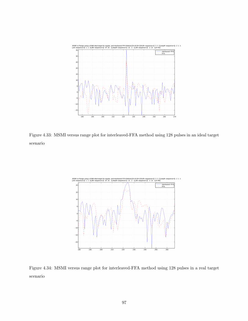
180 190 200 210 220 230 240 250 260 270
−15
−10
−5
0
5
10
15
20
25
30
35
MSMI vs Range using a 45dB ideal target for regular, and interleaved FFA Method.(N=16,M=128,dN−sequence=[2 5 3 2],stepN−sequence=[1 2 1 1],sN−sequence=[2 1 1 2],dM−sequence=[2 34 16 1],stepM−sequence=[1 21 2 1],sM−sequence=[2 2 13 1],K=92)
interleaved−FFAFFA
Figure 4.33: MSMI versus range plot for interleaved-FFA method using 128 pulses in an ideal target
scenario
180 190 200 210 220 230 240 250 260
−20
−15
−10
−5
0
5
10
15
20
MSMI vs Range using a 45dB ideal target for regular, and interleaved FFA Method.(N=16,M=128,dN−sequence=[2 5 3 2],stepN−sequence=[1 2 1 1],sN−sequence=[2 1 1 2],dM−sequence=[2 34 16 1],stepM−sequence=[1 21 2 1],sM−sequence=[2 2 13 1],K=80)
interleaved−FFAFFA
Figure 4.34: MSMI versus range plot for interleaved-FFA method using 128 pulses in a real target
scenario
97
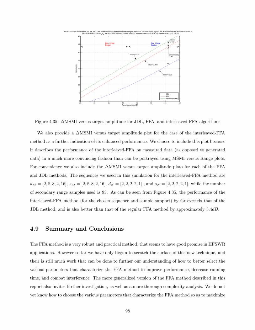
25 30 35 40 45 50 55 600
5
10
15
20
25
30
35
40
∆MSMI vs Target Amplitude for the JDL, FFA, and interleaved−FFA methods from ideal targets injected in the Ionospheric region of the HFSWR datacube using 18 iterations per SNR.(N=16, M=4096, K=93, (η
a,η
d, ∆a, ∆f) =(3,11,1/(N*sqrt(2)),1/(M*sqrt(2))), temporal−spacing=[4 4 16 16] , spatial−spacing=[2 2 2 2] )
Target Amplitude(dB)
∆MS
MI(
dB)
JDLFFAinterleaved−FFA
Non−LinearRegion
Non−LinearRegion
approximately11dB
slope=1.003
slope=1.006
slope=0.953
approx3.4dB
Figure 4.35: ∆MSMI versus target amplitude for JDL, FFA, and interleaved-FFA algorithms
We also provide a ∆MSMI versus target amplitude plot for the case of the interleaved-FFA
method as a further indication of its enhanced performance. We choose to include this plot because
it describes the performance of the interleaved-FFA on measured data (as opposed to generated
data) in a much more convincing fashion than can be portrayed using MSMI versus Range plots.
For convenience we also include the ∆MSMI versus target amplitude plots for each of the FFA
and JDL methods. The sequences we used in this simulation for the interleaved-FFA method are
dM = [2, 8, 8, 2, 16], sM = [2, 8, 8, 2, 16], dN = [2, 2, 2, 2, 1] , and sN = [2, 2, 2, 2, 1], while the number
of secondary range samples used is 93. As can be seen from Figure 4.35, the performance of the
interleaved-FFA method (for the chosen sequence and sample support) by far exceeds that of the
JDL method, and is also better than that of the regular FFA method by approximately 3.4dB.
4.9 Summary and Conclusions
The FFA method is a very robust and practical method, that seems to have good promise in HFSWR
applications. However so far we have only begun to scratch the surface of this new technique, and
their is still much work that can be done to further our understanding of how to better select the
various parameters that characterize the FFA method to improve performance, decrease running
time, and combat interference. The more generalized version of the FFA method described in this
report also invites further investigation, as well as a more thorough complexity analysis. We do not
yet know how to choose the various parameters that characterize the FFA method so as to maximize
98
it performance, nor do we fully understand how these parameters impact target discrimination and
clutter mitigation. A more elaborate investigation of the FFA technique is necessary before the full
picture portrayed by this elegant method can be seen.
In this section we introduced a generalized form of the FFA method introduced in Section 4.6.
We also used the new Ionospheric clutter model developed by Dr. Riddolls to generate HFSWR
datacubes corrupted by Ionospheric clutter, which we required to generate probability of detection
versus SNR plots that better characterize the performance of the FFA method. We also provided
a ∆MSMI versus target amplitude plots for the interleaved-FFA method and used it to further
describe the performance of this more general version of the FFA as applied to measured HFSWR.
99
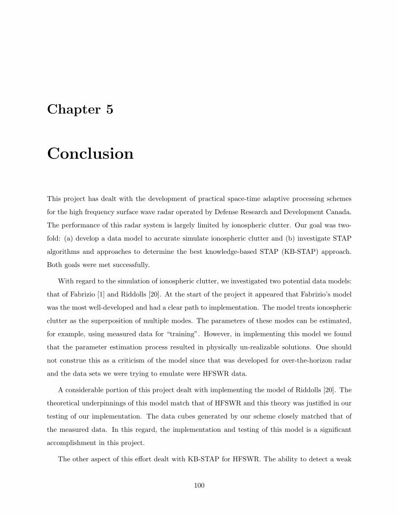
Chapter 5
Conclusion
This project has dealt with the development of practical space-time adaptive processing schemes
for the high frequency surface wave radar operated by Defense Research and Development Canada.
The performance of this radar system is largely limited by ionospheric clutter. Our goal was two-
fold: (a) develop a data model to accurate simulate ionospheric clutter and (b) investigate STAP
algorithms and approaches to determine the best knowledge-based STAP (KB-STAP) approach.
Both goals were met successfully.
With regard to the simulation of ionospheric clutter, we investigated two potential data models:
that of Fabrizio [1] and Riddolls [20]. At the start of the project it appeared that Fabrizio’s model
was the most well-developed and had a clear path to implementation. The model treats ionospheric
clutter as the superposition of multiple modes. The parameters of these modes can be estimated,
for example, using measured data for “training”. However, in implementing this model we found
that the parameter estimation process resulted in physically un-realizable solutions. One should
not construe this as a criticism of the model since that was developed for over-the-horizon radar
and the data sets we were trying to emulate were HFSWR data.
A considerable portion of this project dealt with implementing the model of Riddolls [20]. The
theoretical underpinnings of this model match that of HFSWR and this theory was justified in our
testing of our implementation. The data cubes generated by our scheme closely matched that of
the measured data. In this regard, the implementation and testing of this model is a significant
accomplishment in this project.
The other aspect of this effort dealt with KB-STAP for HFSWR. The ability to detect a weak
100

target is largely restricted by the ionospheric clutter. The HFSWR data sets are characterized by
the very large available degrees of freedom (M = 4096 pulses, N =16 elements) and the extremely
restricted available training data (approximately 80 range cells in total including oversampled
range cells). Our initial effort, therefore, was focused on the implementation and testing of popular
reduced DoF algorithms (with attendant reductions in required training). We implemented and
tested the joint domain localized (JDL), direct data domain (D3), hybrid and parametric adaptive
matched filter (PAMF) schemes. The JDL and hybrid schemes were considered the most promising.
The continued investigation of these schemes was superseded by the development of a new space-
time adaptive processing scheme: the fast fully adaptive (FFA) algorithm. This scheme draws its
inspiration from the popular FFT scheme - the overall fully adaptive scheme that uses all NM
DoF is sub-divided into a a nested process of significantly smaller “fully” adaptive problems. At
each level, only limited secondary training samples are required but the overall solution exploits all
available DoF.
In this report we have detailed the FFA algorithm and its variants, the interleaved FFA scheme
and a general scheme with potentially unequal spacings. The performance of these schemes are
documented using the measured data and the simulated data as described above.
101

Bibliography
[1] G. Fabrizio, “Space-time characterization and adaptive processing of ionospherically propa-
gated hf signals,” Ph.D. dissertation, The University of Adelaide,, 2000.
[2] R. J. Riddolls, “a model of radio wave propagation in ionospheric irregularities for prediction
of high-frequency radar performance,” Defense Research Development Canada - Ottawa, Tech.
Rep. TM 2006-284, December 2006.
[3] M. Ravan, O. Saleh, R. Adve, and K. Plataniotis, “KB-STAP implementaion for HFSWR:
Progress report,” Tech. Rep. W7714-060999/001/SV, June 2007.
[4] ——, “KB-STAP implementaion for HFSWR: Progress report,” Tech. Rep. W7714-
060999/001/SV, September 2007.
[5] R. S. Adve, T. B. Hale, M. C. Wicks, and P. A. Antonik, “Ground moving target indica-
tion using knowledge based space-time adaptive processing,” in Proceedings of the 2000 IEEE
International Radar Conference, May 2000, washington, DC.
[6] R. S. Adve, T. B. Hale, and M. C. Wicks, “Knowledge based adaptive processing for ground
moving target indication,” DSP: A Review Journal, available on-line August 2005. Also avail-
able at http://www.comm.utoronto.ca/ rsadve/publications.html.
[7] ——, “Joint domain localized adaptive processing in homogeneous and non-homogeneous en-
vironments. part II: Non-homogeneous environments,” IEE Proceedings on Radar Sonar and
Navigation, vol. 147, no. 2, pp. 66–73, April 2000.
[8] R. Adve, P. Missailidis, and K. Plataniotis, “KB-STAP implementaion for HFSWR: Progress
report,” Tech. Rep. W7714-060999/001/SV, March 2007.
102
[9] H. Wang and L. Cai, “On adaptive spatial-temporal processing for airborne surveillance radar
systems,” IEEE Transactions on Aerospace and Electronic Systems, vol. 30, no. 3, pp. 660–699,
July 1994.
[10] R. S. Adve, T. B. Hale, and M. C. Wicks, “Joint domain localized adaptive processing in
homogeneous and non-homogeneous environments. part I: Homogeneous environments,” IEE
Proceedings on Radar Sonar and Navigation, vol. 147, no. 2, pp. 57–65, April 2000.
[11] M. Ravan, O. Saleh, R. Adve, and K. Plataniotis, “KB-STAP implementaion for HFSWR:
Progress report,” Tech. Rep. W7714-060999/001/SV, December 2007.
[12] J. W. X. Kun Lu, “A piecewise parametric method based on polynomial phase model to com-
pensate ionospheric phase contamination,” IEE Proceedings on Radar, Sonar and Navigation,
2003.
[13] K. Lu, X. Liu, and Y. Liu, “A multiple-Sweep-Frequencies Scheme Based on Eigen-
decomposition to Compensate Ionospheric Phase Contamination,” in Proceedings of the 2003
IEEE International Radar Conference, September 2003, pp. 706–710.
[14] A. Bourdillon, “Use of of maximum entropy spectral analysis to improve ship detection by
over-the-horizon radar,” Radio Science, vol. 22, no. 2, pp. 313–320, 1987.
[15] J. Parent and A. Bourdillon, “A method to correct hf sky-wave backscattered signals for
ionosphere frequency modulation,” IEEE Transactions on Antennas and Propagation, vol. 36,
no. 1, pp. 127–135, 1988.
[16] Y. Abramovich, S. Anderson, and Soloman, “Adaptive ionospheric distortion correction tech-
niques for HF sky-wave radar,” in Proceedings of the 1994 IEEE National Radar Conference,
1994.
[17] M. D. M. Paul D. Mountcastle, “Monte-carlo simulation of ionospheric scintillation,” in Pro-
ceedings of the 2002 IEEE Radar Conference, 2002.
[18] C. J. Coleman, “A model of HF sky wave radar clutter,” Radio Science, vol. 31, no. 4, pp.
869–876, August 1996.
[19] ——, “A propagation model for HF radiowave systems,” in Conference Record of the 1994
IEEE Military Communications Conference, 1994, vol. 3, October 1994, pp. 875–879.
103

[20] R. J. Riddolls, “A model of radio wave propagation in ionospheric irregularities for prediction
of high-frequency radar performance,” Defense Research Devlopment Canada - Ottawa, Tech.
Rep. DRDC Ottawa TM 2006-284, December 2006.
[21] R. Riddolls, “Measurement of ionospheric density irregularity spectra for evaluation of next-
generation OTH radar systems,” in Proceedings of the 2007 Union of Radio Science Interna-
tional Conference, July 2007.
[22] H. C. Chan, “Characterization of ionospheric clutter in HF surface-wave radar,” Defense Re-
search Devlopment Canada - Ottawa, Tech. Rep. DRDC Ottawa TR 2003-114, September
2003.
[23] L. Sevgi, A. Ronsford, and H. C. Chan, “An integrated maritime surveillance system based
on high-frequency surface wave radars, part 1: Theoretical background and numerical simula-
tions,” IEEE Antennas and Propagation Magzine, vol. 43, no. 4, pp. 28–42, 2001.
[24] ——, “An integrated maritime surveillance system based on high-frequency surface wave
radars, part 2: Operational status and system performance,” IEEE Antennas and Propagation
Magzine, vol. 43, no. 4, pp. 52–63, 2001.
[25] L. Sevgi, “Stochasting modelling of target detection and tracking in surface wave radar,”
International Journal of Numerical Modelling, vol. 11, no. 3, pp. 168–181, 1998.
[26] R. H. Anderson and J. L. Krolik, “Track association for over-the-horizon radar with a statistical
ionospheric model,” IEEE TRANSACTIONS ON SIGNAL PROCESSING, vol. 50, no. 11, pp.
2632–2643, November 2002.
[27] H. Leong, “Adaptive nulling of skywave interference using horizontal dopole antennas in a
coastal surveillance HF surfave wave radar system,” Defense Research Establishment Ottawa,
Tech. Rep. 506722 (System Number), June 1997.
[28] ——, “Adaptive suppression of interference in HF surfave wave radar using auxiliary horizontal
dopole antennas,” Defense Research Establishment Ottawa, Tech. Rep. 1336 (Report Number),
Sept. 1998.
[29] ——, “A comparison of sidelobe cancellation techniques using auxiliary horizontal and vertical
antennas in HF surface wave radar,” Defense Research Establishment Ottawa, Tech. Rep.
DREO TM 1999-121, November 1999.
104

[30] H. C. Chan and E. K. L. Tung, “An investigation in interference suppression in HF surface wave
radar,” Defense Research Establishment Ottawa, Tech. Rep. DREO TR 2000-028, December
1999.
[31] Y. Abramovich, S. Anderson, Y. Lyudviga, N. Spencer, P. Turcaj, and B. Hibble, “Space-time
adaptive techniques for ionospheric clutter mitigation in HF surface wave radar systems,” in
Proceedings of the 2004 IEEE International Radar Conference, 2004.
[32] G. A. Fabrizio, A. Farina, and M. Turley, “Spatial adaptive subspace detection in OTH radar,”
IEEE Transactions on Aerospace and Electronic Systems, vol. 39, no. 4, pp. 1407–1427, 2003.
[33] G. A. Fabrizio, L. L. Scharf, A. Farina, and M. Turley, “Ship detection with HF surface wave
radar using short integration times,” in Proceedings of the 2004 IEEE International Radar
Conference, 2007.
[34] G. A. Fabrizio, G. J. Frazer, and M. Turley, “STAP for clutter and interference cancellation
in a HF radar system,” in Proceedings of ICASSP 2006, 2006.
[35] S. Kraut, L. L. Scharf, and T. McWhorter;, “Adaptive subspace detectors,” IEEE Transactions
on Signal Processing, vol. 49, no. 1, pp. 1–16, January 2001.
[36] G. A. Fabrizio and A. Farina, “GLRT-based adaptive processing for HF radar systems,” in
Proceedings of the 2007 IEEE Radar Conference, 2007.
[37] G. Li, L. Li, and R. Xu, “A novel adaptive beamforming method for non-stationary interference
cancellation in HF surface wave radar,” in Proceedings of the 2004 IEEE International Radar
Conference, 2004.
[38] W. Xianrong, K. Hengyu, and W. Biyang, “Adaptive cochannel interference suppression based
on subarrays for HFSWR,” IEEE Signal Processing Letters, vol. 12, no. 2, pp. 162–165, Feb.
2005.
[39] W. Xianrong, C. Feng, and K. Hengyu, “Experimental trials on ionospheric clutter suppression
for high-frequency surface wave radar,” IEE Proceedings on Radar, Sonar and Navigation, vol.
153, no. 1, pp. 23–29, Feb. 2006.
[40] K. Lu and X. Liu, “STAP for clutter and interference cancellation in a HF radar system,” in
Proceedings of ICASSP 2004, 2004.
105
[41] K. Lu, X. Liu, and Y. Liu, “Ionospheric decontamination and sea clutter suppression for HF
skywave Radars,” IEEE Journal of Oceanic Engineering, vol. 30, no. 2, pp. 455–462, April
2005.
[42] A. Bourdillon, P. Dorey, and G. Auffray, “Ship echo discrimination in HF radar sea-clutter,”
in Proceedings of the 2003 IEEE International Radar Conference, 2003, pp. 584–587.
[43] S. Kraut, K.Harmanci, and J. Krolik, “Space-time adaptive processing for over-the-horizon
spread-doppler clutter mitigation,” in Proceedings of the SAM signal Processing Workshop,
2000.
[44] J. Ward, “Space-time adaptive processing for airborne radar,” MIT Linclon Laboratory, Tech.
Rep. F19628-95-C-0002, December 1994.
[45] I. S. Reed, J. Mallett, and L. Brennan, “Rapid convergence rate in adaptive arrays,” IEEE
Transactions on Aerospace and Electronic Systems, vol. 10, No. 6, pp. 853–863, Nov. 1974.
[46] L. Cai and H. Wang, “Performance comparisons of modified SMI and GLR algorithms,” IEEE
Transactions on Aerospace and Electronic Systems, vol. 27, no. 2, pp. 487–491, Apr. 1991.
[47] Y. Abramovich, A. Ghorokhov, and C. Demeure, “Adaptive verification of a general multi-
variate propagation model for ionospheric hf signals,” in Proceedings of the 1996 EUSIPCO,
1996.
[48] T. K. Sarkar and N. Sangruji, “An adaptive nulling system for a narrow-band signal with
a look-direction constraint utilizing the conjugate gradient method,” IEEE Transactions on
Antennas and Propagation, vol. 37, no. 7, pp. 940–944, July 1989.
[49] J. Roman, M. Rangaswamy, D. Davis, Q. Zhang, B.Himed, and J. Michels, “Parametric adap-
tive matched filter for airborne radar applications,” IEEE Transactions on Aerospace and
Electronic Systems, vol. 36, No. 2, pp. 677–692, 2000.
[50] J. Goldstein, L. Scharf, and I. Reed, “A multistage representation of the wiener filter based
on orthogonal projections,” IEEE Transactions on Information Theory, vol. 44, no. 7, pp.
2943–2959, July 1998.
[51] E. Yang, J. Chun, and R. Adve, “A hybrid d3-sigma delta stap algorithm in non-homogeneous
clutter,” To appear, IEEE International Radar Conf., October 2007.
106

[52] S. Marple, Digital Spectral Analysis with Applications. Prentice Hall, 1987.
107