FreightBestPractice

Key Performance Indicators forFood and Drink Supply Chains

November 2007.

Printed in the UK on paper containing at least 75% recycled fibre.

FBP1086 # Queens Printer and Controller of HMSO 2007.

BenchmarkingGuide

Acknowledgements

Thanks are due to the following businesses which took part in the Survey. The time and effort put in by their staff in

attending workshops and gathering data is greatly appreciated.

Drinks

BargainBooze

Carlsberg

CERT Group

Daniel Thwaites Brewery

Everards Brewery

Hall & Woodhouse

Heineken

Inbev UK

Kuehne & Nagel Drinks

Miller Brand

Shepherd Neame

Wincanton

Food

3663

Allied Bakeries

Asda

Booker

Boughey Distribution

Christian Salvesen

Cold Move

Co-operative Retail

Dairy Crest

Elddis Transport

Fox’s Biscuits

GIST

Gregory Distribution Ltd

Kuehne &Nagel Food

Langdons

Wm Morrison Supermarkets Ltd

Nestle UK

NFT Distribution

Re-Vision Logistics/Nisa Today

Sainsburys

Samworth Brothers Distribution

Somerfield

Tesco

Tetley Tea

Thorntons

United Biscuits

Walkers Crisps

i

Contents

Foreword iv

1 Introduction 1

2 The Key Performance Indicators 2

2.1 Survey Statistics 3

2.2 The Survey Data 4

2.3 Vehicle Fill 4

2.4 Empty Running 6

2.5 Time Utilisation 7

2.6 Deviations from Schedule (Delays) 10

2.7 Fuel Consumption and Energy Efficiency 12

2.8 Operating Instructions 14

3 Conclusions 15

3.1 Levels of Efficiency 15

3.2 Utilisation over 24 hours and 7 days 16

3.3 Summary 16

Glossary of Terms 18

iii

Foreword

The role of Key Performance Indicators is well known

and established throughout all sectors of industry.

They provide a simple, focussed measure of

performance, and so provide management with a

short, concise picture of what is happening in their

operation.

Over the past few years, the Department for Transport,

through the Freight Best Practice programme, has

supported a number of surveys that have developed a

range of Key Performance Indicators (KPIs) in a

variety of industry sectors.

The KPIs have provided those in the freight industry

with a consistent measure of the levels of efficiency

being achieved within their sector. Comparing, or

benchmarking, their own performance against those

KPIs provides the opportunity to focus on those

aspects which are most likely to yield performance

improvement.

This Benchmarking Guide aims to provide operators

with those critical comparisons, and hence to help

them improve efficiency, reduce operating costs and to

reduce the impact of road transport on the

environment.

iv

1 Introduction

As far back as 1992 the Department of the

Environment supported a project on improving vehicle

aerodynamics through the Energy Efficiency Best

Practice programme. This was followed by the

establishment of a discrete transport efficiency

programme in 1994, which by 2005 had evolved into

the Freight Best Practice Programme.

The first substantial survey in the food sector was

carried out in 1998, followed by a much larger survey in

2002. The results enabled participants to benchmark

their individual performance against companies within

their sector.

The 2007 Survey is a natural progression in a line of

similar work all aimed at providing operators with

accurate, reliable measures by which their own

performance can be compared with the results

achieved by others. For the first time the remit has

been extended to include the drinks sector, and there

is a commitment to carry out a further survey in 2009.

The overall aim of this Survey, and previous ones, was

to:

Provide measures of efficiency levels being

achieved in the food and drinks sectors

Enable companies to measure their own

efficiency against that of the industry as a whole

Stimulate and support existing efforts to improve

efficiency in the operation and use of vehicles.

For the 2007 Survey the activities of almost 9,000

vehicles - tractors units, trailers, and rigids - were

closely monitored and recorded. These vehicles were

operating in the food and drinks sectors, and covered

the movement of product from producers to the

ultimate point of sale. The data gathered enabled the

operational efficiency of those vehicles to be analysed,

and measures of that efficiency, i.e. Key Performance

Indicators were established.

Comparisons with previous surveys will show general

trends and highlight the way that the supply process for

food has changed in the last decade or so. However,

there were differences in the fleet mix between 1998,

2002 and 2007, both at sector and sub-sector level,

and so it is impossible to be sure that the results

represent an absolute ‘like for like’ comparison.

The Survey gathered information in three broad

categories:

General information covering the details of the

vehicles being surveyed – size, type, capacity,

age, fuel consumption

Detailed data on a leg by leg basis, for all

journeys undertaken during the sample period

An audit of vehicle activity during the sample

period.

Previous Surveys have studied trailers, semi-trailers

and rigids, i.e. the load carrying elements. For this

Survey, activity information was also gathered on

tractor units.

In order to make the results as reliable as possible,

and, therefore, the most useful both to participants and

subsequent users of the Guide, it is important that data

gathering is carefully prescribed. Standard software

was used as the medium to assemble the information

and enable computer analysis.

Previous surveys had used a 48 hour sample period

but for 2007 it was decided that 24 hours was perfectly

adequate. The previous survey results – where they

provide a picture of activity across the sample period -

show that the first 24 hour period looked very similar to

the second. A reduction to 24 hours therefore imposed

less data gathering on participants without detracting

from the value of the results. However, in addition data

covering daily activity was also collected to

demonstrate day to day variations plus the impact of 7

day trading.

1

2 The Key PerformanceIndicators

The main KPIs used in the 2007 Survey were the same

as those used in the 2002 Survey. With due regard to

the caution expressed above about like-for-like

comparisons, this Survey does provide operational

measures which can now be traced back for almost ten

years.

The main KPIs were:

1. Vehicle Fill

This is the measure of load carried, compared with

vehicle capacity, on each loaded leg.

For the food sector this was done by payload weight,

load height and load unit numbers. In most loads in the

food Survey product was carried in unit loads, i.e. a roll

cage or wooden pallet. Where this was not the case

conversion factors were used to enable the creation of

a pallet-equivalent measure, and hence a deck fill

measure.

For the drinks vehicles participants were offered the

option of using tonnage – being the total weight of

kegs/cask and bottles of beers, wines spirits and soft

drinks, or a combination of the number of kegs/casks,

plus the number of pallets used to load bottled product.

2. Empty Running

This is the distance which a vehicle runs empty, that is

not carrying product, usually the final leg of a journey

when the vehicle returns to depot or moves on to

another point at which it collects a load.

3. Time Utilisation

This was the measure of what vehicles were doing

during each hour throughout the sample period. The

seven categories used were: running on the road,

awaiting loading/unloading, being loaded/unloaded,

pre-loaded and awaiting departure, driver daily

(‘overnight’) rest period, vehicle idle (empty and

stationary) and maintenance or repair.

Additionally, for tractor units only, there was ‘running

solo’ (i.e. without a semi-trailer).

4. Deviation from Schedule (Delays)

This is the measure of the delays suffered by the

vehicles in the Survey. Categories of delay were: lack

of driver, delay at vehicle’s own base/point of

departure, delay at a collection point, traffic delay,

vehicle breakdown.

5. Fuel consumption

Data was requested for each vehicle type within the

Survey. Performance over a sustained period was

required and so data covering three winter months was

requested.

The unit of measure used is miles per gallon, due to

operator feedback suggesting that mpg was still the

measure which people used most readily and could

relate to.

The Survey covered all aspects of the movement of

finished food, i.e. food that is ready for sale rather than

raw materials. Activities were separated into:

Primary: Movement of saleable product, raw

material, work in progress, returns, packaging or

handling equipment between a supplier and

factory/factory and NDC/NDC and customer’s

RDC, Hub depot or Wholesale depot including

C&Cs

Secondary: Movement of saleable product from

retailer RDC or Food Service Hub depot into

retail outlet or picking depot. In addition, the

return of equipment or goods from outlet to RDC

or Hub.

Tertiary: Movement of saleable goods from a

factory, regional or picking depot, including

wholesaler, into the final outlet where product is

consumed i.e. home, pubs & clubs, small

independent corner shops, retail forecourts or

restaurants

2

2.1 Survey Statistics

A total of 113 fleets, from both food and drinks sectors,

participated in the Survey, which now falls into the

category of a ‘devolved function’ and so only covers

fleets based in England, or operating mainly in England.

During the 24 hours the food sector vehicles delivered

over 147 thousand pallet equivalents, and those in the

drinks sector delivered 12,716 tonnes of product. Total

distance run for both groups of vehicles was almost 1.4

million kilometres.

Tables 1 and 2 show the Survey Statistics.

NB It should be remembered that the 1998 and 2002

Surveys covered two days and the 2007 Survey

covered only one.

Primary

Secondary

Tertiary

Production

Primary Consolidation Centre

Multiple retail outlet

Local W'sale/Cash & CarryWarehouse

Retail forecourt Catering outlet Independent retail outlet

National/RegionalDistribution Centre

(supermarket chain)

Regional Distribution Centre(large wholesaler)

Figure 1 Food Distribution Channels

Table 1 Survey Statistics – Food

1998 2002 2007

No. of fleets 36 53 91

Tractor Units 1,393 1,446 2,286

Trailers 1,952 3,088 4,052

Rigid vehicles 182 546 1,362

Journeys/24 hrs 2,012 3,034 7,064

Journey legs/24 hrs 5,937 12,222 23,044

Pallets delivered/24 hrs 103,101 110,329 147,645

Kilometres travelled/24hrs 580,956 727,111 1,226,408

Table 2 Survey Statistics - Drink

2007

No. of fleets 22

Tractor Units 363

Trailers 644

Rigid vehicles 268

Journeys 956

Journey legs 5,435

Tonnes delivered 12,716

Kilometres travelled 172,028

3

2.2 The Survey Day

Unlike previous Surveys the 2007 covered only a

single day. Activity on the sample day (Thursday)

compared with the remainder of the week is shown in

Figure 2.

2.3 Vehicle Fill

The measurement of vehicle capacity in the food

sector is relatively complex. Vehicles will either ‘weight

out’, i.e. the payload limit is reached, or, more usually,

they will ‘cube out’ i.e. the vehicle is filled before

reaching its allowed payload limit.

For this survey, as with the previous ones, the

fundamental unit used was the pallet, being regarded

as having dimensions of 1m by 1.2m. Where

companies used different handling methods – roll

cages, cartons, or dollies with tote boxes for instance –

the number of these carried was converted into pallet

equivalents, that is 1.2 square metres of vehicle deck

space. The survey also asked for tonnage carried and

for vehicle carrying capacity.

The second key measure was typical height of a load

within the vehicle. Participants were asked to provide

an estimate of the typical load height profile across

their operation.

The average height used on laden trips is shown below

in Figure 3

The results show that many companies are unable to

use the typical available height within a ‘standard’

vehicle of around 2.1 metres, which allows for air

circulation in temperature controlled vehicles. Across

all trips in the survey on the sample day, the mean

height utilisation figure was 72%.

Table 3 shows a considerable change in profile since

the 2002 survey, but the overall effect is a marginal

improvement in use of vehicle height of around 1%.

This appears to an opportunity for significant

improvement but there are a number of obstacles

which prevent using the cube. These include an

inability to stack certain products due to fragility or

instability, or a requirement to supply pallets of a

particular height to customers, or a customer

requirement for single stacking.

The average utilisation for each fleet is shown in

Figures 4 and 5.

Taking all food trips within the survey the average deck

utilisation, measured by use of deck space, was

74.8%, and by weight was 55.1%.

SatFriThuWedTueMon0%

5%

10%

15%

20%

25%

Sun

Food Drinks

Figure 2 Percentage of volume delivered across the week

40%35%30%25%20%15%10%5%

5%

28%

32%

35%

0%

less than 0.8mabove deck

between 0.8m and1.5m above deck

between 1.5m and1.7m above deck

over 1.7mabove deck

Figure 3 Distribution of heights on loaded vehicle trips (food)

Table 3 Vehicle Height Utilisation (food) %age of

trips by height utilised

2002 2007

under 0.8m 9% 5%

0.8 – 1.5m 9% 28%

1.5m – 1.7m 67% 32%

Over 1.7m 15% 35%

4

Across the three activity streams in food the levels of

utilisation, measured by each individual trip, were as

shown in Figure 6 below.

Utilisation of height within drinks fleets (Figure 7) is to a

large extent governed by methodology used. Many

dray operations carry kegs and casks loose within the

load, and so stacking, to any great extent, is not

practical. The primary fleets, delivering mainly into the

food retail and wholesale sectors can stack pallets of

canned or bottled drinks, and by the use of locator

boards, can also stack kegs and casks.

Within drinks the utilisation measure used is weight,

and Figure 8 shows the average weight utilisation for

each fleet.

In the case of drinks vehicles, particularly drays on

pub/club deliveries, most operators use tonnage

including keg/cask beer and bottled beers, wines,

spirits and soft drinks) as a measure of vehicle fill.

However, although kegs or casks are heavy, the

vehicles rarely use their full weight carrying capability.

Vehicle operators use a notional vehicle capacity, in

tonnes, for load planning, based on their experience of

what will fit onto vehicles. This notional capacity is

rarely, if ever, the same as the vehicle’s legal weight

carrying capacity, and there is often a difference of

several tonnes on a typical 17/18t vehicle. It is this

notional capacity figure on which the utilisation

calculations are made.

Due to the inherent difficulties of handling and

securing, kegs and casks are rarely stacked on drays

and so the load height is usually low.

0%

10%

20%

30%

40%

50%

60%

70%

80%

90%

100%

Fleets

Figure 4 Average deck utilisation by fleet (food)

0%

10%

20%

30%

40%

50%

60%

70%

80%

90%

100%

Fleets

Figure 5 Average weight utilisation by fleet (food)

MixedTertiarySecondaryPrimary0%

10%

20%

30%

40%

50%

60%

70%

80%

90%

Average

Area Fill

Weight Fill

Figure 6 Vehicle Utilisation by activity (food)

60%50%40%30%20%10%

13%

48%

39%

0%

less than 0.8mabove deck

between 0.8m and1.5m above deck

over 1.5mabove deck

Figure 7 Distribution of heights on loaded vehicle trips (drinks)

0%

10%

20%

30%

40%

50%

60%

70%

80%

90%

Fleets

Figure 8 Average weight utilisation by fleet (drinks)

5

2.4 Empty Running

Empty running is widely seen as the bane of

commercial vehicle operation since it usually

represents mileage which is being run without direct

commercial benefit or purpose, at best returning or

moving on to collect another load. There is a perception

amongst the public that lorries run half empty most of

the time, or completely empty for half of the time.

In fact, of the 1.39 million kilometres run by the

vehicles during the Survey, just 24.1% of food vehicle

kilometres were empty, while the corresponding

number for drinks was 20.1%. These are higher than

the 2002 figure of 19% but lower than the 27.4%

quoted in the Department for Transport’s Transport

Statistics Bulletin Road Transport 2005.

The question of empty running is made more

complicated in the food sector by the use by many

retailers of roll-cages for the inbound supply to their

stores. Having been delivered to stores with product

they must of course be returned to Distribution Centres

for re-filling. This return journey takes up a vehicle’s

load space, even when the roll-cage design allows the

cages to be nested when empty.

Since the cage is empty it can be argued that the

vehicle is also empty, since it carries no saleable

product, and that the carriage of empty roll-cages is the

result of the mode of delivery operation chosen by that

retailer. The alternative view is that a vehicle loaded

with empty roll-cages is full. Whatever the view, in

practice the carriage of empty roll cages takes up

space and prevents the carriage of other, usually

palletised goods, such as new product from a supplier.

The proportion of empty kilometres run, i.e. those

without any product, by each fleet carrying product in

cages or other containers is shown in Figure 9.

For comparison, Figure 10 shows the proportion of

empty running incurred by fleets which deliver on

pallets rather than in cages.

In fact the proportion of empty running carried out by

vehicles carrying product in cages is very similar to

those carrying product on pallets. In the case of the

cage carrying vehicles however there is less scope to

carry backloads because of the volume taken up by

cages.

Empty running is an inevitable part of vehicle operation

in the food sector and the extent of it is dependant on

both the nature of the journey – primary, secondary or

tertiary – and on the way that vehicle delivery routes

are planned and executed.

A primary route may involve a full load delivery to a

single point and then a return. If no arrangements for a

backload are, or can be, made then 50% empty

running will result.

A secondary or tertiary delivery route will usually run

the last leg empty, but the length of that last leg, and

hence the proportion of empty running can depend on

the way that the journey is planned. If deliveries are

done on the outbound part of the journey, up 50%

(returning mileage) may be empty, whereas running

out to the furthest point and offloading on the way back

may leave only a short empty leg back to base after the

last drop.

0%

10%

20%

30%

40%

50%

60%

average23.7%

Fleets

Figure 9 Proportion of kilometres run empty, by cage carrying

fleet (food)

0%

5%

10%

15%

20%

25%

30%

35%

40%

45%

50%

average24%

Fleets

Figure 10 Proportion of empty running by pallet carrying fleets

(food)

6

Table 4 gives the percentage of empty miles by activity

for the food sector.

In the case of the drinks sector the return of empty

kegs and casks is inevitable. They are the only means

of supplying draft beers and lagers and far too

expensive to be anything other than returnable. The

amount of empty running within drinks is less than in

food as shown below in Figure 11.

2.5 Time Utilisation

Vehicle activity over the 24 hour period was measured

by recording the main activity of each vehicle for each

hour of the Survey. Trailers and rigids in the food

sector spent 30% of the time running on the road

(Figure 12). This includes 2% on overnight breaks and

so is the same as the 2002 percentage.

Although vehicle operation is seen as being a

substantial expense the Survey shows that, in the food

sector, vehicles spend slightly less time (49%) active –

on the road, loading/unloading, or delayed – than they

do inactive.

The comparisons above clearly show the benefit of

using articulated combinations where the time spent on

the road by tractor units was 49% compared with just

30% for the group of vehicles as whole.

The figures for trailer and rigid activities in the drinks

sector are shown below.

Table 4 Empty running by activity (food)

Activity % of kms empty

Primary 23.9

Secondary 22.8

Tertiary 28.4

0%

5%

10%

15%

20%

25%

30%

35%

40%

average20.3%

Fleets

Figure 11 Proportion of kilometres run empty, by fleet (drinks)

running on the road30%

delayed/loaded5%

loading/unloading14%

pre-loaded,awaiting departure

13%

idle(empty & stationary)

32%

maintenance/repair6%

Figure 12 Vehicle activities (trailers and rigids)(food)

maintenance/repair5%

unhitched, runningon road/break

1%

hitched, runningon road/break

49%

hitched, dailydriver rest period

4%

being loaded/unloaded

9%

pre-loaded ready todepart base

3%

awaiting (un)loadingaway from base*

4%

idle(empty & stationary)

25%

Figure 13 Tractor unit activities (food)

maintenance/repair8%

running onthe road

22%

loading/unloading

8%pre-loaded,

awaiting departure16%

delayed/loaded2%

idle (empty andstationary)

44%

Figure 14 Vehicle Activities (trailers and rigids)(drinks)

7

Separation of vehicles into activities, i.e. primary,

secondary and tertiary shows a number of marked

differences. In primary operations vehicles spend 27%

of their time ‘idle and stationary’, whereas in tertiary the

corresponding figure is 48%. The comparisons shown

below (Figure 16) suggest that tertiary is predominantly

a day shift operation with vehicles loaded immediately

prior to departure, making small, presumably largely

un-assisted deliveries, and suffering relatively few

delays. Primary vehicles spend a similar time on the

road but seem to spend a larger proportion of their time

(41%) loading, unloading or delayed.

The data also enables us to consider the spread of

activities across the 24 hour period and the differences

here are very marked.

Figures 17, 18, and 19 show marked differences in

levels of activity over 24 hours across the primary,

secondary and tertiary fleets. Primary operations are

spread very evenly through the whole 24 hours.

Secondary fleets show substantial activity across the

period but with a clear peak in the early morning, with

start times between 4:00 and 6:00am in order to meet

early required delivery windows.

Finally in tertiary activities the operation is very heavily

concentrated into the early morning with the highest

levels of activity taking place between 6:00 and 10:00

am, and hardly any movement taking place after

7:00pm.

being loaded/unloaded7%

hitched, daily driverrest period

0%

awaiting (un)loadingaway from base

1%pre-loaded readyto depart base

10%

maintenance/repair10%

hitched, runningon road/break

29%

unhitched, runningon road/break

2%

idle(empty & stationary)

41%

Figure 15 Tractor Unit Activities (drinks)

tertiarysecondary0%

10%

20%

30%

40%

50%

60%

70%

80%

90%

100%

primary

% o

ftim

e

idle

maint/rep

delayed, loaded

pre-loaded

loading/unloading

on the road

Figure 16 Vehicle utilisation by activity

0

200

400

600

800

1000

1200

1400

1600

1800

01:0

0

02:0

0

03:0

0

04:0

0

05:0

0

06:0

0

07:0

0

08:0

0

09:0

0

10:0

0

11:0

0

12:0

0

13:0

0

14:0

0

15:0

0

16:0

0

17:0

0

18:0

0

19:0

0

20:0

0

21:0

0

22:0

0

23:0

0

00:0

0

Time

Num

ber

ofve

hicl

es/tr

aile

rs idle (empty and stationary)

delayed/loaded and inactive

pre-loaded, awaiting departure

loading/unloading

running on the road

maintenance/repair

Figure 17 Time Utilisation Primary Fleets

8

The survey also shows the patterns of activity within

the different temperature regimes. All three regimes

show a similar peak during the early part of the day,

but within chilled produce this is more marked. This

reflects the need for most retailers to have chilled and

fresh produce into shops at or just after opening time.

Overall the four preceding figures show that although

much activity does now take place ‘out of hours’ there

are still marked peaks. Even allowing for the need for

retailers to manage their stocks and staffing levels

effectively, and for commercial vehicles to operate in

harmony with local residents, the results suggest that a

strong focus is required to spread vehicle activity

across the whole of the 24 hour period.

0

500

1000

1500

2000

2500

3000

3500

01:0

0

02:0

0

03:0

0

04:0

0

05:0

0

06:0

0

07:0

0

08:0

0

09:0

0

10:0

0

11:0

0

12:0

0

13:0

0

14:0

0

15:0

0

16:0

0

17:0

0

18:0

0

19:0

0

20:0

0

21:0

0

22:0

0

23:0

0

00:0

0

Time

Num

ber

ofve

hicl

es/tr

aile

rs idle (empty and stationary)

delayed/loaded and inactive

pre-loaded, awaiting departure

loading/unloading

running on the road

maintenance/repair

Figure 18 Time Utilisation Secondary Fleets

0

50

100

150

200

250

300

350

400

450

500

01:0

0

02:0

0

03:0

0

04:0

0

05:0

0

06:0

0

07:0

0

08:0

0

09:0

0

10:0

0

11:0

0

12:0

0

13:0

0

14:0

0

15:0

0

16:0

0

17:0

0

18:0

0

19:0

0

20:0

0

21:0

0

22:0

0

23:0

0

00:0

0

Time

Num

ber

ofve

hicl

es/tr

aile

rs idle (empty and stationary)

delayed/loaded and inactive

pre-loaded, awaiting departure

loading/unloading

running on the road

maintenance/repair

Figure 19 Time Utilisation Tertiary Fleets

0

1000

2000

3000

4000

5000

6000

7000

00:3

001

:30

02:3

003

:30

04:3

005

:30

06:3

007

:30

08:3

009

:30

10:3

011

:30

12:3

013

:30

14:3

015

:30

16:3

017

:30

18:3

019

:30

20:3

021

:30

22:3

023

:30

Chilled Frozen Ambient

Figure 20 Standard pallets delivered in each half hour (food)

9

Figures 21 and 22 show that the much of the drinks

sector is operating on a day shift basis, driven, as with

food tertiary, by the requirements of customers to take

deliveries during something near to a normal working

day. In the case of drinks it is clear that vehicles are

extensively pre-loaded for the following day when they

return from delivery routes. This at least ensures that

they are all out delivering during the relatively narrow

time window which is available to them.

2.6 Deviations from Schedule(Delays)

Delays in vehicle operations have been an integral part

of transport planning for many years. Previous Food

Surveys showed that in 1998, 25% of journey legs

were subject to ‘unscheduled delay’, and the

corresponding figure in 2002 was 29%. In 2007 the

number had decreased to 24%. In the drinks sector it

was 31%.

Direct comparisons across these three years are

unsafe but the numbers show that delay remains a

significant issue. There are a number of factors which

will have affected these results including the amount of

work done by the Survey vehicles at night, an option

which is not available to most of the drinks sector

operators. It is also important to remember that the

Survey measures delay against schedule and we do

not know how much delay is already factored into the

planning process.

The most frequent reason for delay was traffic

congestion at 32% of delays. This is an increase of

only 1% since the last Survey, which is perhaps

surprising, given the widespread perception that traffic

congestion has worsened in the intervening years.

Of the remaining 68% of delays, 59% were incurred at

the vehicle’s ‘own’ premises, or in loading or unloading

at delivery or collection points. This is an increase from

2002 when the corresponding figure was 50%. It is still

the case, therefore, that congestion at loading and

unloading points, factories, distribution centres and

retail outlets still causes more delays than the traffic

congestion, which generally has a higher profile.

On average, a delay lasted for 51 minutes compared to

43 minutes in 2002. The lengthiest delays were those

caused by the lack of a driver. In 2002 the lengthiest

delay were caused by equipment breakdown.

If we take the length of delay by cause and the number

of delays it is possible to assess the overall impact of

each type of delay. This shows that the largest impact

from delays comes from those caused by ‘own

company actions’ and delay at collection and delivery

points.

050

100150200250300350400450500

00:3

001

:30

02:3

003

:30

04:3

005

:30

06:3

007

:30

08:3

009

:30

10:3

011

:30

12:3

013

:30

14:3

015

:30

16:3

017

:30

18:3

019

:30

20:3

021

:30

22:3

023

:30

Figure 21 Tonnes delivered in each half hour (drinks)

0

100

200

300

400

500

600

700

800

01:0

002

:00

03:0

004

:00

05:0

006

:00

07:0

008

:00

09:0

010

:00

11:0

012

:00

13:0

014

:00

15:0

016

:00

17:0

018

:00

19:0

020

:00

21:0

022

:00

23:0

000

:00

Time

Num

ber

ofve

hicl

es/tr

aile

rs

idle (empty and stationary)

delayed/loaded and inactive

pre-loaded, awaiting departure

loading/unloading

running on the road

maintenance/repair

Figure 22 Time Utilisation (drinks)

lack of driver4% own company

actions22%

collectionproblem

7%

delivery problem26%

trafficcongestion

32%

vehicle break-down1%

unknown8%

Figure 23 Delay by number of occurrences (food)

10

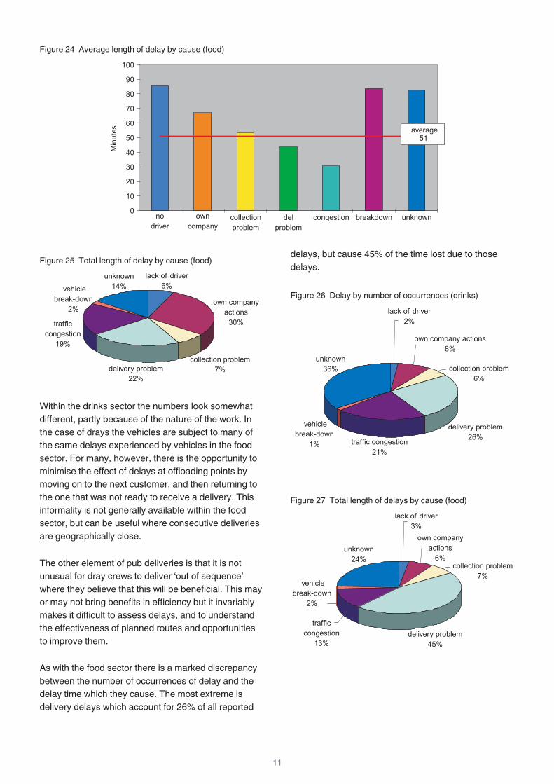
Within the drinks sector the numbers look somewhat

different, partly because of the nature of the work. In

the case of drays the vehicles are subject to many of

the same delays experienced by vehicles in the food

sector. For many, however, there is the opportunity to

minimise the effect of delays at offloading points by

moving on to the next customer, and then returning to

the one that was not ready to receive a delivery. This

informality is not generally available within the food

sector, but can be useful where consecutive deliveries

are geographically close.

The other element of pub deliveries is that it is not

unusual for dray crews to deliver ‘out of sequence’

where they believe that this will be beneficial. This may

or may not bring benefits in efficiency but it invariably

makes it difficult to assess delays, and to understand

the effectiveness of planned routes and opportunities

to improve them.

As with the food sector there is a marked discrepancy

between the number of occurrences of delay and the

delay time which they cause. The most extreme is

delivery delays which account for 26% of all reported

delays, but cause 45% of the time lost due to those

delays.

nodriver

unknownbreakdowncongestion0

10

20

30

40

50

60

70

80

90

100

owncompany

collectionproblem

delproblem

Min

utes average

51

Figure 24 Average length of delay by cause (food)

lack of driver6%

own companyactions

30%

collection problem7%delivery problem

22%

trafficcongestion

19%

vehiclebreak-down

2%

unknown14%

Figure 25 Total length of delay by cause (food)

lack of driver2%

own company actions8%

collection problem6%

delivery problem26%

traffic congestion21%

vehiclebreak-down

1%

unknown36%

Figure 26 Delay by number of occurrences (drinks)

lack of driver3%

own companyactions

6%collection problem

7%

delivery problem45%

trafficcongestion

13%

vehiclebreak-down

2%

unknown24%

Figure 27 Total length of delays by cause (food)

11

2.7 Fuel Consumption and EnergyEfficiency

Fuel ConsumptionFuel consumption data was requested for the period

October 2006 – January 2007. It was considered

worthwhile specifying a three month period to allow

sufficient smoothing of company data to give a

representative figure, but also to minimise the effect of

vehicle replacement programmes had a longer period

been requested.

The overall results were:

Although the composition of the sample group and the

type of work and journeys is likely to be different it is

interesting to note that there appears to have been

relatively little improvement in fuel consumption over a

period of 9 years.

Fuel consumption in the drinks sector was poorer than

food in all vehicle categories, except small rigids. This

may be due to the nature of the work, i.e. short

journeys with large number of deliveries in

predominantly urban areas. Alternatively it may be that

it is an area which has not received a great deal of

management attention, perhaps being seen, in a low

mileage operation, as a relatively small area of

expenditure, and one which is difficult to improve.

Within each vehicle type there is a wide range of fuel

consumption levels, especially in the case of the

smaller vehicles. This may effect the range of journey

type undertaken by rigid vehicles, some of which will

be operating largely in urban environments, whereas

the larger vehicles are more likely to be used on trunk

roads and motorways. Perhaps the most extreme

example of this is the small and medium rigids where

the poorest numbers are generated by inner city

delivery vehicles where the refrigeration equipment is

driven off the vehicle engine.

lack ofdriver

0

10

20

30

40

50

60

70

owncompanyactions

collectionproblem

deliveryproblem

trafficcongestion

vehiclebreak-down

Unknown

Min

utes average

34

Figure 28 Average length of delay by cause (drinks)

Table 5 Fuel Consumption by Vehicle Type

(mpg)(food)

1998 2002 2007

Small rigid 11.3 (4.0) 13.1 (4.7)

Medium rigid 10.4 (3.7) 10.2 (3.6) 9.8 (3.5)

Large rigid 10.4 (3.7) 8.8 (3.1) 10.4 (3.7)

Drawbar 8.8 (3.1) 7.2 (2.5)

City Artic 9.0 (3.2) 9.0 (3.2) 8.5 (3.0)

Medium artic 8.8 (3.1) 9.0 (3.2) 9.3 (3.3)

Large artic 8.2 (2.9) 8.2 (2.9) 8.6 (3.0)

(Table 5 shows kms/litre figures in brackets)

Table 6 Fuel Consumption by Vehicle Type

(mpg)(drinks)

Small rigid 15.1 (5.3)

Medium rigid 8.0 (2.8)

Large rigid 8.2 (2.9)

Drawbar 7.4 (2.6)

City/urban artic 7.0 (2.5)

Medium artic

Large artic 8.6 (3.0)

(Table 6 shows kms/litre figures in brackets)

draw-bar

Worst Average Best

0

2

4

6

8

10

12

14

16

18

20

smallrigid

mediumrigid

largerigid

citysemi-trailers

32 tonnesemi's

38–44semi's

mpg

Figure 29 Fuel consumption by vehicle type (food)

12

Corresponding data for drinks is shown below.

Energy EfficiencyIt has always been difficult to make meaningful

comparisons of transport efficiency between different

operations. There are many variables which will effect

any measure used, including:

the nature and geographical range of the work

undertaken

efficiency of load planning - how is time utilised?

the correct specification of vehicles - are they the

right size and type? - it is very easy to fill

vehicles which are smaller than they should be

the fuel consumption achieved by those

vehicles.

All of these factors effect efficiency, i.e. the amount of

fuel used in moving one unit of load from origin to

destination.

In the last survey a composite measure - pallet kms

per litre - was derived in order to bring some of the

variables together. This has been repeated in the

current Survey and the results are shown below in

Figure 31.

The chart shows clearly that primary operations tend to

be most efficient, with the tertiary the least efficient.

There are some operations which disrupt the pattern

but broadly the results are consistent. They are also as

we might expect, with the typical primary journey –

large vehicle, full load – being the most efficient in

terms of fuel used for product moved.

The numbers clearly show the benefit of moving

product in bulk as far down the supply chain as

possible, before breaking it down into smaller vehicles

and smaller deliveries. The difficulty arises in trying to

do this when most food supply chains have become

increasingly centralised.

As thoughts turn to the environmental impact of the

way that food supply chains are constructed, further

measures will become important. There is an ongoing

drawbar

mediumrigid

largerigid

Worst Average Best

0.00

2.00

4.00

6.00

8.00

10.00

12.00

14.00

16.00

18.00

20.00

smallrigid

city semitrailers

32 44tonnesemi's

�

mpg

Figure 30 Fuel consumption by vehicle type (drinks)

0

10

20

30

40

50

60

70

80

90

100

110

120

130

primary

secondary

tertiary

Fleets

Figure 31 Energy intensity, pallet kms/litre

13

debate about food miles, generally taken to mean the

distance that food travels before it reaches the shelf in

the shop or supermarket. This type of survey cannot

readily identify food miles since it does not follow food

throughout its entire supply chain. We do however

have measures of the number of miles run in moving a

quantity of goods within the supply chain.

Figure 32 shows the average figures for each fleet by

activity, with tertiary operations, generating the most

mileage per pallet moved.

2.8 Operating Restrictions

The Survey also covered, for the first time, the extent to

which fleet operations were affected by local authority

restrictions or by restrictions placed by customers.

Although this area was thought to be of interest many

fleets were unable to respond with sound data.

Only 4.5% of fleets reported local restrictions on the

operation of their own depot, with just two saying that

the restrictions affected both loading/unloading and

vehicle movements.

Delivery restrictions have greater impact with 40% of

food fleets and 59% of drinks fleets reporting customer

delivery time restrictions. The impact was most severe

in food with some fleets reporting that all customers

placed delivery restrictions on them. The extent of the

restrictions is shown in Figure 33 below.

0.0

10.0

20.0

30.0

40.0

50.0

60.0

primary

secondary

tertiary

Fleets

Figure 32 Distance travelled - kms/loaded pallet

0%

10%

20%

30%

40%

50%

60%

70%

80%

90%

100%

Fleets

Figure 33 % of customers with delivery restrictions (food)

0%

10%

20%

30%

40%

50%

60%

Fleets

Figure 34 % of customers with delivery restrictions (drinks)

14

3 Conclusions

3.1 Levels of Efficiency

The 2007 Survey suggests that fuel consumption of

vehicles within the food sector has not improved

drastically since the first survey in 1998. Within the

three groups of rigid vehicles one has improved, one

has worsened and one has remained the same.

Articulated vehicles have shown the best improvement

with all but city artics becoming more fuel efficient over

the 9 year period. Consumption has improved by 6%

and 5% for the two heavier groups.

The reasons for these levels of change cannot be

readily identified from the Survey. There will have been

many changes in the nature of the food supply chains

since 1998, and the mix of the fleets in the last three

Surveys has changed. Nevertheless it is disappointing

that the undoubted improvement in vehicle fuel

efficiency produced by technical advances has not fed

through to operational results. The alternative view is

that, but for those technical and engineering changes,

the changes in the nature of the food supply chain

would have made the fuel consumption figures

significantly worse.

The amount of product carried, or vehicle fill, is one of

the most important measures of utilisation and hence

efficiency. In most cases vehicles carrying food will

reach their volume capacity the weight carrying

capacity. Most food product is not particularly dense

and the increased use of packaging reduces the

density of cases and pallets still further.

Since 2002 the use of height within vehicles has

changed. There are now fewer trips with less than

0.8m of the vehicle’s height used, 5% compared with

9%, and 35 % of trips had product over 1.7m

compared with 15%. Utilisation of vehicle deck space

increased from an average of 69% to an average of

74.8%. Weight utilisation has increased slightly from

53% to 55.1%.

Empty running is a measure of vehicle inefficiency and

most companies will try to eliminate it, since, by

definition, vehicles cannot be earning revenue when

running empty. In practice the level of empty running

will often depend on the type of operation being

considered, but also within operations, on the way in

which vehicle routes are planned. Multi-drop loads

tend to have the lowest empty running since only the

last leg is empty. That last leg can, however, be a long

one if deliveries are made on the outward journey, with

the last drop at the furthest point.

In 2007 the levels of empty running averaged around

24% for the food fleets and 20% for the drinks fleets,

with extremes ranging from virtually none to just less

than 50%.

Time utilisation appears not to have changed

significantly with approximately one third of vehicle

time spent idle and one third spent on the road. The

2007 Survey asked about tractor unit utilisation and as

expected these were much better with almost 50% of

the time spent on the road. The drinks sector faired

worse here with only 22% of time spent on the road

(29% for tractor units).

15

Taken across the day it is clear that primary

movements have become largely a 24 hour operation.

Secondary operations are now spread across 24 hours

with a clear peak during the period which might be

regarded as a normal working day. Tertiary operations

are substantially a ‘day’ operation.

The results for Deviations from Schedule (Delays)

show that traffic congestion is the major reason for

delays to occur, but with a small increase from 31% in

2002 to 32%. The proportion of time lost due to traffic

congestion is, however, much lower at 19%. In the

drinks sector congestion causes 21% of delays but

13% of time lost. The major cause of time lost through

delays, in both food and drinks, is own company

actions and delays at loading and unloading points.

3.2 Utilisation over 24 hours and 7days

The results suggest that, for many operations, vehicles

spend a considerable proportion of their time off the

road, whether pre-loaded or simply idle. The Time

Utilisation charts also show that many operations are

still based around a ‘normal working day’.

Two major problems need to be overcome if this

‘available’ time is to be used. The first is that in most

cases transport operators are aware of the opportunity

but are constrained by the effects of customer delivery

requirements. The second is the likelihood that more

out of hours operations are likely to lead to more

objections from the public, usually because they live

near to transport or warehousing sites, or the premises

receiving deliveries or on the roads leading to them.

These are often seemingly intractable problems, but,

given the size of opportunity they represent they

cannot be allowed to stop all progress in this area.

3.3 Summary

In summary the results show:

Opportunities exist for improvement in vehicle

utilisation but the combination of the 75%

already being achieved and the limitations

imposed by customer service requirements will

probably make further progress increasingly

difficult.

Empty running appears to have increased

Time utilisation remains an issue with vehicles

running on the road for just one third of their

available time.

In food tertiary and drink supply chains most of

the activity takes place during the day, offering

more opportunity for out of hours deliveries. This

is much less the case in secondary operations.

Primary activities are well spread across the

whole 24 hours.

16

Vehicles operations still experience delays but

those with the biggest impact are generated

within suppliers or customers premises rather

than by traffic congestion.

There have been changes in the levels of fuel

consumption achieved but little improvement

overall.

With the advent of seven day trading transport

activities have also become more evenly

distributed across the week. Saturday and

Sunday activities now equate to approximately

1.5 week days, representing a substantial shift of

traffic away from Monday to Friday.

17

Glossary of Terms

This short glossary is included to clarify the definitions of those terms used in the report whose meaning may be open

to interpretation.

Drink Sector

The sector moving alcoholic drinks from manufacturer

or importer to the end user, via retailers, licensed or

off-license premises. Soft drinks would be regarded as

falling into the food sector although relatively small

quantities will have been present on drinks deliveries to

pubs, clubs and restaurants.

Primary

Movement of saleable product, raw material, work in

progress, returns, packaging or handling equipment

between a supplier and factory/factory and NDC/NDC

and customer’s RDC, Hub depot or Wholesale depot

including ‘Cash & Carry’s.

Secondary

Movement of saleable product from retailer RDC or

Food Service Hub depot into retail outlet or picking

depot. In addition, the return of equipment or goods

from outlet to RDC or Hub.

Tertiary

Movement of saleable goods from a factory, regional

or picking depot, including wholesaler, into the final

outlet where product is consumed i.e. home, pubs &

clubs, small independent corner shops, retail

forecourts or restaurants.

Urban Artic

A tractor and semi trailer combination which has been

specified to operate specifically in an urban

environment where access and manoeuvring space

might be limited. The tractor will invariably have a

single rear axle and usually have a gross combination

weight of no more than around 26 tonnes. The semi-

trailer will usually be single axle and probably 7-10

metres long.

Drawbar

A vehicle consisting of a combination of a rigid vehicle

towing a trailer, that is a trailer which supports its own

weight independently rather than imposing some of it

on the drawing vehicle.

18

FreightBestPractice

Key Performance Indicators forFood and Drink Supply Chains

November 2007.

Printed in the UK on paper containing at least 75% recycled fibre.

FBP1086 # Queens Printer and Controller of HMSO 2007.

BenchmarkingGuide