Karush-Kuhn-Tucker Conditions · rf(x) = 0 That is, f(x) ... Inequality Constrained Optimization (jg These conditions are known as the Karush-Kuhn-Tucker Conditions

Karush-Kuhn-Tucker Conditions

Richard Lusby

Department of Management EngineeringTechnical University of Denmark

Today’s Topics(jg

Unconstrained Optimization

Equality Constrained Optimization

Equality/Inequality Constrained Optimization

R Lusby (42111) KKT Conditions 2/40

Unconstrained Optimization


Unconstrained Optimization(jg

Problem

minimize f (x)

subject to: x ∈ Rn

First Order Necessary Conditions

If x∗ is a local minimizer of f (x) and f (x) is continuously differentiable inan open neighbourhood of x∗, then

∇f (x∗) = 0

That is, f (x) is stationary at x∗


Unconstrained Optimization(jg

Second Order Necessary Conditions

If x∗ is a local minimizer of f (x) and ∇2f (x) is continuously differentiablein an open neighbourhood of x∗, then

∇f (x∗) = 0

∇2f (x∗) is positive semi definite

Second Order Sufficient Conditions

Suppose that ∇2f (x) is continuously differentiable in an openneighbourhood of x∗. If the following two conditions are satisfied, then x∗

is a local minimum of f (x).

∇f (x∗) = 0

∇2f (x∗) is positive definite


Equality Constrained Optimization


Equality Constrained Optimization(jg

Problem

minimize f (x)

subject to: hi (x) = 0 ∀i = 1, 2, . . .m

x ∈ Rn


Equality Constrained OptimizationConsider the following example(jg

Example

minimize 2x21 + x22subject to: x1 + x2 = 1

Let us first consider the unconstrained case

Differentiate with respect to x1 and x2

∂f (x1, x2)

∂x1= 4x1

∂f (x1, x2)

∂x2= 2x2

These yield the solution x1 = x2 = 0

Does not satisfy the constraint


Equality Constrained OptimizationExample Continued(jg

Let us penalize ourselves for not satisfying the constraint

This gives

L(x1, x2, λ1) = 2x21 + x22 + λ1(1− x1 − x2)

This is known as the Lagrangian of the problem

Try to adjust the value λ1 so we use just the right amount of resource

λ1 = 0→ get solution x1 = x2 = 0, 1− x1 − x2 = 1

λ1 = 1→ get solution x1 = 14 , x2 = 1

2 , 1− x1 − x2 = 14

λ1 = 2→ get solution x1 = 12 , x2 = 1, 1− x1 − x2 = −1

2

λ1 = 43 → get solution x1 = 1

3 , x2 = 23 , 1− x1 − x2 = 0


Equality Constrained OptimizationGenerally Speaking(jg

Given the following Non-Linear Program

Problem

minimize f (x)

subject to: hi (x) = 0 ∀i = 1, 2, . . .m

x ∈ Rn

A solution can be found using the Lagrangian

L(x,λ) = f (x) +m∑i=1

λi (0− hi (x))


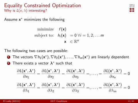
Equality Constrained OptimizationWhy is L(x , λ) interesting?(jg

Assume x∗ minimizes the following

minimize f (x)

subject to: hi (x) = 0 ∀i = 1, 2, . . .m

x ∈ Rn

The following two cases are possible:

1 The vectors ∇h1(x∗),∇h2(x∗), . . . ,∇hm(x∗) are linearly dependent

2 There exists a vector λ∗ such that

∂L(x∗,λ∗)∂x1

=∂L(x∗,λ∗)

∂x2=∂L(x∗,λ∗)

∂x3=, . . . ,=

∂L(x∗,λ∗)∂xn

= 0

∂L(x∗,λ∗)∂λ1

=∂L(x∗,λ∗)

∂λ2=∂L(x∗,λ∗)

∂λ3=, . . . ,=

∂L(x∗,λ∗)∂λm

= 0


Case 1: Example(jg

Example

minimize x1 + x2 + x23subject to: x1 = 1

x21 + x22 = 1

The minimum is achieved at x1 = 1, x2 = 0, x3 = 0

The Lagrangian is:

L(x1, x2, x3, λ1, λ2) = x1 + x2 + x23 + λ1(1− x1) + λ2(1− x21 − x22 )

Observe that:∂L(1, 0, 0, λ1, λ2)

∂x2= 1 ∀λ1, λ2

Observe ∇h1(1, 0, 0) =[

1 0 0]

and ∇h2(1, 0, 0) =[

2 0 0]


Case 2: Example(jg

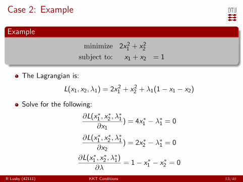
Example

minimize 2x21 + x22subject to: x1 + x2 = 1

The Lagrangian is:

L(x1, x2, λ1) = 2x21 + x22 + λ1(1− x1 − x2)

Solve for the following:

∂L(x∗1 , x∗2 , λ

∗1

∂x1) = 4x∗1 − λ∗1 = 0

∂L(x∗1 , x∗2 , λ

∗1

∂x2) = 2x∗2 − λ∗1 = 0

∂L(x∗1 , x∗2 , λ

∗1)

∂λ= 1− x∗1 − x∗2 = 0


Case 2: Example continued(jg

Solving this system of equations yields x∗1 = 13 , x∗2 = 2

3 , λ∗1 = 4

3

Is this a minimum or a maximum?


Graphically(jg

x1

x2

x1 + x2 = 1

1

1


Graphically(jg

x1

x2

x1 + x2 = 1

1

1x∗1 = 13

x∗2 = 23

∇f (x∗) = λ∗∇h(x∗)


Geometric Interpretation(jg

Consider the gradients of f and h at the optimal point

They must point in the same direction, though they may havedifferent lengths

∇f (x∗) = λ∗∇h(x∗)

Along with feasibility of x∗, is the condition ∇L(x∗,λ∗) = 0

From the example, at x∗1 = 13 , x∗2 = 2

3 , λ∗1 = 4

3

∇f (x∗1 , x∗2 ) =

[4x∗1 2x∗2

]=

[43

43

]∇h1(x∗1 , x

∗2 ) =

[1 1

]


Geometric Interpretation(jg

∇f (x) points in the direction of steepest ascent

−∇f (x) points in the direction of steepest descent

In two dimensions:I ∇f (xo) is perpendicular to a level curve of f

I ∇hi (xo) is perpendicular to the level curve hi (xo) = 0


Equality, Inequality Constrained Optimization


Inequality ConstraintsWhat happens if we now include inequality constraints?(jg

General Problem

maximize f (x)

subject to: gi (x) ≤ 0 (µi ) ∀i ∈ I

hj(x) = 0 (λj) ∀i ∈ J

Given a feasible solution xo, the set of binding constraints is:

I = {i : gi (xo) = 0}


The Lagrangian(jg

L(x,λ,µ) = f (x) +m∑i=1

µi (0− gi (x)) +k∑

j=1

λj(0− hj(x))


Inequality Constrained Optimization(jg

Assume x∗ maximizes the following

maximize f (x)

subject to: gi (x) ≤ 0 (µi ) ∀i ∈ I

hj(x) = 0 (λj) ∀i ∈ J

The following two cases are possible:

1 ∇h1(x∗), . . . ,∇hk(x∗),∇g1(x∗), . . . ,∇gm(x∗) are linearly dependent

2 There exist vectors λ∗ and µ∗ such that

∇f (x∗)−k∑

j=1

λj∇hj(x∗)−m∑i=1

µi∇gi (x∗) = 0

µ∗i gi (x∗) = 0

µ∗ ≥ 0


Inequality Constrained Optimization(jg

These conditions are known as the Karush-Kuhn-Tucker Conditions

We look for candidate solutions x∗ for which we can find λ∗ and µ∗

Solve these equations using complementary slackness

At optimality some constraints will be binding and some will be slack

Slack constraints will have a corresponding µi of zero

Binding constraints can be treated using the Lagrangian


Constraint qualifications(jg

KKT constraint qualification

∇gi (xo) for i ∈ I are linearly independent

Slater constraint qualification

gi (x) for i ∈ I are convex functionsA non boundary point exists: gi (x) < 0 for i ∈ I


Case 1 Example(jg

The Problem

maximize x

subject to: y ≤ (1− x)3

y ≥ 0

Consider the global max: (x , y) = (1, 0)

After reformulation, the gradients are

∇f (x , y) = (1, 0)

∇g1 = (3(x − 1)2, 1)

∇g2 = (0,−1)

Consider ∇f (x , y)−∑2

i=1 µi∇gi (x , y)


Graphically(jg

x

y

y = (1− x)3

1

1


Case 1 Example(jg

We get: [1

0

]− µ1

[0

1

]− µ2

[0

−1

]

No µ1 and µ2 exist such that:

∇f (x , y)−2∑

i=1

µi∇gi (x , y) = 0


Case 2 Example(jg

The Problem

maximize −(x − 2)2 − 2(y − 1)2

subject to: x + 4y ≤ 3

x ≥ y

The Problem (Rearranged)

maximize −(x − 2)2 − 2(y − 1)2

subject to: x + 4y ≤ 3

−x + y ≤ 0


Case 2 Example(jg

The Lagrangian is:

L(x1, y , µ1, µ2) = −(x−2)2−2(y−1)2+µ1(3−x−4y)+µ2(0+x−y)

This gives the following KKT conditions

∂L

∂x= −2(x − 2)− µ1 + µ2 = 0

∂L

∂y= −4(y − 1)− 4µ1 − µ2 = 0

µ1(3− x − 4y) = 0

µ2(x − y) = 0

µ1, µ2 ≥ 0


Case 2 ExampleContinued(jg

We have two complementarity conditions → check 4 cases

1 µ1 = µ2 = 0→ x = 2, y = 1

2 µ1 = 0, x − y = 0→ x = 43 , µ2 = −4

3

3 3− x − 4y = 0, µ2 = 0→ x = 53 , y = 1

3 , µ1 = 23

4 3− x − 4y = 0, x − y = 0→ x = 35 , y = 3

5 , µ1 = 2225 , µ2 = −48

25

Optimal solution is therefore x∗ = 53 , y∗ = 1

3 , f (x∗, y∗) = −49


Case 2 ExampleContinued(jg

We have two complementarity conditions → check 4 cases

1 µ1 = µ2 = 0→ x = 2, y = 1

2 µ1 = 0, x − y = 0→ x = 43 , µ2 = −4

3

3 3− x − 4y = 0, µ2 = 0→ x = 53 , y = 1

3 , µ1 = 23

4 3− x − 4y = 0, x − y = 0→ x = 35 , y = 3

5 , µ1 = 2225 , µ2 = −48

25

Optimal solution is therefore x∗ = 53 , y∗ = 1

3 , f (x∗, y∗) = −49


Continued(jg

The Problem

minimize (x − 3)2 + (y − 2)2

subject to: x2 + y2 ≤ 5

x + 2y ≤ 4

x , y ≥ 0

The Problem (Rearranged)

maximize −(x − 3)2 − (y − 2)2


x + 2y ≤ 4

−x ,−y ≤ 0


Inequality Example(jg

The gradients are:

∇f (x , y) = (6− 2x , 4− 2y)

∇g1(x , y) = (2x , 2y)

∇g2(x , y) = (1, 2)

∇g3(x , y) = (−1, 0)

∇g4(x , y) = (0,−1)


Inequality ExampleContinued(jg

Consider the point (x , y) = (2, 1)

It is feasible I = {1, 2}

This gives [2

2

]− µ1

[4

2

]− µ2

[1

2

]=

[0

0

]

µ1 = 13 , µ2 = 2

3 satisfy this


Sufficient condition(jg

General Problem

maximize f (x)

subject to: gi (x) ≤ 0 ∀i ∈ I

Theorem

If f (x) is concave and gi (x) for i ∈ I are convex functions then a feasibleKKT point is optimal

An equality constraint is equivalent to two inequality constraints:

hj(x) = 0⇔ hj(x) ≤ 0 and − hj(x) ≤ 0

The corresponding two nonnegative multipliers may be combined toone free one

λj+∇h(x) + λj−(−∇h(x)) = λj∇h(x)


Equality constraints(jg

General Problem

maximize f (x)


hj(x) = 0 ∀j ∈ J

Let xo be a feasible solution

As before, I = {i : gi (xo) = 0}

Assume constraint qualification holds


Equality constraintsContinued(jg

KKT Necessary Optimality Conditions

If xo is a local maximum, there exist multipliers µi ≥ 0 ∀i ∈ I and λj∀j ∈ J such that

∇f (xo)−∑i∈I

µi∇gi (xo)−∑j

λj∇hj(xo) = 0

KKT Sufficient Optimality Conditions

If f (x) is concave, gi (x) ∀ i ∈ I are convex functions and hj ∀j ∈ J areaffine (linear) then a feasible KKT point is optimal


KKT Conditions - Summary(jg

General Problem

maximize f (x)


hj(x) = 0 ∀j ∈ J

KKT conditions

∇f (xo)−∑

i µi∇gi (xo)−∑

j λj∇hj(xo) = 0

µigi (xo) = 0 ∀i ∈ I

µi ≥ 0 ∀i ∈ I

xo feasible


Alternative FormulationVector Function Form(jg

General Problem

maximize f (x)

subject to: g(x) ≤ 0

h(x) = 0

KKT Conditions

∇f (xo)− µ∇g(xo)− λ∇h(xo) = 0

µg(xo) = 0

µ ≥ 0

xo feasible


Class Exercise 1(jg

The Problem

maximize ln(x + 1) + y

subject to: 2x + y ≤ 3

x , y ≥ 0


Class Exercise 2(jg

The problem

minimize x2 + y2


x + 2y = 4

x , y ≥ 0


Class Exercise 3(jg

Write the KKT conditions for

maximize cTx

subject to: Ax ≤ b

x ≥ 0


Documents

Karush-Kuhn-Tucker Conditions · rf(x) = 0 That is, f(x) ... Inequality Constrained Optimization (jg These conditions are known as the Karush-Kuhn-Tucker Conditions