Report no. 07/18

Kalman Filtering with Equality and Inequality StateConstraints

Nachi Gupta Raphael HauserOxford University Computing Laboratory, Numerical Analysis Group,

Wolfson Building, Parks Road, Oxford OX1 3QD, U.K.

Both constrained and unconstrained optimization problems regularly appearin recursive tracking problems engineers currently address – however, constraintsare rarely exploited for these applications. We define the Kalman Filter anddiscuss two different approaches to incorporating constraints. Each of theseapproaches are first applied to equality constraints and then extended to inequalityconstraints. We discuss methods for dealing with nonlinear constraints and forconstraining the state prediction. Finally, some experiments are provided toindicate the usefulness of such methods.

Key words and phrases: Constrained optimization, Kalman filtering, Nonlinear filters,Optimization methods, Quadratic programming, State estimation

Oxford University Computing LaboratoryNumerical Analysis GroupWolfson BuildingParks RoadOxford, England OX1 3QDE-mail: nachi@comlab.oxford.ac.uk August, 2007

2

1 IntroductionKalman Filtering [8] is a method to make real-time predictions for systems with someknown dynamics. Traditionally, problems requiring Kalman Filtering have been complexand nonlinear. Many advances have been made in the direction of dealing with nonlinearities(e.g., Extended Kalman Filter [1], Unscented Kalman Filter [7]). These problems also tend tohave inherent state space equality constraints (e.g., a fixed speed for a robotic arm) and statespace inequality constraints (e.g., maximum attainable speed of a motor). In the past, lessinterest has been generated towards constrained Kalman Filtering, partly because constraintscan be difficult to model. As a result, constraints are often neglected in standard KalmanFiltering applications.

The extension to Kalman Filtering with known equality constraints on the state space isdiscussed in [5, 12–14, 16]. In this paper, we discuss two distinct methods to incorporateconstraints into a Kalman Filter. Initially, we discuss these in the framework of equalityconstraints. The first method, projecting the updated state estimate onto the constrainedregion, appears with some discussion in [5, 12]. We propose another method, which is torestrict the optimal Kalman Gain so the updated state estimate will not violate the constraint.With some algebraic manipulation, the second method is shown to be a special case of thefirst method.

We extend both of these concepts to Kalman Filtering with inequality constraints in thestate space. This generalization for the first approach was discussed in [11].1 Constrainingthe optimal Kalman Gain was briefly discussed in [10]. Further, we will also make theextension to incorporating state space constraints in Kalman Filter predictions.

Analogous to the way a Kalman Filter can be extended to solve problems containingnon-linearities in the dynamics using an Extended Kalman Filter by linearizing locally (orby using an Unscented Kalman Filter), linear inequality constrained filtering can similarly beextended to problems with nonlinear constraints by linearizing locally (or by way of anotherscheme like an Unscented Kalman Filter). The accuracy achieved by methods dealing withnonlinear constraints will naturally depend on the structure and curvature of the nonlinearfunction itself. In the two experiments we provide, we look at incorporating inequalityconstraints to a tracking problem with nonlinear dynamics.

2 Kalman FilterA discrete-time Kalman Filter [8] attempts to find the best running estimate for a recursivesystem governed by the following model2:

xk = Fk,k−1xk−1 + uk,k−1, uk,k−1 ∼ N (0, Qk,k−1) (2.1)

1The similar extension for the method of [16] was made in [6].2The subscript k on a variable stands for the k-th time step, the mathematical notation N (µ,Σ) denotes a

normally distributed random vector with mean µ and covariance Σ, and all vectors in this paper are columnvectors (unless we are explicitly taking the transpose of the vector).

3

zk = Hkxk + vk, vk ∼ N (0, Rk) (2.2)

Here xk is an n-vector that represents the true state of the underlying system and Fk,k−1

is an n × n matrix that describes the transition dynamics of the system from xk−1 to xk.The measurement made by the observer is an m-vector zk, and Hk is an m × n matrix thattransforms a vector from the state space into the appropriate vector in the measurement space.The noise terms uk,k−1 (an n-vector) and vk (an m-vector) encompass known and unknownerrors in Fk,k−1 and Hk and are normally distributed with mean 0 and covariances givenby n × n matrix Qk,k−1 and m × m matrix Rk, respectively. At each iteration, the KalmanFilter makes a state prediction for xk, denoted xk|k−1. We use the notation k|k − 1 since wewill only use measurements provided until time-step k−1 in order to make the prediction attime-step k. The state prediction error xk|k−1 is defined as the difference between the truestate and the state prediction, as below.

xk|k−1 = xk − xk|k−1 (2.3)

The covariance structure for the expected error on the state prediction is defined asthe expectation of the outer product of the state prediction error. We call this covariancestructure the error covariance prediction and denote it Pk|k−1.3

Pk|k−1 = E[(

xk|k−1

) (xk|k−1

)′] (2.4)

The filter will also provide an updated state estimate for xk, given all the measurementsprovided up to and including time step k. We denote these estimates by xk|k. We similarlydefine the state estimate error xk|k as below.

xk|k = xk − xk|k (2.5)

The expectation of the outer product of the state estimate error represents the covariancestructure of the expected errors on the state estimate, which we call the updated errorcovariance and denote Pk|k.

Pk|k = E[(

xk|k) (

xk|k)′] (2.6)

At time-step k, we can make a prediction for the underlying state of the system byallowing the state to transition forward using our model for the dynamics and noting thatE [uk,k−1] = 0. This serves as our state prediction.

xk|k−1 = Fk,k−1xk−1|k−1 (2.7)

If we expand the expectation in Equation (2.4), we have the following equation for theerror covariance prediction.

Pk|k−1 = Fk,k−1Pk−1|k−1F′k,k−1 + Qk,k−1 (2.8)

3We use the prime notation on a vector or a matrix to denote its transpose throughout this paper.

4

We can transform our state prediction into the measurement space, which is a predictionfor the measurement we now expect to observe.

zk|k−1 = Hkxk|k−1 (2.9)

The difference between the observed measurement and our predicted measurement is themeasurement residual, which we are hoping to minimize in this algorithm.

νk = zk − zk|k−1 (2.10)

We can also calculate the associated covariance for the measurement residual, which isthe expectation of the outer product of the measurement residual with itself, E [νkν

′k]. We

call this the measurement residual covariance.

Sk = HkPk|k−1H′k + Rk (2.11)

We can now define our updated state estimate as our prediction plus some perturbation,which is given by a weighting factor times the measurement residual. The weighting factor,called the Kalman Gain, will be discussed below.

xk|k = xk|k−1 + Kkνk (2.12)

Naturally, we can also calculate the updated error covariance by expanding the outerproduct in Equation (2.6).4

Pk|k = (I−KkHk) Pk|k−1 (I−KkHk)′ + KkRkK

′k (2.13)

Now we would like to find the Kalman Gain Kk, which minimizes the mean square stateestimate error, E

[∣∣xk|k∣∣2]. This is the same as minimizing the trace of the updated error

covariance matrix above.5 After some calculus, we find the optimal gain that achieves this,written below.6

Kk = Pk|k−1H′kS

−1k (2.14)

The covariance matrices in the Kalman Filter provide us with a measure for uncertaintyin our predictions and updated state estimate. This is a very important feature for the variousapplications of filtering since we then know how much to trust our predictions and estimates.Also, since the method is recursive, we need to provide an initial covariance that is largeenough to contain the initial state to ensure comprehensible performance. For a more detaileddiscussion of Kalman Filtering, we refer the reader to the following book [1].

4The I in Equation (2.13) represents the n × n identity matrix. Throughout this paper, we use I to denotethe same matrix, except in Appendix A, where I is the appropriately sized identity matrix.

5Note that v′v = trace [vv′] for some vector v.6We could also minimize the mean square state estimate error in the N norm, where N is a positive definite

and symmetric weighting matrix. In the N norm, the optimal gain would be KNk = N

12 Kk.

5

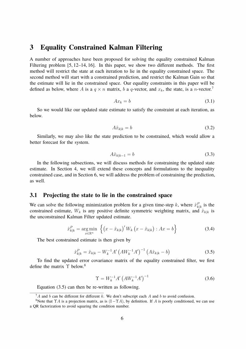
3 Equality Constrained Kalman FilteringA number of approaches have been proposed for solving the equality constrained KalmanFiltering problem [5, 12–14, 16]. In this paper, we show two different methods. The firstmethod will restrict the state at each iteration to lie in the equality constrained space. Thesecond method will start with a constrained prediction, and restrict the Kalman Gain so thatthe estimate will lie in the constrained space. Our equality constraints in this paper will bedefined as below, where A is a q × n matrix, b a q-vector, and xk, the state, is a n-vector.7

Axk = b (3.1)

So we would like our updated state estimate to satisfy the constraint at each iteration, asbelow.

Axk|k = b (3.2)

Similarly, we may also like the state prediction to be constrained, which would allow abetter forecast for the system.

Axk|k−1 = b (3.3)

In the following subsections, we will discuss methods for constraining the updated stateestimate. In Section 4, we will extend these concepts and formulations to the inequalityconstrained case, and in Section 6, we will address the problem of constraining the prediction,as well.

3.1 Projecting the state to lie in the constrained spaceWe can solve the following minimization problem for a given time-step k, where xP

k|k is theconstrained estimate, Wk is any positive definite symmetric weighting matrix, and xk|k isthe unconstrained Kalman Filter updated estimate.

xPk|k = arg min

x∈Rn

{(x − xk|k

)′Wk

(x − xk|k

): Ax = b

}(3.4)

The best constrained estimate is then given by

xPk|k = xk|k − W−1

k A′ (AW−1k A′)−1 (

Axk|k − b)

(3.5)

To find the updated error covariance matrix of the equality constrained filter, we firstdefine the matrix Υ below.8

Υ = W−1k A′ (AW−1

k A′)−1 (3.6)

Equation (3.5) can then be re-written as following.7A and b can be different for different k. We don’t subscript each A and b to avoid confusion.8Note that ΥA is a projection matrix, as is (I−ΥA), by definition. If A is poorly conditioned, we can use

a QR factorization to avoid squaring the condition number.

6

xPk|k = xk|k − Υ

(Axk|k − b

)(3.7)

We can find a reduced form for xk − xPk|k as below.

xk − xPk|k = xk − xk|k + Υ

(Axk|k − b − (Axk − b)

)(3.8a)

= xk − xk|k + Υ(Axk|k − Axk

)(3.8b)

= − (I−ΥA)(xk|k − xk

)(3.8c)

Using the definition of the error covariance matrix, we arrive at the following expression.

P Pk|k = E

[(xk − xP

k|k) (

xk − xPk|k

)′] (3.9a)

= E[(I−ΥA)

(xk|k − xk

) (xk|k − xk

)′(I−ΥA)′

](3.9b)

= (I−ΥA) Pk|k (I−ΥA)′ (3.9c)= Pk|k − ΥAPk|k − Pk|kA

′Υ′ + ΥAPk|kA′Υ′ (3.9d)

= Pk|k − ΥAPk|k (3.9e)= (I−ΥA) Pk|k (3.9f)

It can be shown that choosing Wk = P−1k|k results in the smallest updated error covariance.

This also provides a measure of the information in the state at k.9

3.2 Restricting the optimal Kalman Gain so the updated state estimatelies in the constrained space

Alternatively, we can expand the updated state estimate term in Equation (3.2) using Equation(2.12).

A(xk|k−1 + Kkνk

)= b (3.10)

Then, we can choose a Kalman Gain KRk , that forces the updated state estimate to be in

the constrained space. In the unconstrained case, we chose the optimal Kalman Gain Kk,by solving the minimization problem below which yields Equation (2.14).

Kk = arg minK∈Rn×m

trace[(I−KHk) Pk|k−1 (I−KHk)

′ + KRkK′] (3.11)

Now we seek the optimal KRk that satisfies the constrained optimization problem written

below for a given time-step k.9If M and N are covariance matrices, we say N is smaller than M if M − N is positive semidefinite.

Another formulation for incorporating equality constraints into a Kalman Filter is by observing the constraintsas pseudo-measurements [14, 16]. When Wk is chosen to be P−1

k|k , both of these methods are mathematicallyequivalent [5]. Also, a more numerically stable form of Equation (3.9) with discussion is provided in [5].

7

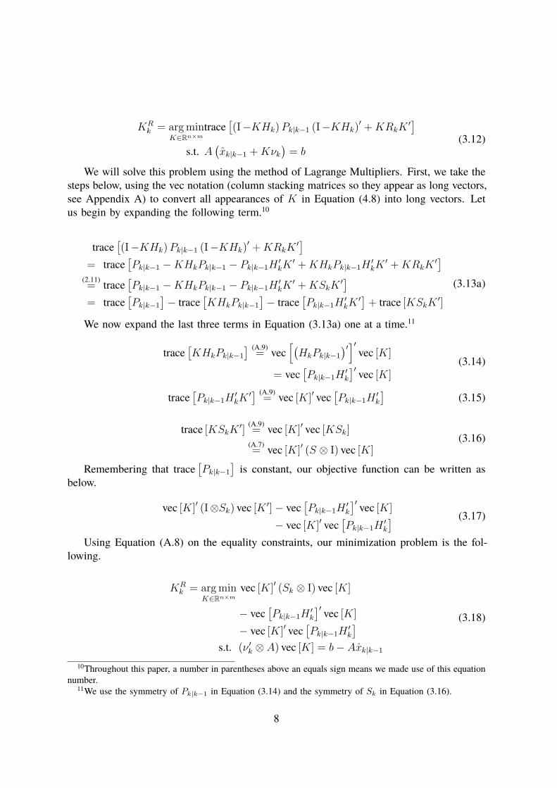
KRk = arg min

K∈Rn×m

trace[(I−KHk) Pk|k−1 (I−KHk)

′ + KRkK′]

s.t. A(xk|k−1 + Kνk

)= b

(3.12)

We will solve this problem using the method of Lagrange Multipliers. First, we take thesteps below, using the vec notation (column stacking matrices so they appear as long vectors,see Appendix A) to convert all appearances of K in Equation (4.8) into long vectors. Letus begin by expanding the following term.10

trace[(I−KHk) Pk|k−1 (I−KHk)

′ + KRkK′]

= trace[Pk|k−1 − KHkPk|k−1 − Pk|k−1H

′kK

′ + KHkPk|k−1H′kK

′ + KRkK′]

(2.11)= trace

[Pk|k−1 − KHkPk|k−1 − Pk|k−1H

′kK

′ + KSkK′]

= trace[Pk|k−1

]− trace

[KHkPk|k−1

]− trace

[Pk|k−1H

′kK

′] + trace [KSkK′]

(3.13a)

We now expand the last three terms in Equation (3.13a) one at a time.11

trace[KHkPk|k−1

] (A.9)= vec

[(HkPk|k−1

)′]′ vec [K]

= vec[Pk|k−1H

′k

]′ vec [K](3.14)

trace[Pk|k−1H

′kK

′] (A.9)= vec [K]′ vec

[Pk|k−1H

′k

](3.15)

trace [KSkK′]

(A.9)= vec [K]′ vec [KSk]

(A.7)= vec [K]′ (S ⊗ I) vec [K]

(3.16)

Remembering that trace[Pk|k−1

]is constant, our objective function can be written as

below.

vec [K]′ (I⊗Sk) vec [K ′] − vec[Pk|k−1H

′k

]′ vec [K]

− vec [K]′ vec[Pk|k−1H

′k

] (3.17)

Using Equation (A.8) on the equality constraints, our minimization problem is the fol-lowing.

KRk = arg min

K∈Rn×m

vec [K]′ (Sk ⊗ I) vec [K]

− vec[Pk|k−1H

′k

]′ vec [K]

− vec [K]′ vec[Pk|k−1H

′k

]s.t. (ν ′

k ⊗ A) vec [K] = b − Axk|k−1

(3.18)

10Throughout this paper, a number in parentheses above an equals sign means we made use of this equationnumber.

11We use the symmetry of Pk|k−1 in Equation (3.14) and the symmetry of Sk in Equation (3.16).

8

Further, we simplify this problem so the minimization problem has only one quadraticterm. We complete the square as follows. We want to find the unknown variable µ which willcancel the linear term. Let the quadratic term appear as follows. Note that the non-“vec [K]"term is dropped as is is irrelevant for the minimization problem.

(vec [K] + µ)′ (Sk ⊗ I) (vec [K] + µ) (3.19)

The linear term in the expansion above is the following.

vec [K]′ (Sk ⊗ I) µ + µ′ (Sk ⊗ I) vec [K] (3.20)

So we require that the two equations below hold.

(Sk ⊗ I) µ = −vec[Pk|k−1H

′k

]µ′ (Sk ⊗ I) = −vec

[Pk|k−1H

′k

]′ (3.21)

This leads to the following value for µ.

µ(A.3)= −

(S−1

k ⊗ I)

vec[Pk|k−1H

′k

](A.8)= −vec

[Pk|k−1H

′kS

−1k

](2.14)= −vec [Kk]

(3.22)

Using Equation (A.6), our quadratic term in the minimization problem becomes thefollowing.

(vec [K − Kk])′ (Sk ⊗ I) (vec [K − Kk]) (3.23)

Let l = vec [K − Kk]. Then our minimization problem becomes the following.

KRk = arg min

l∈Rmn

l′ (Sk ⊗ I) l

s.t. (ν ′k ⊗ A) (l + vec [Kk]) = b − Axk|k−1

(3.24)

We can then re-write the constraint taking the vec [Kk] term to the other side as below.

(ν ′k ⊗ A) l = b − Axk|k−1 − (ν ′

k ⊗ A) vec [Kk](A.8)= b − Axk|k−1 − vec [AKkνk]

= b − Axk|k−1 − AKkνk

(2.12)= b − Axk|k

(3.25)

This results in the following simplified form.

KRk = arg min

l∈Rmn

l′ (Sk ⊗ I) l

s.t. (ν ′k ⊗ A) l = b − Axk|k

(3.26)

We form the Lagrangian L, where we introduce q Lagrange Multipliers in vector λ =(λ1, λ2, . . . , λq)

′

9

L =l′ (Sk ⊗ I) l − λ′ [(ν ′k ⊗ A) l − b + Axk|k

](3.27)

We take the partial derivative with respect to l.12

∂L∂l

= 2l′ (Sk ⊗ I) − λ′ (ν ′k ⊗ A) (3.28)

Similarly we can take the partial derivative with respect to the vector λ.

∂L∂λ

= (ν ′k ⊗ A) l − b + Axk|k (3.29)

When both of these derivatives are set equal to the appropriate size zero vector, we havethe solution to the system. Taking the transpose of Equation (3.28), we can write this systemas Mn = p with the following block definitions for M,n, and p.

M =

[2Sk ⊗ I νk ⊗ A′

ν ′k ⊗ A 0[q×q]

](3.30)

n =

[lλ

](3.31)

p =

[0[mn×1]

b − Axk|k

](3.32)

We solve this system for vector n in Appendix C. The solution for l is pasted below.([S−1

k νk

(ν ′

kS−1k νk

)−1]⊗

[A′ (AA′)

−1]) (

b − Axk|k)

(3.33)

Bearing in mind that b−Axk|k = vec[b − Axk|k

], we can use Equation (A.8) to re-write

l as below.13

vec[A′ (AA′)

−1 (b − Axk|k

) (ν ′

kS−1k νk

)−1ν ′

kS−1k

](3.34)

The resulting matrix inside the vec operation is then an n by m matrix. Rememberingthe definition for l, we notice that K − Kk results in an n by m matrix also. Since both ofthe components inside the vec operation result in matrices of the same size, we can safelyremove the vec operation from both sides. This results in the following optimal constrainedKalman Gain KR

k .

Kk − A′ (AA′)−1 (

Axk|k − b) (

ν ′kS

−1k νk

)−1ν ′

kS−1k (3.35)

If we now substitute this Kalman Gain into Equation (2.12) to find the constrainedupdated state estimate, we end up with the following.

xRk|k = xk|k − A′ (AA′)

−1 (Axk|k − b

)(3.36)

12We used the symmetry of (Sk ⊗ I) here.13Here we used the symmetry of S−1

k and(ν′

kS−1k νk

)−1 (the latter of which is actually just a scalar).

10

This is of course equivalent to the result of Equation (3.5) with the weighting matrix Wk

chosen as the identity matrix. The error covariance for this estimate is given by Equation(3.9).14

4 Adding Inequality ConstraintsIn the more general case of this problem, we may encounter equality and inequality con-straints, as given below.15

Axk = b

Cxk ≤ d(4.1)

So we would like our updated state estimate to satisfy the constraint at each iteration, asbelow.

Axk|k = b

Cxk|k ≤ d(4.2)

Similarly, we may also like the state prediction to be constrained, which would allow abetter forecast for the system.

Axk|k−1 = b

Cxk|k−1 ≤ d(4.3)

We will present two analogous methods to those presented for the equality constrainedcase. In the first method, we will run the unconstrained filter, and at each iteration constrainthe updated state estimate to lie in the constrained space. In the second method, we willfind a Kalman Gain KR

k such that the the updated state estimate will be forced to lie in theconstrained space. In both methods, we will no longer be able to find an analytic solutionas before. Instead, we use numerical methods.

4.1 By Projecting the Unconstrained EstimateGiven the best unconstrained estimate, we could solve the following minimization problemfor a given time-step k, where xP

k|k is the inequality constrained estimate and Wk is anypositive definite symmetric weighting matrix.

14We can use the unconstrained or constrained Kalman Gain to find this error covariance matrix. Since theconstrained Kalman Gain is suboptimal for the unconstrained problem, before projecting onto the constrainedspace, the constrained covariance will be different from the unconstrained covariance. However, the differencelies exactly in the space orthogonal to which the covariance is projected onto by Equation (3.9). The proof isomitted for brevity.

15C and d can be different for different k. We don’t subscript each C and d to simplify notation.

11

xPk|k = arg min

x

(x − xk|k

)′Wk

(x − xk|k

)s.t. Ax = b

Cx ≤ d

(4.4)

For solving this inequality constrained optimization problem, we can use a variety ofstandard methods, or even an out-of-the-box solver, like fmincon in Matlab. Here we usean active set method [4]. This is a common method for dealing with inequality constraints,where we treat a subset of the constraints (called the active set) as additional equalityconstraints. We ignore any inactive constraints when solving our optimization problem.After solving the problem, we check if our solution lies in the space given by the inequalityconstraints. If it doesn’t, we start from the solution in our previous iteration and move in thedirection of the new solution until we hit a set of constraints. For each iteration, the activeset is made up of those inequality constraints with non-zero Lagrange Multipliers.

We first find the best estimate (using Equation (3.5) for the equality constrained problemwith the equality constraints given in Equation (4.1) plus the active set of inequality con-straints. Let us call the solution to this xP∗

k|k,j since we have not yet checked if the solutionlies in the inequality constrained space.16 In order to check this, we find the vector that wemoved along to reach xP∗

k|k,j . This is given by the following.

s = xP∗k|k,j − xP

k|k,j−1 (4.5)

We now iterate through each of our inequality constraints, to check if they are satisfied.If they are all satisfied, we choose τmax = 1. If they are not, we choose the largest valueof τmax such that xk|k,j−1 + τmaxs lies in the inequality constrained space. We choose ourestimate to be

xPk|k,j = xP

k|k,j−1 + τmaxs (4.6)

If we find the solution has converged within a pre-specified error, or we have reached apre-specified maximum number of iterations, we choose this as the updated state estimate toour inequality constrained problem, denoted xP

k|k. If we would like to take a further iterationon j, we check the Lagrange Multipliers at this new solution to determine the new activeset.17 We then repeat by finding the best estimate for the equality constrained problemincluding the new active set as additional equality constraints. Since this is a QuadraticProgramming problem, each step of j guarantees the same estimate or a better estimate.

When calculating the error covariance matrix for this estimate, we can also add on thesafety term below. (

xPk|k,j − xP

k|k,j−1

) (xP

k|k,j − xPk|k,j−1

)′ (4.7)

16For the inequality constrained filter, we allow multiple iterations within each step. The j subscript indexesthese further iterations.

17The previous active set is not relevant.

12

This is a measure of our convergence error and should typically be small relative to theunconstrained error covariance. We can then use Equation (3.9) to project the covariancematrix onto the constrained subspace, but we only use the defined equality constraints. Wedo not incorporate any constraints in the active set when computing Equation (3.9) sincethese still represent inequality constraints on the state. Ideally we would project the errorcovariance matrix into the inequality constrained subspace, but this projection is not trivial.

4.2 By Restricting the Optimal Kalman GainWe could solve this problem by restricting the optimal Kalman gain also, as we did for equal-ity constraints previously. We seek the optimal Kk that satisfies the constrained optimizationproblem written below for a given time-step k.

KRk = arg min

K∈Rn×m

trace[(I−KHk) Pk|k−1 (I−KHk)

′ + KRkK′]

s.t. A(xk|k−1 + Kkνk

)= b

C(xk|k−1 + Kkνk

)≤ d

(4.8)

Again, we can solve this problem using any inequality constrained optimization method(e.g., fmincon in Matlab or the active set method used previously). Here we solved theoptimization problem using SDPT3, a Matlab package for solving semidefinite programmingproblems [15]. When calculating the covariance matrix for the inequality constrained esti-mate, we use the restricted Kalman Gain. Again, we can add on the safety term for theconvergence error, by taking the outer product of the difference between the updated stateestimates calculated by the restricted Kalman Gain for the last two iterations of SDPT3. Thiscovariance matrix is then projected onto the subspace as in Equation (3.9) using the equalityconstraints only.

5 Dealing with NonlinearitiesThus far, in the Kalman Filter we have dealt with linear models and constraints. A number ofmethods have been proposed to handle nonlinear models (e.g., Extended Kalman Filter [1],Unscented Kalman Filter [7]). In this paper, we will focus on the most widely used of these,the Extended Kalman Filter. Let’s re-write the discrete unconstrained Kalman Filteringproblem from Equations (2.1) and (2.2) below, incorporating nonlinear models.

xk = fk,k−1 (xk−1) + uk,k−1, uk,k−1 ∼ N (0, Qk,k−1) (5.1)

zk = hk (xk) + vk, vk ∼ N (0, Rk) (5.2)

In the above equations, we see that the transition matrix Fk,k−1 has been replaced by thenonlinear vector-valued function fk,k−1 (·), and similarly, the matrix Hk, which transforms avector from the state space into the measurement space, has been replaced by the nonlinearvector-valued function hk (·). The method proposed by the Extended Kalman Filter is to

13

linearize the nonlinearities about the current state prediction (or estimate). That is, wechoose Fk,k−1 as the Jacobian of fk,k−1 evaluated at xk−1|k−1, and Hk as the Jacobian of hk

evaluated at xk|k−1 and proceed as in the linear Kalman Filter of Section 2.18 Numericalaccuracy of these methods tends to depend heavily on the nonlinear functions. If we havelinear constraints but a nonlinear fk,k−1 (·) and hk (·), we can adapt the Extended KalmanFilter to fit into the framework of the methods described thus far.

5.1 Nonlinear Equality and Inequality ConstraintsSince equality and inequality constraints we model are often times nonlinear, it is importantto make the extension to nonlinear equality and inequality constrained Kalman Filteringfor the methods discussed thus far. Without loss of generality, our discussion here willpertain only to nonlinear inequality constraints. We can follow the same steps for equalityconstraints.19 We replace the linear inequality constraint on the state space by the followingnonlinear inequality constraint c (xk) = d, where c (·) is a vector-valued function. We canthen linearize our constraint, c (xk) = d, about the current state prediction xk|k−1, whichgives us the following.20

c(xk|k−1

)+ C

(xk − xk|k−1

)/ d (5.3)

Here C is defined as the Jacobian of c evaluated at xk|k−1. This indicates then, that thenonlinear constraint we would like to model can be approximated by the following linearconstraint

Cxk / d + Cxk|k−1 − c(xk|k−1

)(5.4)

This constraint can be written as Cxk ≤ d, which is an approximation to the nonlinearinequality constraint. It is now in a form that can be used by the methods described thusfar.

The nonlinearities in both the constraints and the models, fk,k−1 (·) and hk (·), couldhave been linearized using a number of different methods (e.g., a derivative-free method,a higher order Taylor approximation). Also an iterative method could be used as in theIterated Extended Kalman Filter [1].

6 Constraining the State PredictionWe haven’t yet discussed whether the state prediction (Equation (2.7)) also should be con-strained. Forcing the constraints should provide a better prediction (which is used for fore-

18We can also do a midpoint approximation to find Fk,k−1 by evaluating the Jacobian at(xk−1|k−1 + xk|k−1

)/2. This should be a much closer approximation to the nonlinear function. We use

this approximation for the Extended Kalman Filter experiments later.19We replace the ‘≤’ sign with an ‘=’ sign and the ‘/’ with an ‘≈’ sign.20This method is how the Extended Kalman Filter linearizes nonlinear functions for fk,k−1 (·) and hk (·).

Here xk|k−1 can be the state prediction of any of the constrained filters presented thus far and does notnecessarily relate to the unconstrained state prediction.

14

casting in the Kalman Filter). Ideally, the transition matrix Fk,k−1 will take an updated stateestimate satisfying the constraints at time k − 1 and make a prediction that will satisfy theconstraints at time k. Of course this may not be the case. In fact, the constraints may dependon the updated state estimate, which would be the case for nonlinear constraints. On thedownside, constraining the state prediction increases computational cost per iteration.

We propose three methods for dealing with the problem of constraining the state predic-tion. The first method is to project the matrix Fk,k−1 onto the constrained space. This isonly possible for the equality constraints, as there is no trivial way to project Fk,k−1 to aninequality constrained space. We can use the same projector as in Equation (3.9f) so wehave the following.21

F Pk,k−1 = (I−ΥA) Fk,k−1 (6.1)

Under the assumption that we have constrained our updated state estimate, this newtransition matrix will make a prediction that will keep the estimate in the equality constrainedspace. Alternatively, if we weaken this assumption, i.e., we are not constraining the updatedstate estimate, we could solve the minimization problem below (analogous to Equation (3.4)).We can also incorporate inequality constraints now.

xPk|k−1 = arg min

x

(x − xk|k−1

)′Wk

(x − xk|k−1

)s.t. Ax = b

Cx ≤ d

(6.2)

We can constrain the covariance matrix here also, in a similar fashion to the methoddescribed in Section 4.1. The third method is to add to the constrained problem the additionalconstraints below, which ensure that the chosen estimate will produce a prediction at thenext iteration that is also constrained.

Ak+1Fk+1,kxk = bk+1

Ck+1Fk+1,kxk ≤ dk+1

(6.3)

If Ak+1, bk+1, Ck+1 or dk+1 depend on the estimate (e.g., if we are linearizing nonlinearfunctions a (·) or b (·), we can use an iterative method, which would resolve Ak+1 and bk+1

using the current best updated state estimate (or prediction), re-calculate the best estimateusing Ak+1 and bk+1, and so forth until we are satisfied with the convergence. This methodwould be preferred since it looks ahead one time-step to choose a better estimate for thecurrent iteration.22 However, it can be far more expensive computationally.

21In these three methods, the symmetric weighting matrix Wk can be different. The resulting Υ canconsequently also be different.

22Further, we can add constraints for some arbitrary n time-steps ahead.

15

7 ExperimentsWe provide two related experiments here. We have a car driving along a straight road withthickness 2 meters. The driver of the car traces a noisy sine curve (with the noise lying onlyin the frequency domain). The car is tagged with a device that transmits the location withinsome known error. We would like to track the position of the car. In the first experiment,we filter over the noisy data with the knowledge that the underlying function is a noisysine curve. The inequality constrained methods will constrain the estimates to only takevalues in the interval [−1, 1]. In the second experiment, we do not use the knowledge thatthe underlying curve is a sine curve. Instead we attempt to recover the true data using anautoregressive model of order 6 [3]. We do, however, assume our unknown function onlytakes values in the interval [−1, 1], and we can again enforce these constraints when usingthe inequality constrained filter.

The driver’s path is generated using the nonlinear stochastic process given by Equation(5.1). We start with the following initial point.

x0 =

[0 m0 m

](7.1)

Our vector-valued transition function will depend on a discretization parameter T andcan be expressed as below. Here, we choose T to be π/10, and we run the experiment froman initial time of 0 to a final time of 10π.

fk,k−1 =

[(xk−1)1 + T

sin ((xk−1)1 + T )

](7.2)

And for the process noise we choose the following.

Qk,k−1 =

[0.1 m2 0

0 0 m2

](7.3)

The driver’s path is drawn out by the second element of the vector xk – the first elementacts as an underlying state to generate the second element, which also allows a naturalmethod to add noise in the frequency domain of the sine curve while keeping the processrecursively generated.

7.1 First ExperimentTo create the measurements, we use the model from Equation (2.2), where Hk is the squareidentity matrix of dimension 2. We choose Rk as below to noise the data. This considerablymasks the true underlying data as can be seen in Fig. 1.23

Rk =

[10 m2 0

0 10 m2

](7.4)

23The figure only shows the noisy sine curve, which is the second element of the measurement vector. Thefirst element, which is a noisy straight line, isn’t plotted.

16

0 5 10 15 20 25 30-8

-6

-4

-2

0

2

4

6

8

(met

ers)

Noisy Measurements

Time (seconds)

Figure 1: We take our sine curve, which is already noisy in the frequency domain (due to processnoise), and add measurement noise. The underlying sine curve is significantly masked.

For the initial point of our filters, we choose the following point, which is different fromthe true initial point given in Equation (7.1).

x0|0 =

[0 m1 m

](7.5)

Our initial covariance is given as below.24.

P0|0 =

[1 m2 0.10.1 1 m2

](7.6)

24Nonzero off-diagonal elements in the initial covariance matrix often help the filter converge more quickly

17

In the filtering, we use the information that the underlying function is a sine curve, andour transition function fk,k−1 changes to reflect a recursion in the second element of xk –now we will add on discretized pieces of a sine curve to our previous estimate. The functionis given explicitly below.

fk,k−1 =

[(xk−1)1 + T

(xk−1)1 + sin ((xk−1)1 + T ) − sin ((xk−1)1)

](7.7)

For the Extended Kalman Filter formulation, we will also require the Jacobian of thismatrix denoted Fk,k−1, which is given below.

Fk,k−1 =

[1 0

cos ((xk−1)1 + T ) − cos ((xk−1)1) 1

](7.8)

The process noise Qk,k−1, given below, is chosen similar to the noise used in generatingthe simulation, but is slightly larger to encompass both the noise in our above model and toprevent divergence due to numerical roundoff errors. The measurement noise Rk is chosenthe same as in Equation (7.4).

Qk,k−1 =

[0.1 m2 0

0 0.1 m2

](7.9)

The inequality constraints we enforce can be expressed using the notation throughout thechapter, with C and d as given below.

C =

[0 10 −1

](7.10)

d =

[11

](7.11)

These constraints force the second element of the estimate xk|k (the sine portion) to liein the interval [−1, 1]. We do not have any equality constraints in this experiment. We runthe unconstrained Kalman Filter and both of the constrained methods discussed previously.A plot of the true position and estimates is given in Fig. 2. Notice that both constrainedmethods force the estimate to lie within the constrained space, while the unconstrainedmethod can violate the constraints.

7.2 Second ExperimentIn the previous experiment, we used the knowledge that the underlying function was a noisysine curve. If this is not known, we face a significantly harder estimation problem. Let usassume nothing about the underlying function except that it must take values in the interval[−1, 1]. A good model for estimating such an unknown function could be an autoregressivemodel. We can compare the unconstrained filter to the two constrained methods again usingthese assumption and an autoregressive model of order 6, or AR(6) as it is more commonlyreferred to.

18

0 5 10 15 20 25 30-2.5

-2

-1.5

-1

-0.5

0

0.5

1

1.5

2

(met

ers)

True Position and Estimates

Time (seconds)

True PositionUnconstrainedActive Set MethodConstrained Kalman Gain

Figure 2: We show our true underlying state, which is a sine curve noised in the frequency domain,along with the estimates from the unconstrained Kalman Filter, and both of our inequality constrainedmodifications. We also plotted dotted horizontal lines at the values -1 and 1. Both inequalityconstrained methods do not allow the estimate to leave the constrained space.

In the previous example, we used a large measurement noise Rk to emphasize the gainachieved by using the constraint information. Such a large Rk is probably not very realistic,and when using an autoregressive model, it will be hard to track such a noisy signal. Togenerate the measurements, we again use Equation (2.2), this time with Hk and Rk as givenbelow.

Hk =[0 1

](7.12)

Rk =[0.5 m2

](7.13)

19

Our state will now be defined using the following 13-vector, in which the first elementis the current estimate, the next five elements are lags, the six elements afterwards arecoefficients on the current estimate and the lags, and the last element is a constant term.

xk|k =[yk yk−1 · · · yk−5 α1 α2 · · · α7

]′ (7.14)

Our matrix Hk in the filter is a row vector with the first element 1, and all the rest as0, so yk|k−1 is actually our prediction zk|k−1 in the filter, describing where we believe theexpected value of the next point in the time-series to lie. For the initial state, we choose avector of all zeros, except the first and seventh element, which we choose as 1. This choicefor the initial conditions leads to the first prediction on the time series being 1, which isincorrect as the true underlying state has expectation 0. For the initial covariance, we chooseI[13×13] and add 0.1 to all the off-diagonal elements.25 The transition function fk,k−1 for theAR(6) model is given below.

min (1, max (−1, α1yk−1 + · · · + α6yk−6 + α7))min (1, max (−1, yk−1))min (1, max (−1, yk−2))min (1, max (−1, yk−3))min (1, max (−1, yk−4))min (1, max (−1, yk−5))

α1

α2...

α6

α7

(7.15)

Putting this into recursive notation, we have the following.

min (1, max (−1, (xk−1)7 (xk−1)1 + · · · + (xk−1)13))min (1, max (−1, (xk−1)1))min (1, max (−1, (xk−1)2))min (1, max (−1, (xk−1)3))min (1, max (−1, (xk−1)4))min (1, max (−1, (xk−1)5))

(xk−1)7

(xk−1)8...

(xk−1)12

(xk−1)13

(7.16)

The Jacobian of fk,k−1 is given below. We ignore the min (·) and max (·) operators sincethe derivative is not continuous across them, and we can reach the bounds by numerical error.

25The bracket subscript notation is used through the remainder of this paper to indicate the size of zeromatrices and identity matrices.

20

Further, when enforced, the derivative would be 0, so by ignoring them, we are allowingour covariance matrix to be larger than necessary as well as more numerically stable. (xk−1)7 · · · (xk−1)12

I[5×5] 0[5×1]

(xk−1)1 · · · (xk−1)6 1

0[5×7]

0[7×6] I[7×7]

(7.17)

For the process noise, we choose Qk,k−1 to be a diagonal matrix with the first entry as 0.1and all remaining entries as 10−6 since we know the prediction phase of the autoregressivemodel very well. The inequality constraints we enforce can be expressed using the notationthroughout the chapter, with C as given below and d as a 12-vector of ones.

C =

[I[6×6]

− I[6×6]0[12×7]

](7.18)

These constraints force the current estimate and all of the lags to take values in the range[−1, 1]. As an added feature of this filter, we are also estimating the lags at each iterationusing more information although we don’t use it – this is a fixed interval smoothing. InFig. 3, we plot the noisy measurements, true underlying state, and the filter estimates. Noticeagain that the constrained methods keep the estimates in the constrained space. Visually, wecan see the improvement particularly near the edges of the constrained space.

8 ConclusionsWe’ve provided two different formulations for including constraints into a Kalman Filter.In the equality constrained framework, these formulations have analytic formulas, one ofwhich is a special case of the other. In the inequality constrained case, we’ve shown twonumerical methods for constraining the estimate. We also discussed how to constrain thestate prediction and how to handle nonlinearities. Our two examples show that these methodsensure the estimate lies in the constrained space, which provides a better estimate structure.

9 AcknowledgementsThe first author would like to thank the Clarendon Bursary for financial support.

Appendix A Kron and VecIn this appendix, we provide some definitions used earlier in the chapter. Given matrixA ∈ Rm×n and B ∈ Rp×q, we can define the right Kronecker product as below.26

26The indices m,n, p, and q and all matrix definitions are independent of any used earlier. Also, the subscriptnotation a1,n denotes the element in the first row and n-th column of A, and so forth.

21

0 5 10 15 20 25 30-3

-2

-1

0

1

2

3

(met

ers)

Measurement, True Position, and Estimates

Time (seconds)

Noisy MeasurementTrue PositionUnconstrainedActive Set MethodConstrained Kalman Gain

Figure 3: We show our true underlying state, which is a sine curve noised in the frequency domain,the noised measurements, and the estimates from the unconstrained and both inequality constrainedfilters. We also plotted dotted horizontal lines at the values -1 and 1. Both inequality constrainedmethods do not allow the estimate to leave the constrained space.

(A ⊗ B) =

a1,1B · · · a1,nB... . . . ...

am,1B · · · am,nB

(A.1)

Given appropriately sized matrices A, B,C, and D such that all operations below arewell-defined, we have the following equalities.

(A ⊗ B)′ = (A′ ⊗ B′) (A.2)

22

(A ⊗ B)−1 =(A−1 ⊗ B−1

)(A.3)

(A ⊗ B) (C ⊗ D) = (AC ⊗ BD) (A.4)

We can also define the vectorization of an [m × n] matrix A, which is a linear transfor-mation on a matrix that stacks the columns iteratively to form a long vector of size [mn × 1],as below.

vec [A] =

a1,1...

am,1

a1,2...

am,2...

a1,n...

am,n

(A.5)

Using the vec operator, we can state the trivial definition below.

vec [A + B] = vec [A] + vec [B] (A.6)

Combining the vec operator with the Kronecker product, we have the following.

vec [AB] = (B′ ⊗ I) vec [A] (A.7)

vec [ABC] = (C ′ ⊗ A) vec [B] (A.8)

We can express the trace of a product of matrices as below.

trace [AB] = vec [B′]′ vec [A] (A.9)

trace [ABC] = vec [B]′ (I⊗C) vec [A] (A.10a)= vec [A]′ (I⊗B) vec [C] (A.10b)= vec [A]′ (C ⊗ I) vec [B] (A.10c)

For more information, please see [9].

23

Appendix B Analytic Block Representation for the inverseof a Saddle Point Matrix

MS is a saddle point matrix if it has the block form below.27

MS =

[AS B′

S

BS −CS

](B.1)

In the case that AS is nonsingular and the Schur complement JS = −(CS + BSA−1

S B′S

)is also nonsingular in the above equation, it is known that the inverse of this saddle pointmatrix can be expressed analytically by the following equation (see e.g., [2]).

M−1S =

[A−1

S + A−1S B′

SJ−1S BSA−1

S −A−1S B′

SJ−1S

−J−1S BSA−1

S J−1S

](B.2)

Appendix C Solution to the system Mn = p

Here we solve the system Mn = p from Equations (3.30), (3.31), and (3.32), re-stated below,for vector n. [

2Sk ⊗ I νk ⊗ A′

ν ′k ⊗ A 0[q×q]

] [lλ

]=

[0[mn×1]

b − Axk|k

](C.1)

M is a saddle point matrix with the following equations to fit the block structure ofEquation (B.1).28

AS = 2Sk ⊗ I (C.2)BS = ν ′

k ⊗ A (C.3)CS = 0[q×q] (C.4)

We can calculate the term A−1S B′

S .

A−1S B′

S = [2 (Sk ⊗ I)]−1 (ν ′k ⊗ A)

′ (C.5a)(A.2)(A.3)

=1

2

(S−1

k ⊗ I)(νk ⊗ A′) (C.5b)

(A.4)=

1

2

(S−1

k νk

)⊗ A′ (C.5c)

27The subscript S notation is used to differentiate these matrices from any matrices defined earlier.28We use Equation (A.2) with B′

S to arrive at the same term for Bs in Equation (C.1).

24

And as a result we have the following for JS .

JS = −1

2(ν ′

k ⊗ A)[(

S−1k νk

)⊗ A′] (C.6a)

(A.4)= −1

2

(ν ′

kS−1k νk

)⊗ (AA′) (C.6b)

J−1S is then, as below.

J−1S = −2

[(ν ′

kS−1k νk

)⊗ (AA′)

]−1 (C.7a)(A.3)= −2

(ν ′

kS−1k νk

)−1 ⊗ (AA′)−1 (C.7b)

For the upper right block of M−1, we then have the following expression.

A−1S B′

SJ−1S =

[(S−1

k νk

)⊗ A′] [(

ν ′kS

−1k νk

)−1 ⊗ (AA′)−1

](C.8a)

(A.4)=

[S−1

k νk

(ν ′

kS−1k νk

)−1]⊗

[A′ (AA′)

−1]

(C.8b)

Since the first block element of p is a vector of zeros, we can solve for n to arrive at thefollowing solution for l.([

S−1k νk

(ν ′

kS−1k νk

)−1]⊗

[A′ (AA′)

−1]) (

b − Axk|k)

(C.9)

The vector of Lagrange Multipliers λ is given below.

− 2[(

ν ′kS

−1k νk

)−1 ⊗ (AA′)−1

] (b − Axk|k

)(C.10)

References[1] Yaakov Bar-Shalom, X. Rong Li, and Thiagalingam Kirubarajan. Estimation with

Applications to Tracking and Navigation. John Wiley and Sons, Inc., 2001.

[2] Michele Benzi, Gene H. Golub, and Jörg Liesen. Numerical solution of saddle pointproblems. Acta Numerica, 14:1–137, 2005.

[3] G.E.P. Box and G.M. Jenkins. Time Series Analysis. Forecasting and Control (RevisedEdition). Oakland: Holden-Day, 1976.

[4] R. Fletcher. Practical methods of optimization. Vol. 2: Constrained Optimization. JohnWiley & Sons Ltd., Chichester, 1981. Constrained optimization, A Wiley-IntersciencePublication.

25

[5] Nachi Gupta. Kalman filtering in the presence of state space equality constraints. InIEEE Proceedings of the 26th Chinese Control Conference, July 2007, arXiv:physics.ao-ph/0705.4563, Oxford na-tr:07/14.

[6] Nachi Gupta, Raphael Hauser, and Neil F. Johnson. Forecasting financial time-seriesusing an artificial market model. In Proceedings of the 10th Annual Workshop onEconomic Heterogeneous Interacting Agents, June 2005, Oxford na-tr:05/09.

[7] Simon J. Julier and Jeffrey K. Uhlmann. A new extension of the kalman filter tononlinear systems. In Proceedings of AeroSense: The 11th International Symposiumon Aerospace/Defence Sensing, Simulation and Controls, volume 3, pages 182–193,1997.

[8] Rudolph Emil Kalman. A new approach to linear filtering and prediction problems.Transactions of the ASME–Journal of Basic Engineering, 82(Series D):35–45, 1960.

[9] Peter Lancaster and Miron Tismenetsky. The Theory of Matrices: With Applications.Academic Press Canada, 1985.

[10] A. G. Qureshi. Constrained kalman filtering for image restoration. In Proceedings ofthe International Conference on Acoustics, Speech, and Signal Processing, volume 3,pages 1405 – 1408, 1989.

[11] D. Simon and D.L. Simon. Aircraft turbofan engine health estimation using constrainedkalman filtering. Journal of Engineering for Gas Turbines and Power, 127:323, 2005.

[12] Dan Simon and Tien Li Chia. Kalman filtering with state equality constraints. IEEETransactions on Aerospace and Electronic Systems, 38(1):128–136, January 2002.

[13] Taek L. Song, Jo Young Ahn, and Chanbin Park. Suboptimal filter design with pseu-domeasurements for target tracking. IEEE Transactions on Aerospace and ElectronicSystems, 24(1):28–39, January 1988.

[14] Minjea Tahk and Jason L. Speyer. Target tracking problems subject to kinematicconstraints. Proceedings of the 27th IEEE Conference on Decision and Control, pages1058–1059, 1988.

[15] K. C. Toh, M. J. Todd, and R. Tutuncu. SDPT3 — a Matlab software package forsemidefinite programming. Optimization Methods and Software, 11:545–581, 1999.

[16] L. S. Wang, Y. T. Chiang, and F. R. Chang. Filtering method for nonlinear systemswith constraints. IEE Proceedings - Control Theory and Applications, 149(6):525–531,November 2002.

26