1

Journal of the Association of Environmental and Resource Economists (Forthcoming)

The intersection between climate adaptation, mitigation, and natural

resources: An empirical analysis of forest management

Yukiko Hashida1

&

David J. Lewis

September 13, 2018

Abstract

Forest landowners can adapt to climate change and carbon pricing by altering the types of forests that are replanted or regenerated. By inducing land-use changes within forestry, climate adaptation and mitigation policy can alter the flow of non-market forest ecosystem services. The purpose of this paper is to quantify the effect of climate change and carbon pricing on adaptation behavior of private forest owners. We develop an empirical framework with application to the U.S. Pacific coast. An estimated discrete-choice econometric model is used as the empirical basis for a simulation of land-use changes to the composition of a landscape’s forest stock. Results indicate that climate change induces landowners to adapt away from their current dominant species choice of Douglas-fir to species more suitable for the future climate, notably hardwoods and ponderosa pine. A carbon price policy accelerates adaptation away from current forest types, potentially creating an externality at the local level. JEL classification: Q23, Q54, Q57 Keywords: Climate change adaptation, carbon pricing, ecosystem services, forestry, landscape simulation, land-use modeling, micro-econometrics

1 Yukiko Hashida is corresponding author, and is at the Yale University, School of Forestry and Environmental Studies (yukiko.hashida@yale.edu). David Lewis is at the Oregon State University, Department of Applied Economics (lewisda@oregonstate.edu). Funding support from the USDA Forest Service Pacific Northwest Research Station (14-JV-11261955-059) and USDA National Institute for Food and Agriculture is gratefully acknowledged. We thank Darius Adams, Andrew Gray, Jeff Kline, David Kling, Christian Langpap, Brent Sohngen, Eli Fenichel, as well as participants at the Oregon Resource and Environmental Economics Workshop, 2016 Association of Environmental and Resource Economists Summer Conference, and seminar participants at Oregon State University, Landcare Research, Yale University, and the University of California-Berkeley for useful comments. We thank two anonymous reviewers and the editor, Joshua Abbott, for multiple suggestions that greatly improved the paper.

2

Climate adaptation, mitigation, and natural resources interact in numerous ways that generate

social costs from climate change. In the case of privately-owned forest resources, climate change

impacts on forest growth and disturbance can induce landowners to adapt through management

adjustments on the intensive margin (e.g., altering the timing and intensity of harvests) and

through extensive margin changes in tree species planting (Guo and Costello 2013). Forest

management changes – especially on the extensive margin – result in land-use changes to the

composition of a landscape’s forest stock, thereby altering the flow of a landscape’s ecosystem

services. For example, changes in forest management can i) alter the rate of carbon sequestration

on a landscape, ii) produce different water quality outcomes (Fulton and West 2002), and iii)

alter biodiversity through habitat changes that affect wildlife who are habitat specialists (Wilcove

et al. 1998). The potential link between climate adaptation, forest composition, and ecosystem

services suggests that privately optimal adaptation in forestry will interact with social non-

market values from forests, and this interaction will generate tradeoffs that affect the social cost

of climate change. How climate adaptation, forest composition, and ecosystem services interact

is not well understood in the current literature on climate change and natural resources.

A complicating factor in studying the effects of climate adaptation on forest composition

and ecosystem services is the question of how climate mitigation policy may induce additional

adaptations by landowners. A carbon price policy aimed at mitigating climate change creates

carbon rents that vary across alternative forest types depending on their sequestration rates

(Ekholm 2016). A carbon price can either accelerate or push back on extensive margin

adjustments, and therefore, accelerate or push back on adaptive land-use changes within forestry.

A carbon rent implicitly rewards the planting of tree species that generate the highest flow of one

ecosystem service (carbon sequestration), and potentially at the expense of other tree species that

may generate higher valued flows of other non-market ecosystem services (e.g., wildlife habitat,

water quality, etc.). Pricing only one ecosystem service may, therefore, generate important

tradeoffs with other ecosystem services that flow from forests. While previous research has

identified a similar tradeoff between encouraging carbon sequestration and preserving

biodiversity across broad land uses (e.g., Nelson et al. 2008; Lawler et al. 2014), little is known

about how forest land-use decisions are affected by climate change, and how the composition of

forests would be influenced by the interaction between climate adaptation and carbon pricing.

The possibility that carbon pricing could induce adaptive land-use and habitat changes within

forestry means that carbon pricing could induce unintended negative externalities on non-market

3

ecosystem service flows within forests. The social optimality of carbon pricing is far from clear

when there are interactions between non-market services and feedbacks from the non-market

consequences of policy interventions (Carbone and Smith 2013). A necessary step in

understanding whether the social optimality of carbon pricing may be affected by interactions

with non-market natural resources is to examine the magnitude of joint adaptation to climate

change and carbon pricing on physical stocks of natural resources.

This paper develops an empirical framework to model adaptation decisions to climate

change and a carbon price by private forest landowners, with application to the Pacific states of

the U.S. – California, Oregon, and Washington. We use plot-level data to empirically estimate a

discrete-choice econometric model of management choices as a function of timber prices, yields,

site productivity, and measures of downscaled climate that correspond to the plot. Our key

source for identifying climate adaptation in forestry is to exploit spatial variation in climatic

variables and replanting choices across recently harvested timber plots, controlling for a set of

fine-scale information on key drivers of rents from replanting or regenerating specific forest

types. The econometric estimates define a set of plot-level probabilities of key forest

management decisions that are used to simulate landscape change that results from a series of

changes in multiple climate variables and a hypothetical carbon pricing scheme. Beginning with

the current forest stock on the landscape, the simulation uses the econometric estimates to adjust

plot-level management probabilities to exogenous changes in climate. The simulation generates

endogenous changes in the forest stock, including the timing and intensity of harvest, natural

disturbance, and the composition of different forest types in repeated 10-year intervals until the

year 2100. Results show that along the U.S. Pacific coast, landowners gradually shift out of their

current dominant species choice of Douglas-fir to species more suitable for the future climate,

notably hardwoods and ponderosa pine. Results also show that a carbon price policy would

further accelerate adaptation away from existing Douglas-fir stocks. Since many local wildlife

species of conservation concern are specialized to Douglas-fir rather than hardwood or

ponderosa forests, a carbon price aimed at internalizing a global externality may generate

localized externalities by increasing the speed of land-use and habitat changes arising from

extensive margin adaptations.

Recent literature that emphasizes the benefits of using empirically-derived human-

climate linkages has focused on quantifying the economic damage from climate change on the

value of agricultural land (Schlenker et al. 2006), labor markets (Graff Zivin and Neidell 2014),

4

and electricity demand (Auffhammer et al. 2017). Notably absent from the current empirical

literature are estimates of climate’s impact on the market value of forestland and non-market

changes in biodiversity and ecosystem services (Carleton and Hsiang 2016). Moreover, despite

the potential consequences of adaptation behaviors on ecosystem services, there has been little

empirical analysis of indirect damage from climate change that operates through adaptation

behavior, and especially how mitigation policy interacts with adaptation. By showing the

possibility that adaptation behavior and mitigation policy reinforce local land-use change effects

from climate change, our analysis contributes to the policy discussion about the relative roles of

adaptation and mitigation (Fankhauser 2017).

We also contribute to a small but growing list of recent literature that extends

econometric land-use models (e.g., Lubowski et al. 2006) to examine climate-driven land use

change and its effects on ecosystem services (Fezzi et al. 2015; Bateman et al. 2016). Fezzi et al.

(2015) examine the problem of deterioration of river water quality in the U.K. due to land-use

change as a result of climate adaptation in the farming sector, and they consider a potential

policy response to the adaptation-induced environmental problem. In contrast, our study focuses

on how a policy aimed at mitigating climate change damages may actually contribute to local

land-use changes that can deteriorate ecosystem service provision. Further, by modeling forest

management in response to climate, we contribute to the natural science literature that studies

climate change impacts on forest resources (e.g., Coops and Waring 2011; Hanewinkel et al.

2012; Iverson and McKenzie 2013; Prasad et al. 2013; Rehfeldt et al. 2014; Mathys et al. 2017).

Finally, our approach of empirically estimating adaptation behavior shares similarities

with the literature on agriculture and climate change that has studied adaptation implicitly

through the effects of climate change on land prices (Mendelsohn et al. 1994; Schlenker et al.

2006; Deschênes and Greenstone 2007; Severen et al. 2018), and explicitly modeled the choice

of crops to plant as a function of climate (Seo and Mendelsohn 2008). There are few econometric

studies of climate adaptation in forests, although Guo and Costello (2013) and Hannah et al.

(2011) use numerical dynamic programming techniques to examine the value of adaptation and

how climate change can affect forest structure in California through privately optimal adaptation.

Our approach is inspired by the theoretical framework advanced by Guo and Costello (2013),

and we contribute to this earlier work by econometrically estimating adaptation behavior.

5

1. Overview of the framework

1.1. Conceptual research design

Our modeling goal is to develop empirical evidence that allows us to analyze changes in the

forest composition of a landscape under climate change and carbon pricing scenarios, relative to

a baseline. Landscape change in forest composition results from forest management decisions of

many individual landowners, where each individual landowner chooses management to

maximize the value of his forest given exogenous timber prices, biophysical conditions of the

plot (e.g., soil), the state of the forest stand, climate, and unobserved heterogeneous preferences.

Figure 1 illustrates the conceptual framework of the econometric-based simulation for a

given forest landowner of a timber plot. The landowner treats timber prices, soils, and climate as

exogenous attributes that influence his management choices. The landowner of a stand planted

with species sj in age a first chooses whether to harvest his land as a clear-cut (remove all timber

volume), a partial cut (remove a partial amount of volume), or no cut (no harvest). We use an

econometric model to parameterize a probabilistic function of the landowner’s choice of the

three harvest possibilities as a function of exogenous attributes. If the landowner harvests his

land as a clear-cut, he then chooses the tree species with which to replant or regenerate his land;

if the landowner harvests his land as a partial cut, he chooses which tree species remains on the

land to naturally regenerate other trees. For the replanting/regeneration choices, we use an

econometric model to parameterize a probabilistic function of the landowner’s choice of which

tree species to replant/regenerate as a function of exogenous attributes.2 If the landowner chooses

not to harvest his land and let it grow, then he faces the possibility that his stand will be naturally

disturbed by fire, disease, or insect damage. We also use an econometric model to parameterize a

probabilistic binary function of natural disturbance as a function of exogenous attributes. If the

stand is undisturbed, we use empirically calibrated timber yield functions to determine how

much timber volume grows to the next time period. The econometric parameters are derived by

simultaneously estimating harvest choices, replanting choices and natural disturbance outcomes

in a nested framework.

2 We will mostly use the term “replant” to indicate how the landowner facilitates new tree growth on harvested land. Landowners in the Pacific states of the U.S. regenerate new growth through either management-intensive replanting (also known as artificial regeneration) or through less management-intensive natural regeneration. For example, most Douglas-fir stands are replanted while most hardwood and “other softwoods” stands are naturally regenerated. Other forest types are a mix of replanting and natural regeneration. See Appendix A for a breakdown of artificial regeneration in the study area.

6

After the harvest, replanting, and natural disturbance outcomes are determined in a given

period, we then update the forest attributes of the stand (species type, age, growth, volume) and

move to the next time period when the harvest decision is revisited. We repeatedly revisit the

harvest decision in ten-year increments, t, t+10, t+20, etc. for each plot. Scaling up the

management choices of all landowners within a landscape generates the composition of the

landscape across different types of forests. By repeating the forest management decisions many

times in a Monte Carlo style (Appendix B) that accounts for the probabilistic nature of the

econometric model, we generate distributions of landscape change under alternative scenarios

(Lewis and Plantinga 2007).

[Figure 1]

We use our landscape simulation to estimate the effects of climate change and carbon

pricing on the forest composition of the landscape. In each ten-year increment, a baseline

scenario updates timber prices using global price projections without climate change while

holding all other climate variables fixed. Our climate change scenario updates climate variables

according to climate change forecasts, timber prices using global price projections under climate

change, and the net primary productivity of forests as estimated by natural scientists under

climate change. Our carbon pricing scenario introduces a carbon payment based on the

sequestration path arising from the state of the stand (forest type, site class, age), and offered to

the landowner as a rental payment for their carbon sequestration.

Key to our research design is the fact that the decision rules (probabilities) that drive

forest management choices are estimated using a discrete-choice econometric framework under

the assumption that landowners reveal their optimal management choice through their observed

management choices. Since econometric partial effects do not directly indicate landscape

changes resulting from forest management, the landscape simulation is used to translate a series

of spatially-heterogeneous changes in multiple downscaled climate variables and a hypothetical

carbon pricing scheme into landscape changes that are consistent with our econometric evidence.

Estimation uses spatial variation in climate and recent forest management decisions based on the

USDA Forest Service Forest Inventory and Analysis (FIA) as the basis for estimation. Figure 2

illustrates a basic empirical link between climate on the U.S. Pacific coast and the existing forest

types on the landscape. The data in figure 2 comes from linking observable locations of existing

forest plots in the FIA data to long-run climate averages at that plot. However, because forests

are stocks, the existing forest represents a culmination of a set of adaptations that have been

7

occurring for decades – e.g., a 40-year-old Douglas-fir stand resulted from a landowner’s

replanting choice 40 years ago. In contrast, our econometric model is not based on the existing

forest stock, but rather on observed management choices during the period 2001 to 2014.

[Figure 2]

1.2. Relationship to literature on economics of forest supply

Our modeling framework builds off of, and is differentiated from, at least two major strands of

economics literature that models timber production and supply. First, there is a literature that

uses market simulation models to solve for the dynamic path of equilibrium price and quantity of

timber that maximizes the present value of the total surplus from producing and consuming

timber products (Lyon and Sedjo 1983). Market models have been extensively used to examine

long-run timber supply (Adams et al. 1996), the impacts of climate change on timber markets

(Sohngen and Mendelsohn 1998; Lee and Lyon 2004; Sohngen and Tian 2016), and the effects

of carbon prices on markets (Im et al. 2007). Market simulation model results find that climate

change will be beneficial to timber markets (Mendelsohn et al. 2016). The strength of market

simulation models is their internal structural consistency in capturing the dynamic equilibrium

effects of impacts from supply shocks. Critiques of simulation models include the assertion that

they “rely too heavily on assumptions rather than empirical facts” (Massetti and Mendelsohn

2018 p. 327), and that by imposing a single objective function on landowners, they fail to link

aggregate supply to heterogeneous individual harvest behavior (Polyakov et al. 2010) and do not

account for unobservable heterogeneity in landowner preferences (Stavins 1999).

Second, there is a literature that uses discrete-choice econometric methods to estimate the

effects of economic and plot-level factors on the timber harvest choice at the plot level. This

literature commonly uses plot-level observations of harvest choice as the dependent variable

(e.g., Dennis 1990; Provencher 1997; Prestemon and Wear 2000; Polyakov et al. 2010). Plot-

level econometric studies assume that prices and yields are exogenous, and timber supply can be

constructed by aggregating the estimated plot-level choices at a range of simulated exogenous

timber prices (Prestemon and Wear 2000; Polyakov et al. 2010). While the econometric

approach overcomes the above critiques of simulation models by constructing empirical

evidence based on the revealed behavior of landowners, a weakness of the econometric approach

is the inability to characterize market equilibrium in a dynamically consistent fashion.

8

Our econometric framework contributes to the above literature by estimating the effects

of climate on discrete plot-level timber management choices and by adapting the econometric-

based simulation approach used in land-use modeling to examine the effects of climate change

and carbon pricing on forest composition. Our approach to nesting harvest and replanting choices

as a function of climate extends prior forestry studies of supply. By basing our model on

revealed management choices across space, our approach is a cross-sectional approach to

studying climate adaptation (Massetti and Mendelsohn 2018). Previous literature that examines

the interaction between climate and forestry is predominantly based on dynamic market

simulation models that assume rather than estimate adaptation (Sohngen and Mendelsohn 1998;

Lee and Lyon 2004; Sohngen and Tian 2016).

2. Theoretical Basis for Forest Management

This section and the next section extend Guo and Costello’s (2013) theoretical work by showing

how a nested logit discrete choice econometric framework can be used to estimate the basic

relationships between climate and management behaviors. Our focus is on developing a positive

analysis of landowner behavior that is driven by observed management decisions.

Consider a forest landowner that has just chosen a harvest method h and is now choosing

which forest type to replant post-harvest. If a landowner chooses the clear-cut harvest method,

then his discrete-choice problem is to choose the forest type 𝑠𝑠𝑗𝑗 to replant. Alternatively, a

landowner that recently conducted a partial-cut harvest now owns a stand with potentially mixed

ages, described by the vector a. The partial-cut landowner’s discrete-choice problem is to choose

the forest type 𝑠𝑠𝑗𝑗 to leave on the ground as a seed source for new growth. The optimized value of

the post-harvest (ph) land conditional on harvest method (h) is:

𝑉𝑉𝑡𝑡𝑝𝑝ℎ|ℎ(𝑠𝑠,𝑎𝑎, 𝑐𝑐𝑡𝑡) = 𝑚𝑚𝑎𝑎𝑚𝑚�

𝑉𝑉𝑡𝑡(𝑠𝑠1,𝑎𝑎, 𝑐𝑐𝑡𝑡)𝑉𝑉𝑡𝑡(𝑠𝑠2,𝑎𝑎, 𝑐𝑐𝑡𝑡)

⋮𝑉𝑉𝑡𝑡(𝑠𝑠𝑆𝑆,𝑎𝑎, 𝑐𝑐𝑡𝑡)

� for ℎ ∈ {𝐶𝐶𝐶𝐶,𝑃𝑃𝐶𝐶} (1)

where S is the discrete number of different forest types that can physically grow on the land, and

𝑉𝑉𝑡𝑡�𝑠𝑠𝑗𝑗, 𝑎𝑎, 𝑐𝑐𝑡𝑡� is the optimized present value of planting (or regenerating) the land with species 𝑠𝑠𝑗𝑗

and which depends on period t climate conditions 𝑐𝑐𝑡𝑡. The vector of climate conditions could

consist of all known and/or expected climate conditions as of period t, including potential future

changes in climate that the landowner believes will occur. The age vector a consists of all zeros

9

for bare land that was clear-cut (h=CC), and a potential mix of ages for land that was partial-cut

(h=PC) and still has some standing trees.

Now consider a landowner of a stand with age vector a, whereby he can choose to clear-

cut harvest, partial-cut harvest, or not cut and let his stand continue to grow. If the landowner

harvests his land, he receives a net revenue from current-period harvest equal to 𝑉𝑉𝑡𝑡ℎ(𝑠𝑠,𝑎𝑎) =

𝑃𝑃𝑠𝑠𝑣𝑣𝑣𝑣𝑣𝑣ℎ(𝑎𝑎, 𝑠𝑠) −𝐻𝐻𝐶𝐶ℎ, where 𝑃𝑃𝑠𝑠 is the unit price of forest type 𝑠𝑠, 𝑣𝑣𝑣𝑣𝑣𝑣ℎ represents timber volume

given choice of harvest method h where 𝑣𝑣𝑣𝑣𝑣𝑣𝐶𝐶𝐶𝐶(𝑎𝑎, 𝑠𝑠) > 𝑣𝑣𝑣𝑣𝑣𝑣𝑃𝑃𝐶𝐶(𝑎𝑎, 𝑠𝑠), and the variable 𝐻𝐻𝐶𝐶ℎ

represents harvest costs for harvest method h. The landowner’s forest management choice

problem can be setup as jointly choosing harvest and replanting to maximize his land value

function:

𝑉𝑉𝑡𝑡(𝑠𝑠,𝑎𝑎, 𝑐𝑐𝑡𝑡) = 𝑚𝑚𝑎𝑎𝑚𝑚 �𝑉𝑉𝑡𝑡ℎ=𝐶𝐶𝐶𝐶(𝑠𝑠,𝑎𝑎) + 𝜌𝜌𝑉𝑉𝑡𝑡+1

𝑝𝑝ℎ|𝐶𝐶𝐶𝐶(𝑠𝑠, 1, 𝑐𝑐𝑡𝑡+1)𝑉𝑉𝑡𝑡ℎ=𝑃𝑃𝐶𝐶(𝑠𝑠,𝑎𝑎) + 𝜌𝜌𝑉𝑉𝑡𝑡+1

𝑝𝑝ℎ|𝑃𝑃𝐶𝐶(𝑠𝑠,𝑎𝑎′ + 1, 𝑐𝑐𝑡𝑡+1)𝜌𝜌𝑉𝑉𝑡𝑡+1

𝑝𝑝ℎ|𝑁𝑁𝐶𝐶(𝑠𝑠,𝑎𝑎 + 1, 𝑐𝑐𝑡𝑡+1)

� (2)

where 𝜌𝜌 = 1 (1 + 𝛿𝛿)⁄ is a discount factor and 𝛿𝛿 is the discount rate. If the landowner harvests

his land in either a clear-cut (CC) or partial-cut (PC), he receives a one-time net revenue from

harvest 𝑉𝑉𝑡𝑡ℎ(𝑠𝑠,𝑎𝑎) and his subsequent post-harvest land value is determined by the solution to

equation (1), 𝑉𝑉𝑡𝑡+1𝑝𝑝ℎ|ℎ. The age vector 𝑎𝑎′ represents the period t+1 age vector for the trees that the

landowner left standing in a partial-cut harvest. For the landowner that clear-cuts his land, all

trees are of age 1 in period t+1. If a landowner chooses not to harvest his land, then his post-

harvest value function from choosing “no-cut” (NC) is 𝜌𝜌𝑉𝑉𝑡𝑡+1𝑝𝑝ℎ|𝑁𝑁𝐶𝐶(𝑠𝑠,𝑎𝑎 + 1, 𝑐𝑐𝑡𝑡+1), which is affected

by stand and price growth as well as the risk that the stand may be naturally disturbed by

wildfire, insect damage, or diseases. The landowner chooses not to harvest his land when land

value is maximized by leaving the stand to grow an additional period, i.e., 𝑉𝑉𝑡𝑡(𝑠𝑠,𝑎𝑎, 𝑐𝑐𝑡𝑡) =

𝜌𝜌𝑉𝑉𝑡𝑡+1𝑝𝑝ℎ|𝑁𝑁𝐶𝐶(𝑠𝑠,𝑎𝑎 + 1, 𝑐𝑐𝑡𝑡+1) = 𝜌𝜌𝑉𝑉𝑡𝑡+1(𝑠𝑠,𝑎𝑎 + 1, 𝑐𝑐𝑡𝑡+1).

Now consider the introduction of a carbon price, whereby the landowner receives a

yearly subsidy of 𝑃𝑃𝐶𝐶 ∙ 𝑣𝑣𝑣𝑣𝑣𝑣𝑐𝑐, where 𝑃𝑃𝐶𝐶 is the carbon price and 𝑣𝑣𝑣𝑣𝑣𝑣𝑐𝑐 is the carbon sequestered for

each unit of timber added to the growing stock. If the landowner harvests his land, he is taxed at

harvest by the amount of carbon released, and so the one-time net revenue from harvest 𝑉𝑉𝑡𝑡ℎ(𝑠𝑠,𝑎𝑎)

is augmented with a tax of −𝑃𝑃𝐶𝐶(1 − 𝑣𝑣)𝑣𝑣𝑣𝑣𝑣𝑣𝑐𝑐ℎ(𝑎𝑎, 𝑠𝑠), where 𝑣𝑣 is the fraction of harvested timber

that continues to sequester carbon, and 𝑣𝑣𝑣𝑣𝑣𝑣𝑐𝑐ℎ(𝑎𝑎, 𝑠𝑠) is the volume of carbon from harvest method

10

h (Appendix C). This is the setting introduced in van Kooten et al. (1995) and commonly used in

the forest economics literature (Susaeta et al. 2014; Ekholm 2016). The effect of carbon pricing

can be thought of as a carbon rent, which is the annualized discounted present value of the

carbon sequestration benefits over all future rotations. Since the rate of carbon sequestered in

𝑣𝑣𝑣𝑣𝑣𝑣𝑐𝑐 is a function of the planted forest type s, a carbon price will change the replanting

optimization in equation (1) and incentivize the landowner to replant the species that sequesters

the most carbon. If climate change increases the volume of forest type 𝑠𝑠𝑖𝑖 at each age a relative to

every other species in the landowner’s choice set, and if carbon sequestered is proportional to the

physical quantity of timber3, then a fixed carbon price will reinforce the effects of climate

change in terms of raising the land value of planting 𝑠𝑠𝑖𝑖 relative to the land value of planting the

other forest types.4 Therefore, a carbon price affects an optimizing landowner’s choices

associated with harvest timing, harvest method, and replanting (equation (2)).

3. Empirical Econometric Framework

3.1. Specification of nested logit model of forest management

In order to apply the forest management choices in equation (2) to empirical data, we require a

framework that accounts for the fact that numerous drivers of the value function in equation (2)

are observable to landowners but unobservable to empirical researchers. We integrate the basic

theoretical setup above with a random utility interpretation of a nested logit model that accounts

for observable and unobservable features of the management problem in (2). Our estimation

structure explicitly embeds the solution to the discrete-choice replanting problem in equation (1)

into the discrete-choice harvest problem in equation (2). As shown in figure 3, we divide the

landowner’s forest management choice set into mutually exclusive harvest groups ℎ𝑘𝑘 (𝑘𝑘 =

1, … ,𝐾𝐾), each containing a post-harvest management / disturbance outcome j (𝑗𝑗 = 1, … . 𝐽𝐽𝑘𝑘). For

our application, we have K=3 harvest groups (clear-cut, partial-cut, no-cut). If the landowner

clear-cuts his land, then there are 𝐽𝐽𝑘𝑘=6 forest types in which the land can be replanted. If the

landowner partial-cuts his land, then there are 𝐽𝐽𝑘𝑘=6 forest types that can be naturally regenerated

by choosing which trees are left standing as a seed source. If the landowner chooses not to cut

3 We use the FIA data for carbon in the aboveground portion of the tree, which is derived by FIA crews as the sum of aboveground biomass estimates multiplied by 0.5. 4 Our assumption is that the land value function for tree species 𝑠𝑠𝑖𝑖 is non-decreasing when the underlying tree growth parameters increase. Ceteris paribus, more tree growth is economically valuable.

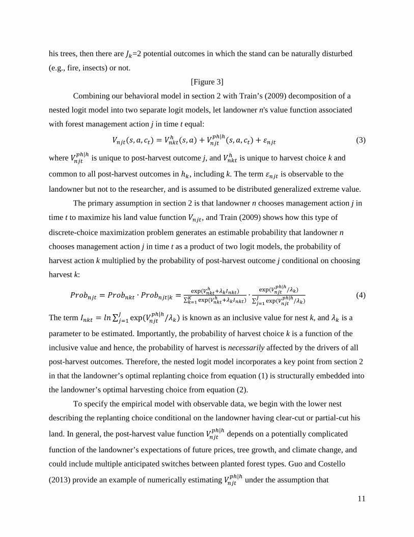
11

his trees, then there are 𝐽𝐽𝑘𝑘=2 potential outcomes in which the stand can be naturally disturbed

(e.g., fire, insects) or not.

[Figure 3]

Combining our behavioral model in section 2 with Train’s (2009) decomposition of a

nested logit model into two separate logit models, let landowner n's value function associated

with forest management action j in time t equal:

𝑉𝑉𝑛𝑛𝑗𝑗𝑡𝑡(𝑠𝑠,𝑎𝑎, 𝑐𝑐𝑡𝑡) = 𝑉𝑉𝑛𝑛𝑘𝑘𝑡𝑡ℎ (𝑠𝑠,𝑎𝑎) + 𝑉𝑉𝑛𝑛𝑗𝑗𝑡𝑡𝑝𝑝ℎ|ℎ(𝑠𝑠,𝑎𝑎, 𝑐𝑐𝑡𝑡) + 𝜀𝜀𝑛𝑛𝑗𝑗𝑡𝑡 (3)

where 𝑉𝑉𝑛𝑛𝑗𝑗𝑡𝑡𝑝𝑝ℎ|ℎ is unique to post-harvest outcome j, and 𝑉𝑉𝑛𝑛𝑘𝑘𝑡𝑡ℎ is unique to harvest choice k and

common to all post-harvest outcomes in ℎ𝑘𝑘, including k. The term 𝜀𝜀𝑛𝑛𝑗𝑗𝑡𝑡 is observable to the

landowner but not to the researcher, and is assumed to be distributed generalized extreme value.

The primary assumption in section 2 is that landowner n chooses management action j in

time t to maximize his land value function 𝑉𝑉𝑛𝑛𝑗𝑗𝑡𝑡, and Train (2009) shows how this type of

discrete-choice maximization problem generates an estimable probability that landowner n

chooses management action j in time t as a product of two logit models, the probability of

harvest action k multiplied by the probability of post-harvest outcome j conditional on choosing

harvest k:

𝑃𝑃𝑃𝑃𝑣𝑣𝑃𝑃𝑛𝑛𝑗𝑗𝑡𝑡 = 𝑃𝑃𝑃𝑃𝑣𝑣𝑃𝑃𝑛𝑛𝑘𝑘𝑡𝑡 ∙ 𝑃𝑃𝑃𝑃𝑣𝑣𝑃𝑃𝑛𝑛𝑗𝑗𝑡𝑡|𝑘𝑘 = exp (𝑉𝑉𝑛𝑛𝑛𝑛𝑛𝑛ℎ +𝜆𝜆𝑛𝑛𝐼𝐼𝑛𝑛𝑛𝑛𝑛𝑛)

∑ exp (𝑉𝑉𝑛𝑛𝑛𝑛𝑛𝑛ℎ +𝜆𝜆𝑛𝑛𝐼𝐼𝑛𝑛𝑛𝑛𝑛𝑛)𝐾𝐾

𝑛𝑛=1∙

exp (𝑉𝑉𝑛𝑛𝑛𝑛𝑛𝑛𝑝𝑝ℎ|ℎ/𝜆𝜆𝑛𝑛)

∑ exp (𝑉𝑉𝑛𝑛𝑛𝑛𝑛𝑛𝑝𝑝ℎ|ℎ/𝜆𝜆𝑛𝑛)𝐽𝐽

𝑛𝑛=1 (4)

The term 𝐼𝐼𝑛𝑛𝑘𝑘𝑡𝑡 = 𝑣𝑣𝑙𝑙 ∑ exp (𝑉𝑉𝑛𝑛𝑗𝑗𝑡𝑡𝑝𝑝ℎ|ℎ/𝜆𝜆𝑘𝑘)𝐽𝐽

𝑗𝑗=1 is known as an inclusive value for nest k, and 𝜆𝜆𝑘𝑘 is a

parameter to be estimated. Importantly, the probability of harvest choice k is a function of the

inclusive value and hence, the probability of harvest is necessarily affected by the drivers of all

post-harvest outcomes. Therefore, the nested logit model incorporates a key point from section 2

in that the landowner’s optimal replanting choice from equation (1) is structurally embedded into

the landowner’s optimal harvesting choice from equation (2).

To specify the empirical model with observable data, we begin with the lower nest

describing the replanting choice conditional on the landowner having clear-cut or partial-cut his

land. In general, the post-harvest value function 𝑉𝑉𝑛𝑛𝑗𝑗𝑡𝑡𝑝𝑝ℎ|ℎ depends on a potentially complicated

function of the landowner’s expectations of future prices, tree growth, and climate change, and

could include multiple anticipated switches between planted forest types. Guo and Costello

(2013) provide an example of numerically estimating 𝑉𝑉𝑛𝑛𝑗𝑗𝑡𝑡𝑝𝑝ℎ|ℎ under the assumption that

12

landowners dynamically optimize management under an anticipatory expectation of how climate

change will affect growth – and hence, profitability – from replanting different forest types.

However, evidence from extension research in the Pacific Northwest suggests that forest

landowners are currently not accounting for anticipated future climate change in their

management actions (Grotta et al. 2013); plus, forest landowners and appraisers in our study

region are specifically trained to estimate forestland values using a static expectations Faustmann

formula.5 Finally, large uncertainties in downscaled climate forecasting mean that “it is likely

that a great deal of climate adaptation will be reactive rather than anticipatory” (Massetti and

Mendelsohn 2018 p. 335).

In choosing which forest type to replant, landowners are assumed to compare the

expected rents that their land would generate when planted with different species. We specify

𝑉𝑉𝑛𝑛𝑗𝑗𝑡𝑡𝑝𝑝ℎ|ℎ for replanting (bottom left and center of figure 3) as a reduced-form function of the

average per-acre value function for planting species sj in region r that contains plot n, annualized

as a rent: 𝑃𝑃𝑟𝑟𝑙𝑙𝑟𝑟������𝑟𝑟(𝑛𝑛)𝑠𝑠𝑛𝑛𝑡𝑡, where the upper bar notation indicates a regional average. Regional rents

are a function of forest growth, forest type specific prices, and site productivity. To compute

expected rental values, the bare land values are first calculated for six forest types, seven site

productivity classes6, and eighteen price regions across the three states in our study region.7

Using the FIA data, we empirically fit separate yield curves for each forest type and site

productivity classes by price region, which are then used to compute approximate Faustmann

optimal rotation lengths. Rents are then imputed using a 5% discount rate (Appendix C).

A forest owner can select a forest type to replant from the following six types: (1)

Douglas-fir, (2) Fir/Spruce/Mountain hemlock, (3) Hemlock/Sitka spruce, (4) Ponderosa pine,

(5) Other softwoods8, and (6) Hardwoods9. One of the alternative specific constants is set to zero

for identification. We use observable variation in climate within each region to infer the

relationship between climate and replanting choice, using the revealed behavior of replanting

5 For example, Oregon State University Forestry Extension experts teach valuation techniques for small woodland owners using a textbook Faustmann formula. 6 The site productivity class ranges from 1 to 7, where 1 indicates the most productive plot. This is a classification of forest land in terms of inherent capacity to grow crops of industrial wood expressed in cubic feet/acre/year. 7 There are four sub-regions in Washington, five in Oregon, and nine in California, each corresponding to a price region for which state agencies report regional timber prices. 8 Other softwoods include lodgepole pine, redwood, western larch, western juniper, and numerous other pine species including knobcone, bishop, monterey, foxtail, limber, whitebark, and western white. 9 Major species of hardwoods are tanoak (CA and OR), red alder (OR and WA), bigleaf maple (OR and WA), black oak (CA), laurel (CA), canyon live oak (CA), pacific madrone (CA), white oak (OR), and cottonwood (WA).

13

choice. We do this by including interaction terms between our regional rents and the more

downscaled climate variables in the replanting equation. We specify the nested logit model for

the replanting nest as the following function:

𝑉𝑉𝑛𝑛𝑗𝑗𝑡𝑡𝑝𝑝ℎ|ℎ = 𝛽𝛽0𝑗𝑗

𝑝𝑝ℎ + 𝛾𝛾𝑝𝑝ℎ𝑃𝑃𝑟𝑟𝑙𝑙𝑟𝑟������𝑟𝑟(𝑛𝑛)𝑠𝑠𝑛𝑛𝑡𝑡 + 𝛽𝛽1𝑗𝑗𝑝𝑝ℎ𝑃𝑃𝑟𝑟𝑙𝑙𝑟𝑟������𝑟𝑟(𝑛𝑛)𝑠𝑠𝑛𝑛𝑡𝑡 ∙ 𝑐𝑐𝑛𝑛𝑡𝑡 + 𝛽𝛽2𝑗𝑗

𝑝𝑝ℎ𝑟𝑟𝑣𝑣𝑟𝑟𝑣𝑣𝑛𝑛 + 𝛽𝛽3𝑗𝑗𝑝𝑝ℎ𝑃𝑃𝑟𝑟𝑙𝑙𝑟𝑟������𝑟𝑟(𝑛𝑛)𝑠𝑠𝑛𝑛𝑡𝑡 ∙ 𝑐𝑐𝑛𝑛𝑡𝑡+30 (5)

𝑓𝑓𝑣𝑣𝑃𝑃 𝑝𝑝ℎ ∈ {𝑃𝑃𝑟𝑟𝑝𝑝𝑣𝑣𝑎𝑎𝑙𝑙𝑟𝑟|𝑐𝑐𝑣𝑣𝑟𝑟𝑎𝑎𝑃𝑃 − 𝑐𝑐𝑐𝑐𝑟𝑟, 𝑃𝑃𝑟𝑟𝑟𝑟𝑟𝑟𝑙𝑙𝑟𝑟𝑃𝑃𝑎𝑎𝑟𝑟𝑟𝑟|𝑝𝑝𝑎𝑎𝑃𝑃𝑟𝑟𝑝𝑝𝑎𝑎𝑣𝑣 − 𝑐𝑐𝑐𝑐𝑟𝑟}

where 𝑃𝑃𝑟𝑟𝑙𝑙𝑟𝑟������𝑟𝑟(𝑛𝑛)𝑗𝑗𝑡𝑡 and 𝑐𝑐𝑛𝑛𝑡𝑡 are rent and downscaled climate variables representing historical long-

run averages. Interactions between 𝑃𝑃𝑟𝑟𝑙𝑙𝑟𝑟������𝑟𝑟(𝑛𝑛)𝑗𝑗𝑡𝑡 and 𝑐𝑐𝑛𝑛𝑡𝑡 describe observable rent deviations

between plot n and the regional average; 𝑟𝑟𝑣𝑣𝑟𝑟𝑣𝑣𝑛𝑛 is the elevation of plot n, and 𝑐𝑐𝑛𝑛𝑡𝑡+30 is the

projected change in mean temperature based on the forecasted climate 30 years into the future.

Our inclusion of Faustmann rents into the specification of 𝑉𝑉𝑛𝑛𝑗𝑗𝑡𝑡𝑝𝑝ℎ is meant to provide a reasonable

and observable index for how prices, timber growth, and approximate expected rotation times

influence the post-harvest land value function, recognizing that landowners have many

unobservables (expectations, management skills, etc.) that also affect the value function and are

embedded in the logit unobservable, 𝜀𝜀𝑛𝑛𝑗𝑗𝑡𝑡. Similar to the logic of Severen et al. (2018), our

reduced form approach to including 𝑐𝑐𝑛𝑛𝑡𝑡+30 in equation (5) provides a simple test for whether

current economic decisions reflect a downscaled climate forecast in an anticipatory fashion.

The parameters for the interaction terms in (5) are specific to each replanting choice, thus

revealing the relationship between climate and the expected value of forestland associated with

each species replanted. Figure 4 graphically illustrates the intuition from this revealed preference

approach. The horizontal axis represents a climate measure (c) such as temperature. In figure

4(A), the climate is represented by a probability distribution, or the likelihood that each

temperature occurs. Figure 4(B) represents the relationship between the value of forestland and

climate. At 𝑐𝑐 ≤ 𝐶𝐶̅, planting Douglas-fir is optimal since the value of the land is highest in that

use, while planting (regenerating) hardwoods is optimal at 𝑐𝑐 > 𝐶𝐶̅. Since we do not observe plot-

level value functions of forestland, we instead use revealed planting choices at the current

climate distribution f1 to estimate parameters in (5) which then generate the probability of

replanting a forest type as a function of climate c. If the climate distribution shifts from f1 to f2 in

figure 4, then our estimated model would predict an increase in probability that landowners will

plant hardwoods with a corresponding decrease in the probability of planting Douglas-fir (i.e.,

PD2<PD1 in figure 4).

[Figure 4]

14

We account for the risk of natural disturbance in estimation through the “no-cut” nest

(bottom right of figure 3), where landowners refrain from cutting their timber in exchange for

letting the trees grow an additional period. By choosing not to cut, the landowner leaves the

stand at risk to the binary outcomes of natural disturbance or no disturbance. Since fire risk

influences the landowner’s harvest decision (Reed 1984), we jointly estimate drivers of

disturbance and harvest decisions by specifying the nested logit model for the lower “no-cut”

nest as a binary model:

𝑉𝑉𝑛𝑛𝑗𝑗𝑡𝑡𝑝𝑝ℎ|ℎ = 𝜔𝜔0

𝑝𝑝ℎ + 𝜔𝜔1𝑝𝑝ℎ𝑝𝑝𝑃𝑃𝑝𝑝𝑣𝑣𝑛𝑛 + 𝜔𝜔2

𝑝𝑝ℎ𝑟𝑟𝑣𝑣𝑟𝑟𝑣𝑣𝑛𝑛 + 𝜔𝜔3𝑝𝑝ℎ𝑠𝑠𝑝𝑝𝑟𝑟𝑐𝑐𝑝𝑝𝑟𝑟𝑠𝑠𝑛𝑛𝑡𝑡 + 𝜔𝜔4

𝑝𝑝ℎ𝑣𝑣𝑣𝑣𝑣𝑣𝑛𝑛𝑡𝑡 + 𝜔𝜔5𝑝𝑝ℎ𝑐𝑐𝑛𝑛𝑡𝑡 + 𝜔𝜔6

𝑝𝑝ℎ𝑠𝑠𝑟𝑟𝑎𝑎𝑟𝑟𝑟𝑟𝑛𝑛

(6)

𝑓𝑓𝑣𝑣𝑃𝑃 𝑝𝑝ℎ ∈ {𝑑𝑑𝑝𝑝𝑠𝑠𝑟𝑟𝑐𝑐𝑃𝑃𝑃𝑃𝑎𝑎𝑙𝑙𝑐𝑐𝑟𝑟 𝑟𝑟𝑣𝑣𝑟𝑟𝑙𝑙𝑟𝑟|𝑙𝑙𝑣𝑣 − 𝑐𝑐𝑐𝑐𝑟𝑟}

The independent variables include an ownership dummy indicating private or state ownership

(𝑝𝑝𝑃𝑃𝑝𝑝𝑣𝑣𝑛𝑛), elevation (𝑟𝑟𝑣𝑣𝑟𝑟𝑣𝑣𝑛𝑛), forest type dummy variables indicating the forest type (𝑠𝑠𝑝𝑝𝑟𝑟𝑐𝑐𝑝𝑝𝑟𝑟𝑠𝑠𝑛𝑛), the

current timber volume (𝑣𝑣𝑣𝑣𝑣𝑣𝑛𝑛𝑡𝑡), a state dummy (𝑠𝑠𝑟𝑟𝑎𝑎𝑟𝑟𝑟𝑟𝑛𝑛), and a vector of climate variables (𝑐𝑐𝑛𝑛𝑡𝑡).

Climate variables such as precipitation directly affect nature’s ability to suppress fires, while

other climate variables such as minimum winter temperatures can affect the susceptibility of

certain trees to damage. We do not have data on past fire management activities for each plot

(e.g., thinning, controlled burns, etc.), which end up in the econometric unobservable. Our

current specification assumes that unobserved fire management activities are uncorrelated with

the independent variables in (6).

Now consider the upper nest in figure 3, whereby the forest landowner makes the harvest

decision by choosing whether to clear-cut, partial-cut, or not cut his stand of trees. Following

Provencher (1997), we specify the observable components specific to the net revenue from

harvest method h as:

𝑉𝑉𝑛𝑛𝑘𝑘𝑡𝑡ℎ = 𝛼𝛼0𝑘𝑘 + 𝛼𝛼1𝑘𝑘𝑃𝑃𝑛𝑛𝑠𝑠𝑛𝑛𝑡𝑡 ∙ 𝑣𝑣𝑣𝑣𝑣𝑣𝑛𝑛𝑘𝑘�𝑠𝑠𝑛𝑛�𝑡𝑡ℎ (7)

𝑓𝑓𝑣𝑣𝑃𝑃 ℎ ∈ {𝑐𝑐𝑣𝑣𝑟𝑟𝑎𝑎𝑃𝑃 − 𝑐𝑐𝑐𝑐𝑟𝑟,𝑝𝑝𝑎𝑎𝑃𝑃𝑟𝑟𝑝𝑝𝑎𝑎𝑣𝑣 − 𝑐𝑐𝑐𝑐𝑟𝑟}

And we specify the observable components specific to the decision not to cut and let the stand

grow as a function of expected changes in revenue:

𝑉𝑉𝑛𝑛𝑘𝑘𝑡𝑡ℎ = 𝛼𝛼1𝑘𝑘𝑃𝑃𝑛𝑛𝑠𝑠𝑛𝑛𝑡𝑡 ∙ ∆𝑣𝑣𝑣𝑣𝑣𝑣𝑛𝑛𝑘𝑘(𝑠𝑠𝑛𝑛)𝑡𝑡 (8)

𝑓𝑓𝑣𝑣𝑃𝑃 ℎ ∈ {𝑙𝑙𝑣𝑣 𝑐𝑐𝑐𝑐𝑟𝑟}

In this specification, we use observable time t timber prices for forest type sj from the region that

contains plot n, and multiplied by the observable species sj timber volume for management

15

choice k as a representation of the one-time revenue that the landowner would receive from

picking harvest choice k. Since clear cutting necessarily entails harvesting more volume than

partial cutting10, the volume variable is indexed by harvest choice k. The post-harvest value

function from not-cutting the land – 𝑉𝑉𝑡𝑡+1𝑝𝑝ℎ|𝑁𝑁𝐶𝐶(𝑠𝑠,𝑎𝑎 + 1, 𝑐𝑐𝑡𝑡+1) in equation (2) – is affected by the

marginal benefit of waiting to cut, which is the change in revenue that could be received by

allowing the stand to grow an additional period.11

Finally, the nested logit structure embeds the inclusive value 𝐼𝐼𝑛𝑛𝑘𝑘𝑡𝑡 of the lower post-

harvest nests into the upper harvest nest of the estimated probabilities in equation (4). For the

two harvest alternatives (clear-cut and partial-cut), 𝐼𝐼𝑛𝑛𝑘𝑘𝑡𝑡 approximates the optimized post-harvest

land value associated with picking the forest type to replant (Hartman 1988; Train 2009), which

is a direct measure of the solution to equation (1).12 With the inclusive value from each nest,

climate implicitly affects the harvest decision and so this empirical framework allows the climate

to affect adaptation on the extensive margin (choosing which forest type to plant) and on the

intensive margin (altering the harvest time). The alternative specific constant of “no-cut” is

normalized to zero.

The parameters defining the probabilities of harvest, disturbance, and replanting choices

are simultaneously estimated with maximum likelihood techniques using original MATLAB

code. The log-likelihood function is:

𝐿𝐿𝐿𝐿(𝛼𝛼,𝛽𝛽, 𝛾𝛾, 𝜆𝜆) = ∑ ∑ 𝑦𝑦𝑛𝑛𝑗𝑗 𝑣𝑣𝑙𝑙 𝑃𝑃𝑃𝑃𝑣𝑣𝑃𝑃𝑛𝑛𝑗𝑗𝑡𝑡𝑗𝑗𝑛𝑛 (9)

where 𝑦𝑦𝑛𝑛𝑗𝑗 equals one if landowner n chooses management j. We index some variables in the

model with time t to represent that different plots are observed at different points in time, and so

different plots have variables measured at different points in time. This is a pooled rather than a

10 Partial cut volume is estimated by comparing the measured volumes in 10-year intervals for the re-measured plots that have a record of partial cut treatment in the most recent survey. For the other plots, we assigned the percentage of partial cut portion of total volume according to the available information such as the treatment code that distinguishes “less than 20% removed” or “more than 20% removed”, as well as county average percentage across the re-measured partially-cut plots. 11 We use radial ten-year increment data on tree growth for each FIA plot to construct an approximation of plot-specific tree growth – Δ𝑣𝑣𝑣𝑣𝑣𝑣𝑛𝑛𝑘𝑘(𝑠𝑠𝑛𝑛)𝑡𝑡 – which when multiplied by 𝑃𝑃𝑛𝑛𝑠𝑠𝑛𝑛𝑡𝑡 provides us with a direct measure of the marginal benefit of waiting to cut (see Appendix D for more details). 12 The inclusive value for the “no-cut” nest implicitly accounts for the risk of disturbance on the harvest decision, although this inclusive value is harder to interpret than in the clear-cut and partial-cut nests since the outcomes from choosing not to cut (natural disturbance or not) are not a direct choice by the landowner. Therefore, the inclusive values from the disturbance nest may not be justified as the utility gained by optimally choosing the best alternative, nor satisfy the consistency condition for utility maximization (Herriges and Kling 1996). See section 4.2 for robustness checks for specifying the no-cut nest.

16

panel data model.13 Finally, we weight each plot’s likelihood by the expansion factor assigned in

the FIA database, where the expansion factor represents the sampling intensity associated with

the sample plots.

If a plot is naturally disturbed with wildfire, we use historical spatial-temporal data on

wildlife burn severity to separately estimate a burn severity index as a function of the same

climate and other plot level drivers of natural disturbance from equation (6):

𝑆𝑆𝑉𝑉𝑛𝑛 = 𝐺𝐺(𝑝𝑝𝑃𝑃𝑝𝑝𝑣𝑣𝑛𝑛, 𝑟𝑟𝑣𝑣𝑟𝑟𝑣𝑣𝑛𝑛, 𝑠𝑠𝑝𝑝𝑟𝑟𝑐𝑐𝑝𝑝𝑟𝑟𝑠𝑠𝑛𝑛𝑡𝑡, 𝑣𝑣𝑣𝑣𝑣𝑣𝑛𝑛𝑡𝑡, 𝑐𝑐𝑛𝑛𝑡𝑡, 𝑠𝑠𝑟𝑟𝑎𝑎𝑟𝑟𝑟𝑟𝑛𝑛; 𝝑𝝑) (10)

where 𝑆𝑆𝑉𝑉𝑛𝑛 is the most dominant burn severity (1: unburned to low, 2: low, 3: moderate, or 4:

high) that has occurred in the last ten years within a 2km radius around each plot. The vector of

parameters 𝝑𝝑 are estimated as an ordered logit model (see Appendix E) using historical burn

severity data from 2001-2014. The parameters defining the probabilities of burn severity are

estimated outside of the nested logit framework, as coupling an ordered logit model to the nested

logit model is computationally challenging and brings up convergence concerns. Estimating burn

severity parameters separately means that we are not accounting for how variation in the burn

severity level will affect land value and management. Instead, we use the projected probabilities

of severity in the simulation (see sec. 5) to adjust the stand volume, age, and incremental growth.

3.2 Data

We have plot-level data from FIA for over 6,800 forested plots with variables representing forest

type, site quality, tree growth, elevation, an indication of recent harvest, and an indication of

recent natural disturbance. We combine the plot-level forest management data with downscaled

climate data and regional timber prices that vary across forest types and site quality. The study

area of Oregon, Washington, and California has a substantial portion of its landscape dedicated

to commercial forest production (30%, 44%, and 45% of non-federal rural lands are forested in

California, Oregon, and Washington, respectively), including some of the most productive

forests in the world, and has considerable climate variation and corresponding variation in forest

13 An alternative approach to estimation would be to set up a dynamic discrete choice model (e.g., Provencher 1995). However, while we can set up the harvest nest as a panel of repeated decisions, we only observe replanting decisions when the landowner has chosen to harvest (once for those that harvest between 2001 and 2014, never for those that don’t harvest between 2001 and 2014). Thus, our data does not include temporal changes in the key explanatory variables of interest (climate) or panel data in the key behavioral variable of interest (replanting) that would make dynamic discrete choice estimation more informative than our current approach (Aguirregabiria and Mira 2010).

17

types (figure 5.a). Due to a methodological change in data collection, the FIA is only available

since 2001. Since we don’t observe multiple harvests on the same plot, a complete set of panel

data does not exist14.

[Figure 5]

Each plot is designed to cover 1-acre and is randomly sampled. Plot locations are slightly

“fuzzed” for confidentiality in that each plot’s true location is within at most 1 mile (1.6 km) of

its stated location. Using a national standard for field measurements for a wide range of site

attributes, the FIA presents the most detailed plot-level data available for our purposes.15 The

key dependent variables for econometric analysis include a qualitative indicator of harvest on an

FIA plot (clear-cut, partial-cut, no-cut), the forest type replanted upon harvest, and the presence

of a natural disturbance (e.g., fire, insect damage, etc.). The plot-level attributes used include

forest type, stand volume, incremental volume growth, owner type, stand age, and elevation. We

assigned each plot to a specific timber price region for different forest types. Historical timber

prices for different grades are drawn from records available by state-level agencies. Since not all

forest types can physically grow across the entire region, each plot is assigned a choice set based

on the “plant viability scores” developed by the USDA Forest Service that reflects the likelihood

that the climate at a given location would be suitable for each species (Crookston et al. 2010).16

The climate variables observable to the landowners are total precipitation and mean

temperature during the growing season17, the maximum temperature in the warmest month

(August), and minimum temperature in the coldest month (December). These variables have

been found to be some of the most influential variables that affect the growth of trees (Rehfeldt

et al. 2014). Plot-level climate data is based on normal monthly data from the Parameter-

elevation Regressions on Independent Slopes Model (PRISM) at 800m resolution over a 30-year

14 FIA surveys a fraction of all plots (10%) every year. Therefore, re-measurements occur every 10 years. For those re-measured, dependent variables reflect data from both measurements over 10-year timeframe. 15 Remote sensing data neither distinguishes different tree species nor detailed site characteristics. 16 Viability score values near zero indicate a low suitability while those near 1.0 indicate a suitability so high that the species is nearly always present in that climate. Although the score below 0.5 indicates little chance of survival, we use the score of 0.3 as a cut-off point whether the species is included in a choice set, to account for the error disclosed in Crookston et al. (2010). 17 Growing season months are those that have growing degrees days above 10 C° (50F), which are determined at a regional level that represents varying climate zones. Regional climate data is from National Oceanic and Atmospheric Administration (NOAA) National Climatic Data Center.

18

period between 1981 and 2010. The climate projection that we use is of high spatial resolution

(1km) and is easily available to the public online.18

Appendix F presents a full list of data sources and summary statistics of the data, but a

few highlights are covered here. First, 9.3% (5.6%) of forest plots were clear-cut (partial-cut)

over the ten-year sample period for each plot. Second, on a per-unit basis, Douglas-fir logs were

the most commercially valuable forest type ($458.50/MBF) and comprise about 50% of total

harvested volume, and hardwoods are the least valuable ($254.49/MBF). Third, Douglas-fir and

hemlock/sitka spruce are more commonly harvested by clear-cut in the wetter region west of the

major mountain ranges, while ponderosa pine is more commonly harvested by partial-cut in the

drier region east of the major mountain ranges. Finally, fir/spruce forest types are most

commonly found in the mountains at high elevation while hardwoods are most commonly found

in the valleys at a lower elevation.

4. Econometric Estimation Results

The full set of nested logit parameter estimates and partial effects for key variables are presented

in Appendix G. Parameter estimates (Table G1) show that replanting decisions and natural

disturbance are significantly affected (p<0.05) by a variety of climate variables, and generally

conform to expectations and yield four general conclusions. First, in the lower replanting nest,

the estimated coefficient on the rent variable is positive and highly significant (p<0.01) as

expected - landowners are more likely to replant forest types that are more profitable. Second,

the rent-climate interaction parameters are jointly significant in the replanting nest (p<0.01) but

individual parameters are highly variable in magnitude and statistical significance across the

different replanting choices. About 40% of the individual climate parameters are significantly

different from zero. Third, natural disturbance is more likely on high elevation, large volume,

and dry plots that experience cold winter temperatures and that are hardwood or “other

softwood” forest type. Fourth, in the upper harvest nest, the estimated coefficients are

significantly different from zero (p<0.05) and consistent with standard comparative statics from

harvesting models – a timber harvest is more likely when the marginal costs of waiting to harvest

are high (i.e., harvest revenue; inclusive value proxy for optimized bare land value), and less

likely when the marginal benefits of waiting to harvest are high (i.e., growth in harvest revenue). 18 The downscaled data at 1km resolution was obtained from the ClimateWNA model developed by the Center for Forest Conservation Genetics at the University of British Columbia (Wang et al. 2012), which is available at https://adaptwest.databasin.org/pages/adaptwest-climatena.

19

A notable partial effect (Table G2) is that the probability of replanting Douglas-fir

declines by approximately 30 percentage points given a 3 C° increase in mean temperature

(p<0.01) for the prime growing regions of western Oregon and Washington – a direct estimate of

PD2-PD1 from Fig. 4. We find limited evidence that our variables representing future 30-year

forecasts of mean temperature significantly affect replanting. The partial effect of a 1 C° increase

in forecasted future mean temperature has no significant effect on the probability of replanting

all forest types except ponderosa pine, where the partial effect is -8.2% and only marginally

significant (p<0.1). Thus, we find strong evidence that current replanting decisions react to

current climate, but limited evidence that current replanting decisions respond to anticipated

forecasts of future climate.

The partial effect of rent on the probability of replanting each forest type is the primary

mechanism that we use to simulate the impacts of a carbon rental payment on forest composition.

Given our use of interactions between regional rents and downscaled climate variables in

equation (5), the partial effects of replanting with respect to rent depend on climate. Figure 6

shows the partial effect of rent on replanting two main forest types in the region – Douglas-fir

and hardwoods. As seen in figure 6.a and 6.b, the average partial effects of rent on replanting

Douglas-fir fall with climate change, while the average partial effects of rent on replanting

hardwoods are roughly the same with climate change. By basing estimation off landowners’

revealed preferences for replanting forest types at locations with different current climates, the

estimated partial effects pick up the declining productivity of Douglas-fir with the warming

climate that we hypothesized in the conceptual relationship from figure 4. As a check on this

important finding, we compare our estimated partial effects to natural science projections of the

biophysical viability of Douglas-fir and hardwoods from Crookston et al. (2010) where higher

viability scores indicate higher viability.19 Figure 6.c and 6.d show average viability scores for

Douglas-fir and hardwood forest types for our study region as a function of the climate

projections. Both the econometric model and the natural science model produce results

indicating strong declines in the productivity of Douglas-fir with the warmer climate. Hardwoods

become somewhat less viable in the natural science model, while the econometric results show

no strong decline in productivity. The similar impact of climate on both the econometric partial

effects and the biophysical viability scores provides a qualitative convergent validity check. 19 We thank Crookston for providing us with plot-level viability scores for our study region. Appendix H shows maps of viable plots for Douglas-fir and hardwoods across the Pacific states.

20

[Figure 6]

Finally, Appendix I presents results from nine sets of robustness checks of the

econometric model, which indicate that the model is quite robust to alternative specifications.

5. Landscape Simulation Analysis

On their own, the parameter and marginal effect estimates from the econometric model do not

give a full picture of the potential landscape shifts under climate change. Replanting does not

occur continuously, but only after infrequent harvest events (~15% probability of a plot being

harvested over 10 years). The projected climate changes are also heterogeneous across plots.

And since multiple climate variables will shift in a spatially heterogeneous fashion

simultaneously, simulating the combined effects when all climate variables shift at the same time

will render more informative results. A landscape simulation will need to take these factors into

consideration in order to examine the effect of a path of climate changes on landscape change.

As described in section 1, we use our econometrically estimated forest management and natural

disturbance probabilities as a set of decision rules to simulate multiple realizations of changes in

the landscape of forest types under a changing climate and a carbon price policy.

5.1 Simulated climate change and carbon pricing scenarios

We simulate three scenarios of landscape change. First, the baseline scenario assumes no climate

change or carbon price and simply extends the observed forest management practices from 2001

to 2014 into the future. Second, the climate change only scenario assumes future climate regimes

are derived from the U.S. National Center for Atmospheric Research Community Climate

System Model (CCSM) 420. Out of the available scenarios included in the model, we chose the

RCP 8.5 scenario, as current CO2 emission rates are closely tracking this pathway (Sanford et al.

2014; McKenney et al. 2015). Under the RCP 8.5 scenario, the majority of premier private

forestland in the west side of the Cascades, the area shown in brown in figure 5.b, is expected to

become warmer and drier. The average temperature is expected to increase by 4.35 ºC by 2100

on average in the study region.

In the carbon pricing scenario, we use the RCP 8.5 climate projection and add a

hypothetical carbon pricing scheme. Our carbon pricing scheme starts in 2020 and assumes 20 CCSM4 climate model is ranked as one of the best of 41 Global Climate Models (GCM) as to the credibility of predicting the future climate according to the models’ abilities to reproduce the observed metrics (Rupp et al. 2013). We also simulated the landscape using an alternative climate projection of an ensemble of 15 GCMs instead of using one GCM, but the results show little changes from our original results.

21

landowners receive rental payments for the amount of carbon sequestered in their forests. We

assume that a carbon price starts at $15/ton in 2020, rises to $50 in 2050, and again to $80 in

2080. To determine carbon payment values to landowners, we estimate regional average carbon

yield curves from the FIA data, where tons of carbon sequestered is expressed as a function of

stand age. The carbon yield curves vary by forest type, region, and site class. Given a set of

timber prices, carbon prices and yield functions for each region r, we translate the carbon price to

a regional average per-acre rental payment for each plot n that is in region r and is planted with

species 𝑠𝑠𝑗𝑗 (𝑃𝑃𝑟𝑟𝑙𝑙𝑟𝑟������𝑟𝑟(𝑛𝑛)𝑠𝑠𝑛𝑛𝑇𝑇𝐶𝐶 ), where the “TC” superscript indicates that landowners are being paid for

both timber and carbon sequestration. We calculate 𝑃𝑃𝑟𝑟𝑙𝑙𝑟𝑟������𝑟𝑟(𝑛𝑛)𝑠𝑠𝑛𝑛𝑇𝑇𝐶𝐶 using the approach of van Kooten

et al. (1995), which subsidizes landowners for carbon sequestered through tree growth while

taxing landowners for carbon released at harvest.21 We calculate 𝑃𝑃𝑟𝑟𝑙𝑙𝑟𝑟������𝑟𝑟(𝑛𝑛)𝑠𝑠𝑛𝑛𝑇𝑇𝐶𝐶 under the assumption

that landowners solve for the rotation length that maximizes the present value of timber and

carbon benefits. The carbon price scenario is implemented by replacing the variable 𝑃𝑃𝑟𝑟𝑙𝑙𝑟𝑟������𝑟𝑟(𝑛𝑛)𝑠𝑠𝑛𝑛𝑡𝑡

(timber rents only) in the lower replanting nests in equation (5) with 𝑃𝑃𝑟𝑟𝑙𝑙𝑟𝑟������𝑟𝑟(𝑛𝑛)𝑠𝑠𝑛𝑛𝑇𝑇𝐶𝐶 (timber and

carbon rents). This approach assumes that a landowner is indifferent between $1 in carbon rent

and $1 in timber rent. The value of 𝑃𝑃𝑟𝑟𝑙𝑙𝑟𝑟������𝑟𝑟(𝑛𝑛)𝑠𝑠𝑛𝑛𝑇𝑇𝐶𝐶 reflects the regional average timber and carbon

rent at today’s climate distribution. The effects of climate change on timber and carbon rents are

accounted for by the econometric parameters in (5), which translates any given combination of

𝑃𝑃𝑟𝑟𝑙𝑙𝑟𝑟������𝑟𝑟(𝑛𝑛)𝑠𝑠𝑛𝑛𝑇𝑇𝐶𝐶 and climate 𝑐𝑐𝑛𝑛𝑡𝑡 for each plot n to forest management probabilities. As discussed in

section 4, our econometric results imply that the average Douglas-fir plot is becoming less

productive under climate change in western Oregon and Washington, and thus the econometric

model implicitly lowers the carbon sequestration productivity of the average Douglas-fir plot

under the assumed RCP 8.5 climate change path.

Differences between the climate change only scenario and the baseline give us the impact

of climate change on the resulting landscape. Differences between the carbon pricing scenario

21 Some have argued that carbon rents in forestry should account for the issue of additionality: pay only for the amount of carbon that would not have been sequestered without the carbon pricing policy. Additionality payments have a basic problem stemming from asymmetric information, which is that only the seller knows whether she would have undertaken the activity in the absence of a payment for the offset (Mason and Plantinga 2013). Implementing additionality payments in forest management presents challenging tradeoffs between efficiency and budget concerns; recent work has proposed the use of a general land tax (Tahvonen and Rautiainen 2017) but has not considered how to implement the mechanism in a model where landowners can alter their replanting choice. Incorporating additionality into our model of replanting choices is beyond the present scope of our analysis.

22

and the climate change only scenario give us the impact of carbon pricing alone, while the

difference between the carbon pricing scenario and the baseline gives us the combined impact of

climate change and carbon pricing.

Future timber prices are projected to increase by 0.4% and 0.5% per year under the

climate change scenario and baseline scenario, respectively, using results from Sohngen and

Tian’s (2016) global timber model.22 To adjust the forest growth functions to projected climate

change, we adapt the net primary productivity (NPP) projection for Douglas-fir developed by

Nicholas Coops and Richard Waring in their 3-PG process model (Coops et al. 2010). As shown

in Appendix J, NPP is expected to decline relative to the 1990 level in most of the west side of

the study region and increase in most of the east side. For each plot, incremental tree growth at

each future time step is adjusted by multiplying the incremental tree growth with the downscaled

NPP at each location and at each time step relative to NPP in the base year (e.g., if NPP in 2020

is 30 and NPP in 1990 is 32, relative NPP is 30/32 = 0.93). Regional timber rents are also

adjusted to reflect the biophysical effects of climate on NPP.

5.2 Summary of key assumptions that drive the landscape simulation

Our simulation uses the estimated plot-level management probabilities to project changes

in the U.S. Pacific coast forest stock by simulating and aggregating plot-level management and

natural disturbance outcomes in response to a number of exogenously changing variables. We

assume that climate exogenously changes under RCP 8.5 and that global timber prices and the

NPP of forests change in response to climate change as estimated by Sohngen and Tian (prices)

and Coops et al. (NPP). Within the simulation, the estimated management/disturbance

probabilities from our discrete-choice model determine how the timing and intensity of harvest,

the forest type to replant, and natural disturbance respond to the exogenously changing variables

within multiple 10-year time steps. Our estimated econometric model imposes an assumption

that landowners have static expectations of exogenous factors – in time t, landowners assume

that the level of the exogenous variables (climate, prices, NPP) will continue indefinitely at

period t levels.23 Since the simulation operates at 10-year time-steps, then landowners respond to

changes in the exogenous factors and re-optimize their management decisions every 10 years. 22 Sohngen and Tian project that forest prices rise more slowly with climate change, largely because climate change is expected to increase overall global forest productivity. 23 The static expectations assumption is relaxed somewhat by our inclusion of mean temperature forecasts in the replanting nests and the simulation. However, as discussed in section 4.1, our econometric estimates find only limited evidence that current replanting decisions respond to future mean temperature forecasts.

23

For example, the estimated rental value for Douglas-fir that determines the probability of

replanting Douglas-fir in 2060 is a function of the constant levels of all exogenous variables that

occur in 2060 (climate, prices, NPP), which are different than the exogenous variable levels that

were used to calculate the same Douglas-fir rental value in 2020. Our simulation approach

implicitly implements Massetti and Mendelsohn’s (2018) argument that climate adaptation will

be reactive rather than anticipatory, with people adjusting to the changes in climate that they

actually observe. Previous large-scale econometric landscape simulation exercises have operated

under similar assumptions about expectations (e.g., Lubowski et al. 2006; Lawler et al. 2014). In

contrast, market simulation analyses of forestry assume that markets perfectly anticipate future

climate change (e.g., Sohngen and Mendelsohn 1998; Lee and Lyon 2004).

5.3 Landscape changes under baseline, climate change, and carbon pricing scenarios

For each scenario, we calculate the average share of non-federal forestland in each forest type

and for each time step, averaged over the 1,000 Monte Carlo simulated landscape outcomes.

Figure 7 presents our projection of each forest type’s composition in California, Oregon, and

Washington for the baseline, climate change, and carbon pricing scenarios.

[Figure 7]

Examining the three scenarios provides three conclusions. First, climate change induces a

reduction in the share of non-federal forestland in the commercially-dominant Douglas-fir type

in Oregon and Washington and induces an increase in the share of ponderosa pine (for

California) and hardwoods (all states)24. Second, carbon pricing reinforces these shifts. Third, the

extent of landscape change is subtle since replanting harvested land – thus replacement of a

landscape’s forest type – occurs gradually on a fraction of the landscape following infrequent

harvest events. The seemingly subtle landscape change is masking a change in replanting

preference that is happening much more drastically. For example, figure 8 shows that while 50%

of all harvested land in Oregon is currently replanted with Douglas-fir, only 16% of harvested

land in Oregon is projected to be replanted to Douglas-fir by 2090 under climate change and

carbon pricing. This is a sizable shift in the preference for the most commercially dominant tree

in the Pacific Northwest. In contrast, hardwoods currently comprise 12% of

24 This is consistent with current advice from Oregon State University Extension Service, which recommends that landowners should consider planting ponderosa pine or hardwoods where Douglas-fir mortality is occurring in western Oregon (Oregonian/OregonLive 2018).

24

replanting/regeneration on harvested land in Oregon, but that share rises to 53% by 2090 under

climate change and carbon pricing.

[Figure 8]

Figure 9 highlights regional differences for the two forest types that experience the

largest changes – Douglas-fir and hardwoods. We compare total landscape change over the

whole period as well as change on harvested plots only in the final period (2090 to 2100).

Compared to the landscape change, landowners dramatically increase the replanting of

hardwood species on harvested land in 2090 at the expense of Douglas-fir in Oregon and

Washington in particular – a region that is mostly predicted to become warmer and drier under

the climate scenario we use. Both climate change and carbon pricing induce the shift from

Douglas-fir to hardwoods. As discussed in section 4, Douglas-fir gets less productive under

climate change, as reflected by the declining estimated partial effect of rent on replanting

Douglas-fir with the warming climate. Since most Douglas-fir plots in our region are artificially

regenerated by planting, while most hardwoods are naturally regenerated following harvest, a

switch from Douglas-fir to hardwoods could be interpreted as landowners abandoning the

management intensive form of artificial regeneration (replanting) of Douglas-fir in favor of less

management-intensive natural regeneration of hardwoods.

[Figure 9]

5.4 Probability of changing forest types (extensive margin adaptation)

The above simulation results are averages across 1,000 simulated landscape changes. The speed

of landscape change is driven by the magnitude of harvest and natural disturbance in each 10-

year period, while the direction of change is driven by the replanting/regeneration choices. To

exploit further information in the estimated probabilities of forest management, we calculate the

effects of climate change and carbon prices on the probability that landowners change from their

initial forest types to a different forest type by 2100. We interpret this measure as a probability of

adaptation on the extensive margin. For plot n that begins today in forest type 𝑠𝑠𝑖𝑖, the simulations

generate 1,000 realizations of plot n’s forest type by the year 2100. The probability of extensive

margin adaptation for plot n is defined as 𝑃𝑃𝑃𝑃𝑣𝑣𝑃𝑃𝑛𝑛(𝑎𝑎𝑑𝑑𝑎𝑎𝑝𝑝𝑟𝑟) = [1 − 𝑃𝑃𝑃𝑃𝑣𝑣𝑃𝑃𝑛𝑛�𝑠𝑠𝑖𝑖,2100 = 𝑠𝑠𝑖𝑖,2010�],

which is calculated as the proportion of the 1,000 simulations in which plot n ends the year 2100

in a different forest type than it began in 2010. Subtracting the baseline calculation of

𝑃𝑃𝑃𝑃𝑣𝑣𝑃𝑃𝑛𝑛(𝑎𝑎𝑑𝑑𝑎𝑎𝑝𝑝𝑟𝑟) from the climate change calculation of 𝑃𝑃𝑃𝑃𝑣𝑣𝑃𝑃𝑛𝑛(𝑎𝑎𝑑𝑑𝑎𝑎𝑝𝑝𝑟𝑟) gives the discrete effect

25

of a 90-year climate path on the probability of adaptation. Similarly, subtracting the climate

change calculation of 𝑃𝑃𝑃𝑃𝑣𝑣𝑃𝑃𝑛𝑛(𝑎𝑎𝑑𝑑𝑎𝑎𝑝𝑝𝑟𝑟) from the carbon pricing scenario version of 𝑃𝑃𝑃𝑃𝑣𝑣𝑃𝑃𝑛𝑛(𝑎𝑎𝑑𝑑𝑎𝑎𝑝𝑝𝑟𝑟)

gives the discrete effect of a 90-year carbon price path on the probability of adaptation. Table 1

presents results for western Oregon and Washington as an example, differentiated by initial

forest type and final forest type. A full table for all regions is included in Appendix K.

[Table 1]

Table 1 shows that the discrete effect of a 90-year path of climate change and carbon

pricing varies across regions and initial forest types. For example, a Douglas-fir landowner in

western Oregon is 10.6% more likely to adapt away from Douglas-fir on the extensive margin by

the year 2100 under climate change. In contrast, the current owner of a hardwoods plot in

western Oregon is 16.5% less likely to adapt to another forest type by 2100 under climate

change. A key result from Table 1 is that both a carbon price and climate change increase the

probability that Douglas-fir owners in the prime-growing regions of western Oregon and

Washington adapt to another forest type by the year 2100. Looking at the final forest types that

the landowners are switching to, we find that the 90-year path of a carbon price has an effect

similar to climate change – especially favoring hardwoods at the expense of Douglas-fir.

6. Discussion

The purpose of this paper is to quantify the effect of climate change and carbon pricing on the

adaptation behaviors of private forest owners. While much attention focuses on climate change

as a source of damage to human well-being, we focus on the fact that climate change is also an

important input to many decisions, including forest management, and that adaptive decisions can

induce changes to natural resource stocks that can cause changes in human well-being.

Adaptation behavior in forestry affects landscapes directly, leading to a change in forest

composition, which can then alter the flow of ecosystem services from forests. In order to

understand the impact of climate change on landscape outcomes, we need to account for how

landscape change is affected by deliberate adaptive decisions in response to climate, which in the

case of forestry is also affected by policy interventions that aim to mitigate climate change. Our

paper uses empirical evidence and simulation techniques to examine how climate adaptation,

mitigation, and natural resources interact through land-use change. An important finding is that

along the U.S. Pacific coast, landowners adapt to climate change by gradually shifting out of

26

their current dominant species choice of Douglas-fir to species more suitable for the future

climate, notably hardwoods and ponderosa pine.

Our findings also show that carbon pricing accelerates forest landowners’ adaptation

behaviors to climate change, reinforcing the forest landscape shift away from coniferous

Douglas-fir forest types to other types such as hardwoods. The carbon price rewards the climate-

induced relative shift in productivity away from Douglas-fir to hardwoods. A clear shift that

involves two distinctively different forest types indicates that we should likely expect habitat

losses for wildlife species that are specialized to Douglas-fir habitat, and future habitat gains for

wildlife species that are specialized to hardwood forests. State wildlife agencies along the U.S.

Pacific coast recognize many wildlife species of conservation concern that are specialized to

both coniferous forests25 and hardwood forests26, and these species of conservation concern are

sensitive to changes in private forests. Future research could link our projections of landscape

change under climate change and carbon pricing with more detailed assessments of the spatial

pattern and range of habitats for wildlife of conservation concern. Nevertheless, our results

suggest that carbon pricing generates tradeoffs between choices that are privately optimal to

landowners against non-market changes in forest ecosystem services that may generate social

costs to non-landowners. This unintended effect of carbon pricing can lead to wildlife and

biodiversity outcomes that have the potential to conflict with current policies focused on

conserving existing wildlife habitat (e.g., the U.S. Endangered Species Act). Our empirical

approach could be extended to other regions to examine whether we would face similar tradeoffs

between private adaptation behavior and land-use changes within forestry.

There are caveats and areas in which future research could provide improvements to our

modeling framework. First, a caveat associated with our results is that we are not able to

differentially adjust timber prices for the forest types in response to the supply changes that we

simulate. Ideally, we would have demand elasticity estimates for each forest type which would

allow us to endogenously translate any given supply shock in one forest type on the equilibrium

price of that forest type. Second, future research could explore different structures of carbon

benefits payment, especially a payment scheme that pays only for additional carbon

sequestration. Third, our approach assumes that landowners reactively adapt to climate change 25 Examples are Vaux’s swift, rufous hummingbird, sooty grouse, fisher, white-headed woodpecker, black-headed woodpecker, Sierra Nevada red fox, wolverine, lynx, Yuma myotis, and long-legged myotis. 26 Example hardwoods-only specialists are yellow-billed magpie; example hardwoods-ponderosa pine only specialists are ringtail, pallid bat, and oak titmouse.

27

rather than anticipate future climate change. While we provide limited econometric evidence in

support of this assumption, future research could examine how much results would differ if

landowners anticipated future climate changes in their management choices. Finally, it would be

useful to include non-forest land uses such as pasture or range land for plots that are unable to

grow any tree species in the future.

Carbon pricing could create local winners and losers with respect to those that consume

ecosystem services from forests. Our simulation results show that climate change would lead to a

lower present value of future harvest revenues for the average private forest owner in the next 90

years, though the carbon pricing program we simulate would offset the loss. For example, the

average present value of the stream of harvest and carbon payment revenues ($/acre) under the

baseline, climate change scenario, and carbon pricing scenario is $2,463, $2,197, and $2,485

(including the carbon subsidy and harvest penalty), respectively. These present values, which can

be considered as dividend payments for two forest ecosystem services – timber and carbon

sequestration – indicate that private landowners benefit from carbon pricing, but at the expense

of other non-market ecosystem services that may be reduced by land-use changes within forestry.

Relative to the baseline, Douglas-fir forests shrink by 13% (1.7 million acres) and by 21% (2.8

million acres) under the climate change and carbon pricing scenarios, respectively. Dense

Douglas-fir forests in the western portion of the study region lose the most acreage in our

modeling results, which implies that there may be substantial regional heterogeneity in the

localized impact of climate change and carbon pricing on habitat and other ecosystem services.

Private forest landowners gain from carbon pricing, but non-landowners would bear costs in the

form of accelerating changes to wildlife habitat. In a second-best world of non-existent markets

for most ecosystem services such as wildlife habitat, there will be benefits from policy

coordination between multiple second-best policies aimed at different goals, as well as

determining what environmental benefits should be included when estimating the social benefits

from policy implementation. Future research should examine the possibility of combining a

carbon price with further policy incentives aimed at reducing negative externalities resulting

from the landscape changes that come from private adaptation to a carbon price. “Think globally,

act locally” resonates in the question of how to achieve mitigating global externalities when the

mitigation options also generate local externalities.

28

References Adams, Darius M, Ralph J Alig, Bruce A McCarl, JM Callaway, and Steven M Winnett. 1996. An

Analysis of the Impacts of Public Timber Harvest Policies on Private Forest Management in the United States. Forest Science 42 (3): 343–58.

Aguirregabiria, Victor, and Pedro Mira. 2010. Dynamic discrete choice structural models: A survey. Journal of Econometrics 156 (1): 38–67.

Auffhammer, Maximilian, Patrick Baylis, and Catherine H Hausman. 2017. Climate change is projected to have severe impacts on the frequency and intensity of peak electricity demand across the United States. Proceedings of the National Academy of Sciences 114 (8): 1886–91.

Bateman, Ian, Matthew Agarwala, Amy Binner, Emma Coombes, Brett Day, Silvia Ferrini, Carlo Fezzi, Michael Hutchins, Andrew Lovett, and Paulette Posen. 2016. Spatially explicit integrated modeling and economic valuation of climate driven land use change and its indirect effects. Journal of Environmental Management 181: 172–84.

Carbone, Jared C, and V Kerry Smith. 2013. Valuing nature in a general equilibrium. Journal of Environmental Economics and Management 66 (1): 72–89.

Carleton, TA, and SM Hsiang. 2016. Social and economic impacts of climate. Science 353 (6304). Coops, Nicholas C, Robbie A Hember, and Richard H Waring. 2010. Assessing the impact of current and projected climates on Douglas-Fir productivity in British Columbia, Canada, using a process-based model (3-PG). Canadian Journal of Forest Research 40 (3): 511–24. Coops, Nicholas C, and Richard H Waring. 2011. Estimating the vulnerability of fifteen tree species

under changing climate in Northwest North America. Ecological Modelling 222 (13): 2119–29. Crookston, Nicholas L., Gerald E. Rehfeldt, Gary E. Dixon, and Aaron R. Weiskittel. 2010. “Addressing

Climate Change in the Forest Vegetation Simulator to Assess Impacts on Landscape Forest Dynamics.” Forest Ecology and Management 260 (7): 1198–1211.

Dennis, Donald F. 1990. A probit analysis of the harvest decision using pooled time-series and cross-sectional data. Journal of Environmental Economics and Management 18 (2, Part 1): 176–87.

Deschênes, Olivier, and Michael Greenstone. 2007. The Economic Impacts of Climate Change: Evidence from Agricultural Output and Random Fluctuations in Weather. The American Economic Review 97 (1): 354–85.

Ekholm, T., 2016. Optimal forest rotation age under efficient climate change mitigation. For. Policy Econ. 62, 62–68.

Fankhauser, Sam. 2017. Adaptation to Climate Change. Annual Review of Resource Economics 9 (1): 209–30.

Fezzi, Carlo, Amii R Harwood, Andrew A Lovett, and Ian J Bateman. 2015. The environmental impact of climate change adaptation. Nature Climate Change.

Fulton, S. and West, B., 2002. Forestry impacts on water quality. Ch. 21. In Southern Forest Resource Assessment. Gen. Tech. Rep. SRS-53, ed. D. Wear and John G. Greis. Asheville, NC: U.S. Department of Agriculture, Forest Service, Southern Research Station: 628.

Graff Zivin, Joshua, and Matthew Neidell. 2014. Temperature and the Allocation of Time: Implications for Climate Change. Journal of Labor Economics 32 (1): 1–26.

Grotta, Amy T, Janean H Creighton, Christopher Schnepf, and Sylvia Kantor. 2013. Family Forest Owners and Climate Change: Understanding, Attitudes, and Educational Needs. Journal of Forestry 111 (2): 87–93.

Guo, Christopher, and Christopher Costello. 2013. The value of adaption: Climate change and timberland management. Journal of Environmental Economics and Management 65 (3): 452–68.

Hanewinkel, Marc, Dominik A Cullmann, Mart-Jan Schelhaas, Gert-Jan Nabuurs, and Niklaus E Zimmermann. 2012. Climate change may cause severe loss in the economic value of European forest land. Nature Climate Change 3 (3): 203–7.

Hannah, L, C Costello, C Guo, L Ries, C Kolstad, D Panitz, and N Snider. 2011. The impact of climate change on California timberlands. Climatic Change 109 (S1): 429–43.

29

Hartman, R.S., 1988. Self-Selection Bias in the Evolution of Voluntary Energy Conservation Programs. Rev. Econ. Stat. 70, 448.

Herriges, J.A., Kling, C.L., 1996. Testing the consistency of nested logit models with utility maximization. Econ. Lett. 50, 33–39.

Im, Eun Ho, Darius M Adams, and Gregory S Latta. 2007. Potential impacts of carbon taxes on carbon flux in western Oregon private forests. Forest Policy and Economics 9 (8): 1006–17.

Iverson, Louis R, and Donald McKenzie. 2013. Tree-species range shifts in a changing climate: detecting, modeling, assisting. Landscape Ecology 28 (5): 879–89.

van Kooten, G.C., Binkley, C.S., Delcourt, G., 1995. Effect of Carbon Taxes and Subsidies on Optimal Forest Rotation Age and Supply of Carbon Services. Am. J. Agric. Econ. 77, 365.

Lawler, JJ, DJ Lewis, E Nelson, AJ Plantinga, S Polasky, JC Withey, DP Helmers, S Martinuzzi, D Pennington, and VC Radeloff. 2014. Projected land-use change impacts on ecosystem services in the United States. Proceedings of the National Academy of Sciences 111 (20): 7492–97.

Lee, Dug Man, and Kenneth S Lyon. 2004. A Dynamic Analysis of the Global Timber Market under Global Warming: An Integrated Modeling Approach. Southern Economic Journal 70 (3): 467–89.

Lewis, David J, and Andrew J Plantinga. 2007. Policies for habitat fragmentation: combining econometrics with GIS-based landscape simulations. Land Economics 83 (2): 109–127.

Lubowski, Ruben N, Andrew J Plantinga, and Robert N Stavins. 2006. Land-use change and carbon sinks: Econometric estimation of the carbon sequestration supply function. Journal of Environmental Economics and Management 51 (2): 135–52.

Lyon, Kenneth S, and Roger A Sedjo. 1983. An Optimal Control Theory Model to Estimate the Regional Long-Term Supply of Timber. Forest Science 29 (4): 798–812.

Mason, Charles F, and Andrew J Plantinga. 2013. The additionality problem with offsets: Optimal contracts for carbon sequestration in forests. Journal of Environmental Economics and Management 66 (1): 1–14.

Massetti, Emanuele, and Robert Mendelsohn. 2018. Measuring Climate Adaptation: Methods and Evidence. Review of Environmental Economics and Policy 12 (2): 324–41.

Mathys, Amanda S, Nicholas C Coops, and Richard H Waring. 2017. An ecoregion assessment of projected tree species vulnerabilities in western North America through the 21st century. Global Change Biology 23 (2): 920–32.

McKenney, D.W., Pedlar, J.H., Yang, J., Weersink, A., Lawrence, G., 2015. An economic analysis of seed source options under a changing climate for black spruce and white pine in Ontario, Canada. Can. J. For. Res. 45, 1248–1257.

Mendelsohn, Robert, William D Nordhaus, and Daigee Shaw. 1994. The Impact of Global Warming on Agriculture: A Ricardian Analysis. The American Economic Review 84 (4): 753–71.

Mendelsohn, R., Prentice, I.C., Schmitz, O., Stocker, B., Buchkowski, R. and Dawson, B., 2016. The ecosystem impacts of severe warming. American Economic Review, 106(5), pp.612-14.

Nelson, Erik, Stephen Polasky, David J Lewis, Andrew J Plantinga, Eric Lonsdorf, Denis White, David Bael, and Joshua J Lawler. 2008. Efficiency of incentives to jointly increase carbon sequestration and species conservation on a landscape. Proceedings of the National Academy of Sciences 105 (28): 9471–76.

Oregonian/OregonLive, Kym Pokorny |For The. 2018. Oregon conifers hit hard by years of drought; here’s how to keep trees healthy. OregonLive.com. https://www.oregonlive.com/hg/index.ssf/2018/09/oregon_conifers_hit_hard_by_ye.html.

Polyakov, Maksym, David N Wear, and Robert N Huggett. 2010. Harvest choice and timber supply models for forest forecasting. Forest Science 56 (4): 344–355.

Prasad, Anantha M, Judith D Gardiner, Louis R Iverson, Stephen N Matthews, and Matthew Peters. 2013. Exploring tree species colonization potentials using a spatially explicit simulation model: implications for four oaks under climate change. Global Change Biology 19 (7): 2196–2208.

Prestemon, Jeffrey P, and David N Wear. 2000. Linking harvest choices to timber supply. Forest Science 46 (3): 377–389.

30

Provencher, Bill. 1995. Structural Estimation of the Stochastic Dynamic Decision Problems of Resource Users: An Application to the Timber Harvest Decision. Journal of Environmental Economics and Management 29 (3): 321–38.

Provencher, Bill. 1997. Structural versus Reduced-Form Estimation of Optimal Stopping Problems. American Journal of Agricultural Economics 79 (2): 357–68.

Reed, William J. 1984. The effects of the risk of fire on the optimal rotation of forest. Journal of Environmental Economics and Management 11: 180–90.

Rehfeldt, Gerald E., Barry C. Jaquish, Cuauhtémoc Sáenz-Romero, Dennis G. Joyce, Laura P. Leites, J. Bradley St Clair, and Javier López-Upton. 2014. “Comparative Genetic Responses to Climate in the Varieties of Pinus Ponderosa and Pseudotsuga Menziesii: Reforestation.” Forest Ecology and Management 324 (July): 147–57.

Rupp, David E, John T Abatzoglou, Katherine C Hegewisch, and Philip W Mote. 2013. Evaluation of CMIP5 20th century climate simulations for the Pacific Northwest USA. Journal of Geophysical Research: Atmospheres 118 (19): 10,884-10,906.

Sanford, Todd, Peter C Frumhoff, Amy Luers, and Jay Gulledge. 2014. The climate policy narrative for a dangerously warming world. Nature Climate Change 4 (3): 164–166.

Schlenker, Wolfram, W Michael Hanemann, and Anthony C Fisher. 2006. The impact of global warming on US agriculture: an econometric analysis of optimal growing conditions. Review of Economics and Statistics 88 (1): 113–125.

Seo, S.N., Mendelsohn, R., 2008. An analysis of crop choice: Adapting to climate change in South American farms. Ecol. Econ. 67, 109–116.

Severen, Christopher, Christopher Costello, and Olivier Deschênes. 2018. A Forward-Looking Ricardian Approach: Do land markets capitalize climate change forecasts? Journal of Environmental Economics and Management 89: 235–54.

Sohngen, Brent, and Robert Mendelsohn. 1998. Valuing the Impact of Large-Scale Ecological Change in a Market: The Effect of Climate Change on U.S. Timber. The American Economic Review 88 (4): 686–710. Sohngen, Brent, and Xiaohui Tian. 2016. Global climate change impacts on forests and markets. Forest Policy and Economics 72: 18–26. Susaeta, A., Chang, S.J., Carter, D.R., Lal, P., 2014. Economics of carbon sequestration under fluctuating

economic environment, forest management and technological changes: An application to forest stands in the southern United States. J. For. Econ. 20, 47–64.

Stavins, Robert N. 1999. The Costs of Carbon Sequestration: A Revealed-Preference Approach. The American Economic Review 89 (4): 994–1009.

Tahvonen, Olli, and Aapo Rautiainen. 2017. Economics of forest carbon storage and the additionality principle. Resource and Energy Economics 50: 124–34.

Train, Kenneth E. 2009. Discrete choice methods with simulation. Cambridge university press. Wang, T., Hamann, A., Spittlehouse, D.L., Murdock, T.Q., 2012. ClimateWNA—High-Resolution

Spatial Climate Data for Western North America. J. Appl. Meteorol. Climatol. 51, 16–29. Wilcove, D.S., Rothstein, D., Dubow, J., Phillips, A., Losos, E., 1998. Quantifying Threats to Imperiled Species in the United States. BioScience 48, 607–615.

31

Figures and Tables

Figure 1. Econometric-based landscape simulation steps for a given forest plot

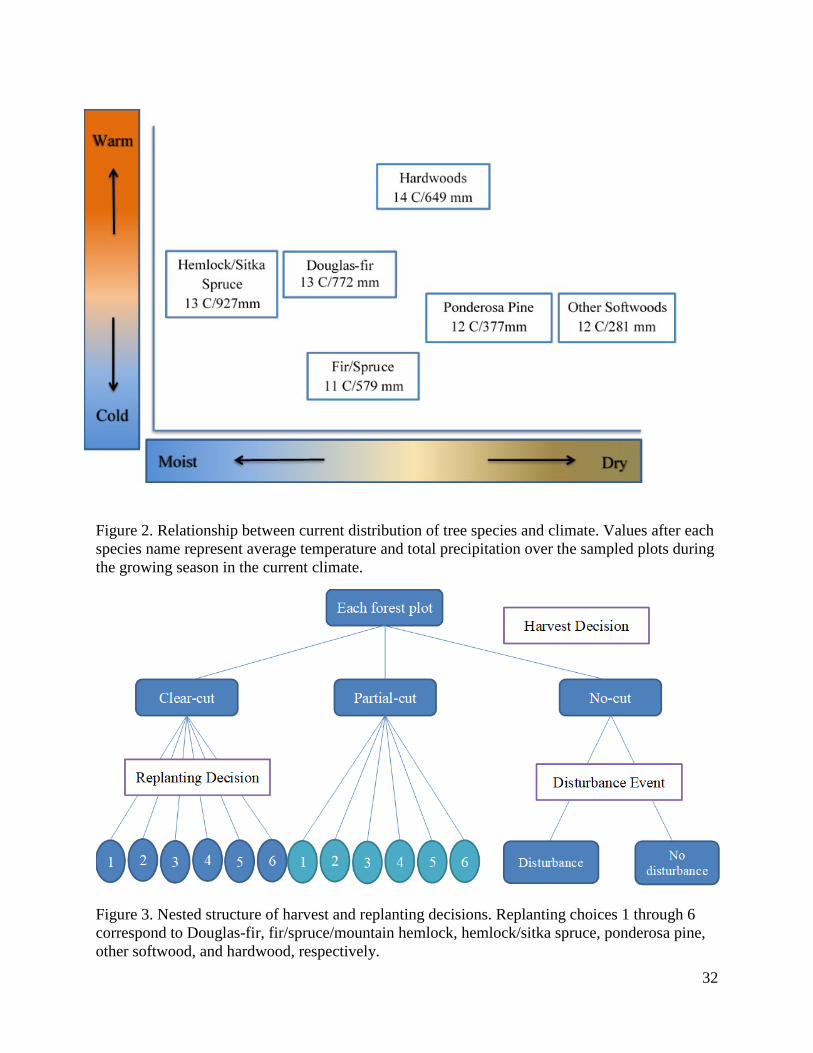
32

Figure 2. Relationship between current distribution of tree species and climate. Values after each species name represent average temperature and total precipitation over the sampled plots during the growing season in the current climate.

Figure 3. Nested structure of harvest and replanting decisions. Replanting choices 1 through 6 correspond to Douglas-fir, fir/spruce/mountain hemlock, hemlock/sitka spruce, ponderosa pine, other softwood, and hardwood, respectively.

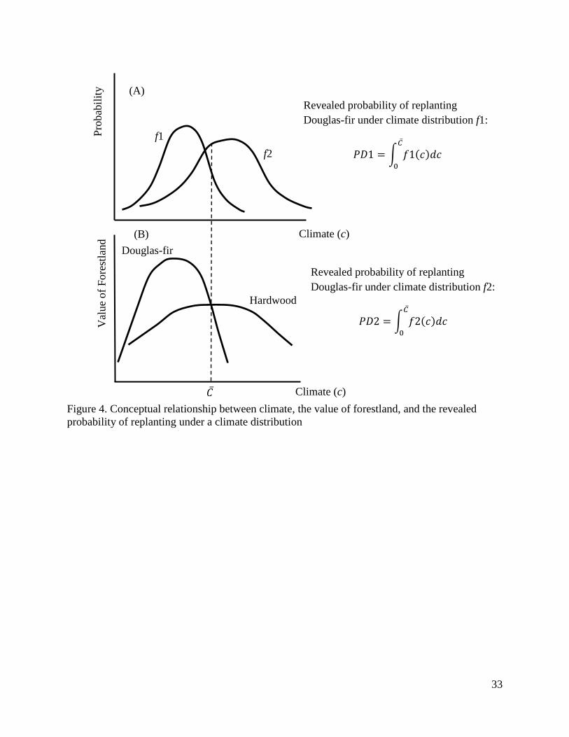
33

Figure 4. Conceptual relationship between climate, the value of forestland, and the revealed probability of replanting under a climate distribution

Prob

abili

ty

Val

ue o

f For

estla

nd

f1 f2

Climate (c)

Climate (c)

Douglas-fir

Hardwood

𝐶𝐶̅

𝑃𝑃𝑃𝑃1 = � 𝑓𝑓1(𝑐𝑐)𝑑𝑑𝑐𝑐𝐶𝐶̅

0

Revealed probability of replanting Douglas-fir under climate distribution f1:

𝑃𝑃𝑃𝑃2 = � 𝑓𝑓2(𝑐𝑐)𝑑𝑑𝑐𝑐𝐶𝐶̅

0

Revealed probability of replanting Douglas-fir under climate distribution f2:

(A)

(B)

34

Figure 5. Non-federal FIA forest plots on U.S. west coast. “Much warmer” and “much drier” indicate 4 C° or more increase in temperature and larger than 50 mm precipitation decrease, respectively.

5.a Current distribution of forest types

5.b Projected climate change

35

Figure 6. Partial effects of rent increase on replanting probabilities (top) and average plant viability scores (bottom). Dashed lines in 6.c and 6.d indicate range where species has little chance to be biophysically viable. Below the dashed lines the species has almost no chance to be viable.

6.a Partial effects of $10/acre rent increase on replanting Douglas-fir

-2%

-1%

0%

1%

2%

3%

4%Av

erag

e ch

ange

in re

plan

ting

prob

abili

ty

Climate

CA

Western OR

Western WA

Current 2030 2050 2070 2090

6.b Partial effects of $10/acre rent increase on replanting hardwood

0%

1%

2%

3%

4%

5%

6%

Aver

age

chan

ge in

repl

antin

g pr

obab

ility

Climate

p g

CA

Western OR

Western WA

Current 2030 2050 2070 2090

6.c Average Douglas-fir plant viability score (from Crookston et al. 2010)

6.d Average hardwood plant viability score (from Crookston et al. 2010)

36

Figure 7. Time path of each forest type's total landscape share under baseline scenario with no climate change (left), climate change only scenario (middle), and climate change & carbon pricing scenario (right). DF: Douglas-fir, FIR: fir/spruce, HEM: hemlock/sitka spruce, PP: ponderosa pine, OS: other softwood, and HW: hardwood.

37

Figure 8. Time path of each forest type's total replanting share under climate change only scenario (left) and carbon pricing scenario (right). The kinks in the chart are due to the change in the replanting choice set that is assigned to each plot. The choice set is based on the plant viability scores that reflects the likelihood that the climate at a given location would be suitable for each species.

38

Figure 9. Effects of climate change on landscape (left), harvested land only in 2090 (middle) and combined effects of climate change and carbon pricing on landscape (right) for Douglas-fir (top) and hardwood (bottom)

39

Table 1. Discrete effect of a 90-year climate and carbon price path on the probability of extensive margin adaption by switching from forest type and switching to forest type (western Oregon and western Washington as an example)

Region Initial forest type (switching from)

Effect of climate change

Effect of carbon price

Final forest type (switching to)

Effect of climate change

Effect of carbon price

West Oregon Douglas-fir 10.6% 6.9% Douglas-fir -5.5% -2.0%

Fir/Spruce -6.7% -2.1% Fir/Spruce 2.5% 0.4%

Hemlock/Sitka -3.6% 0.2% Hemlock/Sitka -3.8% -0.3%

Ponderosa Pine -8.8% 2.4% Ponderosa Pine 1.3% 0.7%

Other softwood -11.4% 0.2% Other softwood 0.6% -0.1%

Hardwood -16.5% -4.3% Hardwood 6.8% 4.6%

West Washington Douglas-fir 1.9% 4.2% Douglas-fir -5.6% -2.1%

Fir/Spruce -10.2% -1.0% Fir/Spruce 0.3% -0.2%

Hemlock/Sitka -2.7% 1.2% Hemlock/Sitka -4.1% -0.9%

Ponderosa Pine NA NA Ponderosa Pine 0.0% 0.0%

Other softwood -11.7% -0.3% Other softwood 1.6% 1.3%

Hardwood -15.1% -3.8% Hardwood 3.9% 3.2%