ARTICLE IN PRESS

Contents lists available at ScienceDirect

Journal of Financial Economics

Journal of Financial Economics 92 (2009) 223–237

0304-40

doi:10.1

$ We

individu

underst

Sialm, a

seminar

discussa

the disc

Montan

versity,

Technol

sity, Pu

Univers

Univers

Wiscon

support

Urbana-

and not� Cor

E-m

journal homepage: www.elsevier.com/locate/jfec

Individual investor mutual fund flows$

Zoran Ivkovic a,�, Scott Weisbenner a,b

a Michigan State University, East Lansing, MI 48824, USAb National Bureau of Economic Research, Cambridge, MA 02138, USA

a r t i c l e i n f o

Article history:

Received 18 May 2006

Received in revised form

16 April 2008

Accepted 12 May 2008Available online 22 January 2009

JEL classifications:

G11

C41

D14

H20

Keywords:

Mutual fund flows

Individual investor portfolio choice

Tax-motivated trading

5X/$ - see front matter & 2009 Elsevier B.V.

016/j.jfineco.2008.05.003

thank an anonymous discount broker for

al investors’ trades and Terry Odean for his he

anding the data set. Special thanks go to Josh

nd Jay Wang for many insightful suggestio

participants at the 2005 FEA Meetings at U

nt Jason Karceski), the 2006 EFA Meetings in

ussant Daniel Bergstresser), the 2007 WFA M

a (especially the discussant Sunil Wahal),

Florida State University, Hong Kong Univers

ogy, Michigan State University, Nanyang Tec

rdue University, Queens University, Singa

ity, the University of Illinois, the Universi

ity of Munster, the University of Texas, and

sin for useful comments. Both authors acknow

from the College Research Board at the Univ

Champaign. The views expressed herein are t

necessarily those of the National Bureau of E

responding author.

ail address: ivkovich@bus.msu.edu (Z. Ivkovic

a b s t r a c t

This paper studies the relation between individuals’ mutual fund flows and fund

characteristics, establishing three key results. First, consistent with tax motivations,

individual investors are reluctant to sell mutual funds that have appreciated in value

and are willing to sell losing funds. Second, individuals pay attention to investment

costs as redemption decisions are sensitive to both expense ratios and loads. Third,

individuals’ fund-level inflows and outflows are sensitive to performance, but in

different ways. Inflows are related only to ‘‘relative’’ performance, suggesting that new

money chases the best performers in an objective. Outflows are related only to

‘‘absolute’’ fund performance, the relevant benchmark for taxes.

& 2009 Elsevier B.V. All rights reserved.

All rights reserved.

providing data on

lp in obtaining and

ua Pollet, Clemens

ns. We also thank

NC (especially the

Zurich (especially

eetings in Big Sky,

Arizona State Uni-

ity of Science and

hnological Univer-

pore Management

ty of Indiana, the

the University of

ledge the financial

ersity of Illinois at

hose of the authors

conomic Research.

).

1. Introduction

The mutual fund literature has long recognized thatinvestors respond to mutual fund performance and hasdocumented a robust, positive relation between net fundflows and past fund performance (e.g., Ippolito, 1992;Chevalier and Ellison, 1997; Sirri and Tufano, 1998). Netflows, however, are differences of two nearly equally largecomponents—new purchases (inflows) and redemptions(outflows)1—that might well follow different patterns,and aggregation into net flows may preclude the devel-opment of more detailed insights.

1 During the period from 1984 to 2002, redemptions were almost as

large as new purchases, accounting for 48.5% of the sum of dollar

amounts of new purchases and redemptions. This figure is based on

authors’ calculations from the data reported in the 2003 Mutual Fund

Factbook (Investment Company Institute, 2004).

ARTICLE IN PRESS

Z. Ivkovic, S. Weisbenner / Journal of Financial Economics 92 (2009) 223–237224

Although the existing studies largely rely upon netflows, as dictated by data availability,2 a conventionalwisdom developed that the net flow-performance relationstems from the strong performance-chasing exhibited bynew buys, with little or no contribution to the relationfrom the redemption side. That notion, however, is notgrounded in a direct inquiry into the patterns of inflowsand outflows, and it might well be that redemptions arerelated to past performance. Also, inflows and outflowsmight be related to other fund characteristics verydifferently.

This paper studies the relation between individualinvestors’ mutual fund flows and a range of fundcharacteristics (past performance, proxies associated withpotential future fund-driven tax liabilities, and investmentcosts). We use detailed brokerage data featuring invest-ments a large sample of individual investors made in theperiod from 1991 to 1996. We first study individuals’ fundshare redemption decisions in both taxable and tax-deferred settings, and then proceed to study individualinvestor fund-level inflows and outflows by aggregatingthe purchases and redemptions from the brokerage databy month and by mutual fund and thus decomposingindividuals’ fund-level net flows into inflows and outflows(as well as, in additional analyses, decomposing the latterinto outflows in taxable accounts and outflows in tax-deferred accounts).

Individual investors’ mutual fund share redemptiondecisions might be related to fund performance sincepurchase for several (perhaps countervailing) reasons. Forone, there is the tax motivation. In the U.S., capital gainsare taxed on a realization basis, which provides investorswith an incentive to hold on to mutual fund shares whosenet asset value per share (NAV) has appreciated sincepurchase (thus delaying the payment of taxes) andredeem mutual fund shares whose NAV has fallen invalue since purchase (thus using those losses to reducetaxes right away).

A belief in performance persistence could also lead toholding funds that have appreciated in value sincepurchase and selling those that have fallen since purchase.Both tax motivations and belief in performance persis-tence predict a negative relation between propensity to

2 The data collection of aggregate fund-level inflows and outflows,

available from the Securities and Exchange Commission (SEC) in

electronic form since the mid-1990s, is onerous and very few studies

have pursued it (e.g., Edelen, 1999; Bergstresser and Poterba, 2002;

O’Neal, 2004; Cashman, Deli, Nardari, and Villupuram, 2006), and then

only, with the exception of Cashman, Deli, Nardari, and Villupuram

(2006), for a relatively small number of funds. The only other data set

that features the possibility of effective separation of net flows into

inflows and outflows in the domain of U.S. mutual fund investments of

which we are aware, used in Johnson (2007), are transactions of

shareholders in one small, no-load mutual fund family. Although the

number of investors covered by that data set is substantial (well over

50,000), its limitation is a narrow representation of funds (up to ten

funds) and, thus, limited cross-sectional variation of their characteristics.

Finally, data on inflows and outflows are available for U.K. mutual fund

investors (Keswani and Stolin, 2008), although their use to date has been

limited to assessing whether ‘‘money is smart,’’ with separate con-

sideration of inflows and outflows.

sell and past fund performance, although tax considera-tions matter only in taxable accounts.

On the other hand, psychological considerations seemto play an important role in individuals’ trading decisions.For example, the disposition effect—the propensity tocash in gains and aversion to realize losses (Kahnemanand Tversky, 1979; Shefrin and Statman, 1985)—wouldlead to a pronounced positive relation between redemp-tion decisions and fund performance since purchase.Although the disposition effect appears to be a dominantdeterminant of individual investors’ decisions to sellcommon stock shares (e.g., Odean, 1998; Grinblatt andKeloharju, 2001), there is little research inquiring whethersuch findings carry over to mutual funds.

To disentangle these competing hypotheses, we focuson the change of fund NAV since purchase. Naturally, thatperformance measure, as important as it is for taxationpurposes and for psychological explanations, is unlikely tobe the only determinant of individuals’ redemptiondecisions. Tax-sensitive investors might focus not onlyon the direct tax consequences related to the change ofthe fund NAV since purchase, but also on fund character-istics that could provide information regarding future funddistribution policy (such as turnover, past distributionbehavior, and capital gains overhang), information rele-vant for taxable investors because the tax rate ondistributions received generally exceeds the tax rate oncapital gains realized in the future upon sale.

Individuals’ mutual fund share redemption decisions inboth their taxable and tax-deferred accounts might alsobe sensitive to investment costs. The literature to date hasnot focused on these sensitivities at the individual-investor level. Rather, as in Barber, Odean, and Zheng(2005), analyses focus on the effects that investment costssuch as expenses and loads might have on mutual fundnet flows. However, as with fund performance, usefulinsights may be gleaned by breaking net flows into theirtwo components. For example, expense ratios might haveonly a modest relation with net flows, yet could havestrong positive effects both on ‘‘new’’ money flowing intothe fund (e.g., high expenses could partly be used foradvertising to help attract new investors or could beinterpreted as a signal of quality of fund management orservices provided by the fund family) and ‘‘old’’ moneyleaving the fund (e.g., in response to the higher ongoingcosts of maintaining the investment).

We establish three key findings. First, in stark contrastwith individual investor behavior in regard to commonstocks (Odean, 1998; Grinblatt and Keloharju, 2001), thereis a negative relation between the likelihood of sale andpast mutual fund performance for mutual funds held intaxable accounts. That is, investors holding mutual fundsin taxable accounts are reluctant to sell funds thatappreciated in value and willing to sell funds that havefallen in price.

A comparison of trades in taxable and tax-deferredaccounts suggests that the negative relation can beexplained by tax-motivated trading (i.e., capital gainslock-in and tax-loss selling) because there is no statisti-cally significant relation between redemption probabilityand fund performance since purchase in tax-deferred

ARTICLE IN PRESS

Z. Ivkovic, S. Weisbenner / Journal of Financial Economics 92 (2009) 223–237 225

accounts. Thus, on net, psychological motivations appearto play much less of a role in the domain of individuals’mutual fund investments than they do in the domain ofinvestment in individual stocks.

In further support for tax-motivated trading, we findthat taxable investors’ redemption decisions are sensitiveto proxies for future distribution behavior of the fund. Intaxable accounts, the fund turnover ratio, the historicalshare of total fund returns distributed to the fund in-vestors over the preceding five years, and the fund capitalgains overhang—three proxies for future fund distributionbehavior—are all positively related to redemption prob-ability. By contrast, in tax-deferred accounts turnoverdoes not play a role in redemption decisions and therelation between redemption probability and past funddistribution policy is significantly weaker than it is intaxable accounts.3

Our second key result is that mutual fund investors aresensitive to both front-end loads (an ‘‘in-your-face’’ cost ofmutual fund investments) and expense ratios (a moresubtle, ongoing cost). The latter yields a finding thatdiffers from the conclusions reported in Barber, Odean,and Zheng (2005), though the differential could beattributed to the fact that we are looking into individuals’redemption decisions, whereas Barber, Odean, and Zheng(2005) focus on quarterly net fund flows.

Our third key result stems from aggregation ofindividual investors’ buys and sells into monthly mea-sures of fund-level inflows and outflows. Consistent withthe notion that new money chases the best performers,we find that inflows are related only to funds’ relativeperformance measures, that is, funds’ one-year perfor-mance relative to other funds pursuing the same objec-tive. On the other hand, as expected in light of thetransaction-level results, outflows are related only tofunds’ one-year ‘‘absolute’’ returns. The latter finding isconsistent with tax motivations, as it is the absolutechange in NAV that is relevant for taxable investors’ taxliability following a sale. Thus, both new money and oldmoney are sensitive to past fund performance, but in verydifferent ways.

Finally, we also consider the role that the investmentcosts play in the context of fund-level flows. The moststriking finding is that individuals’ fund-level inflows andoutflows are each positively related to expense ratios—

whereas higher expenses may attract more new moneythrough advertising or a perception that higher expensesreflect better managerial talent or fund family services,they also prompt old money to leave the fund sooner thanit otherwise would. We also find sensitivity to loads,particularly for outflows.

These rich characterizations are obscured when in-flows and outflows are combined and only net flows arestudied. Our results stress that the absence of a relationbetween net flows and a fund characteristic does notimply that the characteristic is unimportant for all

3 Somewhat curiously, the redemption decision is sensitive to

capital gains overhang not only in taxable accounts, but also in tax-

deferred accounts (where tax motivations are absent).

investors. Indeed, given that new or potential investorsin the fund and the incumbent investors may havedifferent considerations, disentangling net flows into itscomponents is important. The most glaring examples areconsiderations of absolute performance, expenses, andloads, all of which are of substantial importance to theincumbent investors considering a sale of their fundshares.

The remainder of this paper is organized as follows. InSection 2 we review the data and present some summarystatistics. Section 3 presents the results of analyses thatrelate probability of sale of individuals’ mutual fundinvestments with a range of fund characteristics, includ-ing past performance, determinants of future potential taxliabilities, and investment costs. In Section 4 we aggregateinvestors’ buys and sells of mutual funds into monthlymeasures of inflows and outflows, and analyze thedeterminants of those flows. Section 5 concludes.

2. Data description and summary statistics

2.1. Data description

Our primary data set, trades that 78,000 householdsmade in the period from January of 1991 to November of1996, comes from a large discount broker. Mutual fundsare the second most frequently used investment vehicle inthe data set, accounting for 18% of the overall value of allthe trades investors in the sample made over the six-yearperiod. They are second only to common stocks (whichaccount for around two-thirds of the overall value of theinvestments in the sample). A number of households havemultiple accounts (such as one taxable and one tax-deferred account); the median number of accounts perhousehold is two.

Around 32,300 households made at least one mutualfund purchase during the sample period either in taxableor tax-deferred accounts (IRAs and Keogh plans; retire-ment plan accounts provided through employment suchas 401(k)-type plans are not part of the data set). For adetailed description of the brokerage data set see Barberand Odean (2000).

Mutual fund returns, rankings, and fund characteristicscome from the Center for Research in Security Prices(CRSP) Open-End Mutual Fund Database and Morningstar.We extract the relevant information regarding samplefunds’ investment objectives from the CRSP mutual funddatabase fields ‘‘Objective’’ and ‘‘ICDI Objective.’’ Ourbrokerage sample contains transactions covering morethan 1,100 different mutual funds across 200 differentmutual fund families that span more than 40 differentinvestment objective categories. We will control forheterogeneity both on the individual-investor level, aswell as the mutual-fund-type level, by allowing saledecisions to vary by the mutual fund family, by theobjective of the mutual fund, by whether the fund isactively or passively managed (i.e., is it an index fund), aswell as by whether the transaction is in a taxable or a tax-deferred account.

ARTICLE IN PRESS

Table 1Summary statistics of mutual fund purchases and sales.

The sample consists of 32,259 households that made at least one mutual fund purchase through a large discount broker during the period from January

1991 to November 1996. This table presents basic summary statistics (median dollar amount of purchase and number of purchases are reported in

parentheses).

Number of

purchases

Average $ amount of

purchases (Median)

Average # of purchases per

household, conditional on purchase

in that type of account (Median)

Percentage of purchases sold

during the sample period

All accounts 325,185 8,394 10.1 34

(3,000) (4.0)

Taxable accounts 180,564 9,376 8.5 33

(3,000) (3.0)

Tax-deferred accounts 144,621 7,169 7.2 35

(3,000) (3.0)

Z. Ivkovic, S. Weisbenner / Journal of Financial Economics 92 (2009) 223–237226

Consistent with Ivkovic, Poterba, and Weisbenner(2005), we include in our sample all mutual fund sharepurchases (and follow the purchase to see whether thereis a subsequent sale), with one exception: in the instancesin which multiple buys are followed by a sale, it is notpossible to match unambiguously which purchased fundshares actually have been sold without making assump-tions such as FIFO (first share bought, first share sold) orLIFO (last share bought, first share sold), which by itselfcould drive the results.4 The exclusion of multiple buyspreceding an ambiguous sale reduces the number ofpurchases in the sample by around 20%.

Also, in the instances in which multiple sales follow asingle purchase, only the first sale is admitted into thesample, which means that our analyses may slightlyunderstate the actual holding periods for these mutualfund investments. However, that bias is negligible becausethe vast majority of mutual fund sales in the sample (89%)are complete liquidations of the respective positions.

2.2. Summary statistics

Table 1 presents summary statistics on mutual fundpurchases and subsequent sales in the sample. Applyingthe criteria outlined above results in 325,185 buys madeover the sample period, representing 32,259 householdsthat had at least one mutual fund purchase during thesample period. The numbers of mutual fund purchases intaxable accounts and tax-deferred accounts, as well asmedian dollar amounts of those purchases, are verysimilar. Approximately one-third of the purchases werefollowed by a sale during the sample period.

2.3. Graphical summary of hazard rates and past NAV

change

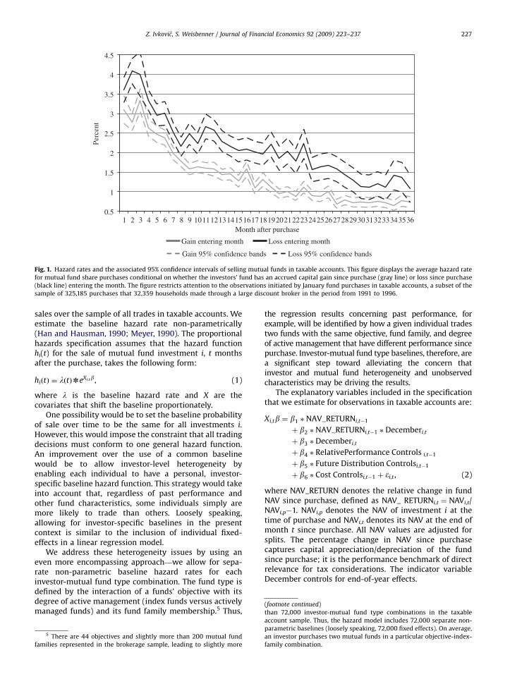
Fig. 1 presents monthly hazard rates (i.e., the likelihoodof sale during a given month after purchase conditional on

4 For example, in an upward market (as generally was the case

during much of the sample period) fund shares purchased first in a string

of purchases would have a larger appreciation since purchase than the

last share in a string of purchases. Therefore, assuming FIFO would

induce a positive relation between redemption probability and past fund

performance.

having not sold up to that month) of individuals’ sales ofmutual fund shares held in their taxable accounts. Thetwo solid lines depict hazard rates conditional upon thefund NAV having increased since purchase (gray solid line)and hazard rates conditional upon the fund NAV havingdecreased since purchase (black solid line) for each of thefirst 36 months following the purchase. For the purposesof this figure we restrict our attention to all mutual fundpurchases in taxable accounts in January. This strategyallows for identification of end-of-year effects and otherpatterns potentially related to the calendar month. Weobtain the confidence intervals presented in Fig. 1 bycalculating standard errors that allow for heteroskedasti-city as well as correlation across observations associatedwith the same individual.

The figure identifies two very pronounced empiricalfacts that differentiate sales of mutual fund shares fromsales of common stocks (Odean, 1998; Grinblatt andKeloharju, 2001). First, in stark contrast with commonstock investments, hazard rates conditional upon lossesexceed those conditional upon gains. Thus, on net,psychological motivations such as the disposition effectappear to play much less of a role in the domain ofindividuals’ mutual fund investments than they do in thedomain of investment in individual stocks.

Second, hazard rates of selling mutual fund shares intaxable accounts, although declining like the hazard ratesfor common stocks, are significantly smaller than thosefor stocks. For example, in the first few months theunconditional hazard rates of selling mutual fund sharesare around 3–4%, whereas the comparable hazard rates ofselling common stocks start as high as 15% after onemonth, 10% after two months, and 8% after three months(Ivkovic, Poterba, and Weisbenner, 2005). This discre-pancy suggests that high-frequency traders are not nearlyas present in the arena of mutual fund investments.

3. Analysis of redemption decisions

We proceed with analyses of the relation betweenpropensity to sell fund shares and a range of fundcharacteristics, contrasting redemption behavior in tax-able and tax-deferred settings. We begin by estimating aCox proportional hazards model of mutual fund share

ARTICLE IN PRESS

0.5

1

1.5

2

2.5

3

3.5

4

4.5

1Month after purchase

Perc

ent

Gain entering month Loss entering month

Gain 95% confidence bands Loss 95% confidence bands

2 3 4 5 6 7 8 9 101112131415161718192021222324252627282930313233343536

Fig. 1. Hazard rates and the associated 95% confidence intervals of selling mutual funds in taxable accounts. This figure displays the average hazard rate

for mutual fund share purchases conditional on whether the investors’ fund has an accrued capital gain since purchase (gray line) or loss since purchase

(black line) entering the month. The figure restricts attention to the observations initiated by January fund purchases in taxable accounts, a subset of the

sample of 325,185 purchases that 32,359 households made through a large discount broker in the period from 1991 to 1996.

(footnote continued)

than 72,000 investor-mutual fund type combinations in the taxable

Z. Ivkovic, S. Weisbenner / Journal of Financial Economics 92 (2009) 223–237 227

sales over the sample of all trades in taxable accounts. Weestimate the baseline hazard rate non-parametrically(Han and Hausman, 1990; Meyer, 1990). The proportionalhazards specification assumes that the hazard functionhi(t) for the sale of mutual fund investment i, t monthsafter the purchase, takes the following form:

hiðtÞ ¼ lðtÞn eXi;tb, (1)

where l is the baseline hazard rate and X are thecovariates that shift the baseline proportionately.

One possibility would be to set the baseline probabilityof sale over time to be the same for all investments i.However, this would impose the constraint that all tradingdecisions must conform to one general hazard function.An improvement over the use of a common baselinewould be to allow investor-level heterogeneity byenabling each individual to have a personal, investor-specific baseline hazard function. This strategy would takeinto account that, regardless of past performance andother fund characteristics, some individuals simply aremore likely to trade than others. Loosely speaking,allowing for investor-specific baselines in the presentcontext is similar to the inclusion of individual fixed-effects in a linear regression model.

We address these heterogeneity issues by using aneven more encompassing approach—we allow for sepa-rate non-parametric baseline hazard rates for eachinvestor-mutual fund type combination. The fund type isdefined by the interaction of a funds’ objective with itsdegree of active management (index funds versus activelymanaged funds) and its fund family membership.5 Thus,

5 There are 44 objectives and slightly more than 200 mutual fund

families represented in the brokerage sample, leading to slightly more

the regression results concerning past performance, forexample, will be identified by how a given individual tradestwo funds with the same objective, fund family, and degreeof active management that have different performance sincepurchase. Investor-mutual fund type baselines, therefore, area significant step toward alleviating the concern thatinvestor and mutual fund heterogeneity and unobservedcharacteristics may be driving the results.

The explanatory variables included in the specificationthat we estimate for observations in taxable accounts are:

Xi;tb ¼ b1 �NAV_RETURNi;t�1

þ b2 �NAV_RETURNi;t�1 � Decemberi;t

þ b3 � Decemberi;t

þ b4 � RelativePerformance Controls i;t�1

þ b5 � Future Distribution Controlsi;t�1

þ b6 � Cost Controlsi;t�1 þ �i;t , (2)

where NAV_RETURN denotes the relative change in fundNAV since purchase, defined as NAV_ RETURNi,t ¼ NAVi,t/NAVi,p�1. NAVi,p denotes the NAV of investment i at thetime of purchase and NAVi,t denotes its NAV at the end ofmonth t since purchase. All NAV values are adjusted forsplits. The percentage change in NAV since purchasecaptures capital appreciation/depreciation of the fundsince purchase; it is the performance benchmark of directrelevance for tax considerations. The indicator variableDecember controls for end-of-year effects.

account sample. Thus, the hazard model includes 72,000 separate non-

parametric baselines (loosely speaking, 72,000 fixed effects). On average,

an investor purchases two mutual funds in a particular objective-index-

family combination.

ARTICLE IN PRESS

Z. Ivkovic, S. Weisbenner / Journal of Financial Economics 92 (2009) 223–237228

Relative Performance Controls include the percentileranking of one-year total returns within the fund’s invest-ment objective and the fund’s Morningstar 5-star rating.Future Distribution Controls are predictors of future dis-tribution policy (turnover, past fund distribution policy, andfund overhang) that capture indirect tax motivations. Finally,Cost Controls capture investment costs (expense ratios,front-end loads, and back-end loads).

Investors covered by the data set can have both taxableand tax-deferred accounts (i.e., IRA and Keough plans;investments in 401(k) plans are not part of the brokeragesample). Under the assumption that the disposition effectand the belief in fund performance persistence do notdiffer across investments in taxable and tax-deferredaccounts, comparing the propensities to sell acrossmutual fund holdings in the two types of accountsprovides a direct way of identifying the impact of taxationbecause tax considerations should not affect tradingdecisions in tax-deferred accounts.6

Accordingly, we also estimate regressions over the fullsample of taxable and tax-deferred accounts. The modelallows for separate non-parametric baseline hazard ratesfor each investor-mutual fund type combination, intro-duced separately for an investor’s holdings in taxable andtax-deferred accounts. We introduce an indicator variableTAXi that denotes whether the mutual fund investment i

is held in a taxable account and interact TAXi with all ofthe preceding variables:

Xi;ta ¼ a1 � NAV_RETURNi;t�1

þ a2 � NAV_RETURNi;t�1 � Decemberi;t

þ a3 � Decemberi;t

þ Other Controlsi;t�1 � a4

þ a5 � NAV_RETURNi;t�1 � TAXi

þ a6 � NAV_RETURNi;t�1 � Decemberi;t � TAXi

þ a7 � Decemberi;t � TAXi

þ Other Controlsi;t�1 � a8 � TAXi þ �i;t . (3)

In this regression, estimated over the pooled sample ofmutual fund investments in taxable and tax-deferredaccounts, the coefficient a1 represents the sensitivity ofthe sale decision to NAV performance since purchase intax-deferred accounts, the coefficient a5 represents thedifferential behavior in taxable accounts relative to tax-deferred accounts, and a1+a5 equals the sensitivity of thesale decision to NAV performance since purchase intaxable accounts (which corresponds to the coefficientb1 from Eq. (2)).

We present the results of the regressions based on Eqs.(2) and (3) in Table 2.7 For presentational convenience, we

6 This strategy is used in Ivkovic, Poterba, and Weisbenner (2005) to

study individual investors’ tax-motivated trading of common stocks. A

stronger disposition effect in taxable accounts than in tax-deferred

accounts would bias against, whereas a stronger belief in fund

performance persistence in taxable accounts would bias in favor of,

finding evidence of tax-motivated trading.7 A potential selection issue might arise because the sample consists

of mutual fund trades placed by households that need not have both

taxable and tax-deferred accounts. To address this concern, we run these

analyses on a more restrictive sample of all mutual fund trades placed by

the more than 17,000 households that have both types of accounts and

group our discussion of covariates into those related tofund performance since purchase, relative performancerankings, indirect tax motivations, and investment costs(Sections 3.1–3.4, respectively).

3.1. Motivations for negative relation between sale

propensity and performance since purchase

The negative relation between the likelihood of saleand past fund performance shown in Fig. 1 is consistentwith tax-related motivations. In taxable environments(but not tax-deferred ones), a realization-based capitalgains tax system provides incentives to sell investmentsthat have fallen in price (‘‘tax-loss selling’’) and keepinvestments that have risen in price (the ‘‘lock-in’’ effect).

Another plausible explanation for the negative relationbetween the propensity to sell and performance sincepurchase is investors’ potential belief in fund performancepersistence. If investors believe that funds’ past fundperformance is indicative of their future performance, onthe margin, they would be more likely to sell past losersand hold on to past winners. This should be equally true intaxable and tax-deferred (i.e., IRA and Keough) accounts.

In this section, we employ a hazard-model frameworkin a setting with numerous controls for fund character-istics to perform a detailed analysis of the negativerelation found in the parsimonious estimates displayedin Fig. 1. We seek to differentiate between the alternativehypotheses for the negative relation by considering theresults in taxable and tax-deferred settings. Finally, wealso analyze the effects of other fund characteristics.

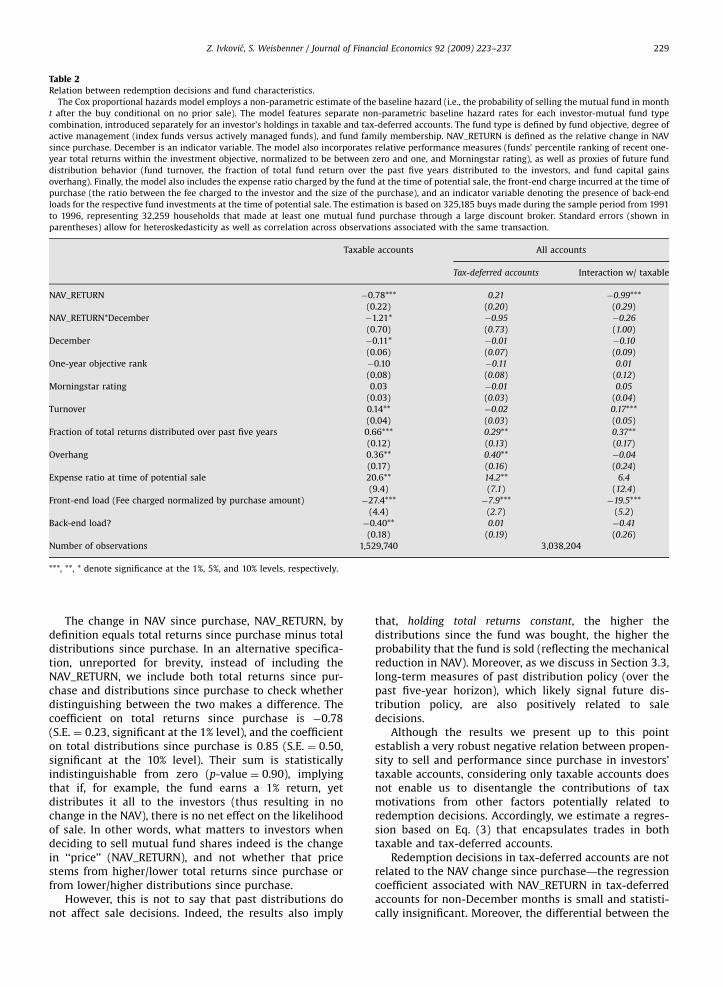
The results of estimating the model from Eq. (2) acrossall taxable mutual fund investments are presented in thefirst column of Table 2. Consistent with Fig. 1, evidence insupport of a negative relation is very pronouncedthroughout the calendar year. The coefficient for NAV_RETURN is �0.78, suggesting that, in months other thanDecember, a 25% increase in NAV since purchase isassociated with an 18% decrease in probability of sale(calculated as e�0.78

*0.25�1 ¼ �0.18). The coefficient for

NAV_RETURN*December is large and negative (�1.21),indicating that tax-motivated trading is the most intenseat the end of the year.

To gauge the economic significance of the redemption-performance relation, we perform a simple, back-of-the-envelope calculation. According to the InvestmentCompany Institute (2004), over the past two decades theratio of aggregate sales to aggregate assets across allequity mutual funds is roughly 30% on an annual basis.The estimate that a 25% increase in NAV since purchasereduces the probability of sale by 18% suggests that, incase of such a NAV increase, total assets under manage-ment would increase—very loosely—by about 5%(30*0.18) on an annual basis through the decreasedredemptions, which constitutes a sizeable fraction of totalassets under management.

(footnote continued)

find that the results are very similar to those reported in Table 2, a

finding that is not surprising given all of the controls for heterogeneity of

investors already included in the model.

ARTICLE IN PRESS

Table 2Relation between redemption decisions and fund characteristics.

The Cox proportional hazards model employs a non-parametric estimate of the baseline hazard (i.e., the probability of selling the mutual fund in month

t after the buy conditional on no prior sale). The model features separate non-parametric baseline hazard rates for each investor-mutual fund type

combination, introduced separately for an investor’s holdings in taxable and tax-deferred accounts. The fund type is defined by fund objective, degree of

active management (index funds versus actively managed funds), and fund family membership. NAV_RETURN is defined as the relative change in NAV

since purchase. December is an indicator variable. The model also incorporates relative performance measures (funds’ percentile ranking of recent one-

year total returns within the investment objective, normalized to be between zero and one, and Morningstar rating), as well as proxies of future fund

distribution behavior (fund turnover, the fraction of total fund return over the past five years distributed to the investors, and fund capital gains

overhang). Finally, the model also includes the expense ratio charged by the fund at the time of potential sale, the front-end charge incurred at the time of

purchase (the ratio between the fee charged to the investor and the size of the purchase), and an indicator variable denoting the presence of back-end

loads for the respective fund investments at the time of potential sale. The estimation is based on 325,185 buys made during the sample period from 1991

to 1996, representing 32,259 households that made at least one mutual fund purchase through a large discount broker. Standard errors (shown in

parentheses) allow for heteroskedasticity as well as correlation across observations associated with the same transaction.

Taxable accounts All accounts

Tax-deferred accounts Interaction w/ taxable

NAV_RETURN �0.78*** 0.21 �0.99***

(0.22) (0.20) (0.29)

NAV_RETURN*December �1.21* �0.95 �0.26

(0.70) (0.73) (1.00)

December �0.11* �0.01 �0.10

(0.06) (0.07) (0.09)

One-year objective rank �0.10 �0.11 0.01

(0.08) (0.08) (0.12)

Morningstar rating 0.03 �0.01 0.05

(0.03) (0.03) (0.04)

Turnover 0.14** �0.02 0.17***

(0.04) (0.03) (0.05)

Fraction of total returns distributed over past five years 0.66*** 0.29** 0.37**

(0.12) (0.13) (0.17)

Overhang 0.36** 0.40** �0.04

(0.17) (0.16) (0.24)

Expense ratio at time of potential sale 20.6** 14.2** 6.4

(9.4) (7.1) (12.4)

Front-end load (Fee charged normalized by purchase amount) �27.4*** �7.9*** �19.5***

(4.4) (2.7) (5.2)

Back-end load? �0.40** 0.01 �0.41

(0.18) (0.19) (0.26)

Number of observations 1,529,740 3,038,204

***, **, * denote significance at the 1%, 5%, and 10% levels, respectively.

Z. Ivkovic, S. Weisbenner / Journal of Financial Economics 92 (2009) 223–237 229

The change in NAV since purchase, NAV_RETURN, bydefinition equals total returns since purchase minus totaldistributions since purchase. In an alternative specifica-tion, unreported for brevity, instead of including theNAV_RETURN, we include both total returns since pur-chase and distributions since purchase to check whetherdistinguishing between the two makes a difference. Thecoefficient on total returns since purchase is �0.78(S.E. ¼ 0.23, significant at the 1% level), and the coefficienton total distributions since purchase is 0.85 (S.E. ¼ 0.50,significant at the 10% level). Their sum is statisticallyindistinguishable from zero (p-value ¼ 0.90), implyingthat if, for example, the fund earns a 1% return, yetdistributes it all to the investors (thus resulting in nochange in the NAV), there is no net effect on the likelihoodof sale. In other words, what matters to investors whendeciding to sell mutual fund shares indeed is the changein ‘‘price’’ (NAV_RETURN), and not whether that pricestems from higher/lower total returns since purchase orfrom lower/higher distributions since purchase.

However, this is not to say that past distributions donot affect sale decisions. Indeed, the results also imply

that, holding total returns constant, the higher thedistributions since the fund was bought, the higher theprobability that the fund is sold (reflecting the mechanicalreduction in NAV). Moreover, as we discuss in Section 3.3,long-term measures of past distribution policy (over thepast five-year horizon), which likely signal future dis-tribution policy, are also positively related to saledecisions.

Although the results we present up to this pointestablish a very robust negative relation between propen-sity to sell and performance since purchase in investors’taxable accounts, considering only taxable accounts doesnot enable us to disentangle the contributions of taxmotivations from other factors potentially related toredemption decisions. Accordingly, we estimate a regres-sion based on Eq. (3) that encapsulates trades in bothtaxable and tax-deferred accounts.

Redemption decisions in tax-deferred accounts are notrelated to the NAV change since purchase—the regressioncoefficient associated with NAV_RETURN in tax-deferredaccounts for non-December months is small and statisti-cally insignificant. Moreover, the differential between the

ARTICLE IN PRESS

8 It is defined as the ratio (1+TOTAL_RETURNt�61, t�1�NAV_

RETURNt�61, t�1)/(1+TOTAL_RETURNt�61,t�1).

Z. Ivkovic, S. Weisbenner / Journal of Financial Economics 92 (2009) 223–237230

coefficients associated with the two types of accounts islarge and highly statistically significant. This suggests thatthe negative relation between the likelihood of redemp-tion and past performance in taxable accounts is ex-plained by tax-motivated trading. The lack of a relation intax-deferred accounts suggests that, to whatever extentinvestor belief in fund performance persistence and thedisposition effect are present in the domain of mutualfund investments, their net effect is such that they entirelyoffset each other (the negative relation resulting frombelief in fund performance persistence cancels out thepositive relation resulting from the disposition effect).

3.2. Effects of relative performance measures

Aside from the absolute performance of a fund sincepurchase (which is germane for tax purposes in case ofredemption), also relevant for an investor may be theperformance of that fund relative to funds pursuing thesame investment objective. Indeed, investors are suppliedroutinely with the information regarding fund perfor-mance over certain investment horizons, as well as withratings based on such performance, and may incorporatethis information into their decision-making. The perfor-mance measures that we consider are the percentileranking of recent one-year total returns within theinvestment objective (normalized to be between zeroand one) and 5-star Morningstar rating, both of which arecommonly used in the literature (see, e.g., Chevalier andEllison, 1997; Sirri and Tufano, 1998; Bergstresser andPoterba, 2002).

Relative performance measures have no effects on thepropensity to sell in either taxable or tax-deferredaccounts (after all, absolute and not relative benchmarksare relevant for tax purposes). Thus, the sensitivity of net

fund flows to relative performance rankings (e.g., Ippolito,1992; Chevalier and Ellison, 1997; Sirri and Tufano, 1998)seems to be driven by inflows, rather than by redemptionbehavior (which we confirm in aggregated-flow analysespresented in Section 4).

3.3. Indirect tax considerations

Tax-sensitive investors might focus not only on thedirect tax consequences related to the change of the fundNAV since purchase, but also on fund characteristics thatcould provide information regarding future fund distribu-tion policy because the tax rate on distributions receivedgenerally exceeds the tax rate on capital gains realized inthe future upon sale. Having discussed the tax implica-tions of NAV changes since purchase in Section 3.1, in thissection we discuss the somewhat more subtle taximplications that may stem from fund managers’ futuredistribution behavior.

In our empirical analyses we employ three proxiesrelated to future distribution behavior. First, our specifica-tions include fund turnover. According to Frazzini (2006),mutual fund managers exhibit behavior consistent withthe disposition effect, that is, they are likely to sell thewinners in their portfolios. Thus, turnover should be

positively related to future distributions because therewill be capital gains realized by such selling of the winnersfrom the fund portfolio. Accordingly, on the margin, thereshould be a positive relation between the propensity to selltaxable mutual fund investments (and thereby avoid futuredistributions) and fund turnover.

Second, fund distribution policy might be highlypersistent, in which case past distribution behavior mightbe indicative of future distributions. Thus, we constructour second proxy to reflect the fraction of total returns inthe form of distributions over the past five years (monthst�61 through t�1) preceding the month of potentialsale t.8 Finally, the fund’s capital gains overhang repre-sents potential capital gains realizations that might berealized, depending on the fund manager’s strategy andliquidity needs, in which case they would lead to futuredistributions and thus trigger a tax liability for the currenttaxable fund investments. Therefore, the relation betweenthe propensity to sell taxable mutual fund investmentsand fund capital gains overhang should be positive.

Our results further reinforce the importance of tax-motivated behavior. In taxable accounts, the fund turn-over ratio, the historical share of total fund returnsdistributed to the fund investors over the preceding fiveyears, and the fund capital gains overhang are allpositively related to the sale probability. By contrast,turnover does not play a role in sale decisions in tax-deferred accounts. Moreover, the relation between saleprobability and historical distributions is also weaker intax-deferred accounts. Somewhat curiously, the sensitiv-ity of sale decisions to overhang is virtually identicalacross the two types of accounts. On net, the evidencesuggests that direct (has the fund price gone up or downsince purchase?) and more subtle, indirect (is the fundlikely to pay out high future distributions?) tax motiva-tions both play important roles in individuals’ saledecisions.

Another way of interpreting these results is that bothpast and future distributions matter to investors. Bothincrease the probability that old money leaves the fund.Past distributions increase the probability of sale bymechanically reducing the NAV_RETURN, whereas proxiesfor future distributions increase the probability of salebecause of likely higher associated future tax liabilities(with both of these effects much stronger in taxableaccounts).

3.4. Effects of costs of mutual fund investment

A priori, one might expect no relation between thepropensity to sell and front-end charges (once fund sharesare purchased, front-end charges are a sunk cost). On theother hand, expense ratios (costs that investors incur on aregular basis for as long as they hold the fund shares) andback-end loads are costs still ahead for mutual fundinvestors and they might alter the probability ofsale. Higher expense ratios imply a stream of higher

ARTICLE IN PRESS

9 The results concerning loads are very robust. In addition to the

specifications reported in Table 2, we explored alternative ways of

capturing sensitivity to loads. First, we ran a specification in which both

front-end loads and back-end loads are captured with indicator

variables; we find investor sensitivity to both types of loads in this

regression as well. Second, we ran a specification in which, in addition to

front-end loads and back-end loads, we introduced an indicator variable

that captures the absence of loads altogether (that is, it captures no-load

funds). This additional no-load indicator variable was insignificant in its

own right; moreover, it did not alter any of the results presented in

Table 2 (the coefficients on the original load variables were essentially

unchanged).

Z. Ivkovic, S. Weisbenner / Journal of Financial Economics 92 (2009) 223–237 231

investment costs for as long as the investor owns the fundand thus, ceteris paribus, could be related positively withthe probability of sale. By contrast, back-end loads canreadily be conceived as deterrents to sale.

Barber, Odean, and Zheng (2005) consider the impactof front-end loads and expense ratios on individualinvestors’ mutual fund investment decisions, but theylimit their attention to the relation between net fund flowsaggregated across a large number of individuals andlagged values of expense ratios and front-end loads, ratherthan on individuals’ decisions to sell the mutual fundshares once they had acquired them. Barber, Odean, andZheng (2005) report that net fund flows are sensitive toin-your-face costs such as front-end loads, yet are notsensitive to the more subtle, ongoing costs such asexpense ratios.

To explore the impact of investment costs, we considerexpense ratios charged by the funds at the time ofpotential sale, front-end charges that investors incurredat the time of purchase (expressed as the ratio betweenthe fee charged to the investor and the size of thepurchase), and an indicator variable denoting the pre-sence of back-end loads for the respective fund invest-ments at the time of potential sale.

First, the level of the expense ratio at the time ofpotential sale increases the likelihood that the investorwill sell the mutual fund (effects are very similar acrosstaxable and tax-deferred accounts). For example, com-pared to a fund with annual expenses of 50 basis points, afund with annual expenses of 100 basis points is 11% morelikely to be sold in taxable accounts ðe20:6n0:01=e20:6n0:005 �

1 ¼ 0:11Þ, suggesting that individual investors are sensi-tive to the ongoing, subtle costs of investments. Thissensitivity is economically significant. Resorting onceagain to the data provided by the Investment CompanyInstitute (2004) and performing another back-of-the-envelope calculation, such a 50-basis point increase inexpense ratios loosely translates into a 3% decline(30*0.11) of total assets under management on an annualbasis.

We also ran a specification in which we break thecurrent expense ratio into the expense ratio at the time ofpurchase and the change in the expense ratio sincepurchase. In unreported results, we find that both arepositively related to the propensity of sale and arestatistically significant, with the coefficient on the changein the expense ratio of 54.6 (S.E. ¼ 16.3) being signifi-cantly greater in magnitude than the coefficient for theexpense ratio at the time of purchase of 19.2 (S.E. ¼ 9.4).Thus, investors who originally purchased a high-expensefund are more likely to sell that fund at any point in thefuture than are investors who purchased a low-expensefund, with investors responding particularly strongly ifthere was a change in the expense ratio since they madethe purchase.

Second, investors appear to view front-end charges asan impediment to sale, potentially because they mis-perceive the front-end charge as a marginal rather than asunk cost. The effect is more pronounced in taxableaccounts, but both types of accounts feature a large andnegative coefficient on the front-end load variable,

suggesting that a front-end load of 5% reduces themonthly likelihood of sale by 75% in taxable accountsand 33% in tax-deferred accounts.

One might conjecture that this large effect simplyreflects investor heterogeneity—households that invest infunds with front-end loads tend to have longer holdingperiods. However, the specification controls for consider-able heterogeneity through investor-mutual fund typeeffects (non-parametric baselines). Thus, the correlationbetween front-end loads and sale decisions cannot simplybe attributed, for example, to buy-and-hold investorspurchasing funds with front-end loads. Rather, theregression results are identified by how a given individualtrades two funds with the same objective, fund family,and degree of active management that have differentfront-end loads.

As a result, the front-end load effect likely does notmerely reflect investor heterogeneity and may insteadreflect investors’ sunk cost fallacy (i.e., a confusion of sunkand marginal costs). Supporting this interpretation issurvey evidence we obtained for a separate, ongoingproject: nearly three-quarters of a random sample of 276mutual fund investors that own funds with front-endloads report the need to hold the fund long enough tojustify the front-end load; only one-quarter of thesurveyed investors report that, after the fund had beenpurchased, the front-end load does not affect how longthey hold on to the fund.

Finally, there is some evidence that investors aresensitive to back-end loads as well, but the resultsregarding the presence of a back-end load are not quiteas strong as those for the front-end load. Whereas thenegative and statistically significant coefficient for taxableaccounts (�0.40; S.E. ¼ 0.18) suggests that back-end loadsserve as a deterrent to sales, this does not carry over totax-deferred accounts, for which the coefficient is vir-tually zero (the difference between the coefficients acrosstaxable and tax-deferred coefficients, though, is notstatistically significant).9

4. Determinants of monthly fund inflows and outflows

The preceding section reveals a very rich characteriza-tion of determinants of individuals’ transaction-levelmutual fund sale decisions. It shows that relativeperformance is unimportant for redemption decisions;the performance measure that does matter—consistentwith tax motivations and present only in taxableaccounts—is the absolute performance since purchase.

ARTICLE IN PRESS

Z. Ivkovic, S. Weisbenner / Journal of Financial Economics 92 (2009) 223–237232

These findings are delivered with a lot of precisionbecause they are based upon very detailed, transaction-level data.

In this section, we turn our attention to individualinvestors’ fund-level flows. We do so by aggregating allpurchases and all redemptions of a fund in a month tocompute dollar amounts of inflows and outflows, respec-tively. We seek to better understand how inflows andoutflows, each possibly in a very different way, contributeto the overall net flow-performance relation previouslystudied in the literature (e.g., Ippolito, 1992; Chevalier andEllison, 1997; Sirri and Tufano, 1998). We also analyze theeffects of loads and expenses on old and new money.

Our specifications will encapsulate both absolute andrelative measures of performance, as well as a range ofother covariates (the same ones we employed in Section 3).Moreover, we also include three sets of fixed effects intothe specifications to further alleviate concerns thatomitted variables, endogeneity issues, or selection issuesmay be driving the results: time (monthly) fixed effects,objective/index fund fixed effects,10 and fund-specificfixed effects.

These steps advance the study of flows along twodimensions. First, we consider inflows and outflowsseparately, an approach pursued by very few studies todate. To our knowledge, the only studies that have done soin the domain of U.S. investments11 are Edelen (1999),Bergstresser and Poterba (2002), O’Neal (2004), Cashman,Deli, Nardari, and Villupuram (2006), and Johnson (2007).Other than Johnson (2007), these studies rely upon SECdata regarding monthly fund-level purchases and re-demptions, available in electronic form since the mid-1990s. The collection of these data is onerous and theresearchers, with the exception of Cashman, Deli, Nardari,and Villupuram (2006), have limited their inquiry to arelatively small number of equity mutual funds. Johnson(2007) uses a different data set altogether—transactionsof well over 50,000 shareholders in one small, no-loadmutual fund family. The limitation of that data set is avery narrow representation of funds (up to 10 funds) andthus limited cross-sectional variation of their character-istics.

Second, and more important, is the fact that, relative toprevious work, we create superior opportunities foridentification of competing explanations through theinclusion of a broader set of covariates (particularly thoserelated to performance) and controls. Indeed, none of theaforementioned studies of inflow and outflow executesthe natural step of considering both absolute and relativeperformance benchmarks, nor do they break out fund-level outflows into those generated by taxable investorsand those generated by tax-deferred investors (a final step

10 Each investment objective is associated with up to two fixed

effects—one for all actively managed funds with that investment

objective, and the other for all index funds with that investment

objective.11 Data on inflows and outflows are available for U.K. mutual fund

investors (Keswani and Stolin, 2008). Their use to date has been limited

to assessing whether ‘‘money is smart,’’ with separate consideration of

inflows and outflows.

in our analyses that we employ to buttress our resultsfurther).

To obtain measures of flows, we compute the aggregateholdings of mutual funds in the sample at the end of eachmonth and use them to scale the dollar inflows andoutflows (both are non-negative by convention) over thenext month as follows:

Inflowi;mþ1 ¼ Buysi;mþ1=Positionsi;m,

Outflowi;mþ1 ¼ Sellsi;mþ1=Positionsi;m; and

Net Flowi;mþ1 ¼ Inflowi;mþ1 � Outflowi;mþ1, (4)

where Positionsi,m is the total sum of all households’holdings of fund i at the end of month m, Buysi,m+1 andSellsi,m+1 are total sums of all sample households’purchases and sales, respectively, of fund i in monthm+1. Finally, Inflowi,m+1, Outflowi,m+1, and Net Flowi,m+1 areinflows, outflows, and net flows for fund i in month m+1,respectively, which we will often refer to as normalizedflows.

A fund-month observation is admitted into the sampleif at least five households held the fund at the end of thepreceding month. In total, there are 18,038 fund-monthobservations for which we have both complete samplebrokerage data and variables describing mutual fundcharacteristics from CRSP and Morningstar. The mediannumber of households that hold a mutual fund at the endof a month is 32 (with an average of 99). The total numberof funds appearing in the brokerage sample that weemploy to compute flows is 529. Thus, our analysis isbased on a fairly wide cross-section of mutual funds inexistence at the time.

Our brokerage-level data provide an estimate of theaggregate inflows and outflows of individual investors.Given that individual investors hold about three-quartersof U.S. mutual fund assets (Investment Company Institute,2004), their behavior in large part determines totalmutual fund flows. However, because the normalizedflows calculated from the brokerage sample (computedfrom investors’ buys, sells, and positions) are onlyestimates of actual aggregate flows, this will add someimprecision, but not bias, to our regression coefficientestimates because we use these flow estimates asdependent variables in our regressions.

4.1. Flow-performance regressions: inflows, outflows, and

net flows

We relate monthly fund-flow variables to a range ofcovariates that correspond to those we employed in theprevious section: one-year NAV returns preceding themonth,12 relative performance measures, proxies captur-ing future distribution behavior, and investment costs, aswell as indicators for the date (month), indicators for the

12 In the context of the individual-level transaction analyses from

Section 3, it was natural to focus on holding-period returns. In the

present analysis of fund-level inflows and outflows, there simply is no

direct equivalent of holding-period returns for aggregated purchases.

Therefore, we instead focus on the past one-year returns and thereby

facilitate direct comparison across net flows, inflows, and outflows.

ARTICLE IN PRESS

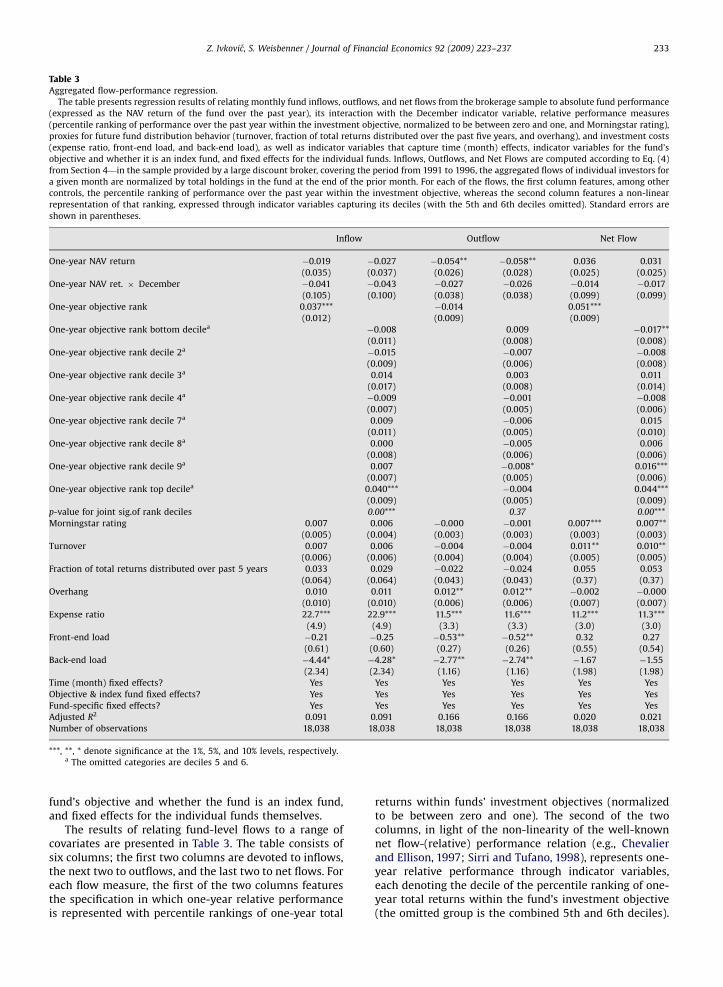
Table 3Aggregated flow-performance regression.

The table presents regression results of relating monthly fund inflows, outflows, and net flows from the brokerage sample to absolute fund performance

(expressed as the NAV return of the fund over the past year), its interaction with the December indicator variable, relative performance measures

(percentile ranking of performance over the past year within the investment objective, normalized to be between zero and one, and Morningstar rating),

proxies for future fund distribution behavior (turnover, fraction of total returns distributed over the past five years, and overhang), and investment costs

(expense ratio, front-end load, and back-end load), as well as indicator variables that capture time (month) effects, indicator variables for the fund’s

objective and whether it is an index fund, and fixed effects for the individual funds. Inflows, Outflows, and Net Flows are computed according to Eq. (4)

from Section 4—in the sample provided by a large discount broker, covering the period from 1991 to 1996, the aggregated flows of individual investors for

a given month are normalized by total holdings in the fund at the end of the prior month. For each of the flows, the first column features, among other

controls, the percentile ranking of performance over the past year within the investment objective, whereas the second column features a non-linear

representation of that ranking, expressed through indicator variables capturing its deciles (with the 5th and 6th deciles omitted). Standard errors are

shown in parentheses.

Inflow Outflow Net Flow

One-year NAV return �0.019 �0.027 �0.054** �0.058** 0.036 0.031

(0.035) (0.037) (0.026) (0.028) (0.025) (0.025)

One-year NAV ret. � December �0.041 �0.043 �0.027 �0.026 �0.014 �0.017

(0.105) (0.100) (0.038) (0.038) (0.099) (0.099)

One-year objective rank 0.037*** �0.014 0.051***

(0.012) (0.009) (0.009)

One-year objective rank bottom decilea�0.008 0.009 �0.017**

(0.011) (0.008) (0.008)

One-year objective rank decile 2a�0.015 �0.007 �0.008

(0.009) (0.006) (0.008)

One-year objective rank decile 3a 0.014 0.003 0.011

(0.017) (0.008) (0.014)

One-year objective rank decile 4a�0.009 �0.001 �0.008

(0.007) (0.005) (0.006)

One-year objective rank decile 7a 0.009 �0.006 0.015

(0.011) (0.005) (0.010)

One-year objective rank decile 8a 0.000 �0.005 0.006

(0.008) (0.006) (0.006)

One-year objective rank decile 9a 0.007 �0.008* 0.016***

(0.007) (0.005) (0.006)

One-year objective rank top decilea 0.040*** �0.004 0.044***

(0.009) (0.005) (0.009)

p-value for joint sig.of rank deciles 0.00*** 0.37 0.00***

Morningstar rating 0.007 0.006 �0.000 �0.001 0.007*** 0.007**

(0.005) (0.004) (0.003) (0.003) (0.003) (0.003)

Turnover 0.007 0.006 �0.004 �0.004 0.011** 0.010**

(0.006) (0.006) (0.004) (0.004) (0.005) (0.005)

Fraction of total returns distributed over past 5 years 0.033 0.029 �0.022 �0.024 0.055 0.053

(0.064) (0.064) (0.043) (0.043) (0.37) (0.37)

Overhang 0.010 0.011 0.012** 0.012** �0.002 �0.000

(0.010) (0.010) (0.006) (0.006) (0.007) (0.007)

Expense ratio 22.7*** 22.9*** 11.5*** 11.6*** 11.2*** 11.3***

(4.9) (4.9) (3.3) (3.3) (3.0) (3.0)

Front-end load �0.21 �0.25 �0.53** �0.52** 0.32 0.27

(0.61) (0.60) (0.27) (0.26) (0.55) (0.54)

Back-end load �4.44* �4.28* �2.77** �2.74** �1.67 �1.55

(2.34) (2.34) (1.16) (1.16) (1.98) (1.98)

Time (month) fixed effects? Yes Yes Yes Yes Yes Yes

Objective & index fund fixed effects? Yes Yes Yes Yes Yes Yes

Fund-specific fixed effects? Yes Yes Yes Yes Yes Yes

Adjusted R2 0.091 0.091 0.166 0.166 0.020 0.021

Number of observations 18,038 18,038 18,038 18,038 18,038 18,038

***, **, * denote significance at the 1%, 5%, and 10% levels, respectively.a The omitted categories are deciles 5 and 6.

Z. Ivkovic, S. Weisbenner / Journal of Financial Economics 92 (2009) 223–237 233

fund’s objective and whether the fund is an index fund,and fixed effects for the individual funds themselves.

The results of relating fund-level flows to a range ofcovariates are presented in Table 3. The table consists ofsix columns; the first two columns are devoted to inflows,the next two to outflows, and the last two to net flows. Foreach flow measure, the first of the two columns featuresthe specification in which one-year relative performanceis represented with percentile rankings of one-year total

returns within funds’ investment objectives (normalizedto be between zero and one). The second of the twocolumns, in light of the non-linearity of the well-knownnet flow-(relative) performance relation (e.g., Chevalierand Ellison, 1997; Sirri and Tufano, 1998), represents one-year relative performance through indicator variables,each denoting the decile of the percentile ranking of one-year total returns within the fund’s investment objective(the omitted group is the combined 5th and 6th deciles).

ARTICLE IN PRESS

Z. Ivkovic, S. Weisbenner / Journal of Financial Economics 92 (2009) 223–237234

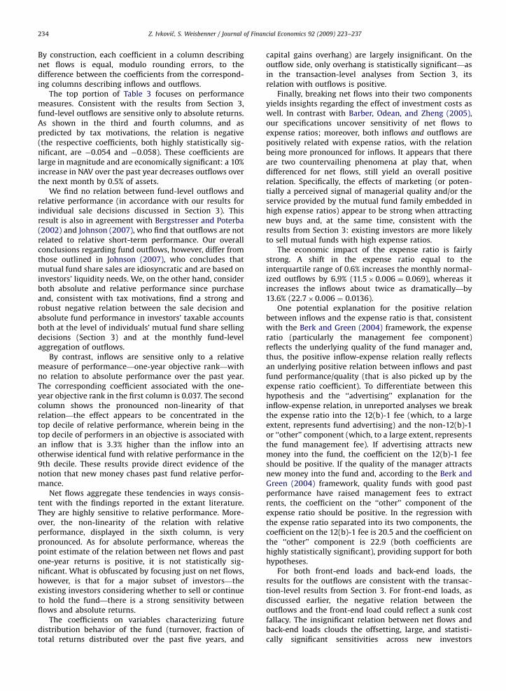
By construction, each coefficient in a column describingnet flows is equal, modulo rounding errors, to thedifference between the coefficients from the correspond-ing columns describing inflows and outflows.

The top portion of Table 3 focuses on performancemeasures. Consistent with the results from Section 3,fund-level outflows are sensitive only to absolute returns.As shown in the third and fourth columns, and aspredicted by tax motivations, the relation is negative(the respective coefficients, both highly statistically sig-nificant, are �0.054 and �0.058). These coefficients arelarge in magnitude and are economically significant: a 10%increase in NAV over the past year decreases outflows overthe next month by 0.5% of assets.

We find no relation between fund-level outflows andrelative performance (in accordance with our results forindividual sale decisions discussed in Section 3). Thisresult is also in agreement with Bergstresser and Poterba(2002) and Johnson (2007), who find that outflows are notrelated to relative short-term performance. Our overallconclusions regarding fund outflows, however, differ fromthose outlined in Johnson (2007), who concludes thatmutual fund share sales are idiosyncratic and are based oninvestors’ liquidity needs. We, on the other hand, considerboth absolute and relative performance since purchaseand, consistent with tax motivations, find a strong androbust negative relation between the sale decision andabsolute fund performance in investors’ taxable accountsboth at the level of individuals’ mutual fund share sellingdecisions (Section 3) and at the monthly fund-levelaggregation of outflows.

By contrast, inflows are sensitive only to a relativemeasure of performance—one-year objective rank—withno relation to absolute performance over the past year.The corresponding coefficient associated with the one-year objective rank in the first column is 0.037. The secondcolumn shows the pronounced non-linearity of thatrelation—the effect appears to be concentrated in thetop decile of relative performance, wherein being in thetop decile of performers in an objective is associated withan inflow that is 3.3% higher than the inflow into anotherwise identical fund with relative performance in the9th decile. These results provide direct evidence of thenotion that new money chases past fund relative perfor-mance.

Net flows aggregate these tendencies in ways consis-tent with the findings reported in the extant literature.They are highly sensitive to relative performance. More-over, the non-linearity of the relation with relativeperformance, displayed in the sixth column, is verypronounced. As for absolute performance, whereas thepoint estimate of the relation between net flows and pastone-year returns is positive, it is not statistically sig-nificant. What is obfuscated by focusing just on net flows,however, is that for a major subset of investors—theexisting investors considering whether to sell or continueto hold the fund—there is a strong sensitivity betweenflows and absolute returns.

The coefficients on variables characterizing futuredistribution behavior of the fund (turnover, fraction oftotal returns distributed over the past five years, and

capital gains overhang) are largely insignificant. On theoutflow side, only overhang is statistically significant—asin the transaction-level analyses from Section 3, itsrelation with outflows is positive.

Finally, breaking net flows into their two componentsyields insights regarding the effect of investment costs aswell. In contrast with Barber, Odean, and Zheng (2005),our specifications uncover sensitivity of net flows toexpense ratios; moreover, both inflows and outflows arepositively related with expense ratios, with the relationbeing more pronounced for inflows. It appears that thereare two countervailing phenomena at play that, whendifferenced for net flows, still yield an overall positiverelation. Specifically, the effects of marketing (or poten-tially a perceived signal of managerial quality and/or theservice provided by the mutual fund family embedded inhigh expense ratios) appear to be strong when attractingnew buys and, at the same time, consistent with theresults from Section 3: existing investors are more likelyto sell mutual funds with high expense ratios.

The economic impact of the expense ratio is fairlystrong. A shift in the expense ratio equal to theinterquartile range of 0.6% increases the monthly normal-ized outflows by 6.9% (11.5�0.006 ¼ 0.069), whereas itincreases the inflows about twice as dramatically—by13.6% (22.7�0.006 ¼ 0.0136).

One potential explanation for the positive relationbetween inflows and the expense ratio is that, consistentwith the Berk and Green (2004) framework, the expenseratio (particularly the management fee component)reflects the underlying quality of the fund manager and,thus, the positive inflow-expense relation really reflectsan underlying positive relation between inflows and pastfund performance/quality (that is also picked up by theexpense ratio coefficient). To differentiate between thishypothesis and the ‘‘advertising’’ explanation for theinflow-expense relation, in unreported analyses we breakthe expense ratio into the 12(b)-1 fee (which, to a largeextent, represents fund advertising) and the non-12(b)-1or ‘‘other’’ component (which, to a large extent, representsthe fund management fee). If advertising attracts newmoney into the fund, the coefficient on the 12(b)-1 feeshould be positive. If the quality of the manager attractsnew money into the fund and, according to the Berk andGreen (2004) framework, quality funds with good pastperformance have raised management fees to extractrents, the coefficient on the ‘‘other’’ component of theexpense ratio should be positive. In the regression withthe expense ratio separated into its two components, thecoefficient on the 12(b)-1 fee is 20.5 and the coefficient onthe ‘‘other’’ component is 22.9 (both coefficients arehighly statistically significant), providing support for bothhypotheses.

For both front-end loads and back-end loads, theresults for the outflows are consistent with the transac-tion-level results from Section 3. For front-end loads, asdiscussed earlier, the negative relation between theoutflows and the front-end load could reflect a sunk costfallacy. The insignificant relation between net flows andback-end loads clouds the offsetting, large, and statisti-cally significant sensitivities across new investors

ARTICLE IN PRESS

Table 4Differences by tax status of outflows.

The table presents regression results of relating monthly fund outflows from the brokerage sample to absolute fund performance (expressed as the NAV

return of the fund over the past year), its interaction with the December indicator variable, relative performance measures (percentile ranking of

performance over the past year within the investment objective normalized to be between zero and one, and Morningstar rating), proxies for future fund

distribution behavior (turnover, fraction of total returns distributed over the past five years, and overhang), and investment costs (expense ratio, front-end

load, and back-end load), as well as indicator variables that capture time (month) effects, indicator variables for the fund’s objective and whether it is an

index fund, and fixed effects for the individual funds. Outflows are computed according to Eq. (4) from Section 4—in the sample provided by a large

discount broker, covering the period from 1991 to 1996, the aggregated flows of individual investors for a given month are normalized by total holdings in

the fund at the end of the prior month. Aside from the outflows computed across all accounts, we also compute outflows from taxable and tax-deferred

accounts. Panel A features the percentile ranking of performance over the past year within the investment objective, whereas Panel B features a non-linear

representation of that ranking, expressed through indicator variables capturing its deciles (with the 5th and 6th deciles omitted). Within each panel, the

first column features outflows from all accounts (and is thus a restatement of the results from Table 3), the next two columns focus on outflows from

taxable and tax-deferred accounts, respectively, and the last column reports the differences between the two. Standard errors are shown in parentheses.

Panel A: Linear model of relative performance Panel B: Non-linear model of relative performance

All accounts

combined

Separate consideration of taxable and tax-

deferred accounts

All accounts

combined

Separate consideration of taxable and tax-

deferred accounts

Taxable

accounts

Tax-deferred

accounts

Difference Taxable

accounts

Tax-deferred

accounts

Difference

One-year NAV return �0.054** �0.293*** 0.020 –0.313*** –0.058** –0.295*** 0.018 –0.313***

(0.026) (0.089) (0.014) (0.092) (0.028) (0.088) (0.014) (0.090)

One-year NAV ret. x Dec. –0.027 –0.048 –0.009 –0.039 –0.026 –0.047 –0.009 –0.038

(0.038) (0.119) (0.032) (0.123) (0.038) (0.119) (0.033) (0.124)

One-year objective rank –0.014 –0.029 –0.003 –0.026

(0.009) (0.019) (0.007) (0.019)

One-year objective rank

bottom decilea

0.009 0.019 0.016** 0.002

(0.008) (0.021) (0.007) (0.022)

One-year objective rank

decile 2a

–0.007 0.009 0.006 0.003

(0.006) (0.013) (0.005) (0.014)

One-year objective rank

decile 3a

0.003 –0.001 0.006 –0.006

(0.008) (0.010) (0.008) (0.013)

One-year objective rank

decile 4a

–0.001 –0.001 0.010 –0.011

(0.005) (0.010) (0.007) (0.011)

One-year objective rank

decile 7a

–0.006 –0.003 –0.004 0.007

(0.005) (0.011) (0.004) (0.012)

One-year objective rank

decile 8a

–0.005 –0.007 0.004 –0.010

(0.006) (0.007) (0.004) (0.008)

One-year objective rank

decile 9a

–0.008* –0.012 0.006 –0.019

(0.005) (0.009) (0.004) (0.012)

One-year objective rank top

decilea

–0.004 –0.012 0.010 –0.022

(0.005) (0.010) (0.007) (0.016)

p-value for joint sig. of rank

deciles

0.37 0.48 0.27 0.32

Other controls from Table 3? Yes Yes Yes Yes Yes Yes Yes Yes

Adjusted R2 0.166 0.218 0.080 0.088 0.166 0.080 0.088 0.190

Number of observations 18,038 15,136 14,044 29,180 18,038 15,136 14,044 29,180

***, **, * denote significance at the 1%, 5%, and 10% levels, respectively.a The omitted categories are deciles 5 and 6.

Z. Ivkovic, S. Weisbenner / Journal of Financial Economics 92 (2009) 223–237 235

(inflows) and old investors (outflows). Back-end loads areassociated with less new money entering the fund; at thesame time, they are also associated with the existingmoney being less prone to leave.

In sum, many of the rich characterizations of investorsensitivities to various fund characteristics discussedabove are obscured when inflows and outflows arecombined and only net flows are studied. Our resultsstress that the absence of a relation between net flows and

a fund characteristic does not imply that the characteristicis unimportant for all investors. Indeed, given that new orpotential investors in the fund and the incumbentinvestors may have different considerations, disentanglingnet flows into its components is important. Thus, whenassessing the overall effect of a fund-policy change, it isrelevant to understand the differing sensitivities of new orpotential investors and existing investors who alreadyown shares.

ARTICLE IN PRESS

Z. Ivkovic, S. Weisbenner / Journal of Financial Economics 92 (2009) 223–237236

4.2. Robustness check: separating outflows into outflows in

taxable and tax-deferred accounts

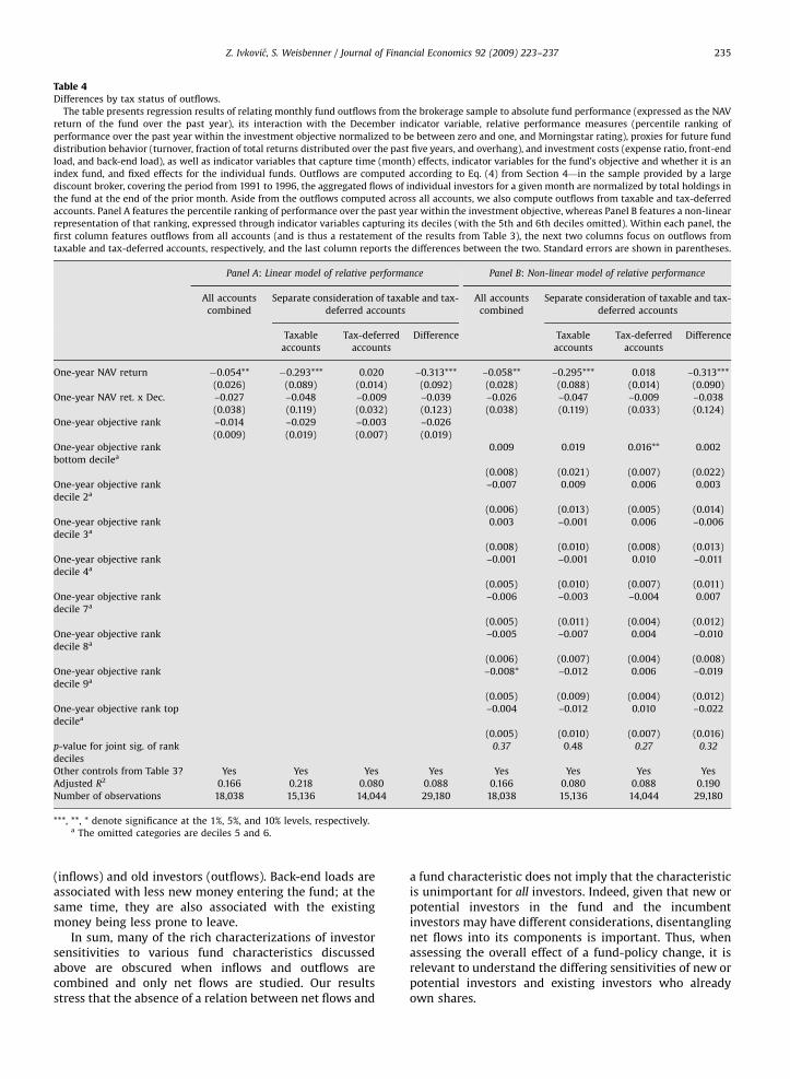
This section features the last robustness check. Resultsconcerning the relation between outflow and perfor-mance, presented in detail in Section 4.1, suggest thatthe relation between outflows and performance is bestcharacterized by a pronounced role of tax motivations fortrade. Because our data enable us to disentangle outflowsfrom taxable and tax-deferred accounts, we can assessthis hypothesis even more directly—if tax motivations aredriving the result for outflows, then absolute performanceshould matter only in the context of outflows from taxableaccounts. We carry out this robustness check and reportthe results in Table 4. For brevity, we report only theregression coefficients related to absolute and relativeone-year performance.

Table 4 is divided into two panels. Panel A employs asimpler, linear model of relative performance, and Panel Bemploys a non-linear representation of relative perfor-mance, as was done in Table 3. The first column of eachpanel features the regression results estimated over thefund outflows aggregated over all accounts. Thus, the firstcolumn in Panel A (Panel B) corresponds to the third(fourth) column in Table 3. The next two columns in eachpanel feature regression results estimated for the outflowscomputed from taxable accounts only and tax-deferredaccounts only, respectively, and the last column in eachpanel features the difference between the two.

This robustness test of the hypothesis that tax motiva-tions drive the relation between outflows and absoluteperformance affirms that interpretation very strongly. Asin Table 3, there is no ‘‘action’’ in the domain of relativeperformance in either taxable or tax-deferred accounts.This is true for both the linear specifications (Panel A) andthe nonlinear specifications (Panel B).13 Absolute perfor-mance, the central theme of this section, displays thepredicted pattern: it is substantially larger in magnitudefor outflows from taxable accounts (�0.293 or �0.295,depending upon the specification) than for outflows fromtax-deferred accounts (0.020 or 0.018, depending uponthe specification), and is statistically significant only forthe taxable accounts.

Although not reported in the table for brevity, we alsotest whether the other variables in the outflow regressions(the proxies for future fund distributions and the mutualfund costs) have statistically different effects for taxableoutflows than they do for tax-deferred outflows. There areno statistically significant differences across the coeffi-cients in the taxable and tax-deferred regressions, withthe exception of three variables—the past one-yearabsolute return (as discussed above), turnover, and over-hang. Both the relation between outflows and turnoverand the relation between outflows and overhang arestronger for taxable outflows (with both differences

13 Among the results of the non-linear specifications, one relative-

performance coefficient—associated with the bottom decile in tax-

deferred accounts—does attain statistical significance, but the p-value of

the joint significance of all of the relative rank deciles is 0.27.

statistically significant at the 5% level). This is consistentwith these proxies for future fund distributions affectingfund outflows because they may carry with them highertax liabilities.

5. Conclusion

This paper studies the determinants of mutual fundflows, with particular attention to individual investors’mutual fund selling decisions. In stark contrast withinvestor behavior regarding common stocks, there is astrong negative relation between the probability of saleand past mutual fund performance. Individuals hold on tomutual fund shares that have appreciated since purchaseand are willing to sell those that have incurred losses. Bycomparing trading patterns in taxable and tax-deferredaccounts, we confirm that the negative relation can beexplained by tax-motivated trading.

Among a mutual fund’s choice variables are howreturns should be distributed to investors, with implica-tions for taxable investments, and what kinds of fees—

expenses and loads—should be charged. Both haveimplications for outflows from the fund. The evidence oftax-motivated trading in taxable accounts encompassesnot only the negative relation between propensity to selland NAV change since purchase, but also increasedpropensity to sell in response to three other variablesthat signal potential future tax liabilities—fund turnover,past distribution behavior of the fund, and capital gainsoverhang. Thus, individuals seem to be sensitive not onlyto direct tax considerations such as what taxes would beincurred in the event of selling the mutual fund, but toindirect tax considerations such as future distributions.

In regard to investment costs, somewhat surprisingly,investors from our sample seem to view front-end chargesas impediments to sale. On the other hand, high expenseratios (an ongoing, not-in-your-face cost) are associatedwith a substantial increase in the probability of redemp-tion, particularly if the expense ratio has increased sincethe investor purchased the fund.

Finally, we also use the brokerage data to aggregateindividuals’ purchases and redemptions into fund-levelmonthly measures of inflows and outflows and study thedeterminants of flows for inflows, outflows, and net flows.We find that, broadly speaking, inflows are driven byfunds’ relative performance measures, that is, funds’ one-year performance relative to other funds pursuing thesame objective. This suggests that new money indeedchases the best performers in an objective, with norelation to the fund’s ‘‘absolute’’ performance. On theother hand, consistent with tax motivation and pro-nounced only in taxable accounts, outflows are drivenby funds’ one-year absolute returns. Thus, breaking netflows into their two components yields important insightson the behavior of old and new money.

References

Barber, B., Odean, T., 2000. Trading is hazardous to your wealth: thecommon stock investment performance of individual investors.Journal of Finance 55, 773–806.

ARTICLE IN PRESS

Z. Ivkovic, S. Weisbenner / Journal of Financial Economics 92 (2009) 223–237 237

Barber, B., Odean, T., Zheng, L., 2005. Out of sight, out of mind: the effectsof expenses on mutual fund flows. Journal of Business 78,2095–2119.

Bergstresser, D., Poterba, J., 2002. Do after-tax returns affect mutual fundinflows. Journal of Financial Economics 63, 381–414.

Berk, J., Green, R., 2004. Mutual fund flows and performance in rationalmarkets. Journal of Political Economy 112, 1269–1295.

Cashman, G., Deli, D., Nardari, F., Villupuram, S., 2006. Investors dorespond to poor mutual fund performance: Evidence from inflowsand outflows. Working Paper, Arizona State University.

Chevalier, J., Ellison, G., 1997. Risk taking by mutual funds as a responseto incentives. Journal of Political Economy 105, 1167–1200.

Edelen, R., 1999. Investor flows and the assessed performance of open-end mutual funds. Journal of Financial Economics 53, 439–466.

Frazzini, A., 2006. The disposition effect and under-reaction to news.Journal of Finance 61, 2017–2046.

Grinblatt, M., Keloharju, M., 2001. What makes investors trade? Journalof Finance 56, 589–616.

Han, A., Hausman, J., 1990. Flexible parametric estimation of durationand competing risk models. Journal of Applied Econometrics 5, 1–28.

Investment Company Institute, 2004. Mutual Fund Factbook: A Guide ToTrends And Statistics In The Mutual Fund Industry, 43rd ed.

Ippolito, R., 1992. Consumer reaction to measures of poor quality:evidence from the mutual fund industry. Journal of Law andEconomics 35, 45–70.

Ivkovic, Z., Poterba, J., Weisbenner, S., 2005. Tax-motivated trading byindividual investors. American Economic Review 95, 1605–1630.

Johnson, W., 2007. Who monitors the mutual fund manager, new or oldshareholders? Working Paper, University of Oregon.

Kahneman, D., Tversky, A., 1979. Prospect theory: an analysis of decisionunder risk. Econometrica 47, 263–291.

Keswani, A., Stolin, D., 2008. Which money is smart? Mutual fund buysand sells of individual and institutional investors. Journal of Finance63, 85–118.

Meyer, B., 1990. Unemployment insurance and unemployment spells.Econometrica 58, 757–782.

Odean, T., 1998. Are investors reluctant to realize their losses? Journal ofFinance 53, 1775–1798.

O’Neal, E., 2004. Purchase and redemption patterns of U.S. equity mutualfunds. Financial Management 33, 63–90.

Shefrin, H., Statman, M., 1985. The disposition to sell winners too earlyand ride losers too long: theory and evidence. Journal of Finance 40,777–792.

Sirri, E., Tufano, P., 1998. Costly search and mutual fund flows. Journal ofFinance 53, 1589–1622.