Embed Size (px)
Citation preview

Taxes and the present value assessment of economic losses in personal injury litigation: Comment1
Scott Gilbert Economics Department
Southern Illinois University Carbondale Carbondale, IL 62901
e-mail: [email protected], office phone: (618) 453-5095
cell phone: (618) 319-2465, fax: (618) 453-2717
August 8, 2012
1 For helpful comments on the present work I thank participants at the annual national meeting of the American
Academy of Economic and Financial Experts (Las Vegas, 2012).

2
Taxes and the present value assessment of economic losses in personal injury litigation: Comment Abstract Anderson and Barber (2010) provide a recent discussion of tax effects on economic damages, for forensic economists and similar experts who supply the courts with opinions on economic damages. Anderson and Barbers’ paper fills a void in the forensic economics literature, by offering a formal theory of how tax considerations can impact economic damages. In the present work I point out a limitation of this theory - via a counter-example, and discuss conditions under which which the theory seems to hold approximately. Keywords: income stream; present value; tax; personal injury; wrongful death

I. Introduction
In court cases involving personal injury and wrongful death, economic damages typically the present
value of future incomes which would have been earned – if not for the injury or death. For the typical
U.S. worker, it is natural for their income to grow over most of their worklife due to inflation and
increases in productivity. When valuing a growing income stream, the forensic economist (FE) has
various factors to consider, including the inclusion or exclusion of tax -- in the worker’s wages and also in
interest income associated with the investment fund required to replicate lost future wages. The FE
determines whether or not to include tax or not depending on legal requirements of the court in which
the case is filed, and on the FE’s opinion about the reasonableness of pre-tax vs. post-tax values. In cases
where the treatment of tax is subject to the FE’s choice, it is important to be able to explain the
consequences of such choices to the court. Does the inclusion of tax tend to raise economic damage
estimates, or not? Economic theory is a potentially valuable resource for forensic economists who wish
to be able to answer this question confidently at trial and in deposition.
In terms of economic theory, the effect of tax on the present value of a growing income stream has not
been addressed in the general economics literature. Over the last 25 years forensic economists have
published research in journals specialized to their field, including the Journal of Forensic Economics and
the Journal of Legal Economics. In both journals, a number of research papers have discussed tax and
present value. In the Journal of Forensic Economics, this includes some early work by Goodwin and Paul
(1988) and Ciecka (1989), and a special issue in 1994 (volume 7, number 3) devoted to the subject of tax
and economic awards. In the Journal of Legal Economics, the recent work of Gary Anderson and Joel
Barber (2010) makes a number of contributions to the literature, including a discussion of tax effects on

2
the present value of services and medical care. It also surveys the existing literature, and posits a
theoretical relationship between tax and the present value of growing income.
Anderson and Barber (2010) posit that tax has a negative effect on the present value of growing income
when the number future pay periods is small, and has a positive effect when the number of periods is
large. They also provide a mathematical formula for the “breakeven” point -- the number of periods at
which the tax effect switches from negative to positive. This theoretical work is insightful and extends
the scope of the forensic economics literature.
The present work reconsiders the effect of tax on the present value of growing income. I show by
counter-example that the Anderson and Barber (2010) tax theory does not generally hold in the
mathematical form in which they state it, and I identify the source of error. I also provide examples
where their breakeven formula is nearly correct, giving some hints for future research on the effects of
tax on economic damages.
II. Anderson and Barber (2010)
Anderson and Barber (2010), henceforth abbreviated AB, analyze the effect of tax on the present value
of earnings, under the assumption that earnings grow at a constant rate g over time:
(2.1) 0(1 )t
tE E g
with 0E the base earnings earned in period 0. Anderson and Barber posit an interesting theory about
how tax affects the present value of earnings. I briefly summarize their results in Section II.A, then
examine them in more detail in Sections II.B-II.C.

3
A. Tax Effect
Anderson and Barber (2010) use the following notation and formulas for the present value of earnings,
with and without tax:
(2.2) 0 (1 )(1 ) 11
( (1 ) ) 1 (1 )
Ne
earningsaftertax i i
E g gPV
r g r
(2.3) 0 (1 ) 1
)
( 1
1
N
earningswithouttax
E g gPV
r g r
where r is the interest rate on a (riskless) bond, e is the tax rate on earnings, and i is the tax rate on
interest.
In terms of tax effects, AB posit a breakeven point, such that tax has a negative effect on present value
when the number of earnings periods is less than some value which I will call *N , and has a positive
effect on present value when the number of periods exceeds *N . In other words, they posit that
earningsaftertaxPV is smaller than earningswithouttaxPV when N is small, and that the reverse relationship holds
when N is large. They identify the breakeven point via the following equation:
(2.4) (1 )
ie rD
r
where D is the constant:

4
(2.5)
1
(1 ) 1
( ) 11
1
N
N
gN
r rD
r g g
r
According to AB, for smaller N the left-hand side of (2.4) is larger than the right-hand side, and the
after-tax present value of earnings is less than the without-tax present value. For larger N , the left-hand
side is smaller than the right-hand side, and the after-tax present value of earnings is greater than the
without-tax present value.
B. (Counter)Example
Anderson and Barber provide an example to illustrate their mathematical theory. They set the tax rate
on earnings equal to that on interest, with 0.1e i , and they set the growth rate on earnings equal
to the before-tax rate of interest, with 0.05g r . They find that the breakeven condition (2.4) holds
with 21D and that this value of D is achieved at 40N . They conclude that, for the given values
of , , eg r and i , adjustment for tax will result in a decrease in the present value of loss with the
introduction of taxes in situations where 40N , and will increase the present value of loss in
situations where 40N .
Examining the present value formulas (2.2)-(2.3) and the definition (2.5) of the constant D , some
trouble arises. Since the difference r g equals 0, the without-tax present value (2.3) and the formula
(2.5) for D are undefined. Neither can be a finite quantity, as both involve division by zero. Also, they
can not be reliably assigned the value plus infinity (+ ) or minus infinity (- ), as both values emerge in
the limit as we let r g converge to zero from above or, alternatively, from below. Consequently, it is

5
not possible to check the breakeven condition (2.4) in Example 1 via these formulas, or to apply this
condition to the determination of tax effects.
While formulas and (2.3) and (2.5) do not apply in this example, Anderson and Barber provide
alternative formulas that do, these being:
(2.6) 0
1
(1 )
(1 )
iN
earningswithouttax it
E gPV
r
and:
(2.7)
0
1
0
1
(1 )
(1 )
(1 )
(1 )
tN
tt
tN
tt
tE g
rD
E g
r
which are well-defined for any positive values of g , r , and 0E . To check the posited value -21 for D , I
apply the AB breakeven condition (2.4) to get:
(2.8) (1 )
21e
i
rD
r
which matches their result.
We can also check the posited value 40 for the number N of future work periods. Given the value for
D , I solve for N by applying the formula (2.7) with total offset ( g r ):

6
(2.9) 1
1
1
N
t
N
t
t
D
(2.10) ( 1) / 2N N
N
(2.11) 1
2
N
The value *N of N that satisfies the breakeven condition (2.4) when e i is then:
(2.12) * 21N
r
With 0.05r , (2.12) yields * 41N , which is nearly the same as the value 40 mentioned by Anderson
and Barber.
Turning now to the posited tax effects, I compute present values and report them in Table 1, with base
earnings 0E set equal to 1. At each horizon N , present value without tax equals N due to total offset.
At 39N , PV without tax is larger than PV with tax, hence tax lowers present value. The same is
true at 40N through 42, whereas Anderson and Barber suggest that for N larger than 40 (or 41) tax
should raise present value. At 43N tax raises PV , hence if there is a breakeven value of N at which
the tax effect goes from negative to positive, it is 42 or 43, which is inconsistent with AB's breakeven
condition (2.4).

7
C. Other Evidence
To further examine the workability of the breakeven condition (2.4) for tax effects, consider some more
examples. As earlier, let there be total offset between the growth rate on earnings and the interest rate,
with 0.05g r , and let the tax rate on earnings be equal to the tax rate on interest. The breakeven
value *N of the earnings horizon N , which I derived earlier, is again * 41N here because r has not
changed.
Table 2 reports present values with and without tax, analogous to Table 1, but with a lower tax rate:
0.01 . As shown, tax lowers present value at 39,40,41N , and raises it at 42,43,44N , which
is consistent with Anderson and Barbers' posited tax effects. A possible explanation is that their theory is
applicable when tax rates are sufficiently small, but not for all tax rates. As a further check, I report in
Table 3 results for a high tax rate: 0.5 . Here the discrepancy between posited tax effects and actual
effects is dramatic. Tax lowers present values at 39,,40,...,51N , and raises present values for
52,53,54N , hence if there is a breakeven value of N it must be between 51 and 52, rather than the
value * 41N .
Based on the foregoing examples, a possibility is that there is a breakeven value for N which increases
with the tax rate . In support of this idea, Table 4 reports breakeven possibilities for N at the tax
rates 0.01,0.05,0.1,0.2,...,0.5 . At each stated value of N , tax lowers present value for nearby
smaller values of N , and raises present value for nearby larger values of N . As indicated, these
candidate breakeven values are increasing in the tax rate.

8
III. Forensics
To explain the pattern of observed discrepancies between actual tax effects and those postulated by
Anderson and Barber (2010), let's consider the arguments underlying them. The crux of the matter is the
breakeven condition (2.4), which for AB represents a balancing of offsetting effects: on the left-hand
side of (2.4) is a loss of present value associated with tax on income, while on the right-hand side is a
gain in present value associated with tax on interest. The validity of this balancing act is not obvious, and
involves some reasoning in terms of elasticities and also the constant D .
Anderson and Barber refer to D as duration, but if duration refers to time then it should be positive, or
at least non-negative, whereas Anderson and Barbers' D is always negative. As a first step in
reconsidering the breakpoint condition (2.4) I discuss the concept of duration, then turn to elasticities
and the marginal analysis of offsetting tax effects.
A. Duration
Anderson and Barber identify the constant D as duration in the sense of Macaulay (1938). To get a
sense of what Macaulay means by duration in this work, here is a quote -- Macaulay (1938, Chapter 2,
page 48):
Now, if present value weighting be used, the 'duration' of a bond is an average of the durations of the separate single payment loans into which the bond may be broken up. To calculate this average the duration of each individual single payment loan must be weighted in proportion to the size of the individual loan; in other words, by the ratio of the present value of the individual future payment to the sum of all the present values, which is, of course, the price paid for the bond.
For a riskless bond paying a coupon amount I in future periods 1, 2,..., N , and returning a face value
F in period N , with gross yield 1R r , Macaulay computes his duration D as follows:

9
(3.1) 2
2
2N N
N N
I I NI NF
R R R RDI I I F
R R R R
This D is a weighted average of the dates 1, 2,...., N , and as such its value lies between the values 1
and N , a positive value.
While Macaulay (1938) focuses on bonds, his concept of duration -- as a present-value weighted average
of payment dates -- is applicable to any known positive income stream over future dates 1,2,...,t N :
(3.2) 1
Nt
t
PVD t
PV
with total present value PV andtPV the present value of the earnings arriving in year t . For additional
discussion of Macaulay's duration, see Weil (1973).
Applied to the bond example (3.1), the general duration formula (3.2) has the following components:
(3.3) 2 N N
I I I FPV
R R R R
(3.4) 1
IPV
R
(3.5) 2 2
IPV
R
and so on, until:
(3.6) 1 1N N
IPV
R

10
(3.7) N N
I FPV
R
For a general earnings stream 1,..., NE E , the (pre-tax) present value of income arriving in future period
t is:
(3.8) (1 )
tt t
EPV
r
and Macaulay's duration is:
(3.9) 1
1
(1 )
(1 )
Nt
tt
Nt
tt
tE
rD
E
r
Macaulay (1938, page 51) illustrates bond duration by computing it for a variety of bonds with different
yields and years to maturity. In Table 5 I report duration for growing income streams, with D computed
via formula (3.9) and earnings growth rate 0.05g . As in Macaulay's work, all duration values are
positive. In the last row of Table 5 I report results in the limit case where horizon N approaches infinity.
For the cases g r it is easy to show that D as N . For the case g r I use Anderson and
Barbers' D formula (2.5), multiplied times -1.
John Hicks (1939, page 186) independently develops the duration formula (3.9), which he calls the
“average period” of the income stream. Again, duration is a measure of time, hence is non-negative.
Popular software for financial calculations, including Microsoft Excel 2010 and Wolfram Mathematica 8,
implement duration in these terms. For example, consider a 5 year bond that pays no coupon and has

11
an interest rate of 10 percent. Its only payment is at the end of 5 years, so Macaulay's duration is 5D
in accordance with the following Excel function: =duration(01/01/10,1/1/2015,0,0.1,1).
Could the errors generated by Anderson and Barbers' postulated tax effects be due to a wrong sign --
negative rather than positive -- for their Macaulay duration formula? The answer turns out to be “no,”
the reason being that if we replace Anderson and Barbers' constant D with its negative D in the
breakeven formula (2.4), we get a new formula which can't work unless the negative sign on the right-
hand side is itself reversed -- otherwise the positive value on the left-hand side can not match a positive
sign on the right-hand side -- which then reverts to the original formula. Despite this fact, it is helpful to
have some understanding of Macaulay's duration, as it plays an integral part in Anderson and Barbers'
basic argument motivating the breakeven condition (2.4). This argument involves elasticities, and as
shown in the next section the argument is not quite right. It does however contain useful elements, and
to appreciate these fully it will be helpful to note here that, according to Hicks (1939), the duration
formula (3.9) can also be interpreted as the elasticity of present value with respect to the “discount
factor” 1/ R . That is, with present value expressed as:
(3.10) 1
Nt
t
t
PV R E
and its elasticity defined as:
(3.11) PV R
R PV

12
Hicks shows that elasticity (3.11) is given by the duration formula (3.9).
B. Elasticity and Marginal Analysis
Consider now the marginal analysis of tax effects. If the negative effect of income tax just offsets the
positive effect of interest tax on present value then, at the margin, the change dPV in present value
equals 0:
(3.12) 0e i
e i
PV PVdPV d d
Suppose, moreover, that the earnings tax rate e grows at the same instantaneous rate as does the tax
rate i on interest:
(3.13) e i
e i
d d
Then we can then interpret the marginal condition (3.12) on present value in terms of elasticities:
(3.14) e i
e i
PV PV
PV PV
The elasticity of (after-tax) PV with respect to the earnings tax rate is:
(3.15) 1
e e
e e
PV
PV

13
For a small tax rate e on earnings, we can approximate this elasticity as follows:
(3.16) e
ee
PV
PV
On the other hand, the elasticity of PV with respect to the interest tax rate is:
(3.17) (1 (1 ))
(1 (1 ))
i i i
i i i
PV PV r
PV r PV
(3.18) 1 (1 )
1 (1 ) (1 (1 ))
i
i
i i
r PV r
r r PV
(3.19) 1 (1 )
iaftertaxi
rD
r
with aftertaxD the variant of Macaulay-Hicks duration D based on after-tax earnings and interest:
(3.20) 1
1
(1 )
(1 (1 ) )
(1 )
(1 (1 ) )
eNt
i tt
aftertax eNt
i tt
t E
rD
E
r
The step (3.19) follows from Hicks' elasticity result mentioned earlier. If the tax rates are close to zero
then after-tax duration is about the same as before-tax duration:

14
(3.21) aftertaxD D
Applying the small-tax approximations (3.16) and (3.21), the balancing condition (3.12) is approximately:
(3.22) 1
ie r
Dr
which is the Anderson and Barber breakeven condition (2.4) restated as a small-tax approximation. A
minus (-) sign appears on the right-hand side of (2.4) but not (3.22). This difference in sign reflects the
difference between the Anderson and Barber constant D and Macaulay-Hicks duration D .
The upshot of these analytics is that Anderson and Barbers’ mathematical formulation of a “breakpoint”
- for signing tax effects – seems to be a workable approximation when the relevant tax rate is sufficiently
small. If so it should be possible to confirm their mathematical theory as a locally valid, in the
neighborhood of a zero tax rate, though a rigorous confirmation of this sort exceeds the present scope.
IV. Concluding Remarks
The present work reconsiders the effect of tax on the present value of future growing income streams,
by discussing a mathematical theory proposed by Gary Anderson and Joel Barber (2010). These authors
posit that an increase in the tax rate on both earnings and interest income will lower the present value
of income streams if the work period is sufficiently short, but will raise present value if the work period
is sufficiently long. Moreover, they propose an exact “breakeven” point – a formula for the length of
work period at which the tax effect switches from negative to positive. The present research points out
15
that Anderson and Barbers’ breakeven formula is not generally valid, but does seem to be a good
approximation when the tax rate is sufficiently small.
Future research should be directed to the question of whether or not Anderson and Barbers’ general
conception of tax effects (on the present value of growing income streams) is valid: is there a breakeven
point at which tax effects switch from negative to positive, as the work period lengthens? While a
general formula for such a breakpoint is unknown, the small-tax approximation sketched in the present
work provides a tentative starting point.
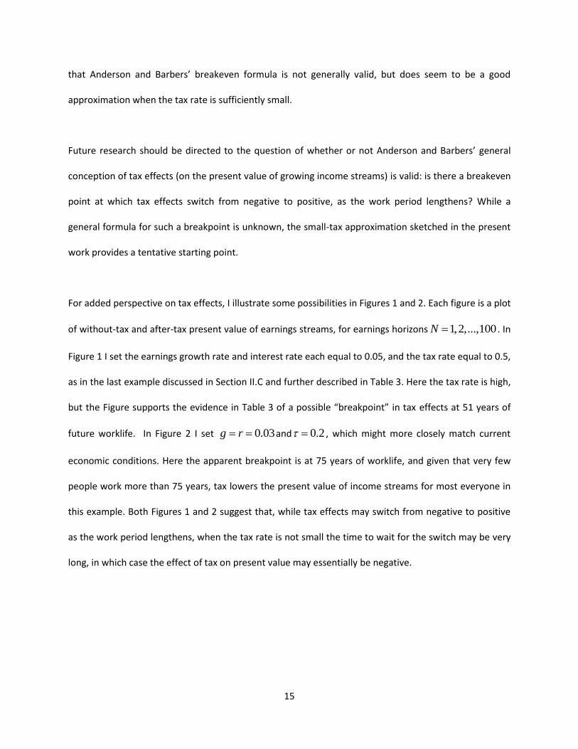
For added perspective on tax effects, I illustrate some possibilities in Figures 1 and 2. Each figure is a plot
of without-tax and after-tax present value of earnings streams, for earnings horizons 1,2,...,100N . In
Figure 1 I set the earnings growth rate and interest rate each equal to 0.05, and the tax rate equal to 0.5,
as in the last example discussed in Section II.C and further described in Table 3. Here the tax rate is high,
but the Figure supports the evidence in Table 3 of a possible “breakpoint” in tax effects at 51 years of
future worklife. In Figure 2 I set 0.03g r and 0.2 , which might more closely match current
economic conditions. Here the apparent breakpoint is at 75 years of worklife, and given that very few
people work more than 75 years, tax lowers the present value of income streams for most everyone in
this example. Both Figures 1 and 2 suggest that, while tax effects may switch from negative to positive
as the work period lengthens, when the tax rate is not small the time to wait for the switch may be very
long, in which case the effect of tax on present value may essentially be negative.

16
References Anderson, Gary A., and Joel R. Barber (2010). Taxes and the present value assessment of economic losses in personal injury litigation, Journal of Legal Economics 17, 1-28. Ciecka, James (1989). The consideration of progressive taxes in present value calculations for personal injury and wrongful death cases: Comment. Journal of Forensic Economics 2(2), 3-6. Goodwin, Randall and Chris Paul (1988). The consideration of progressive taxes in present value calculations for personal injury and wrongful death cases. Journal of Forensic Economics 1(1), 83-91. Hicks, John R. (1939). Value and Capital (Oxford: Clarendon Press). Macaulay, Frederick R. (1938). Some theoretical problems suggested by the movements of interest rates, bond yields , and stock prices in the United States since 1856 (Columbia University Press for the National Bureau of Economic Research). Weil, Roman L. (1973). Macaulay's duration: An appreciation. Journal of Business 46(4), 589-592.

17
Table 1: Present values, Tax Rate = 10 percent
PV PV
N without tax with tax
39 39 38.67
40 40 39.76
41 41 40.86
42 42 41.96
43 43 43.06
44 44 44.17
Table 2: Present values, Tax Rate = 1 percent
PV PV
N without tax with tax
39 39 38.980
40 40 39.989
41 41 40.999
42 42 42.009
43 43 43.019
44 44 44.030

18
Table 3: Present values, Tax Rate = 50 percent
PV PV
N without
tax with tax
39 39 32.749
40 40 34.060
41 41 35.403
42 42 36.780
43 43 38.190
44 44 39.630
45 45 41.110
46 46 42.630
47 47 44.180
48 48 45.770
49 49 47.400
50 50 49.060
51 51 50.770
52 52 52.520
53 53 54.320
54 54 56.150
55 55 58.035
56 56 59.962
Table 4: Breakeven Possibilities
tau 0.01 0.05 0.1 0.2 0.3 0.4 0.5
breakpoint possibility 41 42 43 44 47 49 52

19
Table 5: Duration
horizon r=4% r=5% r=6%
1 1.000 1.000 1.000
3 2.006 2.000 1.994
6 3.528 3.500 3.472
10 5.579 5.500 5.422
15 8.179 8.000 7.823
25 13.497 13.000 12.508
50 27.485 25.500 23.533
100 58.355 50.500 42.718
infinity infinity infinity 106.000
20
Figure 1: Present Value of Income Stream ( .05r g , .5 )
0
40
80
120
160
200
240
10 20 30 40 50 60 70 80 90 100
PV_TAX PV_NOTAX

21
Figure 2: Present Value of Income Stream, ( .03r g , .20 )
0
20
40
60
80
100
120
10 20 30 40 50 60 70 80 90 100
PV_TAX PV_NOTAX