Journal of Biomedical Informatics 53 (2015) 15–26

Contents lists available at ScienceDirect

Journal of Biomedical Informatics

journal homepage: www.elsevier .com/locate /y jb in

A method for detecting and characterizing outbreaks of infectiousdisease from clinical reports

http://dx.doi.org/10.1016/j.jbi.2014.08.0111532-0464/� 2014 Elsevier Inc. All rights reserved.

⇑ Corresponding author. Postal address: The Offices at Baum, Suite 524, 5607Baum Boulevard, Pittsburgh, PA 15206-3701, USA.

E-mail address: gfc@pitt.edu (G.F. Cooper).

Gregory F. Cooper ⇑, Ricardo Villamarin, Fu-Chiang (Rich) Tsui, Nicholas Millett, Jeremy U. Espino,Michael M. WagnerReal-time Outbreak and Disease Surveillance (RODS) Laboratory, Department of Biomedical Informatics, University of Pittsburgh, 5607 Baum Boulevard, Pittsburgh,PA 15206-3701, USA

a r t i c l e i n f o

Article history:Received 5 April 2014Accepted 22 August 2014Available online 30 August 2014

Keywords:Infectious diseaseOutbreak detectionOutbreak characterizationClinical reportsBayesian modeling

a b s t r a c t

Outbreaks of infectious disease can pose a significant threat to human health. Thus, detecting and char-acterizing outbreaks quickly and accurately remains an important problem. This paper describes a Bayes-ian framework that links clinical diagnosis of individuals in a population to epidemiological modeling ofdisease outbreaks in the population. Computer-based diagnosis of individuals who seek healthcare isused to guide the search for epidemiological models of population disease that explain the pattern ofdiagnoses well. We applied this framework to develop a system that detects influenza outbreaks fromemergency department (ED) reports. The system diagnoses influenza in individuals probabilistically fromevidence in ED reports that are extracted using natural language processing. These diagnoses guide thesearch for epidemiological models of influenza that explain the pattern of diagnoses well. Those epide-miological models with a high posterior probability determine the most likely outbreaks of specific dis-eases; the models are also used to characterize properties of an outbreak, such as its expected peak dayand estimated size. We evaluated the method using both simulated data and data from a real influenzaoutbreak. The results provide support that the approach can detect and characterize outbreaks early andwell enough to be valuable. We describe several extensions to the approach that appear promising.

� 2014 Elsevier Inc. All rights reserved.

1. Introduction

There remains a significant need for computational methodsthat can rapidly and accurately detect and characterize new out-breaks of disease. In a cover letter for the July 2012 ‘‘National Strat-egy for Biosurveillance’’ report, President Obama wrote: As we sawduring the H1N1 influenza pandemic of 2009, decision makers—fromthe president to local officials—need accurate and timely informationin order to develop the effective responses that save lives [1]. Thereport itself calls for ‘‘situational awareness that informs decisionmaking’’ and innovative methods to ‘‘forecast that which we can-not yet prove so that timely decisions can be made to save livesand reduce impact.’’ The report echoes a call made by Fergusonin 2006 in Nature for similar forecasting capabilities [2].

The current paper describes a Bayesian method for detectingand characterizing infectious disease outbreaks. The method is partof an overall framework for probabilistic disease surveillance thatwe have developed [3], which seeks to improve situational aware-

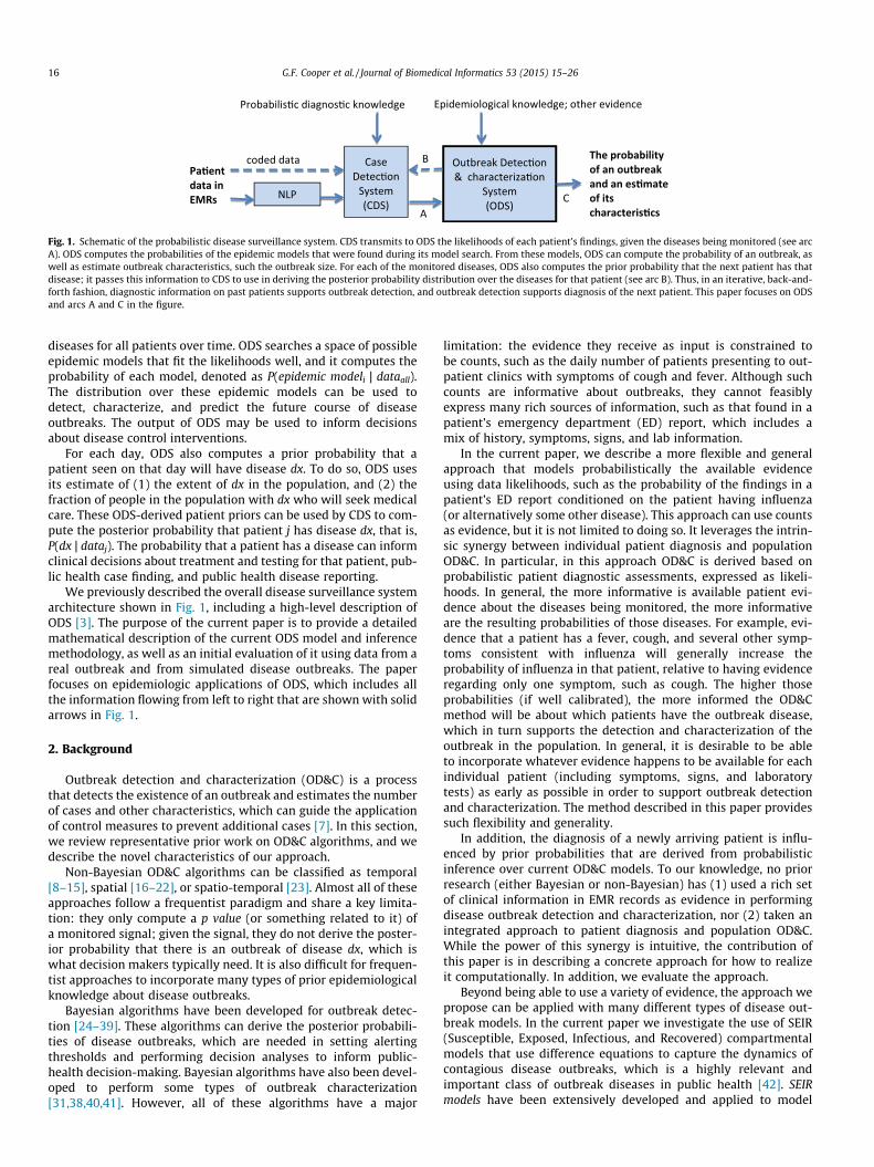
ness and forecasting of the future course of epidemics. As depictedin Fig. 1, the framework supports disease surveillance end-to-end,from patient data to outbreak detection and characterization.Moreover, since detection and characterization are probabilistic,they can serve as input to a decision-theoretic decision-supportsystem that aids public-health decision making about disease-con-trol interventions, as we describe in [3].

In the approach, a case detection system (CDS) obtains patientdata (evidence) from electronic medical records (EMRs) [4]. Thepatient data include symptoms and signs extracted by a naturallanguage processing (NLP) system from text reports. CDS uses dataabout the patient and probabilistic diagnostic knowledge in theform of Bayesian networks [5] to infer a probability distributionover the diseases that a patient may have. For a given patient-casej, the result of this inference is expressed as likelihoods of thepatient’s data Ej, both with and without an outbreak disease dx.In a recently reported study, CDS achieved an area under theROC curve of 0.75 (95% CI: 0.69 to 0.82) in identifying influenzacases from findings in ED reports [6].

A second component of the system, which is the focus of thispaper, is the outbreak detection and characterization system(ODS). ODS receives from CDS the likelihoods of monitored

Pa�entdata in EMRs

Outbreak Detec�on & characteriza�on

System (ODS)

Epidemiological knowledge; other evidence

Case Detec�on

System(CDS)

Probabilis�c diagnos�c knowledge

NLP

coded data B

A

The probability of an outbreak and an es�mateof its characteris�cs

C

Fig. 1. Schematic of the probabilistic disease surveillance system. CDS transmits to ODS the likelihoods of each patient’s findings, given the diseases being monitored (see arcA). ODS computes the probabilities of the epidemic models that were found during its model search. From these models, ODS can compute the probability of an outbreak, aswell as estimate outbreak characteristics, such the outbreak size. For each of the monitored diseases, ODS also computes the prior probability that the next patient has thatdisease; it passes this information to CDS to use in deriving the posterior probability distribution over the diseases for that patient (see arc B). Thus, in an iterative, back-and-forth fashion, diagnostic information on past patients supports outbreak detection, and outbreak detection supports diagnosis of the next patient. This paper focuses on ODSand arcs A and C in the figure.

16 G.F. Cooper et al. / Journal of Biomedical Informatics 53 (2015) 15–26

diseases for all patients over time. ODS searches a space of possibleepidemic models that fit the likelihoods well, and it computes theprobability of each model, denoted as P(epidemic modeli | dataall).The distribution over these epidemic models can be used todetect, characterize, and predict the future course of diseaseoutbreaks. The output of ODS may be used to inform decisionsabout disease control interventions.

For each day, ODS also computes a prior probability that apatient seen on that day will have disease dx. To do so, ODS usesits estimate of (1) the extent of dx in the population, and (2) thefraction of people in the population with dx who will seek medicalcare. These ODS-derived patient priors can be used by CDS to com-pute the posterior probability that patient j has disease dx, that is,P(dx | dataj). The probability that a patient has a disease can informclinical decisions about treatment and testing for that patient, pub-lic health case finding, and public health disease reporting.

We previously described the overall disease surveillance systemarchitecture shown in Fig. 1, including a high-level description ofODS [3]. The purpose of the current paper is to provide a detailedmathematical description of the current ODS model and inferencemethodology, as well as an initial evaluation of it using data from areal outbreak and from simulated disease outbreaks. The paperfocuses on epidemiologic applications of ODS, which includes allthe information flowing from left to right that are shown with solidarrows in Fig. 1.

2. Background

Outbreak detection and characterization (OD&C) is a processthat detects the existence of an outbreak and estimates the numberof cases and other characteristics, which can guide the applicationof control measures to prevent additional cases [7]. In this section,we review representative prior work on OD&C algorithms, and wedescribe the novel characteristics of our approach.

Non-Bayesian OD&C algorithms can be classified as temporal[8–15], spatial [16–22], or spatio-temporal [23]. Almost all of theseapproaches follow a frequentist paradigm and share a key limita-tion: they only compute a p value (or something related to it) ofa monitored signal; given the signal, they do not derive the poster-ior probability that there is an outbreak of disease dx, which iswhat decision makers typically need. It is also difficult for frequen-tist approaches to incorporate many types of prior epidemiologicalknowledge about disease outbreaks.

Bayesian algorithms have been developed for outbreak detec-tion [24–39]. These algorithms can derive the posterior probabili-ties of disease outbreaks, which are needed in setting alertingthresholds and performing decision analyses to inform public-health decision-making. Bayesian algorithms have also been devel-oped to perform some types of outbreak characterization[31,38,40,41]. However, all of these algorithms have a major

limitation: the evidence they receive as input is constrained tobe counts, such as the daily number of patients presenting to out-patient clinics with symptoms of cough and fever. Although suchcounts are informative about outbreaks, they cannot feasiblyexpress many rich sources of information, such as that found in apatient’s emergency department (ED) report, which includes amix of history, symptoms, signs, and lab information.

In the current paper, we describe a more flexible and generalapproach that models probabilistically the available evidenceusing data likelihoods, such as the probability of the findings in apatient’s ED report conditioned on the patient having influenza(or alternatively some other disease). This approach can use countsas evidence, but it is not limited to doing so. It leverages the intrin-sic synergy between individual patient diagnosis and populationOD&C. In particular, in this approach OD&C is derived based onprobabilistic patient diagnostic assessments, expressed as likeli-hoods. In general, the more informative is available patient evi-dence about the diseases being monitored, the more informativeare the resulting probabilities of those diseases. For example, evi-dence that a patient has a fever, cough, and several other symp-toms consistent with influenza will generally increase theprobability of influenza in that patient, relative to having evidenceregarding only one symptom, such as cough. The higher thoseprobabilities (if well calibrated), the more informed the OD&Cmethod will be about which patients have the outbreak disease,which in turn supports the detection and characterization of theoutbreak in the population. In general, it is desirable to be ableto incorporate whatever evidence happens to be available for eachindividual patient (including symptoms, signs, and laboratorytests) as early as possible in order to support outbreak detectionand characterization. The method described in this paper providessuch flexibility and generality.

In addition, the diagnosis of a newly arriving patient is influ-enced by prior probabilities that are derived from probabilisticinference over current OD&C models. To our knowledge, no priorresearch (either Bayesian or non-Bayesian) has (1) used a rich setof clinical information in EMR records as evidence in performingdisease outbreak detection and characterization, nor (2) taken anintegrated approach to patient diagnosis and population OD&C.While the power of this synergy is intuitive, the contribution ofthis paper is in describing a concrete approach for how to realizeit computationally. In addition, we evaluate the approach.

Beyond being able to use a variety of evidence, the approach wepropose can be applied with many different types of disease out-break models. In the current paper we investigate the use of SEIR(Susceptible, Exposed, Infectious, and Recovered) compartmentalmodels that use difference equations to capture the dynamics ofcontagious disease outbreaks, which is a highly relevant andimportant class of outbreak diseases in public health [42]. SEIRmodels have been extensively developed and applied to model

G.F. Cooper et al. / Journal of Biomedical Informatics 53 (2015) 15–26 17

contagious disease outbreaks [42]. In particular, this paper focuseson modeling influenza using a SEIR model, which is an importantclass of pathogens that cause disease outbreaks and pandemics.

3. Computational methods

This section first describes the general approach we have devel-oped for deriving the posterior probabilities of epidemic models foruse in detecting and characterizing a disease outbreak. It then givesa general description of a method for searching over models.

3.1. Model scoring

Our goal is to take clinical evidence in the form of EMR data,such as real-time ED reports, and to then automatically inferwhether a disease outbreak is occurring in the population at large,and if so, its characteristics. Let dataall represent all of the availablepatient data and let modeli denote a specific model (epidemiologi-cal hypothesis) of the disease outbreak in the population. By Bayes’theorem we obtain the following:

Pðmodeli j dataallÞ ¼Pðdataall;modeliÞ

PðdataallÞ

¼ Pðdataall jmodeliÞ � PðmodeliÞPmodeli2SPðdataall jmodeliÞ � PðmodeliÞ

; ð1Þ

where the sum is taken over all the models in set S that we assumehave a non-zero prior probability (i.e., P(modeli) > 0).

In Eq. (1), P(modeli) is the prior probability of modeli, which isassessed based on domain knowledge about possible types of out-breaks and their characteristics. For example, if we are using SEIRmodels [42,43], then the basic reproduction number R0 is one suchcharacteristic of population disease. By convention, we considermodel0 to be a model that represents the absence of a diseaseoutbreak.

We derive P(dataall | modeli) in Eq. (1) as follows. Given a model,we assume that the evidence over all patients on each given day,1

which we denote as E(day), is conditionally independent of evidenceon other days, given a model:

Pðdataall jmodeliÞ ¼YEndDay

day¼StartDay

PðEðdayÞ jmodeliÞ; ð2Þ

where the product is over all the days that we are monitoring for anoutbreak, from an initial StartDay to a final EndDay, which typicallywould be the most recent day for which we have data, such as EMRdata. We emphasize that in general modeli is a temporal, diseasetransmission model, which represents that the evidence on oneday is related to the evidence of another day; so, the evidence fromone day to the next is not unconditionally independent; rather, inEq. (2) the evidence is only assumed to be independent givenmodeli.

Let r be the number of patients (e.g., ED patients) on a given daywho have the outbreak disease dx (e.g., influenza) that is beingmonitored.2 As we will see below, it is convenient to average overall values of r to derive the term in the product of Eq. (2) as follows:

PðEðdayÞ jmodeliÞ ¼X#PtsðdayÞ

r¼0

PðEðdayÞ j r;modeliÞ � Pðr jmodeliÞ; ð3Þ

where #Pts(day) is a function that returns the total number ofpatients who visited the health facilities being monitored on a givenday.

1 The unit of time need not be days, but rather could be hours, for example.2 For simplicity of presentation we assume here that only one disease is being

monitored for an outbreak.

We derive the first term in the sum of Eq. (3) as follows. The evi-dence for each day consists of the evidence over all of the patientsseen on that day. We denote the evidence for an arbitrary patient jas Ej(day | r, modeli); for example, it might consist of all the findingsfor the patient on that day that are recorded in an EMR by a phy-sician. We assume that the evidence of one patient is conditionallyindependent of the evidence of another patient, given a model anda value for r. Thus, we have the following:

PðEðdayÞ j r;modeliÞ ¼Y#PtsðdayÞ

j¼1

PðEjðdayÞ j r;modeliÞ; ð4Þ

Let dx = 1 represent that patient j has the outbreak disease dx, andlet dx = 0 represent that he or she does not. Conditioned on knowingthe disease status of a patient, we assume that the evidence aboutthat patient’s disease status is independent of r and modeli. Underthis assumption, the term in the product of Eq. (4) is as follows:

PðEjðdayÞ j r;modeliÞ¼ PðEjðdayÞ jdx¼1Þ �Pðdx¼1 j r;modeliÞþPðEjðdayÞ jdx¼0Þ �Pðdx¼0 j r;modeliÞ: ð5Þ

Recall that modeli is a model of the outbreak disease dx in the pop-ulation at large, r is the number of presenting patients on a givenday that have disease dx, and P(dx = 1 | r, modeli) is the prior proba-bility that a given patient will have dx given r and modeli. Clearlythis probability is influenced by the value of r; however, given r,knowing modeli would generally provide no additional informationabout the chance that the patient has disease dx. Based on this lineof reasoning, we obtain the following:

Pðdx ¼ 1 j r;modeliÞ ¼ Pðdx ¼ 1 j rÞ; and ð6aÞ

Pðdx ¼ 0 j r;modeliÞ ¼ Pðdx ¼ 0 j rÞ: ð6bÞ

Substituting Eqs. (6a) and (6b) into Eq. (5), we obtain the following:

PðEjðdayÞ j r;modeliÞ ¼ PðEjðdayÞ j dx ¼ 1Þ � Pðdx ¼ 1 j rÞþ PðEjðdayÞ j dx ¼ 0Þ � Pðdx ¼ 0 j rÞ: ð7Þ

For a given value of r, we derive the prior probability that a patienthas disease dx as follows:

Pðdx ¼ 1 j rÞ ¼ r#PtsðdayÞ ;

where recall that #Pts(day) is the total number of patients on thatday who sought care, which is a known quantity. We also have thatP(dx = 0 | r) = 1 – P(dx = 1 | r).

The likelihood terms P(Ej(day) | dx = 1) and P(Ej(day) | dx = 0) inEq. (7) are provided by CDS, which is described in detail in [4]. Inthis way, CDS passes patient-centric information to ODS for it touse in performing disease detection and characterization. Animportant point to emphasize is that Ej can represent an arbitrarilyrich and diverse set of patient information; in the limit, it could rep-resent everything that is known about the patient at the time thatcare is sought. This point highlights the generality of the approachbeing described here in terms of linking the clinical care of individ-ual patients to the epidemiological assessment of disease in thepopulation.

We now return to Eq. (3) to derive P(r | modeli), which will com-plete the analysis. Let n represent the number of individuals whoaccording to modeli are infected with a given pathogen that is caus-ing dx in the population on a particular day and are subject to vis-iting the ED because of their infection. Let h denote the probabilitythat a person in the population with dx will seek care and therebybecome a patient who is seen on the given day. Assuming thesepatients seek care independently of each other, we obtain thefollowing:

Pðr jmodeliÞ ¼ Binomialðr; n; hÞ; ð8Þ

18 G.F. Cooper et al. / Journal of Biomedical Informatics 53 (2015) 15–26

where Binomial(r; n, h) denotes a binomial distribution over r, givenvalues of n and h. If r > n, then Binomial(r; n, h) = 0.

Eq. (8) assumes that n and h are known with certainty; however,in general they are not. By considering the distribution of the val-ues of n, we generalize Eq. (8) to be the following:

Pðr jmodeliÞ ¼XNpop

n¼0

Binomialðr; n; hÞ � Pðn jmodeliÞ; ð9Þ

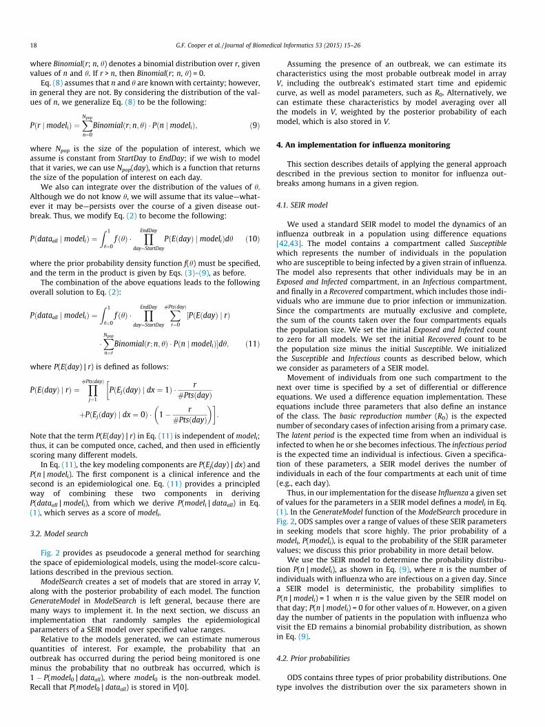
where Npop is the size of the population of interest, which weassume is constant from StartDay to EndDay; if we wish to modelthat it varies, we can use Npop(day), which is a function that returnsthe size of the population of interest on each day.

We also can integrate over the distribution of the values of h.Although we do not know h, we will assume that its value—what-ever it may be—persists over the course of a given disease out-break. Thus, we modify Eq. (2) to become the following:

Pðdataall jmodeliÞ ¼Z 1

h¼0f ðhÞ �

YEndDay

day¼StartDay

PðEðdayÞ jmodeliÞdh ð10Þ

where the prior probability density function f(h) must be specified,and the term in the product is given by Eqs. (3)–(9), as before.

The combination of the above equations leads to the followingoverall solution to Eq. (2):

Pðdataall jmodeliÞ ¼Z 1

h¼0f ðhÞ �

YEndDay

day¼StartDay

X#PtsðdayÞ

r¼0

½PðEðdayÞ j rÞ

�XNpop

n¼r

Binomialðr; n; hÞ � Pðn jmodeliÞ�dh; ð11Þ

where P(E(day) | r) is defined as follows:

PðEðdayÞ j rÞ ¼Y#PtsðdayÞ

j¼1

PðEjðdayÞ j dx ¼ 1Þ � r#PtsðdayÞ

�

þPðEjðdayÞ j dx ¼ 0Þ � 1� r#PtsðdayÞ

� ��:

Note that the term P(E(day) | r) in Eq. (11) is independent of modeli;thus, it can be computed once, cached, and then used in efficientlyscoring many different models.

In Eq. (11), the key modeling components are P(Ej(day) | dx) andP(n | modeli). The first component is a clinical inference and thesecond is an epidemiological one. Eq. (11) provides a principledway of combining these two components in derivingP(dataall | modeli), from which we derive P(modeli | dataall) in Eq.(1), which serves as a score of modeli.

3.2. Model search

Fig. 2 provides as pseudocode a general method for searchingthe space of epidemiological models, using the model-score calcu-lations described in the previous section.

ModelSearch creates a set of models that are stored in array V,along with the posterior probability of each model. The functionGenerateModel in ModelSearch is left general, because there aremany ways to implement it. In the next section, we discuss animplementation that randomly samples the epidemiologicalparameters of a SEIR model over specified value ranges.

Relative to the models generated, we can estimate numerousquantities of interest. For example, the probability that anoutbreak has occurred during the period being monitored is oneminus the probability that no outbreak has occurred, which is1 � P(model0 | dataall), where model0 is the non-outbreak model.Recall that P(model0 | dataall) is stored in V[0].

Assuming the presence of an outbreak, we can estimate itscharacteristics using the most probable outbreak model in arrayV, including the outbreak’s estimated start time and epidemiccurve, as well as model parameters, such as R0. Alternatively, wecan estimate these characteristics by model averaging over allthe models in V, weighted by the posterior probability of eachmodel, which is also stored in V.

4. An implementation for influenza monitoring

This section describes details of applying the general approachdescribed in the previous section to monitor for influenza out-breaks among humans in a given region.

4.1. SEIR model

We used a standard SEIR model to model the dynamics of aninfluenza outbreak in a population using difference equations[42,43]. The model contains a compartment called Susceptiblewhich represents the number of individuals in the populationwho are susceptible to being infected by a given strain of influenza.The model also represents that other individuals may be in anExposed and Infected compartment, in an Infectious compartment,and finally in a Recovered compartment, which includes those indi-viduals who are immune due to prior infection or immunization.Since the compartments are mutually exclusive and complete,the sum of the counts taken over the four compartments equalsthe population size. We set the initial Exposed and Infected countto zero for all models. We set the initial Recovered count to bethe population size minus the initial Susceptible. We initializedthe Susceptible and Infectious counts as described below, whichwe consider as parameters of a SEIR model.

Movement of individuals from one such compartment to thenext over time is specified by a set of differential or differenceequations. We used a difference equation implementation. Theseequations include three parameters that also define an instanceof the class. The basic reproduction number (R0) is the expectednumber of secondary cases of infection arising from a primary case.The latent period is the expected time from when an individual isinfected to when he or she becomes infectious. The infectious periodis the expected time an individual is infectious. Given a specifica-tion of these parameters, a SEIR model derives the number ofindividuals in each of the four compartments at each unit of time(e.g., each day).

Thus, in our implementation for the disease Influenza a given setof values for the parameters in a SEIR model defines a modeli in Eq.(1). In the GenerateModel function of the ModelSearch procedure inFig. 2, ODS samples over a range of values of these SEIR parametersin seeking models that score highly. The prior probability of amodeli, P(modeli), is equal to the probability of the SEIR parametervalues; we discuss this prior probability in more detail below.

We use the SEIR model to determine the probability distribu-tion P(n | modeli), as shown in Eq. (9), where n is the number ofindividuals with influenza who are infectious on a given day. Sincea SEIR model is deterministic, the probability simplifies toP(n | modeli) = 1 when n is the value given by the SEIR model onthat day; P(n | modeli) = 0 for other values of n. However, on a givenday the number of patients in the population with influenza whovisit the ED remains a binomial probability distribution, as shownin Eq. (9).

4.2. Prior probabilities

ODS contains three types of prior probability distributions. Onetype involves the distribution over the six parameters shown in

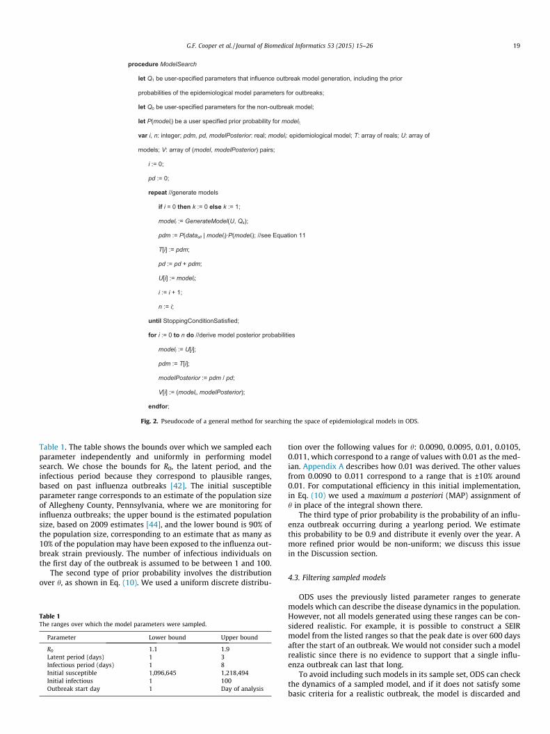
Fig. 2. Pseudocode of a general method for searching the space of epidemiological models in ODS.

G.F. Cooper et al. / Journal of Biomedical Informatics 53 (2015) 15–26 19

Table 1. The table shows the bounds over which we sampled eachparameter independently and uniformly in performing modelsearch. We chose the bounds for R0, the latent period, and theinfectious period because they correspond to plausible ranges,based on past influenza outbreaks [42]. The initial susceptibleparameter range corresponds to an estimate of the population sizeof Allegheny County, Pennsylvania, where we are monitoring forinfluenza outbreaks; the upper bound is the estimated populationsize, based on 2009 estimates [44], and the lower bound is 90% ofthe population size, corresponding to an estimate that as many as10% of the population may have been exposed to the influenza out-break strain previously. The number of infectious individuals onthe first day of the outbreak is assumed to be between 1 and 100.

The second type of prior probability involves the distributionover h, as shown in Eq. (10). We used a uniform discrete distribu-

Table 1The ranges over which the model parameters were sampled.

Parameter Lower bound Upper bound

R0 1.1 1.9Latent period (days) 1 3Infectious period (days) 1 8Initial susceptible 1,096,645 1,218,494Initial infectious 1 100Outbreak start day 1 Day of analysis

tion over the following values for h: 0.0090, 0.0095, 0.01, 0.0105,0.011, which correspond to a range of values with 0.01 as the med-ian. Appendix A describes how 0.01 was derived. The other valuesfrom 0.0090 to 0.011 correspond to a range that is ±10% around0.01. For computational efficiency in this initial implementation,in Eq. (10) we used a maximum a posteriori (MAP) assignment ofh in place of the integral shown there.

The third type of prior probability is the probability of an influ-enza outbreak occurring during a yearlong period. We estimatethis probability to be 0.9 and distribute it evenly over the year. Amore refined prior would be non-uniform; we discuss this issuein the Discussion section.

4.3. Filtering sampled models

ODS uses the previously listed parameter ranges to generatemodels which can describe the disease dynamics in the population.However, not all models generated using these ranges can be con-sidered realistic. For example, it is possible to construct a SEIRmodel from the listed ranges so that the peak date is over 600 daysafter the start of an outbreak. We would not consider such a modelrealistic since there is no evidence to support that a single influ-enza outbreak can last that long.

To avoid including such models in its sample set, ODS can checkthe dynamics of a sampled model, and if it does not satisfy somebasic criteria for a realistic outbreak, the model is discarded and

20 G.F. Cooper et al. / Journal of Biomedical Informatics 53 (2015) 15–26

replaced with a new sample, which is checked in the same way. Forreal data, we assumed that a model is valid if its peak occurs withina 1-year period from the earliest possible start date of the out-break. For simulated data, we assumed a model is valid if it pre-dicts an outbreak to last no more than 240 days; the predictedoutbreak is defined to be over when the number of people pre-dicted to be infected is less than 1.

4.4. Modeling non-influenza influenza-like illness

An important task when monitoring for an influenza outbreak isto model patients who present to an ED showing symptoms consis-tent with influenza, but who do not actually have influenza. Suchpatients are described as exhibiting a non-influenza influenza-likeillness (NI-ILI). Cases of NI-ILI are frequent enough during both out-break and non-outbreak periods to form a baseline of influenza-likedisease. This baseline should be incorporated when applying themodeling approach described in Section 3 to detect and character-ize influenza outbreaks.

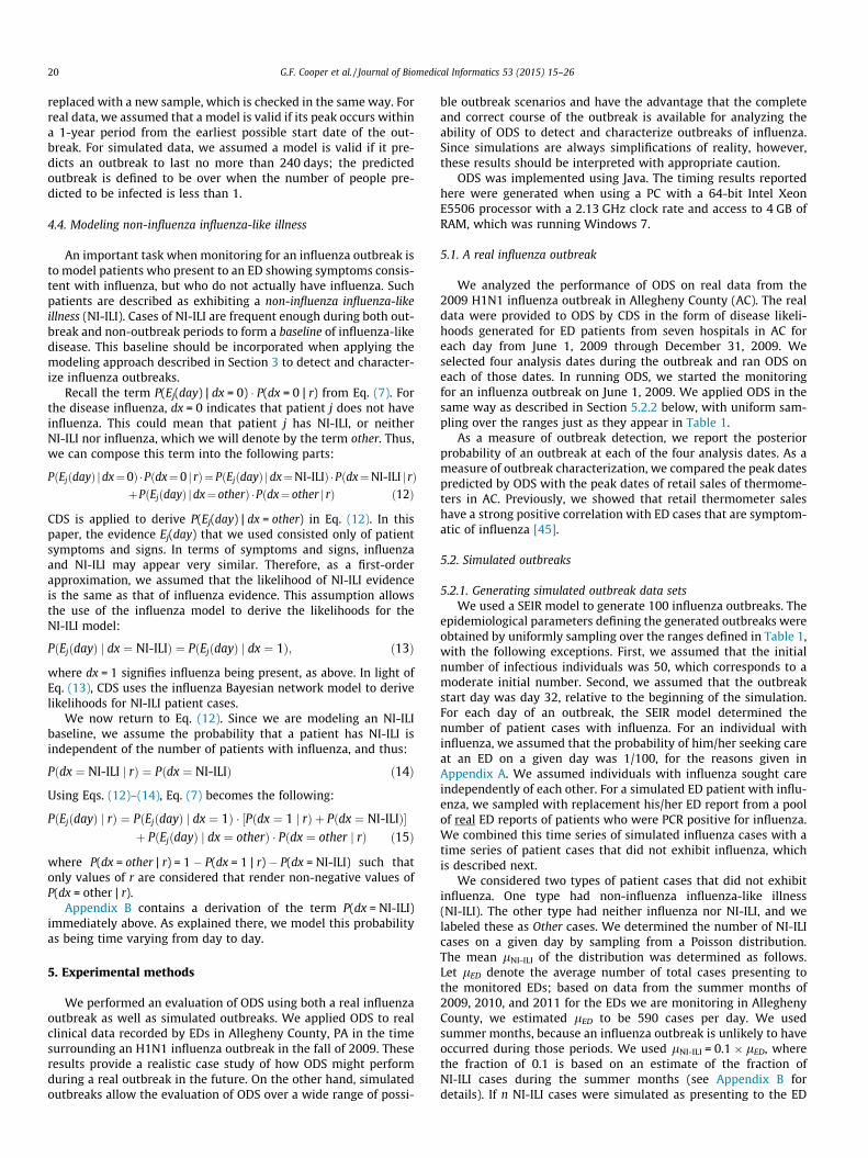
Recall the term P(Ej(day) | dx = 0) � P(dx = 0 | r) from Eq. (7). Forthe disease influenza, dx = 0 indicates that patient j does not haveinfluenza. This could mean that patient j has NI-ILI, or neitherNI-ILI nor influenza, which we will denote by the term other. Thus,we can compose this term into the following parts:

PðEjðdayÞ jdx¼0Þ �Pðdx¼0 j rÞ¼ PðEjðdayÞ jdx¼NI-ILIÞ �Pðdx¼NI-ILI j rÞþPðEjðdayÞ jdx¼ otherÞ �Pðdx¼ other j rÞ ð12Þ

CDS is applied to derive P(Ej(day) | dx = other) in Eq. (12). In thispaper, the evidence Ej(day) that we used consisted only of patientsymptoms and signs. In terms of symptoms and signs, influenzaand NI-ILI may appear very similar. Therefore, as a first-orderapproximation, we assumed that the likelihood of NI-ILI evidenceis the same as that of influenza evidence. This assumption allowsthe use of the influenza model to derive the likelihoods for theNI-ILI model:

PðEjðdayÞ j dx ¼ NI-ILIÞ ¼ PðEjðdayÞ j dx ¼ 1Þ; ð13Þ

where dx = 1 signifies influenza being present, as above. In light ofEq. (13), CDS uses the influenza Bayesian network model to derivelikelihoods for NI-ILI patient cases.

We now return to Eq. (12). Since we are modeling an NI-ILIbaseline, we assume the probability that a patient has NI-ILI isindependent of the number of patients with influenza, and thus:

Pðdx ¼ NI-ILI j rÞ ¼ Pðdx ¼ NI-ILIÞ ð14Þ

Using Eqs. (12)–(14), Eq. (7) becomes the following:

PðEjðdayÞ j rÞ ¼ PðEjðdayÞ j dx ¼ 1Þ � ½Pðdx ¼ 1 j rÞ þ Pðdx ¼ NI-ILIÞ�þ PðEjðdayÞ j dx ¼ otherÞ � Pðdx ¼ other j rÞ ð15Þ

where P(dx = other | r) = 1 � P(dx = 1 | r) � P(dx = NI-ILI) such thatonly values of r are considered that render non-negative values ofP(dx = other | r).

Appendix B contains a derivation of the term P(dx = NI-ILI)immediately above. As explained there, we model this probabilityas being time varying from day to day.

5. Experimental methods

We performed an evaluation of ODS using both a real influenzaoutbreak as well as simulated outbreaks. We applied ODS to realclinical data recorded by EDs in Allegheny County, PA in the timesurrounding an H1N1 influenza outbreak in the fall of 2009. Theseresults provide a realistic case study of how ODS might performduring a real outbreak in the future. On the other hand, simulatedoutbreaks allow the evaluation of ODS over a wide range of possi-

ble outbreak scenarios and have the advantage that the completeand correct course of the outbreak is available for analyzing theability of ODS to detect and characterize outbreaks of influenza.Since simulations are always simplifications of reality, however,these results should be interpreted with appropriate caution.

ODS was implemented using Java. The timing results reportedhere were generated when using a PC with a 64-bit Intel XeonE5506 processor with a 2.13 GHz clock rate and access to 4 GB ofRAM, which was running Windows 7.

5.1. A real influenza outbreak

We analyzed the performance of ODS on real data from the2009 H1N1 influenza outbreak in Allegheny County (AC). The realdata were provided to ODS by CDS in the form of disease likeli-hoods generated for ED patients from seven hospitals in AC foreach day from June 1, 2009 through December 31, 2009. Weselected four analysis dates during the outbreak and ran ODS oneach of those dates. In running ODS, we started the monitoringfor an influenza outbreak on June 1, 2009. We applied ODS in thesame way as described in Section 5.2.2 below, with uniform sam-pling over the ranges just as they appear in Table 1.

As a measure of outbreak detection, we report the posteriorprobability of an outbreak at each of the four analysis dates. As ameasure of outbreak characterization, we compared the peak datespredicted by ODS with the peak dates of retail sales of thermome-ters in AC. Previously, we showed that retail thermometer saleshave a strong positive correlation with ED cases that are symptom-atic of influenza [45].

5.2. Simulated outbreaks

5.2.1. Generating simulated outbreak data setsWe used a SEIR model to generate 100 influenza outbreaks. The

epidemiological parameters defining the generated outbreaks wereobtained by uniformly sampling over the ranges defined in Table 1,with the following exceptions. First, we assumed that the initialnumber of infectious individuals was 50, which corresponds to amoderate initial number. Second, we assumed that the outbreakstart day was day 32, relative to the beginning of the simulation.For each day of an outbreak, the SEIR model determined thenumber of patient cases with influenza. For an individual withinfluenza, we assumed that the probability of him/her seeking careat an ED on a given day was 1/100, for the reasons given inAppendix A. We assumed individuals with influenza sought careindependently of each other. For a simulated ED patient with influ-enza, we sampled with replacement his/her ED report from a poolof real ED reports of patients who were PCR positive for influenza.We combined this time series of simulated influenza cases with atime series of patient cases that did not exhibit influenza, whichis described next.

We considered two types of patient cases that did not exhibitinfluenza. One type had non-influenza influenza-like illness(NI-ILI). The other type had neither influenza nor NI-ILI, and welabeled these as Other cases. We determined the number of NI-ILIcases on a given day by sampling from a Poisson distribution.The mean lNI-ILI of the distribution was determined as follows.Let lED denote the average number of total cases presenting tothe monitored EDs; based on data from the summer months of2009, 2010, and 2011 for the EDs we are monitoring in AlleghenyCounty, we estimated lED to be 590 cases per day. We usedsummer months, because an influenza outbreak is unlikely to haveoccurred during those periods. We used lNI-ILI = 0.1 � lED, wherethe fraction of 0.1 is based on an estimate of the fraction ofNI-ILI cases during the summer months (see Appendix B fordetails). If n NI-ILI cases were simulated as presenting to the ED

G.F. Cooper et al. / Journal of Biomedical Informatics 53 (2015) 15–26 21

on a given day, we sampled with replacement n ED reports fromthe set of real influenza cases described above. Since in thisevaluation CDS used only symptoms and signs in the ED reportsto diagnosis influenza, we used influenza cases to represent thepresentation of other types of influenza-like illness.

We determined the number of Other cases on a given day bysampling from a Poisson distribution with a mean fraction of0.9 � lED. For each of these cases, we sampled an ED report froma pool of real ED reports of patients who (1) were negative forinfluenza according to a PCR test, or who did not have a PCR testordered, and (2) did not have symptoms consistent withinfluenza-like illness.

All cases were provided to CDS, which processed them and pro-vided likelihoods to ODS. For each day of a simulation, the simu-lated influenza patients who visited the ED were combined withthe simulated non-influenza patient cases who visited the ED(NI-ILI and Other cases) to create the set of all patients who visitedthe ED on that day. One hundred such simulated datasets weregenerated.

5.2.2. Applying ODS to the simulated outbreaksWe applied a version of ODS that implements the ModelSearch

algorithm in Fig. 2. ModelSearch sampled 10,000 SEIR models; thatis, once 10,000 SEIR models were sampled, the stopping conditionin the repeat statement of ModelSearch was satisfied. The Generate-Model function generated these SEIR models according to themethods described in Sections 4.1–4.3. In particular, in generatinga SEIR model the parameters in Table 1 were uniformly randomlysampled over the ranges shown there and then filtered to retainrealistic models.

We performed Bayesian model averaging over the 10,000 SEIRmodels to predict the total size of the outbreak for each of the100 simulated outbreaks. Thus, the prediction of outbreak sizefrom each model was weighed by the posterior probability of thatmodel, which was normalized so that the sum of the posteriorprobabilities over all 10,000 models summed to 1. To predict thepeak date, we derived a model averaged daily influenza incidencecurve, by Bayesian model averaging over the 10,000 influenzaincidence curves. We then identified the peak date in the modelaveraged curve and used it as the predicted peak date.

5.2.3. Analyzing ODS performance on simulated outbreaksWe quantified outbreak progression as being the fraction at

some point of the total number of outbreak cases that occurred overthe entire course of the outbreak. For example, 0.5 corresponds tohalf of the total cases having had occurred. We also derived thecorresponding number of days into the outbreak.

We analyzed the ability of ODS to detect and characterize out-breaks. We analyzed the posterior probability that an outbreak isoccurring on a given date, as computed by ODS, in order to assessthe timeliness of detection. An outbreak probability is only usefulif it is high when an outbreak is occurring and low when an out-break is not occurring. Thus, for a given outbreak posterior proba-bility P, we also report an estimate of the fraction of days during anon-outbreak period when ODS would predict an outbreak proba-bility as being greater than or equal to P. We assume that outbreakprobabilities from ODS are being generated on a daily basis.

We used two measures of population-wide outbreak character-ization performance. First, we measured how well ODS estimatedthe total number of outbreak cases (including future cases) as theoutbreak progressed. As a quantitative measure, we used |actual_number – estimated_number | /actual_number, which isthe relative error (RE). Second, we measured how well ODSestimated the peak day of an outbreak, using | actual_peak_date –estimated_peak_date |, which is the absolute error that ismeasured in days.

6. Experimental results

6.1. Results using real data

On August 15, 2009 the posterior probability of an influenzaoutbreak according to ODS was about 26%, which is moderate,but certainly not definitive. By September 8 the probability hadrisen to about 97%, which is 41 days before the October 19 peakdate of the outbreak, as discussed below. Table 2 shows the poster-ior probabilities on September 8 and three subsequent dates in2009. The table also shows the predicted peak date of the outbreakaccording to ODS and the peak date according to thermometersales.

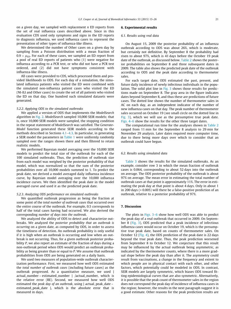
For each target date, ODS estimated the past, present, andfuture daily incidence of newly infectious individuals in the popu-lation. The solid plot line in Fig. 3 shows those results for predic-tions made on September 8. The gray area in the figure indicatesdates beyond September 8, and thus these are predictions of futurecases. The dotted line shows the number of thermometer sales inAC on each day, as an independent indicator of the number ofnew influenza cases on that day. The peak number of thermometersales occurred on October 19 (see small circle on the dotted line inFig. 3), which we will use as the presumptive true peak date.Figs. 4–6 show the results for the other three target dates.

The computational run time for the analyses shown in Table 2ranged from 11 min for the September 8 analysis to 29 min forNovember 29 analysis. Later dates required more computer time,due to there being more days over which to consider that anoutbreak could have begun.

6.2. Results using simulated data

Table 3 shows the results for the simulated outbreaks. As anexample, consider row 3 in which the mean fraction of outbreakcases is 0.064, corresponding to about 52 days into the outbreakon average. The ODS posterior probability of the outbreak is about97% on average. The mean error in estimating the total number ofoutbreak cases at that point is approximately 11%. The error in esti-mating the peak day at that point is about 4 days. Only in about 1in 200 days (= 0.005) will there be a false-positive prediction of anoutbreak, relative to a posterior probability of 97%.

7. Discussion

The plots in Figs. 3–6 show how well ODS was able to predictthe peak day of a real outbreak that occurred in 2009. On Septem-ber 8 (Fig. 3), ODS predicted that a peak incidence of infectiousinfluenza cases would occur on October 19, which is the presump-tive true peak date, based on counts of thermometer sales. OnOctober 12 (Fig. 4), the ODS prediction of the peak date is 22 daysbeyond the true peak date. Thus, the peak prediction worsenedfrom September 8 to October 12. We conjecture that this resultmay be influenced by the actual outbreak being asymmetric, asindicated by the thermometer counts, where there is a more grad-ual slope before the peak day than after it. The asymmetry couldresult from vaccinations, a change in the frequency and extent towhich people are in physical contact with each other, and otherfactors, which potentially could be modeled in ODS. In contrast,SEIR models are largely symmetric, which biases ODS toward fit-ting epidemiological curves that are also symmetric. Alternatively,it is possible that the peak count of thermometer sales in the regiondoes not correspond the peak day of incidence of influenza cases inthe region; however, the results in the next paragraph suggest it isa good estimate. Other reasons for the peak prediction results are

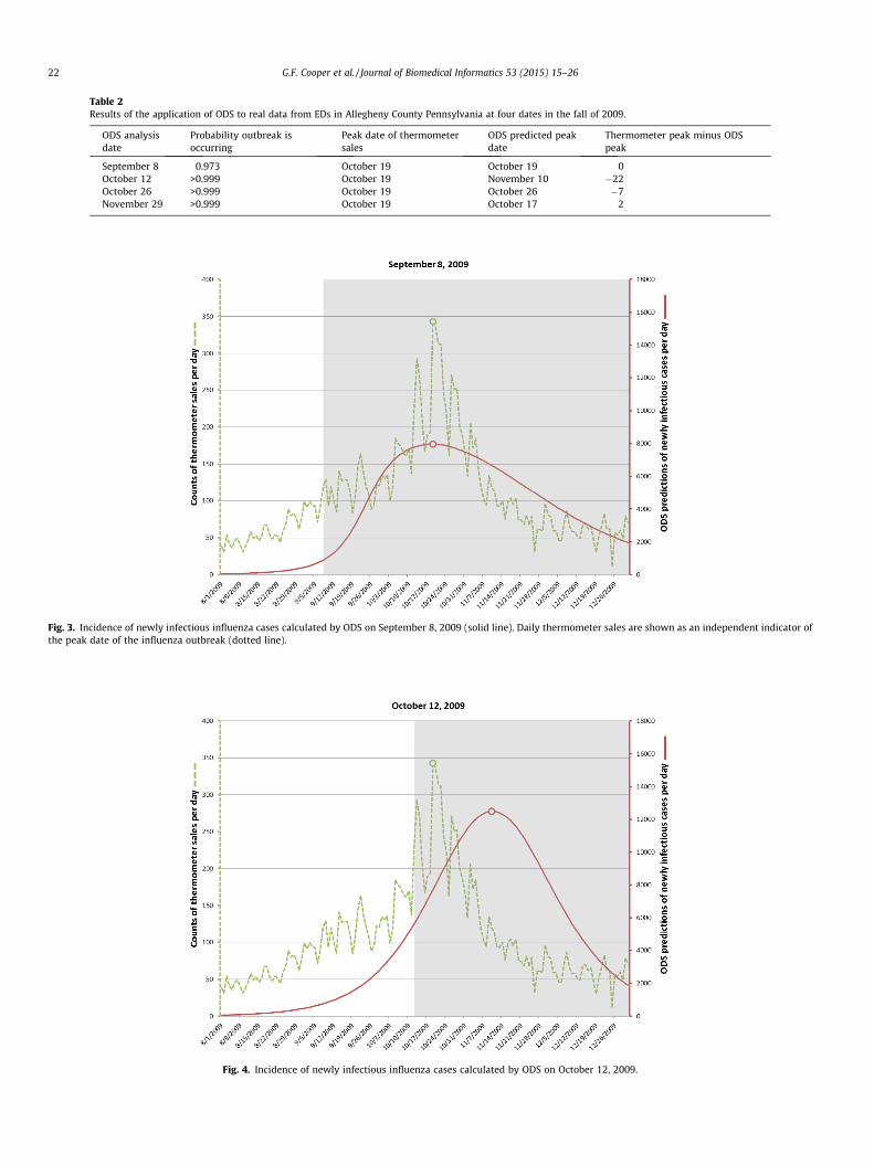
Table 2Results of the application of ODS to real data from EDs in Allegheny County Pennsylvania at four dates in the fall of 2009.

ODS analysisdate

Probability outbreak isoccurring

Peak date of thermometersales

ODS predicted peakdate

Thermometer peak minus ODSpeak

September 8 0.973 October 19 October 19 0October 12 >0.999 October 19 November 10 �22October 26 >0.999 October 19 October 26 �7November 29 >0.999 October 19 October 17 2

Fig. 3. Incidence of newly infectious influenza cases calculated by ODS on September 8, 2009 (solid line). Daily thermometer sales are shown as an independent indicator ofthe peak date of the influenza outbreak (dotted line).

Fig. 4. Incidence of newly infectious influenza cases calculated by ODS on October 12, 2009.

22 G.F. Cooper et al. / Journal of Biomedical Informatics 53 (2015) 15–26

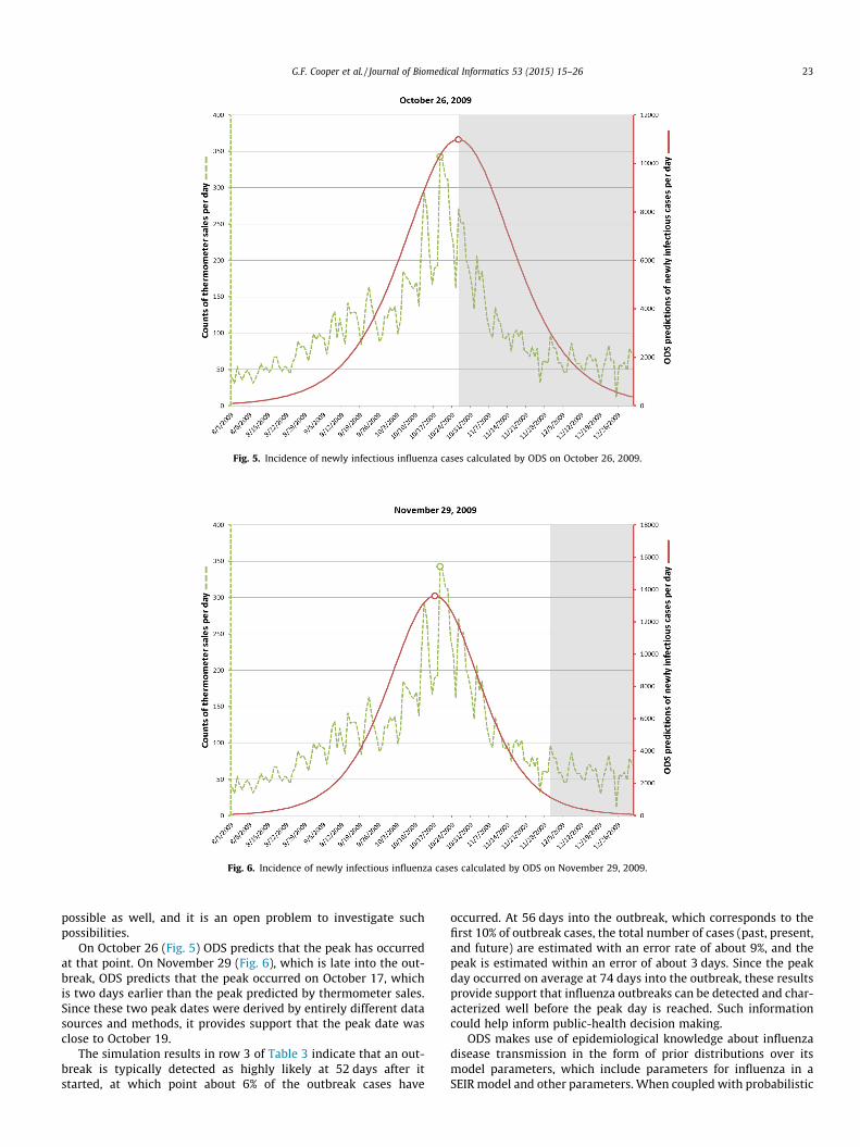
Fig. 5. Incidence of newly infectious influenza cases calculated by ODS on October 26, 2009.

Fig. 6. Incidence of newly infectious influenza cases calculated by ODS on November 29, 2009.

G.F. Cooper et al. / Journal of Biomedical Informatics 53 (2015) 15–26 23

possible as well, and it is an open problem to investigate suchpossibilities.

On October 26 (Fig. 5) ODS predicts that the peak has occurredat that point. On November 29 (Fig. 6), which is late into the out-break, ODS predicts that the peak occurred on October 17, whichis two days earlier than the peak predicted by thermometer sales.Since these two peak dates were derived by entirely different datasources and methods, it provides support that the peak date wasclose to October 19.

The simulation results in row 3 of Table 3 indicate that an out-break is typically detected as highly likely at 52 days after itstarted, at which point about 6% of the outbreak cases have

occurred. At 56 days into the outbreak, which corresponds to thefirst 10% of outbreak cases, the total number of cases (past, present,and future) are estimated with an error rate of about 9%, and thepeak is estimated within an error of about 3 days. Since the peakday occurred on average at 74 days into the outbreak, these resultsprovide support that influenza outbreaks can be detected and char-acterized well before the peak day is reached. Such informationcould help inform public-health decision making.

ODS makes use of epidemiological knowledge about influenzadisease transmission in the form of prior distributions over itsmodel parameters, which include parameters for influenza in aSEIR model and other parameters. When coupled with probabilistic

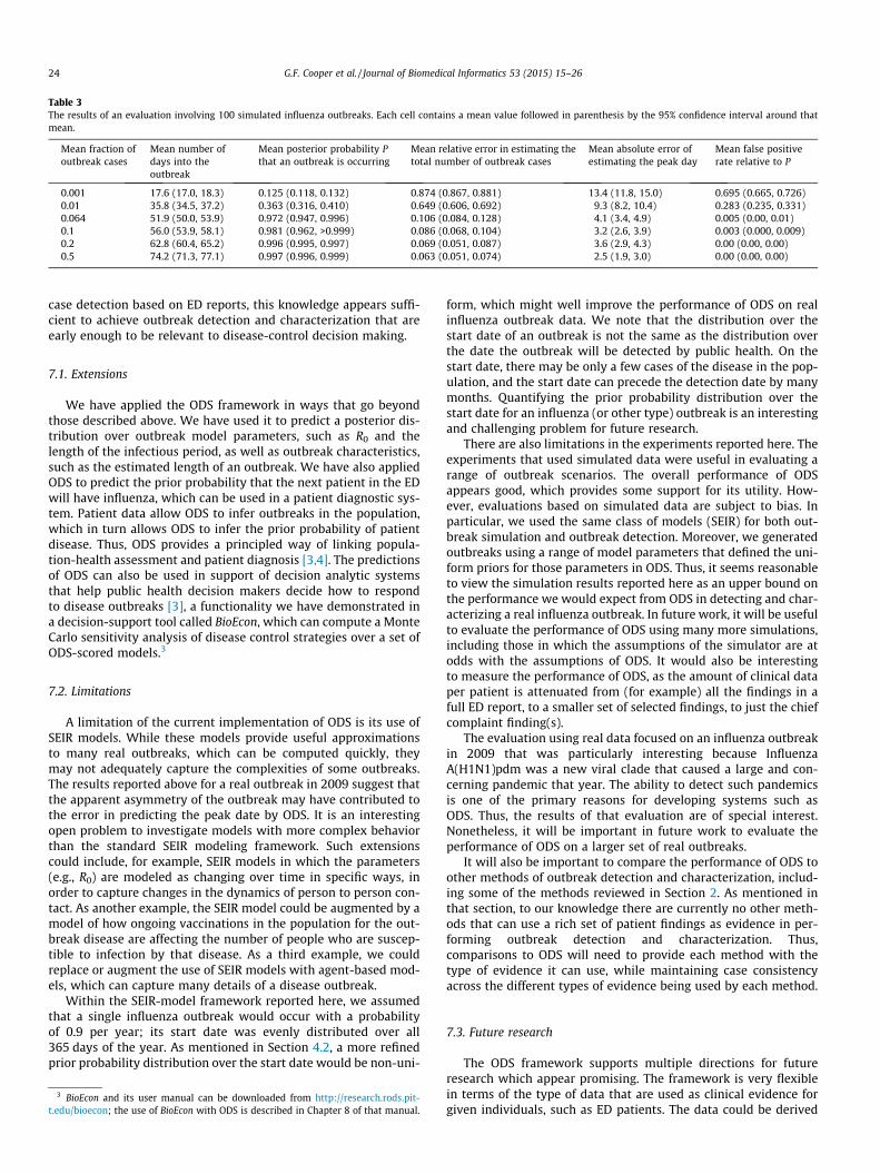
Table 3The results of an evaluation involving 100 simulated influenza outbreaks. Each cell contains a mean value followed in parenthesis by the 95% confidence interval around thatmean.

Mean fraction ofoutbreak cases

Mean number ofdays into theoutbreak

Mean posterior probability Pthat an outbreak is occurring

Mean relative error in estimating thetotal number of outbreak cases

Mean absolute error ofestimating the peak day

Mean false positiverate relative to P

0.001 17.6 (17.0, 18.3) 0.125 (0.118, 0.132) 0.874 (0.867, 0.881) 13.4 (11.8, 15.0) 0.695 (0.665, 0.726)0.01 35.8 (34.5, 37.2) 0.363 (0.316, 0.410) 0.649 (0.606, 0.692) 9.3 (8.2, 10.4) 0.283 (0.235, 0.331)0.064 51.9 (50.0, 53.9) 0.972 (0.947, 0.996) 0.106 (0.084, 0.128) 4.1 (3.4, 4.9) 0.005 (0.00, 0.01)0.1 56.0 (53.9, 58.1) 0.981 (0.962, >0.999) 0.086 (0.068, 0.104) 3.2 (2.6, 3.9) 0.003 (0.000, 0.009)0.2 62.8 (60.4, 65.2) 0.996 (0.995, 0.997) 0.069 (0.051, 0.087) 3.6 (2.9, 4.3) 0.00 (0.00, 0.00)0.5 74.2 (71.3, 77.1) 0.997 (0.996, 0.999) 0.063 (0.051, 0.074) 2.5 (1.9, 3.0) 0.00 (0.00, 0.00)

24 G.F. Cooper et al. / Journal of Biomedical Informatics 53 (2015) 15–26

case detection based on ED reports, this knowledge appears suffi-cient to achieve outbreak detection and characterization that areearly enough to be relevant to disease-control decision making.

7.1. Extensions

We have applied the ODS framework in ways that go beyondthose described above. We have used it to predict a posterior dis-tribution over outbreak model parameters, such as R0 and thelength of the infectious period, as well as outbreak characteristics,such as the estimated length of an outbreak. We have also appliedODS to predict the prior probability that the next patient in the EDwill have influenza, which can be used in a patient diagnostic sys-tem. Patient data allow ODS to infer outbreaks in the population,which in turn allows ODS to infer the prior probability of patientdisease. Thus, ODS provides a principled way of linking popula-tion-health assessment and patient diagnosis [3,4]. The predictionsof ODS can also be used in support of decision analytic systemsthat help public health decision makers decide how to respondto disease outbreaks [3], a functionality we have demonstrated ina decision-support tool called BioEcon, which can compute a MonteCarlo sensitivity analysis of disease control strategies over a set ofODS-scored models.3

7.2. Limitations

A limitation of the current implementation of ODS is its use ofSEIR models. While these models provide useful approximationsto many real outbreaks, which can be computed quickly, theymay not adequately capture the complexities of some outbreaks.The results reported above for a real outbreak in 2009 suggest thatthe apparent asymmetry of the outbreak may have contributed tothe error in predicting the peak date by ODS. It is an interestingopen problem to investigate models with more complex behaviorthan the standard SEIR modeling framework. Such extensionscould include, for example, SEIR models in which the parameters(e.g., R0) are modeled as changing over time in specific ways, inorder to capture changes in the dynamics of person to person con-tact. As another example, the SEIR model could be augmented by amodel of how ongoing vaccinations in the population for the out-break disease are affecting the number of people who are suscep-tible to infection by that disease. As a third example, we couldreplace or augment the use of SEIR models with agent-based mod-els, which can capture many details of a disease outbreak.

Within the SEIR-model framework reported here, we assumedthat a single influenza outbreak would occur with a probabilityof 0.9 per year; its start date was evenly distributed over all365 days of the year. As mentioned in Section 4.2, a more refinedprior probability distribution over the start date would be non-uni-

3 BioEcon and its user manual can be downloaded from http://research.rods.pit-t.edu/bioecon; the use of BioEcon with ODS is described in Chapter 8 of that manual.

form, which might well improve the performance of ODS on realinfluenza outbreak data. We note that the distribution over thestart date of an outbreak is not the same as the distribution overthe date the outbreak will be detected by public health. On thestart date, there may be only a few cases of the disease in the pop-ulation, and the start date can precede the detection date by manymonths. Quantifying the prior probability distribution over thestart date for an influenza (or other type) outbreak is an interestingand challenging problem for future research.

There are also limitations in the experiments reported here. Theexperiments that used simulated data were useful in evaluating arange of outbreak scenarios. The overall performance of ODSappears good, which provides some support for its utility. How-ever, evaluations based on simulated data are subject to bias. Inparticular, we used the same class of models (SEIR) for both out-break simulation and outbreak detection. Moreover, we generatedoutbreaks using a range of model parameters that defined the uni-form priors for those parameters in ODS. Thus, it seems reasonableto view the simulation results reported here as an upper bound onthe performance we would expect from ODS in detecting and char-acterizing a real influenza outbreak. In future work, it will be usefulto evaluate the performance of ODS using many more simulations,including those in which the assumptions of the simulator are atodds with the assumptions of ODS. It would also be interestingto measure the performance of ODS, as the amount of clinical dataper patient is attenuated from (for example) all the findings in afull ED report, to a smaller set of selected findings, to just the chiefcomplaint finding(s).

The evaluation using real data focused on an influenza outbreakin 2009 that was particularly interesting because InfluenzaA(H1N1)pdm was a new viral clade that caused a large and con-cerning pandemic that year. The ability to detect such pandemicsis one of the primary reasons for developing systems such asODS. Thus, the results of that evaluation are of special interest.Nonetheless, it will be important in future work to evaluate theperformance of ODS on a larger set of real outbreaks.

It will also be important to compare the performance of ODS toother methods of outbreak detection and characterization, includ-ing some of the methods reviewed in Section 2. As mentioned inthat section, to our knowledge there are currently no other meth-ods that can use a rich set of patient findings as evidence in per-forming outbreak detection and characterization. Thus,comparisons to ODS will need to provide each method with thetype of evidence it can use, while maintaining case consistencyacross the different types of evidence being used by each method.

7.3. Future research

The ODS framework supports multiple directions for futureresearch which appear promising. The framework is very flexiblein terms of the type of data that are used as clinical evidence forgiven individuals, such as ED patients. The data could be derived

G.F. Cooper et al. / Journal of Biomedical Informatics 53 (2015) 15–26 25

from free text using NLP, as reported here, as well as coded data,such as laboratory results. Moreover, the type of evidence availablefor one individual can be different from that available for another.For example, for some patients we may only know their chief com-plaint and basic demographic information. For others, we mayhave a rich set of clinical information for the EMR. The use ofheterogeneous data in outbreak detection and characterization isan open problem for future investigation.

The ODS framework is also flexible in supporting different typesof epidemiological models. For concreteness, in this paper we focuson using SEIR models; however, other epidemiological models canbe readily substituted. This paper also focuses on influenza as anexample of an outbreak disease. Nevertheless, influenza is not‘‘hard coded’’ into ODS. Rather, ODS allows other disease modelsto be used. It is possible for different types of outbreak diseasesto be modeled using different types of epidemiological models.For example, we could use a SEIR model for modeling influenzaand a SIS (Susceptible-Infectious-Susceptible) model for modelinggonorrhea.

ODS currently assumes at most one disease outbreak is influ-encing the data (during the interval from StartDay to EndDay).However, the general framework can accommodate the detectionof multiple outbreaks that are concurrent or sequential. An exam-ple is the detection of an RSV outbreak that begins and ends in themiddle of an influenza outbreak. Developing efficient computa-tional methods for detecting and characterizing multiple, overlap-ping outbreaks is an interesting area for future research.

An important problem is to detect and characterize an outbreakdisease that is an atypical variant of a known disease or is anunmodeled disease, perhaps due to it being novel. There are twomain patterns of evidence that can suggest the presence of suchevents. One occurs at the patient diagnosis level when modeleddiseases match patient findings relatively poorly for some patients.Another occurs at the epidemiological modeling level when theestimates of the epidemiological parameters for an ongoing out-break do not match well the parameter distributions of any ofthe currently modeled disease outbreaks. It is an interesting openproblem to develop a Bayesian method for combining these twosources of evidence to derive both (1) a posterior probability ofan outbreak being an atypical variant of some known disease and(2) a posterior probability that an outbreak is unmodeled, and thus,possibly novel.

Currently, ODS detects and characterizes outbreaks in a specificregion of interest, such as a county. It will be useful to extend it todetect and characterize outbreaks within subregions of a givenregion. Each subregion may have a different epidemiologicalbehavior (e.g., a different epidemiological curve in the case of anoutbreak of influenza) than the other subregions. Being able tocharacterize the individual and joint behavior of these subregionscould help support public health decision making.

As the capabilities of ODS are extended, it will be important tofurther improve its computational efficiency. One direction is touse more sophisticated methods to sample the model parameters,rather than use simple uniform sampling over a range of values.We could, for example, apply dynamic importance sampling [46],which tends to sample the parameters in the regions of the modelspace that appear to contain the most probable models. We mightalso assess more informative prior probability distributions overthe parameters.

8. Conclusions

This paper describes a novel Bayesian method called ODS forlinking epidemiological modeling and patient diagnosis to performdisease outbreak detection and characterization. The method was

applied to develop a system for detecting and characterizing influ-enza in a population from ED free-text reports. A SEIR model wasused to model influenza. A Bayesian belief network was used todevelop an influenza diagnostic system, which takes as evidencefindings that are extracted from ED reports using NLP methods.An evaluation was reported using simulated influenza data and areal outbreak of influenza in the Pittsburgh region in 2009. Theresults support the approach as promising in being able to detectoutbreaks well before the peak outbreak date, characterize whenthe peak will occur, and estimate the total size of the outbreak inthe case of simulated outbreaks. The general ODS framework isflexible and supports many directions for future extensions.

Acknowledgments

This research was supported by grant funding from the U.S.National Library of Medicine (R01-LM011370 and R01-LM009132), from the Center for Disease Control and Prevention(P01-HK000086), and from the U.S. National Science Foundation(IIS-0911032).

Appendix A.

This appendix describes the derivation of 1/100 as an estimateof the probability that an individual who is infectious with influ-enza on a given day of the outbreak will visit the ED on that daydue to the influenza. This posterior probability appears in Section4.2 of the paper. We factor it into the following four componentprobabilities:

Pðever infectious with influenza j infectious with influenza on day iÞ¼1:0 ðA1ÞPðever symptomatic with influenza jever infectious with influenzaÞ¼0:67 ðA2ÞPðever visit the ED with influenza j ever symptomatic with influenzaÞ¼0:09 ðA3ÞPðvisit ED on day i with influenza j ever visit the ED with influenzaÞ¼1=6 ðA4Þ

In the events appearing in the probabilities above, the word ‘‘ever’’refers to any time during a given individual’s infection with a givencase of influenza. Eq. (A1) is definitional. Eq. (A2) is based on assum-ing that only about 67% of individuals who become infected withinfluenza exhibit symptoms of influenza [47]. Eq. (A3) is based ona telephone survey performed in New York City in 2003, whichfound that about 9% of people who had symptoms of influenza saidthey visited an ED because of that episode of illness [48], (Table 2).Eq. (A4) assumes that if an individual will visit the ED due to symp-toms of influenza, then (1) the symptoms persist for an estimatedsix days [47], and (2) the individual is equally likely to visit theED on any one of those six days.The probability of interest is takento be the product of the above four probabilities:

Pðvisit ED on day i with influenza j infectious with influenza on day iÞ¼1�0:67�0:09�1=6�1=100:

Appendix B.

This appendix describes the method we applied to derive theprior probability of non-influenza influenza-like-illness (NI-ILI)on a given day. This quantity appears as P(dx = NI-ILI) in Eq. (15).A new value of this prior probability is derived for each day thatis being monitored for an outbreak.

Let d denote the variable day that appears in Eq. (15). It might,for example, denote the current day in a system that is monitoringfor outbreaks of disease. We would like to estimate the fraction Qof patient cases on day d that present for care due to having NI-ILI.We will then use fraction Q as our estimate of P(dx = NI-ILI) on day

26 G.F. Cooper et al. / Journal of Biomedical Informatics 53 (2015) 15–26

d. Let Qd be an estimate of Q on day d. Our goal is to estimate Qd

well.We first estimated values for Q during a period when we pre-

sume there is no outbreak of influenza. Since influenza outbreaksare unlikely in the summer, we used the summer months for thispurpose. For each day during the summer period, we found thevalue for the prior P(dx = NI-ILI) that maximized Eq. (3), assumingthat each patient case had either a NI-ILI or an Other disease. LetMLPd denote this maximum likelihood prior for day d. We thenderived the mean l and standard deviation r of these MLPd valuesover a period of summer days. Assuming a normal distribution, weused l and r to derive a threshold T such that only about 2.5% ofMLPd values are expected to be higher.

When monitoring for an outbreak on day d, we derived Qd asfollows. If MLPd�1 < T, then Qd := MLPd�1. The rationale is that anMLP value yesterday (d-1) that is below T is consistent with ILItoday (d) being due to non-influenza. However, if MLPd�1 P T thenan influenza outbreak is suspected, because it is unlikely that NI-ILIin the population could account for such a high extent of ILI. In thatcase, we estimate Qd as the mean value of recent, previous valuesof Q. In particular, we estimate Qd as being equal to the mean valueof Q over the previous 21 days prior to d; if fewer than 21 days areavailable, we use the number that is available; when d = 1, no pre-vious values are available, so we use Q1 = l. The rationale for usingthis method is that the current rate of NI-ILI is likely to be similarto its rate in the recent past.

References

[1] Obama B. National Strategy for Biosurveillance, Office of the President of theUnited States, Washington, DC; 2012. <http://www.whitehouse.gov/sites/default/files/National_Strategy_for_Biosurveillance_July_2012.pdf>.

[2] Ferguson NM, Cummings DA, Fraser C, Cajka JC, Cooley PC, Burke DS. Strategiesfor mitigating an influenza pandemic. Nature 2006;442(7101):448–52.

[3] Wagner MM, Tsui F, Cooper G, Espino JU, Levander J, Villamarin R, et al.Probabilistic, decision-theoretic disease surveillance and control. Online JPublic Health 2011;3(3).

[4] Tsui F, Wagner MM, Cooper G, Que J, Harkema H, Dowling J, et al. Probabilisticcase detection for disease surveillance using data in electronic medical records.Online J Public Health 2011;3(3).

[5] Darwiche A. Modeling and reasoning with Bayesian networks. CambridgeUniversity Press; 2009.

[6] Ye Y, Tsui F, Wagner M, Espino JU, Li Q. Influenza detection from emergencydepartment reports using natural language processing and Bayesian networkclassifiers. J Am Med Inform Assoc; 2014 [Published Online First].

[7] Wagner M. Chapter 1 Introduction. In: Wagner M, Moore A, Aryel R, editors.Handbook of Biosurveillance. New York: Elsevier; 2006.

[8] Page ES. Continuous inspection schemes. Biometrika 1954;41(1):100–15.[9] Serfling RE. Methods for current statistical analysis of excess pneumonia-

influenza deaths. Public Health Reports 1963;78(6):494–506.[10] Grant I. Recursive least squares. Teach Stat 1987;9(1):15–8.[11] Box GEP, Jenkins GM. Time series analysis: forecasting and control. Prentice

Hall; 1994.[12] Neubauer AS. The EWMA control chart: properties and comparison with other

quality-control procedures by computer simulation. Clin Chem1997;43(4):594–601.

[13] Zhang J, Tsui FC, Wagner MM, Hogan WR. Detection of outbreaks from timeseries data using a wavelet transform. In: Proceedings of the annual fallsymposium of the American medical informatics association; 2003.

[14] Ginsberg J, Mohebbi M, Patel R, Brammer L, Smolinski M, Brilliant L. Detectinginfluenza epidemics using search engine query data. Nature2009;457(7232):1012–4.

[15] Villamarin R, Cooper G, Tsui F-C, Wagner M, Espino J. Estimating the incidenceof influenza cases that present to emergency departments. In: Proceedings ofthe conference of the international society for disease surveillance; 2010.

[16] Kulldorff M. Spatial scan statistics: models, calculations, and applications. ScanStat Appl 1999:303–22.

[17] Kulldorff M. Prospective time periodic geographical disease surveillance usinga scan statistic. J Roy Stat Soc: Ser A (Stat Soc) 2001;164(1):61–72.

[18] Kleinman K, Lazarus R, Platt R. A generalized linear mixed models approach fordetecting incident clusters of disease in small areas, with an application tobiological terrorism. Am J Epidemiol 2004;159(3):217–24.

[19] Zeng D, Chang W, Chen H. A comparative study of spatio-temporal hotspotanalysis techniques in security informatics. In: Proceedings of theinternational IEEE conference on intelligent transportation systems. IEEE;2004. p. 106–111.

[20] Bradley CA, Rolka H, Walker D, Loonsk J. BioSense: implementation of anational early event detection and situational awareness system. MorbidMortal Weekly Rep (MMWR) 2005;54(Suppl):11–9.

[21] Duczmal L, Buckeridge D. Using modified spatial scan statistic to improvedetection of disease outbreak when exposure occurs in workplace – Virginia2004. Morbid Mortal Weekly Rep 2005;54(Supplement 187).

[22] Chang W, Zeng D, Chen H. Prospective spatio-temporal data analysis forsecurity informatics. In: Proceedings of the IEEE conference on intelligenttransportation systems. IEEE; 2005. p. 1120–24.

[23] Kulldorff M, Heffernan R, Hartman J, Assuncao R, Mostashari F. A space-timepermutation scan statistic for disease outbreak detection. PLoS Med2005;2(3):e59.

[24] Shiryaev AN. Optimal stopping rules. Springer; 1978.[25] Harvey AC. The Kalman filter and its applications in econometrics and time

series analysis. Methods Oper Res 1982;44(1):3–18.[26] Rabiner LR. A tutorial on hidden Markov models and selected applications in

speech recognition. Proc IEEE 1989;77(2):257–86.[27] Stroup DF, Thacker SB. A Bayesian approach to the detection of aberrations in

public health surveillance data. Epidemiology 1993;4(5):435–43.[28] Le Strat Y, Carrat F. Monitoring epidemiologic surveillance data using hidden

Markov models. Stat Med 1999;18(24):3463–78.[29] Nobre FF, Monteiro ABS, Telles PR, Williamson GD. Dynamic linear model and

SARIMA: a comparison of their forecasting performance in epidemiology. StatMed 2001;20(20):3051–69.

[30] Rath TM, Carreras M, Sebastiani P. Automated detection of influenza epidemicswith hidden Markov models. In: Proceedings of the international symposiumon intelligent data analysis; 2003.

[31] Jiang X, Wallstrom GL. A Bayesian network for outbreak detection andprediction. In: Proceedings of the conference of the American association forartificial intelligence; 2006. p. 1155–60.

[32] Neill DB, Moore AW, Cooper GF. A Bayesian spatial scan statistic. Adv NeurInform Process Syst 2006;18:1003–10.

[33] Sebastiani P, Mandl KD, Szolovits P, Kohane IS, Ramoni MF. A Bayesiandynamic model for influenza surveillance. Stat Med 2006;25(11):1803–16.

[34] Mnatsakanyan ZR, Burkom HS, Coberly JS, Lombardo JS. Bayesian informationfusion networks for biosurveillance applications. J Am Med Inform Assoc2009;16(6):855–63.

[35] Watkins R, Eagleson S, Veenendaal B, Wright G, Plant A. Disease surveillanceusing a hidden Markov model. BMC Med Inform Dec Making 2009;9(1):39.

[36] Chan T-C, King C-C, Yen M-Y, Chiang P-H, Huang C-S, Hsiao CK. Probabilisticdaily ILI syndromic surveillance with a spatio-temporal Bayesian hierarchicalmodel. PLoS ONE 2010;5(7):e11626.

[37] Neill DB, Cooper GF. A multivariate Bayesian scan statistic for early eventdetection and characterization. Mach Learn 2010;79(3):261–82.

[38] Ong JBS, Chen MIC, Cook AR, Lee HC, Lee VJ, Lin RTP, et al. Real-time epidemicmonitoring and forecasting of H1N1-2009 using influenza-like illness fromgeneral practice and family doctor clinics in Singapore. PLoS ONE2010;5(4):e10036.

[39] Burkom HS, Ramac-Thomas L, Babin S, Holtry R, Mnatsakanyan Z, Yund C. Anintegrated approach for fusion of environmental and human health data fordisease surveillance. Stat Med 2011;30(5):470–9.

[40] Skvortsov A, Ristic B, Woodruff C. Predicting an epidemic based on syndromicsurveillance. In: Proceedings of the conference on information fusion(FUSION); 2010. p. 1–8.

[41] Que J, Tsui FC. Spatial and temporal algorithm evaluation for detecting over-the-counter thermometer sales increasing during the 2009 H1N1 pandemic.Online J Public Health Inform 2012;4(1).

[42] Vynnycky E, White R. An introduction to infectious disease modelling. OxfordUniversity Press; 2010.

[43] Diekmann O, Heesterbeek JAP. Mathematical epidemiology of infectiousdiseases: model building, analysis, and interpretation. Wiley Chichester; 2000.

[44] Census US. Annual estimates of the resident population for counties ofPennsylvania; 2009. <http://www.census.gov/popest/data/counties/totals/2009/tables/CO-EST2009-01-42.csv>.

[45] Villamarin R, Cooper G, Wagner M, Tsui FC, Espino J. A method for estimatingfrom thermometer sales the incidence of diseases that are symptomaticallysimilar to influenza. J Biomed Inform 2013;46:444–57.

[46] Owen AB, Zhou Y. Safe and effective importance sampling. J Am Stat Assoc2000;95:135–43.

[47] Carrat F, Vergu E, Ferguson NM, Lemaitre M, Cauchemez S, Leach S, et al. Timelines of infection and disease in human influenza: a review of volunteerchallenge studies. Am J Epidemiol 2008;167:775–85.

[48] Metzger KB, Hajat A, Crawford M, Mostashari F. How many illnesses does oneemergency department visit represent? Using a population-based telephonesurvey to estimate the syndromic multiplier. Morbid Mortal Weekly Rep(MMWR) 2004;53(Syndromic Surveillance Supplement):106–11.