NASA Contractor Report 3207

Jet Transport Thunderstorm

Performance Wind Shear

:: ,

. In Conditions

John McCarthy, Edward F. Blick, and Randall R. Bensch

CONTRACT NASS-31377 DECEMBER 1979

II

https://ntrs.nasa.gov/search.jsp?R=19800005486 2020-04-26T22:16:56+00:00Z

TECH LIBRARY KAFB, NM

NASA Contractor Report 3207

Jet Transport Performance in Thunderstorm Wind Shear Conditions

John McCarthy, Edward F. Blick, and Randall R. Bensch The University of Oklahoma Nornzau, Oklahoma

Prepared for Marshall Space Flight Center under Contract NASS-3 1377

National Aeronautics and Space Administration

Scientific and Technical Information Branch

1979

I

I - -. -_

This document, prepared under the sponsorship of the National Aeronautics and Space Administration, is disseminated in the interest of information exchanges. It does not necessarily represent the views, technical approaches, or conclusions of NASA or any of its officials. The United States Government assumes no liability for its contents or the use thereof.

I

AUTHORS' ACKNOWLEDGEMENTS

The work reported herein was supported by the National

Aeronautics and Space Administration, Marshall Space Flight

Center, Space Sciences Laboratory, Atmospheric Sciences Di-

vision, under contract number NAS8-31377.

The authors wish to thank Mr. John H. Enders of the

Aviation Safety Technology Branch, Office of Aeronautics and

Space Technology (OAST), NASA Headquarters, Washington, D. C.,

for his support of this research. We greatly appreciate the

support of Mr. Dennis Camp, Of the Marshall Space Flight Cen-

ter, our project scientific monitor. Helpful discussions

with Dr. Walter Frost, of the University of Tennessee Space

Institute were important to this work.

The continuing support of the National Severe Storms

Laboratory, Norman, Oklahoma, was vital to this work. Spe-

cial thanks go to Dr. Edwin Kessler, Director, Dr. Richard

Doviak, Dr. Ron Alberty, Mr. Stephan Nelson, and Mr. Jean T.

Lee.

Aircraft data were provided by the Research Aviation

Facility, National Center for Atmospheric Research, @CAR),

funded by the National Science Foundation, to whom we are

grateful. The availability of NCAR aircraft data was due

to NSF support for basic thunderstorm research, under NSF

ATM74-0340ba02.

ii

I

TABLE OF CONTENTS

CHAPTER PAGE

I. INTRODUCTION . . . . ..I............................. 1

II. THE MODEL........................................ 4

1. The Equations of Motion ..................... 4 2. Bode Plots .................................. 6 3. Spectra of Wind Fields ...................... 17

III. AIRCRAFT APPROACH SIMULATIONS.................... 20

1. Theory ...................................... 20 2. Aircraft Simulations Using Real Data ........ 23 3. An Example: JFK Crash, 1975 ................ 35

IV. CONCLUSIONS...................................... 48

REFERENCES . . . . . . . . . . . . . . . . . . . . . . . . . . . . . . . . . . . . . . ..a.. 52

. . . 111

LIST OF FIGURES

FIGURE PAGE

1.

2.

3.

4.

5.

6.

7.

8.

9.

10.

11.

12.

Wind gust Bode plots for Boeing 727 class airplane . . . . . . . . . . . . . . . . . . . . . . . . . . . . . . . . . . . . . . . . .

Response of Boeing 727 class airplane to (a) half sine wave tailwind gust and (b) elevator step input during landing...............

Elevator angle Bode plots for Boeing 727 class airplane . . . . . . . . . . . . . . . . . . . . . . . . . . . . . . . . . . .

RMS altitude and velocity deviations of a Boeing 727 class airplane to continuous one m.sec -1 horizontal or vertical sine wave winds . . . . . . . . . . . . . . . . . . . . . . . . . . . . . . . . . . . . . . . . . . . .

RMS altitude and velocity deviations of a Boeing 727 class airplane to horizontal wind shears......................................

RMS altitude and velocity deviations of a Boeing 727 class airplane to vertical wind shears o........................... . . . . ..o...

Fixed-stick model simulation using NCAR aircraft data for 13 June 75 at 140230 CST................

Fixed-stick model simulation using NCAR aircraft data for 13 June 1975 at 142815 CST..........,...

The square of the least-squares correlation coefficient (variance explained) plotted against frequency, (a) for 13 June 75, and (b) for 19 May 77................................

Scattergrams relating Au' to ARWS function, expressed in dB, for (a) 13 June 75, and for (b) 19 May 77............-... . . . . . . . . . . . . . . . . . . . .

Sample simulation using KTVY tower data..........

Another KTVY tower sample simulation . . . . . . . . . . . . .

9

13

16

18

21

22

25

26

30

32

33

34

iv

r

FIGURE PAGE

13.

14.

15.

16.

17.

The square of the least-squares correlation coefficient (variance explained) plotted against frequency for eighty tower data simulations . . . . . . . . . ..a..........................

Scattergrams relating bu' to ARWS function, expressed in dB, for tower data..................

Longitudinal and vertical environment winds encountered by Eastern Flight 66.................

Model output for Eastern Flight 66 simulation......... . . . . . . . . . . . . . . . . . . . . . . . . . . . . . .

The estimated path of Eastern Flight 66, after Fujita and Caracena (1977).................

36

37

40

41

47

V

I..

cD

cL

h

hn

Ah'

IAS

I Y.Y

q

u,w

Au'

5 Xu’XwJg

zu,zw,z;,zq,z 6

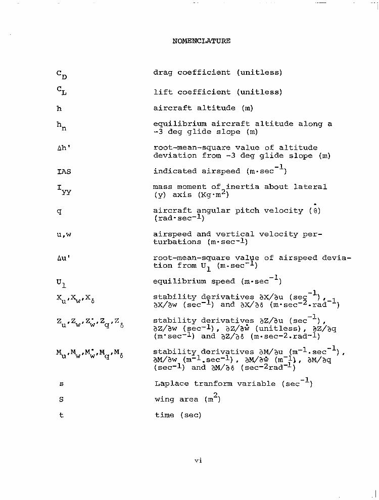
NOMENCLATURE:

drag coefficient (unitless)

lift coefficient (unitless)

aircraft altitude (m)

equilibrium aircraft altitude along a -3 deg glide slope (m)

root-mean-square value of altitude deviation from -3 deg glide slope (m)

indicated airspeed (m-set -1 )

mass moment of inertia about lateral (y) axis (Kg-m2)

aircraft angular pitch velocity (i) (rad-set-1)

airspeed and vertical velocity per- turbations (m-set-1)

root-mean-square va:ye of airspeed devia- tion from Ul (m-set )

equilibrium speed (mmsec -1 )

stability derivatives ax/au (set -I ax/aw (set

),-1 -l) and ax/as (m-sec-2-rad )

stability derivatives aZ/au (set -1

az/aw (set-I), ),

az/aG (unitless), az/aq (m'sec'l) and az/as (m-see-2.rad-1)

stability derivatives aM/au (m-l-se, -1 aWaw (m-l.sec-1), aM/aQ (m-11, aM/aq

),

(see-1) and aM/a6 (set-zrad-l-)

Laplace tranform variable (set -1 )

wing area (m2)

time (set)

vi

tL

TAS

W

w4

6E

!Ph 5 sP 8

%

P

T

wPh

wsP

landing time from 500 meter altitude to ground (set)

aircraft true airspeed (m-set -1 )

environment gust velocity -- longitudinal component (tailwilid is positive) (mmse&)

aircraft weight (newtons)

environment gust velocity -- vertical component (downdraft is positive) (m*sec-1)

elevator angle (positive down) (rad)

phugoid damping factor (unitless)

short period damping factor (unitless)

aircraft flight path angle with horizon (positive in a climb) (deg)

equilibrium glide angle (deg)

air density (Kg-m -3 )

phugoid time constant (set)

phugoid frequency (rad-set -1 or Hz)

short period frequency (radasec -1 or Hz)

vii

CHAPTER I

INTRODUCTION

During the last few years, much attention has been di-

rected toward thunderstorm-related approach and departure

accidents involving civil and military jet transports. Vari-

ous investigations of these accidents attribute the cause to

severe wind shear. In particular, National Transportation

Safety Board-NTSB (1976a) cited such a cause for the tragic

end to Eastern Airlines Flight 66, at JFK Airport in New

York, on June 24, 1975. Fujita and Byers (1977) and Fujita

and Caracena (1977) have examined this and other accidents,

arriving at the so-called "downburst-spearhead echo" theory

of accident cause.

There have been a number of other reports related to

the aircraft wind shear problem. Pertinent additional NTSB

reports are NTSB (1974, 1976b). Fundamental studies describ-

ing how an aircraft responds to fluctuations in the wind are

few. The authors of this report have produced McCarthy and

Blick (1976), McCarthy et al. (1978a, 1978b). -- Recently Frost

and Crosby (1978) and Frost and Reddy (1978) also examine the

relationship between wind shear and aircraft response.

All too often, wind shear is examined without relating

the shear to aircraft response, as in Fujita and Caracena

(1977). Basic response theory of aircraft is examined in

1

standard texts such as Roskam (1972) and McRuer et al. (1973), --

without relating it to real atmospheric winds. We describe a

study where actual winds measured by aircraft, in the thun-

derstorm environment, are used as input to a numerical simu-

lation of aircraft flight, to determine response. we have

posed a number of questions regarding aircraft landing or

taking off in the thunderstorm environment:

1. Can the real winds near the earth's surface, which

might adversely affect flight, be obtained?

2. Can a numerical model be developed which can test

real wind profiles to determine whether an approach

will be dangerously deteriorated?

3. With an affirmative answer for questions 1 and 2,

can we obtain a reasonable estimate of whether a

particular aircraft will experience difficulty,

knowing the aircraft-encountered winds?

:. C In a real-time detection and warning system be

developed using the information acquired in the

pursuit described above?

With.certain limitations, and yet a few uncertainties, we

believe all of the above questions are answered in the posi-

tive.

To answer (l), we were fortunate to obtain several hours

of three-dimensional wind data, collected by a meteorologi-

cally instrumented Queen Air airplane, on loan from the

2

National Center for Atmospheric Research (NCAR), which was

flown within 500 m of the surface in the Oklahoma thunderstorm

environment. Additional wind data were obtained from the

National Severe Storms Laboratory (NSSL) instrumented tall

tower in Oklahoma City. Finally, subjective wind profiles

were obtained for an examination of Eastern Flight 66 crash

from NTSB (1976a), data apparently described in Fujita and

Caracena (1977).

A relatively simple numerical model for aircraft re-

sponse was developed using a standard set of aircraft equa-

tions of motion, to pursue question (2). The model concen-

trated on fixed-stick approaches, or in other words, no pilot

control inputs were considered.

Once we obtained the wind data and the model, we con-

ducted approximately one thousand simulations of aircraft

response to wind shear conditions associated with thunder-

storms, including a graphic simulation of Eastern Flight 66.

It was possible to arrive at a parameter we called the Ap-

proach Deterioration Parameter (ADP), which can be used to

determine quantitatively whether a particular airplane can

safely approach in specific wind shear conditions.

Although our work to this point has not been used as

a real-time wind shear detection and warning system, we be-

lieve that our technique makes such a system feasible. Plans

are underway to test this contention.

3

CHAPTER II

I

THE MODEL

1. The Equations of Motion

The equations used in the present analysis are essen-

tially the classical equations of dynamic stability available

from the literature, after Roskam (1972) and McRuer et al. --

(1973) # with certain refinements made to describe the speci-

fic system under consideration. The refinements to the clas-

sical equations include the addition of wind gust forces.

The aircraft trajectory model employed in this study

was derived based on the following assumptions:

4

b)

c)

d)

e)

f)

9)

h)

i)

The earth is flat and nonrotating.

The acceleration of gravity, g, is constant

(9.81 RI-SC-~).

Air density is constant (1.225 kg-m -3 ).

The airframe is a rigid body.

The aircraft is constrained to motion in the ver-

tical plane.

The aircraft has a symmetry plane (the x-z plane).

The mass of the aircraft is constant.

Once the aircraft is trimmed, its throttle setting

and elevator deflection angle are not changed

(fixed-stick assumption).

The aerodynamic stability derivatives are constant

- II

-. II .-

within the altitude and Mach number range experienc-

ed in this investigation.

The longitudinal linear differential equations of mo-

tion referenced to stability axes can be expressed as

sz - xuu - xww -I- gecosel =

'g6E -xu u g - %Iwg

-zuu + G - zww - ztiti - zqi + gOshe =

'g6E -zu u g - 'wwg

. . 8 - Muu - Mww - M@ - Mq8 =

-Mu MgsE u g - (M+ - Mq/Ul)Gg - Mwwg .

(1)

(2)

(3)

The auxiliary relationship needed to convert the motion

variable of Eqs. (l)-(3) into altitude is,

l il = -6 + u,B . (4)

We selected to model a medium-size jet transport air-

plane (Boeing 727 class) because of its high use frequency,

and its involvement in the Eastern 66 thunderstorm-related

crash.

Eqs.(l)-(4) canbe integrated numerically by Runge-Kutta

schemes to obtain time-history,motion as the aircraft flies

along the glide slope or they can be used to develop Bode

plots showing the variation of altitude and velocity

I- -

amplitudes for input sine wave gusts (horizontal and vertical).

Table 1 contains a list of the airplane characteristics

used in the simulation.

Table 1. BOEING 727 CLASS - Medium size jet transport char- acteristics in landing mode.

Mass of Airplane ............. ..63.95 8 kg (141,000 lb)

Mass Moment of Inertia, I YY---'

6.1~10~ kg-m2(4.5x106 slug-ft2)

Wing Area......................14 5 m2 (1560 ft2)

Fowler Flaps hE ................ down 30 deg

Glide Angle, ei ................ -3 deg

Initial Velocity, ui...........72 m-set -' (140 kt)

xu -1 = -0.04065 set Mw = -7.04 x 10e3 m-'-set-1 xW = 0.0738 set -1 MG = 2.69 x 10e4 m-1

zu -1 -1 = -0.27263 set Mq = -0.3228 set

zw -0.622 set -1 = X6 = 0

z+ -0.0257 Z6 -2 -1 = = -2.675 m-set l rad

Z -2.44 m-set -1 Mg = -0.503 sece2-rad -1 9=

Mu = 0

2. Bode Plots

In order to obtain some insight into the effects of

horizontal and vertical wind gusts on aircraft speed and

altitude, Bode plots can be constructed from Eqs.(l)-(4) for

h/ug, h/w g

, u/us and u/wg, where for example, u/us represents

I -

the perturbation airspeed u response to a perturbation gust

in the longitudinal component u 9 ( a u/u

9 of 10.0 means, for

example, that a 1 m-set -1 longitudinal gust input gives an

airspeed output response of 10 m-set -5 .

In order to obtain the Bode plots it is necessary to

obtain the transfer functions by first taking the Laplace

transform of Eqs. (l)-(4) and then solving for the ratios

of the Laplace transform variable. when this is done,one

obtains the following equations:

U 1 -=- w9 D

-X+ -xW

gcosel

-Z+ S(l-z&.zw -(ul+zq)S + gsinel

-( (MG-Mq/Ul) S + Mwl -(M+S +M,) S2 - MqS (5) <

h 1 - = -- wg DS

ul +DS

s -xu -54 qcos 9

-zU -zW -(ul+Zq)S + gsinQl

-MU -( CM+ -Mq/Vl)S +\I S2 - MqS

s -x U -xW -xW

-zU S(1 -Z+) -z,

-zW

-MU -(M$ +MJ -I: <M+ - Mq/V1) S + %I (6)

7

U 1 -=-

% D

h 1 -= -- ?I

DS

% +DS

where

D=

-xU

-zU

-MU

s-xu

-zU

-MU

s-xu

-zU

-MU

s-x,

-zU

-MU

-34 gcose1

S(1 -Z$ -zw -(Vl +Zq)S +gsin@l

-(M&3 +Mw, S2 -MqS

-xU gcose1

-zU --(vl +Zq)S +gsin01

-MU S2 -MqS

-xW -?u

S(l-Z+) -zw -zu

-(M+S +Mw, -MU

-xW gcOsel

S(1 -Zt;,) -zw -(VI + Zq) S + gsinel

-(M+S +Mw, S2 - Mss

(7)-

(8)

(9)

Now to obtain the Bode plots, S is replaced in Eqs.(5)-(8)

by iw (where i is the imaginary number cl, . These equations

can now be manipulated to obtain the magnitude ratios of the

variables and the phase angle between them. These relations

are plotted in Fig. 1.

8

,,oDi!- 7 Ilkl 20

0 i- --A I--- \’ -

0 “/

“g

-20

O m hh n\

-20 - I I %lg -

&80 - PA

Q) go- -YU w u u

O-

4oKJhl 20

IIll * *

w r-ad . set-I w rad . sect Fig. 1. Wind gust Bode plots for Boeing 727 class airplane.

9

It is interesting to note that a horizontal gust pro-

duces a large peak in the aircraft velocity perturbation u

and a lesser peak in altitude perturbation h, at the aircraft

angular phugoid frequency of 0.164 rad-set -1 . The peak re-

sponse for aircraft velocity perturbation is close to 20 db!

This means that if a steady sinusoidal horizontal'gust input

of 2.1 m-set -' (4 kt) were encountered, the aircraft would

respond with a sinusoidal velocity perturbation of approxi-

mately 21 m-set -l (40 kt)! This would mean that at one point

in its cycles the aircraft would approach the stall speed of

the aircraft, 51.5 m-set -' (100 kt), and a maximum speed of

92.7 m-set -' (180 kt) at another point during each sine wave

cycle. Fig. 1 also indicates the aircraft perturbation alti-

tude is also significantly affected by horizontal gusts when

frequencies are at or below the phugoid frequency. Vertical

sinusoidal gusts do not affect the aircraft velocity as much

as the horizontal gusts. However, vertical sinusoidal gusts

do produce larger changes in the airplane altitude then hori-

zontal sinusoidal gusts at angular frequencies below 0.08 -1 rad-set .

It is interesting to note that the height of the re-

sonant peaks which occur at phugoid frequency in Fig. 1 can

be related to several aircraft characteristics. When the

characteristic equation of Eqs.(l)-(3) isdetermined (Eq. (9)

set equal to zero), it can usually be written as the product

10

of two quadratic factors as shown by,

(s 2 + 26phwphs + wph 2, - (s2 + 2~splusps + wsp2) = 0 l (10)

Each of the two quadratic factors contributesto the

total Bode plots shown in Fig. 1. Usually the long period

(phugoid) damping factor cph is much smaller than the short

period damping factor c,,. It can be easily shown that the

resonant peak on a Bode plot due to a quadratic factor is

-20 loglo w3 - Hence for C; less than 1.0 the resonant peak

has a positive value. As c approaches zero, the peak becomes

very large. It can be shown that for subsonic aircraft cph

can usually be approximated by the following:

(11)

It can also be shown that the exponential phugoid time

constant, T, is inversely proportional to 6 phWph' Since wph

can be approximated by 1.4g/Ul, then the phugoid mode time

is approximated by ul cL

TA-C' g D (12)

Hence Eqs. (11) and (12) indicate that low values of

bh and conversely large time constants which cause large

excursions in aircraft perturbation speed (u) and altitude

(h) are proportional to the lift-to-drag ratio of an air-

plane. Jet transports generally have large values of

11

L

lift-to-drag, even with their gear down in the landing mode.

In addition,jet transports land at a high speed (compared to

general aviation aircraft); hence the product of Ul and CL/CD

combine to produce a .large value of the time constant in

Eq. (12).

These factors would seem to suggest that light aircraft

would not experience the same difficulty as a medium size jet

transport when attempting to land in winds with large hori-

zontal spectral components in the phugoid frequency range.

It is interesting to note that three minutes before

Eastern Flight 66 (Boeing 727) crashed at New York's Kennedy

Airport on June 24, 1975, a light aircraft (Beechcraft Baron)

made a successful landing although it did experience a heavy

sink rate and an airspeed drop of 10.3 m-see -' (20 kt), (from

Fujita and Caracena, 1977). Reconstructions of the horizontal

wind gusts from NTSB (1976a) showed the presence of a hori-

zontal gust that was approximately one-half sine wave in

length of angular frequency 0.16 radasec-' (close to phugoid

frequency of a Boeing 727) at an amplitude of approximately

13 m:sec --l! This case will be addressed in Chapter III.

That one does not need an endless string of horizontal

wind gusts at or near the phugoid frequency to cause landing

problems can be seen in Fig. 2a. The equations of motion

(l)-(4) were solved for a Boeing 727 class airplane (Table 1)

entering a -3 deg landing glide slope at 500 m altitude. The

12

d : 081

w 0 m

; 103.0 (200) x Y

‘; o 92,7 (180)

% s 82.41160) 2

g 72, I(1401 -

=500

2. 3300 a

STEP INPUT TAILWIND HALF SINE

I I III

0 20 40 TIME N SEC 3

‘,,I11 I,,,,,,

0 50 100

I

-.. .C I IML-Y -EC

a I

-7 82,4 (160

I E v) 73 I /IAn\ II\ I\ /

l)t /\ A

I/ \I r I/ \ I I \ I . ILII ,1-r”,, I I

v

V

A 61.8 f130) V

(b) ii -..- ,.--

t

d ”

II

(a)

Fig. 2. Response of Boeing 727 class airplane to (a) half sine wave tailwind gust and (b) elevator step input during landing.

13

I

equations in stick-fixed mode were solved by the Continuous

System Modeling Program (CSMP) method on the University of

Oklahoma digital computer. A half sine wave tailwind of

10 m=sec -1 amplitude at the phugoid frequency was assumed to

act on the airplane at an initial altitude of 500 m. The

half sine horizontal tailwind lasted about 19 seconds. The

resulting aircraft velocity deviations from an indicated air-

speed of 72.1 m-set -' (140 kt) were as large as 13.9 m-set -1

(27 kt). Even 76 set after the gust had diminished to zero an

airspeed deviation as large as 7.7 m-set -' (15 kt) was com-

puted! The altitude deviations from the glide slope were as

large as 100 m, 80 set after the gust had diminished! The

aircraft touched down 600 m short of the runway. So even a

half sine wave gust near the phugoid frequency is extremely

dangerous.

The problem for the pilot is how to control this roller

coaster effect seen in Fig. 2. Suppose the pilot noticed the

decrease in indicated air speed during the first five seconds

(Fig. 2a) and decided to correct for this by a sudden deflec-

tion of the elevator 0.1 radian down, in order to pitch the

nose down and pick up some speed. Fig. 2b shows that the

airplane speed would not respond fully [IAS = 100.4 m-set -1

(195 kt)] until a lag time of about 20 set, but by now the

airplane response to the one-half sine wave horizontal gust

is 86.0 m=sec -' (167 kt). Adding the two perturbation speeds

14

of (100.4-72-l) plus (86.0-72.1) one obtains an aircraft

speed of 72.1 •F 28.3 + 13.9 = 114.3 m-set -' (222 kt). Hence

the pilot, in making what appeared to be an obvious correc-

tion to the elevator angle, actually made the system worse,

i.e., he is making the aircraft unstable! Situations similar

to the situation described in this paragraph may very well

have occurred to aircraft in the past and caused the aircraft

to crash during landing. It should be noted that one other

obvious control the pilot has at his disposal is his throttle.

However, this too could cause similar problems due to the

long lag times required to "spool-up" the jet engines.

Bode plots (see Fig. 3) were also plotted for altitude

response to elevator angle and aircraft perturbation velocity

to elevator angle. Again peaks in amplitude plots are seen

near the phugoid frequencies. Notice, at frequencies lower

than the phugoid frequency, the phase angle for h/gE is about

-180 deg (which is desirable since down elevator results in

decreasing height). However, just above the phugoid fre-

quency, h and 6E are in phase which is undesirable (down

elevator causes the airplane to climb). The u/hE.Bode plot

indicates that u and ?jE are in phase (desirable) at frequen-

cies below phugoid frequency but are about -180 deg out of

phase (undesirable) above the phugoid frequency. Fig. 3

then illustrates the problem a pilot has in adequately con-

trolling a Boeing'727 class aircraft with the elevator in

15

4c C

CI, -SC

% -180

-270

-360

m -90 a.J

‘CI -180

-270

PA

I I I I IIIII if I I I I III1

I.0 03 rad set-’

Fig. 3. plane.

Elevator angle Bode plots for Boeing 727 class air-

16

-

turbulent winds with strong spectral components in the phugoid

frequency range.

3. Spectra of Wind Fields

A simple approximation to real wind fields is a set of

sine waves. This is not realistic in terms of what happens

in the atmosphere but by using such "pure tones" in the air-

craft approach simulation model, discussed earlier, prelimi-

nary conclusions about aircraft performance can be obtained.

For simulated Boeing 727 approaches from 500 m along a -3 deg

glide slope, pure sine wave inputs, at various frequencies,

have been used. Fig. 4 shows the root-mean-square values of

airspeed and height deviations from the normal airspeed of

72.1 m-set -' (140 kt) and glide path due to a continuous 1.0 -1 m=sec amplitude input sine wave oscillation. Inputs in

both the longitudinal (u,) and.vertical (w,) components have

been tested. It is obvious from the figure that maximum air-

craft airspeed deviations occur for longitudinal inputs at

the phugoid frequency. Vertical sinusoidal inputs do not

affect the aircraft airspeed as much as the horizontal gusts.

However, vertical inputs can cause much larger values of Ah'

than longitudinal inputs and the maximum value occurs at about

one-sixth of the phugclid frequency.

Since pure sine waves seldom exist in the atmosphere,

a better way to characterize the input wind fields is in terms

of a variance or energy spectrum. This is given by energy

17

60

48

E 36

$24

= LO sir&d m.sec-’

I III

Fig. 4. RMS altitude and velocity deviations of a Boeing 727 class airplane to continuous one mmsec-1 horizontal or vertical sine wave winds during a landing from 500 m alti- tude to the ground.

18

density as a function of frequency. Since energy densities

are used, a frequency interval is involved when actual

energies (or associated amplitudes) are discussed.

There are several methods of obtaining variance spectra.

We have chosen a technique described by Ulrych and Bishop

(1975) as applied by GOerSS and Koscielny (1977). This tech-

nique, referred to as the "maximum entropy" or auto-regressive

modeling method, fits an optimum auto-regressive process to

the given data to obtain energy density as a function of fre-

quency. In all cases, one second data are used so that the

frequency range is 0.0 to 0.5 Hz. we have used a frequency

resolution of 0.002 Hz in finding the energy density, so the

energy density is calculated for 251 frequencies.

Energy density spectra have been calculated for both

the longitudinal and vertical wind components. For the longi-

tudinal wind inputs, additional spectra have been produced.

These spectra include not only the longitudinal wind input

energy density, but also include an estimate of actual air-

craft response: in particular, the airplane transfer func-

tion (u/u,) is used. The energy density spectrum is multi-

plied by the transfer function squared to give a new energy

spectrum, which we have called the Aircraft Response to Wind

Spectrum (ARWS). The ARWS along with the longitudinal. and

vertical wind input spectra will be used in the discussions

that follow.

19

CHAPTER III

AIRCRAFT APPROACH SIMULATIONS

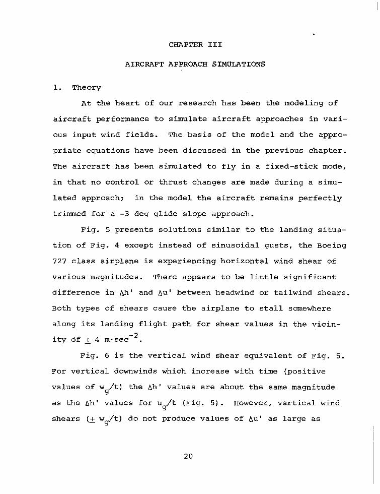
1. Theory

At the heart of our research has been the modeling of

aircraft performance to simulate aircraft approaches in vari-

ous input wind fields. The basis of the model and the appro-

priate equations have been discussed in the previous chapter.

The aircraft has been simulated to fly in a fixed-stick mode,

in that no control or thrust changes are made during a simu-

lated approach: in the model the aircraft remains perfectly

trimmed for a -3 deg glide slope approach.

Fig. 5 presents solutions similar to the landing situa-

tion of Fig. 4 except instead of sinusoidal gusts, the Boeing

727 class airplane is experiencing horizontal wind shear of

various magnitudes. There appears to be little significant

difference in Ah' and Au' between headwind or tailwind shears.

Both types of shears cause the airplane to stall somewhere

along its landing flight path for shear values in the vicin- -2 itydf+4m=sec . -

Fig. 6 is the vertical wind shear equivalent of Fig. 5.

For vertical downwinds which increase with time (positive

values of w,/t) the Ah' values are about the same magnitude

as the Ah' values for u d

t (Fig. 5). However, vertical wind

shears (+ w,/t) do not produce values of Au' as large as

20

E

f

Ah’ _F 200

a 1 \ Li

\ \

\ 100 - \

n- 1 I I I I I

-4 -2 0 2 4 HEADWIND TAILWIND

ug/t m -see-*

0

Fig. 5. RMS altitude and velocity deviations of a Boeing 727 class airplane to horizontal wind shears during a land- ing from 500 m altitude to the ground.

21

E F a

200 ,Au’

-

\- / \ / A ..I

100 -

0 -4 -2 0 2 4 6

UPWIND DOWNWIND

w,/t m - set-*

Fig. 6. R&IS altitude and velocity deviations of a Boeing 727 class airplane to vertical wind shears during a landing from 500 m altitude to the ground.

22

I -- ‘- --.

4 133 seconds (the normal landing time for descent from 500 m

those produced by + u d

t longitudinal wind shears. The large

values of Ah' produced by upwind shears are due to the fact

that after a certain amount of time has passed, the vertical

upwind is larger than the sink rate of the aircraft and the

airplane never lands, but continues to climb. The Ah' values

for upwind shears have been computed for a time interval of

with no wind). All other Au' and Ah' values shown in Figs. 4,

5 and 6 have been computed by the following formulae: t

L 1 Au' = [-

I u2dt]

s t (13)

Lo

% (h -hn)2dt] . (14)

2. Aircraft Simulations Using Real Data

The aircraft approach simulation model discussed in

part III (1) has been used with actual measured winds. The

two main sources for these winds have been 1) winds measured

by research aircraft during flight, and 2) winds measured

from a 444 meter-tall television tower.

(a) NCAR Aircraft Data

A prime source of data for winds near thunderstorms has

been the National Center for Atmospheric Research (NCAR)

Queen Air research aircraft. Such measurements were made,

principally in the lowest 1 km of the atmosphere, on several

days during the spring seasons of 1975 and 1977. These

23

aircraft are ideally suited for obtaining such data since

they cruise at a speed close to that of the approach speed of

a Boeing 727. The primary instrumentation system aboard the

research aircraft is a gust probe wind.measuring system cou-

pled to an inertial navigation platform, providing 1.0 Hz

sampling of the three-dimensional winds. Only the longitu-

dinal and vertical wind components are used in this study.

As mentioned, the data are 1.0 Hz samples of longitu-

dinal and vertical winds. The conventions of positive values

for tailwind and downwind have been used. Data from two days

have been used in the simulations. These days are 13 June

1975 (a day with tornadoes in Oklahoma) and 19 May 1977 (when

the aircraft flew in the vicinity of a squall line and through

the associated gust front). About two hours of data are avail-

able from each of the two flights. By initiating aircraft

approach simulations at 15 set steps into the data, a total

of 480 simulations per flight have been produced.

Figs. 7 and 8 give details of two sample simulations

from the 13 June 1975 data. Similar simulations have been

produced for other times that day and for 19 May 1977. The

heavy straight lines show the -3 deg glide slope centerline

and the so-called "missed approach" of -3 deg f: 0.7 deg.

The sequence of numbers "1" gives the actual aircraft posi-

tion for each 2 set from the initial time shown. The data

panels give 1.0 Hz values of u 9' w9' true airspeed (TAS),

24

140230 CST

20.0 -“““““~

FIXED - STICK SIMULATION USING

1~0230 -1o .. 13 JUNE 75 NCAR AIRCRAFT DATA _

-20.0 -

WG 140230

TAS 1110230

THE 1110230

5.0

0.0

-5.0

-10.0 w

180.0-

160.0 -

1110-o

120.0 -

lOO.O- 15.0 10.0 5.0 E

z! ” .30

I=

ii? .25 >

.20

.15

.lO

.OS

0.0 1 0.0 --

.I. .~ . I .-_ - L .---L- I I I

HORIZONTAL%STANCE [KM]

Fig. 7. Fixed-stick model simulation using NCAR aircraft data for 13 June 1975 at 140230 CST. Data panels show u and TAS and 0 output, with time increasing to the r ght, wrth 9' wg input each division 10 sec. Larger panel shows aircraft position with respect to -3 deg + 0.7 deg glide slope to nominal touch- down at lower right. Case demonstrates that seemingly turbu- lent input results in relatively good approach.

25

---

.75

.70

.65 20.0 m

10.0

UG 0.0 1~815 -1o.o

-20.0 i/‘i

.60

.55 J

10.0 5.0 - To

WG 0.0 .‘15

142815 -5.0 k--i : cl -Lfo

-10.0 w 180.0

160.0

TAS 140.0 1vx3*5 120 -0

100.0 15.0 10.0

THE ::i 192815 -5.0

-10.0 -15.0

-10

.OS

142815 CST

FIXED - STICK SIMULATION USING

13 JUNE 75 NCAR AIRCRAFT DhTA

0.0 0.0

HORIZONTAL ‘I%TANCE [KM]

Fig. 8. Same as Fig. 7, for starting time of 142815 CST. Demonstrates non-turbulent but high shear input results in poor approach.

26

and pitch angle (6). The first case is interesting in that

the approach is "quite good" since departures from nominal

[TAS = 72.1 mesec-' (140 kt) and "on the beam"] are small,

even though the input winds appear to be turbulent. The

second case (Fig. 8) demonstrates a situation where the de-

parture from the glide slope is extreme, while turbulent

velocity deviations are relatively minor.

To better quantify these "departures", variables Au'

and Ah', as defined by Eqs. (13) and (14), were calculated

for the 480 simulations for each day. Each quantity Au' and

Ah’, can be considered as Approach Deterioration Parameter

(ADP) under the assumption that significant velocity devia-

tions from the nominal true airspeed and height deviations

from the glide path represent deterioration of the approach.

Table 2 gives the appropriate values for the example cases.

Table 2. Approach Deterioration Parameters and shear values for the two examples given in Figs.2 and 8, 13 June 1975.

-.. --- - Au' Ah' (Ugml Gp30 (q7q (Wg/t)30

Time m-set -IL m m=sec -2 -2 m=sec -2 -2 m-set m-set 140230 1.6 14.8 1.06 0.078 0.63 0.040

142815 2.5 193.7 0.26 0.176 0.09 0.017 -___-.-

An attempt has been made to correlate shear values for

ug and w

g' to the values. of ADP. Table 3 gives the least-

squares linear regression correlation coefficients for four

shear values. The subscripts indicate the number of seconds

27

for which the mean shear is calculated. Clearly for the Au'

parameter, reasonably high correlations occur, while for Ah'

no significant relationship appears, especially for the 13

June 1975 data. The fact that Au' is highly correlated and

Ah' is less highly correlated can be understood by examining

the relationship between Au', Ah' and the shears as seen in

Figs. 5 and 6. Au' is seen to plot as very nearly straight

lines in Figs. 5 and 6 while Ah' does not, and is, in fact,

a rather complex non-linear function.

Table 3. Least-squares linear correlation coefficients be- tween indicated shears (independent variable) and two Approach Deterioration Parameters for 480 simulations (13 June 1975 data). Values for 19 May 1977 data are shown in parentheses.

Shear Values Au'

-1 (m-set ) Ah'

(m)

(0.63)

0.68

(0.50)

(u,7t),O 0.35

(0.47)

0.69

(0.46)

0.70

(0.47)

0.09

(0.62)

0.30

(0.37)

0.10

(0.43)

0.01

Variance spectra, as described in part II (3) have been

found for each of the first 470 input data sets for the two

28

research days (13 June 1975 and 19 May 1977). Each spectrum

is calculated at 251 frequencies from 0.0 to 0.5 Hz. For

frequencies at regular intervals, a least-squares fit is made

correlating 470 pairs: the energy density at a given fre-

quency and the value of Au' for that simulation. A first ,

order correlation coefficient is calculated for each fre-

quency. Fig. 9 contains plots of the square of the correla-

tion coefficient (positive correlation) against frequency for

the two days. Two curves are shown in each plot, one for u g

and one for w g-

Correlations have been run for the special

case of w ph (.026 Hz) and are shown with the small x's.

These results support the ideas presented in Fig. 4.

That is, Au' is greater when a large amount of energy is pre-

sent in the u g field centered about the phugoid frequency.

In other words, there is a strong linear relationship between

Au' and high energy density at w ph'

a relationship which

breaks down at frequencies significantly different from u) ph'

However, a similar correlation peak is not seen in the w g

field at wph, nor, from Fig. 4, would it be particularly im-

portant for aircraft approach quality were it present. Clear-

ly then, we can conclude that longitudinal wind gusts provid-

ing energy at the phugoid frequency may result in airspeed

oscillations of a nature that would be difficult to control,

and in fact may lead to stall, and otherwise disastrous re-

suits.

29

1.0

0.8

Ns 0.6 0 -

0.2

0.0 0.01 .026 0.1 0.5 I- _I

I I I I IIIII

- ug SPECTRA 13 JUNE 75 - wg SPECTRA (a)

1.0

0.8

Ns 0.6 0

2

=

E

0.4

E

0.2

0-C

FREQUENCY [Hz]

I I I I I I I I ~-7-I

- ug SPECTRA 19 MAY 77 - wg SPECTRA lb)

0.01 ,026 FREQUENCY $1

Fig. 9. The square of the least-squares correlation co- efficient (variance explained) plotted against frequency for (a) 13 June 1975 and (b) 19 May 1977. See text for explanation.

30

The Au' values are plotted as functions of the peak value of

the ARWS [discussed in part II (3)] in Fig. 10. Again both

days are shown. The ARWS appears to be a better predictor

for estimating approach quality. Close inspection of Fig. 10

shows.that ambiguities remain, since a precise Au' cannot be

predicted from a given ARWS. Instead, only a critical thres-

hold can be seen, beyond which large values of Au' might occur.

An unanswered question is what value of ARWS is critical?

This question will be addressed in part III (3).

(b) KTVY Tower Data

Another source of data has been space-time adjusted

fields of winds from the 444 meter instrumented KTVY-TV tower

located in northern Oklahoma City, Oklahoma. Twenty thunder-

storm influenced cases have been used to produce input winds

for the simulation model. Approach wind conditions are ob-

tained along approach paths in each direction through the two

dimensional data fields. Also turbulence has been added by a

numerical model of turbulence to create a second set of 40

input winds for simulations. Thus a total of 80 approach

wind inputs are available for use in the Boeing 727 simula-

tion model. Tower data were processed by use of a computer

program developed by Frost et al. (1978). --

Samples of these simulations are shown in Figs. 11 and

12. These show extreme cases of aircraft performance. Fig.

11 shows input winds with small scale turbulence but no large

31

I I I I, I, 1 , I,, I,,

13 JUNE 75 -

. **-.. . *: - . * ..j * .* . *.. ‘. .

-- -2 :. . . . ‘f. . .*. . 1.

----- ------___- ‘z. -. ‘. - I .-.-m.’ .L ;* -

hmJ ;y-“y-?. 1 -* . :- J :* ‘-‘. . .

. . 2:‘I . ...-‘+. : ’

. :. . . ,..L’ - C...‘-‘-‘:.f..‘. , L .--.:- I e-s:.. * .I.’ - .:.“-..-: -7, : .: .- * :-‘*’ . ” .* .; . .“W A r - -

. ..1..* t&-L-.-’ - .I . . .* - ‘*k~-&- * - w = r.““’

0.0 1

: . * 1

I I I I I I I 0.0 10.0 20.0 30.0 40.0 50.0 60.0 70.0 60.0 90.0

ARWS FUNCTION m25ecz i 1 ~z (dB)

Fig. 10. SCattergramS relating AU’ t0 ARWS function, expressed in dB, for (a) 13 June 1975 and (b) 19 May 1977. JFK accident ex- amp_ls shows a computed ARWS value of 65 m2. set -HZ-~ predicts a Au' RMS velocity de- parture of 3.5 mmsec-1.

32

.65

.;::: R .60

UG 0-o ~00011 -1l-J.o

WG 00001

TFlS 0000 1

-2o.oL 10.0

5.0

0.0

1 -5.0

-10.0 1

160.0

160.0

140.0

l 120.0

100.0 :

-;s.o- .lO

.05

0.0 0.0

HORIZONTAL D?TANCE [KM]

Fig. 11. Same as Fig. 7, for a sample simulation using tower data. Demonstrates small amplitude turbulence with a good approach.

33

LIG

WG 000020

TflS 000020

20.0 10.0

0.0

,lO.O

-20.0

Y-l -

10.0

5.0

0.0

-5.0

-10.0 I---1

180.0

160.0

1110.0

120.0

100.0 l--+4

.20

THE 000020

Fig. 12. Same as Fig. 7, for a sample simulation using tower data. Demonstrates wave-like input which results in a poor approach.

.70

.65

.60

34

fluctuations over sustained time periods. The aircraft per-

formance is good with only slight airspeed changes. The air-

craft does drift somewhat below the glide slope due to the

downdraft (positive wg). In Fig. 12, a large change in u g

over a number of seconds produces rather large fluctuations

in airspeed and aircraft height.

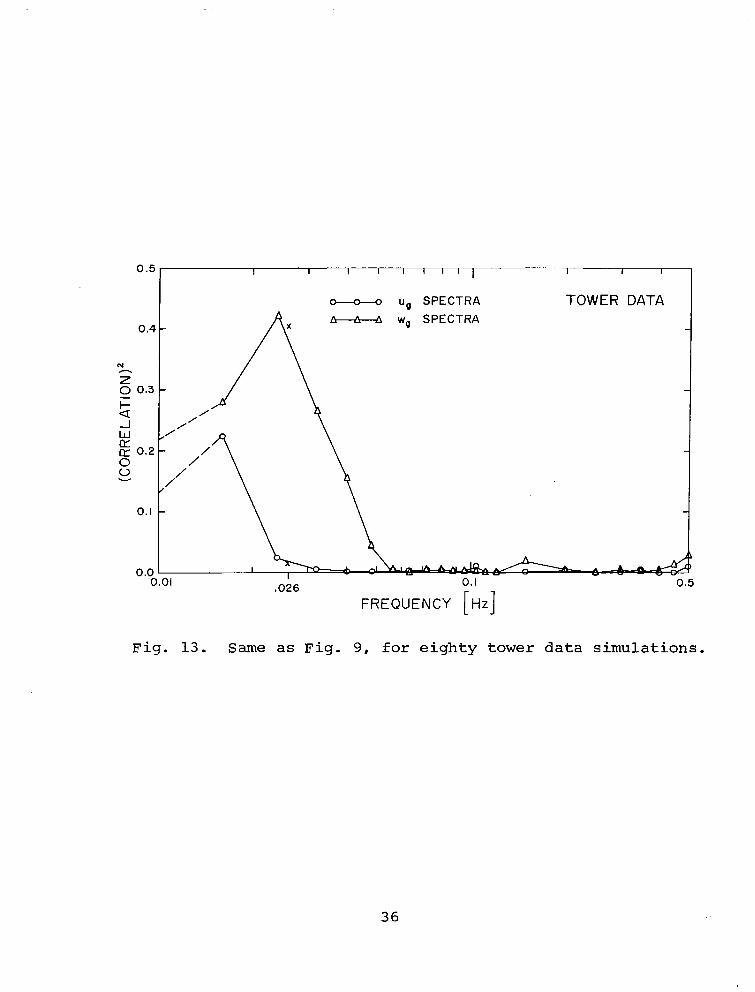
Fig. 13 is comparable to Fig. 9 except it is for the 80

tower wind cases. Notice that the results are different.

The correlations are smaller and the peak for the u cl

spectra,

near the phugoid frequency, is not seen. The smaller sample

size (80 vs. 470) may be a factor in these differences.

Fig. 14 includes scattergrams for Au' as a function of

the peak value of ARWS. Three sets are included: 1) 40 cases

of data with no turbulence added, 2) 40 cases with turbulence

added, and 3) 80 cases consisting of the combination of both.

The patterns are rather similar in each plot and agree with

the larger sample shown in Fig. 10, and the conclusions reach-

ed in the discussion of Fig. 10 apply here as well.

3. An Example: JFK Crash, 1975

The tragic crash of Eastern Airlines Flight 66 at JohnF.

Kennedy Airport on 24 June 1975 has focused the attention of

aeronautical engineers and meteorologists on the problem of

landing aircraft in thunderstorm related environments. The

National Transportation Safety Board in NTSB (1976a) has

stated that the probable cause of Eastern Airlines' Flight 66

35

0.5

0.4

N

s 0 0.3 i= a

I I I I I IllI

- ug SPECTRA

X

I A

- wp SPECTRA

0.0 a 0.01 ,026

0.5

Fig. 13. Same as Fig. 9, for eighty tower data simulations.

36

.- -

5.0

4.0

1.0

0.0 (

4.0

c-- 1 g 3.0

fn

L 2 2.0

1.0

Lo, I I I I I I I I I I I I I , , ,

.

. . .

.

. . . . . .

. . . .

. . . . .

m . . .

. . I I I I I I I I.1 I l I, l , , ,

10.0 20.0 30.0 40.0 50.0 60.0 70.0 at.0 90.0

ARWS FUNCTION

. . . . .

.

. .

. . . . . .

. .

. . .

. .

. . . .

. . m . . . . .

. .

. . . .

. .

.

0.0 I-- 0.0 IO.0 20.0 30.0 40.0 50.0 60.0 70.0 60.0 90.0

ARWS FUNCTION m2sec-2 [ 1 - (dB) HZ

Fig. 14. Plots same as Fig. 10, for (a) tower data cases, (b) tower data cases with turbulence added and (c) both (continued on next page).

37

5.0

4.0

7 ‘0 3.0

2

L

2 2.0

I .o

, I I I I I I I I I I I I I I I I

(c)

. . . .

. . . . . .

I .

.

. . . . . . . . . . . . . .

. . . .

.m. :=. . ..m. . . I

: .” . .

“._I . .

. . . . . . III I, I I I I I I I I I I I I 0,o L

0.0 10.0 20.0 30.0 40.0 50.0 60.0 70.0 80.0 90.0

ARWS FUNCTION

[ m2sec2 - Hz 1 MB)

Fig. 14. continued.

38

accident was 'I . ..an encounter with adverse winds associated

with a very strong thunderstorm located astride the ILS local-

izer course which resulted in a high descent rate into non-

frangible approach light towers."

We have examined the Eastern 66 crash using the Boeing

727 simulation model. Although data are sparse for the winds

encountered by the aircraft, the relatively simple descrip-

tion of the winds found in NTSB (1976a) is used here. Fig. 15

gives the u and w g (3

wind components taken directly from the

NTSB report (page 17), and placed on a simulated -3 deg glide

slope approach. Fig. 16(a) gives the simulated position of

the aircraft relative to the ILS corridor, while 16(b) gives

the simulated true airspeed. Three cases have been run:

% with w

4 = 0, wg with u = 0, and u w ,

g 9-g all using the fixed-

stick mode.

Several interesting observations can be made, related

in particular to Fig. 4. When u g

is taken alone, input is

an apparent one-half wave of period of approximately 19 set,

or a full wave of 38 set; for such a wave the energy is con-

centrated at 0.026 Hz, precisely the phugoid frequency! We

give computed values of ADP as a function of frequency, so

comparisons to Fig. 4 might be made; such a comparison for

the u g

case is quite good. The case of the w g

fluctuation

must be considered in a little more detail. In Fig. 15, we

see more of a pure shear of -10.8 mesec -1 over about 12 set,

39

HEIGHT ABOVE RUNWAY [M] 500 400 300 200 100 0

I I I I

14 t I

3-S - \

\

\

-8 - \

\

-10 -

\

\ .--------m-s-

-12 -

I I I I I I I I I I I ,-..I

0 IO 20 30 40 50 60 70 80 90 100 110 120 130

TIME [set]

-14 -

Fig. 15. Longitudinal and vertical environment winds encountered by Eastern Flight 66, as derived from NTSB (1976a). Subjective smoothing was applied to the data: no turbulence fluctuations were added. A ug headwind and a wg updraft are positive.

40

a I "aWa< X\-"Gi

W I Y

82.4 (160)

52

5 77.2 (150)

'0 $72,1 (140)

D 66.9 (130) W W CL

$ 61,8(120)

56,6(llO) “gWg

I I I I I , I I

0 I 2 3 D;STANC: [KM61

7 8

(b)

I

9 IO

Fig. 16. (a) Model output showing airplane position relative to glide path. Curves are shown for three input environmental winds: longitudinal ug, vertical wg, and both ug and w . (b) Model out- put showing airplane airspeed for three cases 1 airspeed is 72.1 masec-1 (140 kt).

'sf (a). Nominal

41

rather than a wave feature. To relate shear to harmonic fea-

tures, a Fourier analysis of simple shear is performed, sug-

gesting most of the energy density is represented in a sine

wave with a 12 set period. Consequently we can consider the

a.ppropriate frequency to be .083 Hz or UJ/W Ph

= 3.21, as seen

in Table 4. From Fig. 4, this frequency clearly represents a

small deterioration of approach quality, as seen in the esti-

mated Au' and Ah'. Notice that the ADP's for W/W Ph

= 3.21 in

Fig. 4 are far below those calculated and given in Table 4.

This difference may be due to the fact that we are comparing

ADP estimates of two highly simplified models: however, the

example serves to illustrate the point that the aircraft re-

sponse to w g

is considerably less than its response to u 4.

Table 4. Approach Deterioration Parameters for JFK simula- tion (refer to Figs. 15 and 16 for profiles).

Case Au'

-1 m*sec Ah’ w w/w Ph 0-d (Hz)

ug only 3.5 23.7 .026 1.00

wg only 0.9 20.4 -083 3.21

%’ wg 3.8 22.6

Returning to the full simulation, note that fluctuations

in velocity from 72.1 m=sec -' (140 kt) are large indeed, re-

sulting in a wave-like departure from the nominal value. In

terms of the hu' ADP, most of the deterioration occurs because

42

of the u factor. 4

In fact, the calculated values of Au' and

4h' agree quite well with the predicted values given in Fig. 4,

for the appropriate value of U/W ph'

We see that the largest

values of ADP should be associated with u g'

and the most sen-

sitive indicator is the Au' ADP. Referring again to Fig. 16,

we see that the extreme airspeed oscillation associated with

% bears this out.

The deleterious effect of w CJ

is present, as seen in the

glide slope position plot: however, we contend that the most

critical feature is the extreme oscillation in airspeed, due

to the aircraft's encounter with high energy at the phugoid

frequency.

Inspection of Fig. 4 indicates a large peak in the rela-

tionship between w and Ah', -3 g

near w = 4.7 x 10 Hz represent-

ing a wave period of 214 sec. We assume that a real pilot

easily would be able to overcome such an effect by elevator

and thrust corrections, since the time-space scale length is

61% longer than the 133 set nominal approach period. Use of

the fixed-stick mode precluded such a correction here.

The utility of the ARWS function can be seen in the JFK

simulation. For example, a Au' of 3.5 m=sec -1 requires the

product of u 53

energy density and transfer function be at

least 65 m20sec-2-Hz -1 expressed in dB; as shown in Fig. 10.

For the Eastern 66 simulation, this value of ARWS presumably

represents a critical threshold.

43

L

To obtain an estimate of the frequency of occurrence of

conditions comparable to those experienced by Eastern 66, the

% energy density at the phugoid frequency for the 940 near-

thunderstorm wind profiles was examined. The cumulative fre-

quency for multiples of the energy density obtained from the

wind profile used in the Eastern 66 simulation is shown in

Table 5. It can be seen that for these near-thunderstorm

conditions, the energy density at the phugoid frequency ex-

ceeds the Eastern 66 value for about 8% of the cases and is

more than double that value for almost 2% of the cases. This

demonstrates that flying conditions as bad as those experi-

enced by Eastern 66 are not extremely rare.

Table 5. Cumulative frequency distribution of energy density at phugoid frequency, as a function of multiples of Eastern66 computed energy density for ug at fJ.Iph. Tower data values are in parentheses.

Multiples of Eastern 66 Energy Cumulative Density of 95.24 m2-set -2 -Hz-l Frequency

0.25 0,373 (0.700)

0.50 0.203 (0.363)

0.75 0.114 (0.225)

1.00 0.078 (0.200)

1.25 0.051 (0.138)

1.50 0.029 (0.125)

1.75 0.022 (0.088)

2.00 0.017 (0.050)

44

Included in Table 5 are the cumulative frequencies for

the 80 tower data cases. It can be seen that 20% of these

cases exceed the value of Eastern 66. The results are com-

parable to the 940 aircraft cases but frequencies are some-

what higher.

In conclusion, we believe that the JFK accident is as-

sociated with the airplane's encounter with a horizontal wind

containing high energy at the airplane's critical phugoid fre-

quency, which caused a sudden extreme variation in the air-

speed. Matters were made worse by the downdraft, but the air-

plane's response was most seriously affected by u variations. 53

We see this explanation as a subtle but important variation

from the conclusion of Fujita and Caracena (1977) that a sud-

den "downburst" drove Eastern 66 into the ground. Their ex-

planation does not consider aircraft response stability as a

vital parameter, and leaves the impression that the accident

was caused entirely by meteorological events. Our explana-

tion certainly includes meteorological events, including a

possible downdraft as an initiating factor, but extends the

concept to couple aircraft response factors to the weather.

The horizontal wind ug, perhaps caused by thunderstorm out-

flow, provides energy at the phugoid frequency, excites a

severe horizontal velocity oscillation, leading to loss of

control and a possible stall. Furthermore, we must not over-

look the reality that an aircraft is likely to encounter

45

horizontal gustiness more frequently than vertical "downbursts".

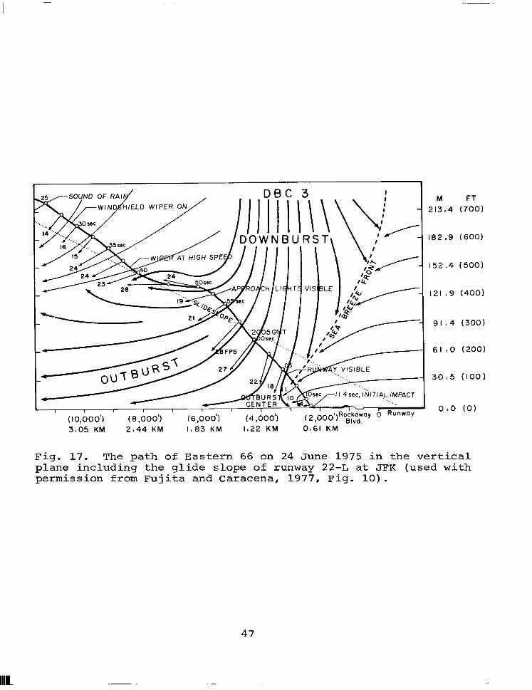
At this point it is very interesting to compare Fujita's

(1977) analysis of Eastern 66 to our model results seen in

Fig. 16. .Fig. 17 (from Fujita and Caracena, 1977) shows the

flight track of Eastern 66, in a view similar to Fig. 16(a).

There is a remarkable similarity between his analysis which

requires the downburst explanation, and our u curve which (3

includes no w 4

component. True, then w g

is added, matters

are made slightly worse, but the basis of our alternative

explanation is made clear. We must conclude that a consid-

eration of aircraft response theory, as well as environment

wind energy, is necessary to fully appreciate the approach

hazard.

46

-- -

i\\\ i

(lO,bOO’, (8,000’) (6,000’) (4,000’) ( 2 ,ooo’PO,~g,WC

3a05 KM 2844 KM In83 KM I*22 KM Oa6i KM

M 21304

182.9

152.4

91,4

61 10

3085

ouo

FT

(700)

(600)

(500)

(400)

(300)

(200)

(100)

(0)

Fig. 17. The path of Eastern 66 on 24 June 1975 in the vertical plane including the glide slope of runway 22-L at JFK (used with permission from Fujita and Caracena, 1977, Fig. 10).

47

CHAPTER IV

CONCLUSIONS

The work reported herein represents an attempt to com-

bine fundamental aircraft response to the thunderstorm envir-

onment wind shear, during an approach-to-landing. Not only

have we developed several means of examining the nature of

the wind shear, but we have mated it to the basic response

characteristics of aircraft. This has resulted in a means

to predict the possible deterioration of the approach, for

given wind conditions and for a specific aircraft type. We

have chosen only one aircraft type for our study, a medium-

sized jet transport (Boeing 727 class) as a convenience, and

not in any way to single out this airplane, but to represent

a typical airliner.

Our examination indicates the presence of wind shear

containing energy at our aircraft's resonant or phugoid fre-

quency sufficient to suggest serious deterioration of the

approach on about 20% of approximately 1000 cases examined.

This deterioration is observed as sudden oscillation in air-

plane airspeed that can bring the aircraft near stall, or in

height oscillations from the glide slope, possibly bringing

about a premature impact with the ground short of the runway.

For our aircraft of study, the phugoid frequency is

0.026 Hz, or for an approach speed of 72.1 m-set -' (140 kt)

48

a phugoid wavelength of 2.8 km. We are not surprised by our

finding that approximately 20% of our cases had phugoid energy

sufficient to suggest approach deterioration equal or worse

than that encountered .by Eastern--Flight' 66. Such a scale

length (near 3 km) would be a typical one in a thunderstorm,

for vertical columns (updrafts and downdrafts) occur on such

a horizontal length scale. Our study suggests that horizon-

tal variations of the environmental wind along the aircraft's

longitudinal axis of motion, are more critical than vertical

variations of wind. While these vertical components can de-

teriorate the approach, it appears that a firm handle on the

horizontal component is most important.

Consequently,~ we b-elieve critical energy at the phugoid

frsquency- -i-sat least not rare in the thunderstorm landing --

environment, and therefore the national airspace system should

take steps to detect and warn approaching aircraft of such

problems. It is important to realize that this conclusion

about the nature of wind shear is fundamentally a time depen-

dent problem. The existence of atmospheric waves, whose ef-

fect on aircraft depends on approach speed as well, requires

time variation considerations. Previous wind shear studies

have not denied this important point, but have failed to

recognize it as critical.

Our work has limitations, to be sure. First of all, it

is theoretical in that we simulate flight, rather than consider

49

a real aircraft. Furthermore, no pilot is considered. Some

will suggest that our conclusions are severely limited by this

exclusion. We cite our sensitivity studies of elevator input

in Chapter II and our Eastern 66 simulation in Chapter III as

indicating that phugoidal response problems are still serious

when pilot input is included. Finally, we have examined only

one type of aircraft. While this of course limits the scope,

our objective is not to identify positively whether a speci-

fic airplane will in fact crash, but rather to indicate the

fundamental nature of the wind shear - aircraft interaction.

This interaction exists for all aircraft, but a given wind

field may have less serious consequences for some aircraft

(our Beech Baron at JYFK, for example).

Where do we go from here? We believe a real-time ap-

proach deterioration parameter detection system may be fea-

sible. The system would work as follows:

1. A single pulsed Doppler radar would collect radial

velocities (from the ground) along intended ILS

glide paths to airport runways. These radial com-

ponents would be essentially identical to u com- g

ponents discussed in this work, after making a

frozen turbulence hypothesis. Remember, our work

has indicated the u 9-

component should be a good

"trouble" predictor.

2. The u data would be collected at discrete distances g

50

I

along the glide path, then converted to the time

series input form by knowing the aircraft approach

speed. This u g

as a function of time would be fed

into the simulation model, which would be adjusted

for a type of aircraft.

3. The model output would predict an ARWS parameter

which could be used by the ATC controller and/or

pilot to decide whether severe conditions exist

along the intended approach.

The advantages of this system could be many. It would not

require an actual and possible dangerous approach to be util-

ized. A quantitative estimate of ADP would be available at

all times. The ADP would be mated to aircraft type (although

we do not expect the system to be used to let some aircraft

to land, while forcing others to go around).

The authors are in the process of testing the feasi-

bility of such a system, with the hopes that an operational

system could be implemented in the early 1980's.

51

REFERENCES

Frost, W., and B. Crosby, 1978: Investigations of simulated aircraft flight through thunderstorm outflows. NASA Contractor Report 3052, 110 pp.

and K. R. Reddy, 1978: Investigation of aircraft ianding in variable wind fields. NASA Contractor Report 3073, 84 pp.

D. W. Camp, and S. T. Wang, 1978: ;or aircraft hazard definition.

Wind shear modeling FAA Report NO. FFA-RD-

78-3, 240 pp.

Fujita, T. T., and H. R. Byers, 1977: Spearhead echo and down- burst in the crash of an airliner. Mon. Wea. Rev., 102, 129-146.

and F. Caracena, 1977: An analysis of three weather- belated aircraft accidents. Bull. Amer. Meteor. Sot., 11, 1164-1181.

Goerss, J. S., and A. J. Koscielny, 1977: Monte Carlo estima- tion of confidence limits for maximum entropy spectra. Preprints 5th Conf. Prob. and Stat. in the A.tmqs.. ~ci., La.5 Vegas, Amer. Meteor. Sot., 297-302.

McCarthy, J., and E. F. Blick, 1976: Aircraft response to boundary layer turbulence and wind shear associated with cold-air-outflow from a severe thunderstorm. Pre- prints 7th Conf. Aerospace a

Melbourne, S ymposium on Remote Sensing from Satellites, Fl., Amer. Meteor. Sot., 62-69.

and R. R. Bensch, 197873: A spectral analysis Lf thund&storm turbulence and jet transport landing performance. COnf. Atmos. Environment of Aerospace Systems and Applied Meteor., New York, Amer. Meteor. sot.

Af wind iurbulenhe and N. R. Sarabudla, 1978a: Effect

and shear on landing performance of jet transports. Preprints 16th AIAA Aerospace Sciences Meeting, Huntsville, Al., Amer. Institute of Aeronautics and Astronautics.

McRuer, D., I. Ashkenas, and D. Graham, 1973: Aircraft Dyna- mics and Automatic Control. Princeton Univ. Press, 313~~.

52

National Transportation Safety Board, 1974: Accident Report - Delta Airlines, Inc. Douglas DC-9-32, Chattanooga Mu- nicipal Airport, Chattanooga, Tennessee, November 27, 1973; NTSB-AAR-74-13, Washington, D.C.

, 1976a: Accident Report - Eastern Airlines, Inc. BOe- ing 727-225, John F. Kennedy Airport,-Jamaica, New York, June 24, 1975, NTSB-AAR-76-8 Washington, D.C., 47 pp.

, 1976b: Accident Report - Continental Airlines, Inc. Boeing 727-224, StapeltOn InternatiOnal Airport, Denver, Colorado, August 7, 1975; NTSB-AAR-76-14, Washington, D.C.

Roskam, J., 1972: Flight Dynamics of Rigid and Elastic Air- planes, Part 1. Pub. by author, 519 Boulder, Lawrence, KS., 619 pp.

Ulrych, T. J.,and T. N. Bishop, 1975: Maximum entropy spec- tral analysis and autoregressive decomposi.tion. Rev. Geophysics and Space Physics, 13, 183-200. -

53

RECIPIENT’S CATALOG NO.

NASA CR-3207 4. TITLE AND SUBTITLE 6. REPORT DATE

December 1979 Jet Transport Performance in Thunderstorm Wind Shear 6. PERFORMING ORGANIZATION CODE

Conditions 7. AUTHOR(S) 6. PERFORMING ORGANIZATION REPI3R.r #

John McCarthy, E 9. PERFORMING ORGANIZATION NAME AND ADDRESS 10. WORK UNIT, NO.

M-290

D

The University of Oklahoma Norman, Oklahoma

11. CONTRACT OR GRANT NO.

NAS8-31377 ,S. TYPE OF REPOR-; & PERIOD COVERE

12. SPONSORING AGENCY NAME AND ADDRESS

National Aeronautics and Space Administration Washington, D. C. 20546

15. SUPPLEMENTARY NOTES

Contractor

14. SPONSORING AGENCY CODE

Prepared under the technical monitorship of the Atmospheric Sciences Division, Space Sciences Laboratory, NASA Marshall Space Flight Center

16. ABSTRACT

Several hours of three-dimensional wind data were collected in the thunderstorm approach-to-landing environment, using an instrumented NCAR Queen Air airplane. These data were used as input to a numerical simulation of aircraft response, concentrating on fixed-stick assumptions, while the aircraft simulated an ILS approach. Output included airspeed, vertical displacement, pitch angle, and a special approach deterioration parameter. Theory and the results of approximately 1000 simulations indicated that about 20 percent of the cases contained serious wind shear conditions capable of causing a critical deterioration of the approach. In particular, the presence of high energy at the airplane’s phugoid frequency was found to have a deleterious effect on approach quality. Oscillations of the horizontal wind at the phugoid frequency were found to have a more serious effect than vertical wind. A simulation of Eastern Flight 66, which crashed at JFK in 1975, served to illustrate the points of the research. A concept of a real-time wind shear detector was outlined, utilizing these results.

7: KEY WORDS

Thunderstorm Wind shear Phugoid frequency Aviation safety Wind spectra Flight simulation

9. SECURITY CLASSIF. (of thlm rap&t) 20. SECURITY CLA!

16. DISTRIBUTION STATEMENT

Category 47

IF. (of thi* P=o*) 21. NO, OF PAGES 22. PRICE

Unclassified Unclassified I 61 SFC-Form3292 (Rev.DecemberlS72) For aale by Nationd Technical Informdion Scrvke. Srwidield. vti- 2 2 13 1

NASA-Langley, 1979