Effective Storm-Relative Helicity and Bulk Shear in ... · Effective Storm-Relative Helicity and Bulk Shear in Supercell Thunderstorm Environments RICHARD L. THOMPSON,COREY M. MEAD,

Effective Storm-Relative Helicity and Bulk Shear in SupercellThunderstorm Environments

RICHARD L. THOMPSON, COREY M. MEAD, AND ROGER EDWARDS

Storm Prediction Center, Norman, Oklahoma

(Manuscript received 22 August 2005, in final form 1 June 2006)

ABSTRACT

A sample of 1185 Rapid Update Cycle (RUC) model analysis (0 h) proximity soundings, within 40 km and30 min of radar-identified discrete storms, was categorized by several storm types: significantly tornadicsupercells (F2 or greater damage), weakly tornadic supercells (F0–F1 damage), nontornadic supercells,elevated right-moving supercells, storms with marginal supercell characteristics, and nonsupercells. Theseproximity soundings served as the basis for calculations of storm-relative helicity and bulk shear intendedto apply across a broad spectrum of thunderstorm types. An effective storm inflow layer was defined interms of minimum constraints on lifted parcel CAPE and convective inhibition (CIN). Sixteen CAPE andCIN constraint combinations were examined, and the smallest CAPE (25 and 100 J kg�1) and largest CIN(�250 J kg�1) constraints provided the greatest probability of detecting an effective inflow layer within an835-supercell subset of the proximity soundings. Effective storm-relative helicity (ESRH) calculations werebased on the upper and lower bounds of the effective inflow layer. By confining the SRH calculation to theeffective inflow layer, ESRH values can be compared consistently across a wide range of storm environ-ments, including storms rooted above the ground. Similarly, the effective bulk shear (EBS) was defined interms of the vertical shear through a percentage of the “storm depth,” as defined by the vertical distancefrom the effective inflow base to the equilibrium level associated with the most unstable parcel (maximum�e value) in the lowest 300 hPa. ESRH and EBS discriminate strongly between various storm types, andbetween supercells and nonsupercells, respectively.

1. Introduction

Supercell thunderstorm environments, from both ob-servations and numerical simulations, typically consistof relatively large buoyancy and vertical shear througha substantial depth of the troposphere. Numerical simu-lations (e.g., Weisman and Klemp 1982, 1984, 1986;Weisman and Rotunno 2000) have established thatstrong vertical wind shear, generally greater than 20–25m s�1 wind variation over the lowest 4–6 km aboveground level (AGL), is necessary for the maintenanceof long-lived supercell structures. Sufficient verticalshear through this depth allows for the establishment ofthe characteristic mesocyclone structure in right-moving supercells, such that precipitation and associ-

ated evaporative cooling do not disrupt low-level storminflow (Weisman and Rotunno 2000; Rotunno andWeisman 2003). Though some disagreement exists re-garding the influence of low-level shear versus deep-layer vertical shear in supercell propagation [e.g., theDavies-Jones (2002) and Rotunno and Weisman (2003)exchange], it is generally accepted that the primarysource for midlevel rotation in supercell thunderstormsis the tilting and stretching of streamwise vorticity(Davies-Jones 1984). Davies-Jones et al. (1990) devel-oped storm-relative helicity (hereafter SRH) as ameans to quantify streamwise vorticity as a forecasttool for supercell and tornado environments.

A concern with the previous numerical simulations,and subsequent observational investigations, is thatSRH calculations have been tied to somewhat arbitrarylayers AGL. Predictive estimates of SRH have also re-lied on various storm motion algorithms (most recentlyBunkers et al. 2000) in combination with approxima-tions to the storm inflow layer (typically the lowest 1–3km AGL). In an attempt to refine the estimates of the

Corresponding author address: Richard L. Thompson, StormPrediction Center, 120 David L. Boren Blvd., Suite 2300, Norman,OK 73072.E-mail: [email protected]

102 W E A T H E R A N D F O R E C A S T I N G VOLUME 22

DOI: 10.1175/WAF969.1

WAF969

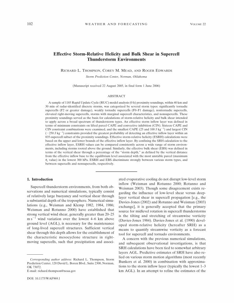
storm inflow layer, the depth of the inflow layer is con-strained by the vertical profiles of temperatures andmoisture. Specifically, it is assumed that only lifted par-cels associated with CAPE will sustain a deep thunder-storm updraft, whereas parcels associated with verylarge convective inhibition (CIN) will ultimately resultin storm demise.1 A sample of 1185 close proximitysoundings, derived from RUC model hourly analyses,served as the basis for our estimates of the storm inflowlayer.

In determining relevant bounds on a storm inflowlayer, the likelihood of detecting a storm inflow layerand the error characteristics of the RUC analysissoundings both are quite important. Thompson et al.(2003, hereafter T03) compared a sample of 150 RUCanalysis (0 h) and 1-h forecast soundings to observedsoundings within 3 h and 185 km of observed supercellsand found that the RUC soundings tended to be toocool and dry at the surface (Figs. 2a and 2b in T03).These cool and dry biases resulted in 100–250 J kg�1

underestimates of CAPE (after Doswell and Rasmus-sen 1994) in typical cases (Fig. 3 in T03), and CIN val-ues that were too negative (not shown). Assigning aCAPE threshold too large or an absolute CIN thresh-old too small lowers the probability of identifying astorm inflow layer within a proximity sounding, whichcompounds the aforementioned RUC sounding biases.Modification of the proximity soundings with nearbysurface observations counters the RUC analysis biasesat the ground.

Distributions of most unstable parcel (maximum �e

value in the lowest 300 hPa) CAPE and CIN from our1185 proximity soundings suggested the following po-tential inflow layer constraints: CAPE values of 25, 100,250, and 500 J kg�1, and CIN values of �50, �100,�150, and �250 J kg�1 (16 possible combinations).These tested thresholds of CAPE and CIN all fell wellwithin the lowest 10% of values for all 1185 proximitysoundings, and above the minimum values of the mostunstable parcel CAPE and CIN in our sample (4 and�381 J kg�1, respectively).

Beginning at the ground level in each sounding andsearching upward, lifted parcel CAPE and CIN valuesassociated with each level in the sounding were com-pared to each of the 16 possible constraint combina-tions. The first level that met both of the constraints

(i.e., CAPE � 100 J kg�1 and CIN � �250 J kg�1)became the “effective inflow base.” Continuing up-ward from the effective inflow base, the effective in-flow layer consisted of all contiguous parcels that metboth constraints, and the last parcel meeting the con-straints became the “effective inflow top.” The verti-cal distance between these two levels defined the effec-tive storm inflow layer, and established the verticalbounds on the calculation of effective SRH (hereafterESRH).

Observational studies of proximity soundings (e.g.,Rasmussen and Blanchard 1998; T03) have confirmedthat vertical wind shear over the lowest 6 km AGL2 isa strong discriminator between supercell and nonsuper-cell thunderstorms. However, measures of verticalshear such as 0–6-km bulk vector wind difference andthe bulk Richardson number (BRN) shear term repre-sent arbitrary fixed layers. Such fixed-layer parametersbecome less reliable when attempting to characterizeenvironments of storms that vary substantially from“typical” cases with an equilibrium level (EL) heightnear 12 km. Specific examples of very tall storms duringthe late spring and summer include those that hit Jar-rell, Texas, on 27 May 1997 (Corfidi 1998), and Plain-field, Illinois, on 28 August 1990 (Korotky et al. 1993),with EL heights near 15 km. Storm depth can be muchshallower than 12 km in association with tropical cy-clone supercells (e.g., McCaul 1991; McCaul and Weis-man 1996), as well as in some storm environments ob-served during the cool season. Also, the near-groundenvironment may not be relevant to storms rootedabove the ground [so-called elevated thunderstorms;Colman (1990)]. As an alternative to fixed-layer sheardepths, a measure of convective storm depth can definethe relevant layer for vertical shear calculations (i.e.,the effective inflow base to most unstable parcel ELheight). In this way, vertical shear normalized to stormdepth allows the consistent and potentially meaningfulcomparison of very tall storms, relatively shallowstorms, and elevated storms, while replicating 0–6-kmbulk shear in typical supercell environments. Hence-forth, bulk shear normalized to a percentage of stormdepth is known as the effective bulk shear3 (EBS).

Details regarding our proximity sounding sample arediscussed in section 2. Sections 3 and 4 examine ESRHand EBS, respectively, in the context of our proximity

1 Our reference to CAPE originating in the storm inflow layeris not to be confused with parcel buoyancy within the inflow layer.Forced low-level (nonbuoyant) ascent is common in supercells,though lifted parcels must eventually achieve a level of free con-vection, or the storm will dissipate. Hence, the lifted parcels mustbe associated with CAPE.

2 Weisman and Rotunno (2000) reference the hodograph lengthas an appropriate measure of vertical shear. However, hodographlength is sensitive to the vertical resolution (i.e., “smoothness”) ofthe wind profile.

3 Bulk shear refers to the magnitude of the bulk vector differ-ence (top minus bottom) divided by depth.

FEBRUARY 2007 T H O M P S O N E T A L . 103

sounding sample, and our findings are summarized insection 4.

2. Data and methodology

The RUC model close proximity sounding sampledescribed in T03 has been augmented to include addi-tional storm cases from all of 2003 through March 2005,increasing the entire sample size to 1185 soundings (835supercells) across the conterminous United States (Fig.1). Proximity criteria were the same as in T03 with a 0-hRUC analysis profile valid within a 40-km radius and 30min of each radar-identified storm. This work combinesthe 413 close proximity soundings from T03 (25-hPavertical resolution, interpolated from a 40-km horizon-tal RUC grid) with 773 newer RUC profiles (Benjaminet al. 2004) containing full model resolution in the ver-tical. The operational experience of the authors sug-gests that there has been little change in the error char-acteristics discussed in T03.

The following right-moving (cyclonic) supercell defi-nitions and proximity criteria were utilized to identify

proximity sounding cases during real-time data collec-tion from April 1999 through June 2001, as well as fromJanuary 2003 through March 2005 across the contermi-nous United States.

1) Each candidate storm must have displayed supercellcharacteristics in Weather Surveillance Radar-1988Doppler (WSR-88D) imagery for at least 30 min.Radar reflectivity structures consisted of hook ech-oes or inflow notches (after Browning 1964; Lemon1977), coincident with subjective identification ofcyclonic shear in velocity data. At a minimum, cy-clonic (counterclockwise) azimuthal shear reachedat least 0.002 s�1 in 1-km resolution velocity data(i.e., a peak velocity difference of 20 m s�1 orgreater across 10 km or less at the 0.5° or 1.5° el-evation angles), similar to the mesocyclone detec-tion algorithm described in Stumpf et al. (1998).

2) Supercells were categorized as significantly tornadic(F2 or greater tornado damage), weakly tornadic(F0–F1 tornado damage), or nontornadic. To avoidexcessive influence by single days with large num-

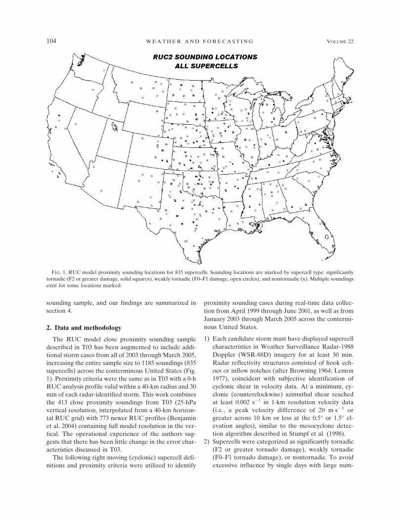
FIG. 1. RUC model proximity sounding locations for 835 supercells. Sounding locations are marked by supercell type: significantlytornadic (F2 or greater damage, solid squares), weakly tornadic (F0–F1 damage, open circles), and nontornadic (x). Multiple soundingsexist for some locations marked.


bers of supercells, not every supercell was includedin our dataset. Instead, we collected an average ofroughly two cases for each day when supercells oc-curred. When multiple supercells of the same typeoccurred within a single day, only those separatedby at least 3 h and 185 km became part of ourdataset. Additionally, proximity soundings were col-lected for storms that displayed “marginal” super-cell characteristics (i.e., peak cyclonic azimuthalshear less than 0.002 s�1), as well as discrete stormswith no supercell characteristics.

A RUC-2 analysis gridpoint sounding was generatedfor each 1999–2001 supercell at the analysis time closestto the most intense tornadoes with the tornadic super-cells, or the time of the most significant severe weatherreports with the nontornadic supercells, or at the timeof the most pronounced radar signatures if no severeweather was reported. In a slight change from the T03methodology, we collected soundings for both the ini-tiation (within the first hour of development) and ma-ture (�2 h after initiation) phases of supercells, as de-scribed in Edwards et al. (2004). However, to remainconsistent with T03, we considered only a single maturephase sounding for each storm case, or an initiationsounding if no mature phase sounding was available fora particular storm.

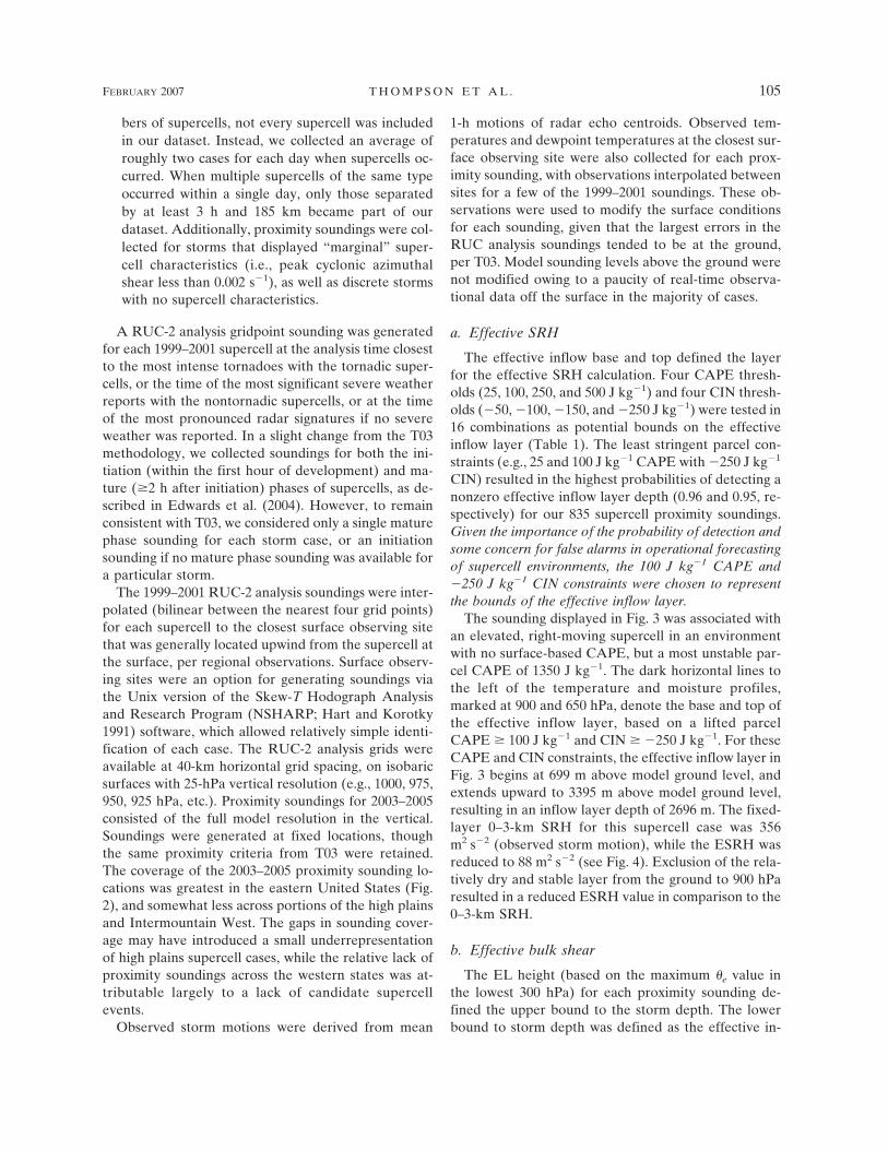
The 1999–2001 RUC-2 analysis soundings were inter-polated (bilinear between the nearest four grid points)for each supercell to the closest surface observing sitethat was generally located upwind from the supercell atthe surface, per regional observations. Surface observ-ing sites were an option for generating soundings viathe Unix version of the Skew-T Hodograph Analysisand Research Program (NSHARP; Hart and Korotky1991) software, which allowed relatively simple identi-fication of each case. The RUC-2 analysis grids wereavailable at 40-km horizontal grid spacing, on isobaricsurfaces with 25-hPa vertical resolution (e.g., 1000, 975,950, 925 hPa, etc.). Proximity soundings for 2003–2005consisted of the full model resolution in the vertical.Soundings were generated at fixed locations, thoughthe same proximity criteria from T03 were retained.The coverage of the 2003–2005 proximity sounding lo-cations was greatest in the eastern United States (Fig.2), and somewhat less across portions of the high plainsand Intermountain West. The gaps in sounding cover-age may have introduced a small underrepresentationof high plains supercell cases, while the relative lack ofproximity soundings across the western states was at-tributable largely to a lack of candidate supercellevents.

Observed storm motions were derived from mean

1-h motions of radar echo centroids. Observed tem-peratures and dewpoint temperatures at the closest sur-face observing site were also collected for each prox-imity sounding, with observations interpolated betweensites for a few of the 1999–2001 soundings. These ob-servations were used to modify the surface conditionsfor each sounding, given that the largest errors in theRUC analysis soundings tended to be at the ground,per T03. Model sounding levels above the ground werenot modified owing to a paucity of real-time observa-tional data off the surface in the majority of cases.

a. Effective SRH

The effective inflow base and top defined the layerfor the effective SRH calculation. Four CAPE thresh-olds (25, 100, 250, and 500 J kg�1) and four CIN thresh-olds (�50, �100, �150, and �250 J kg�1) were tested in16 combinations as potential bounds on the effectiveinflow layer (Table 1). The least stringent parcel con-straints (e.g., 25 and 100 J kg�1 CAPE with �250 J kg�1

CIN) resulted in the highest probabilities of detecting anonzero effective inflow layer depth (0.96 and 0.95, re-spectively) for our 835 supercell proximity soundings.Given the importance of the probability of detection andsome concern for false alarms in operational forecastingof supercell environments, the 100 J kg�1 CAPE and�250 J kg�1 CIN constraints were chosen to representthe bounds of the effective inflow layer.

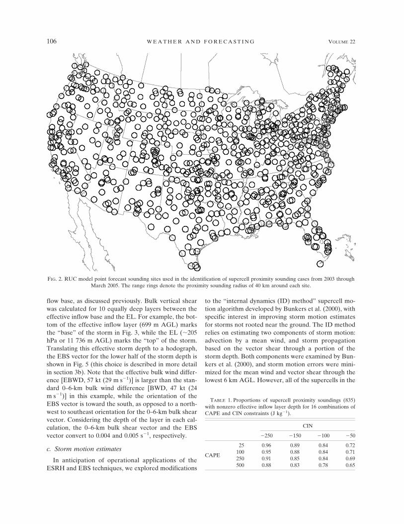
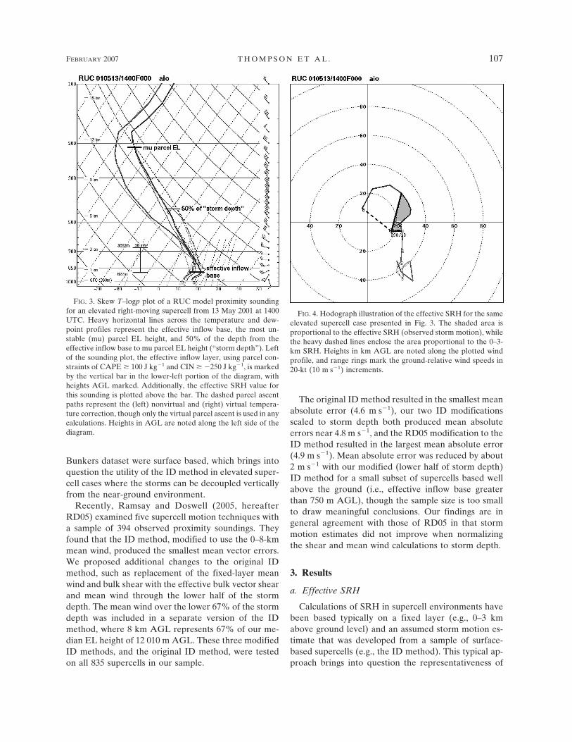
The sounding displayed in Fig. 3 was associated withan elevated, right-moving supercell in an environmentwith no surface-based CAPE, but a most unstable par-cel CAPE of 1350 J kg�1. The dark horizontal lines tothe left of the temperature and moisture profiles,marked at 900 and 650 hPa, denote the base and top ofthe effective inflow layer, based on a lifted parcelCAPE � 100 J kg�1 and CIN � �250 J kg�1. For theseCAPE and CIN constraints, the effective inflow layer inFig. 3 begins at 699 m above model ground level, andextends upward to 3395 m above model ground level,resulting in an inflow layer depth of 2696 m. The fixed-layer 0–3-km SRH for this supercell case was 356m2 s�2 (observed storm motion), while the ESRH wasreduced to 88 m2 s�2 (see Fig. 4). Exclusion of the rela-tively dry and stable layer from the ground to 900 hParesulted in a reduced ESRH value in comparison to the0–3-km SRH.

b. Effective bulk shear

The EL height (based on the maximum �e value inthe lowest 300 hPa) for each proximity sounding de-fined the upper bound to the storm depth. The lowerbound to storm depth was defined as the effective in-


flow base, as discussed previously. Bulk vertical shearwas calculated for 10 equally deep layers between theeffective inflow base and the EL. For example, the bot-tom of the effective inflow layer (699 m AGL) marksthe “base” of the storm in Fig. 3, while the EL (�205hPa or 11 736 m AGL) marks the “top” of the storm.Translating this effective storm depth to a hodograph,the EBS vector for the lower half of the storm depth isshown in Fig. 5 (this choice is described in more detailin section 3b). Note that the effective bulk wind differ-ence [EBWD, 57 kt (29 m s�1)] is larger than the stan-dard 0–6-km bulk wind difference [BWD, 47 kt (24m s�1)] in this example, while the orientation of theEBS vector is toward the south, as opposed to a north-west to southeast orientation for the 0–6-km bulk shearvector. Considering the depth of the layer in each cal-culation, the 0–6-km bulk shear vector and the EBSvector convert to 0.004 and 0.005 s�1, respectively.

c. Storm motion estimates

In anticipation of operational applications of theESRH and EBS techniques, we explored modifications

to the “internal dynamics (ID) method” supercell mo-tion algorithm developed by Bunkers et al. (2000), withspecific interest in improving storm motion estimatesfor storms not rooted near the ground. The ID methodrelies on estimating two components of storm motion:advection by a mean wind, and storm propagationbased on the vector shear through a portion of thestorm depth. Both components were examined by Bun-kers et al. (2000), and storm motion errors were mini-mized for the mean wind and vector shear through thelowest 6 km AGL. However, all of the supercells in the

TABLE 1. Proportions of supercell proximity soundings (835)with nonzero effective inflow layer depth for 16 combinations ofCAPE and CIN constraints (J kg�1).

CIN

�250 �150 �100 �50

CAPE

25 0.96 0.89 0.84 0.72100 0.95 0.88 0.84 0.71250 0.91 0.85 0.84 0.69500 0.88 0.83 0.78 0.65

FIG. 2. RUC model point forecast sounding sites used in the identification of supercell proximity sounding cases from 2003 throughMarch 2005. The range rings denote the proximity sounding radius of 40 km around each site.


Bunkers dataset were surface based, which brings intoquestion the utility of the ID method in elevated super-cell cases where the storms can be decoupled verticallyfrom the near-ground environment.

Recently, Ramsay and Doswell (2005, hereafterRD05) examined five supercell motion techniques witha sample of 394 observed proximity soundings. Theyfound that the ID method, modified to use the 0–8-kmmean wind, produced the smallest mean vector errors.We proposed additional changes to the original IDmethod, such as replacement of the fixed-layer meanwind and bulk shear with the effective bulk vector shearand mean wind through the lower half of the stormdepth. The mean wind over the lower 67% of the stormdepth was included in a separate version of the IDmethod, where 8 km AGL represents 67% of our me-dian EL height of 12 010 m AGL. These three modifiedID methods, and the original ID method, were testedon all 835 supercells in our sample.

The original ID method resulted in the smallest meanabsolute error (4.6 m s�1), our two ID modificationsscaled to storm depth both produced mean absoluteerrors near 4.8 m s�1, and the RD05 modification to theID method resulted in the largest mean absolute error(4.9 m s�1). Mean absolute error was reduced by about2 m s�1 with our modified (lower half of storm depth)ID method for a small subset of supercells based wellabove the ground (i.e., effective inflow base greaterthan 750 m AGL), though the sample size is too smallto draw meaningful conclusions. Our findings are ingeneral agreement with those of RD05 in that stormmotion estimates did not improve when normalizingthe shear and mean wind calculations to storm depth.

3. Results

a. Effective SRH

Calculations of SRH in supercell environments havebeen based typically on a fixed layer (e.g., 0–3 kmabove ground level) and an assumed storm motion es-timate that was developed from a sample of surface-based supercells (e.g., the ID method). This typical ap-proach brings into question the representativeness of

FIG. 3. Skew T–logp plot of a RUC model proximity soundingfor an elevated right-moving supercell from 13 May 2001 at 1400UTC. Heavy horizontal lines across the temperature and dew-point profiles represent the effective inflow base, the most un-stable (mu) parcel EL height, and 50% of the depth from theeffective inflow base to mu parcel EL height (“storm depth”). Leftof the sounding plot, the effective inflow layer, using parcel con-straints of CAPE � 100 J kg�1 and CIN � �250 J kg�1, is markedby the vertical bar in the lower-left portion of the diagram, withheights AGL marked. Additionally, the effective SRH value forthis sounding is plotted above the bar. The dashed parcel ascentpaths represent the (left) nonvirtual and (right) virtual tempera-ture correction, though only the virtual parcel ascent is used in anycalculations. Heights in AGL are noted along the left side of thediagram.

FIG. 4. Hodograph illustration of the effective SRH for the sameelevated supercell case presented in Fig. 3. The shaded area isproportional to the effective SRH (observed storm motion), whilethe heavy dashed lines enclose the area proportional to the 0–3-km SRH. Heights in km AGL are noted along the plotted windprofile, and range rings mark the ground-relative wind speeds in20-kt (10 m s�1) increments.


0–1 or 0–3 km as the “inflow” layer for most supercells,particularly in the special case of an elevated supercell.SRH is likely overestimated for elevated storms by in-cluding vertical shear in the near-ground layer that isdecoupled vertically from the storm (e.g., instabilitybased above a stable surface layer, as shown in Fig. 3).

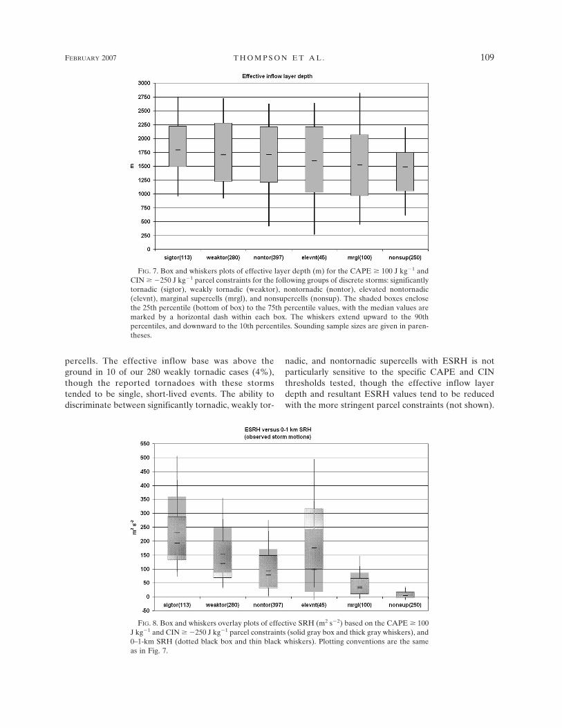
The most obvious elevated supercell environmentcan be defined as an effective inflow base above theground. However, there are cases where a supercell canbe considered somewhat elevated when the most un-stable parcel originates above the ground, but the ef-fective inflow base is the ground level (Fig. 6). Thissituation is similar to the “large CIN–high level of freeconvection (LFC)” environments discussed by Davies(2004). Here, a supercell is defined as elevated whenthe effective inflow base is above the ground in theassociated proximity sounding.

It is important to note that in some cases an effectiveinflow layer was not identified; thus, ESRH could notbe calculated and was assumed to be zero. An effectiveinflow layer can be missing from a sounding for thefollowing reasons:

1) insufficient buoyancy (CAPE � 100 J kg�1 for alllifted parcels),

2) excessive convective inhibition (CIN � �250 for alllifted parcels), or

3) the effective inflow “layer” is a single level in thesounding. This scenario is often associated withmodifying the RUC sounding for the observed sur-face conditions, while the cool and dry biases in theRUC analyses result in the next level above theground not meeting the effective inflow layer con-straints.

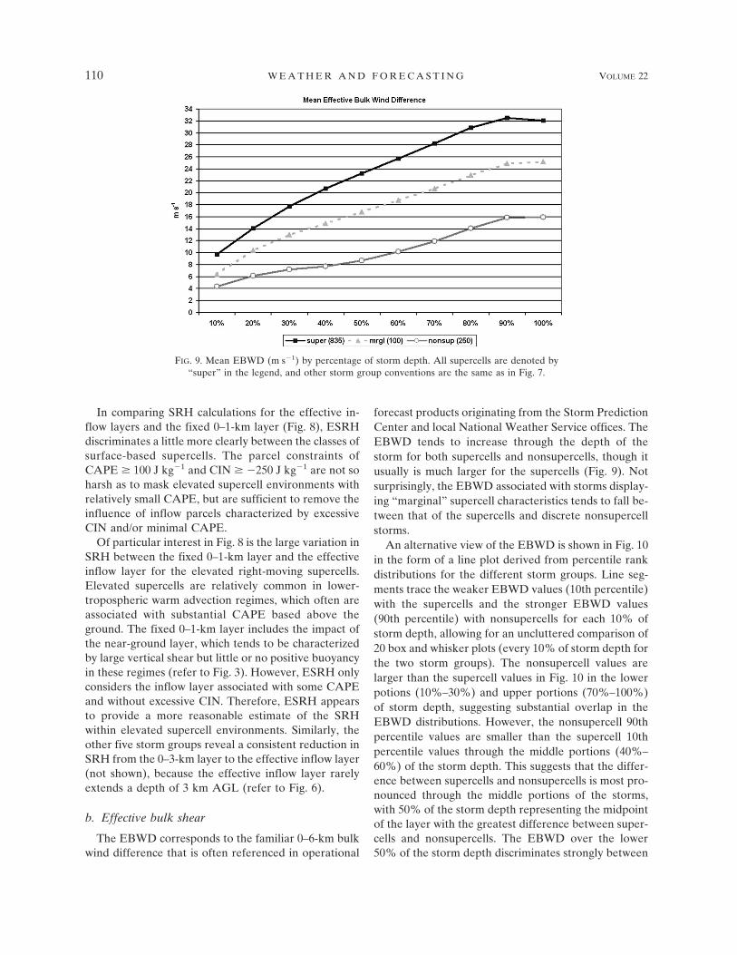
Figure 7 suggests that the depth of the effective in-flow layer varies little across a spectrum of storm types,though the elevated right-moving supercells are associ-ated with somewhat shallower inflow layers in the caseswith lesser CAPE (e.g., the lowest quartile in Fig. 7 forthe elevated nontornadic supercells). Interestingly, ef-fective layer depths (which begin at the ground for allbut 10 weakly tornadic supercells and 45 elevated non-tornadic supercells) were typically between the stan-dard 0–1- and 0–3-km SRH layers. Effective inflowlayer depths with the elevated nontornadic supercellswere similar to those with the surface-based nontor-nadic supercells, though effective inflow bases rangedfrom just above the ground to in excess of 2 km AGL inthe elevated cases.

ESRH decreases markedly from the significantly tor-nadic supercells to the nontornadic supercells (Fig. 8),while the ESRH with elevated nontornadic supercellsresembles the values associated with nontornadic su-

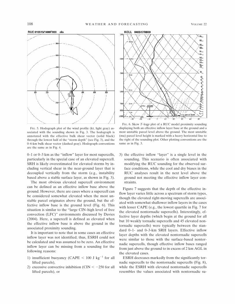
FIG. 5. Hodograph plot of the wind profile (kt, light gray) as-sociated with the sounding shown in Fig. 3. The hodograph isannotated with the effective bulk shear vector (solid black)through the lowest half of the “storm depth” (see Fig. 3), and the0–6-km bulk shear vector (dashed gray). Hodograph conventionsare the same as in Fig. 4.

FIG. 6. Skew T–logp plot of a RUC model proximity soundingdisplaying both an effective inflow layer base at the ground and amost unstable parcel level above the ground. The most unstable(mu) parcel level height is marked with a heavy horizontal line tothe right of the sounding plot. Other plotting conventions are thesame as in Fig. 3.


percells. The effective inflow base was above theground in 10 of our 280 weakly tornadic cases (4%),though the reported tornadoes with these stormstended to be single, short-lived events. The ability todiscriminate between significantly tornadic, weakly tor-

nadic, and nontornadic supercells with ESRH is notparticularly sensitive to the specific CAPE and CINthresholds tested, though the effective inflow layerdepth and resultant ESRH values tend to be reducedwith the more stringent parcel constraints (not shown).

FIG. 8. Box and whiskers overlay plots of effective SRH (m2 s�2) based on the CAPE � 100J kg�1 and CIN � �250 J kg�1 parcel constraints (solid gray box and thick gray whiskers), and0–1-km SRH (dotted black box and thin black whiskers). Plotting conventions are the sameas in Fig. 7.

FIG. 7. Box and whiskers plots of effective layer depth (m) for the CAPE � 100 J kg�1 andCIN � �250 J kg�1 parcel constraints for the following groups of discrete storms: significantlytornadic (sigtor), weakly tornadic (weaktor), nontornadic (nontor), elevated nontornadic(elevnt), marginal supercells (mrgl), and nonsupercells (nonsup). The shaded boxes enclosethe 25th percentile (bottom of box) to the 75th percentile values, with the median values aremarked by a horizontal dash within each box. The whiskers extend upward to the 90thpercentiles, and downward to the 10th percentiles. Sounding sample sizes are given in paren-theses.


In comparing SRH calculations for the effective in-flow layers and the fixed 0–1-km layer (Fig. 8), ESRHdiscriminates a little more clearly between the classes ofsurface-based supercells. The parcel constraints ofCAPE � 100 J kg�1 and CIN � �250 J kg�1 are not soharsh as to mask elevated supercell environments withrelatively small CAPE, but are sufficient to remove theinfluence of inflow parcels characterized by excessiveCIN and/or minimal CAPE.

Of particular interest in Fig. 8 is the large variation inSRH between the fixed 0–1-km layer and the effectiveinflow layer for the elevated right-moving supercells.Elevated supercells are relatively common in lower-tropospheric warm advection regimes, which often areassociated with substantial CAPE based above theground. The fixed 0–1-km layer includes the impact ofthe near-ground layer, which tends to be characterizedby large vertical shear but little or no positive buoyancyin these regimes (refer to Fig. 3). However, ESRH onlyconsiders the inflow layer associated with some CAPEand without excessive CIN. Therefore, ESRH appearsto provide a more reasonable estimate of the SRHwithin elevated supercell environments. Similarly, theother five storm groups reveal a consistent reduction inSRH from the 0–3-km layer to the effective inflow layer(not shown), because the effective inflow layer rarelyextends a depth of 3 km AGL (refer to Fig. 6).

b. Effective bulk shear

The EBWD corresponds to the familiar 0–6-km bulkwind difference that is often referenced in operational

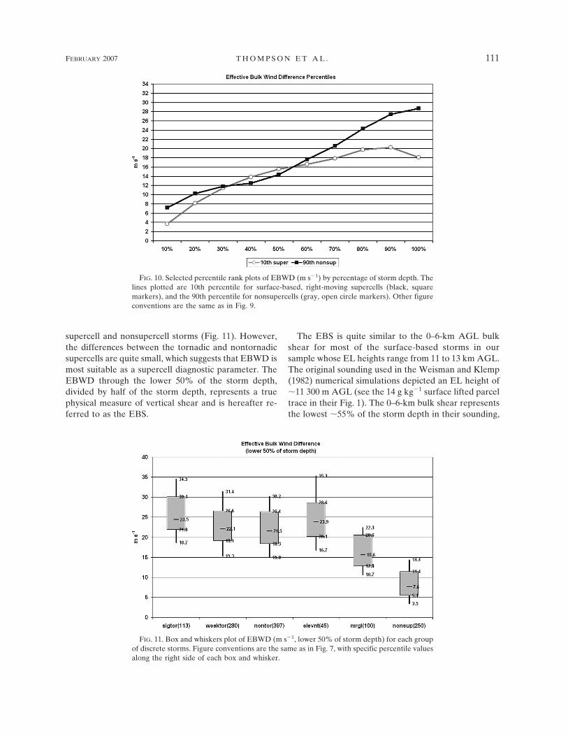
forecast products originating from the Storm PredictionCenter and local National Weather Service offices. TheEBWD tends to increase through the depth of thestorm for both supercells and nonsupercells, though itusually is much larger for the supercells (Fig. 9). Notsurprisingly, the EBWD associated with storms display-ing “marginal” supercell characteristics tends to fall be-tween that of the supercells and discrete nonsupercellstorms.

An alternative view of the EBWD is shown in Fig. 10in the form of a line plot derived from percentile rankdistributions for the different storm groups. Line seg-ments trace the weaker EBWD values (10th percentile)with the supercells and the stronger EBWD values(90th percentile) with nonsupercells for each 10% ofstorm depth, allowing for an uncluttered comparison of20 box and whisker plots (every 10% of storm depth forthe two storm groups). The nonsupercell values arelarger than the supercell values in Fig. 10 in the lowerpotions (10%–30%) and upper portions (70%–100%)of storm depth, suggesting substantial overlap in theEBWD distributions. However, the nonsupercell 90thpercentile values are smaller than the supercell 10thpercentile values through the middle portions (40%–60%) of the storm depth. This suggests that the differ-ence between supercells and nonsupercells is most pro-nounced through the middle portions of the storms,with 50% of the storm depth representing the midpointof the layer with the greatest difference between super-cells and nonsupercells. The EBWD over the lower50% of the storm depth discriminates strongly between

FIG. 9. Mean EBWD (m s�1) by percentage of storm depth. All supercells are denoted by“super” in the legend, and other storm group conventions are the same as in Fig. 7.


supercell and nonsupercell storms (Fig. 11). However,the differences between the tornadic and nontornadicsupercells are quite small, which suggests that EBWD ismost suitable as a supercell diagnostic parameter. TheEBWD through the lower 50% of the storm depth,divided by half of the storm depth, represents a truephysical measure of vertical shear and is hereafter re-ferred to as the EBS.

The EBS is quite similar to the 0–6-km AGL bulkshear for most of the surface-based storms in oursample whose EL heights range from 11 to 13 km AGL.The original sounding used in the Weisman and Klemp(1982) numerical simulations depicted an EL height of�11 300 m AGL (see the 14 g kg�1 surface lifted parceltrace in their Fig. 1). The 0–6-km bulk shear representsthe lowest �55% of the storm depth in their sounding,

FIG. 10. Selected percentile rank plots of EBWD (m s�1) by percentage of storm depth. Thelines plotted are 10th percentile for surface-based, right-moving supercells (black, squaremarkers), and the 90th percentile for nonsupercells (gray, open circle markers). Other figureconventions are the same as in Fig. 9.

FIG. 11. Box and whiskers plot of EBWD (m s�1, lower 50% of storm depth) for each groupof discrete storms. Figure conventions are the same as in Fig. 7, with specific percentile valuesalong the right side of each box and whisker.


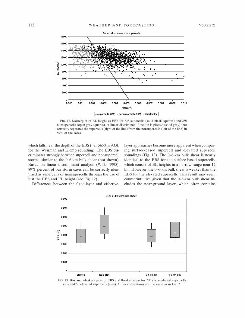
which falls near the depth of the EBS (i.e., 5650 m AGLfor the Weisman and Klemp sounding). The EBS dis-criminates strongly between supercell and nonsupercellstorms, similar to the 0–6-km bulk shear (not shown).Based on linear discriminant analysis (Wilks 1995),89% percent of our storm cases can be correctly iden-tified as supercells or nonsupercells through the use ofjust the EBS and EL height (see Fig. 12).

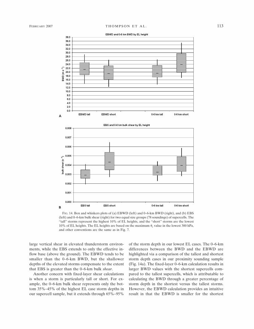
Differences between the fixed-layer and effective-

layer approaches become more apparent when compar-ing surface-based supercell and elevated supercellsoundings (Fig. 13). The 0–6-km bulk shear is nearlyidentical to the EBS for the surface-based supercells,which consist of EL heights in a narrow range near 12km. However, the 0–6-km bulk shear is weaker than theEBS for the elevated supercells. This result may seemcounterintuitive given that the 0–6-km bulk shear in-cludes the near-ground layer, which often contains

FIG. 12. Scatterplot of EL height vs EBS for 835 supercells (solid black squares) and 250nonsupercells (open gray squares). A linear discriminant function is plotted (solid gray) thatcorrectly separates the supercells (right of the line) from the nonsupercells (left of the line) in89% of the cases.

FIG. 13. Box and whiskers plots of EBS and 0–6-km shear for 780 surface-based supercells(sb) and 55 elevated supercells (elev). Other conventions are the same as in Fig. 7.


large vertical shear in elevated thunderstorm environ-ments, while the EBS extends to only the effective in-flow base (above the ground). The EBWD tends to besmaller than the 0–6-km BWD, but the shallowerdepths of the elevated storms compensate to the extentthat EBS is greater than the 0–6-km bulk shear.

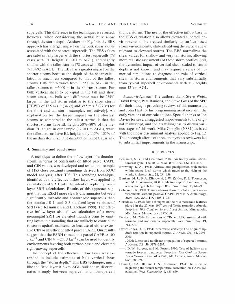
Another concern with fixed-layer shear calculationsis when a storm is particularly tall or short. For ex-ample, the 0–6-km bulk shear represents only the bot-tom 35%–45% of the highest EL case storm depths inour supercell sample, but it extends through 65%–95%

of the storm depth in our lowest EL cases. The 0–6-kmdifferences between the BWD and the EBWD arehighlighted via a comparison of the tallest and shorteststorm depth cases in our proximity sounding sample(Fig. 14a). The fixed-layer 0–6-km calculation results inlarger BWD values with the shortest supercells com-pared to the tallest supercells, which is attributable tocalculating the BWD through a greater percentage ofstorm depth in the shortest versus the tallest storms.However, the EBWD calculation provides an intuitiveresult in that the EBWD is smaller for the shortest

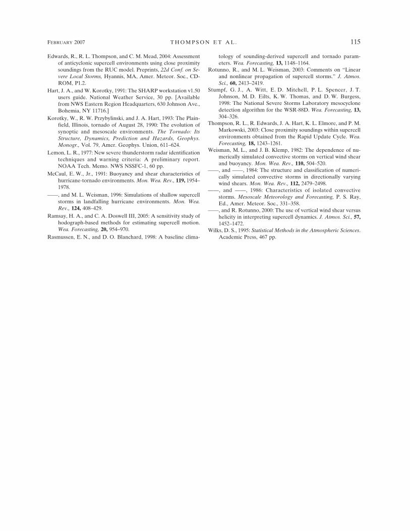
FIG. 14. Box and whiskers plots of (a) EBWD (left) and 0–6-km BWD (right), and (b) EBS(left) and 0–6-km bulk shear (right) for two equal size groups (78 soundings) of supercells. The“tall” storms represent the highest 10% of EL heights, and the “short” storms are the lowest10% of EL heights. The EL heights are based on the maximum �e value in the lowest 300 hPa,and other conventions are the same as in Fig. 7.


supercells. This difference in the techniques is reversed,however, when considering the actual bulk shearthrough the storm depth. As shown in Fig. 14b, the EBSapproach has a larger impact on the bulk shear valuesassociated with the shortest supercells. The EBS valuesare substantially larger with the shortest supercells (78cases with EL heights � 9903 m AGL), and slightlysmaller with the tallest storms (78 cases with EL heights� 13 892 m AGL). The EBS has a greater impact on theshorter storms because the depth of the shear calcu-lation is much less compared to that of the talleststorms. EBS depth varies from �7900 m AGL in thetallest storms to �3000 m in the shortest storms. Forbulk vertical shear to be equal in the tall and shortstorm cases, the bulk wind difference must be 225%larger in the tall storm relative to the short storm[EBWD of 17.5 m s�1 (34 kt) and 39.5 m s�1 (77 kt) forthe short and tall storm examples, respectively]. Anexplanation for the larger impact on the shorteststorms, as compared to the tallest storms, is that theshortest storms have EL heights 50%–80% of the me-dian EL height in our sample (12 011 m AGL), whilethe tallest storms have EL heights only 115%–135% ofthe median storm (i.e., the distribution is not Gaussian).

4. Summary and conclusions

A technique to define the inflow layer of a thunder-storm, in terms of constraints on lifted parcel CAPEand CIN values, was developed and tested on a sampleof 1185 close proximity soundings derived from RUCmodel analyses, after T03. This sounding technique,identified as the effective inflow layer, was applied tocalculations of SRH with the intent of replacing fixed-layer SRH calculations. Results of this approach sug-gest that the ESRH more clearly discriminates betweensignificantly tornadic and nontornadic supercells thanthe standard 0–1- and 0–3-km fixed-layer versions ofSRH (see Rasmussen and Blanchard 1998). The effec-tive inflow layer also allows calculation of a moremeaningful SRH for elevated thunderstorms by omit-ting layers in a sounding that are unlikely to contributeto storm updraft maintenance because of either exces-sive CIN or insufficient lifted parcel CAPE. Our resultssuggest that the ESRH (based on a parcel CAPE � 100J kg�1 and CIN � �250 J kg�1) can be used to identifyenvironments favoring both surface-based and elevatedright-moving supercells.

The concept of the effective inflow layer was ex-tended to include estimates of bulk vertical shearthrough the “storm depth.” This EBS technique, muchlike the fixed-layer 0–6-km AGL bulk shear, discrimi-nates strongly between supercell and nonsupercell

thunderstorms. The use of the effective inflow base inthe EBS calculation also allows elevated supercell en-vironments to be treated similarly to surface-basedstorm environments, while identifying the vertical shearrelevant to elevated storms. The EBS normalizes theshear values for shallow and very tall storms, allowingmore realistic assessments of these storm profiles. Still,the dynamical impact of vertical shear scaled to stormdepth is not known, and may require a series of nu-merical simulations to diagnose the role of verticalshear in storm environments that vary substantiallyfrom typical supercell environments with EL heightsnear 12 km AGL.

Acknowledgments. The authors thank Steve Weiss,David Bright, Pete Banacos, and Steve Goss of the SPCfor their thought-provoking reviews of this manuscript,and John Hart for his programming assistance with theearly versions of our calculations. Special thanks to JonDavies for several suggested improvements to the origi-nal manuscript, and for his willingness to discuss vari-ous stages of this work. Mike Coniglio (NSSL) assistedwith the linear discriminant analysis applied to Fig. 12.The thorough efforts of three anonymous reviewers ledto substantial improvements in the manuscript.

REFERENCES

Benjamin, S. G., and Coauthors, 2004: An hourly assimilation–forecast cycle: The RUC. Mon. Wea. Rev., 132, 495–518.

Browning, K. A., 1964: Airflow and precipitation trajectorieswithin severe local storms which travel to the right of thewinds. J. Atmos. Sci., 21, 634–639.

Bunkers, M. J., B. A. Klimowski, J. W. Zeitler, R. L. Thompson,and M. L. Weisman, 2000: Predicting supercell motion usinga new hodograph technique. Wea. Forecasting, 15, 61–79.

Colman, B. R., 1990: Thunderstorms above frontal surfaces in en-vironments without positive CAPE. Part I: A climatology.Mon. Wea. Rev., 118, 1103–1122.

Corfidi, S. F., 1998: Some thoughts on the role mesoscale featuresplayed in the 27 May 1997 central Texas tornado outbreak.Preprints, 19th Conf. on Severe Local Storms, Minneapolis,MN, Amer. Meteor. Soc., 177–180.

Davies, J. M., 2004: Estimations of CIN and LFC associated withtornadic and nontornadic supercells. Wea. Forecasting, 19,714–726.

Davies-Jones, R. P., 1984: Streamwise vorticity: The origin of up-draft rotation in supercell storms. J. Atmos. Sci., 41, 2991–3006.

——, 2002: Linear and nonlinear propagation of supercell storms.J. Atmos. Sci., 59, 3178–3205.

——, D. W. Burgess, and M. Foster, 1990: Test of helicity as atornado forecast parameter. Preprints, 16th Conf. on SevereLocal Storms, Kananaskis Park, AB, Canada, Amer. Meteor.Soc., 588–592.

Doswell, C. A., III, and E. N. Rasmussen, 1994: The effect ofneglecting the virtual temperature correction on CAPE cal-culations. Wea. Forecasting, 9, 625–629.


Edwards, R., R. L. Thompson, and C. M. Mead, 2004: Assessmentof anticyclonic supercell environments using close proximitysoundings from the RUC model. Preprints, 22d Conf. on Se-vere Local Storms, Hyannis, MA, Amer. Meteor. Soc., CD-ROM, P1.2.

Hart, J. A., and W. Korotky, 1991: The SHARP workstation v1.50users guide. National Weather Service, 30 pp. [Availablefrom NWS Eastern Region Headquarters, 630 Johnson Ave.,Bohemia, NY 11716.]

Korotky, W., R. W. Przybylinski, and J. A. Hart, 1993: The Plain-field, Illinois, tornado of August 28, 1990: The evolution ofsynoptic and mesoscale environments. The Tornado: ItsStructure, Dynamics, Prediction and Hazards, Geophys.Monogr., Vol. 79, Amer. Geophys. Union, 611–624.

Lemon, L. R., 1977: New severe thunderstorm radar identificationtechniques and warning criteria: A preliminary report.NOAA Tech. Memo. NWS NSSFC-1, 60 pp.

McCaul, E. W., Jr., 1991: Buoyancy and shear characteristics ofhurricane-tornado environments. Mon. Wea. Rev., 119, 1954–1978.

——, and M. L. Weisman, 1996: Simulations of shallow supercellstorms in landfalling hurricane environments. Mon. Wea.Rev., 124, 408–429.

Ramsay, H. A., and C. A. Doswell III, 2005: A sensitivity study ofhodograph-based methods for estimating supercell motion.Wea. Forecasting, 20, 954–970.

Rasmussen, E. N., and D. O. Blanchard, 1998: A baseline clima-

tology of sounding-derived supercell and tornado param-eters. Wea. Forecasting, 13, 1148–1164.

Rotunno, R., and M. L. Weisman, 2003: Comments on “Linearand nonlinear propagation of supercell storms.” J. Atmos.Sci., 60, 2413–2419.

Stumpf, G. J., A. Witt, E. D. Mitchell, P. L. Spencer, J. T.Johnson, M. D. Eilts, K. W. Thomas, and D. W. Burgess,1998: The National Severe Storms Laboratory mesocyclonedetection algorithm for the WSR-88D. Wea. Forecasting, 13,304–326.

Thompson, R. L., R. Edwards, J. A. Hart, K. L. Elmore, and P. M.Markowski, 2003: Close proximity soundings within supercellenvironments obtained from the Rapid Update Cycle. Wea.Forecasting, 18, 1243–1261.

Weisman, M. L., and J. B. Klemp, 1982: The dependence of nu-merically simulated convective storms on vertical wind shearand buoyancy. Mon. Wea. Rev., 110, 504–520.

——, and ——, 1984: The structure and classification of numeri-cally simulated convective storms in directionally varyingwind shears. Mon. Wea. Rev., 112, 2479–2498.

——, and ——, 1986: Characteristics of isolated convectivestorms. Mesoscale Meteorology and Forecasting, P. S. Ray,Ed., Amer. Meteor. Soc., 331–358.

——, and R. Rotunno, 2000: The use of vertical wind shear versushelicity in interpreting supercell dynamics. J. Atmos. Sci., 57,1452–1472.

Wilks, D. S., 1995: Statistical Methods in the Atmospheric Sciences.Academic Press, 467 pp.


Documents

Effective Storm-Relative Helicity and Bulk Shear in ... · Effective Storm-Relative Helicity and Bulk Shear in Supercell Thunderstorm Environments RICHARD L. THOMPSON,COREY M. MEAD,