Embed Size (px)
Citation preview

Iterative Methods for Solving Linear Systems of Equations
(part of the course given for the 2nd grade at BGU,
ME)

Iterative Methods
And generate the sequence of approximation by
This procedure is similar to the fixed point method.
An iterative technique to solve Ax=b starts with an initial approximation and generates a sequence)0(x 0
)(k
kx
First we convert the system Ax=b into an equivalent formcTxx
...3,2,1 ,)1()( kkk cTxx
The stopping criterion:
)(
)1()(
k
kk
x
xx

Iterative Methods (Example)
51 8 3 :
11 10 2 :
52 3 11 :
6 2 10 :
4324
43213
43212
3211
xxxE
xxxxE
xxxxE
xxxE
We rewrite the system in the x=Tx+c form
8
51
8
1
8
3
10
11
10
1
10
1
5
1-
11
52
11
3
11
1
11
1
5
3
5
1
10
1
324
4213
4312
321
xxx
xxxx
xxxx
xxx

Iterative Methods (Example) – cont.
1.8750 8
51
8
1
8
3-
1000.110
11
10
1
10
1
5
1-
2727.2 11
52
11
3 -
11
1
11
1
6000.0 5
3
5
1
10
1
)0(3
)0(2
)1(4
)0(4
)0(2
)0(1
)1(3
)0(4
)0(3
)0(1
)1(2
)0(3
)0(2
)1(1
xxx
xxxx
xxxx
xxx
and start iterations with
)0 ,0 ,0 ,0()0( x
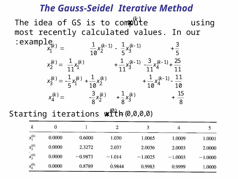
Continuing the iterations, the results are in the Table:

The Jacobi Iterative Method
The method of the Example is called the Jacobi iterative method
ni
a
bxa
xii
ijj
ikjij
ki ,....,2 ,1 ,
1
)1(
)(

Algorithm: Jacobi Iterative Method

The Jacobi Method: x=Tx+c Form
nnnn
n
n
aaa
aaa
aaa
. . .
. . .
21
22221
11211
A
ULD
0................... .....0
. ......................
.............................
................ 0
........ 0
0 .....
...........................
..........................
.........0..........
...0.......... ............. 0
..0...............0
.......0....................
............................
...0.......... 0
.....0..........0
n1,-n
2
112
1,1
2122
11
a
a
aa
aa
a
a
a
a
n
n
nnnnn
ULDA

The Jacobi Method: x=Tx+c Form (cont)
ULDA and the equation Ax=b can be transformed into
bxULD
bxULDx
bDxULDx 11
ULDT 1 bDc 1Finally
The Gauss-Seidel Iterative Method
8
51
8
1
8
3-
10
11
10
1
10
1
5
1-
11
52
11
3 -
11
1
11
1
5
3
5
1
10
1
)(3
)(2
)(4
)1(4
)(2
)(1
)(3
)1(4
)1(3
)(1
)(2
)1(3
)1(2
)(1
kkk
kkkk
kkkk
kkk
xxx
xxxx
xxxx
xxx
The idea of GS is to compute using most recently calculated values. In our example:
)(kx
Starting iterations with , we obtain
)0 ,0 ,0 ,0()0( x
The Gauss-Seidel Iterative Method
ni
a
bxaxa
xii
i
j
n
iji
kjij
kjij
ki ,....,2 ,1 ,
1
1 1
)1()(
)(
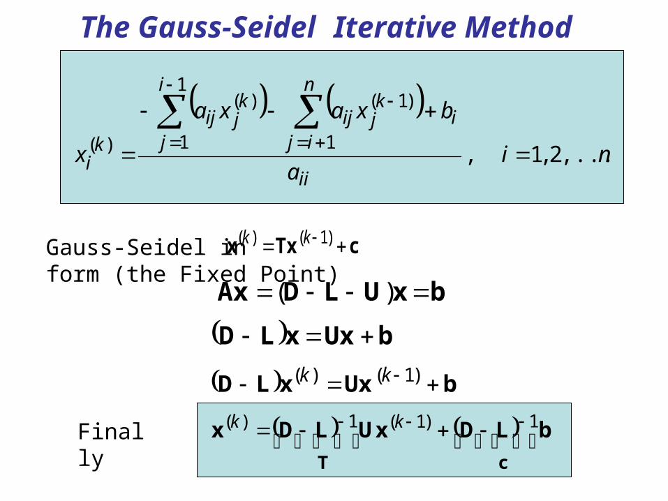
Gauss-Seidel in form (the Fixed Point)
cTxx )1()( kk
bUxxLD
bxULDAx )(
bUxxLD )1()( kk
cT
bLDxULDx 1)1(1)( kkFinally
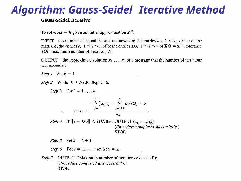
Algorithm: Gauss-Seidel Iterative Method
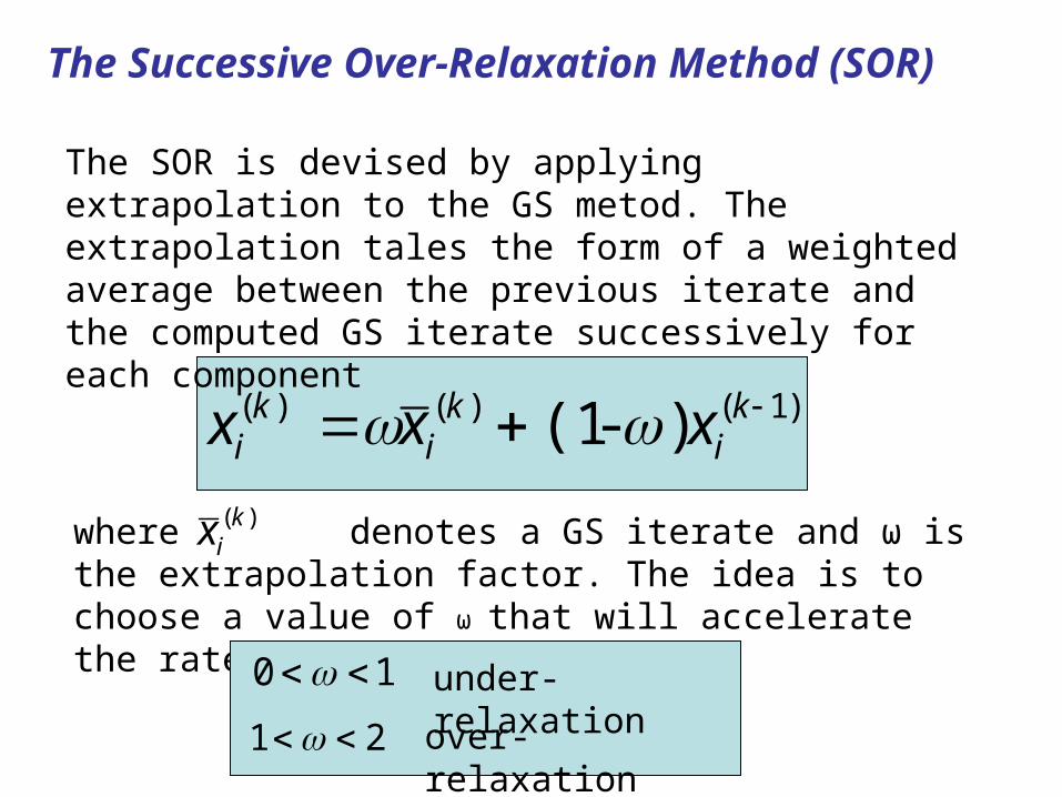
The Successive Over-Relaxation Method (SOR)
)1()()( )-(1 ki
ki
ki xxx
The SOR is devised by applying extrapolation to the GS metod. The extrapolation tales the form of a weighted average between the previous iterate and the computed GS iterate successively for each component
where denotes a GS iterate and ω is the extrapolation factor. The idea is to choose a value of ω that will accelerate the rate of convergence.
)(kix
10 under-relaxation21 over-relaxation

SOR: Example
244
30 4 3
42 3 4
32
321
21
xx
xxx
xx
Solution: x=(3, 4, -5)