Embed Size (px)
Citation preview
A new iterative method for solving a class of complexsymmetric system of linear equations
Davod Hezari · Davod Khojasteh Salkuyeh ·Vahid Edalatpour
Received: date / Accepted: date
Abstract We present a new stationary iterative method, called Scale-Splitting (SCSP) method,and investigate its convergence properties. The SCSP method naturally results in a simplematrix splitting preconditioner, called SCSP-preconditioner, for the original linear system.Some numerical comparisons are presented between the SCSP-preconditioner and severalavailable block preconditioners, such as PGSOR (Hezari et al. Numer. Linear Algebra Appl.22, 761-776, 2015) and rotate block triangular preconditioners (Bai, Sci. China Math. 56,2523-2538, 2013), when they are applied to expedite the convergence rate of Krylov subspaceiteration methods for solving the original complex system and its block real formulation,respectively. Numerical experiments show that the SCSP-preconditioner can compete withPGSOR-preconditioner and even more effective than the rotate block triangular precondi-tioners.
Keywords Complex symmetric linear systems · symmetric positive definite · preconditioner.
Mathematics Subject Classification (2000) 65F10 · 65F15.
1 Introduction
We consider the nonsingular system of linear equations of the form
Az = b, with A = W + iT, z = x+ iy and b = f + ig, (1)
where i =√−1 is the imaginary unit, the n× n matrices W and T are real and the vectors
x, y, f and g are all in Rn. Note that A is nonsingular if and only if null(W )∩null(T ) = 0and i is not a generalized eigenvalue of the matrix pair (W,T ) (i.e., Tx 6= iWx for any x 6= 0),where null(·) denotes the null space of the corresponding matrix.
Such systems appear in a variety of scientific computing and engineering applicationssuch as computational electrodynamic [1,2], FFT-based solution of certain time-dependentPDEs [3], structural dynamics [4], diffuse optical tomography [5], quantum mechanics [6] and
D. HezariFaculty of Mathematical Sciences, University of Guilan, Rasht, IranE-mail: [email protected], [email protected]
D.K. SalkuyehFaculty of Mathematical Sciences, University of Guilan, Rasht, IranE-mail: [email protected], [email protected]
V. EdalatpourFaculty of Mathematical Sciences, University of Guilan, Rasht, IranE-mail: [email protected]
2 D. Hezari, V. Edalatpour and D.K. Salkuyeh
molecular scattering [7]. For more applications of this class of complex symmetric systems see[8] and references therein.
Bai et al. in [9] described the Hermitian and skew-Hermitian splitting (HSS) method tosolve non-Hermitian positive definite system of linear equations. By modifying and precondi-tioning the HSS iteration method, Bai et al. [10,11] presented a preconditioned and modifiedHSS (PMHSS) iteration method for solving the complex linear system (1). Moreover, Lopsidedversion of the PMHSS method has been presented by Li et al. [12]. Additionly, there are alsoother solution techniques for solving complex symmetric linear system (1) which are extensionsof Krylov subspace methods. For example, the well-known conjugate orthogonal conjugategradient (COCG) [13], quasi-minimal residual (QMR) method [14], conjugate A-orthogonalconjugate residual (COCR) [15], symmetric complex bi-conjugate gradient (SCBiCG) method[16] and Quasi-minimal residual variants of the COCG and COCR methods [17].
To avoid the complex arithmetic and constructing efficient preconditioners, one can dealwith the 2n× 2n equivalent real formulation
Ru ≡(W −TT W
)(xy
)=
(fg
)≡ d; (2)
see [8,18,19]. In [18], the foregoing PMHSS method is accommodated to solve the block two-by-two linear system (2) using real arithmetics. The PMHSS methods naturally lead to matrixsplitting preconditioners, called PMHSS preconditioners, for coefficient matrices of (1) and(2) which have recently gained more attention; see [20,21]. When the matrices W and T aresymmetric positive semi-definite satisfying null(W )∩null(T ) = 0, the convergence analysisof these PMHSS methods and the spectral properties of the preconditioned matrix have beenpresented for linear systems (1) and (2); see [18,11]. Based on the PMHSS preconditioningmatrix, Bai in [22] proposed three rotated block triangular preconditioning matrices for blocktwo-by-two linear system (2) as follows
L(ω) =1√
ω2 + 1G
(ωW + T 0ωT −W ωW + T
), (3)
U(ω) =1√
ω2 + 1G
(ωW + T ωW − T
0 ωW + T
),
and
P (ω) =1√
ω2 + 1G
(ωW + T 0ωT −W ωW + T
)(ωW + T 0
0 ωW + T
)−1(ωW + T ωW − T
0 ωW + T
),
where G = 12
(I −II I
)is a block Givens rotation, I is the identity matrix and ω is a real
constant. The matrices L(ω), U(ω) and P (ω) are called the rotated block lower triangu-lar (RBLT), rotated block upper triangular (RBUT) and rotated block triangular product(RBTP) preconditioners, respectively. The rotated block triangular preconditioners can beapplied not only to the case that the matrices W and T are symmetric positive semi-definitebut also to case that either W or T is nonsymmetric. At each step of the rotated block trian-gular preconditioning processes, it is required to invert the matrix ωW + T exactly. To avoidthis problem, an inexact variant of the rotated block triangular preconditioners have beenproposed in [23], which use a nonsingular approximation of ωW +T , for example, incompleteCholesky factorization or incomplete LU factorization when the matrix ωW +T is symmetricpositive definite or nonsymmetric, respectively.
Based on the successive overrelaxation (SOR) method, recently Salkuyeh et al. [19] appliedthe generalized SOR (GSOR) to efficiently solve the block two-by-two linear system (2).After that, they proposed a preconditioned variant of the GSOR (PGSOR) method [24] andestablished conditions such that the PGSOR iteration method to be more effective than theGSOR iteration method.

A new iterative method for solving a class of complex symmetric system of linear equations 3
In this paper, a new stationary matrix splitting iteration method, called Scale-Splitting(SCSP), is presented to solve the original complex system (1) and convergence theory togetherwith the spectral properties of the corresponding preconditioned matrix are established. Theauthors in [24] have established the convergence analysis of the PGSOR method when both ofthe matrices W and T are symmetric positive semi-definite and at leat one of them is positivedefinite. Here, we weaken these conditions to the requirement that both of the matrices W andT are symmetric positive semi-definite satisfying null(W )∩null(T ) = 0. Also, the SCSP andPGSOR iteration methods naturally leads to a preconditioning matrix for the original complexlinear system (1) and the block two-by-two linear system (2), respectively. Applications ofthese two preconditioners involve solving linear subsystem with the coefficient matrix ωW+Tthat depends on the structures of matrices W and T , and can be exactly solved by theCholesky factorization or LU factorization. Moreover, similar to the inexact rotated blocktriangular preconditioners, an inexact variant of the SCSP and PGSOR preconditioners can beused by applying a nonsingular approximation of the matrix ωW+T , for example, incompleteCholesky factorization or incomplete LU factorization when the matrix ωW +T is symmetricpositive definite or nonsymmetric, respectively. Numerical experiments show that the Krylovsubspace methods such as GMRES [25] or its restarted variant GMRES(`) [25] incorporatedwith the exact or inexact SCSP and PGSOR preconditioners lead to rapid convergence andtend to outperform the exact or inexact rotated block triangular preconditioners.
Throughout this paper, we use (·)T and ‖ · ‖ to show the transpose and Euclidean normof either a vector or a matrix, and denote by ρ(·) the spectral radius of the correspondingmatrix.
The outline of this paper is as follows. In section 2 we describe the SCSP iteration methodfor solving the original complex system (1) and investigate its convergence properties as wellas extending the analysis to the preconditioned GMRES method. In Section 3 we present andanalyze the PGSOR iteration method for solving the block two-by-two linear system (2) anddiscuss the spectral properties of the corresponding preconditioned matrix. Section 4 presentssome numerical examples to show the effectiveness of the SCSP iteration method and tocompare the effectiveness of the SCSP, PGSOR and rotate block triangular preconditionersto accelerate Krylov subspace iteration methods such as GMRES or its restarted variantGMRES(`).
2 Scale-Splitting iteration method
In this section, we present the SCSP iteration method for solving the original complex system(1). Let ω be a real positive constant and the matrix ωW +T be nonsingular. By multiplyingthe complex number (ω − i) through both sides of the complex system (1) we obtain thefollowing equivalent system
Aωz = (ω − i)b, (4)
where Aω = (ωW + T ) + i(ωT −W ) in which i =√−1. By rewriting it as the system of
fixed-point equation(ωW + T )z = i(W − ωT )z + (ω − i)b,
we obtain the SCSP iteration method, for solving equivalent complex system (4), as follows.
SCSP iteration method
Given an initial guess z(0) ∈ Cn and positive constant ω, for k = 0, 1, 2 . . . , until z(k)converges, solve
(ωW + T )z(k+1) = i(W − ωT )z(k) + (ω − i)b. (5)
for z(k+1).
4 D. Hezari, V. Edalatpour and D.K. Salkuyeh
The SCSP iteration method can be equivalently rewritten as
z(k+1) = Gωz(k) + cω, k = 0, 1, 2, . . . (6)
whereGω = i(ωW + T )−1(W − ωT ) and cω = (ω − i)(ωW + T )−1b. (7)
Here, Gω is the iteration matrix of the SCSP method. In fact, (6) is also obtained from thesplitting
A = Mω −Nω (8)
of the coefficient matrix A, with
Mω =ω + i
ω2 + 1(ωW + T ) and Nω =
−1 + iω
ω2 + 1(W − ωT ).
Note thatGω = M−1ω Nω,
and Mω can be served as a preconditioner to the system (1). Therefore, the preconditionedsystem takes the following form
M−1ω Az = M−1ω b. (9)
At each iteration of SCSP method, it is required to solve a linear system with coefficientmatrix ωW + T . In particular, if W and T are symmetric positive semi-definite matricessatisfying null(W ) ∩ null(T ) = 0, then ωW + T is symmetric positive definite. Hence, theSCSP method is well defined and the linear system with coefficient matrix ωW + T can beexactly solved by the Cholesky factorization or inexactly by the CG algorithm.
In continuation, we discuss the spectral radius of the iteration matrix Gω and, based onthe results obtained, investigate the convergence properties of the method and determine theoptimal value of the parameter ω.
Theorem 1 Let W,T ∈ Rn×n be symmetric positive semi-definite matrices satisfying null(W )∩null(T ) = 0, ω be a positive constant, and Gω be the iteration matrix (7) of the SCSPmethod. Then the following statements hold true:
(i) λ is an eigenvalue of Gω if
λ = i1− ωµω + µ
,
where µ is a generalized eigenvalue of the matrix pair (W,T ) and i is imaginary unit;(ii) the spectral radius ρ(Gω) of the iteration matrix Gω satisfies
ρ(Gω) = max
1− ωµmin
ω + µmin,ωµmax − 1
ω + µmax
, (10)
furthermore, if 1− µmin
1 + µmin< ω <
1 + µmax
µmax − 1for µmax > 1
1− µmin
1 + µmin< ω for µmax ≤ 1,
then ρ(Gω) < 1, where µmin and µmax are the smallest and largest generalized eigenvaluesof the matrix pair (W,T ), respectively;
(iii) the optimal parameter ω which minimizes ρ(Gω) is given by
ω∗ =1− µminµmax +
√(1 + µ2
min)(1 + µ2max)
µmin + µmax, (11)
and the corresponding optimal convergence factor of the method is given by
ρ(Gω∗) =1− ω∗µmin
ω∗ + µmin
(=ω∗µmax − 1
ω∗ + µmax
). (12)

A new iterative method for solving a class of complex symmetric system of linear equations 5
Proof To prove (i), let 0 6= x ∈ Cn be a eigenvector associated with a generalized eigenvalueµ of the matrix pair (W,T ). We have
Tx = µWx, (13)
which implies (ωW + T )x = (ω + µ)Wx. Since ω > 0, and W and T are symmetric positivesemi-definite matrices satisfying null(W ) ∩ null(T ) = 0, it is easy to see that µ ≥ 0 andωW + T is symmetric positive definite. Thus, we can write
(ωW + T )−1Wx =1
ω + µx. (14)
By applying (13) and (14), we have
Gωx = i(ωW + T )−1(W − ωT )x
= i(1− ωµ)(ωW + T )−1Wx
= i1− ωµω + µ
x.
We now turn to prove (ii). From (i) we can see that
ρ(Gω) = maxµ∈σ(W,T )
∣∣∣1− ωµω + µ
∣∣∣, (15)
where σ(W,T ) is the set of generalized eigenvalues of the matrix pair (W,T ). Invoking thatµ ≥ 0 and noting that
1− ωµω + µ
is a decreasing function with respect to µ, it is easy to obtain (10). From Eq. (15), we findthat ρ(Gω) < 1 if and only if
−1 <1− ωµω + µ
< 1. (16)
The right inequality of (16) holds if and only if
1− µ1 + µ
< ω ∀µ ∈ σ(W,T ). (17)
Let us define the function f(µ) by
f(µ) =1− µ1 + µ
.
Then, the inequality (17) holds if and only if
1− µmin
1 + µmin< ω,
that follows from the fact that f(µ) is a decreasing function. The left inequality of (16) isequivalent to
ω(µ− 1) < 1 + µ. (18)
If µmax ≤ 1, then the inequality (18) holds for every µ ∈ σ(W,T ) and if µmax > 1, it is easyto find that the inequality (18) holds if and only if
ω <1 + µmax
µmax − 1,
which completes the proof of the part (ii).Finally, to prove (iii), let us define the functions f1(ω) and f2(ω) by
f1(ω) =1− ωµmin
ω + µminand f2(ω) =
ωµmax − 1
ω + µmax.

6 D. Hezari, V. Edalatpour and D.K. Salkuyeh
From relation (10), and the fact that f1(ω) and f2(ω) are respectively decreasing and in-creasing finctions of ω (see Figure 1), we deduce that ρ(Gω) attains its minimum when ωsatisfies
1− ωµmin
ω + µmin=ωµmax − 1
ω + µmax.
Or, equivalently, at
ω∗ =1− µminµmax +
√(1 + µ2
min)(1 + µ2max)
µmin + µmax,
at which we have (12).
WhenW and T are symmetric positive semi-definite matrices satisfying null(W ) ∩ null(T ) =0, we are ready to describe the spectral properties of the preconditioned matrix M−1ω∗ Awhere ω∗ is the optimal parameter introduced in Theorem 1. From (8), we have
M−1ω∗ A = I −Gω∗ ,
where Gω∗ = M−1ω∗ Nω∗ is the same as the iteration matrix of the SCSP method. Then, theeigenvalues of the preconditioned matrix M−1ω∗ A are 1 − λ where λ is an eigenvalue of thematrix Gω∗ . From part (i) of Theorem 1, we see that the eigenvalues of M−1ω∗ A are as follows
1− i1− ω∗µ
ω∗ + µ,
where µ is a generalized eigenvalue of the matrix pair (W,T ). Since µ ≥ 0, the eigenvaluesof the preconditioned matrix M−1ω∗ A are located on a straight line orthogonal to the realaxis at the point (1, 0), which their imaginary parts are smaller than 1. Therefore, it isexpected that the preconditioned equation (9) would lead to considerable improvement overthe unpreconditioned one.
Remark 1 If the smallest generalized eigenvalue of the matrix pair (W,T ) is positive then,from part (ii) of Theorem 1, we can see that spectral radius of iteration matrix of the SCSPmethod, with ω = 1, is smaller than 1 and this means that SCSP iteration method, with ω = 1,is convergent. Therefore, similar to the above discussion, we can conclude that the eigenvaluesof the corresponding preconditioned matrix are located on a straight line orthogonal to thereal axis at the point (1, 0), which their imaginary parts are smaller than 1.
Fig. 1 Graph of f1(ω) and f2(ω).
A new iterative method for solving a class of complex symmetric system of linear equations 7
3 PGSOR iteration method
The PGSOR iteration method was presented in [24] for solving the block two-by-two linearsystem (2) is summarized as follows.
The PGSOR iteration method
Given an initial guess (x(0)T
, y(0)T
)T ∈ R2n and positive constants α and ω, for k = 0, 1, 2 . . . ,
until (x(k)T , y(k)T )T converges, compute(ωW + T )x(k+1) = (1− α)(ωW + T )x(k) + α(ωT −W )y(k) + α(ωf + g),(ωW + T )y(k+1) = −α(ωT −W )x(k+1) + (1− α)(ωW + T )y(k) + α(ωg − f).
(19)
In the matrix-vector form, the PGSOR iteration method can be equivalently rewritten as(x(k+1)
y(k+1)
)= L(ω, α)
(x(k)
y(k)
)+ αC(ω, α)
(ωf + gωg − f
), (20)
where
L(ω, α) =
(ωW + T 0
α(ωT −W ) ωW + T
)−1((1− α)(ωW + T ) α(ωT −W )
0 (1− α)(ωW + T )
), (21)
is iteration matrix, and
C(ω, α) =
(ωW + T 0
α(ωT −W ) ωW + T
)−1.
The PGSOR method is well defined when matrix ωW + T is nonsingular. In particular,authors in [24] investigated the convergence conditions of the PGSOR iteration method whenboth of the matrices W and T are symmetric positive semidefinite, with at least one of them,e.g., W , being positive definite, and obtained the optimal values of the parameters α andω. Here, in the following theorem, we establish the convergence conditions of the PGSORiteration method under weaker conditions that W and T are symmetric positive semidefinitematrices satisfying null(W ) ∩ null(T ) = 0.
Theorem 2 Let W,T ∈ Rn×n be symmetric positive semidefinite satisfying null(W ) ∩ null(T ) =0. Also, let µmin and µmax be the smallest and largest generalized eigenvalues of the matrixpair (W,T ), respectively. Then
(i) for every positive parameter ω, the PGSOR iteration method is convergent if and only if
0 < α <2
1 + ρ(S(ω)), (22)
where S(ω) = (ωW + T )−1(ωT −W ) and
ρ(S(ω)) = max
1− ωµmin
ω + µmin,ωµmax − 1
ω + µmax
. (23)
Moreover, the optimal value of relaxation parameter α and corresponding optimal conver-gence factor for the PGSOR iteration method are respectively given by
α∗ =2
1 +√
1 + ρ(S(ω))2and ρ(L(ω, α∗)) = 1− α∗ = 1− 2
1 +√
1 + ρ(S(ω))2; (24)

8 D. Hezari, V. Edalatpour and D.K. Salkuyeh
(ii) the optimal value of the parameter ω, which minimizes the spectral radius ρ(L(ω, α∗)) isgiven by
ω∗ =1− µminµmax +
√(1 + µ2
min)(1 + µ2max)
µmin + µmax, (25)
at which we have
α∗ =2
1 +√
1 + ξ2,
where
ξ =1− ω∗µmin
ω∗ + µmin
(=ω∗µmax − 1
ω∗ + µmax
).
Moreover, we have ρ(L(ω∗, α∗)) <√2−1√2+1
.
Proof The proof of relation (23) is rather similar to that of relation (10) in Theorem 1 andis omitted. Since the PGSOR iteration method is the same as the GSOR iteration methodfor solving block two-by-two linear system obtained from (4), then, from Theorem 1 and 2 in[19], we can find that (i) holds.
The proof of (ii) is quite similar to that of Theorem 2.4 and Corollary 2.2 in [24] and isomitted.
Remark 2 Note that the optimal value of parameter ω for the PGSOR iteration method isequal to that of the SCSP iteration method.
Considering matrices
P(ω, α) =1
ω2 + 1Q(
ωW + T 0α(ωT −W ) ωW + T
)(26)
and
F(ω, α) =1
ω2 + 1Q(
(1− α)(ωW + T ) α(ωT −W )0 (1− α)(ωW + T )
)
with Q =
(ωI −II ωI
), we see that R = P(ω, α)−F(ω, α) and L(ω, α) = P−1(ω, α)F(ω, α).
Therefore, the PGSOR method is a stationary iterative method induced by the previousmatrix splitting. Hence, we deduce that the P(ω, α) can be used as a preconditioner for theblock two-by-two system (2), which will be referred to as the PGSOR preconditioner. Inthe implementation of the preconditioner P(ω, α), we need to solve P(ω, α)v = r for thegeneralized residual vector v = (vTa , v
Tb )T , where r = (rTa , r
Tb )T is the current residual vector.
Due to the multiplicative structure of the preconditioner P(ω, α), computing of the generalizedresidual vector can be accomplished through the following procedure which involves solvingtwo linear subsystems of the same coefficient matrix ωW + T :
• Set ra = ωf + g and rb = ωg − f ;• Solve (ωW + T )va = ra for va;• Solve (ωW + T )vb = α(W − ωT )va + rb for vb.
Comparing with the rotated block triangular preconditioners in [22], we see that the actioncosts of the PGSOR preconditioner are essentially the same as those of RBLT and RBUTpreconditioners and less than that of RBTP preconditioner.
Remark 3 If, in the PGSOR preconditioner (26), ω = 1 and α = 1 then P(ω, α) is a scaledproduct of the RBLT preconditiner with ω = 1.
A new iterative method for solving a class of complex symmetric system of linear equations 9
Remark 4 By writing the real form of the SCSP iteration method (5), it is easy to see thatthe resulting iteration method is the same as block Jacobi iteration method for solving theblock two-by-two linear system (2) and the SCSP preconditioner Mω have the following realform
Hω =
(ωW + T 0
0 ωW + T
),
which can be used for the block two-by-two linear system (2). It is noteworthy that thePGSOR iteration method and corresponding preconditioner have no complex counterpart.
In the following, we describe the spectral properties of the preconditioned matrix P−1(ω, α)Rfor some values of α and ω.
Remark 5 Let P(ω, α) be the PGSOR preconditioning matrix and L(ω, α) be the iterationmatrix of the PGSOR method defined in (26) and (21), respectively. Then, according toTheorem 2, the following statements hold true.
(i) Since ρ(L(ω∗, α∗)) <√2−1√2+1≈ 0.17, the eigenvalues of the preconditioned matrix P−1(ω∗, α∗)R
are contained within the complex disk centered at 1 with radius√2−1√2+1
due to P−1(ω∗, α∗)R =
I − L(ω∗, α∗).(ii) If ω = 1, then the PGSOR iteration method is convergent for every 0 < α < 1, since
ρ(S(1)) < 1. Also, from part (i) of Theorem 2 we see that the optimal parameter α∗
corresponding to ω = 1 belongs to the interval ( 2√2+1
, 1) and
ρ(L(ω∗, α∗)) ≤ ρ(L(1, α∗)) <
√2− 1√2 + 1
.
And similar to the case (i), the eigenvalues of the preconditioned matrix P−1(1, α∗)R are
also contained within the complex disk centered at 1 with radius√2−1√2+1
.
Since it may turn out to be difficult to find the optimal values of the parameters ω andα, Hezari et al. in [24] used the values ω = 1 and α = 2√
2+1, and presented some reasons
for using these values. Numerical experiments in [24] show that performance of the PGSORiteration method with ω = 1 and α = 2√
2+1is close to those of the optimal parameters. In
the following theorem, we exactly describe the spectral radius of the iteration matrix L(ω, α)of the PGSOR iteration method and the spectral distribution of the preconditioned matrixP−1(ω, α)R with those values that is a strong reason why the corresponding PGSOR iterationmethod and the PGSOR preconditioner are of high-performance.
Theorem 3 Let R be the block two-by-two matrix defined in (2), with W and T being sym-metric positive semidefinite matrices satisfying null(W ) ∩ null(T ) = 0, and let L(ω, α) bethe iteration matrix of the PGSOR method and P(ω, α) be the PGSOR preconditioning matrixdefined in (21) and (26), respectively. If ω = 1 and α = 2√
2+1then
ρ(L(1,2√
2 + 1)) =
√2− 1√2 + 1
(27)
and the eigenvalues of the preconditioned matrix P−1(1, 2√2+1
)R are contained within the
complex disk centered at 1 with radius√2−1√2+1
Proof If ω = 1 it follows from part (i) of Theorem 2, that the corresponding optimal parameterα∗ is given by
α∗ =2
1 +√
1 + ρ(S(1))2,
where S(1) = (W+T )−1(T−W ). From (23) and the fact the generalized eigenvalues of matrixpair (W,T ) is nonnegative, we have ρ(S(1)) < 1 and this implies that 2√
2+1< α∗. Note that
10 D. Hezari, V. Edalatpour and D.K. Salkuyeh
the PGSOR iteration method with ω = 1 is the same as the GSOR iteration method forsolving block two-by-two linear system obtained from (4) and therefore, L(1, α) and α∗ arethe same as the corresponding iteration matrix and the optimal relaxation parameter of theGSOR method, respectively. Following the proof of finding the optimal value of relaxationparameter for the GSOR method [19, Theorem 2], we find that for every α < α∗, it holds thatρ(L(1, α)) = 1 − α. Therefore, here for α = 2√
2+1< α∗, we can conclude (27). The second
part of the theorem is derived from the fact that P−1(1, 2√2+1
)R = I − L(1, 2√2+1
).
Now, we consider weaker conditions for the matrices W and T , and similar to the [22,Theorem 3.1], we estimate region for the eigenvalues of the preconditioned matrix P−1(ω, α)R.
Theorem 4 Let ω be a real constant and α ∈ (0, 1]. Also, let R be the nonsingular block two-by-two matrix defined in (2), with W and T being real square matrices such that ωW + T isnonsingular. Then, the eigenvalues of P−1(ω, α)R are located within the complex disk centeredat 1 with radius δ(ω) = ‖V (ω)‖(
√1 + α2‖V (ω)‖2+1−α) where V (ω) = (ωW+T )−1(W−ωT ).
Proof Let
Y (ω) =
(0 V (ω)0 αV 2(ω)
)and Z(ω) =
(0 0
(α− 1)V (ω) 0
).
Then,
P−1(ω, α)R =
(ωW + T 0
α(ωT −W ) ωW + T
)−1(ωW + T W − ωTωT −W ωW + T
)=
((ωW + T )−1 0
αV (ω)(ωW + T )−1 (ωW + T )−1
)(ωW + T W − ωTωT −W ωW + T
)=
(I V (ω)
(α− 1)V (ω) I + αV 2(ω)
)= I + Y (ω) + Z(ω).
From straightforward computations we can further obtain ‖Y (ω) + Z(ω)‖ ≤ ‖Y (ω)‖ +‖Z(ω)‖ ≤ ‖V (ω)‖(
√1 + α2‖V (ω)‖2 + 1− α). Now, by making use of the Lemma 3.2 in [26],
we deduce that the eigenvalues of P−1(ω, α)R are located within the complex disk centeredat 1 with radius δ(ω).
Now, when α = 1, we can obtain deeper properties for the preconditioned matrix P−1(1, α)R.
Theorem 5 Let ω be a real constant and R be the nonsingular block two-by-two matrixdefined in (2), with W and T being real square matrices such that ωW + T is nonsingular.Then, for the PGSOR preconditioning matrix P(ω, 1), it holds that
(i) the eigenvalues of P−1(ω, 1)R are 1 and 1 +µ2, with µ being the eigenvalue of the matrixV (ω), so they are contained within the complex disk centered at 1 with radius ‖V (ω)‖2;
(ii) let `0 be the degree of the minimal polynomial of the matrix V (ω). Then the degree of theminimal polynomial of the matrix P−1(ω, 1)R is, at most, `0 + 1.
Proof Following the proof of Theorem 4, we know that
P−1(ω, 1)R =
(I V (ω)0 I + V 2(ω)
),
which immediately results in (i). Moreover, following the proof of the Proposition 2.1 in [27]and using the structure of the matrix P−1(ω, 1)R, we find that (ii) holds true.
From Theorem 5 we find that when a Krylov subspace iteration method with an optimalor Galerkin property, like GMRES, is used to the preconditioned linear system P−1(ω, 1)R,it will converge to the exact solution in `0 + 1 or fewer number of iteration steps, in exactarithmetic.
When the matrix V (ω) is diagonalizable, similar to the theorem 3.3 in [22], we can givethe analytical expression for the eigenvalues and eigenvectors of the preconditioned matrixP−1(ω, α)R.
A new iterative method for solving a class of complex symmetric system of linear equations 11
Theorem 6 Let ω and α be real constants, and R be the nonsingular block two-by-two matrixdefined in (2), with W and T being real square matrices such that ωW +T is nonsingular. LetΨ(ω) be a nonsingular matrix and Υ (ω) be a diagonal matrix such that V (ω)Ψ(ω) = Ψ(ω)Υ (ω),with ψj := ψj(ω) the j-th column of Ψ(ω) and vj := vj(ω) the j-th diagonal element of Υ (ω).Denote by sj = sign(vj) the sign function of vj. Then, the eigenvalues λj, j = 1, 2, . . . , 2m,of the matrix P−1(ω, α)R are λj = λ+j and λm+j = λ−j , j = 1, 2, . . . ,m, where
λ±j =1
2
(2 + αv2j ±
√α2v4j + 4(1− α)v2j
),
and the corresponding eigenvectors are
xj =
1√1+β2
j
ψj
βj√1+β2
j
ψj
, xm+j =
( 1√1+γ2
j
ψj
− γj√1+γ2
j
ψj
), j = 1, 2, . . . ,m,
where βj =
1
2
(αvj + sj
√α2v2j + 4(1− α)
),
γj =1
2
(− αvj + sj
√α2v2j + 4(1− α)
).
Proof For convenience, let
Ψ(ω) =
(Ψ(ω) 0
0 Ψ(ω)
), K(ω, α) =
(I Υ (ω)
(α− 1)Υ (ω) I + αΥ 2(ω)
).
From the proof of Theorem 4, we observe that
P−1(ω, α)R =
(I V (ω)
(α− 1)V (ω) I + αV 2(ω)
)=
(Ψ(ω) 0
0 Ψ(ω)
)(I Υ (ω)
(α− 1)Υ (ω) I + αΥ 2(ω)
)(Ψ(ω) 0
0 Ψ(ω)
)−1= Ψ(ω)K(ω, α)Ψ−1(ω).
Since the sub-blocks of K(ω, α) are square diagonal matrices, then by following the proof of[22, Theorem 3.3], we can obtain the spectral decomposition of K(ω, α), and after straight-forward computations, the above eigenvalues and eigenvectors of the matrix P−1(ω, α)R arederived.
4 Numerical experiments
In this section, we use three examples which are of the complex linear system of the form (1)with real matrices W and T that are symmetric positive definite. By using these examples, weillustrate the feasibility and effectiveness of the SCSP iteration method when it is employedas a solver to solve the complex symmetric system (1). We compare the performance of theSCSP iteration method with that of the PGSOR iteration method, which is applied for theequivalent block two-by-two linear system (2), from the point of view of both the number of it-erations (denoted by IT) and the total computing times (in seconds, denoted by CPU). Besidethese three complex linear systems, one [22] is given which is a nonsymmetric variant of thecomplex linear system (1). Using these examples, we examine the numerical behavior of theSCSP, PGSOR and RBLT preconditioning matrices and the corresponding preconditionedGMRES method, termed briefly as SCSP-GMRES, PGSOR-GMRES and RBLT-GMRES.For a comprehensive comparison we also solve the original complex valued system (1) viaMatlab’s sparse direct solver “\” and by un-preconditioned or ILU-preconditioned GMRES.Note that, since the numerical experiments in [22] show that the performance of the RBLT,

12 D. Hezari, V. Edalatpour and D.K. Salkuyeh
RBUT and RBPT preconditioning matrices are almost the same, and the structure of RBLTpreconditioning matrix is similar to that of the PGSOR preconditioning matrix, the compar-ison is done only with the RBLT preconditioning matrix. In the SCSP, PGSOR and RBLTpreconditioning processes, it is required to solve linear subsystems with the coefficient matrixωW + T and depending on the structure of the matrices W and T it can be done exactly bymaking use of the Cholesky or LU factorization.
Moreover, similar to the inexact RBLT preconditioning matrix (IRBLT) in [23], an inex-act variant of the SCSP and PGSOR preconditioning matrices and the corresponding pre-conditioned restarted GMRES(`) method, termed briefly as ISCSP-GMRES(`), IPGSOR-GMRES(`) and IRBLT-GMRES(`), can be used by applying a nonsingular approximationof the matrix ωW + T . Depending on structure of matrices W and T , we use an incompleteCholesky or LU factorization of ωW + T with dropping tolerance 0.1. The reported CPUtimes are the sum of the CPU time for the convergence of the method and the CPU time forcomputing the (complete or incomplete) Cholesky or LU factorization. It is necessary to men-tion that to solve symmetric positive definite and nonsymmetric system of linear equationswe have used the sparse Cholesky and LU factorization incorporated with the symmetric andcolumn approximate minimum degree reordering, respectively. To do so we have used thesymamd.m and colamd.m commands of MATLAB. It should be noted that in all the tests, “IT”for the preconditioned or non-preconditioned GMRES(`) stands for the number of restarts.
All tests are performed in MATLAB 8.0.0.783 (64-bit) on a laptop ASUS, Intel Core i7,1.8 GHz with 6GB RAM. We use a null vector as an initial guess and the stopping criterion‖b−Ax(k)‖ < 10−6‖b‖. For Example 1, 2 and 4, the optimal values of the parameters ω andα for the PGSOR method are the ones determined by the formula given in Theorem 2 and,according to Remark 2, the optimal value of the parameter ω for SCSP iteration method isthe same as that of the PGSOR iteration method. Since Example 3 is a nonsymmetric variantof the complex linear system (1), the parameters ω and α adopted in exact preconditionersare the experimentally found optimal ones that minimize the total numbers of iteration stepsof the GMRES iteration process and listed in Table 1 for different values of m (denoted by α∗
and ω∗). These optimal parameters is also used in inexact preconditioners and correspondingrestarted GMRES(`) method. If the optimal parameters ω∗ and α∗ are not single points,we choose the ω∗ as the one closest to 1.0 and the α∗ as the smallest one. Moreover, weuse an incomplete LU factorization of ωW + T with dropping tolerance 0.1 when applyingISCSP-GMRES(`), IPGSOR-GMRES(`) and IRBLT-GMRES(`) for this example.
Example 1 [24] Consider the linear system of equations (1) of the form[(K +
3−√
3
τI
)+ i
(K +
3 +√
3
τI
)]x = b, (28)
where τ is the time step-size and K is the five-point centered difference matrix approximatingthe negative Laplacian operator L = −∆ with homogeneous Dirichlet boundary conditions,on a uniform mesh in the unit square [0, 1] × [0, 1] with the mesh-size h = 1/(m + 1). Thematrix K ∈ Rn×n possesses the tensor-product form K = I ⊗ Vm + Vm ⊗ I, with Vm =h−2tridiag(−1, 2,−1) ∈ Rm×m. Hence, K is an n× n block-tridiagonal matrix, with n = m2.We take
W = K +3−√
3
τI and T = K +
3 +√
3
τI,
and the right-hand side vector b with its jth entry bj being given by
bj =(1− i)jτ(j + 1)2
, j = 1, 2, . . . , n.
In our tests, we take τ = h. Furthermore, we normalize the coefficient matrix and the right-hand side by multiplying both by h2.

A new iterative method for solving a class of complex symmetric system of linear equations 13
Table 1 The experimental optimal parameters for preconditioned GMRES for Example 3 by minimizingiteration steps
Method m2
642 1282 2562 5122 10242
SCSP-GMRES ω∗ [0.10, 0.90] [0.10, 1.20] [0.50, 1.04] [0.70, 0.99] [0.70, 1.10]
PGSOR-GMRES ω∗ [0.2, 0.48] [0.4, 0.80] [0.74, 0.91] [0.70, 1.10] [0.85, 1.10]
α∗ [0.92, 1.02] [0.90, 1.03] [0.90, 1.02] [0.80, 1.05] [0.80, 1.05]
RBLT-GMRES ω∗ [0.82, 1.04] [0.83, 1.06] [0.95, 1.03] [0.97, 1.03] [0.98, 1.02]
Table 2 IT and CPU for SCSP and PGSOR methods for Examples 1 and 2 when ω = ω∗ and α = α∗.
m2
Example Method 642 1282 2562 5122 10242
No.1 SCSP 10(0.02) 10(0.094) 11(0.393) 11(1.917) 11(9.822)
PGSOR 5(0.024) 5(0.075) 5(0.310) 5(1.624) 5(8.286)
No.2 SCSP 42(0.045) 42(0.190) 43(0.875) 43(4.675) 43(21.423)
PGSOR 8(0.025) 8(0.086) 8(0.380) 8(1.884) 8(8.913)
Example 2 [24] Consider the linear system of equations (1) as following[(−θ2M +K) + i(θCV + CH)
]x = b,
where M and K are the inertia and the stiffness matrices, CV and CH are the viscous andthe hysteretic damping matrices, respectively, and θ is the driving circular frequency. We takeCH = µK with µ a damping coefficient, M = I, CV = 10I, and K the five-point centereddifference matrix approximating the negative Laplacian operator with homogeneous Dirichletboundary conditions, on a uniform mesh in the unit square [0, 1] × [0, 1] with the mesh-sizeh = 1/(m+1). The matrix K ∈ Rn×n possesses the tensor-product form K = I⊗Vm+Vm⊗I,with Vm = h−2tridiag(−1, 2,−1) ∈ Rm×m. Hence, K is an n× n block-tridiagonal matrix,with n = m2. In addition, we set θ = π, µ = 0.02, and the right-hand side vector b to beb = (1 + i)A1, with 1 being the vector of all entries equal to 1. As before, we normalize thesystem by multiplying both sides through by h2.
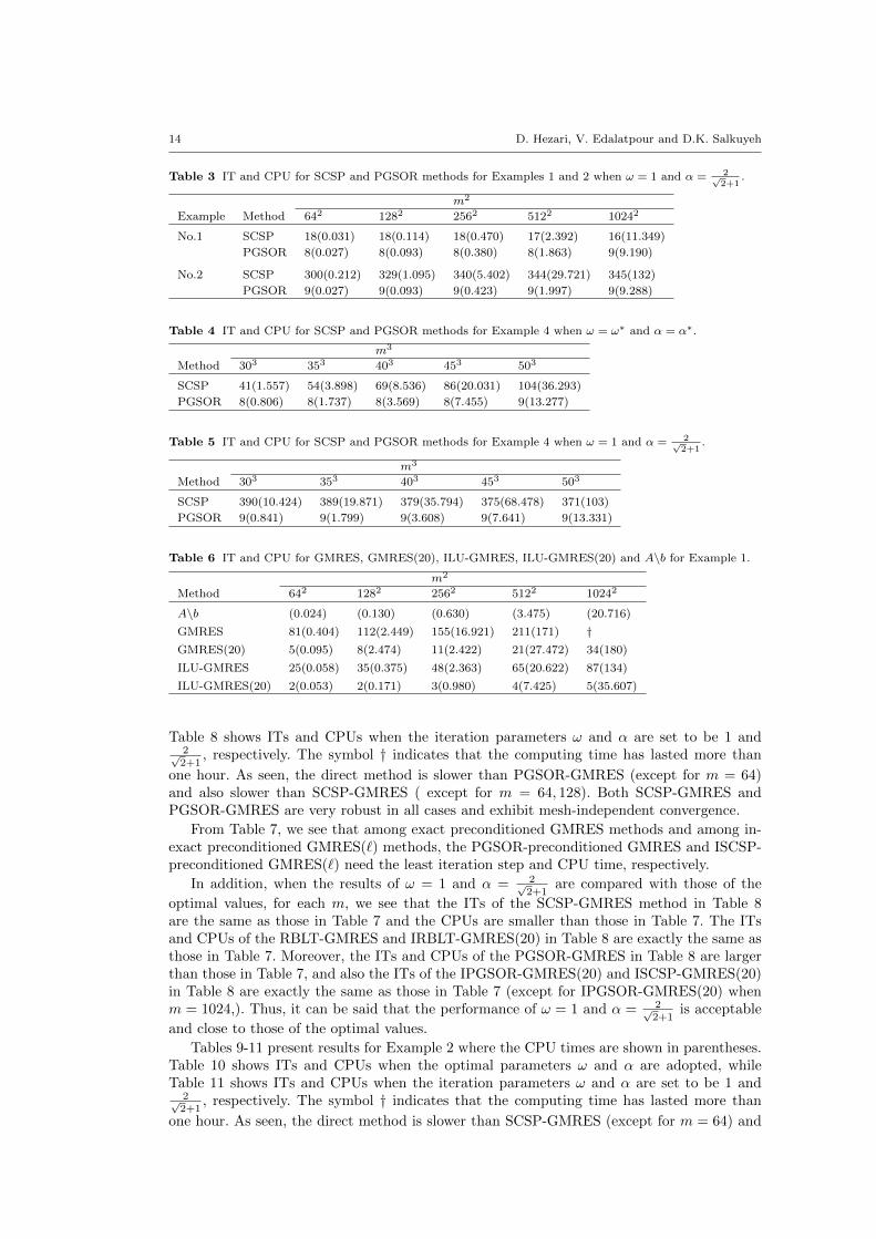
The number of iteration steps and the CPU times for the PGSOR and SCSP methodsfor the examples 1, 2 and 4 with respect to different values of the problem size m, are listedin Tables 2-5, where the CPU times are shown in parentheses. Tables 2 and 4 show ITs andCPUs when the optimal parameters ω and α are adopted, while Tables 3 and 5 show ITs andCPUs when the iteration parameters ω and α are set to be 1 and 2√
2+1, respectively. Note
that the SCSP method is employed for solving the original complex system (1), while PGSORmethod is employed for solving equivalent block two-by-two system (2). At each step of thePGSOR method, it is required to solve two subsystems with the coefficient matrix ωW + T ,while in SCSP method one subsystem with the same coefficient matrix is required. In Table 2we can see that the number of iterations of the SCSP method for Example 1 are almost twiceas much as that of the PGSOR method, but the their computing times are close together. Asseen, the PGSOR iteration method outperforms the SCSP iteration method.
In addition, when the results of ω = 1 and α = 2√2+1
are compared with those of the
optimal values, for each m, we see that the ITs and CPUs of the PGSOR and SCSP methodsin Tables 3 and 5 are larger than those in Tables 2 and 4, respectively. However, for Example1, it can be mentioned that the performance of ω = 1 and α = 2√
2+1is acceptable and close
to those of the optimal values and also, for Examples 2 and 4, the performance of the PGSORmethod with ω = 1 and α = 2√
2+1is acceptable and close to those of the optimal values,
while performance of the SCSP method with ω = 1 is far away those of the optimal values.Tables 6-8 present results for Example 1 where the CPU times are shown in parentheses.
Table 7 shows ITs and CPUs when the optimal parameters ω and α are adopted, while
14 D. Hezari, V. Edalatpour and D.K. Salkuyeh
Table 3 IT and CPU for SCSP and PGSOR methods for Examples 1 and 2 when ω = 1 and α = 2√2+1
.
m2
Example Method 642 1282 2562 5122 10242
No.1 SCSP 18(0.031) 18(0.114) 18(0.470) 17(2.392) 16(11.349)
PGSOR 8(0.027) 8(0.093) 8(0.380) 8(1.863) 9(9.190)
No.2 SCSP 300(0.212) 329(1.095) 340(5.402) 344(29.721) 345(132)
PGSOR 9(0.027) 9(0.093) 9(0.423) 9(1.997) 9(9.288)
Table 4 IT and CPU for SCSP and PGSOR methods for Example 4 when ω = ω∗ and α = α∗.
m3
Method 303 353 403 453 503
SCSP 41(1.557) 54(3.898) 69(8.536) 86(20.031) 104(36.293)
PGSOR 8(0.806) 8(1.737) 8(3.569) 8(7.455) 9(13.277)
Table 5 IT and CPU for SCSP and PGSOR methods for Example 4 when ω = 1 and α = 2√2+1
.
m3
Method 303 353 403 453 503
SCSP 390(10.424) 389(19.871) 379(35.794) 375(68.478) 371(103)
PGSOR 9(0.841) 9(1.799) 9(3.608) 9(7.641) 9(13.331)
Table 6 IT and CPU for GMRES, GMRES(20), ILU-GMRES, ILU-GMRES(20) and A\b for Example 1.
m2
Method 642 1282 2562 5122 10242
A\b (0.024) (0.130) (0.630) (3.475) (20.716)
GMRES 81(0.404) 112(2.449) 155(16.921) 211(171) †GMRES(20) 5(0.095) 8(2.474) 11(2.422) 21(27.472) 34(180)
ILU-GMRES 25(0.058) 35(0.375) 48(2.363) 65(20.622) 87(134)
ILU-GMRES(20) 2(0.053) 2(0.171) 3(0.980) 4(7.425) 5(35.607)
Table 8 shows ITs and CPUs when the iteration parameters ω and α are set to be 1 and2√2+1
, respectively. The symbol † indicates that the computing time has lasted more than
one hour. As seen, the direct method is slower than PGSOR-GMRES (except for m = 64)and also slower than SCSP-GMRES ( except for m = 64, 128). Both SCSP-GMRES andPGSOR-GMRES are very robust in all cases and exhibit mesh-independent convergence.
From Table 7, we see that among exact preconditioned GMRES methods and among in-exact preconditioned GMRES(`) methods, the PGSOR-preconditioned GMRES and ISCSP-preconditioned GMRES(`) need the least iteration step and CPU time, respectively.
In addition, when the results of ω = 1 and α = 2√2+1
are compared with those of the
optimal values, for each m, we see that the ITs of the SCSP-GMRES method in Table 8are the same as those in Table 7 and the CPUs are smaller than those in Table 7. The ITsand CPUs of the RBLT-GMRES and IRBLT-GMRES(20) in Table 8 are exactly the same asthose in Table 7. Moreover, the ITs and CPUs of the PGSOR-GMRES in Table 8 are largerthan those in Table 7, and also the ITs of the IPGSOR-GMRES(20) and ISCSP-GMRES(20)in Table 8 are exactly the same as those in Table 7 (except for IPGSOR-GMRES(20) whenm = 1024,). Thus, it can be said that the performance of ω = 1 and α = 2√
2+1is acceptable
and close to those of the optimal values.
Tables 9-11 present results for Example 2 where the CPU times are shown in parentheses.Table 10 shows ITs and CPUs when the optimal parameters ω and α are adopted, whileTable 11 shows ITs and CPUs when the iteration parameters ω and α are set to be 1 and
2√2+1
, respectively. The symbol † indicates that the computing time has lasted more than
one hour. As seen, the direct method is slower than SCSP-GMRES (except for m = 64) and
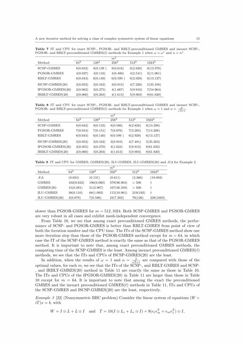
A new iterative method for solving a class of complex symmetric system of linear equations 15
Table 7 IT and CPU for exact SCSP-, PGSOR- and RBLT-preconditioned GMRES and inexact SCSP-,PGSOR- and RBLT-preconditioned GMRES(`) methods for Example 1 when ω = ω∗ and α = α∗.
m2
Method 642 1282 2562 5122 10242
SCSP-GMRES 8(0.042) 8(0.139 ) 8(0.618) 8(2.828) 8(13.378)
PGSOR-GMRES 4(0.037) 4(0.116) 4(0.480) 4(2.541) 5(11.961)
RBLT-GMRES 6(0.043) 6(0.140) 6(0.599 ) 6(2.929) 6(13.127)
ISCSP-GMRES(20) 2(0.052) 2(0.162) 3(0.915) 4(7.226) 5(35.458)
IPGSOR-GMRES(20) 2(0.062) 3(0.275) 4(1.667) 5(9.910) 7(54.964)
IRBLT-GMRES(20) 2(0.060) 3(0.263) 4(1.613) 5(9.903) 8(61.820)
Table 8 IT and CPU for exact SCSP-, PGSOR- and RBLT-preconditioned GMRES and inexact SCSP-,PGSOR- and RBLT-preconditioned GMRES(`) methods for Example 1 when ω = 1 and α = 2√
2+1.
m2
Method 642 1282 2562 5122 10242
SCSP-GMRES 8(0.042) 8(0.133) 8(0.586) 8(2.828) 8(13.298)
PGSOR-GMRES 7(0.044) 7(0.151) 7(0.676) 7(3.265) 7(14.268)
RBLT-GMRES 6(0.043) 6(0.140) 6(0.599 ) 6(2.929) 6(13.127)
ISCSP-GMRES(20) 2(0.052) 2(0.162) 3(0.910) 4(7.481) 5(35.263)
IPGSOR-GMRES(20) 2(0.055) 3(0.270) 4(1.623) 5(9.912) 8(61.032)
IRBLT-GMRES(20) 2(0.060) 3(0.263) 4(1.613) 5(9.903) 8(61.820)
Table 9 IT and CPU for GMRES, GMRES(20), ILU-GMRES, ILU-GMRES(20) and A\b for Example 2.
m2
Method 642 1282 2562 5122 10242
A\b (0.024) (0.131) (0.611) (3.366) (19.893)
GMRES 102(0.622) 196(6.060) 379(96.904) > 500 †GMRES(20) 15(0.281) 51(2.967) 167(36.359) > 500 †ILU-GMRES 38(0.110) 68(1.092) 115(10.961) 219(192) †ILU-GMRES(20) 3(0.078) 7(0.586) 23(7.202) 70(126) 228(1603)
slower than PGSOR-GMRES for m = 512, 1024. Both SCSP-GMRES and PGSOR-GMRESare very robust in all cases and exhibit mesh-independent convergence.
From Table 10, we see that among exact preconditioned GMRES methods, the perfor-mance of SCSP- and PGSOR-GMRES is better than RBLT-GMRES from point of view ofboth the iteration number and the CPU time. The ITs of the SCSP-GMRES method show onemore iteration step than those of the PGSOR-GMRES method except for m = 64, in whichcase the IT of the SCSP-GMRES method is exactly the same as that of the PGSOR-GMRESmethod. It is important to note that, among exact preconditioned GMRES methods, thecomputing time of the SCSP-GMRES is the least. Among inexact preconditioned GMRES(`)methods, we see that the ITs and CPUs of ISCSP-GMRES(20) are the least.
In addition, when the results of ω = 1 and α = 2√2+1
are compared with those of the
optimal values, for each m, we see that the ITs of the SCSP-, and RBLT-GMRES and SCSP-, and IRBLT-GMRES(20) method in Table 11 are exactly the same as those in Table 10.The ITs and CPUs of the IPGSOR-GMRES(20) in Table 11 are larger than those in Table10 except for m = 64. It is important to note that among the exact the preconditionedGMRES and the inexact preconditioned GMRES(`) methods in Table 11, ITs and CPUs ofthe SCSP-GMRES and ISCSP-GMRES(20) are the least, respectively.
Example 3 [22] (Nonsymmetric BBC problem) Consider the linear system of equations (W +iT )x = b, with
W = I ⊗ L+ L⊗ I and T = 10(I ⊗ Lc + Lc ⊗ I) + 9(e1eTm + eme
T1 )⊗ I,

16 D. Hezari, V. Edalatpour and D.K. Salkuyeh
Table 10 IT and CPU for exact SCSP-, PGSOR- and RBLT-preconditioned GMRES and inexact SCSP-,PGSOR- and RBLT-preconditioned GMRES(`) methods for Example 2 when ω = ω∗ and α = α∗.
m2
Method 642 1282 2562 5122 10242
SCSP-GMRES 7(0.040) 7(0.124) 7(0.529) 7(2.637) 7(12.128)
PGSOR-GMRES 7(0.046) 6(0.145) 6(0.681) 6(2.831) 6(13.279)
RBLT-GMRES 8(0.049) 8(0.162) 8(0.730) 8(3.574) 8(15.938)
ISCSP-GMRES(20) 3(0.071) 7(0.525) 23(7.036) 70(125) 228(1579)
IPGSOR-GMRES(20) 9(0.205) 20(1.723) 58(23.424) 190(366) > 500
IRBLT-GMRES(20) 9(0.202) 23(1.943) 73(29.034) 242(505) > 500
Table 11 IT and CPU for exact SCSP-, PGSOR- and RBLT-preconditioned GMRES and inexact SCSP-,PGSOR- and RBLT-preconditioned GMRES(`) methods for Example 2 when ω = 1 and α = 2√
2+1.
m2
Method 642 1282 2562 5122 10242
SCSP-GMRES 7(0.039) 7(0.124) 7(0.523) 7(2.591) 7(12.099)
PGSOR-GMRES 8(0.049) 8(0.163) 8(0.720) 8(3.516) 8(15.876)
RBLT-GMRES 8(0.049) 8(0.162) 8(0.730) 8(3.574) 8(15.938)
ISCSP-GMRES(20) 3(0.071) 7(0.525) 23(7.210) 70(124) 228(1577)
IPGSOR-GMRES(20) 9(0.199) 23(1.943) 70(27.887) 234(454) > 500
IRBLT-GMRES(20) 9(0.202) 23(1.943) 73(29.034) 242(505) > 500
0 2 4 6 80
1
2
3
4
5
6
7
8
9
1 1 1 1 1−0.25
−0.2
−0.15
−0.1
−0.05
0
0.05
0.1
0.15
0.2
0.25
1 1 1 1 10
0.05
0.1
0.15
0.2
0.25
0.3
0.35
0.4
0.45
0.5
Fig. 2 Eigenvalues distribution of the matrix A (left) and the preconditioned matrix, M−1ω A where ω = ω∗
(middle) and M−1ω A where ω = 1 (right) for Example 1 with m = 32.
0 2 4 6 8−10
−8
−6
−4
−2
0
2
4
6
8
10
1 1.005 1.01 1.015 1.02 1.025−0.015
−0.01
−0.005
0
0.005
0.01
0.015
1 1.02 1.04 1.06 1.08 1.1−0.2
−0.15
−0.1
−0.05
0
0.05
0.1
0.15
0.2
Fig. 3 Eigenvalues distribution of the block two-by-two matrix R (left), the preconditioned matrixP−1(ω∗, α∗)R (middle) and the preconditioned matrix P−1(1, 2√
2+1)R (right) for Example 1 with m = 32.

A new iterative method for solving a class of complex symmetric system of linear equations 17
where L = tridiag(−1− θ, 2,−1 + θ) ∈ Rm×m, θ = 12(m+1) , Lc = L− e1eTm − emeT1 ∈ Rm×m
and e1 and em are the first and last unit vectors in Rm, respectively. We take the right-handside vector b to be b = (1 + i)A1, with 1 being the vector of all entries equal to 1.
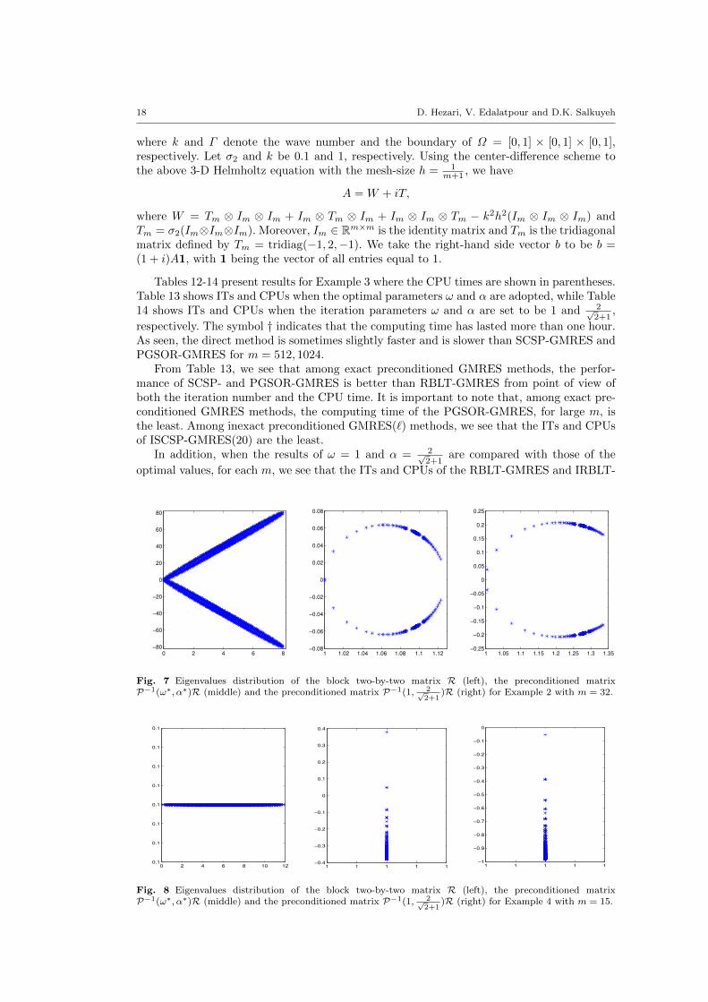
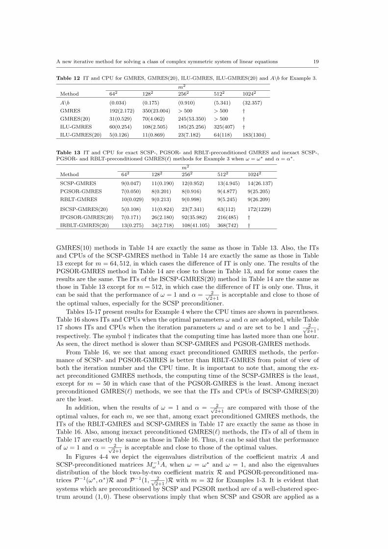
Example 4 [28] Consider the 3-D Helmholtz equation−∆u− k2u+ iσ2u = f(x, y, z), (x, y, z) ∈ Ω = [0, 1]× [0, 1]× [0, 1],u|Γ = g(x, y, z), (x, y, z) ∈ Γ,
0 2 4 6 80.02
0.04
0.06
0.08
0.1
0.12
0.14
0.16
0.18
0.2
1 1 1 1 1−0.8
−0.6
−0.4
−0.2
0
0.2
0.4
0.6
0.8
1 1 1 1 1−1
−0.8
−0.6
−0.4
−0.2
0
0.2
0.4
0.6
Fig. 4 Eigenvalues distribution of the matrix A (left) and the preconditioned matrix, M−1ω A where ω = ω∗
(middle) and M−1ω A where ω = 1 (right) for Example 2 with m = 32.
0 2 4 6 8−0.2
−0.15
−0.1
−0.05
0
0.05
0.1
0.15
0.2
1 1.05 1.1 1.15 1.2
−0.1
−0.05
0
0.05
0.1
1 1.1 1.2 1.3 1.4
−0.2
−0.15
−0.1
−0.05
0
0.05
0.1
0.15
0.2
Fig. 5 Eigenvalues distribution of the block two-by-two matrix R (left), the preconditioned matrixP−1(ω∗, α∗)R (middle) and the preconditioned matrix P−1(1, 2√
2+1)R (right) for Example 2 with m = 32.
0 2 4 6 80
10
20
30
40
50
60
70
80
1 1 1 1 1−0.4
−0.3
−0.2
−0.1
0
0.1
0.2
0.3
0.4
0.5
0.6
1 1 1 1 1−0.1
0
0.1
0.2
0.3
0.4
0.5
0.6
0.7
0.8
0.9
Fig. 6 Eigenvalues distribution of the matrix A (left) and the preconditioned matrix, M−1ω A where ω = ω∗
(middle) and M−1ω A where ω = 1 (right) for Example 3 with m = 32.
18 D. Hezari, V. Edalatpour and D.K. Salkuyeh
where k and Γ denote the wave number and the boundary of Ω = [0, 1] × [0, 1] × [0, 1],respectively. Let σ2 and k be 0.1 and 1, respectively. Using the center-difference scheme tothe above 3-D Helmholtz equation with the mesh-size h = 1
m+1 , we have
A = W + iT,
where W = Tm ⊗ Im ⊗ Im + Im ⊗ Tm ⊗ Im + Im ⊗ Im ⊗ Tm − k2h2(Im ⊗ Im ⊗ Im) andTm = σ2(Im⊗Im⊗Im). Moreover, Im ∈ Rm×m is the identity matrix and Tm is the tridiagonalmatrix defined by Tm = tridiag(−1, 2,−1). We take the right-hand side vector b to be b =(1 + i)A1, with 1 being the vector of all entries equal to 1.
Tables 12-14 present results for Example 3 where the CPU times are shown in parentheses.Table 13 shows ITs and CPUs when the optimal parameters ω and α are adopted, while Table14 shows ITs and CPUs when the iteration parameters ω and α are set to be 1 and 2√
2+1,
respectively. The symbol † indicates that the computing time has lasted more than one hour.As seen, the direct method is sometimes slightly faster and is slower than SCSP-GMRES andPGSOR-GMRES for m = 512, 1024.
From Table 13, we see that among exact preconditioned GMRES methods, the perfor-mance of SCSP- and PGSOR-GMRES is better than RBLT-GMRES from point of view ofboth the iteration number and the CPU time. It is important to note that, among exact pre-conditioned GMRES methods, the computing time of the PGSOR-GMRES, for large m, isthe least. Among inexact preconditioned GMRES(`) methods, we see that the ITs and CPUsof ISCSP-GMRES(20) are the least.
In addition, when the results of ω = 1 and α = 2√2+1
are compared with those of the
optimal values, for each m, we see that the ITs and CPUs of the RBLT-GMRES and IRBLT-
0 2 4 6 8
−80
−60
−40
−20
0
20
40
60
80
1 1.02 1.04 1.06 1.08 1.1 1.12−0.08
−0.06
−0.04
−0.02
0
0.02
0.04
0.06
0.08
1 1.05 1.1 1.15 1.2 1.25 1.3 1.35−0.25
−0.2
−0.15
−0.1
−0.05
0
0.05
0.1
0.15
0.2
0.25
Fig. 7 Eigenvalues distribution of the block two-by-two matrix R (left), the preconditioned matrixP−1(ω∗, α∗)R (middle) and the preconditioned matrix P−1(1, 2√
2+1)R (right) for Example 2 with m = 32.
0 2 4 6 8 10 120.1
0.1
0.1
0.1
0.1
0.1
0.1
0.1
1 1 1 1 1−0.4
−0.3
−0.2
−0.1
0
0.1
0.2
0.3
0.4
1 1 1 1 1−1
−0.9
−0.8
−0.7
−0.6
−0.5
−0.4
−0.3
−0.2
−0.1
0
Fig. 8 Eigenvalues distribution of the block two-by-two matrix R (left), the preconditioned matrixP−1(ω∗, α∗)R (middle) and the preconditioned matrix P−1(1, 2√
2+1)R (right) for Example 4 with m = 15.
A new iterative method for solving a class of complex symmetric system of linear equations 19
Table 12 IT and CPU for GMRES, GMRES(20), ILU-GMRES, ILU-GMRES(20) and A\b for Example 3.
m2
Method 642 1282 2562 5122 10242
A\b (0.034) (0.175) (0.910) (5.341) (32.357)
GMRES 192(2.172) 350(23.004) > 500 > 500 †GMRES(20) 31(0.529) 70(4.062) 245(53.350) > 500 †ILU-GMRES 60(0.254) 108(2.505) 185(25.256) 325(407) †ILU-GMRES(20) 5(0.126) 11(0.869) 23(7.182) 64(118) 183(1304)
Table 13 IT and CPU for exact SCSP-, PGSOR- and RBLT-preconditioned GMRES and inexact SCSP-,PGSOR- and RBLT-preconditioned GMRES(`) methods for Example 3 when ω = ω∗ and α = α∗.
m2
Method 642 1282 2562 5122 10242
SCSP-GMRES 9(0.047) 11(0.190) 12(0.952) 13(4.945) 14(26.137)
PGSOR-GMRES 7(0.050) 8(0.201) 8(0.916) 9(4.877) 9(25.205)
RBLT-GMRES 10(0.029) 9(0.213) 9(0.998) 9(5.245) 9(26.209)
ISCSP-GMRES(20) 5(0.108) 11(0.824) 23(7.341) 63(112) 172(1229)
IPGSOR-GMRES(20) 7(0.171) 26(2.180) 92(35.982) 216(485) †IRBLT-GMRES(20) 13(0.275) 34(2.718) 108(41.105) 368(742) †
GMRES(10) methods in Table 14 are exactly the same as those in Table 13. Also, the ITsand CPUs of the SCSP-GMRES method in Table 14 are exactly the same as those in Table13 except for m = 64, 512, in which cases the difference of IT is only one. The results of thePGSOR-GMRES method in Table 14 are close to those in Table 13, and for some cases theresults are the same. The ITs of the ISCSP-GMRES(20) method in Table 14 are the same asthose in Table 13 except for m = 512, in which case the difference of IT is only one. Thus, itcan be said that the performance of ω = 1 and α = 2√
2+1is acceptable and close to those of
the optimal values, especially for the SCSP preconditioner.
Tables 15-17 present results for Example 4 where the CPU times are shown in parentheses.Table 16 shows ITs and CPUs when the optimal parameters ω and α are adopted, while Table17 shows ITs and CPUs when the iteration parameters ω and α are set to be 1 and 2√
2+1,
respectively. The symbol † indicates that the computing time has lasted more than one hour.As seen, the direct method is slower than SCSP-GMRES and PGSOR-GMRES methods.
From Table 16, we see that among exact preconditioned GMRES methods, the perfor-mance of SCSP- and PGSOR-GMRES is better than RBLT-GMRES from point of view ofboth the iteration number and the CPU time. It is important to note that, among the ex-act preconditioned GMRES methods, the computing time of the SCSP-GMRES is the least,except for m = 50 in which case that of the PGSOR-GMRES is the least. Among inexactpreconditioned GMRES(`) methods, we see that the ITs and CPUs of ISCSP-GMRES(20)are the least.
In addition, when the results of ω = 1 and α = 2√2+1
are compared with those of the
optimal values, for each m, we see that, among exact preconditioned GMRES methods, theITs of the RBLT-GMRES and SCSP-GMRES in Table 17 are exactly the same as those inTable 16. Also, among inexact preconditioned GMRES(`) methods, the ITs of all of them inTable 17 are exactly the same as those in Table 16. Thus, it can be said that the performanceof ω = 1 and α = 2√
2+1is acceptable and close to those of the optimal values.
In Figures 4-4 we depict the eigenvalues distribution of the coefficient matrix A andSCSP-preconditioned matrices M−1ω A, when ω = ω∗ and ω = 1, and also the eigenvaluesdistribution of the block two-by-two coefficient matrix R and PGSOR-preconditioned ma-trices P−1(ω∗, α∗)R and P−1(1, 2√
2+1)R with m = 32 for Examples 1-3. It is evident that
systems which are preconditioned by SCSP and PGSOR method are of a well-clustered spec-trum around (1, 0). These observations imply that when SCSP and GSOR are applied as a
20 D. Hezari, V. Edalatpour and D.K. Salkuyeh
Table 14 IT and CPU for exact SCSP-, PGSOR- and RBLT-preconditioned GMRES and inexact SCSP-,PGSOR- and RBLT-preconditioned GMRES(`) methods for Example 3 when ω = 1 and α = 2√
2+1.
m2
Method 642 1282 2562 5122 10242
SCSP-GMRES 10(0.049) 11(0.190) 12(0.952) 14(5.519) 14(26.209)
PGSOR-GMRES 11(0.050) 10(0.231) 9(0.978) 9(4.832) 9(25.008)
RBLT-GMRES 10(0.029) 9(0.213) 9(0.998) 9(4.945) 9(26.137)
ISCSP-GMRES(20) 5(0.108) 11(0.824) 23(7.341) 64(115) 172(1206)
IPGSOR-GMRES(20) 13(0.275) 33(2.683) 105(40.189) 356(682) †IRBLT-GMRES(20) 13(0.275) 34(2.718) 108(41.105) 368(742) †
Table 15 IT and CPU for GMRES, GMRES(20), ILU-GMRES, ILU-GMRES(20) and A\b for Example 4.
m3
Method 303 353 403 453 503
A\b (2.992) (6.608) (14.676) (185) †GMRES 57(1.121) 64(2.108) 70(3.643) 76(6.195) 81(9.794)
GMRES(20) 5(0.485) 6(0.915) 6(1.350) 6(2.005) 6(2.736)
ILU-GMRES 22(0.301) 24(0.565) 26(0.875) 28(1.492) 29(2.241)
ILU-GMRES(20) 2(0.281) 2(0.448) 2(0.668) 2(0.980) 2(1.599)
Table 16 IT and CPU for exact SCSP-, PGSOR- and RBLT-preconditioned GMRES and inexact SCSP-,PGSOR- and RBLT-preconditioned GMRES(`) methods for Example 4 when ω = ω∗ and α = α∗.
m3
Method 303 353 403 453 503
SCSP-GMRES 9(1.134) 10(2.437) 10(4.691) 11(10.074) 12(16.867)
PGSOR-GMRES 8(1.279) 7(2.456) 8(4.865) 8(10.086) 8(16.510)
RBLT-GMRES 9(1390) 9(2.852) 9(5.238) 9(10.660) 9(17.462)
ISCSP-GMRES(20) 2(0.263) 2(0.417) 2(0.627) 2(0.932) 2(1.329)
IPGSOR-GMRES(20) 3(0.441) 3(0.707) 3(1.063) 3(1.972) 3(2.539)
IRBLT-GMRES(20) 3(0.441) 3(0.709) 3(1.069) 3(1.779) 3(2.542)
Table 17 IT and CPU for exact SCSP-, PGSOR- and RBLT-preconditioned GMRES and inexact SCSP-,PGSOR- and RBLT-preconditioned GMRES(`) methods for Example 4 when ω = 1 and α = 2√
2+1.
m3
Method 303 353 403 453 503
SCSP-GMRES 9(1.170) 10(2.430) 10(4.943) 11(9.851) 12(17.053)
PGSOR-GMRES 9(1.384) 9(2.746) 9(5.199) 9(10.605) 9(17.396)
RBLT-GMRES 9(1390) 9(2.852) 9(5.238) 9(10.660) 9(17.462)
ISCSP-GMRES(20) 2(0.262) 2(0.419) 2(0.630) 2(0.906) 2(1.357)
IPGSOR-GMRES(20) 3(0.445) 3(0.707) 3(1.064) 3(1.825) 3(2.544)
IRBLT-GMRES(20) 3(0.44) 3(0.709) 3(1.069) 3(1.779) 3(2.542)
preconditioner for GMRES, the rate of convergence can be improved considerably. This factis further confirmed by the numerical results presented in Tables 7-14.
5 Conclusion
In this paper we have presented a new stationary iterative method, called Scale-Splitting(SCSP) method, for solving original complex linear system (1). Convergence properties ofthe method have been also investigated. We have further explored algebraic and convergenceproperties of the PGSOR iteration method for solving the block two-by-two equivalent linear
A new iterative method for solving a class of complex symmetric system of linear equations 21
system (2) obtained from (1). We also analyzed the eigenvalue properties of the SCSP andPGSOR preconditioned matrices. Both theoretical analysis and numerical performances haveshown that the SCSP and PGSOR iteration methods, and the SCSP and PGSOR precondi-tioners at accelerating the convergence rates of Krylov subspace iteration methods such asGMRES for solving the linear system (1) and (2), respectively, are competitive, and theyare advantageous over rotated block triangular preconditioners. Moreover, we presented theISCSP and IPGSOR preconditioning matrices to precondition linear system (1) and (2),respectively, based on the SCSP and PGSOR preconditioners and showed the effectivenessof these preconditioners at accelerating the convergence rates of Krylov subspace iterationmethods such as GMRES on the basis of numerical results.
Acknowledgements The authors would like to thank the anonymous referees for their valuable commentsand suggestions which substantially improved the quality of the paper. The work of the second author ispartially supported by University of Guilan.
References
1. R. Hiptmair, Finite elements in computational electromagnetism, Acta Numer. 11 (2002) 237-339.2. U. van Rienen, Numerical methods in computational electrodynamics: linear systems in practical applica-
tions, Springer, Berlin (2001).3. D. Bertaccini, Efficient solvers for sequences of complex symmetric linear systems, Electr. Trans. Numer.
Anal. 18 (2004) 49-64.4. A. Feriani, F. Perotti and V. Simoncini, Iterative system solvers for the frequency analysis of linear me-
chanical systems, Comput. Methods Appl. Mech. Eng. 190 (2000) 1719-1739.5. S. R. Arridge, Optical tomography in medical imaging, Inverse Probl. 15 (1999) 41-93.6. W. V. Dijk and F. M. Toyama, Accurate numerical solutions of the time-dependent Schrodinger equation,
Phys. Rev. E. 75 (2007) 1-10.7. B. Poirier, Efficient preconditioning scheme for block partitioned matrices with structured sparsity, Numer.
Linear Algebra Appl. 7 (2000) 715-726.8. M. Benzi, D. Bertaccini, Block preconditioning of real-valued iterative algorithms for complex linear sys-
tems, IMA J. Numer. Anal. 28 (2008) 598-618.9. Z. Z. Bai, G. H. Golub and M. K. Ng, Hermitian and skew-Hermitian splitting methods for non-Hermitian
positive definite linear systems, SIAM J. Matrix Anal. Appl. 24 (2003) 603-626.10. Z. Z. Bai, M. Benzi and F. Chen, Modified HSS iteration methods for a class of complex symmetric linear
systems, Computing 87 (2010) 93-111.11. Z. Z. Bai, M. Benzi and F. Chen, On preconditioned MHSS iteration methods for complex symmetric
linear systems, Numer. Algor. 56 (2011) 297-317.12. X. Li, A. L. Yang and Y. J. Wu, Lopsided PMHSS iteration method for a class of complex symmetric
linear systems, Numer. Algor. 66 (2014) 555-568.13. H. A. van der Vorst and J. B. M. Melissen, A Petrov-Galerkin type method for solving Ax = b, where A
is symmetric complex, IEEE Trans. Mag. 26 (1990) 706-708.14. R. W. Freund, Conjugate gradient-type methods for linear systems with complex symmetric coefficient
matrices, SIAM J. Sci. Stat. Comput. 13 (1992) 425-448.15. T. Sogabe and S. L. Zhang, A COCR method for solving complex symmetric linear systems, J. Comput.
Appl. Math. 199 (2007) 297-303.16. X. M. Gu, M. Clemens, T. Z. Huang, L. Li, The SCBiCG class of algorithms for complex symmetric linear
systems with applications in several electromagnetic model problems, Comput. Phys. Commun. 191 (2015)52-64.
17. X. M. Gu, T. Z. Huang, L. Li, H.-B. Li, T. Sogabe, M. Clemens, Quasi-minimal residual variants of theCOCG and COCR methods for complex symmetric linear systems in electromagnetic simulations, IEEETrans. Microw. Theory Tech. 62 (2014) 2859-2867.
18. Z. Z. Bai, M. Benzi and F. Chen, Preconditioned MHSS iteration methods for a class of block two-by-twolinear systems with applications to distributed control problems, IMA J. Numer. Anal. 33 (2013) 343-369.
19. D. K. Salkuyeh, D. Hezari and V. Edalatpour, Generalized SOR iterative method for a class of complexsymmetric linear system of equations, Int. J. Comput. Math. 92 (2015) 802–815.
20. Z. Z. Bai, On preconditioned iteration methods for complex linear systems, J. Engrg. Math. 93 (2015)41-60.
21. Z. Z. Bai, F. Chen and Z. Q. Wang, Additive block diagonal preconditioning for block two-by-two linearsystems of skew-Hamiltonian coefficient matrices, Numer. Algor. 64 (2013) 655-675.
22. Z. Z. Bai, Rotated block triangular preconditioning based on PMHSS, Sci. China Math. 56 (2013) 2523-2538.
23. C. Lang, Z.-R. Ren, Inexact rotated block triangular preconditioners for a class of block two-by-twomatrices, J. Engrg. Math. 93 (2015) 87-98.

22 D. Hezari, V. Edalatpour and D.K. Salkuyeh
24. D. Hezari, V. Edalatpour and D. K. Salkuyeh, Preconditioned GSOR iteration method for a class ofcomplex symmetric linear system, Numer. Linear Algebra Appl. 22 (2015) 761–776.
25. Y. Saad and M.H. Schultz, GMRES: A generalized minimal residual algorithm for nonsymmetric linearsystems, SIAM J. Sci. Statist. Comput. 7 (1986) 856-869.
26. Z. Z. Bai, Structured preconditioners for nonsingular matrices of block two-by-two structures, Math.Comput. 75 (2006) 791-815.
27. Z. Z. Bai and M. K. Ng, On inexact preconditioners for nonsymmetric matrices, SIAM J. Sci. Comput.26 (2005) 1710-1724.
28. J. Zhang and H. Dai, A new splitting preconditioner for the iterative solution of complex symmetricindefinite linear systems, Appl. Math. Lett. 49 (2015) 100-106.