Magnetostatic Analysis on ITER Test Blanket Modules

Emiliano D’Alessandro e.dalessandro@enginsoft.it

Andrea Serra

a.serra@enginsoft.it

Giovanni Falcitelli g.falcitelli@enginsoft.it

Agostino Monorchio

a.monorchio@iet.unipi.it

Outline

• What is ITER.

• EnginSoft and University of Pisa activities for ITER.

• Magnetostatic analysis on ITER test Blanket Modules

• EMAG simulation

• Maxwell simulation

• Comparison of results and conclusions

ITER (acronym of International Thermonuclear Experimental Reactor) is an international nuclear fusion research and engineering project, which is building the world’s largest experimental Tokamak nuclear fusion reactor in the south of France. The ‘Tokamak’ concept is based on the magnetic confinement, in which the plasma is contained in a doughnut-shaped vacuum vessel. The fuel, a mixture of deuterium and tritium, two isotopes of hydrogen, is heated to temperatures in excess of 150 million °C, forming a hot plasma.

Cross section of ITER

The fusion between Deuterium and Tritium

What is ITER

ITER construction site Cadarache (Fr)

Main fields of activities concern:

Electromagnetic and electromechanical analysis: Calculation of Lorentz forces and moment due to disruption phenomena Calculation of forces on magnetic experimental objects

Structural analysis: Stress and displacement on ITER assembly due to

seismic loads Welding process simulation.

Eddy current plot on Blanket 1 front wall 10° geometry section of ITER

EnginSoft and Unipi activities for ITER

ITER hangar and seismic displacement

One of the most important issues concerning the plasma behavior is the plasma disruption phenomenon. A disruption is a violent event that terminates a magnetically confined plasma. A magnetic effect of a disruption is the generation of large magnetic forces on the metallic structures surrounding the plasma. This phenomenon is associated to the sudden loss and displacement of the net plasma current that induces eddy current in the metallic structures. According to the Lorentz formula: F = J X B • The activity concerns the time-history calculation of torques and net forces among the Shielding module, FW beam and

the FW fingers of Blanket1 during a plasma disruption.

Electro-mechanical analyses of ITER blanket module number 1

First step of the analysis is the calculation of current density occurring in plasma during disruption phenomena. The disruption phenomena is described by

location and amplitude of current filaments occurring in plasma.

Plasma current density during plasma disruption

Total toroidal current VS Time [ms]

Mesh details

One of the most important issues concerning the plasma behavior is the plasma disruption phenomenon. A disruption is a violent event that terminates a magnetically confined plasma. A magnetic effect of a disruption is the generation of large magnetic forces on the metallic structures surrounding the plasma. This phenomenon is associated to the sudden loss and displacement of the net plasma current that induces eddy current in the metallic structures. According to the Lorentz formula: F = J X B • The activity concerns the time-history calculation of torques and net forces among the Shielding module, FW beam and

the FW fingers of Blanket1 during a plasma disruption.

Electro-mechanical analyses of ITER blanket module number 1

Plasma current densities VS time, output of the first step of the analysis, represent the input data. The second step of the analysis is the calculation of eddy currents on metallic

components of ITER and following assessment of Lorentz forces.

Force calculation: Fy[N] vs time[s] calculated on Blanket1 due to poloidal field variation. Front wall of Blanket module 1. Eddy current

assessment at different time steps

-120000

-100000

-80000

-60000

-40000

-20000

0

20000

40000

1,0600E+01 1,0630E+01 1,0660E+01 1,0690E+01

Fy(N)_ES

Fy(N)_ES

Europe is currently developing two Test Blanket Modules (TBMs): the Helium-Cooled Lithium-Lead (HCLL) concept which uses the Lithium-Lead as both breeder and neutron multiplier, and the Helium-Cooled Pebble-Bed (HCPB) concept which features lithium ceramic pebbles as breeder and beryllium pebbles as neutron multiplier. Both concepts use Reduced Activation Ferritic Martensitic (RAFM) steel as structural material, the EUROFER.

Magnetostatic analysis on ITER test Blanket Modules

The TBMs of both HCLL and HCPB concepts will be inserted in an equatorial Port of ITER and connected to the auxiliary systems through a system of pipes, components, and supporting structures located

inside the Port Cell.

Equatorial port of ITER

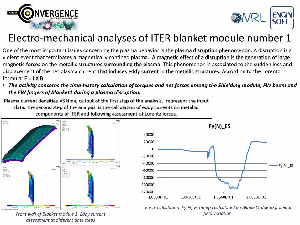
Volumetric geometry of the computational domain (left), of the two incapsulated TBMs (center), and the generated mesh (right).

The two TBMs were modeled as two solid blocks, placed inside each one of the 18 equatorial ports in a symmetric position with respect to the port poloidal midplane.

Use of SOLID96 elements, by implementing the scalar potential method.

Current loads with SOURCE36 elements.

Boundary elements with INFIN111 elements.

Cyclic even symmetry boundary conditions applied via CYCLIC APDL command

EMAG: FEM modeling

Mesh on the TBMs and on the layer surrounding the TBMs

The entire model is made of 977706 elements and 1032234 nodes. The boundary elements, INFIN111 are 16812 with 34992 nodes. All the remaining elements are SOLID96. Each TBM is made of 4800 elements and 5797 nodes. The layer of mesh elements surrounding each TBM is composed of 2112 elements and 4236 nodes. The size and shape

of each element is suitable for an accurate calculation of forces and moments.

A layer of mesh elements surrounding each TBM was generated to accurately calculate forces and moments.

EMAG: FEM modeling

B-H curve data for the TBMs (EUROFER)

H(A/m) B(T)

0 0

1000 0.0893

5000 0.2866

10000 0.5333

20000 1.02667

30000 1.4032

40000 1.6102

50000 1.7128

100000 1.8956

200000 2.0513

300000 2.18255

400000 2.310155

500000 2.436719

1000000 3.066237

H(A/m) B_HCLL (T) B_HCPB (T)

0.00000 0.00000 0.00000

1000.00000 0.03427 0.04039

2000.00000 0.05356 0.06301

3000.00000 0.07284 0.08563

4000.00000 0.09212 0.10825

5000.00000 0.11140 0.13087

6000.00000 0.13069 0.15350

7000.00000 0.14998 0.17612

8000.00000 0.16927 0.19875

9000.00000 0.18855 0.22138

10000.00000 0.20784 0.24400

20000.00000 0.40071 0.47026

30000.00000 0.54976 0.64459

40000.00000 0.63524 0.74357

50000.00000 0.68157 0.79615

100000.00000 0.78939 0.91230

200000.00000 0.92631 1.05131

300000.00000 1.05407 1.17946

400000.00000 1.18046 1.30598

500000.00000 1.30646 1.43204

600000.00000 1.43221 1.55781

700000.00000 1.55796 1.68358

800000.00000 1.68371 1.80935

900000.00000 1.80946 1.93511

1000000.00000 1.93521 2.06088

Equivalent smeared B-H data used for TBMs

It was assumed that in the HCPB the ratio metal/no metal is 0.8, while in the HCLL it is 0.6, therefore equivalent smeared properties were used.

EMAG: Material properties

Formula used to obtain smeared BH curve

The superconducting coil system is made of three kinds of coils:

Poloidal Field (PF),

Toroidal Field (TF),

Center Solenoid (CS).

Excitation currents applied through the SOURCE36 elements.

TF excitation currents

PF excitation currents

CS excitation currents

Plasma excitation current

EMAG: Loads and boundary condition

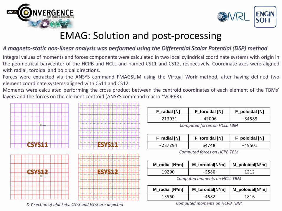
A magneto-static non-linear analysis was performed using the Differential Scalar Potential (DSP) method

Integral values of moments and forces components were calculated in two local cylindrical coordinate systems with origin in the geometrical barycenter of the HCPB and HCLL and named CS11 and CS12, respectively. Coordinate axes were aligned with radial, toroidal and poloidal directions. Forces were extracted via the ANSYS command FMAGSUM using the Virtual Work method, after having defined two element coordinate systems aligned with CS11 and CS12. Moments were calculated performing the cross product between the centroid coordinates of each element of the TBMs’ layers and the forces on the element centroid (ANSYS command macro *VOPER).

EMAG: Solution and post-processing

B field on full assembly . B field on blankets.

CSYS11

CSYS12

ESYS11

ESYS12

F_radial [N] F_toroidal [N] F_poloidal [N]

-213931 -42006 -34589

Computed forces on HCLL TBM

F_radial [N] F_toroidal [N] F_poloidal [N]

-237294 64748 -49501

Computed forces on HCPB TBM

M_radial [N*m] M_toroidal[N*m] M_poloidal[N*m]

19290 -5580 1212

Computed moments on HCLL TBM

M_radial [N*m] M_toroidal[N*m] M_poloidal[N*m]

13560 -4582 1816

Computed moments on HCPB TBM

A magneto-static non-linear analysis was performed using the Differential Scalar Potential (DSP) method

EMAG: Solution and post-processing

Integral values of moments and forces components were calculated in two local cylindrical coordinate systems with origin in the geometrical barycenter of the HCPB and HCLL and named CS11 and CS12, respectively. Coordinate axes were aligned with radial, toroidal and poloidal directions. Forces were extracted via the ANSYS command FMAGSUM using the Virtual Work method, after having defined two element coordinate systems aligned with CS11 and CS12. Moments were calculated performing the cross product between the centroid coordinates of each element of the TBMs’ layers and the forces on the element centroid (ANSYS command macro *VOPER).

X-Y section of blankets: CSYS and ESYS are depicted

Accuracy of results:

Summary of energetic errors resulting from EMAGERR run

EMAG: Solution and post-processing A magneto-static non-linear analysis was performed using the Differential Scalar Potential (DSP) method

Integral values of moments and forces components were calculated in two local cylindrical coordinate systems with origin in the geometrical barycenter of the HCPB and HCLL and named CS11 and CS12, respectively. Coordinate axes were aligned with radial, toroidal and poloidal directions. Forces were extracted via the ANSYS command FMAGSUM using the Virtual Work method, after having defined two element coordinate systems aligned with CS11 and CS12. Moments were calculated performing the cross product between the centroid coordinates of each element of the TBMs’ layers and the forces on the element centroid (ANSYS command macro *VOPER).

Maxwell: geometry modeling

In Maxwell coils are explicitly modeled along with plasma region.

Geometry volumes are modeled overlapping each other . This model technique speed up modeling and help mesh processing

Geometry model in Maxwell. 20° section is used. In figure (A) the simplified blanket modules used for the analysis are depicted.

A

Maxwell: FEM model In Maxwell the auto-adaptive mesher is used. Adaptive meshing technique start with initial mesh and refines it until required accuracy is met or maximum number of passes is reached. Furthermore convergence on forces values is even requested.

Convergence criteria: Maximum number of passes = 20 Percent error = 1% Percent error on forces = 1.5% Refinement per pass = 30%

Convergence process: total number of passes

Energy error vs passes Number of elements vs passes

Radial components of forces [kN]

vs passes

Maxwell: FEM model In Maxwell the auto-adaptive mesher is used. Adaptive meshing technique start with initial mesh and refines it until required accuracy is met or maximum number of passes is reached. Furthermore convergence on forces values is even requested.

Mesh details of the model: full assembly (A),(B) and simplified blankets (C)

A B C

Maxwell: FEM model In order to verify the correctness of the auto adaptive algorithm, a finer mesh is requested on blanket modules. A body sizing of 0.08 m is imposed.

Finer mesh on coarse mesh are

compared

Radial force on HCLL blanket module: comparison between coarse (red line) and fine (green line) mesh. The two

meshes give the same results Comparison between convergence passes of the two

meshes. Highlighted the number of elements

Solution time: 120min.

Solution time: 26min.

Maxwell: Boundary conditions and excitations In Maxwell boundary and excitations are applied using geometry entities. Master and slave boundary is used to apply cyclic symmetry. This boundary condition matches the magnetic field at the slave boundary to the field at the master boundary based on U and V vectors defined. Current can be assigned to the conductor faces that lie on boundary of simulation domain or sheets that lie completely inside the conductor.

Boundary conditions and excitation : cyclic even symmetry (A), TF coils (B), PF, CS coils and plasma current (C)

A B C A

Maxwell: results

B module on full assembly and blankets is depicted.

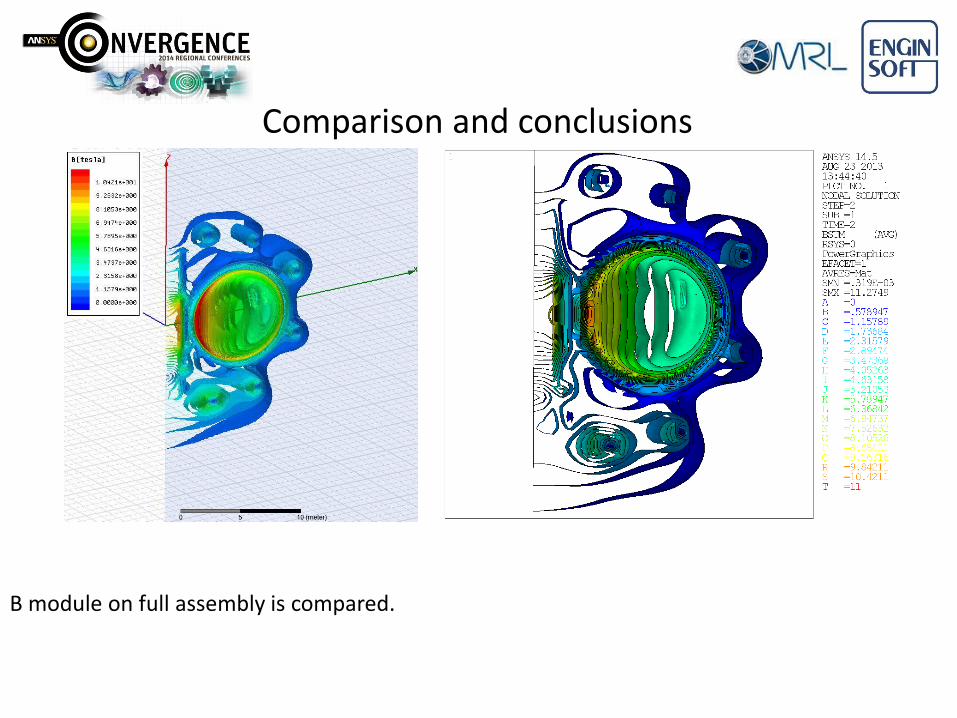
Comparison and conclusions

B module on full assembly is compared.

Comparison and conclusions

B module on simplified blankets modules is compared.

Comparison and conclusions

F_radial [N] F_toroidal [N] F_poloidal [N] Module [N]

-199790 -24233 -28531 203266.57

Computed forces on HCLL TBM

F_radial [N] F_toroidal [N] F_poloidal [N] Module [N

-220980 38846 -44898 228816

Computed forces on HCPB TBM

M_radial

[N*m]

M_toroidal[N*

m]

M_poloidal[N*

m] Module [N*m]

19840 -4530 1239.9 20388

Computed moments on HCLL TBM

M_radial

[N*m]

M_toroidal[N*

m]

M_poloidal[N*

m] Module [N*m]

13953 -3009 1337 14336

Computed moments on HCPB TBM

F_radial [N] F_toroidal [N] F_poloidal [N] Module [N]

-213931 -42006 -34589 220742

Computed forces on HCLL TBM

F_radial [N] F_toroidal [N] F_poloidal [N] Module [N]

-237294 64748 -49501 250900

Computed forces on HCPB TBM

M_radial

[N*m]

M_toroidal[N*

m]

M_poloidal[N*

m] Module [N*m]

19290 -5580 1212 20117

Computed moments on HCLL TBM

M_radial

[N*m]

M_toroidal[N*

m]

M_poloidal[N*

m] Module[N*m]

13560 -4582 1816 14428

Computed moments on HCPB TBM

EMAG forces Maxwell forces

The percentage variation between Maxwell and EMAG forces is about 7.9% on modules. The percentage variation between Maxwell and EMAG moments is about 1.5% on modules. Considering the problem is not confined and the magnetic steel is in saturation, the two software show a good agreement with regard to both field plots and force values

Forces are extracted in Maxwell using the Virtual Work method. In Maxwell moments calculation is straightforward.