Embed Size (px)
Citation preview

ISTANBUL TECHNICAL UNIVERSITY ���� GRADUATE SCHOOL OF SCIENCE ENGINEERING AND TECHNOLOGY
COMPUTATIONAL FLUID DYNAMICS ANALYSIS USING A HIGH-ORDER COMPACT SCHEME ON A GPU
Ph.D. THESIS
Bülent TUTKUN
Department of Aeronautics and Astronautics Engineering
Aeronautics and Astronautics Engineering Graduate Programme
NOVEMBER 2012


ISTANBUL TECHNICAL UNIVERSITY ���� GRADUATE SCHOOL OF SCIENCE ENGINEERING AND TECHNOLOGY
COMPUTATIONAL FLUID DYNAMICS ANALYSIS USING A HIGH-ORDER COMPACT SCHEME ON A GPU
Ph.D. THESIS
Bülent TUTKUN (511032001)
Department of Aeronautics and Astronautics Engineering
Aeronautics and Astronautics Engineering Graduate Programme
Thesis Advisor: Prof. Dr. Fırat Oğuz EDİS
NOVEMBER 2012


İSTANBUL TEKN İK ÜNİVERSİTESİ ���� FEN BİLİMLER İ ENSTİTÜSÜ
GPU ÜZERİNDE YÜKSEK-MERTEBE KOMPAKT ŞEMA KULLANILARAK HESAPLAMALI AKI ŞKANLAR D İNAM İĞİ ANAL İZİ
DOKTORA TEZ İ
Bülent TUTKUN (511032001)
Uçak ve Uzay Mühendisliği Anabilim Dalı
Uçak ve Uzay Mühendisliği Programı
Tez Danışmanı: Prof. Dr. Fırat Oğuz EDİS
KASIM 2012


v
Bulent Tutkun , a Ph.D. student of ITU Graduate School of Science, Engineering and Technology student ID 511032001, successfully defended the dissertation entitled “COMPUTATIONAL FLUID DYNAMICS ANALYSIS US ING A HIGH-ORDER COMPACT SCHEME ON A GPU ”, which he prepared after fulfilling the requirements specified in the associated legislations, before the jury whose signatures are below.
Thesis Advisor : Prof. Dr. Fırat Oğuz EDİS .............................. İstanbul Technical University

vi

vii
FOREWORD
First and foremost I would like to offer my sincerest gratitude to my thesis supervisor Prof. Fırat Oğuz Edis who has supported me throughout this study with his invaluable guidance and experience. In addition, I thank all jury members for their directive contributions. I would like to express my great appreciations for Evren Öner for his help whenever I need it. Without him, it would be very formidable for me to tackle some hardware and software issues. I am also grateful to Asst. Prof. Bayram Çelik for his constructive comments on some parts of this dissertation. I wish to thank to my dearest family members starting from my parents Osman and Nazmiye Tutkun; my elder sister Tülay Tutkun for their heartfelt, continuous support. Finally, a special thanks goes to my beloved wife Gülcan for her patience, enthusiasm and love throughout this study. Also, I should mention that required financial support to get the computer system needed for this study is provided by the Istanbul Technical University support programme for postgraduate researches.
April 2012 Bülent TUTKUN

viii

ix
TABLE OF CONTENTS
Page
FOREWORD ............................................................................................................ vii ABBREVIATIONS ................................................................................................... xi LIST OF TABLES .................................................................................................. xiii LIST OF FIGURES ................................................................................................. xv SUMMARY ............................................................................................................ xvii ÖZET ........................................................................................................................ xix 1. INTRODUCTION .............................................................................................. 1
2. GOVERNING EQUATIONS ............................................................................ 7
2.1 2D Advection Equations and 3D Compressible Navier-Stokes Equations ... 7
2.2 3D Incompressible Navier-Stokes Equations ................................................ 9
3. NUMERICAL METHODS .............................................................................. 11
3.1 Temporal Discritization: Runge-Kutta and Adams-Bashforth Method ...... 11 3.2 High-Order Central Compact Finite Difference Scheme ............................ 12
3.3 High-Order Low-Pass Filtering Scheme ..................................................... 23
3.4 Immersed Boundary Method ....................................................................... 26
3.4.1 Continuous Forcing Approach ............................................................. 26
3.4.2 Direct Forcing Approach...................................................................... 28
3.5 Conjugate Gradient Method ........................................................................ 31
4. GENERAL-PURPOSE GPU (GPGPU) COMPUTING ............................... 37 4.1 GPU Computing in CFD ............................................................................. 38
5. GPU ARCHITECTURE AND CODE DESIGN ............................................ 41 5.1 Tesla C1060 and CUDA .............................................................................. 41
5.2 Code Design ................................................................................................ 43 6. APPLICATIONS AND PERFORMANCE COMPARISONS ..................... 49
6.1 Advection of a Vortical Disturbance ........................................................... 50
6.2 Temporal Mixing Layer .............................................................................. 53
6.3 IBM Test Case - Flow Around a Square Cylinder ...................................... 58
7. CONCLUSIONS ............................................................................................... 75 7.1 Future Works ............................................................................................... 77
REFERENCES ......................................................................................................... 79 APPENDICES .......................................................................................................... 87
APPENDIX A: Fourier Error Analysis of Some Central Finite Difference Schemes for First and Second Derivatives ............................................................................ 87
CURRICULUM VITAE .......................................................................................... 91

x

xi
ABBREVIATIONS
BLAS : Basic Linear Algebra Subroutines CFD : Computational Fluid Dynamics CG : Conjugate Gradient COO : Coordinate Format CPU : Central Processing Unit CSR : Compressed Sparse Row Format CUBLAS : Basic Linear Algebra Subroutines for CUDA CUDA : Compute Unified Device Architecture CUSPARSE : Sparse Matrix Library for CUDA DNS : Direct Numerical Simulation FFT : Fast Fourier Transform GFLOPS : Giga Floating-Point Operations per Second GPGPU : General-Purpose Computing on Graphical Processing Units GPU : Graphical Processing Unit IBM : Immersed Boundary Method IFORT : Intel Fortran Compiler LAPACK : Linear Algebra Package LES : Large Eddy Simulation RHS : Right Hand Side SpMV : Sparse Matrix-Vector Multiplication

xii

xiii
LIST OF TABLES
Page
Table 3.1: Coefficients of Runge-Kutta scheme. ...................................................... 11
Table 3.2: Relations between the coefficients for the first derivative. ...................... 13
Table 3.3: Relations between the coefficients for the second derivative. ................. 15
Table 3.4: Resolution indications of various schemes. ............................................. 19
Table 3.5: Filtering coefficients for various schemes. .............................................. 24
Table 5.1: General specifications of Tesla C1060 [84] ............................................. 41
Table 5.2: Performance gain obtained from the improvements in memory access. . 47
Table 6.1: Absolute errors for the GPU calculations. ............................................... 51
Table 6.2: Required Gflop per time step. .................................................................. 55
Table 6.3: Dimensions of the flow domain. .............................................................. 59
Table 6.4: First node distance from the body. ........................................................... 60
Table 6.5: Comparison of Strouhal numbers for �� = 100. .................................... 67
Table 6.6: Comparison for the variation of Strouhal number with Re ...................... 67
Table 6.7: Comparison of Clrms and Cdave ................................................................. 69

xiv

xv
LIST OF FIGURES
Page
Figure 3.1 : Resolution characteristics of central schemes for first derivative. ...... 18 Figure 3.2 : Resolution characteristics of central schemes for second derivative. . 21
Figure 3.3 : Dissipation characteristics for different filters (�� = �. ). ............... 25 Figure 3.4 : Dissipation characteristics of tenth-order filtering. ............................. 25
Figure 3.5 : An arbitrary body immersed in a Cartesian mesh. .............................. 26
Figure 3.6 : Vicinity of the immersed boundary. .................................................... 31
Figure 3.7 : Conjugate gradient method algorithm. ................................................ 32
Figure 3.8 : COO format for any sparse matrix A. ................................................. 33
Figure 3.9 : CSR format for any sparse matrix A. .................................................. 33
Figure 3.10 : Format of ELL for a general sparse matrix A. .................................... 34
Figure 5.1 : A Tesla C1060 GPU ............................................................................ 41
Figure 5.2 : General structure of Tesla C1060 ........................................................ 42
Figure 5.3 : A representation of CUDA structure ................................................... 43
Figure 5.4 : Representation of the CUDA grid. ...................................................... 44
Figure 5.5 : Computation structure for a 3D flow domain...................................... 44
Figure 5.6 : Ideal coalesced access pattern. ............................................................ 46
Figure 5.7 : Non-coalesced access pattern of the code. .......................................... 46
Figure 6.1 : Flow domain. ....................................................................................... 50
Figure 6.2 : Comparison of computed vorticity magnitude with exact solution. ... 51 Figure 6.3 : Performance comparison, calculation time for one time step. ............ 52
Figure 6.4 : Performance comparison, speed up values. ......................................... 52
Figure 6.5 : Performance comparison, time taken per node. .................................. 53
Figure 6.6 : Mixing layer flow domain. .................................................................. 54
Figure 6.7 : Evolution of eddies. ............................................................................. 55
Figure 6.8 : Performance comparison, calculation time for one time step. ............ 56
Figure 6.9 : Performance comparison, speed up values. ......................................... 56
Figure 6.10 : Performance comparison, time taken per node. .................................. 57
Figure 6.11 : Timing breakdown of one time step for 1283 mesh on GPU. .............. 57
Figure 6.12 : Immersed boundary flow domain and boundary conditions. .............. 59 Figure 6.13 : a) Instantaneous streamlines, b) � velocity contours .......................... 61
Figure 6.14 : Instantaneous streamlines in the vicinity of square cylinder for a full aavortex shedding cycle, Re = 100 (above: Present study, below: aSharma aand Eswaran [99]). ............................................................... 62
Figure 6.15 : U velocity and pressure contours for a full vortex shedding cycle ..... 64
Figure 6.16 : Comparison of Lr. (Yoon et al. [104], Sharma and Eswaran [99], aRobichaux et al. [98]) .......................................................................... 65
Figure 6.17 : Power spectrum of Cl (left) and Cd (right) for Re = 100. .................... 66
Figure 6.18 : Variation of Strouhal number with Reynolds number. Mentioned astudies: Sen et al. [102], Singh et al. [101], Sharma and Eswaran [99], aSaha et al. [97], Sohankar et al. [105], Robichaux et al. [98], Sohankar aet al. [96], Franke et al. [106], Davis et al. [107]. ............................... 68

xvi
Figure 6.19 : RMS of lift coefficients for the various Reynolds numbers. ............... 69
Figure 6.20 : Time averaged drag coefficients for the various Reynolds numbers. . 70
Figure 6.21 : Timing breakdown of one time step. ................................................... 70
Figure 6.22 : Timing breakdown of CG iterative solver. .......................................... 71
Figure 6.23 : SpMV performance of CUSPARSE library. ....................................... 72
Figure 6.24 : Performance comparison of CUSPARSE and ELLPACK. ................. 73 Figure 6.25 : Time comparison for the solution of sparse linear systems. ................ 74
Figure 6.26 : Timing breakdown of incompressible solver and CG iterative solver aafter the use of ELLPACK form. ........................................................ 74

xvii
COMPUTATIONAL FLUID DYNAMICS ANALYSIS USING A HIGH-ORDER COMPACT SCHEME ON A GPU
SUMMARY
Computational fluid dynamics (CFD) has made a great progress in the past several decades in attaining the satisfactory simulation results of practical and engineering flow problems. Although, the practical problems involving complex structures or high Reynolds number turbulence still constitute a major challenge, applications of direct numerical simulation (DNS) and large eddy simulation (LES) to various formidable turbulent flowfields present some promising results. However, DNS or LES calculations are obliged to tackle high memory requirements and heavy computational burdens, as a result of this, users prefer generally less accurate turbulence models to DNS or LES. But most of the practical fluid mechanics problems involve a broad spectrum of length and time scale. Therefore, hardware, software and numerical methods should be thought in combination in order to obtain the solutions of these flows with acceptable accuracy and performance. The main purpose of this study is actually to form such a combination for CFD applications. That is, numerical methods capable of representing all or most of the relevant scales are needed for the simulation of these flows. The length scales resolved by a computation are determined by the spatial resolution; moreover, the accuracy in the representation of these scales depends on the numerical scheme. One way to tackle this problem is the use of a high-order method. Therefore, in this study, a sixth-order compact finite difference scheme is exploited for the space discretization in order to obtain the flow field simulations of three test cases. These test cases are the advection of a vortical disturbance (2D advection equations), temporal mixing layer (3D compressible flow equations) and flow around a square cylinder (3D incompressible flow equations). All computations are performed on a GPU produced for the scientific computing purposes. Used GPU is NVIDIA Tesla C1060 that has 30 streaming multi-processors, each containing 8 scalar processors, clocked at 1.3 GHz. It also has a 4 GB GDDR3 global memory at 102 GB/s. In addition to sixth-order compact scheme, a tenth-order low pass filtering scheme is also applied to the solution vector to supress the spurious oscillations for 2D advection equations and 3D compressible equations. Moreover for the time integration, a fourth-order Runge-Kutta scheme is exploited for the advection and compressible test cases, whereas incompressible test case benefits from a second-order Adams-Bashforth scheme for time advancement. Another important numerical method applied in the present study is immersed boundary method used in the test case involving flow around a square cylinder. In the most basic terms, this method allows to perform the computations on a uniform Cartesian mesh by inserting a forcing term into the momentum equation to mimic the solid body. Performance of the GPU computations in terms of the calculation time for sample problems are compared with the computation performance of a CPU. Used CPU for the comparisons is AMD Phenom 2.5 GHz.

xviii
The codes running on the GPU are written with a C-based programming language. For this, Compute Unified Device Architecture (CUDA) toolkit which is a complete software development solution for programming CUDA-enabled GPUs is utilized as the code design medium. In the CPU side, code is written with Fortran programming language.
Sixth-order compact scheme and tenth-order filtering scheme generate tridiagonal in general or cyclic tridiagonal if the boundary conditions are periodic. For the solution of these linear systems LAPACK/BLAS library is utilized for the CPU code, while the GPU code exploits the inverse of the coefficient matrices for the solution of the same linear systems by utilizing the CUBLAS library. CUDA thread structure is arranged in a way that each node in the computational mesh is represented by one thread. Moreover, thread blocks are aligned with the x Cartesian axis, so every thread representing the nodes on the same horizontal mesh line takes place on the same thread block.
Coalesced access to the global memory is an important factor affecting the performance of the computation on GPU. If there are uncoalesced reads or writes in the computation process, it may severely degrade the computation performance. In the present study, coalescing appeared as an issue in some parts of the code especially in the kernels related to x-derivative calculations. Shared memory property of the GPU is utilized in order to alleviate this degradation in the performance. Shared memory which is an on-chip memory and much faster than the global memory is accessible for all the threads in the same thread block. As a result, a performance increase is attained by using the shared memory when required.
In conclusion, with these mentioned implementations, above test cases are solved on a GPU and obtained results are compared with those of a CPU in terms of calculation times. For the 2D advection equations some speedup values up to 10x are achieved for different mesh sizes in comparison to CPU computations. Test case involving the 3D compressible equations requires more computational efforts in comparison with the advection test case and achieved speedup values between 14.5x – 16.5x again for various mesh sizes. In the case of incompressible test problem, a Poisson equation must be solved as a difference from the previous two cases, and it takes nearly 90% of calculation time. Therefore, related to this, a comparison is made for the solution of sparse linear systems between present application and another GPU and CPU implementations in the literature. Therefore, it is seen that GPU perfromance in this study achieves speedup values about 3x and 24x considering other GPU and CPU performances respectively.

xix
GPU ÜZERİNDE YÜKSEK-MERTEBE KOMPAKT ŞEMA KULLANILARAK HESAPLAMALI AKI ŞKANLAR D İNAM İĞİ ANAL İZİ
ÖZET
Hesaplamalı akışkanlar dinamiği, gündelik ve mühendislik akış problemlerinin tatmin edici simülasyonlarına ulaşma konusunda son çeyrek asır içerisinde büyük ilerlemeler kaydetmiştir. Karmaşık yapılar içeren veya yüksek Reynolds sayılı akışlar hala büyük zorluklar çıkarsa da, direkt sayısal benzetim (DNS) ve büyük eddy benzetiminin (LES) çeşitli zorluklar içeren türbülanslı akış alanlarına uygulanması bazı umut verici sonuçlar sunmaktadır. Bununla birlikte, türbülanslı akış analizlerinde DNS ve LES yöntemlerini kullanan araştırmacılar özellikle üç-boyutlu akış alanlarının benzetiminde yüksek bellek gereksinimleri ve ağır hesaplama yükleriyle uğraşmak zorunda kalmaktadır. Bunun sonucu olarak, araştırmacılar genel olarak daha az doğruluk taşıyan modelleri DNS ve LES’e tercih etmektedirler. Bununla beraber, karşılaşılan çoğu pratik mühendislik problemine uzunluk ve zaman ölçekleri açısından bakıldığında, pek çok problemin uzunluk ve zamanın geniş bir spektrumunu içerdiği görülür. Bundan dolayı, bu özelliklere sahip türbülanslı akışların çözümünün kabul edilebilir bir doğrulukla yapılabilmesi için kullanılacak sayısal yöntemin yanısıra, donanım ve yazılım özellikleri de önem kazanmaktadır. Bunun için donanım, yazılım ve sayısal yöntemlerin bir arada düşünülmesi gerekir. Kısacası bu akışların daha yüksek doğrulukla benzetimi için ilgili ölçeklerin tümünü veya çoğunu temsil edebilme kabiliyetine sahip sayısal yöntemler, bu sayısal yöntemlerin kabul edilebilir bir hızla çözülebilmesi için uygun donanımsal bileşenler ve son olarak da bu donanımsal bileşenlere uygun olarak oluşturulmuş yazılımlar gerekmektedir. Bu çalışmanın başlıca amacı, böyle bir kombinasyonu hesaplamalı akışkanlar dinamiği uygulamaları için bir araya getirmektir. Bir hesaplamada temsil edilebilecek uzunluk ölçekleri uzaysal çözünürlük tarafından belirlenir. Ayrıca, bu ölçeklerin temsilindeki doğruluk da kullanılan sayısal şemaya bağlıdır. Bu bağlamda gereken yüksek doğruluğu sağlamanın bir yolu da yüksek mertebeden yöntemlerin kullanılmasıdır. Yüksek mertebeden doğruluk içeren yöntemlerin kullanılması hem oluşturulacak sayısal ağın toplam eleman sayısında azalmaya sebep olacak hem de ulaşılacak sonuçların doğruluğunu yükseltecektir. Bu nedenle, bu çalışmada, üç test probleminin akış alanı benzetimlerini elde etmek amacıyla, uzaysal ayrıklaştırma için bir kompakt sonlu fark şeması kullanılmıştır. Bu problemler, bir girdapsal bozuntunun taşınımı (iki boyutlu taşınım denklemleri), zamansal karışma tabakası (üç boyutlu sıkıştırılabilir akış denklemleri) ve kare silindir etrafında akıştır (üç boyutlu sıkıştırılamaz akış denklemleri). Yüksek mertebeden kompakt şemalar sahip oldukları özellikler sayesinde hesaplamalı akışkanlar dinamiği alanında oldukça popüler hale gelmişdir. Kompakt sonlu fark şemaları uzunluk ölçeği olarak geniş bir spektruma sahip problemlerde standart sonlu fark şemalarına kıyasla daha iyi bir çözümleme sağlarlar. Ayrıca, kompakt şemalar daha küçük şema açıklıkları gerektirmekte ve özellikle yüksek dalga numaralarında daha iyi bir resolüsyon sağlamaktadır. Bu sayede, kompakt şemalar sonlu fark şemalarının iyi özellikleri ile spektral çözüme benzer bir doğruluğu etkili bir biçimde birleştirirler. Bu özellikler

xx
dikkate alınarak, bu çalışmada akış alanlarının analizinde uzaysal ayrıklaştırma için altıncı-merteben kompakt merkezi sonlu fark şeması kullanılmıştır. Bununla birlikte, merkezi şemalar doğal yapılarında herhangi bir disipasyon taşımadıklarından, sıkıştırılabilir Navier-Stokes denklemlerindeki taşınım terimleri gibi non-linear terimlerin benzetiminde muhtemel non-linear kararsızlıklar ortaya çıkabilir. Bundan dolayı, ortaya çıkabilecek bu türden kararsızlıkları bastırabilmek için kompakt şema ile beraber sıkıştırılabilir akış analizlerinde yüksek-mertebeden alçak geçiren bir filtreleme şeması da kullanılmıştır. Bu yaklaşım, orjinal denklemlerin değiştirilmesini gerektiren yapay disipasyon ekleme yönteminden farklı olarak, bir işlem sonrası yöntemi olarak görülebilir. Bu yaklaşımda filtreleme herbir zaman adımından sonra ulaşılan çözüm vektörüne uygulanmaktadır. Diğer bir deyişle, bu çalışmada kullanılan onuncu-mertebe filtreleme şeması korunumlu değişkenler üzerine koordinat yönleri boyunca art arda uygulanmaktadır.
Bu tez kapsamında kullanılan bir diğer sayısal yöntem ise sıkıştırılamaz akış denklemlerinin çözüldüğü test probleminde kullanılan gömülü sınır yöntemidir. Bu yöntem sınırlardan bağımsız olarak herhangi bir akış alanı için Kartezyen Navier-Stokes çözücülerin kullanılabilmesini sağlayan sayısal bir araçtır. En temel haliyle, bu yaklaşım, momentum denklemine katı cismi taklit etmek amacıyla eklenen bir kuvvet terimi aracılığıyla çözümü üniform kartezyen bir mesh üzerinde yapmamıza olanak tanır. Bu yöntemde oluşturulan sayısal çözüm ağının sınırlara uydurulmasına gerek yoktur. Kartezyen bir grid istenildiği gibi oluşturulur ve sınırlar bu ağın içerisine gömülmüş olarak kabul edilir. İstenilen sınır koşulları, gömülü sınır civarında yönetici denklemlere yapılan müdahaleler yardımıyla sağlanır. Bu sayede karmaşık sınırlar etrafında sayısal çözüm ağı oluşturulması sırasında karşılaşılan zorlukların pek çoğu ortadan kalkar. Bu çalışmada, istenilen sınır koşullarını sağlamak için, gömülü sınırlar civarında momentum denklemlerine gerekli kuvvet terimleri eklenmiş ve sınır koşulları sağlanmıştır.
Ayrıca zaman integrasyonu için, yine ilk iki problem kapsamında dördüncü-mertebeden bir Runge-Kutta şeması uygulanırken, sıkıştırılamaz akış içeren problem için zamansal ilerleme ikinci-mertebeden Adams-Bashforth şeması ile sağlanmıştır.
Daha önce de belirtildiği gibi büyük ölçekli, geniş spektrumlar içeren hesaplamalı akışkanlar dinamiği problemlerinin başarılı bir şekilde çözülmesi sadece kullanılacak uygun sayısal yöntemlere değil aynı zamanda bilgisayar sistemlerinin hesaplama gücündeki gelişmelere de bağlıdır. Bu açıdan bakılınca grafik işleme birimlerinin (GPU) aynı zamanda bilimsel hesaplama birimleri olarak da kullanılmaya başlanması bilgisayar sistemleri açısından önemli bir gelişmedir. GPU’ların hesaplama güçlerindeki sürekli artış, son yıllarda bu birimleri genel olarak hesaplamalı bilimler için ciddi bir alternatif haline sokmuştur. GPU’lar yapıları gereği hızlı paralel görüntü işleme yeteneğine sahip olduklarından, barındırdıkları yüzlerce hesaplama çekirdeği yardımıyla ağır hesaplama yükü içeren mühendislik problemlerinde de başarılı sonuçlar elde etmektedirler. Bu çalışmada, tüm hesaplamalar, bilimsel hesaplamalar için üretilmiş bir GPU üzerinde gerçekleştirilmi ştir. Kullanılan GPU, her biri 8 skalar işlemci içeren 30 adet çoklu-işlemciye sahip olan NVIDIA Tesla C1060 GPU’sudur. Taşıdığı işlemcilerin çalışma frekansları 1.3 GHz olup, 102 GB/sn perfromansında veri iletebilen 4 GB’lık GDDR3 global hafızaya sahiptir. GPU hesaplamalarının performansı örnek problemler için çalışma zamanı açısından bir CPU’nun performansı ile karşılaştırılmıştır. Karşılaştırma için kullanılan CPU AMD Phenom 2.5 GHz’lik CPU’dur.

xxi
Geniş ölçekli problemlerin başarılı bir şekilde çözülmesindeki son faktör oluşturulacak yazılımlardır. Bu çalışmada, problemlerin GPU üzerinde etkili bir şekilde çözülebilmesi için bu donanımsal yapıya ve kullanılan sayısal yöntemlere uygun kodlar geliştirilmi ştir. GPU üzerinde koşan kodlar C-tabanlı bir programlama dili ile yazılmıştır. Bunun için, GPU’ların programlanması için geliştirilen bir ortam olan CUDA (Compute Unified Device Architecture) kullanılmıştır. GPU sonuçlarının karşılaştırıldığı CPU’daki kodlar ise Fortran programlama dili ile yazılmıştır.
Altıncı-mertebe kompakt şema ve onuncu-mertebe filtreleme şeması genel olarak üç-bant katsayı matrisleri üretirler, eğer sınır koşulları periyodik ise katsayı matrisleri periyodik üç-bant olmaktadır. Bu lineer sistemlerin çözümü için CPU kodu LAPACK/BLAS kütüphanesini kullanırken, GPU kodu aynı lineer sistemlerin çözümü için CUBLAS kütüphanesi aracılığı ile katsayı matrislerinin tersini kullanmaktadır. CUDA thread yapısı hesaplama ağındaki herbir düğümün bir thread tarafından temsil edilceği şekilde düzenlenmiştir. Ayrıca thread blokları x Kartezyen ekseni boyunca yer almaktadır, böylece aynı yatay mesh hattı üzerindeki düğümleri temsil eden bütün threadler aynı thread bloğunda bulunmaktadır.
Global belleğe sıralı erişim GPU üzerindeki hesaplamanın performansını etkileyen önemli bir faktördür. Eğer hesaplama sürecinde sıralı olmayan bir şekilde okuma veya yazma erişimi var ise, bu durum performansı ciddi bir şekilde düşürebilir. Bu çalışmada da, GPU kodunun bazı bölümlerinde, özellikle x yönündeki türevlerle alakalı olan kernellerde bazı sıralı olmayan erişim sorunları çıkmıştır. Bu sorunu hafifletmek amacıyla, GPU’nun paylaşımlı bellek özelliği kullanılmıştır. Çip üzerinde olan ve global bellekten çok daha hızlı olan paylaşımlı belleğe aynı thread bloğu içinde yer alan tüm threadler ulaşabilmektedir. Bunun sonucunda, gerektiğinde paylaşımlı bellekten yararlanılarak performansta bir artış sağlanmıştır.
Sonuç olarak, yukarıda bahsedilen test prtoblemleri belirtilen uygulamalar ile bir GPU üzerinde çözülmüş ve elde edilen sonuçlar bir CPU ile hesaplama zamanı açısından karşılaştırılmıştır. İki boyutlu taşınım denklemlerinin çözümünü içeren problem için, farklı sayısal ağ büyüklükleri için CPU’ya kıyasla 10 kata varan hızlanmalar sağlanmıştır. Üç boyutlu sıkıştırılabilir denklemlerin çözümü taşınım problemine göre daha yoğun bir hesaplama yükü taşıdığından, yine farklı ağ büyüklükleri için ulaşılan perfromans artış değeri 14.5-16.5 arasındadır. Sıkıştırılamaz akış problemi durumunda ise, önceki iki test probleminden farklı olarak bir Poisson denklemi çözülmekte ve bu çözüm hesaplama zamanının yaklaşık %90’ını almaktadır. Bu yüzden, bu durumla ilgili olarak, performans karşılaştırması seyrek lineer sistemlerin çözümleri için şimdiki uygulama ve başka GPU ve CPU uygulamaları arasında yapılmıştır. Poisson denkleminin GPU üzerinde çözümü için konjuge gradyan iteratif yöntemi kullanılmıştır. Bu iteratif yöntemde en önemli adım seyrek matris-vektör çarpımının yapıldığı adımdır. Bu adım kapsamında seyrek matrisin depolanması ve kullanılması için iki farklı yaklaşım test edilmiştir. Birinci yaklaşım, seyrek matrisi CSR (compressed sparse row) formatında depolamak ve seyrek matris-vektör çarpımını, CUSPARSE isimli seyrek matris işlemleri için oluşturulmuş olan kütüphaneyi kullanarak gerçekleştirmektir. Kullanılan bir diğer yaklaşım ise seyrek matrisi ELLPACK formatında depolamak ve yazılan bir kod yardımıyla seyrek matris-vektör çarpımını gerçekleştirmektir. Bu iki uygulama sonucunda ELLPACK formatının sağladığı performansın daha yüksek olduğu görülmüştür. Bunun sonucunda, bu çalışmada ulaşılan GPU performansının diğer

xxii
GPU ve CPU performanslarına göre yaklaşık olarak sırasıyla 3 ve 24 kat daha iyi olduğu görülmüştür.

1
1. INTRODUCTION
Computational fluid dynamics (CFD) has made a great progress in the past several
decades in attaining satisfactory simulation results of practical and engineering flow
problems. Although, the practical problems involving complex structures or high
Reynolds number turbulence still constitute a major challenge, application of direct
numerical simulation (DNS) and large eddy simulation (LES) to various formidable
turbulent flowfields present certain promising results. Today, there are numerous
commercial CFD packages utilizing different type of discretizations, grid handling
and so on. However, they mostly exploit second-order accurate schemes at most. In
the case of DNS or LES computations, they are obliged to tackle high memory
requirements and heavy computational burdens. As a result of this, most of the
researchers prefer generally less accurate turbulence models to DNS or LES.
Therefore, hardware, software and numerical methods should be thought in
combination in order to obtain the solutions of complex flows with acceptable
accuracy and performance. In this regard, the advancements in the hardware
technology may give a rise to alternative computational platforms and thereby
affordable solutions in the near future for the users in engineering fields. Parallel to
the advancements in the hardware technologies, higher-order numerical methods can
meet the corresponding needs in the numerics. Thus, reached computational power
related to hardware and suitable numerical methods can generate a competent
combination that facilitates the further achievements.
Turbulent or the convection-dominated flows have a broad spectrum of length and
time scales. Therefore, numerical methods capable of representing all or the most of
the relevant scales are needed for the simulation of such flows. The length scales
resolved by a computation are determined by the spatial resolution and the accuracy
in the representation of the scales depends on the numerical scheme. Using finer
grids with the standard second-order methods can meet these requirements.
However, efficiency of the scheme may be derogated by massive memory demand or
numerical error. Low-order numerical methods have some difficulties in simulating

2
vortex dominated flow fields. The main reasons for that are deformation and
dissipation of the vortical flow structures as a result of numerical diffusion in the
solution algorithm. Application of high-order methods may reduce the grid size and
enhance the accuracy. In this respect, compact finite difference methods [1, 2],
nowadays, have become quite popular in computational fluid dynamics (CFD)
applications.
Compact finite difference schemes are generally better in resolving the broad
spectrum of length scales in comparison with standard finite difference scheme of the
same order. Thus, compact schemes require relatively smaller stencil and provide
better resolution especially at higher wave numbers. Therefore, they can combine the
robustness of finite difference schemes and the accuracy of spectral-like solution in
an efficient way. Comprehensive studies focusing on the resolution characteristics of
the higher order compact schemes on a uniform grid were carried out [1, 3]. Compact
schemes are applied in the simulation of the various incompressible and
compressible flow problems [4-13]. In compact finite difference schemes, derivatives
are computed implicitly. These schemes require utilization of not only function
values but also derivative values at the neighboring nodes.
In the present study, a sixth-order central compact finite difference scheme is used in
the simulations of various compressible and incompressible flows. Because the
central schemes do not contain any dissipation inherently, some nonlinear
instabilities can possibly appear during the simulations of nonlinear terms such as the
convective terms in the compressible Navier-Stokes equations. Therefore, to
suppress these instabilities, a high-order low-pass spatial filtering may be a useful
tool [14]. As being different from the explicitly added artificial dissipation that
modifies the original governing equations, filtering actually can be seen as a post
processing technique. It is applied to the solution vector in order to regularize the
features that are captured but poorly resolved. Filtering is implemented on the
conserved variables successively along each of the coordinate directions. Hence in
this study, a tenth-order low-pass filtering scheme is also utilized for the
computations of advection equations and compressible Navier-Stokes equations.
Immersed boundary method (IBM) is a numerical method that also draws attention
of the researchers in recent years. This method is a tool applied to the solution of
flow problems with any boundaries using a Cartesian grid Navier-Stokes solver. That

3
is, computational grid does not need to conform to the boundaries and desired
boundary conditions are imposed by applying different numerical algorithm in the
vicinity of the immersed boundaries [15, 16]. Therefore, this approach considerably
facilitates the difficulties faced during the grid generation of complex boundaries.
Moreover, computational cost per grid node is generally much lower than that of
general purpose unstructured grid solvers. As a result, because of the offered
simplification in the grid generation and other aspects, CFD community recently
takes an interest in this technique that was originally aimed at biological flows. With
IBM, equations may be solved only on a Cartesian grid and there is no need to
reconstruct the grid in the case of moving or deforming bodies. Even though
immersed boundary method was first proposed and implemented by Peskin [17] to
simulate blood flow interacting with the heart, now it is in use for the solution of
various problems such as moving rigid boundaries [18], flapping airfoils [19],
complex flow and heat transfer [20] and acoustic wave scattering [21]. In his method,
Peskin used Lagrangian points connected by springs to simulate the elastic boundary.
Later, the method was adapted to simulate rigid boundaries by increasing spring
rigidity [22] or using a feedback control [23, 24]. However, these methods had heavy
time-step restrictions due to the stiffness of the system. In order to avoid this
restriction, Mohd-Yusof [25] first introduced direct forcing approach and imposed
the velocity boundary condition directly. Afterwards, this method was implemented
by many researchers [26-34]. In direct forcing IBM, solid body is immersed in the
grid with the use of an added forcing term to the governing equation. Therefore,
velocity boundary condition on the immersed body is satisfied with the help of the
mentioned forcing term which is calculated from the algebraic equations in the
discretized problem. An application of a direct forcing IBM method for the solution
of incompressible Navier-Stokes equations is also presented in this study.
As mentioned before, the increase in the computational power of computer systems
is one of the most prominent factors for the successful applications of large scale
CFD problems. Emergence of graphical processing units (GPU) as a scientific
computing platform in recent years is a good example of those advancements. At the
beginning, they’ve provided service with continuously increasing performance to the
gamers in various simulations regarding the gaming content. The continuous increase
in computational power of GPUs has widened their use from gaming to applications

4
with heavy computational burden in the field of computational sciences. GPUs, with
their many core structures and outstanding processing performance, provide a serious
opportunity for scientific computations. GPUs are specifically designed to be
extremely fast at processing large graphics data sets for rendering tasks. Since these
units have a parallel computation capability inherently, they can provide fast and low
cost solutions to engineering problems with heavy computational burden. Numerous
applications from different engineering fields that exploit parallel performance of
GPUs can be found in literature [35]. In the field of CFD, some promising
implementations are also realized with different flow field simulations. One example
is in [36] which were one of the early applications in compressible fluid flows.
Brandvik and Pullan [37, 38], using GPU computing, carried out 2D and 3D
simulations of Euler equations and made performance comparisons between GPU
and CPU. An hypersonic flow simulation on a GPU platform may be found in the
research article of Elsen et al.[39]. They used an NVIDIA 8800GTX GPU and
simulated a hypersonic vehicle in cruise at Mach 5 to demonstrate the capabilities of
GPU code. They achieved a speedup of 20x for the Euler equations. An
implementation for 3D unstructured solution of an inviscid, compressible flow is
presented in [40]. Apart from these, some recent CFD applications can be seen in
[41-48].
In the context of this thesis study, aforementioned numerical techniques, -high-order
compact scheme, low-pass filtering and immersed boundary method- are applied to
the GPU with the purpose of benefiting from the immense parallel computational
power of the GPU. For this, a Tesla C1060, one of the NVIDIA’s scientific
computing GPUs, is used as the compute device. Compute Unified Device
Architecture (CUDA) toolkit which is a complete software development solution for
programming CUDA-enabled GPUs is utilized as the code design medium. Both
2D/3D compressible and incompressible Navier-Stokes equations for various test
cases are solved. These test cases are the advection of a vortical disturbance (2D
advection equations), temporal mixing layer (3D compressible equations) and flow
around a square cylinder (3D incompressible equations). Moreover, IBM is
incorporated into incompressible test case.
Detailed description of the numerical techniques and application processes for the
test cases are presented in the corresponding chapters of the thesis. Structure of the

5
thesis is organized as follows: In Chapter 2, the governing equations for the test cases
are given. Then, Chapter 3 may be referred to see a broader description of the applied
numerical methods. Chapter 4 gives the information about general purpose GPU
computing (GPGPU) by focusing mostly on CFD applications. GPU computational
architecture and some detailed information about the developed code are exhibited in
Chapter 5. Implementations and performance comparisons of them for the simulated
test problems are presented in Chapter 6. Finally, concluding remarks take place in
Chapter 7.

6

7
2. GOVERNING EQUATIONS
The governing equations solved for the three application problems are given in the
following sections. These are 2D advection equations, 3D compressible Navier-
Stokes equations and finally 3D incompressible Navier-Stokes equations.
2.1 2D Advection Equations and 3D Compressible Navier-Stokes Equations
2D advection equations are used for the first problem of advection of a vortical
disturbance.
� �� + � �� + � � �� = 0
(2.1) ���� + ���� + � ���� = 0 In these equations, and � are corresponding velocity components in x and y
directions respectively.
For the second problem, a temporal mixing layer, 3D Navier-Stokes equations in
conservation form are solved. The entire system of equations is:
∂U∂t + ∂F∂x + ∂G∂y + ∂H∂z = 0 (2.2)
Solution vector and flux vectors are:
� =�� �!
"" "�"#" $� + %&2 ()�
*�+ (2.3)

8
, =��� ��!
" " & + - − /00"� − /01"# − /02" $� + %&2 ( + - − 3 �4�� − /00 − �/01 − #/02)��
*��+
(2.4)
5 =�� �!
"�" � − /10"�& + - − /11"#� − /12" 6� + 78& 9 � + -� − 3:;:1 − /10 − �/11 − #/12)�*�+
(2.5)
< =�� �!
"#" # − /20"�# − /21"#& + - − /22" 6� + 78& 9# + -# − 3:;:2 − /20 − �/21 − #/22)�*�+ (2.6)
/=> = ? $� @��A +� A��@ − 23C@A � D��D( (2.7)
Here, , � and # represent Cartesian velocity components in x, y, z directions. ", -
and 4 denote density, static pressure and static temperature respectively, while ?, 3, �
and % denote molecular viscosity, thermal conductivity, internal energy and velocity
magnitude. /@A and C@A represent the viscous stress tensor and the Kronecker delta
respectively.
In application problems, periodic boundary conditions are applied in all directions
for both 2D advection equations and 3D Navier-Stokes equations. If F = 1 and
F = G0 are boundary point on the left and right boundary respectively, then the
relevant substitutions for points beyond the boundaries take the following form. H is
any flow variable defined as periodic on the flow domain.
HI = HJK and HLM = HJKLM for the left boundary.
HJKNM = HM and HJKN& = H& for the right boundary.

9
2.2 3D Incompressible Navier-Stokes Equations
For the simulation of third test case, flow around a square cylinder, incompressible
Navier-Stokes equations are applied. These equations are:
� �� + ���� + �#�O = 0 (2.8)
" P� �� + � �� + � � �� + # � �OQ = −�-�� + ? $�& ��& + �
& ��& + �& �O&(
" P���� + ���� + � ���� + # ���OQ = −�-�� + ? $�&���& + �
&���& + �&��O&(
" P�#�� + �#�� + � �#�� + # �#�O Q = −�-�O + ? $�&#��& + �
&#��& + �&#�O& (
(2.9)
The same nomenclature in the previous section is also valid for these equations.
Boundary conditions applied for these equations in y and z directions are periodic
similar to the conditions mentioned in the previous sub-section 2.1. For the x
direction, on the left boundary Dirichlet conditions for Cartesian velocity
components and a Neumann condition for pressure are defined in the following form.
= �R � = 0 # = 0 �-/�� = 0
For the right boundary, Neumann conditions for Cartesian velocity components and a
Dirichlet condition for pressure are defined in the following form.
� ��⁄ = 0 �� ��⁄ = 0 �# ��⁄ = 0 - = 0

10

11
3. NUMERICAL METHODS
3.1 Temporal Discritization: Runge-Kutta and Adams-Bashforth Method
A fourth-order low storage modified Runge-Kutta method [49] is implemented to
advance the solution from time step n to n+1 in the solution of advection equations
and compressible Navier-Stokes equations. It involves four sub-stages to reach time
step n+1. Formulation of the advancement from sub-stage m to sub-stage m+1 is
given by:
UVNM = UV + WV∆�YZ[V\] = 1, 2, 3, 4 (3.1)
Here YZ[\ is the discrete representation of the all terms other than the term including
time derivative. In addition, WV shows the cooefficients of the Runge-Kutta method.
These coefficients are given in Table 3.1.
Table 3.1 : Coefficients of Runge-Kutta scheme.
m 1 2 3 4
_` 14
13 12 1
First advantage of using Runge-Kutta scheme comes from its explicit nature. As a
result of that, moreover, it is also easy to program and not so demanding in terms of
memory requirements. Furthermore, as stated in [49], Runge-Kutta schemes possess
better stability criteria than comparable explicit schemes. However, as a negative
side of it, since the same derivative computations must be performed in all sub-stages
of the scheme, for example four times for the present scheme, it creates an extra
computational burden.
Additional computations in sub-stages that must be done for the Runge-Kutta scheme
makes it highly restrictive in the case of incompressible flow conditions, because
solving a Poisson equation is rather time consuming process. Thus, for the
incompressible flow application, another scheme is applied for time integration,
second-order Adams-Bashforth scheme [50]. This scheme is also explicit and easy to

12
program. This scheme is not a multi-stage scheme, but it is multi-point. Unlike
Runge-Kutta, it requires derivative computations only once for one time step.
Nonetheless, being multi-point causes a disadvantage. That is, it can not start the
computation by itself with the initial conditions, since it requires data from the point
prior to the current one. Another method is needed to get computation started.
Formulation related to this method for the time step n+1 may be seen below:
UJNM = UJ + ∆� a32 YZ[J\ − 12 YZ[JLM\b (3.2)
As it is seen in the formulation this method, unlike Runge-Kutta method, uses the
results of previous two time steps n-1 and n to get to the time step n+1.
3.2 High-Order Central Compact Finite Difference Scheme
A high-order central compact finite difference scheme is applied throughout this
study for spatial discretization of the governing equations given in chapter 2.
Compact finite difference schemes provide more accuracy than the standard finite
difference schemes. In order to achieve this, compact schemes mimic the behavior of
spectral methods which couple derivative terms over all grid nodes. In that way,
compact scheme couples the derivatives of the neighboring nodes to reach an
improved accuracy. Lele, in [1], introduced the compact finite difference schemes
and investigated the accuracy features of them. Starting from the Hermitian formula
[51] and using the Taylor series expansions for the terms, we can come up with a
general five-point formulation for the approximation of the first derivative:
cH@L&′ + dH@LM′ + H@′ + dH@NM′ + cH@N&′ = W H@Ne − H@Le6ℎ + h H@N& − H@L&4ℎ + i H@NM − H@LM2ℎ (3.3)
Here, Hand H′ can be any flow variable and its derivative, respectively. ℎ is the grid
spacing in i-direction. Expressions for the relations of d, c, i, handW can be found
by matching of the coefficients obtained by the substitution of the Taylor series
expansions. Ultimately, attained expressions between the coefficients may be seen in
Table 3.2.

13
Table 3.2 : Relations between the coefficients for the first iderivative.
Second order i + h + W = 1 + 2d + 2c
Fourth order i + 2&h + 3&W = 23!2! Zd + 2&c\ Sixth order i + 2nh + 3nW = 25!4! Zd + 2nc\ Eight order i + 2ph + 3pW = 27!6! Zd + 2pc\ Tenth order i + 2rh + 3rW = 29!8! Zd + 2rc\
Depending on the d and c values, this scheme gives a tridiagonal or a pentadiagonal
systems. In the case of periodic conditions for the dependent variable, these systems
take the forms of cyclic-tridiagonal and cyclic-pentadiagonal. Various schemes with
different order of accuracies for these two forms are presented in [1]. As mentioned
before, pentadiagonal schemes are constructed for the case of c ≠ 0. Generally
fourth-order three-parameter (d, c, W) group is:
i = 13 Z4 + 2d − 16c + 5W\,h = 13 Z−1 + 4d + 22c − 8W\ (3.4)
Schemes, having sixth-order accuracy, involve two parameters (d, c):
i = 16 Z9 + d − 20c\h = 115 Z−9 + 32d + 62c\W = 110 Z1 − 3d + 12c\ (3.5)
A one parameter, eight-order pentadiagonal scheme can be generated by applying
c = M&I Z−3 + 8d\ in (3.5). This eight-order group is:
c = 120 Z−3 + 8d\i = 16 Z12 − 7d\ h = 1150 Z−183 + 568d\W = 150 Z−4 + 9d\
(3.6)

14
Again by applying d = M& in (3.6) a tenth-order scheme is obtained:
d = 12 c = 120 i = 1712 h = 101150 W = 1100 (3.7)
Then, we come to the tridiagonal schemes in the case of c = 0. Moreover, if the
condition W = 0 is also applied, a group of one parameter, fourth-order tridiagonal
schemes is generated:
c = 0i = 23 Zd + 2\h = 13 Z4d − 1\W = 0 (3.8)
If d is taken as 0, then this scheme is transformed into well-recognized explicit
fourth-order central difference scheme. In a similar way, standard Pade scheme is
obtained in the case of = Mn . In addition to this and especially more importantly for
this study, if d is equal to Me then the leading order truncation error coefficient
becomes equal to zero and the scheme changes into a sixth-order scheme. Relevant
coefficients are:
d = 13 c = 0i = 149 h = 19 W = 0 (3.9)
Throughout this study, first order spatial derivatives in the governing equations are
approximated by applying this sixth-order compact central finite difference scheme.
The second order derivatives in the viscous fluxes of compressible Navier-Stokes
equations are also approximated by using (3.9) two times successively.
Compact schemes for the second derivative can be formed in a similar way. Again
we can start with an expression including the second derivatives and function values
of neighboring points. This relation form is also similar to the one for the first
derivatives:
cH@L&′′ + dH@LM′′ + H@′′ + dH@NM′′ + cH@N&′′= W H@Ne − 2H@ + H@Le9ℎ& + h H@N& − 2H@ + H@L&4ℎ& + i H@NM − 2H@ + H@LMℎ& (3.10)
In the same way, obtained constraints for d, c, i, handW by matching the Taylor
series coefficients are presented Table 3.3.

15
Table 3.3 : Relations between the coefficients for the isecond derivative.
Second order i + h + W = 1 + 2d + 2c
Fourth order i + 2&h + 3&W = 4!2! Zd + 2&c\ Sixth order i + 2nh + 3nW = 6!4! Zd + 2nc\ Eight order i + 2ph + 3pW = 8!6! Zd + 2pc\ Tenth order i + 2rh + 3rW = 10!8! Zd + 2rc\
If c and W are taken as equal to 0, a one parameter group of fourth-order schemes is
attained:
c = 0i = 43 Z−d + 1\h = 13 Z10d − 1\W = 0 (3.11)
Regarding this group, if d = 0 again this scheme is transformed into well-recognized
fourth-order central difference scheme. In addition, a sixth-order tridiagonal compact
scheme is obtained for d = &MM. Coefficients of this scheme are seen below:
d = 211 c = 0i = 1211 h = 311 W = 0 (3.12)
In this study, second-order spatial derivatives of incompressible Navier-Stokes
equations are approximated by applying this sixth-order compact scheme. Some
other combinations of d, c, i, h, W and corresponding schemes for both first and
second derivativesmay be found in literature, especially in [1].
Implemented fourier analysises to investigate the resolution characteristics of the
various finite difference schemes may be found in the literature, for example in [1,
51, 52]. Below is an example of such an analysis.
Therefore, as mentioned, a Fourier error analysis may be performed in order to
compare the resolution characteristics of various schemes. For this purpose, an

16
arbitrary periodic function in the form of �@D0 which is decomposed of Fourier
components, can be utilized. Here, k and i are the wave number and imaginary
number respectively. Then we can take;
HZ�\ = H = �@D0 (3.13)
and its derivative is:
P�H��Q = F3�@D0 = F3H (3.14)
If we think of a finite difference operator C0 then,
C0HA = F3∗�@D0w = F3∗HA (3.15)
and
�A = x∆� (3.16)
Therefore, if we take second-order central finite difference scheme below,
P�H��QA =HANM − HALM2∆� (3.17)
inserting the derivative expressions,
F3∗HA = �@DZANM\∆0 − �@DZALM\∆02∆�
(3.18)
= �@D∆0 − �L@D∆02∆� HA remembering the Euler formula for the complex exponential function,
�@D∆0 = cosZ3∆�\ + F|FGZ3∆�\ (3.19)
We can write the expression (3.18) as,
F3∗ = cosZ3∆�\ + F|FGZ3∆�\ − cosZ3∆�\ + F|FGZ3∆�\2∆� (3.20)

17
and we can write the modified wave number expression as below.
3∗∆� = |FGZ3∆�\ (3.21)
Similarly, if we take the fourth-order central finite difference scheme as second
scheme to be analyzed,
P�H��QA =−HAN& + 8HANM − 8HALM + HAL&12∆� (3.22)
F3∗HA = −�@&D∆0 + 8�@D∆0 − 8�L@D∆0 + �L@&D∆012∆� HA (3.23)
again by using Euler formula, we can come up with an expression for the modified
wave number:
3∗∆� = −|FGZ23∆�\ + 8|FGZ3∆�\6 (3.24)
This Fourier error analysis can be performed for compact schemes as well. In this
case, following expression should be defined for the implementation on the compact
schemes.
C0HANJ = F3∗�@JD∆0�@D0w = F3∗�@JD∆0HA (3.25)
If we take the sixth-order tridiagonal central compact finite difference scheme as an
example, after the some arrangements scheme is slightly changed into the following
form,
HALM} + 3HA} + HANM} = 143 $HANM − HALM2∆� ( + 13$HAN& − HAL&4∆� ( (3.26)
inserting the corresponding expressions into the scheme,
F3∗HA~�L@D∆0 + 3 + �@D∆0�= �143 $�
@D∆0 − �L@D∆02∆� ( + 13$�@&D∆0 − �L@&D∆04∆� (� HA (3.27)

18
With the aid of the Euler formula again, we can attain the desired modified wave
number expression,
3∗∆� = 28|FGZ3∆�\ + |FGZ23∆�\18 + 12W�|Z3∆�\ (3.28)
In consideration of the obtained modified wave number expression for the different
central finite difference schemes, it is seen that modified wave number has only real
component when it comes to central difference schemes. Generally modified wave
number is a complex number. Since exact wave number is actually real, modified
wave number specifies the error characteristic that differencing scheme may exhibit
inherently. Therefore, difference between the real parts of the exact and modified
wave numbers gives the dispersion errors resulting from odd derivatives in the
truncation error. In addition, difference between the imaginary parts of the exact
(actually zero) and the modified wave number shows the dissipation errors resulting
from the even derivatives in the truncation error. Figure 3.1 presents a modified wave
number plot for the six different central schemes. Among these schemes, three of
them are already analyzed above and corresponding modified wave number
expressions are obtained. Modified wave number expressions of remaining three
schemes are presented in Appendix A.
Figure 3.1 : Resolution characteristics of central schemes for first derivative.
0
0.5
1
1.5
2
2.5
3
0 0.5 1 1.5 2 2.5 3
k*∆
x
k∆x
exact
2nd central
4th central
4th pade
6th tri. comp.
8th pen. comp.
10th pen. comp.

19
Table 3.4 also gives another aspects of resolution characteristics presented in Figure
3.1. The given quantities are also for the same six central schemes indicated in the
modified wave number plot. The first quantity is the 3�∗ which is the maximum wave
number resolved accurately enough by a scheme. The limit specifiying the 3�∗can be
taken as |3∗∆� − 3∆�| < 0.01. That means wave numbers greater than 3�∗ can not be
resolved accurately. Second quantity shows the number of points per wavelength
(PPW) in order to be successfull in resolving a certain mode. It is defined as,
��� = 2�3�∗∆� (3.29)
Table 3.4 : Resolution indications of various schemes.
Scheme ��∗∆� PPW
2nd central 0.35 18
4th central 0.75 8.4
4th Pade 1.05 6
6th tri. comp. 1.5 4.2
8th pen. comp. 1.75 3.6
10th pen. comp. 2 3.1
With these PPW values, for instance, we can say that second-order scheme needs
more than four times as many points in order to obtain the accuracy level of the
sixth-order compact scheme.
Fourier analysis of the schemes for second derivative may be performed similar to
the analysis for the first derivative. Again we can define a function of the form;
HZ�\ = H = �@D0 (3.30)
and its second derivative is:

20
$�&H��&( = −3&�@D0 = −3&H (3.31)
If we think of a finite difference operator C00 then,
C00HA = −3∗&�@D0w = −3∗&HA (3.32)
and
�A = x∆� (3.33)
So, if we consider the same schemes as in the analysis for the first derivative, we can
start with the second-order central finite difference scheme shown below;
$�&H��&(A =HANM − 2HA + HALM∆�& (3.34)
by using above definition,
−3∗& = �@D∆0 − 2 + �L@D∆0∆�& (3.35)
With the Euler formula for the complex exponential function, modified value can be
obtained as:
3∗&∆�& = 2 − 2W�|Z3∆�\ (3.36)
Similarly, we can make the analysis for the fourth-order central scheme as follows:
$�&H��&(A =−HAN& + 16HANM − 30HA + 16HALM − HAL&12∆�& (3.37)
−3∗& = −�@&D∆0 + 16�@D∆0 − 30 + 16�L@D∆0 − �L@&D∆012∆�& (3.38)
3∗&∆�& = 15 + W�|Z23∆�\ − 16W�|Z3∆�\6 (3.39)
And for the sixth-order compact finite difference scheme:

21
HALM}} + 112 HA}} + HANM}} = 122 $HANM − 2HA + HALM∆�& ( + 32$HAN& − 2HA + HAL&4∆�& ( (3.40)
−3∗& P�L@D∆0 + 112 + �@D∆0Q= 122 $�
@D∆0 − 2 + �L@D∆0∆�& ( + 32$�@&D∆0 − 2 + �L@&D∆04∆�& (
(3.41)
3∗&∆�& = 48 − 48W�|Z3∆�\ + 3 − 3W�|Z23∆�\22 + 8W�|Z3∆�\ (3.42)
As in the analysis for the first derivative, results of the Fourier analyses for the
fourth-order Pade, eight-order pentadiagonal compact and tenth-order pentadiagonal
compact schemes are presented in Appendix A. Therefore, obtained results are
plotted in Figure 3.2.
Figure 3.2 : Resolution characteristics of central schemes for second derivative.
0
1
2
3
4
5
6
7
8
9
10
0 0.5 1 1.5 2 2.5 3
k*
2∆
x2
k∆x
exact
2nd central
4th central
4th Pade
6th tri. comp.
8th pen. comp.
10th pen. comp.

22
So from the comparisons between some standard finite difference schemes and
compact schemes presented in Figure 3.1 and Figure 3.2, it may be seen that second
and fourth-order central schemes exhibit a considerable discrepancy from exact
differentiation on most of the wavenumber spectrum. Standard Pade scheme does
much better than the other standard schemes. Thus, all compact schemes give better
results than the standard ones. Moreover, as expected eight and tenth-order compact
schemes have better resolution characteristics than the sixth-order one. As mentioned
before, sixth-order compact central scheme is applied as the spatial approximation
method for the derivatives. One reason for that, as stated in [1], the improved
resolution properties of the schemes lead to the possibility of increased aliasing
errors, and in turn, this may require an extra work to suppress these errors. In
addition, using a scheme with the order of accuracy higher than six means to struggle
with coefficient matrices with larger bandwith and larger stencils. In this respect,
some comparisons between compact and standard finite difference schemes in terms
of computational efficiency and accuracy may be found in literature [9, 13, 52, 53].
As a result, sixth-order compact scheme seems as a compromise between opposing
factors. This scheme may be seen below for the first and second derivatives.
13 H@LM} + H@} + 13H@NM} = 19 PH@N& − H@L&4ℎ Q + 149 PH@NM − H@LM2ℎ Q (3.43)
211 H@LM}} + H@}} + 211H@NM}} = 311 PH@N& − 2H@ + H@L&4ℎ& Q + 1211 PH@NM − 2H@ + H@LMℎ& Q (3.44)
For the non-periodic boundaries, one-sided schemes on the boundary are applied,
since the stencil of inner compact scheme extend out of the boundary. In the case that
high-order compact boundary and near-boundary schemes are used with high-order
compact inner schemes, apparence of numerical instabilities is higly probable [54].
Therefore, orders of the used boundary and near boundary schemes are lower than
that of the interior scheme. In addition to these, tridiagonal form of the interior
scheme is preserved by utilizing these schemes. As a result, third-order one-sided
compact scheme and fourth-order central compact scheme are applied for the
boundary point F = 1, and near-boundary point F = 2 respectively. The mentioned
schemes are seen below for the first and second derivatives:

23
1st derivative, F = 1 (3rd order) HM} + 2H&} = 12ℎ Z−5HM + 4H& + He\ (3.45)
1st derivative, F = 2 (4th order) 14 HM} + H&} + 14He} = 34ℎ ZHe − HM\ (3.46)
2nd derivative, F = 1 (3rd order) HM}} + 11H&}} = 1ℎ& Z13HM − 27H& + 15He− Hn\ (3.47)
2nd derivative, F = 2 (4th order) 110 HM}} + H&}} + 110 He}} = 65ℎ& ZHe − 2H& + HM\ (3.48)
If we say this is the left boundary, similar formulations are implemented for the right
boundary at F = � and the near-boundary point at F = � − 1.
3.3 High-Order Low-Pass Filtering Scheme
As mentioned before, high-order compact central schemes are non-dissipative. When
non-dissipative central schemes are used to simulate conservative form of nonlinear
terms, such as the convective terms in the compressible Navier–Stokes equations,
nonlinear instabilities due to aliasing errors can potentially arise. To eliminate
resulting spurious high frequency oscillations from the solution and to ensure
numerical stability, a low-pass spatial filtering procedure [55] is incorporated within
the compact difference scheme. A general expression for the tridiagonal implicit
filters can be given as follows:
d�∅�@LM + ∅@ + d�∅�@NM = � iV2 Z∅@NV + ∅@LV\�V�I
(3.49)
Here the symbol ∅ represents a component of the solution vector and the symbol ∅�
denotes the filtered value of that component. The above compact filter gives a 2Mth-
order accuracy for the 2M+1 point stencil. In this study, tenth-order filtering (M=5)
is applied for attaining the stable solutions. The free parameter d� is chosen such that
−0.5 < d� ≤ 0.5, while to suppress a wider range of high frequency oscillations, a
smaller value of d� can be chosen [14]. If d� is taken as 0, then implicit filtering
formula is transformed into explicit one. iV coefficients in the filtering expression

24
(3.49) are dependent on the free parameter d�. These coefficients are presented in
Table 3.5 for various schemes with the different orders of accuracy.
Table 3.5 : Filtering coefficients for various schemes.
2nd order 4th order 6th order 8th order 10th order
iI 1 + 2d�2 5 + 6d�8
11 + 10d�16 93 + 70d�128
193 + 126d�256
iM 1 + 2d�2 1 + 2d�2
15 + 34d�32 7 + 18d�16
105 + 302d�256
i& 0 −1 + 2d�8
−3 + 6d�16 −7 + 14d�32
15~−1 + 2d��64
ie 0 0 1 − 2d�32
1 − 2d�16 45~1 − 2d��512
in 0 0 0 −1 + 2d�128
5~−1 + 2d��256
i� 0 0 0 0 ~1 − 2d��512
If we make a wave number analysis of this implicit filtering expression, we can come
up with a spectral transfer function ,Z�\ in the form of:
,Z�\ = ∑ iVcosZ]�\�V�I1 + 2d�cosZ�\ (3.50)
This transfer function expression gives the dissipation characteristics of different
schemes. Figure 3.3 presents the mentioned characteristics for various central
filtering schemes in the case of d� = 0.4. The exact expression in this figure
corresponds to the unfiltered values. As seen in the plot, higher-order filters exhibit
less dissipation at lower wave numbers. Figure 3.4 also shows the characteristics of
the tenth-order filtering with differing d�. It may be seen spectral-like behaviour of
filter for d� = 0.49.

25
Figure 3.3 : Dissipation characteristics for different filters (�� = �. ).
Figure 3.4 : Dissipation characteristics of tenth-order filtering.
0
0.2
0.4
0.6
0.8
1
1.2
0 0.5 1 1.5 2 2.5 3 3.5
Tra
nsfe
r fu
nctio
n
Wave number
exact
2nd
4th
6th
8th
10th
0
0.2
0.4
0.6
0.8
1
1.2
0 0.5 1 1.5 2 2.5 3 3.5
tran
sfer
func
tion
wave number
exact
αf= -0.2
αf= 0
αf= 0.2
αf= 0.4
αf= 0.49

26
3.4 Immersed Boundary Method
As noted before, IBM is a very fruitful method that is not restricted by the
complexity and extra computational burden it brings about. In this context, Figure
3.5 gives a representative picture of a solid body immersed in a Cartesian mesh.
Figure 3.5 : An arbitrary body immersed in a Cartesian mesh.
This figure indicates a non-conformal Cartesian mesh, moreover f and b shows the
fluid and body sections of the domain respectively. In this method, there is also a
surface grid covering and identifying the immersed boundary, but the difference is
that the Cartesian grid is generated in a way as if there is no such a surface grid. As a
result of this, cartesian grid runs through the solid body. Since there is not a body
conformal grid, near the immersed boundary some modification to the governing
equations are needed in order to implemet boundary conditions properly. In this
respect, there are two general approaches in IBM related to imposition of boundary
conditions [15]. First one is continuous forcing approach in which forcing takes place
in the continuous equations before any discretization. And the second one is direct
forcing approach in which forcing is implemented after the discretization.
3.4.1 Continuous Forcing Approach
As mentioned before in the introduction, immersed boundary method was first
implemented by Peskin [17] to simulate blood flow interacting with the heart.
Method used by Peskin was applied to elastic boundaries like a beating heart. A

27
group of elastic fibers specifies the immersed boundary and the position of the
boundary is determined by the Lagrangian points moving with the fluid flow. The
equation seen below governs the position of the nth Lagrangian point;
��J�� = �Z�G, �\ (3.51)
In addition, while elastic fibers moves, they actually influence the surrounding fluid
region by imposing a stress to the fluid nodes around. This effect is represented by a
local forcing term in the momentum equation. This forcing term is in the form of:
�VZ�, �\ =��GZ�\CZ|� − �G|\G
(3.52)
Here, � and C denotes the stress and the Dirac delta function respectively. Because
of the fact that nodes of the Cartesian mesh mostly does not coincide with the
position of the fibers, actually this forcing is distributed over the mesh nodes near the
Lagrangian point by utilizing the momentum equations of these nodes. Therefore,
use of the smoother functions instead of the sharp Dirac delta function is prefered
and applications of different distribution functions may be seen in the literature [56-
58]. Implementation of the IBM in this way is suitable for elastic boundaries but
when it comes to rigid bodies, some problems are arising. If a boundary approaches
to the rigid limit, then the above method starts to lose its well-posedness gradually.
In order to overcome this issue some researchers [22, 56] resort to a spring analogy.
In this approach, structure is defined as attached to an equilibrium point via a spring
that has a restoring force shown below;
�JZ�\ = −�Z�J −�J� Z�\\ (3.53)
here � and �J� are spring constant and the equilibrium point for the Lagrangian point
n. The higher � values mean more accurate definition of boundary conditions, but
this also leads to a stiff system and severe stability limitations [59]. In this context,
another approach comes from Goldstein et al. [23] and Saiki and Bringen [24]. Fluid
flow around the immersed boundary is affected by the body through the following
force term;

28
�Z��, �\ = d��Z��, /\�/ + c�Z��, �\�
I (3.54)
Here, �| shows a boundary point. d and c in this expression are negative constants and
can be used to impose the boundary conditions properly. This force also may be
named as feedback forcing, because it behaves in a restoring way according to the
difference between the desired boundary velocity level and the actual one. Moreover,
one of the recent research that is an application of the continuous forcing IBM to the
GPU may be found in [60].
3.4.2 Direct Forcing Approach
Since the integration of the Navier-Stokes equations analytically is not possible in
general, specifiying a forcing function based on this integration also is not a realistic
approach. Therefore, there should be some simplifications on the forcing terms
mentioned before. therefore, in order to circumvent this issue, some researchers [25,
61] suggest another forcing approach that may be called as direct forcing. In this
approach, forcing term is taken directly from the numerical solution. Thus, there is
not any parameter defined by the user, so there is not a stability limitations related to
these parameters also.
In this study, direct forcing IBM is utilized in the solution of incompressible Navier-
Stokes equations. Essence of direct forcing is imposition of the boundary velocity
% on the solution of the velocity for the solid boundary. This imposition is applied
via a force term which is added to the governing equations. If we think of the x-
component of the incompressible Navier-Stokes equations:
� �� = −P � �� + � � �� + # � �OQ − 1" �-�� + ¡ $�& ��& + �
& ��& + �& �O&( + ,0 (3.55)
Here ,0is the forcing term for the IBM and inserted to the equation in order to ensure
the proper boundary velocity value on the surface of solid body. If we simply
discretize this equation in time:
JNM − J∆� = �<¢ + ,0 (3.56)

29
RHS in this equation includes convection, diffusion and pressure terms. Then from
this relation, the forcing value ensuring the velocity boundary condition on the wall
can be written easily as:
,0 = £ $−�<¢ + JNM − J∆� ( (3.57)
In this expression, £ = 1 in the solid body region and £ = 0 everywhere else [53].
Therefore, with the use of forcing term ,0 velocity boundary condition can be
imposed directly on the solid surface. As a result, boundary conditions on the wall
are satisfied at every time step. This is the general owerview of the used IBM. As
mentioned before, time integration is realized with the use of a second-order Adams-
Bashfort method with a fractional step approach for the test case involving IBM. We
can combine the time integration with the governing equations to explain the IBM as
used in this study.
If we write incompressible Navier-stokes equations in vector form:
∇ ∙ ¦ = 0
�¦�� + ¦ ∙ ∇¦ = −1"∇- + ¡∇&¦ + � (3.58)
Here � is the direct forcing vector that is described before. With the use of this
forcing term, required boundary conditions on the solid surfaces are imposed
directly. If both convection and diffusion terms are represented by §, like:
§ = −Z¦ ∙ ∇¦\ + ¡∇&¦ (3.59)
Then, the time advancement of the momentum equation in (3.58) may be given as:
¦∗ − ¦J∆� = 32§J − 12§JLM − 1"∇-J + �JNM (3.60)
¦∗∗ − ¦∗∆� = 1" ∇-J (3.61)
¦JNM − ¦∗∗∆� = −1"∇-JNM (3.62)

30
In this approach, expression for the direct forcing term related to IBM may be given
by:
�JNM = £ $−32§J + 12§JLM + 1"∇-J + ¦ JNM − ¦J∆� ( (3.63)
As mentioned before, £ is defined as 1 in the solid body region and 0 everywhere
else. With the insertion of this term into (3.60), desired velocity boundary condition
in the region prescribed by £ is satisfied in the first step of fractional step method.
Normally in a standard fractional step method, the incompressibility condition
∇ ∙ ¦JNM = 0, may be satisfied with the solution of a Poisson equation in the form
of:
∇ ∙ ∇-JNM = "∆� ∇ ∙ ¦∗∗ (3.64)
When IBM is incorpareted in the computational method, then this equation is
transformed into:
∇ ∙ ∇-JNM = "∆� ∇ ∙ ¨Z1 − £\¦∗∗© (3.65)
When £ = 0 then the standard Poisson equation (3.64) is obtained. However, in the
solid body region, £ = 1, (3.65) gives the Laplace equation. This Poisson equation is
solved with the use of conjugate gradient method.
Another important point in this direct forcing IBM application is to create an internal
flow maintaining the desirable boundary condition, no-slip in this case, at the
cylinder surface. In order to reach this goal, a reverse flow similar to mirror
conditions is imposed to the proper grid nodes inside the cylinder. This approach can
be seen in Figure 3.6.

31
Figure 3.6 : Vicinity of the immersed boundary.
In this figure, F is the any grid direction aligned with the ª (normal to the surface S).
U and P are any velocity components and pressure respectively. As it also may be
seen in Figure 3.6, velocity and pressure values of the first two nodes inside the solid
body are prescribed directly to preserve the velocity (no-slip) and pressure (∂p/∂n=0)
boundary conditions on the surface S. In this approach, first two nodes are taken into
consideration, because stencil width of the used sixth-order compact central finite
difference scheme is also two. If we think of nodes inside the body other than the
first two nodes, direct forcing term is applied for them too. In the context of internal
treatment of the body, there are several ways to implement [26]. However it shold be
noted that outside flow is not principally dependent on the inside flow. One of the
possibilities, also applied in this study, is to impose the direct forcing inside the body
too . Another way is not to impose anything and to leave the interior of the body free
to develop. This leads to a different flow conditions from that of the previous
approach, but exterior flow is not affected from this. And the third way is an
approach in which velocities next to the boundaries are reversed as as used in this
study too. This method is applied to avoid from spurious oscillations near the
boundary [25] when using high-order compact scheme.
3.5 Conjugate Gradient Method
Expression (3.65) constitutes a sparse system that is too large to be solved with direct
methods. Therefore conjugate gradient method which is one of the iterative methods
used for the solution of symmetric and positive difinite systems is utilized [62].
Conjugate gradient iterative algorithm for the solution of system §� = « may be
seen in Figure 3.7.

32
¬I = « − §�I �I is an initial approximate solution vector and ¬I is a residual.
�I = ¬I � is an auxilary variable.
3 = 0 3 is an iteration step indicator.
repeat
D = §�D D is 3�® iteration residual.
dD = ¬D;¬D�D;D dDis a correction factor.
�DNM = �D + dD�� �DNMis the solution at Z3 + 1\�® iteration.
¬DNM = ¬D − dDD ¬DNM is the residual at Z3 + 1\�® iteration. If ¬DNM is small enough, then exit loop and the solution is �DNM.
cD = ¬DNM; ¬DNM¬D;¬D cD is a correction factor.
�DNM = ¬DNM + cD�� �DNM is the auxilary variable at Z3 + 1\�® iteration.
3 = 3 + 1
end
Figure 3.7 : Conjugate gradient method algorithm.
Moreover, as it is seen in the conjugate gradient algorithm, one important step is the
sparse-matrix vector multiplication. In this context, for the application of conjugate
gradient method on the GPU several different storage methods for the sparse matrix
are implemented. In general there are numerous sparse matrix formats that exhibit
distinct characteristics in terms of handling the elements of matrix, storage
requirements and computational features. Looking at some well-known sparse matrix
storage formats may clarify these distinction:
Coordinate Format (COO): This storage structure is quite simple and
straightforward. In other words, this format is a general one in which needed storage
space is always proportional to the nonzero elements for any sparse matrix. This
format uses three arrays which are data, row and column. Each one holds nonzero

33
values, row indices and column indices respectively. That is, row and column indices
are stored explicitly. Figure 3.8 shows this representation for sparse matrix A.
Figure 3.8 : COO format for any sparse matrix A.
Compressed Sparse Row Format (CSR): This is another well-known format for
sparse matrices. It also includes three arrays; data and column arrays store nonzero
values and column indices respectively. And a third array, rowptr, includes a row
pointer showing the beginning of each row in the data and column arrays. If sparse
matrix A has M row, then rowptr array will have M+1 elements and this one
additional element holds the total number of nonzero values in A. Actually, CSR
format is a natural subset of COO format, so transformation between these two
formats is also rather uncomplicated. Figure 3.9 also presents the CSR format.
Figure 3.9 : CSR format for any sparse matrix A.

34
Other than these, there are different storage formats for the sparse matrices differing
according to matrix structure, computational structure and so on.Performance of
sparse matrix-vector multiplication in terms of used storage formats is analyzed in
the literature in several studies [63, 64].
With a different format that may be used instaed of CSR, one can reach higher
performance. For instance, ELLPACK format[63] gives more efficiency than CSR
format because of structure of sparse matrix in this study. In this format, an
important factor is the maximum number of nonzero elements in a row (say K). As a
result nonzero elements of a sparse matrix M by N are stored into an M x K data
array.
Figure 3.10 : Format of ELL for a general sparse matrix A.
Rows not having K nonzero elements are padded with zeros. Likewise, column
indices are hold in another array with similar padding approach. In addition to this, if
the data storing is made in the form of column- major order, then nearly full memory
coalescing is provided on the GPU that gives a high performance in turn. Moreover,
another vector containing the exact number of nonzero elements of each row is also
generated. Therefore, unnecessary operations of padded zeros are prevented with the
incorporation of this additional vector into the algorithm. This format is represented
in Figure 3.10. This figure shows the arrays of data, column indices and nonzero
elements per row for a general sparse matrix A. As a result, considerably higher

35
performance is attained in the operation of sparse matrix-vector multiplication. A
comparison between the CSR version of a GPU library (CUSPARSE) and a
constituted custom kernel utilizing ELLPACK format is given in the section
involving relevant test case .

36

37
4. GENERAL-PURPOSE GPU (GPGPU) COMPUTING
Until quite recently, microprocessors with a single central processing unit (CPU) has
provided with a constant increase in performance and reduction in cost. During this
period, these microprocessors made the GFLOPS (billion floating-point operations in
second) term ordinary even for the individual desktop computers. Therefore, any
advancement in hardware resulted in corresponding performance gain in almost
every computer applications. This was a native consequence of the trend. However,
at the beginning of 2000s, this trend lost its effect with the appearance of some issues
like energy-consumption and heat generation of the microprocessors. These factors
limited the increase in performance. As a result of this, microprocessor
manufacturers headed towards the chips including multiple processor units (known
as cores). This new approach created a snowball effect in terms of developed
software and applications. Priorly, sequential codes constituted the most of the
applications running in the computers, because there was no need for parallel ones.
This has changed drastically with the appearance of chips with multiple cores. Thus,
instead of sequential programs that may run only on a single core, parallel
applications started heavily to emerge for benefiting the provided performance
improvements in the multi-core structure of the processors.
Since the first emergence of the multi-core processors, the semiconductor industry
has settled on two main trajectories for designing microprocessors [65]. The multi-
core trajectory mainly tries to comprise between execution speed of the sequential
programs and multiple core structure. In contrast, the many-core trajectory focuses
more on the execution throughput of parallel applications [66]. The many-core
structure includes a large number of much smaller cores. For almost a decade, many-
core processors, especially the GPUs, have led the race of floating-point performance
in terms of the raw speed that the execution resources can potentially support. For
example, peak performance of NVIDIA M2050 GPU reached to 1030 and 515
GFLOPS for single and double precision floating-point operations respectively. As a
result, these performance differences unsurprisingly attracted many researchers from
different fields who put in effort to reassess computationally intensive parts of their

38
codes in order to make use of the GPU performance. In the current situation, GPU
computing is applied in quite different fields of science and engineering. To set an
example, GPUs are used in bio-informatics and life sciences [67, 68], in
computational electrodynamics [69], in data mining [70, 71], in medical imaging [72,
73], in molecular dynamics [74, 75] and in computational fluid dynamics.
4.1 GPU Computing in CFD
As mentioned before, CFD is also one of the various research fields that can benefit
from increasing performance and opportunities of GPUs. Memory handling is an
important factor affecting performance of the GPU applications considerably. An
implementation designed to run on the GPU can use various memory types. Global
memory that is much larger than shared, texture and constant memories, has also
high access latency. Conversely, the latter ones are very limited in size. Therefore, to
compare different GPU applications, without taking their features affecting memory
accesses into consideration, may not be so fruitful. These features may be grid type,
variable storage system, discretization method and solution scheme. For instance
used grid, structured or unstructured, specifies the data structure and ultimately
performance increase. If the grid is structured, then memory access is also structured
that means better speed-up values.
It is not surprising that early CFD simulations were generally related to gaming
applications. One of the first CFD implementations, relevant to a smoke simulation,
is conducted in [76] by M. Harris. In that study, two dimensional incompressible
Navier-Stokes equations are solved by using second-order central finite difference
schemes and for the solution of Poisson equation, Jacobi iteration is used because of
its simplicity and easy implementation. In this respect, another work can be seen in
[77] involving solution of three dimensional incompressible Euler equations. Again,
one of the first applications dealing with 2D/3D compressible Euler equations is
realized by Hagen et al. [36] and some 25x and 14x speed-ups compared to the CPU
code is attained for two and three dimensional simulations respectively. Other
performance comparisons between GPU and CPU are made for Euler equations in
[37, 38]. 29x and 16x speed-ups over the CPU codes are reported for two and three
dimensional solutions respectively. In another interesting work, a hypersonic flow
simulation is carried out on the GPU [39] and speed-ups of 40x and 20x are obtained

39
for the simple and complex geometries respectively. Issue of limited precision ( by
that time ) is analyzed in [78] by using a mixed precision iterative refinement
technique. An early implementation of unstructured grid for three dimensional
compressible Euler equations is presented in [40] with the use of cell-centered finite
volume technique. In another unstructured grid study similar to [40] 2D/3D Navier-
Stokes equations are solved by using vertex-centered finite volume technique [47].
Both of these studies carry out single, mixed and double precision calculations for
the purpose of comparisons. Apart from these, there are various CFD studies in the
literature [40-42, 44, 46, 48, 79-81]. The mentioned studies are generally lower-order
accurate in space. Though, there are few studies involving high-order accurate spatial
schemes in the literature [82, 83]. However, to the best of my knowledge, high-order
compact finite difference scheme is not applied to GPU for the simulation of any
fluid flow problem before the present study.

40

41
5. GPU ARCHITECTURE AND CODE DESIGN
5.1 Tesla C1060 and CUDA
Within the scope of this study, a Tesla C1060 GPU is used as a compute device. The
mentioned GPU may be seen in Figure 5.1.
Figure 5.1 : A Tesla C1060 GPU.
It has 30 streaming multi-processors, each containing 8 scalar processors, clocked at
1.3 GHz. It also has a 4 GB GDDR3 global memory at 102 GB/s. General
specifications of this device are presented in Table 5.1.
Table 5.1: General specifications of Tesla C1060 [84].
Number of processor cores 240
Processor core clock 1.296 GHz
Global Memory (GDDR3) 4 GB
Internal bandwitdth 102 GB/s
Peak performance (single precision) 933 GFLOPs/s
Peak performance (double precision) 78 GFLOPs/s
Typical power requirement 160 W
Peak power requirement 200 W

42
In addition, each multi processor has a 16 KB shared-memory that provides an
ability for the threads in the same block to communicate and share data. Although it
is limited in size, it has much lower latency compared to global memory. Figure 5.2
shows the general structure of a Tesla C1060 including 30 multi-processors and 240
cores.
Figure 5.2 : General structure of Tesla C1060.
The CUDA toolkit which is a complete software development solution for
programming CUDA-enabled GPUs is utilized as the code design medium. The GPU
is viewed as a compute device capable of executing a very high number of threads in
parallel and it operates as a co-processor to the main CPU which is designated as
host. Data-parallel, compute-intensive portions of applications running on the host
are transferred to the device (GPU) by using a function (kernel) that is executed on
the device as many different threads.
These threads are organized into thread blocks and thread blocks, together, constitute
a grid which may be seen as a computational structure on the GPU. Generally
speaking, a thread block is a batch of threads that can cooperate together by
efficiently sharing data and each thread is identified by its thread ID that indicates
the threads place within a block. Moreover, an application can specify the blocks as
3D arrays and identify each thread using a three-component index. This general
structure is presented in Figure 5.3. In this figure, above is a representation of a 2D
computational grid structure that executes a kernel. Below depicts the structure of a
chosen 3D thread-block (block(1,1)). The layout of a block is specified in a kernel
call to the device by three integers defining the extensions in X, Y and Z that
symbolize the dimensions for the CUDA grid structure. It should be also noted that
one CUDA block can currently contain 512 threads at maximum. However, blocks
that execute the same kernel can be batched together into a grid of blocks, so the total

43
number of threads that can be launched in a single kernel invocation is much larger.
Similar to the thread ID, each block is identified by its block ID that shows the block
place within a grid.
Figure 5.3 : A representation of CUDA structure.
5.2 Code Design
In this study, computational structure on the GPU contains 1D grid which is
composed of 1D blocks as also explained in [85]. The threads in the 1D blocks are
ordered along the X-axis and the blocks in the 1D grid are ordered along the Y-axis.
A 2D computation structure is established with the proper arrangements of the
threads and the blocks; as a result, 3D flow domain is represented by a 2D
computation structure with the help of indexing.

44
Figure 5.4 : Representation of the CUDA grid.
Every finite difference node in the computational mesh is assigned to a thread, so all
the calculations on a node are performed by the same thread. In Figure 5.4, “N”
shows the total node number in one direction; thus, the CUDA computation structure
contains N2 blocks along the Y-axis. In this way, we have N3 threads in total
corresponding to N3 finite difference nodes. Therefore, the CUDA coordinates X and
Y coincide with the physical coordinates x and y, whereas the physical z-coordinate
is represented by the N block slices. In other words, the first N blocks (from the
block “0” to the block “N-1”) represent the first physical xy-plane and the second N
blocks (from the block “N” to the block “2N-1”) represent the second physical xy-
plane and so on. This approach is preferred in order to constitute a general code
structure, since the total thread number in a block is limited to 512 and only 64
threads can take place in the Z-axis of the block.
Figure 5.5 : Computation structure for a 3D flow domain.

45
A general computation grid for a 3D flow domain generated from the 2D CUDA grid
can be visualized as in Figure 5.5. Here “blockDim.x” is the number of threads along
the X-axis in the block. Similarly, “blockIdx.x” and “blockIdx.y” are showing places
of the blocks in the X and Y-axes within the grid, respectively. “threadIdx.x” also
shows the place of the thread in X-axis within the block. These are all built-in CUDA
variables. In addition to these variables, “Thread.idx”, “Thread.idy” and
“Thread.idz” denote the global places of the threads on the X-, Y- and Z-axis
respectively.
Computation of derivatives is the most time consuming portion of the solution
process; therefore, care must be taken to ensure the most efficient implementation.
As mentioned previously, a sixth-order compact finite difference scheme is used for
calculations and this scheme computes derivatives implicitly line by line in each
direction. For a uniform N3 mesh with periodic boundary conditions, solution of an N
x N cyclic tridiagonal linear system with 3N2 different right-hand-side vectors is
necessary to obtain the derivatives of one variable. The coefficient matrix of this
system remains constant throughout the solution process. Although there are some
successful applications, based on the cyclic reduction method, performed previously
for the solution of tridiagonal systems on GPUs [86, 87], it is more effective to invert
and store the relatively small cyclic tridiagonal coefficient matrix at the beginning of
the solution process and multiply it with right-hand-side vectors when needed. An
additional performance gain is obtained by evaluating all rhs vectors at once and
performing a matrix-matrix multiplication instead of multiple matrix-vector
multiplications. This minor change in computation sequence yields a performance
increase from 4 Gflop/s to 250 Gflop/s during the evaluation of the derivatives by
simply providing consistent workload to the processors. The cublasSgemm function
of the CUBLAS is utilized for matrix multiplications.
Furthermore, due to the fact that coalescing appeared as a factor degreading the
performance in some parts of the code, shared memory is exploited to alleviate the
coalescing issues. Because it is on-chip, shared memory is much faster than the
global memory. In CUDA, memory loads and stores by threads of a half warps are
coalesced by the GPU into as few as one transaction when certain access
requirements are met [88].

46
Figure 5.6 : Ideal coalesced access pattern.
Figure 5.6 shows an ideal coalesced access pattern. This is the simplest case of
coalescing in which every thread accesses the corresponding memory space in an
aligned fashion. With this ideal access pattern, memory demand of an half warp of
threads can be met by only one transaction. A more comprehensive explanation of
this issue may be found in [89].
In this study, non-coalescing problem appears in the kernels that compute the right
hand side vectors of the compact and filtering scheme for the x-direction. As an
example, Figure 5.7 indicates a non-coalesced access pattern of the kernel that
computes the right hand side vectors of the compact scheme for x-derivatives. In the
figure, first half warp of any thread block is shown for the 1283 mesh case and each
different color indicates one 128 byte memory segment.
Figure 5.7 : Non-coalesced access pattern of the code.
As it may be seen from the compact scheme (3.43), each thread must read four
values from the global memory to set up right hand side vectors for the first
derivatives.
¯ℎ|ZF\ = 19 PH@N& − H@L&4ℎ Q + 149 PH@NM − H@LM2ℎ Q (5.1)

47
Accordingly, in the case of periodic boundary conditions, expression of the right
hand side value computed by the thread “0” for node “0” on the left boundary is
shown below:
¯ℎ|Z0\ = 19 PH& − H°L&4ℎ Q + 149 PHM − H°LM2ℎ Q (5.2)
Therefore, thread “0” must access considerably different memory segments to get
values H°L& and H°LMtogether with HMandH&. For the purpose of clarity, Figure 5.7
shows just those memory spaces accessed by the threads for the values of H@L&. Only
left boundary is shown in the figure but a similar situation arises for threads F = 1,F = � − 2 and F = � − 1. This problem is resolved by copying the memory
contents required by the thread blocks into the shared memory before forming right-
hand-side vectors. Here, only scheme for the first derivatives is taken into account,
actually the same problem occurs with the scheme for the second derivatives. Thus,
shared memory is also used for the computation of the second derivatives.
As a result of using the shared memory for right-hand-side assembly and some
additional minor improvements such as temporary reordering of data to be used by
CUBLAS calls, performance improvements up to 26% are realized as shown in
Table 5.2.
Table 5.2: Performance gain obtained from the aimprovements in memory access.
Total node Before
improvement (Gflop/s)
After improvement
(Gflop/s)
323 37.85 41.63
483 56.20 62.76
643 68.24 78.93
1283 98.86 124.62

48

49
6. APPLICATIONS AND PERFORMANCE COMPARISONS
Calculations for three basic flow problems as test cases are performed. First one is
the advection of a vortical disturbance, which is an inviscid flow problem and is
taken as an example showing the capability of the compact scheme to advect vortical
structures accurately. The second one, an example of unsteady and viscous flow, is
the temporal mixing layer. And the last one, flow simulation around a square
cylinder, is an application of IBM. Single precision is used for first and second test
cases and as mentioned before, a sixth-order compact scheme and a tenth-order
filtering scheme are applied. Though, in the third test case, a mixed-precision is used.
That is, single precision is generally applied in the code but double precision is also
exploited for the solution of Poisson equation during the iterations of conjuge
gradient method. And sixth-order compact schemes for the first and second
derivatives are utilized for the last test case. For the first and second test cases,
performance of the GPU solution in terms of calculation time per time step is
compared with a single core CPU (AMD Phenom 2.5 GHz) solution. The CPU code
using the same algorithm was written in FORTRAN and IFORT compiler optimized
version of the code is used for the comparisons. Major difference between the two
implementations is in the way of handling cyclic tridiagonal matrices. The CPU code
uses LAPACK/BLAS library to solve cyclic tridiagonal matrices efficiently on a
single processor, whereas the GPU code inverts and stores the coefficient matrix in
the beginning of the computation and repeatedly multiplies it with multiple right
hand side sets. For a tri- or penta-diagonal system on a CPU, this is an inefficient
method with extra computing load, but on a GPU it is efficiently processed compared
to implementations of tri- or pentadiagonal algorithms, especially for matrices with
periodic boundary conditions. In order to make a fair comparison of the computing
performance, appropriate algorithm for linear system solution is implemented for
each computing platform.

50
6.1 Advection of a Vortical Disturbance
This is a two-dimensional, unsteady and inviscid flow problem [14]. In this test case,
a vortex is initially defined and expected to advect with the free stream velocity
along the flow field. It is used as a test case in order to see the ability of the high-
order compact scheme in convecting the vortex accurately. As the initial condition, a
vortex centered about Z�±, �±\ is defined in the flow domain with the following
Cartesian velocity components:
= �R − ²Z� − �±\�& ��-−¯&2 ,� = ²Z� − �±\�& ��-−¯&2
¯& = Z� − �±\& + Z� − �±\&�& �R = 34] |⁄
(6.1)
Here, R equals to 1 as the core radius of the vortex and the vortex strength parameter
² Z�R�\⁄ is taken as 0.02. 2D advection equations are solved on a uniform
Cartesian mesh employing three different levels of resolution (∆0³ = ∆1³ =0.2, 0.1, 0.05). A representative picture of the flow domain may be seen in Figure
6.1.
Figure 6.1 : Flow domain.

51
The comparison between the exact and the calculated values in terms of vorticity
magnitude along the horizontal centerline is denoted in Figure 6.2. The comparison
is performed at the instant when the vortex is convected a distance of 6R.
Figure 6.2 : Comparison of the computed vorticity magnitude with exact solution.
Furthermore, Table 6.1 shows the maximum error in the computed vorticity along
the horizontal centerline. It may be seen from the values that the order of accuracy
for the compact scheme, 5.7, is close to the expected formal accuracy value.
Table 6.1: Absolute errors for the GPU calculations.
∆� Error
0.2 3.5x10⁻²
0.1 6.6x10⁻⁴
0.05 1.2x10⁻⁵
Obtained GPU solutions are also compared with the CPU results in terms of
calculation time and these comparisons are presented in Figure 6.3 and Figure 6.4.
-0.30
-0.10
0.10
0.30
0.50
0.70
0.90
1.10
1.30
1.50
4 6 8 10 12 14 16
ω
x/R
Exact
Compact

52
Figure 6.3 : Performance comparison, calculation time for one time step.
Figure 6.4 : Performance comparison, speed up values.
Moreover, Figure 6.5 indicates the time taken per one node for one time step.
0.01
0.047
0.2
0.001 0.005
0.02
0.00
0.05
0.10
0.15
0.20
0.25
0 50 100 150 200 250 300 350
Tim
e/tim
e st
ep (
s)
Grid size (N)
CPU vs. GPU
CPU
GPU
9
9.4
10
8.5
9
9.5
10
10.5
80 160 320
Spe
ed u
p
Grid size (N)
Speed up over CPU

53
Figure 6.5 : Performance comparison, time taken per node.
6.2 Temporal Mixing Layer
This is a three dimensional, unsteady, viscous flow problem with periodic boundary
conditions as in the previous example. Calculations are realized in flow domain with
the dimensions 2DxDxD in x,y, and z Cartesian coordinates respectively. Generally,
this flow case involves an initial condition of a hyperbolic tangent velocity profile at
t = 0. In addition to this velocity profile, a white-noise superimposed on the initial
velocity profile gives rise to small perturbations in order to form the Kelvin-Helmotz
eddies [90, 91]. Initial velocity profile is given below in (6.2). Here � and C@ are free
stream velocity and initial shear layer thickness respectively.
ZO\ = ��iGℎ 2OC@ � = 28] |⁄ C@ = 128 (6.2)
Expression for the vorticity thickness at any time is given by Lesieur et al. [90] as:
C = 2�Z� ́ �O\⁄ Vµ0 (6.3)
A superimposed white-noise perturbation which triggers the Kevin-Helmotz
instabilities may be defined as:
1.56
1.84
1.95
0.16 0.200.20
0.00
0.40
0.80
1.20
1.60
2.00
0 2 4 6 8 10 12
Tim
e pe
r no
de (
x10-6
)
Total node number (x104)
Time per node for CPU and GPU
CPU
GPU

54
¶ = 0.1��L62·98�@¸0 (6.4)
Here d is the most amplified mode and defined as d = I.nn· [92]. Figure 6.6 shows
the flow domain related to this case.
Figure 6.6 : Mixing layer flow domain.
For this problem, 3D Navier-Stokes equations are solved. Figure 6.7 shows the
temporal development of four eddies obtained from the GPU calculations. These
plots are shown on an xz-plane placed midway along the y-direction. Starting from
t = 0, cores of eddies appear, then four eddies become apparent at t = 15δ U⁄ .
Pairing of eddies may be observed starting from t = 40δ U⁄ .
Again, performance of the GPU implementation in terms of calculation time per time
step is compared with the CPU code as shown in Figure 6.8 and corresponding speed
up values are given in Figure 6.9.
U
U

55
t = 0
t = 7.5δ U⁄
t = 15δ U⁄
t = 22.5δ U⁄ t = 30δ U⁄
t = 40δ U⁄
Figure 6.7 : Evolution of eddies.
Table 6.2: Required Gflop per time step.
Grid size (N) CPU(Gflop/time-step)
GPU(Gflop/time-step)
32 0.2 0.41
48 0.65 1.88
64 1.56 5.59
128 12.5 81.0
It may be seen in Figure 6.9 that, as the computational mesh size increases, speedup
of GPU over CPU approaches a limit. This is attributed to the essentially inefficient
solution algorithm of the cyclic tridiagonal linear system on the GPU. In this respect,
Table 6.2 gives the required total number of floating point operations per time step
for different meshes on the CPU and the GPU. The CPU code, optimized to run on a
single CPU requires 12.5 Gflops per time-step of computation for the finest mesh
whereas the GPU implementation requires 81 Gflops per time-step for the same
problem size. Nevertheless the GPU implementation is 16.5 times faster than the
CPU implementation. Because the application comprises of many linear system
solutions, CPU implementation using LAPACK/BLAS library needs fewer
operations to obtain the results and the total operation count needed by the CPU for
one time step increases proportional to the N3, whereas it increases proportional to
N4 for the GPU implementation. Therefore, as the mesh gets bigger, this difference
becomes more dominant and speedup is limited.
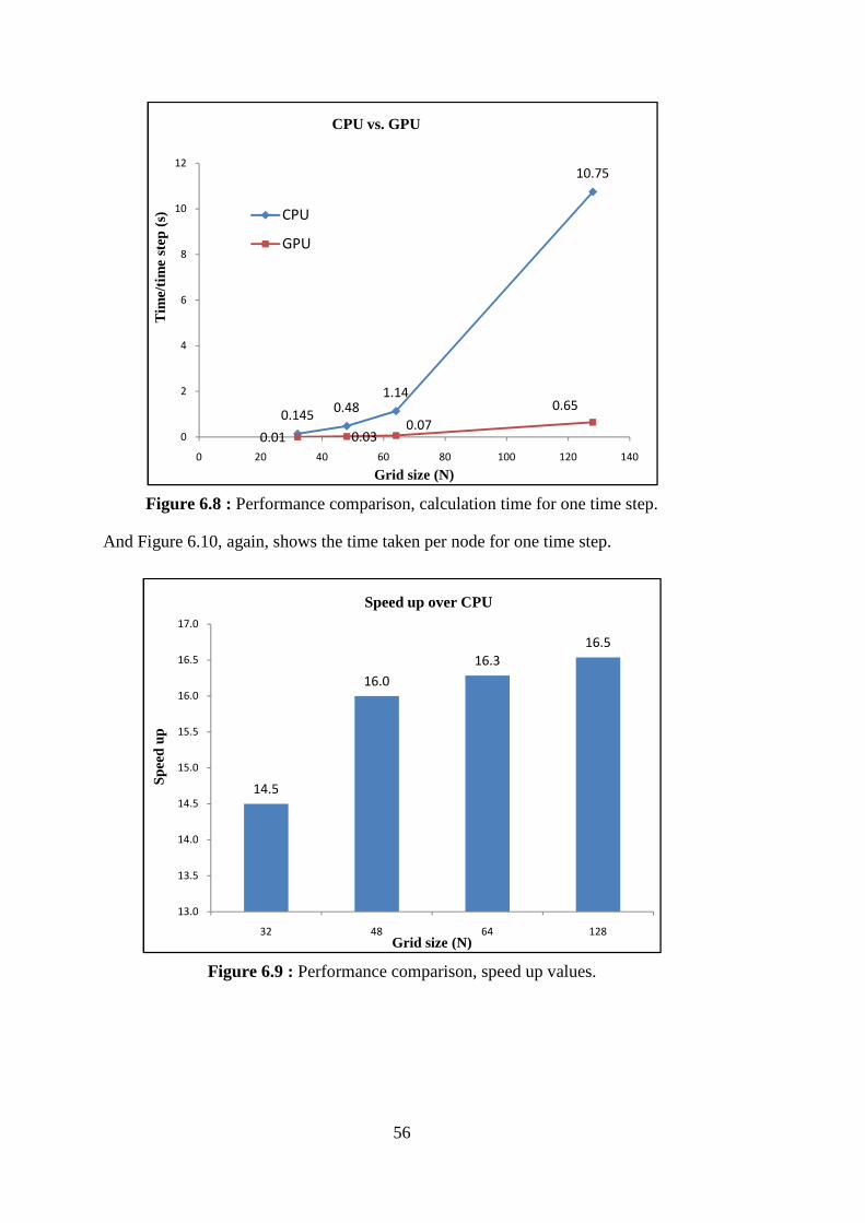
56
Figure 6.8 : Performance comparison, calculation time for one time step.
And Figure 6.10, again, shows the time taken per node for one time step.
Figure 6.9 : Performance comparison, speed up values.
0.1450.48
1.14
10.75
0.01 0.030.07
0.65
0
2
4
6
8
10
12
0 20 40 60 80 100 120 140
Tim
e/tim
e st
ep (
s)
Grid size (N)
CPU vs. GPU
CPU
GPU
14.5
16.0
16.3
16.5
13.0
13.5
14.0
14.5
15.0
15.5
16.0
16.5
17.0
32 48 64 128
Spe
ed u
p
Grid size (N)
Speed up over CPU

57
Figure 6.10 : Performance comparison, time taken per node.
Moreover, Figure 6.11 shows the timing breakdown of the GPU code for one time
step in the case of the 1283 mesh. It is clear that solutions of linear systems constitute
the most time consuming part in the code. In addition, since the filtering scheme also
generates cyclic tridiagonal systems, a remarkable portion of the filtering part
requires solutions of similar cyclic tri-diagonal systems. This emphasizes the need
for an efficient cyclic tridiagonal solver which may lead to much higher speedups of
GPU codes over a single CPU.
Figure 6.11 : Timing breakdown of one time step for 1283 mesh on GPU.
44.25
43.40
43.49 51.26
3.05 2.71 2.67 3.10
0.00
10.00
20.00
30.00
40.00
50.00
0.00 0.50 1.00 1.50 2.00
Tim
e p
er
no
de
(x
10
-7)
Total node number (x106)
Time per node for CPU and GPU
CPU
GPU
37%
20%
18%
12%
12%
Linear systems
Right sides
Solution vec.
Filtering
Other kernels

58
6.3 IBM Test Case - Flow Around a Square Cylinder
Fluid flow around bluff bodies is one of the most encountered flow problems in
various engineering fields. It has many practical applications in terms of CFD. One
of the main characteristics of this type of flows is the flow separation taking place in
the considerable portion of the surface. Thus, in turn, it leads to a remarkable wake
region which is characterized mainly by the shedding vortices from upper and lower
sides of the body. Depending on the flow system, this wake region may presents
some benefits like enhanced heat and mass transfer, but at the same time it may
cause some tiresome issues such as unwanted vibrations. Therefore, predicting the
wake region accurately is quite important. Most of the researches focused on the
flows around circular cylinder in the past [93]. Another important bluff body is
square cylinder. The flow around a square cylinder is similar to the circular cylinder
case in some ways. Nonetheless, it has also important differences in comparison with
circular cylinder. The square cylinder has fixed seperation points on either leading or
trailing edges in contrast to the circular cylinder. Moreover, generated wake
immediately after the square cylinder is wider than that of the circular cylinder. As a
result of this, the region covered by formation of the Karman vortices is much longer
and broader in the square cylinder case. Various flow regimes are encountered in the
flow past a square cylinder depending on the Reynolds number that is defined in
terms of free stream velocity, cylinder dimension and kinematic viscosity. If the
Reynolds number is below or about the unity, then no seperation is observed at the
surface of the cylinder. While the Reynolds number increases, the flow starts to
seperate first at the trailing edges and constitutes a closed, steady recirculation region
immediately behind the cylinder. If the Reynolds number is increased further, it
reaches a critical value (Rec) in which a periodic vortex shedding known as von
Karman vortex street appears in the wake region. Researchers give different values
for the critical reynolds number. Okajima [94] has performed an experimental study
for the rectangular cylinders and specifies an approximate value (Rec ≈ 70) for the
critical Reynolds number. Another experimetal study may be found in . Other values
given for the Rec are 53 in [95], 51 in [96]. Transition from the steady state to the
unsteady state is realized at this Reynolds number. Then if the Reynolds number is
further increased, the flow around a square cylinder makes a transition to three
dimensionality beyond a certain critical Reynolds number. There is not an exact

59
value for this critical Reynolds number, rather generally an interval is given for this
Reynolds number. In [97] it is said that transition to three dimensionality in the wake
of a square cylinder takes place in the limit between 150 and 175 of Reynolds
number. Similarly, [98] also gives the critical Reynolds number for the transition to
three dimesionality as �� = 162 ∓ 12.
In this study, simulation of the flow around a square cylinder is applied in order to
evaluate the IBM on GPU for the Reynolds numbers between 100 and 300. As
mentioned in the section involving the used numerical methods throughout this
thesis, sixth-order compact central finite difference schemes are utilized for both first
and second spatial derivatives for the discretization of the incompressible Navier-
Stokes equations.
Flow domain of this test case and applied boundary conditions are given in Figure
6.12. The square cylinder is placed between � = 6, � = 7iG�� = 5.85, � = 6.85.
Side length of the cylinder is » = 1, and its height is taken as 3.875». Values of the
dimensions in streamwise, stream-normal and spanwise directions are given in Table
6.3
Figure 6.12 : Immersed boundary flow domain and boundary conditions.
Table 6.3 : Dimensions of the flow domain.
X1/D Y1/D Z1/D
25.5 12.7 3.875

60
At the inlet, applied boundary conditions are = �R, � = # = 0 and �- ��⁄ = 0.
At the outlet, boundary conditions are � ��⁄ = �� ��⁄ = �# ��⁄ = 0 and - = 0.
Moreover, periodic boundary conditions are imposed to the crosswise and spanwise
boundaries.
Uniform grids are used for the computations of this test case. Total node numbers
along each Cartesian coordinate (x, y, z) are 384x192x32 nodes respectively. In
vortex dominated flow fields, It is quite important to calculate not only the region
near the body but also the wake region accurately. This is also another factor for the
usage of high-order compact scheme that has high accuracy and low numerical
dissipation in the region far from the immersed boundary. In this respect, using high-
order compact scheme also gives an opportunity to apply the uniform grid
throughout the flow domain. As a result, generated grid becomes coarser in the
vicinity of immersed boundary but fine enough to reach accurate results in terms of
whole flow domain. In Table 6.4 below, ∆� values which shows the first node
distance from the solid body for various studies in literature and present study are
indicated. The table also gives numerical methods used for the mentioned studies.
Table 6.4 : First node distance from the body.
Studies ∆� Method
Sohankar et al. [96] 0.004 Finite volume method.
2nd-3rd order in space.
Sharma and Eswaran [99] 0.01 Finite volume method.
2nd order in space.
Sahu et al. [100] 0.01 Finite volume method.
2nd order in space.
Singh et al. [101] 0.007 Finite volume method.
2nd order in space.
Sen et al. [102] 0.001 Finite element method
Present 0.066

61
As it is seen on the table, distance of the first node to the body in this study is at least
five times higher in comparison to others.
In the context of this study, Figure 6.13 shows the instantaneous streamlines and the
velocity contours of the flow domain for �� = 100. Form of the antisymmetric
wake flow, called as von Karman vortex street, can be seen evidently. As may be
seen in Figure 6.13, with the purpose of describing the characteristic of immersed
boundary method, these illustrations do not involve a square cylinder in the flow
domain as an object, but flow behaves just like there is one.
a
b
Figure 6.13 : a) Instantaneous streamlines, b) � velocity contours of the flow domain for Re =100.
Moreover, Figure 6.14, through a-h, depicts instantaneous streamlines in the vicinity
of square cylinder for a full vortex shedding cycle at �� = 100. In Figure 6.14, there
are also coreesponding images below the each phase of the cycle, showing the results
of another computational study [99]. With its eight consecutive frames Figure 6.14
covers a vortex shedding period. Centers and saddles related to vortex shedding are
also indicated in the figure. In addition, the process of instantaneous ‘alleyways’
mentioned in [103] is also demonsrated in the figure. In this process, fluid is sucked

62
into the recirculation region from both top and bottom of the cylinder succesively
through the “alleyways”.
a b
c d
Figure 6.14 : Instantaneous streamlines in the vicinity of square cylinder for a full avortex shedding cycle, Re = 100 (above: Present study, below: Sharma aand Eswaran [99]).

63
e f
g h
Figure 6.14 (continued) : Instantaneous streamlines in the vicinity of square acylinder for a full vortex shedding cycle, Re = 100 a(above: Present study, below: Sharma and Eswaran [99]).
As an example two of these alleyways are shown by the red arrows in Figure 6.14
b,e. For instance, looking at the figure, it can be seen that, the period begins with a
vortex maturing and shedding from lower side of the cylinder. At the same time,
during this interval, fluid is constantly sucked into the recirculation region from the
upper side . After the vortex sheds, then the same process is starting again but with
the opposite sides. This time vortex matures and sheds from the upper side of the
cylinder, and the fluid is sucked into the recirculation region from the lower side.

64
In addition, Figure 6.15 a-h gives the u velocity contours(above) and corresponding
pressure contours (below) for the same cycle presented in Figure 6.14.
Figure 6.15 : U velocity and pressure contours for a full vortex shedding cycle, Re = 100.
a b
c d
f e

65
Figure 6.15 (continued) : U velocity and pressure contours for a full vortex ishedding cycle, Re = 100.
Moreover, Figure 6.16 shows a comparison of the recirculation length defined as the
streamwise distance from the base of the square cylinder to the re-attachment point
on the wake centerline.
Figure 6.16 : Comparison of Lr. (Yoon et al. [104], Sharma and Eswaran [99], aRobichaux et al. [98])
1
1.5
2
90 100 110 120 130 140 150 160 170 180 190 200 210
Lr/
D
Re
Yoon et al. (2010)
Sharma and Eswaran (2004)
Robichaux et al. (1999)
Present
g h

66
The figure shows that the obtained recirculation lengths are in good agreement with
the results of other computational studies [98, 99, 104].
Strouhal number is also an important non-dimensional parameter giving the
information about the vortex shedding frequency of the flow and defined as:
¢� = H»�R (6.5)
Here, H, »and �Rstand for shedding frequency, cylinder dimension and free stream
velocity respectively. Shedding frequency may be obtained by appliying fast fourier
transform (FFT) to the lift coefficient or drag coefficient signals. Figure 6.17, as a
result of a FFT implementation, shows the power spectrum of Cl and Cd respectively.
As the figure indicates, while lift coefficient oscillates at the shedding frequency,
drag coefficient oscillates with twice the shedding frequency.
Figure 6.17 : Power spectrum of Cl (left) and Cd (right) for Re = 100.
In addition, Table 6.5 shows a comparison made between various previous studies
and the present one in terms of Strouhal number for �� = 100. As it may be seen
from the table, obtained value for St is quite consistent with other studies. The
biggest difference between the present value and the others is less than 1.5%. As an
addition to these Table 6.6 and Figure 6.18 indicate the comparisons of different
studies in terms of variation of Strouhal number with Reynolds number. It is
observed in the figure that obtained Strouhal number values in this study play along
with the results of other studies. If we look at the Figure 6.18 in a broad sense, it can
be seen that while the St values for �� = 100 and �� = 150 are clustered in a
narrower band, the values for the Reynolds number higher than 150 exhibit a more
discrete behaviour.
0
0.2
0.4
0.6
0.8
1
0 0.2 0.4 0.6 0.8 1
P
f
0
0.2
0.4
0.6
0.8
1
0 0.2 0.4 0.6 0.8 1
P
f

67
Table 6.5: Comparison of Strouhal numbers ifor �� = 100.
Studies St
Sohankar et al. [96] 0.146
Sharma and Eswaran [99] 0.148
Sahu et al. [100] 0.148
Singh et al. [101] 0.147
Sen et al. [102] 0.145
Present 0.146
Table 6.6: Comparison for the variation of Strouhal number with Re.
Re = 100 Re = 150 Re = 200 Re = 250 Re = 300
Okajima (exp.) [94] 0.142 0.143 0.145 0.144 0.145
Sen et al. [102] 0.145 0.160
Singh et al. [101] 0.147 0.156 0.143 0.133
Sharma and Esweran [99] 0.148 0.160
Saha et al. [97] 0.15 0.165 0.161 0.146 0.130
Sohankar et al. [105] 0.165 0.160 0.159 0.153
Robichaux et al. [98] 0.164 0.155
Sohankar et al. [96] 0.146 0.165
Franke et al. [106] 0.157 0.146 0.130
Davis et al. [107] 0.164 0.176
Present 0.146 0.161 0.158 0.156 0.155

68
In this context, it may be useful to remember that the flow around a square cylinder
makes a transition to three dimensionality beyond a certain critical Reynolds number.
There is not an exact value for this critical Reynolds number, rather generally an
interval is given for this Reynolds number. In [97] it is said that transition to three
dimensionality in the wake of a square cylinder takes place in the limit between 150
and 175 of Reynolds number. Similarly, [98] also gives the critical Reynolds number
for the transition to three dimesionality as �� = 162 ∓ 12. Therefore, three
dimensional effects may give some hints about the discreteness of St values for the
Re values higher than 150 in Figure 6.18.
Figure 6.18 : Variation of Strouhal number with Reynolds number. Mentioned studies: Okajima [94], Sen et al. [102], Singh et al. [101], Sharma and Eswaran [99], Saha et al. [97], Sohankar et al. [105], Robichaux et al. [98], Sohankar et al. [96], Franke et al. [106], Davis et al. [107].
Furthermore, because the no-slip boundary condition is not enforced strictly on the
body during the solution process, this condition is satisfied approximately.
Consequently, penetration of some streamlines into the immersed boundary may
occur as shown in Figure 6.14. As a result of this, although the wake region and
vortex shedding are simulated accurately, this issue somewhat deteriorates the force
calculations. Therefore, RMS of lift coefficients and time averaged drag coefficients
may be seen in Table 6.7 together with the other studies for Re = 100. It may also be
0.10
0.11
0.12
0.13
0.14
0.15
0.16
0.17
0.18
50 100 150 200 250 300 350
St
Re
Re vs. St
Okajima (experiment)
Sen et al.
Singh et al.
Sharma and Esweran
Saha et al.
Sohankar et al. (1999)
Robichaux et al.
Sohankar et al. (1998)
Franke et al.
Davis et al.
Present 3D

69
seen from the table Clrms value deviates much more than Cdave value. While Clrms
differs from the nearest value by more than 25%, this ratio for the Cdave is about 5%.
The same trend is observed for the various Reynolds numbers, those results are
indicated in Figure 6.19 and Figure 6.20. Likewise, drag coefficient exhibits the
similar pattern with other studies, whereas lift coefficient indicates more discrepancy
in comparison with drag coefficient.
Table 6.7: Comparison of Clrms and Cdave.
Study Clrms Cdave
Sharma and Eswaran [99] 0.19 1.49
Sahu et al. [100] 0.19 1.50
Singh et al. [101] 0.16 1.52
Sen et al. [102] 0.19 1.53
Saha et al. [97] 0.12 1.50
Present 0.26 1.41
Figure 6.19 : RMS of lift coefficients for the various Reynolds numbers.
0
0.2
0.4
0.6
0.8
1
50 100 150 200 250 300
CL r
ms
Re
Present
Sharma and Eswaran
Sahu et al.
Singh et al.
Sen et al.
Saha et al.
Sohankar et al.

70
Figure 6.20 : Time averaged drag coefficients for the various Reynolds numbers.
Generally speaking, solution process of the Poisson equation takes the vast majority
of the running time for one time step. Therefore, performance of the solution process
of this equation affects directly the overall performance of the incompressible flow
solver. Figure 6.21 shows the timing breakdown of one time step in the solution of
incompressible Navier-Stokes equations for the mesh consisting of 2x10⁶ nodes in
total.
Figure 6.21 : Timing breakdown of one time step.
1.3
1.4
1.5
1.6
1.7
1.8
50 100 150 200 250 300
Cd a
ve
Re
Present
Sharma and Eswaran
Sahu et al.
Singh et al.
Sen et al.
Saha et al.
Sohankar et al.
Robichaux et al.
0%
10%
20%
30%
40%
50%
60%
70%
80%
90%
100%
Poisson
Solution
Other parts

71
It may be obviously realized that, Poisson equation solution is the most decisive part
of all in terms of general performance. If we go further in analyzing the timing
breakdown of the relevant parts of the code, we can come up with the Figure 6.22.
Figure 6.22 : Timing breakdown of CG iterative solver.
This figure, like the previous one, also indicates a timing breakdown of a certain part
in the code in which conjugate gradient iterative solver takes place. The figure shows
time consuming percentages of each part for one iteration. It may also noted from the
figure that sparse matrix-vector multiplication is the most time consuming section of
the iterative process (≈75%). Currently, there is also a CUDA library in order to
handle sparse matrix and vector operations on CUDA enabled devices. Name of the
library is CUSPARSE [108]. Therefore one alternative is to utilize this library to
make the sparse matrix-vector multiplications in the solution process of Poisson
equation and the result indicated in Figure 6.22 is obtained by utilizing the
CUSPARSE library. In this respect, Figure 6.23 presents sparse matrix-vector
multiplication performance of CUSPARSE library.
0%
10%
20%
30%
40%
50%
60%
70%
80%
90%
100%
SpMV
daxpy
ddot
dscal

72
Figure 6.23 : SpMV performance of CUSPARSE library.
These values in the figure are obtained for a sparse matrix of standard 7 point
Poisson stencil with different total node numbers. CUSPARSE library can use
different sparse matrix format, such as coordinate (COO), compressed sparse row
(CSR) and compressed sparse column format (CSC). Presented values in Figure 6.23
are obtained by using CSR format. Instead of CSR format, a different storage format
also may be applied. In this study, ELLPACK format explained in section 3.5 is
exploited for the sparse matrix-vector multiplication. Written custom kernel
involving ELLPACK gives considerably better performance in comparison with
previously mentioned CUSPARSE library. Figure 6.24 shows this comparison for
the sparse matrix-vector multiplication for the cases with different total nodes. As it
may be seen in the figure ELLPACK format based kernel achieves approximately
3.5x speed ups over CUSPARSE library for the different grids.
In addition, constituted conjugate gradient iterative solver which uses ELLPACK
format is compared with the performance values in another GPU application from
literature [60]. In [60], conjugate gradient solver of CUSP library is used for the
solution of sparse linear systems, and a performance comparison between a GPU
(CUSP) and a CPU implementation is presented for the solution of sparse linear
systems.
0
0.002
0.004
0.006
0.008
0.01
0.012
0.014
0.016
0.018
0 1 2 3 4
Tim
e (
s)
Total node number (x106)
SpMV with CUSPARSE

73
Figure 6.24 : Performance comparison of CUSPARSE and ELLPACK.
CUSP is an open-source library for sparse linear algebra and graph computations on
CUDA [109]. Used CPU and GPU in that study are Intel Xeon X5650 and Tesla
C2050 respectively. Figure 6.25 shows this comparison for the solution of sparse
linear systems. Systems in this comparison are formed by the use of general 5-point
Poisson stencil. As it also may be seen in the figure present application of conjugate
gradient solver gives approximately 3 times better performance in comparison with
the application of CUSP library on the GPU. As a consequence of this performance
improvement, weight of the sparse matrix-vector multiplication in the conjugate
gradient algorithm decreases considerably. The final status of the timing breakdowns
may be seen in Figure 6.26. Figure 6.26 a and b shows the timing breakdowns of
incompressible flow solver and conjugate gradient iterative solver respectively.
Although, there is a reduction in percentage of the Poisson solver, it still has a share
of 86% and dominates the solution time heavily. Therefore, any further improvement
in the solution of Poisson equation can affect the performance of the GPU directly.
0
0.002
0.004
0.006
0.008
0.01
0.012
0.014
0.016
0.018
0 1 2 3 4
Tim
e (
s)
Total node number (x106)
CUSPARSE
ELLPACK

74
Figure 6.25 : Time comparison for the solution of sparse linear systems.
a
b
Figure 6.26 : Timing breakdown of incompressible solver and CG iterative solver after the use of ELLPACK form.
0
50
100
150
200
250
300
350
400
0.5 1 1.5 2 2.5 3 3.5 4
Tim
e (s
)
Total node number (x106)
CPU
GPU(cusp)
GPU (ELLPACK)
0%
10%
20%
30%
40%
50%
60%
70%
80%
90%
100%
Poisson
Solution
Other parts
0%
10%
20%
30%
40%
50%
60%
70%
80%
90%
100%
SpMV
daxpy
ddot
dscal

75
7. CONCLUSIONS
Purpose of this study is to test and apply some numerical tools, used in CFD, to GPU
that is coming to the forefront as a powerful computing device in recent years.
Applied numerical tools, a sixth-order compact scheme, a tenth-order filtering and
immersed boundary method, also attract a great deal of attention for the flow
simulations involving complex features and turbulent regime. A successful
incorporation of effective numerical methods and competent computing machines,
like GPU, may give rise to impressive progress in CFD.
With this object in mind, several applications are realized on the GPU in order to
analyze the real potential of this combination. Uniform grids are used for all test
cases. In vortex dominated flow fields, it is quite important to calculate not only the
region near the body but also the wake region accurately. This is also another factor
for the usage of high-order compact scheme that has high accuracy and low
numerical dissipation in the region far from the boudaries. In this respect, using high-
order compact scheme also gives an opportunity to apply the uniform grid
throughout the flow domain. As a result, generated grid becomes coarser in
comparison with the standard grid stretching approach in the vicinity of immersed
boundary but fine enough to reach accurate results in terms of whole flow domain.
Therefore, in first place, implementation of a high-order compact finite difference
scheme on a GPU is performed for the solution of some basic fluid dynamics
problems. A sixth-order compact central scheme and a tenth-order filtering scheme
are utilized in the solution of two example problems: advection of a vortical
disturbance and the temporal mixing layer. As a result of periodic boundary
conditions applied for both problems, the compact scheme and the filtering scheme
generate cyclic tridiagonal linear systems. In the CPU implementation which is
compared with the GPU code, these linear systems are solved efficiently by using
LAPACK/BLAS library, whereas the GPU code utilizes the inverse of the coefficient
matrix to solve the same linear system, resulting a faster but relatively inefficient
computation. Therefore, as the mesh size gets bigger, allocated time for solutions of

76
the linear systems increases remarkably for the GPU implementation. In this context,
for the finest mesh, 42% of the operating time is consumed to solve cyclic tridiagonal
linear systems. This shows that an improved solver for the solution of these relatively
small sized cyclic tridiagonal systems would further increase speedup of the GPU
implementation over the CPU implementation. In addition, shared memory which
has much lower latency values than the global memory is utilized in order to avoid
non-coalescing memory accessing. Currently, speedups between 9x–16.5x are
achieved on GPU compared to CPU computations.
It is concluded that, compact-finite-difference schemes on uniform Cartesian meshes
for the solution of CFD problems can achieve excellent speedup when implemented
on a GPU. As they require repeated solution of a relatively small cyclic tridiagonal
system with constant coefficients and multiple right-hand sides, further speedup is
possible with an appropriate solver for the specific structure of the linear system.
Furthermore, another test case involving immersed boundary method is also utilized.
Incompressible Navier-Stokes equations are solved on a Cartesian mesh with the
purpose of simulating the flow around a square cylinder. A direct forcing approach is
utilized for the immersed boundary method applied in this problem. In this approach,
the forcing term is inserted to the momentum equation in order to ensure the proper
boundary velocity value on the surface of immersed body. Again, a sixth-order
compact central scheme is used for the discretization of spatial derivatives and the
solution procedures related to compact scheme is the same as described shortly
before. Time advancement is ensured with the use of second-order Adams-Bashforth
scheme. Besides, a conjugate gradient iterative method is incorporated on GPU for
the solution of Poisson equation. In this context, two different approach are tested
for sparse matrix-vector multiplication which is the most decisive process in the
conjugate gradient iterative solver. First approach tested includes CUSPARSE sparse
matrix and vector operations library that utilizes the CSR format for the sparse
matrix. The second approach is a written custom kernel which implements
ELLPACK format for the saparse matrix. As a result, it is found that ELLPACK
format is more efficient for the problem dealt with. In addition to this, it provides an
opportunity for accessing the memory in a coalesced way. Within this scope, one
thing should also be added that shared memory is exploited for conjugate gradient
method in sparse-matrix vector multiplication too. Immersed boundary effects are

77
provided by inserting a force term directly to the momentum equation. Thus, with
this suitably designed direct forcing term, a square cylinder is represented on a
Cartesian mesh. Results are obtained for the Reynolds number range of 100-300.
Obtained streamline structure for one cycle of vortex shedding at �� = 100 is
presented to show the capability of the method to simulate the wake region of the
cylinder. Moreover, comparisons with other studies are exhibited in terms of
Strouhal numbers for various Reynolds numbers. It is seen that present
implementation simulates the wake region and vortex shedding accurately, but is not
very successful at estimating the force coefficients. Due to approximately satisfied
no-slip boundary condition, stremlines may penetrate into the immersed body. In
turn, this causes to degraded results especially for the lift coefficient. Furthermore, a
comparison is made regarding the performance of the present GPU application. Since
solving the sparse linear systems efficiently is the most decisive factor in terms of the
performance, a comparison is performed between present implementation and other
GPU and CPU applications for the sparse linear system solutions. As a consequence,
about 3x and 20x speedups are achieved in comparison with GPU and CPU
respectively.
Generally, GPUs obviously have pretty much potential as parallel computing
devices. With accordingly coded algorithms and the advancements in numerical tools
that can exploit the GPUs strength effectively, they may become the most influential
assistants of researchers in dealing with large, complex fluid flow problems.
7.1 Future Works
Some further improvements in terms of obtained results and performance can be
achieved by incorporating some future works in to the present one. First of all,
GPGPU market develops steadily, brand-new GPUs come onto the market just every
several years. Even only with one of the latest GPU, one can reach higher
performance values by doing slight modifications to constituted code here. Apart
from this, future work may include the followings:
- Necessary modifications for porting the code to multi-GPU environment.
- Constitution of more efficient lineer solvers for cyclic tridiagonal systems.

78
- Incorporation of a spectral solver instead of conjugate gradient approach for
Poisson equation.
- Grid clustering in the vicinity of an immersed boundary for more accuracy.

79
REFERENCES
[1] Lele, S. K. (1992). Compact finite-difference schemes with spectral-like resolution, Journal of Computational Physics, 103(1), 16-42.
[2] Visbal, M. R. & Gaitonde, D. V. (2002). On the use of higher-order finite-difference schemes on curvilinear and deforming meshes, Journal of Computational Physics, 181(1), 155-185.
[3] Hirsh, R. S. (1975). Higher-order accurate difference solutions of fluid mechanics problems by a compact differencing technique, Journal of Computational Physics, 19(1), 90-109.
[4] Weinan, E. & Liu, J. G. (1996). Essentially compact schemes for unsteady viscous incompressible flows. Journal of Computational Physics, 126(1), 122-138.
[5] Gamet, L., Ducros, F., Nicoud, F. & Poinsot, T. (1999). Compact finite difference schemes on non-uniform meshes. Application to direct numerical simulations of compressible flows, International Journal for Numerical Methods in Fluids, 29(2), 159-191.
[6] Mahesh, K. (1998). A family of high order finite difference schemes with good spectral resolution, Journal of Computational Physics, 145(1), 332-358.
[7] Meitz, H. L. & Fasel, H. F. (2000). A compact-difference scheme for the Navier-Stokes equations in vorticity-velocity formulation, Journal of Computational Physics, 157(1), 371-403.
[8] Demuren, A. O., Wilson, R. V. & Carpenter, M. (2001). Higher-order compact schemes for numerical simulation of incompressible flows, part I: Theoretical development, Numerical Heat Transfer Part B-Fundamentals, 39(3), 207-230.
[9] Meinke, M., Schroder, W., Krause, E. & Rister, T. (2002). A comparison of second- and sixth-order methods for large-eddy simulations, Computers & Fluids, 31(4-7), 695-718.
[10] Nagarajan, S., Lele, S. K. & Ferziger, J. H. (2003). A robust high-order compact method for large eddy simulation, Journal of Computational Physics, 191(2), 392-419.
[11] Shukla, R. K., Tatineni, M. & Zhong, X. L. (2007). Very high-order compact finite difference schemes on non-uniform grids for incompressible Navier-Stokes equations, Journal of Computational Physics, 224(2), 1064-1094.
[12] Rizzetta, D. P., Visbal, M. R. & Morgan, P. E. (2008). A high-order compact finite-difference scheme for large-eddy simulation of active flow control, Progress in Aerospace Sciences, 44(6), 397-426.

80
[13] Boersma, B. J. (2011). A 6th order staggered compact finite difference method for the incompressible Navier-Stokes and scalar transport equations, Journal of Computational Physics, 230(12), 4940-4954.
[14] Visbal, M. R. & Gaitonde, D. V. (1999). High-order-accurate methods for complex unsteady subsonic flows, Aiaa Journal, 37(10), 1231-1239.
[15] Mittal, R. & Iaccarino, G. (2005). Immersed boundary methods, Annual Review of Fluid Mechanics, 37, 239-261.
[16] Peskin, C.S. (2002). The immersed boundary method, Acta Numerica, 11, 479-517.
[17] Peskin, C. S. (1972). Flow Patterns around heart valves - numerical method, Journal of Computational Physics, 10(2), 252-271.
[18] Liao, C. C., Chang, Y. W., Lin, C. A. & McDonough, J. M. (2010). Simulating flows with moving rigid boundary using immersed-boundary method, Computers & Fluids, 39(1), 152-167.
[19] Lei, Y. X., Wei, H. G. & Xing, Z. (2010). Large-eddy simulation of flows past a flapping airfoil using immersed boundary method, Science China-Physics Mechanics & Astronomy, 53(6), 1101-1108.
[20] Paravento, F., Pourquie, M. J. & Boersma, B. J. (2008). An immersed boundary method for complex flow and heat transfer, Flow Turbulence and Combustion, 80(2), 187-206.
[21] Seo, J. H. & Mittal, R. (2011). A high-order immersed boundary method for acoustic wave scattering and low-Mach number flow-induced sound in complex geometries, Journal of Computational Physics, 230(4), 1000-1019.
[22] Lai, M. C. & Peskin, C. S. (2000). An immersed boundary method with formal second-order accuracy and reduced numerical viscosity, Journal of Computational Physics, 160(2), 705-719.
[23] Goldstein, D., Handler, R. & Sirovich, L. (1993). Modeling a no-slip flow boundary with an external force-field, Journal of Computational Physics, 105(2), 354-366.
[24] Saiki, E. M. & Biringen, S. (1996). Numerical simulation of a cylinder in uniform flow: Application of a virtual boundary method, Journal of Computational Physics, 123(2), 450-465.
[25] Mohd-Yusof, J. (1997). Combined immersed boundaries/b-splines methods for simulations of flows in complex geometries. NASA Ames/Stanford University: CTR Annual Research Briefs.
[26] Fadlun, E. A., Verzicco, R., Orlandi, P. & Mohd-Yusof, J. (2000). Combined immersed-boundary finite-difference methods for three-dimensional complex flow simulations, Journal of Computational Physics, 161(1), 35-60.
[27] Zhang, N. & Zheng, Z. C. (2007). An improved direct-forcing immersed-boundary method for finite difference applications, Journal of Computational Physics, 221(1), 250-268.

81
[28] Ikeno, T. & Kajishima, T. (2007). Finite-difference immersed boundary method consistent with wall conditions for incompressible turbulent flow simulations, Journal of Computational Physics, 226(2), 1485-1508.
[29] Iaccarino, G. & Verzicco, R. (2003). Immersed boundary technique for turbulent flow simulations, Applied Mechanics Reviews, 56(3), 331-347.
[30] Kim, J., Kim, D. & Choi, H. (2001). An immersed-boundary finite-volume method for simulations of flow in complex geometries, Journal of Computational Physics, 171(1), 132-150.
[31] Tseng, Y. H. & Ferziger, J. H. (2003). A ghost-cell immersed boundary method for flow in complex geometry, Journal of Computational Physics, 192(2), 593-623.
[32] Balaras, E. (2004). Modeling complex boundaries using an external force field on fixed Cartesian grids in large-eddy simulations, Computers & Fluids, 33(3), 375-404.
[33] Yang, J. M. & Balaras, E. (2006). An embedded-boundary formulation for large-eddy simulation of turbulent flows interacting with moving boundaries, Journal of Computational Physics, 215(1), 12-40.
[34] Kim, D. & Choi, H. (2006). Immersed boundary method for flow around an arbitrarily moving body, Journal of Computational Physics, 212(2), 662-680.
[35] Owens, J. D., Luebke, D., Govindaraju, N., Harris, M., …. Purcell, T. J. (2007). A survey of general-purpose computation on graphics hardware, Computer Graphics Forum, 26(1), 80-113.
[36] Hagen, T. R., Lie, K. A. & Natvig, J. R. (2006). Solving the Euler equations on graphics processing units, Proceedings of the Sixth International Conference on Computational Science, Part IV, (pp. 220-227). United Kingdom: Reading, May 28-31.
[37] Brandvik, T. & Pullan, G. (2007). Acceleration of a two-dimensional Euler flow solver using commodity graphics hardware, Proceedings of the Institution of Mechanical Engineers Part C-Journal of Mechanical Engineering Science, 221(12), 1745-1748.
[38] Brandvik, T. & Pullan, G. (2008). Acceleration of a 3D Euler solver using commodity graphics hardware (AIAA Paper 2008-607), 46th AIAA Aerospace Sciences Meeting and Exhibit. Reno, USA: January 7-10.
[39] Elsen, E., LeGresley, P. & Darve, E. (2008). Large calculation of the flow over a hypersonic vehicle using a GPU, Journal of Computational Physics, 227(24), 10148-10161.
[40] Corrigan, A., Camelli, F. F., Lohner, R. & Wallin, J. (2011). Running unstructured grid-based CFD solvers on modern graphics hardware, International Journal for Numerical Methods in Fluids, 66(2), 221-229.

82
[41] Tolke, J. & Krafczyk, M. (2008). TeraFLOP computing on a desktop PC with GPUs for 3D CFD, International Journal of Computational Fluid Dynamics, 22(7), 443-456.
[42] Zhao, Y. (2008). Lattice boltzmann based PDE solver on the GPU, Visual Computer, 24(5), 323-333.
[43] Che, S., Boyer, M., Meng, J. Y., Tarjan, D., Sheaffer, J. W. & Skadron, K. (2008). A performance study of general-purpose applications on graphics processors using CUDA, Journal of Parallel and Distributed Computing, 68(10), 1370-1380.
[44] Rossinelli, D. & Koumoutsakos, P. (2008). Vortex methods for incompressible flow simulations on the GPU, Visual Computer, 24(7-9), 699-708.
[45] Wang, P., Abel, T. & Kaehler, R. (2010). Adaptive mesh fluid simulations on GPU, New Astronomy, 15(7), 581-589.
[46] Rossinelli, D., Bergdorf, M., Cottet, G. H. & Koumoutsakos, P. (2010). GPU accelerated simulations of bluff body flows using vortex particle methods, Journal of Computational Physics, 229(9), 3316-3333.
[47] Kampolis, I. C., Trompoukis, X. S., Asouti, V. G. & Giannakoglou, K. C. (2010). CFD-based analysis and two-level aerodynamic optimization on graphics processing units, Computer Methods in Applied Mechanics and Engineering, 199(9-12), 712-722.
[48] Xian, W. & Takayuki, A. (2011). Multi-GPU performance of incompressible flow computation by lattice Boltzmann method on GPU cluster, Parallel Computing, 37(9), 521-535.
[49] Hoffmann, K. A. & Chiang, S. T. (2000). Computational Fluid Dynamics (4th ed., Vol. 1). Vichita, USA: Engineering Education System.
[50] Ferziger, J. H. & Peric, M. (2002). Computational Methods for Fluid Dynamics. New york, USA: Springer-Verlag.
[51] Hoffmann, K. A. & Chiang, S. T. (2000). Computational Fluid Dynamics (4th ed., Vol. 3). Vichita, USA: Engineering Education System.
[52] Ekaterinaris, J. A. (2005). High-order accurate, low numerical diffusion methods for aerodynamics, Progress in Aerospace Sciences, 41(3-4), 192-300.
[53] Laizet, S. & Lamballais, E. (2009). High-order compact schemes for incompressible flows: A simple and efficient method with quasi-spectral accuracy, Journal of Computational Physics, 228(16), 5989-6015.
[54] Uzun, A., Blaisdell, G. A. & Lyrintzis, A. S. (2004). Application of compact schemes to large eddy simulation of turbulent jets, Journal of Scientific Computing, 21(3), 283-319.
[55] Gaitonde, D. V. & Visbal, M. R. (2000). Pade-type higher-older boundary filters for the Navier-Stokes equations, Aiaa Journal, 38(11), 2103-2112.

83
[56] Beyer, R. P. & Leveque, R. J. (1992). Analysis of a one-dimensional model for the immersed boundary method, Siam Journal on Numerical Analysis, 29(2), 332-364.
[57] Unverdi, S. O. & Tryggvason, G. (1992). A front-tracking method for viscous, incompressible, multi-fluid flows, Journal of Computational Physics, 100(1), 25-37.
[58] Zhu, L. D. & Peskin, C. S. (2003). Interaction of two flapping filaments in a flowing soap film, Physics of Fluids, 15(7), 1954-1960.
[59] Stockie, J. M. & Wetton, B. R. (1999). Analysis of stiffness in the immersed boundary method and implications for time-stepping schemes, Journal of Computational Physics, 154(1), 41-64.
[60] Layton, S. K., Krishnan, A. & Barba, L. A. (2011). cuIBM – A GPU-accelerated immersed boundary method, International Conference on Parallel Computational Fluid Dynamics, Barcelona, Spain: May 16-20.
[61] Verzicco, R., Mohd-Yusof, J., Orlandi, P. & Haworth, D. (2000). Large eddy simulation in complex geometric configurations using boundary body forces, Aiaa Journal, 38(3), 427-433.
[62] Ferziger, J. H. & Peric, M. (2002). Computational Methods for Fluid Dynamics. Berlin: Springer-Verlag.
[63] Bell, N. & Garland, M. (2009). Implementing sparse matrix-vector multiplication on throughput-oriented processors, Conference on High Performance Computing, Networking, Storage and Analysis, Portland, Oregon, USA: November 14-20.
[64] Vázquez, F., Ortega, G., Fernández, J. J. & Garzón E. M. (2010). Improving the performance of the sparse matrix vector product with GPUs, The 10th IEEE International Conference on Computer and Information Technology, Bradford, UK: June 29-July 01.
[65] Hwu, W., Keutzer, K. & Mattson, T. G. (2008). The concurrency challenge, IEEE Design and Test of Computers, 25(4), 312-320.
[66] Kirk, D. B. & Hwu, W. (2010). Programming Massively Parallel Processors. Burlington, USA: Morgan Kaufmann.
[67] Trapnell, C. & Schatz, M. C. (2009). Optimizing data intensive GPGPU computations for DNA sequence alignment, Parallel Computing, 35(8-9), 429-440.
[68] Shi, H. X., Schmidt, B., Liu, W. G. & Muller-Wittig , W. (2009). Accelerating error correction in high-throughput short-read DNA sequencing data with CUDA, 2009 Ieee International Symposium on Parallel & Distributed Processing (Vol. 1-5, pp. 1546-1553). Rome, Italy: May 25-29
[69] Klockner, A., Warburton, T., Bridge, J. & Hesthaven, J. S. (2009). Nodal discontinuous Galerkin methods on graphics processors, Journal of Computational Physics, 228(21), 7863-7882.

84
[70] Ma, W. J. & Agrawal, G. (2009). A compiler and runtime system for enabling data mining applications on GPUs, Acm Sigplan Notices, 44(4), 287-288.
[71] Sintorn, E. & Assarsson, U. (2008). Fast parallel GPU-sorting using a hybrid algorithm, Journal of Parallel and Distributed Computing, 68(10), 1381-1388.
[72] McGraw, T. & Nadar, M. (2007). Stochastic DT-MRI connectivity mapping on the GPU, Ieee Transactions on Visualization and Computer Graphics, 13(6), 1504-1511.
[73] Stone, S. S., Haldar, J. P., Tsao, S. C., Hwu, W. M. W., …. Liang, Z. P. (2008). Accelerating advanced MRI reconstructions on GPUs, Journal of Parallel and Distributed Computing, 68(10), 1307-1318.
[74] Maintz, S., Eck, B. & Dronskowski, R. (2011). Speeding up plane-wave electronic-structure calculations using graphics-processing units, Computer Physics Communications, 182(7), 1421-1427.
[75] Harvey, M. J. & De Fabritiis, G. (2009). An Implementation of the Smooth Particle Mesh Ewald Method on GPU Hardware, Journal of Chemical Theory and Computation, 5(9), 2371-2377.
[76] Harris, M. J. (2004) Fast Fluid Dynamics Simulation on the GPU, in R. Fernando (editor), GPU Gems (pp. 637-665). Boston: Pearson Education.
[77] Crane, K., Llamas, I. & Tariq, S. (2007) Real-time Simulation and Rendering of 3D Fluids, in H. Nguyen (editor), GPU Gems 3 (pp. 633-675). Boston: Pearson Education.
[78] Göddeke, D., Strzodka, R., Mohd-Yusof, J., McCormick, P., …. Turek, S. (2008). Using GPUs to improve multigrid solver performance on a cluster, International journal of Computational Science and Engineering, 4(1), 36-55.
[79] Kuznik, F., Obrecht, C., Rusaouen, G. & Roux, J. J. (2010). LBM based flow simulation using GPU computing processor, Computers & Mathematics with Applications, 59(7), 2380-2392.
[80] Asouti, V. G., Trompoukis, X. S., Kampolis, I. C. & Giannakoglou, K. C. (2011). Unsteady CFD computations using vertex-centered finite volumes for unstructured grids on graphics processing units, International Journal for Numerical Methods in Fluids, 67(2), 232-246.
[81] Thibault, J. C. & Senocak, I. (2009), CUDA implementation of a Navier-Stokes solver on multi-GPU desktop platforms for incompressible flows (AIAA Paper 2009-758), 47th AIAA Aerospace Sciences Meeting and exhibit. Orlando, USA: January 5-8.
[82] Antoniou, A. S., Karantasis, K. I., …. Ekaterinaris, J. A. (2010). Acceleration of a finite-difference WENO scheme for large-scale simulations on many-core architectures (AIAA Paper 2010-525), 48th AIAA Aerospace Sciences Meeting and exhibit. Orlando, USA: January 4-7.

85
[83] Castonguay, P., Williams, D., Vincent, P., Lopez, M. & Jameson, A. (2011). On the development of a high-order, multi-GPU enabled, compressible viscous flow solver for mixed unstructured grids, 20th AIAA Computational Fluid Dynamics Conference, Honolulu, Hawaii: June 27-30.
[84] Url-1 <http://www.nvidia.com/docs/IO/56483/Tesla_C1060_boardSpec_ v03.pdf>, date retrieved 02.11.2012.
[85] Tutkun, B. & Edis, F. O. (2012). A GPU application for high-order compact finite difference scheme, Computers & Fluids, 55, 29-35.
[86] Goddeke, D. & Strzodka, R. (2011). Cyclic reduction tridiagonal solvers on GPUs applied to mixed-precision multigrid, Ieee Transactions on Parallel and Distributed Systems, 22(1), 22-32.
[87] Zhang, Y., Cohen, J. & Owens, J. D. (2010). Fast tridiagonal solvers on the GPU, Ppopp 2010. Proceedings of the 2010 Acm Sigplan Symposium on Principles and Practice of Parallel Programming, (pp. 127-136). Bangalore, India: January 9-14.
[88] Url-2 <http://www.serc.iisc.ernet.in/facilities/ComputingFacilities/systems/ fermi/CUDA_C_Best_Practices_Guide.pdf>, date retrieved 02.11.2012.
[89] Url-3 <http://www.scribd.com/doc/49843063/CUDA-C-Programming-Guide>, date retrieved 02.11.2012.
[90] Lesieur, M., Staquet, C., Leroy, P. & Comte, P. (1988). The mixing layer and its coherence examined from the point of view of two-dimensional turbulence, Journal of Fluid Mechanics, 192, 511-534.
[91] Lesieur, M., Comte, P., Chollet, J. P. & Le Roy, P. (1987). Numerical simulation of coherent structures in free shear flows, NATO Advanced Research Workshop on Mathematical Modeling in Combustion and Related Topics, Lyon, France: April 27-30.
[92] Ozel, A. (2006). Computational fluid dynamics analysis of turbulent flows (Master's thesis). Istanbul Technical University, Graduate School of Science Engineering and Technology, İstanbul.
[93] Williamson, C. H. K. (1996). Vortex dynamics in the cylinder wake, Annual Review of Fluid Mechanics, 28, 477-539.
[94] Okajima, A. (1982). Strouhal numbers of rectangular cylinders, Journal of Fluid Mechanics, 123, 379-398.
[95] Kelkar, K. M. & Patankar, S. V. (1992). Numerical prediction of vortex shedding behind a square cylinder, International Journal for Numerical Methods in Fluids, 14(3), 327-341.
[96] Sohankar, A., Norberg, C. & Davidson, L. (1998). Low-Reynolds-number flow around a square cylinder at incidence: Study of blockage, onset of vortex shedding and outlet boundary condition, International Journal for Numerical Methods in Fluids, 26(1), 39-56.

86
[97] Saha, A. K., Biswas, G. & Muralidhar, K. (2003). Three-dimensional study of flow past a square cylinder at low Reynolds numbers, International Journal of Heat and Fluid Flow, 24(1), 54-66.
[98] Robichaux, J., Balachandar, S. & Vanka, S. P. (1999). Three-dimensional Floquet instability of the wake of square cylinder, Physics of Fluids, 11(3), 560-578.
[99] Sharma, A. & Eswaran, V. (2004). Heat and fluid flow across a square cylinder in the two-dimensional laminar flow regime, Numerical Heat Transfer Part A-Applications, 45(3), 247-269.
[100] Sahu, A. K., Chhabra, R. P. & Eswaran, V. (2009). Two-dimensional unsteady laminar flow of a power law fluid across a square cylinder, Journal of Non-Newtonian Fluid Mechanics, 160(2-3), 157-167.
[101] Singh, A. P., De, A. K., Carpenter, V. K., Eswaran, V. & Muralidhar, K. (2009). Flow past a transversely oscillating square cylinder in free stream at low Reynolds numbers, International Journal for Numerical Methods in Fluids, 61(6), 658-682.
[102] Sen, S., Mittal, S. & Biswas, G. (2011). Flow past a square cylinder at low Reynolds numbers, International Journal for Numerical Methods in Fluids, 67(9), 1160-1174.
[103] Perry, A. E., Chong, M. S. & Lim, T. T. (1982). The Vortex-Shedding Process Behind Two-Dimensional Bluff-Bodies, Journal of Fluid Mechanics, 116, 77-90.
[104] Yoon, D. H., Yang, K. S. & Choi, C. B. (2010). Flow past a square cylinder with an angle of incidence, Physics of Fluids, 22(4).
[105] Sohankar, A., Norberg, C. & Davidson, L. (1999). Simulation of three-dimensional flow around a square cylinder at moderate Reynolds numbers, Physics of Fluids, 11(2), 288-306.
[106] Franke, R., Rodi, W. & Schonung, B. (1990). Numerical-calculation of laminar vortex-shedding flow past cylinders, Journal of Wind Engineering and Industrial Aerodynamics, 35(1-3), 237-257.
[107] Davis, R. W., Moore, E. F. & Purtell, L. P. (1984). A Numerical-experimental study of confined flow around rectangular cylinders, Physics of Fluids, 27(1), 46-59.
[108] Url-4 <http://developer.download.nvidia.com/compute/cuda/3_2_prod/toolkit/ docs/ CUSPARSE_Library.pdf>, date retrieved 02.11.2012.
[109] Url-5 <http://code.google.com/p/cusp-library/>, date retrieved 02.11.2012.

87
APPENDICES
APPENDIX A: Fourier Error Analysis of Some Central Finite Difference
Schemes for First and Second Derivatives
In this appendix, Fourier error analyses of some central finite difference schemes are
presented below for the first and second derivatives. For the first derivative:
Fourth-order Pade scheme:
HALM} + 4HA} + HANM} = 3$HANM − HALM∆� ( (A.1)
C0HANJ = F3∗�@JD∆0�@D0w = F3∗�@JD∆0HA (A.2)
F3∗HA~�L@D∆0 + 4 + �@D∆0� = 3∆� ~�@D∆0 − �L@D∆0�HA (A.3)
�@D∆0 = cosZ3∆�\ + F|FGZ3∆�\ (A.4)
3∗∆� = 3|FGZ3∆�\2 + W�|Z3∆�\ (A.5)
Eight-order pentadiagonal compact scheme:
HAL&} + 16HALM} + 36HA} + 16HANM} + HAN&} = 1603 $HANM − HALM2∆� ( + 503 $HAN& − HAL&4∆� ( (A.6)
F3∗HA~�L@&D∆0 + 16�L@D∆0 + 36 + 16�@D∆0 + �@&D∆0�= �1603 $�@D∆0 − �L@D∆02∆� ( + 503 $�
@&D∆0 − �L@&D∆04∆� (�HA (A.7)
3∗∆� = 320|FGZ3∆�\ + 50sinZ23∆�\216 + 12W�|Z23∆�\ + 192cosZ3∆�\ (A.8)

88
Tenth-order pentadiagonal compact scheme:
HAL&} + 10HALM} + 20HA} + 10HANM} + HAN&}= 853 $HANM − HALM2∆� ( + 20215 $HAN& − HAL&4∆� ( + 15$HANe − HALe6∆� ( (A.9)
F3∗HA~�L@&D∆0 + 10�L@D∆0 + 20 + 10�@D∆0 + �@&D∆0�= �853 $�
@D∆0 − �L@D∆02∆� ( + 20215 $�@&D∆0 − �L@&D∆04∆� (
+ 15$�@eD∆0 − �L@eD∆06∆� (� HA
(A.10)
3∗∆� = 850|FGZ3∆�\ + 202sinZ23∆�\ + 2sinZ33∆�\600 + 60W�|Z23∆�\ + 600cosZ3∆�\ (A.11)
And for the second derivative:
Fourth-order Pade scheme:
HALM}} + 10HA}} + HANM}} = 12$HANM − 2HA + HALM∆�& ( (A.12)
−3∗&~�L@D∆0 + 10 + �@D∆0� = 12∆�& ~�@D∆0 − 2 + �L@D∆0� (A.13)
3∗&∆�& = 12 − 12W�|Z3∆�\5 + W�|Z3∆�\ (A.14)
Eight-order pentadiagonal compact scheme:
HAL&}} + 68823 HALM}} + 235823 HA}} + 68823 HANM}} + HAN&}}= 192023 $HANM − 2HA + HALM∆�& ( + 186023 $HAN& − 2HA + HAL&4∆�& (
(A.15)

89
−3∗& P�L@&D∆0 + 68823 �L@D∆0 + 235823 + 68823 �@D∆0 + �@&D∆0Q= 192023 $�@D∆0 − 2 + �L@D∆0∆�& (+ 186023 $�@&D∆0 − 2 + �L@&D∆04∆�& (
(A.16)
3∗&∆�& = 6384092 9~2 − 2W�|Z3∆�\� + 693092 9 Z2 − 2cosZ23∆�\\6117923 9 + W�|Z23∆�\ + Z68823 \cosZ3∆�\ (A.17)
Tenth-order pentadiagonal compact scheme:
HAL&}} + 66843 HALM}} + 179843 HA}} + 66843 HANM}} + HAN&}}= 106543 $HANM − 2HA + HALM∆�& ( + 207643 $HAN& − 2HA + HAL&4∆�& (+ 7943$HANe − 2HA + HALe9∆�& (
(A.15)
−3∗& P�L@&D∆0 + 66843 �L@D∆0 + 179843 + 66843 �@D∆0 + �@&D∆0Q= 106543 $�@D∆0 − 2 + �L@D∆0∆�& (+ 207643 $�@&D∆0 − 2 + �L@&D∆04∆�& (+ 7943$�
@eD∆0 − 2 + �L@eD∆09∆�& (
(A.16)
3∗&∆�&= ~½�r�er¾ �~1 − W�|Z3∆�\� + ~np¾Mer¾ �Z1 − cosZ23∆�\\ + ~ ¾½er¾�Z1 − cosZ33∆�\\r½½ne + W�|Z23∆�\ + pprne cosZ3∆�\ (A.17)

90

91
CURRICULUM VITAE
Name Surname: Bülent Tutkun
Place and Date of Birth: Istanbul / 1974
Address: Istanbul Teknik Üniversitesi, Uçak ve Uzay Bil. Fakültesi
E-Mail: [email protected]
B.Sc.: Astronautical Engineering
M.Sc.: Astronautical Engineering
Professional Experience and Rewards:
Research assistant in ITU, Faculty of Aeronautics and Astronautics since 2001.
List of Publications and Patents:
� Kurtulus, C., Baltaci, T., Ulusoy, M., Aydin, B. T., Tutkun, B . et al. (2007). ITU-pSAT I: Istanbul Technical University Student Pico-Satellite Program, 3rd International Conference on Recent Advances in Space Technologies, Istanbul, Turkey: June 14-16.
� Tutkun, B. & Meric, R. A. (2002). Comparison of turbulence models for transonic flow around an airfoil, Kayseri 4th National Aviation Symposium, Kayseri, Erciyes University: May 13-15.
� Tutkun, B. & Meric, R. A. (2001). Analysis of thermal flows around an airfoil in the canal with finite volume method and grid optimization, 12th National Mechanics Congress, Konya, Selcuk University: September 10-14.
PUBLICATIONS/PRESENTATIONS ON THE THESIS
� Tutkun B. & Edis F.O. (2012). A GPU application for high-order compact finite difference scheme, Computers & Fluids, 55, 29-35.
� Tutkun B. & Edis F.O. (2012). A GPU implementation for the direct-forcing immersed boundary method, 24th International Conference on Parallel Computational Fluid Dynamics, Atlanta, USA: May 21-25.

92