Embed Size (px)
Citation preview

The 18th Federal Forecasters Conference
Issues in Forecasting and the Environment April 21, 2011 at the Bureau of Labor Statistics
Sponsoring Agencies Bureau of Labor Statistics Bureau of Transportation Statistics Economic Research Service Internal Revenue Service International Trade Administration National Center for Education Statistics U.S. Census Bureau U.S. Department of Veterans Affairs U.S. Energy Information Administration U.S. Geological Survey U.S. Postal Service
Partnering Organization Research Program on Forecasting The George Washington University
www.federalforecasters.org

2011 Federal Forecasters Conference Papers and Proceedings
Announcement The 19th
Federal Forecasters Conference FFC2012
Will be held
September 27, 2012
In
Washington, DC

2011 Federal Forecasters Conference i Papers and Proceedings
Contents Announcements ........................................................................................................................... Inside Cover Table of Contents ........................................................................................................................................... i Editor Page ................................................................................................................................................... iii Federal Forecasters Consortium Board ........................................................................................................ iv Foreword ...................................................................................................................................................... vi Acknowledgements ..................................................................................................................................... vii 2011 Federal Forecasters Conference Forecasting Contest Winners ......................................................... viii 2009 Best Conference Paper Awards ........................................................................................................... ix Scenes from the Conference ......................................................................................................................... x
Morning Session
Panel Discussion ..................................................................................................................................... 1
Forecasting for Transportation, Energy, and the Environment Arthur Rypinski, U.S. Department of Transportation ............................................................................ 2
The Bureau of Labor Statistics Green Jobs Initiative (and Why We Are Not Doing Green Jobs Projections) Dixie Sommers, U.S. Department of Labor .......................................................................................... 2
Forecasting and Assessing Environmental Performance in a Non-Market Economy Joy Harwood and Skip Hyberg, U.S. Department of Agriculture ......................................................... 3
Concurrent Sessions I
Long Term Forecasts
Article Abstracts ................................................................................................................................... 11
Language Projections: 2010 to 2020 Hyon B. Shin and Jennifer M. Ortman, U.S. Census Bureau ............................................................... 13
Comparing Government Forecasts of the United States’ Gross Federal Debt Andrew B. Martinez, The George Washington University .................................................................. 25
Long Term Medicare Spending Projections Gregory Y. Won, Federal Aviation Administration ............................................................................. 35
Consensus and Survey Forecasts
Article Abstracts ................................................................................................................................... 45
Evaluating CES/IFO Survey Forecasts of the U.S. Economy Mark Hutson, Fredrick Joutz, and Herman Stekler, The George Washington University ................... 45
Measuring Green Economic Activity Ricardo Limes, Bureau of Labor Statistics ........................................................................................... 45
Forecasters vs. Models: A Horse Race on Monthly Indicator Releases David Payne, U.S. Department of Commerce ...................................................................................... 47

2011 Federal Forecasters Conference ii Papers and Proceedings
Concurrent Sessions II
Risk Forecasting
Article Abstracts ................................................................................................................................... 51
Anomaly Detection Greg Won and Scott Smurthwaite, Federal Aviation Administration ................................................. 51
Risk Reduction Tools on Dairy Producer Margins: A Production Model with Environmental Effects Roberto Mosheim, Don Blayney and Richard Stillman, Economic Research Service, U.S. Department of Agriculture ........................................................................................................... 51
Transition to a Steady State Economy Foster Morrison and Nancy L. Morrison, Turtle Hollow Associates, Inc. ........................................... 53
Topics in Forecasting
Article Abstracts ................................................................................................................................... 61
The California Low Carbon Fuel Standard (LCFS) and the U.S. Energy Economy Michael Cole and Sean Hill, U.S. Department of Energy .................................................................... 61
Producer Price Index (PPI) Develops New Experimental Index Aggregation System Jonathan Weinhagen, Bureau of Labor Statistics ................................................................................. 61
Modelling and Simulating Long-Run Residential Electricity Consumption in the U.S. Mountain Region Jason Jorgenson and Frederick Joutz, The George Washington University ........................................ 63
Direct Marketing Strategies and Internet Connectivity Timothy Park and Shawn Wozniak, U.S. Department of Agriculture, Economic Research Service ................................................................................................................. 77
Forecasting Dynamics of the Economy
Article Abstracts ................................................................................................................................... 89
Compositional Differences in Gross Domestic Product (GDP) Estimates Between Recession and Expansions Tara M. Sinclair and H.O. Stekler, The George Washington University ............................................. 89
Assessing Global Vector Auto-Regressions for Forecasting Neil R. Ericsson and Erica L. Reisman, Federal Reserve Board .......................................................... 91

2011 Federal Forecasters Conference iii Papers and Proceedings
The 18th Federal Forecasters Conference — 2011
Edited and Prepared by
Marybeth Matthews U.S. Department of Veterans Affairs
Veterans Health Administration Milwaukee, WI

2011 Federal Forecasters Conference iv Papers and Proceedings
2011 Federal Forecasters Consortium Board
Busse, Jeffrey U.S. Geological Survey U.S. Department of the Interior
Byun, Kathryn Bureau of Labor Statistics U.S. Department of Labor
Figueroa, Eric Bureau of Labor Statistics U.S. Department of Labor
Hussar, William National Center for Education Statistics U.S. Department of Education
Joutz, Frederick Research Program on Forecasting The George Washington University
Lane, Erin Bureau of Labor Statistics U.S. Department of Labor
Luisi, Mary Bureau of Labor Statistics U.S. Department of Labor
MacDonald, Stephen Economic Research Service U.S. Department of Agriculture
Mallik, Arup U.S. Energy Information Administration U.S. Department of Energy
Matthews, Marybeth Veterans Health Administration U.S. Department of Veterans Affairs
Ortman, Jennifer U.S. Census Bureau U.S. Department of Commerce
Sinclair, Tara Research Program on Forecasting The George Washington University
Singh, Dilpreet Veterans Health Administration U.S. Department of Veterans Affairs
Sloboda, Brian W. Pricing and Classification U.S. Postal Service
Vincent, Grayson U.S. Census Bureau U.S. Department of Commerce
Waddington, David U.S. Census Bureau U.S. Department of Commerce
Weidman, Pheny Bureau of Transportation Statistics U.S. Department of Transportation
Weyl, Leann Internal Revenue Service U.S. Department of the Treasury

2011 Federal Forecasters Conference v Papers and Proceedings
FFC Board
Front Row: Frederick Joutz, The George Washington University; Dilpreet Singh, Veterans Health Administration; Tara Sinclair, The George Washington University; Kathryn Byun, Bureau of Labor Statistics; Arup Mallik, U.S. Energy Information Administration; Grayson Vincent, U.S. Census Bureau. Back Row: William Hussar, National Center for Education Statistics; Stephen MacDonald, Economic Research Service; Erin Lane, Bureau of Labor Statistics; Jeffrey Busse, U.S. Geological Survey; David Waddington, U.S. Census Bureau.

2011 Federal Forecasters Conference vi Papers and Proceedings
Foreword
The 18th Federal Forecasters Conference (FFC2011) was held April 21, 2011 in Washington, DC. This meeting continues a series of conferences that began in 1988 and have brought wide recognition to the importance of forecasting as a major statistical activity within the Federal Government and among its partner organizations. Over the years, these conferences have provided a forum for practitioners and others interested in the field to organize, meet, and share information on forecasting data and methods, the quality and performance of forecasts, and major issues impacting federal forecasts.
The theme of FFC2011, “Issues in Forecasting and the Environment,” was addressed from a variety of perspectives by a distinguished panel.
Joy Harwood, Director of the Economic and Policy Analysis Staff for the Farm Service Agency at the U.S. Department of Agriculture, discussed the issues in forecasting performance of environmental and conservation programs.
Arthur Rypinski, Energy Economist and Policy Advisor at the U.S. Department of Transportation, spoke about forecasting for transportation, energy, and the environment.
Dixie Sommers, the Assistant Commissioner of the Office of Occupational Statistics and Employment Projections at the Bureau of Labor Statistics, discussed defining green jobs, green jobs surveys, and why these influence the ability of the Bureau of Labor Statistics to incorporate green jobs in their employment projections.
The papers and presentations in this FFC2011 proceedings volume cover a range of topics. In addition to risk topics, Long Term Forecasts, Consensus and Survey Forecasts, Risk Forecasting, Topics in Forecasting, and Forecasting Dynamics of the Economy.

2011 Federal Forecasters Conference vii Papers and Proceedings
Acknowledgements
Many individuals contributed to the success of the 18th Federal Forecasters Conference (FFC2011). First and foremost, without the support of the cosponsoring agencies and the dedication of the Federal Forecasters Consortium Board, FFC2011 would not have been possible.
Dilpreet Singh of the U.S. Department of Veterans Affairs opened the morning program, introducing Keith Hall, Commissioner of the Bureau of Labor Statistics (BLS), who gave the welcoming remarks. Brian Sloboda of the U.S. Postal Service presented certificates to the winners of the FFC2011 forecasting contest. Frederick Joutz of the George Washington University announced the FFC2009 Best Conference Paper Awards. Jeff Busse of the U.S. Geological Survey made award presentations. Christine Guarneri, of the U.S. Census Bureau took photographs. Grayson Vincent of the U.S. Census Bureau moderated the morning session’s panel discussion.
Kathryn Byun of the Bureau of Labor Statistics organized the afternoon sessions, along with Dilpreet Singh, Jeff Busse, and William Hussar of the National Center for Educational Statistics. William Hussar also prepared the papers from the afternoon sessions for inclusion in this publication. All the members of the Federal Forecasters Board worked hard to provide support for the various aspects of the conference, making it the success it was.
Many thanks to the afternoon session chairs, who volunteered to organize and moderate the afternoon presentations. The session chairs are listed within these proceedings.
Special thanks go to Tara Sinclair, Robert Trost, and Frederick Joutz of the George Washington University for reviewing the papers presented at the 17th Federal Forecasters Conference and selecting the winners of the Best Conference Paper Awards for FFC2009.
Special thanks go to DeeDee Sewell of the U.S. Census Bureau, for staffing the registration desk.
FFC2011 was hosted by the BLS at their conference and training facility. The contributions of a number of BLS staff helped make this so successful. Foremost, were Erin Lane and Kathryn Byun who oversaw the overall preparation and clean up. Drew Liming designed and prepared the graphics for the conference poster, program, and proceedings cover. Additionally, special thanks also go to the staff of the BLS Conference and Training Center, who once again helped to make the day go smoothly.
Marybeth Matthews of U.S. Department of Veterans Affairs produced the conference program, and this publication, which is an invaluable contribution.
Finally, we thank all of the presenters, discussants, and attendees whose participation made FFC2011 a successful conference.

2011 Federal Forecasters Conference viii Papers and Proceedings
2011 Federal Forecasters Conference
2011 Forecasting Contest Winners
Winner
Les Yen Independent Consultant
First Runner Up
John Golmant
Administrative Office U.S. Courts
Second Runner Up
Steven Beningo Research and Innovative Technology U.S. Department of Transportation

2011 Federal Forecasters Conference ix Papers and Proceedings
FFC2009 – 17th Federal Forecasters Conference
Best Paper Awards
Winner
The 2008-2009 Recession: Implications for Future Economic Growth and Its Impact on
the Relative Financial Stress in Agriculture Paul Sundell
Economic Research Service
Honorable Mention
Induced Consumption: Its Impact on Gross Domestic Product (GDP) and Employment
Carl Chentrens and Art Andreassen Bureau of Labor Statistics
Information 2.0:
An Examination of the Role of the Internet and Computers in the Information Industry
Sam Greenblatt Bureau of Labor Statistics

2011 Federal Forecasters Conference x Papers and Proceedings
The 18th Federal Forecasters Conference
FFC2011
Scenes from the Conference
Photos by Christine Guarneri
U.S. Census Bureau U.S. Department of Commerce

2011 Federal Forecasters Conference xi Papers and Proceedings
Dilpreet Singh, FFC Chair, opens the 2011 Federal Forecasters Conference.
Dr. Keith Hall, Commissioner of the Bureau of Labor Statistics, welcomes the FFC 2011 participants.
Brian Sloboda, FFC Board Member, announces the
winners of the Forecasting Contest. Frederick Joutz, FFC Board Member, announces
winners of the Best Paper Contest.

2011 Federal Forecasters Conference xii Papers and Proceedings
Grayson Vincent, FFC Board Member, introduces the
morning panelists. Arthur Rypinski, morning panelist from the U.S.
Department of Transportation, presents.
Joy Harwood, morning panelist from the USDA’s Farm Service Agency, presents. The attendees of the 2011 FFC Morning Session.

2011 Federal Forecasters Conference xiii Papers and Proceedings
Frederick Joutz, FFC Board Member, announces
winners of the Awards Contest. Dixie Sommers, morning panelist from the Bureau of
Labor Statistics, presents.
Grayson Vincent moderates the morning panel discussion amongst Arthur Rypinski, Joy Harwood,
and Dixie Sommers.
The morning panelists answer and discuss audience questions.

2011 Federal Forecasters Conference xiv Papers and Proceedings
Jeff Busse presents John Golmant with the award for 1st Runner Up in the Forecasting Contest, with
Frederick Joutz and Brian Sloboda.
Jeff Busse presents Les Yen with the award for Winner of the Forecasting Contest, with Brian Sloboda.
Sam Greenblatt receives Honorable Mention for the Best Paper Contest, with Jeff Busse, Brian Sloboda,
and Frederick Joutz.
Andrew Martinez, The George Washington University, presents in an afternoon session.

2011 Federal Forecasters Conference xv Papers and Proceedings
Hyon Shin, U.S. Census Bureau, presents in an afternoon session.
Jennifer Ortman, U.S. Census Bureau, presents in an afternoon session.
Mitra Toosi, Bureau of Labor Statistics and Session Chair, conducts an afternoon session.
Greg Won, Federal Aviation Administration, presents in the afternoon.

2011 Federal Forecasters Conference xvi Papers and Proceedings
Roberto Mosheim, Economic Research Service, presents in the afternoon.
Foster Morrison, Turtle Hollow Associates, Inc. presents in an afternoon session.

2011 Federal Forecasters Conference 1 Papers and Proceedings
Panel Discussion
Issues in Forecasting and the Environment
Environmental issues have become an increasing priority for governments, businesses, and consumers. Challenges to forecasters include the implementation of programs and policies addressing efficiency, alternative energy sources, jobs, health, air and water quality, transportation, land use, and recycling programs. The 2011 Federal Forecasters Conference examined how forecasters face these challenges and how policy-makers and other decision-makers use forecasts to make decisions.
Moderator
Grayson Vincent Vice Chair, Federal Forecasters Consortium
U.S. Census Bureau U.S. Department of Commerce
Panelists (In order of presentation)
Joy Harwood, Ph.D. Director
Economic and Policy Analysis Staff Farm Service Agency
U.S. Department of Agriculture
Arthur Rypinski Energy Economist and Policy Advisor
Office of the Secretary U.S. Department of Transportation
Dixie Sommers Assistant Commissioner
Office of Occupational Statistics and Employment Projections Bureau of Labor Statistics U.S. Department of Labor

2011 Federal Forecasters Conference 2 Papers and Proceedings
Arthur Rypinski Energy Economist and Policy Advisor Office of the Secretary U.S. Department of Transportation
Forecasting for Transportation, Energy, and the Environment
Forecasting plays multiple roles at the U.S. Department of Transportation. The agency develops and maintains travel forecasting models for use by State and local agencies. Forecasting is an important element in both policy-making and rulemaking, both in predicting policy or regulatory outcomes, and in comparing outcomes with or without a given policy. This presentation will give a concise guided tour of DOT forecasting roles and missions where transportation, energy, and the environment intersect, along with some examples of how forecasting made a difference.
Dixie Sommers Assistant Commissioner Office of Occupational Statistics and Employment Projections Bureau of Labor Statistics (BLS) U.S. Department of Labor
BLS Green Jobs Initiative (and Why We Are Not Doing Green Jobs Projections)
In response to growing interest in green jobs, the Bureau of Labor Statistics (BLS) began its green jobs initiative in Fiscal Year 2010. The work has developed into the publication of a definition of green jobs, the development of two different data collection efforts consistent with the two-part definition, and production of career information on areas such as wind and solar power and green buildings. This presentation will discuss the green jobs definition and the two green jobs surveys. It will also address why BLS is not planning to include a green jobs component in its Employment Projections program, a result of the nature of the green jobs definition.
Joy Harwood, Ph.D. Director Economic and Policy Analysis Staff Farm Service Agency U.S. Department of Agriculture
Forecasting and Assessing Environmental Performance in a Non-Market Economy (Paper following)
In a time of limited government resources, demonstrating program performance is essential. For environmental and conservation programs in the U.S. Department of Agriculture (USDA), accurately forecasting program performance requires consideration of climatic, economic, and other highly variable factors. An analyst developing a forecast over a specific horizon must handle the uncertainty caused by these variables, while at the same time providing scientific rigor. How do you separate the impacts of programs authorized by Congress from the acts of nature? Forecasting the effect of millions of individual conservation actions (such as buffer strips, nutrient management plans, etc.) must be reconciled with measurable water quality and other environmental outcomes—such as nitrogen concentrations in the Chesapeake Bay or the size of the Gulf of Mexico hypoxic zone (which are dependent on precipitation and other variables). The effects of individual conservation actions are not easily observable and must be modeled. But the outcomes—such as wildlife populations and water quality—are readily observable.

2011 Federal Forecasters Conference 3 Papers and Proceedings
Forecasting and Assessing Environmental Performance in a Non-Market Economy Joy Harwood and Skip Hyberg
U.S. Department of Agriculture/Farm Service Agency
The United States has experienced considerable success over the past 30 years in reducing point source pollution (from industries and water treatment plants) through the successes of the Clean Water Act. Increasingly, the focus is turning to the broader goals of improving water quality through reducing nonpoint sources of sediment, nitrogen, and phosphorus levels in the Mississippi River, the Chesapeake Bay, and other watersheds (from agriculture and urban runoff). Nitrogen and phosphorus from the Mississippi River, for example, contribute to the “hypoxic zone” in the Gulf of Mexico, where depleted oxygen levels reduce the health of aquatic life. Many factors contribute to hypoxic zones, including fertilizer from production agriculture, atmospheric deposition, manure from livestock farms, and sewage effluent.
This paper focuses on the scientific and economic forecasting challenges associated with water quality and agriculture (particular, crop production). It reviews pending issues that analysts are currently grappling with, such as measuring the effects of conservation practices on water quality given the significant effects of weather, and issues of reconciling model results with real-world data. The paper also discusses the interrelationships between science and economics, as well as the similar issues that forecasters face in both of these fields. Note that the paper does not discuss water quality markets and pay-for-performance, which are emerging, longer-term issues.
Various types of conservation practices are used in crop production. These include buffer strips (areas near cropland planted to close-growing crops and designed to intercept and thereby reduce sediment, nutrient, and chemical runoff into waterways), no-till cultivation, crop rotations, and nutrient management plans. Forecasting the benefits of such conservation practices on an expanded scale—and the impact of doing so on watersheds—poses a significant challenge to analysts. Forecasting is difficult because individual conservation efforts are unobservable, requiring the use of process models to estimate current and future benefits. Further, the effects of practices on water quality are lagged due to “acts of God” (such as heavy rainfall) which are random and can significantly affect water quality, confounding our ability to observe the effectiveness of conservation (or “Acts of Congress”). Last but not least, landscapes are multidimensional in their complexity, and the location of conservation practices
matters. Scientific rigor regarding these issues is critical.
Both scientific and economic forecasters face several critical questions. Some of the more important include: How are projections best made to determine whether we are likely to meet water quality targets established by the Environmental Protection Agency (EPA)? How do we ensure that our models are properly specified? How do we know that we are establishing the right indicators to measure progress? How can we achieve these goal in the least-cost manner—both regarding producers and Federal, state, and local governments? How can the performance of conservation programs be best measured and demonstrated to policymakers in this time of increased budget scrutiny?
Complexities Associated with Scientific Modeling
Knowledge of what factors are important to water quality is not fully developed and is still evolving. For example, scientists have identified that sediment, nitrogen, and phosphorus are key to assessing water quality, but views on the appropriate measurement of these variables has changed over time. Rather than measuring total nitrogen and phosphorus, some scientists now argue that soluble nitrogen and phosphorus are better linked to the development and growth of hypoxic zones. Divergences in thinking about the effectiveness on nutrient reduction are reflected in differences in how total nitrogen is defined in predictive models: some such as the Conservation Effects Assessment Project (CEAP) model (Lund), use total nitrogen, while others (such as Greene, et al, Turner et al., and Goolsby and Battaglin 2000) use nitrate ( NO3) or the sum of NO2 and NO3. In addition, researchers initially believed that reducing nitrogen was the critical catalyst decreasing hypoxic zones, and de-emphasized phosphorus. Now, scientists have identified the important role that phosphorus plays in contributing to hypoxia (U.S. EPA).
The lagged effects of conservation practices are also a critical aspect of modeling and predicting performance. This is because nutrient loadings in watersheds do not immediately respond to changes in conservation practices. Many conservation practices—such as the establishment of long-term ground cover—take years to reach maturity, and thus have a gradual impact on intercepting surface water as well as subsurface water

2011 Federal Forecasters Conference 4 Papers and Proceedings
flow affecting nutrient levels. In addition, as the impacts of individual conservation practices are not directly observable, the use of aggregate models (which, for example, estimate nutrient loads in the Mississippi) and prediction validation (involving measurement of nutrient loads at the mouth of the Mississippi) are essential.
Researchers are continuing to develop a better understanding of the link between specific types of conservation practices, landscape composition (such as the existence of tile drainage), and water quality. Soluble nitrogen is transported from crop land primarily in subsurface drainage, especially in the Corn Belt where nitrogen-based fertilizer and tile drainage use are common (Crumpton, et al.). David, Drinkwater, and McIsaac have found that incorporating the use of tile drainage systems in their models greatly improved the predictive power associated with Gulf of Mexico nitrogen loadings—an occurrence that had been hypothesized prior by numerous analysts. Jacobson, David, and Drinkwater found that phosphorus loads to the Gulf of Mexico were explained using variables including cropland within the area, fertilizer (phosphorus) inputs, soil variables (such as bulk density), and the effects of human population. Manure was not found to have a significant effect. Undoubtedly, researchers will find more missing variables and better specifications of those variables as we try to answer complex questions about the landscape and the resulting downstream impacts regarding water quality.
Our understanding of the behavior of watersheds is also evolving, which complicates our forecasting efforts. More specifically, enhanced understanding of stream hydrological dynamics is bringing greater attention to the role of stream sediment and bank erosion on river sediment transport. Stream dynamics involve a continuous process of acquiring, suspending, transporting, and depositing sediment. Studies show that seventy-five to eighty percent of the suspended sediment in rivers can be from stream bank erosion and scouring of the channel (Gellis and Landwehr). Considerable nitrogen and phosphorus is attached to this sediment and becomes included in total nitrogen and total phosphorus measures as this sediment is used by rivers in the process of reaching “equilibrium.” How do we best deal with these time lags and the dynamic, multi-dimensional nature of these complex systems?
If we assume that we have the perfect model and perfect information, it still takes time to install conservation systems and observe changes in water quality. For example, several years of large coastal storms in May and June and the associated precipitation can dwarf the
effects of conservation practices on water quality. Figure 1 illustrates the considerable year-to-year mid-summer hypoxia levels for the Gulf of Mexico, in comparison with the long-term average and the EPA goal. Figures 2-3, which are related to the hypoxia chart, indicate the impacts of streamflow on nitrogen and phosphorus flux. It is clear that nutrient fluxes are not the sole explanatory variables for the extent of the hypoxia zone. A challenge for forecasters is their confidence in their models, their ability to communicate why water quality is not improving when such “acts of God” are quite variable, and to buy time to continue to “do the right thing” while waiting for water quality to catch up.
Given that there is no perfect model, we need to be both rigorous and honest in our assessments, reflecting the uncertainty we know to exist. In addition to the effects of precipitation, what other factors introduce this uncertainty? The impact of summing thousands of conservation practices across the landscape introduces considerable uncertainty. So, too, do the dynamics of the transformation of multiple forms of nitrogen and phosphorus that exist, the movement of these nutrients over a variable landscape, and many other factors.
Once measures are agreed upon, models must be as accurate as possible given our understanding of the landscape and the availability of data. This is both an art and a science, and data availability is a critical factor. For example, multiple models are used to measure performance in the Chesapeake Bay watershed. EPA’s model, used to set required total maximum daily load (TMDL) levels, focuses on different patterns of land use, but does not account for the impact of alternative conservation practices. In contrast, the Department of Agriculture’s (USDA’s) model focuses on agricultural land use and assesses the impacts of changes in conservation practices. Both models forecast changes in water quality, using different approaches to do so.
Further, neither the EPA nor USDA models take into account the voluntary actions of producers outside of existing conservation programs. Several private groups have challenged that private actions taken by producers should be taken into account, as they can have significant effects on water quality. Others cite the example of publicly owned water treatment facilities, such as in the Delaware River Basin, where municipal biosolids are composted and in some cases transported into the Chesapeake Watershed (after, for example, being applied to fields as fertilizer) (Hewitt). Conversely, nitrogen from the Chesapeake Bay watershed volitilizes and is deposited in other watersheds. Accounting mechanisms for actively

2011 Federal Forecasters Conference 5 Papers and Proceedings
assessing inter-watershed transport of these nutrients do not exist currently. A thorough nutrient accounting matrix of the Chesapeake Bay is needed, and significant “missing” variables should be ideally included in modeling systems.
Issues have also arisen with regard to the linkage between model estimates and real-world data about changes in water quality. In a well-publicized example, a 2005 Government Accountability Office report criticized claims as to improvement in the health of the Chesapeake Bay. Prior reports and statements about Bay health were cited as relying largely on predictive models, which tended to indicate more progress was being made than did actual monitoring data. Further, the report emphasized the difficulties associated with defining an overall measure of Bay health and water quality. For example, measures such as dissolved oxygen, water clarity, and “chlorophyll a” were used, but no method had been developed to combine these measures into an overall composite indicator of Bay health.
Complexities Associated with Economic Modeling and Producer Response
From an economist’s perspective, the issues of understanding science and economics are closely intertwined. For example, in terms of economics, what are the most cost-effective methods of reducing nitrogen and phosphorus? Hatfield, et al. examined nitrate patterns in the Raccoon River in Iowa. This study found that widespread removal of hay and small grains from crop rotations to an almost exclusive use of corn/bean rotations altered seasonal water use patterns and, in particular, increased nitrate loss in the early spring. The study concluded that focusing only on changing fertilizer rates or timing is inadequate, that other cropping practices can affect water quality, and that the complete agricultural production system must be the focus.
At this point, economics plays an important role in gauging the trade-offs between science, economics, and the practical aspects of farming. For example, corn and soybeans are significantly more profitable crops in many parts of the country than small grains. Iowa State University publishes annual crop budgets that project net returns for various rotations and cropping practices (Duffy). Planting corn in Iowa in 2011 (assuming soybeans were planted the prior year) results in an expected net return over variables costs of $463 per acre (and $158 per acre when compared to all costs). In contrast, planting oats is projected to produce a net return over variables costs of -$24 per acre (and -$193 per acre when compared to all costs).
These projections indicate why corn and soybeans are by far the predominant crops in the Corn Belt, and also why corn and soybeans—which now have shorter-day length and more drought-resistant varieties available—are increasingly prevalent in the Dakotas and other western areas, which have traditionally been small grain territory. Needless to say, creating incentives for change must take into account the costs and benefits to individual producers, and not only society as a whole.
A significant role for forecasting models is identifying the cost-effective policies and practices for reducing non-point source pollution. By integrating environmental and economic variables and testing alternative approaches, models can provide cost effective direction for developing policy, designing incentives, targeting resources, and implementing programs.
Numerous state programs have been successful at creating changes in behavior, both through regulation and incentive systems. For example, farmers historically have often applied nitrogen in the fall only to see significant moisture over the winter wash much of it away. This is often done as “insurance” against the time needed for soil preparation activities in the spring and the potential planting delays (which can result in lower yields), to distribute labor use over time, to avoid soil compaction in the case of wet springs, and to take advantage of price incentives. The state of Maryland has, through its “Nutrient Management Planning” program, as well as the Water Quality Improvement Act, created incentives for delaying input applications until the spring (Maryland Department of Agriculture). Under this program, licensed private sector nutrient management consultants help with soil tests, work with farmers on yield goals, and estimate residual nitrogen to generate field-by-field recommendations. By doing so, the program helps protect water quality in the Bay and its tributaries, and also helps control soil erosion.
An example of an emerging state program is the state of Florida’s, in response to a 2008 lawsuit and EPA’s resulting actions (Obreza, et al.). In 2009, EPA determined that Florida’s “narrative” criterion was insufficient to protect water quality and that numeric standards needed to be put in place. (Florida’s narrative criterion had stated: “In no case shall nutrient concentrations of a body of water be altered so as to cause an imbalance in natural populations of aquatic flora or fauna.”) The University of Florida indicates that the impact of this change will likely not have a great effect on agricultural producers who are using (or adopt) best management practices with regard to fertilizer and chemical use, and other activities. Over the longer term, however, more aggressive and
2011 Federal Forecasters Conference 6 Papers and Proceedings
expensive practices may be required to meet the new numeric standards. For analysts, numeric standards provide a way to more easily assess the effectiveness of existing, as well as new, conservation activities.
Examples Using the Conservation Reserve Program
As economists, we can not only estimate the least cost methods of moving the U.S. toward certain goals, but also forecast the nonmonetary benefits of doing so. At the national level, the Conservation Reserve Program (CRP) provides a good example where such projections are developed. CRP is a voluntary program whereby recipients receive annual rental payments and cost-share assistance to establish long-term (10-15 year), resource conserving covers on eligible farmland (USDA Fact Sheet). USDA pays about $2 billion annually in rental payments to CRP participants.
An annual CRP “monitoring and evaluation” effort funds cooperative research across government agencies and with colleagues at universities to estimate the benefits of the program (USDA FSA Annual Summary). For example, this research has estimated that, since the beginning of the program in 1985, more than 8 billion tons of soil have been prevented from eroding, including an estimated 325 million tons in 2010. On fields enrolled in CRP, nitrogen and phosphorus losses were reduced by an estimated 600 million pounds and 100 million pounds, respectively, in 2010. In addition, CRP acreage reduces the impacts of downstream flood events and recharges groundwater aquifers.
Like the scientific examples used earlier, our understanding of the complex processes involving the CRP and its potential benefits are evolving over time. While the CRP has focused much attention on grass covers in the Great Plains, there is an increasing focus on constructed wetlands in the Mississippi River basin, particularly in the form of a CRP initiative in Iowa. These constructed wetlands reduce nitrogen loadings in watersheds dominated by tile-drained cropland, and consist of a treatment pool and grass buffer (ranging from 20-70 acres in total). Monitoring data from the Iowa project indicate that these wetlands remove 40-90 percent of the nitrate flowing into the wetlands. The cost to reduce nitrogen load by a pound in such situations is projected to be less than $1.38 per year, for 50 years—which compares favorably cost-wise to other approaches (Iovanna, et al.).
Crumpton, et al. took this Iowa project a step further, estimating the extent to which constructed wetlands would have to be established in the upper Mississippi and Ohio River basins to meet the goal of reducing nitrogen discharged into the Gulf of Mexico by 30 percent. Their simulation framework indicated that
approximately 520,000 to 1.1 million acres of strategically placed constructed wetlands—reducing by 40-60 percent the nitrogen loads entering them—could achieve the 30 percent goal. The authors estimated the associated cost at about $1 billion annually.
Thoughts for the Future
As can be seen from this discussion, the efforts of forecasters are critical to understanding and assessing many environmental issues in agriculture, such as those relating to water quality. How do we proceed from here? Performance measures must be chosen that make a very real connection to the landscape. They must be science-based and communicate to a broad audience of policymakers and the public. They need to accurately separate the impacts of various weather conditions and other factors from the effects of agricultural conservation practices on water quality.
These issues speak to the need for greater collaboration across Federal, state, and local governments—as well as the critical incorporation of key variables in making accurate forecasts. To date, analysis and forecasting has been focused largely within farming, and have not taken into account the costs and benefits much beyond agriculture—such as the impacts of increased population and the impacts on transportation, municipal waste plants, and other activities. Understanding the linkages between agriculture and other sources that affect water quality would provide greater insights into practices that have the greatest impact on environmental concerns.
Further, forecasting environmental quality requires performance estimates that reflect changes in expected future outcomes from current conservation actions. Ideally, these measures need to be posted alongside direct measures of the outcome. Regarding water quality, estimated nitrogen and phosphorus reductions from conservation would be published--along with actual measured nitrogen and phosphorus concentrations--regarding the targeted waters. Making both the performance measures and the outcome measures available assures that projects are validated by program managers, policy makers, and the public.
The focus of this paper has been on water quality. In a broader sense, conservation activities in reality provide multiple benefits. Cost-benefit analyses should capture the full set of environmental benefits. A common error made in examining conservation initiatives has been to focus on a single environmental benefit resulting from such conservation activities, and attributing all costs to that single factor. Doing so does not, however, accurately provide a composite picture of the trade-offs between benefits and costs.

2011 Federal Forecasters Conference 7 Papers and Proceedings
References
Aulenbach, Brent T., Buxton, Herbert T., Battaglin, William A., and Coupe, Richard H., 2007, Streamflow and Nutrient Fluxes of the Mississippi-Atchafalaya River Basin and Subbasins for the Period of Record through 2005. U.S. Geological Survey Open-File Report 2007-1080,http://toxics.usgs.gov/pubs/of-2007-1080/index.html.
Crumpton, W.G., G.A. Stenback, B.A. Miller, and M.J. Helmers (Iowa State University). Potential Benefits of Wetland Filters for Tile Drainage Systems: Impact on Nitrate Loads to Mississippi River Subbasins. Final Project Report to the U.S. Department of Agriculture, Farm Service Agency. Project IOW06682, December 2006.
David, Mark B., Laurie E. Drinkwater, and Gregory F. McIsaac. Sources of Nitrate Yields in the Mississippi River Basin, Journal of Environmental Quality 39: 1657-1667 (2010).
Duffy, Mike. Iowa State University Extension. Estimated Costs of Crop Production in Iowa—2011. Accessed April 2011. http://www.extension.iastate.edu/agdm/crops/html/a1-20.html.
Gellis, Allen C., and Landwehr, Jurate M., 2006, Identifying Sources of Fine-Grained Suspended Sediment in the Pocomoke River, an Eastern Shore Tributary to the Chesapeake Bay, in Proceedings of the Joint 8th Federal Interagency Sedimentation Conference and 3rd Federal Interagency Hydrologic Modeling Conference, April 2–6, 2006, Reno, Nevada, Paper 5C-1 in CD-ROM file ISBN 0-9779007-1-1, 9 pp.
Goolsby, D.A. and W.A. Battaglin. Nitrogen in the Mississippi Basin--Estimating Sources and Predicting Flux to the Gulf of Mexico.. U.S. Geological Survey. Fact Sheet 135-00. Kansas Water Center. December 2000.
Greene, R.M., J. C. Lehrter, and J.D. Hagy. 2009. Multiple Regression Models for Hindcasting and Forecasting Midsummer Hypoxia in the Gulf of Mexico. Journal of Applied Ecology 19(5) 1161-75.
Hatfield, J.L., L.D. McMullen, and C.S. Jones. Nitrate-Nitrogen Patterns in the Raccoon River Basin Related to Agricultural Practices, Journal of the Soil and Water Conservation Society online. 2009.
Hewitt, David. University of Pennsylvania. Personal Communication, May 2011.
Iovanna, Richard, Skip Hyberg, and William Crumpton. Treatment Wetlands: Cost-Effective Practice for Intercepting Nitrate Before It Reaches and Adversely Impacts Surface Waters, Journal of Soil and Water Conservation 63(1): 14A-15A. January/February 2008.
Jacobson, Linda M., Mark B. David, and Laurie E. Drinkwater. A Spatial Analysis of Phosphorus in the Mississippi River Basin, Journal of Environmental Quality 40: 931-941 (2011).
Lund, Daryl. Natural Resource Conservation Service. Personal Communication, May 2011.
Maryland Department of Agriculture. Maryland Nutrient Management Program: 2009 Annual Report. http://www.mda.state.md.us/pdf/nmar09.pdf.
Obreza, Thomas, Mark Clark, Brian Boman, and others. A Guide to EPA’s Numeric Nutrient Water Quality Criteria for Florida. University of Florida, Institute of Food and Agricultural Sciences. SL316. March 2011.
Rabalais, Nancy N., R. Eugene Turner, B. K. Sen Gupta, D. F. Boesch, P. Chapman, M. C. Murrell. 2006. Characterization and Long-Term Trends of Hypoxia in the Northern Gulf of Mexico: Does the Science Support the Action Plan? www.epa.gov/owow_keep/msbasin/pdf/symposia_laa_session1.pdf
Turner, R. Eugene, Nancy N. Rabalais, and Dubravko Justic. 2006. Predicting Summer Hypoxia in the Northern Gulf of Mexico: Riverine N, P and Si Loading. Marine Pollution Bulletin 52:139-48.
U.S. Department of Agriculture, Farm Service Agency. Conservation Reserve Program: Annual Summary and Enrollment Statistics—FY 2009. http://www.fsa.usda.gov/Internet/FSA_File/fyannual2009.pdf.
U.S. Department of Agriculture, Farm Service Agency. Conservation Reserve Program Fact Sheet. May 2007. http://www.fsa.usda.gov/Internet/FSA_File/crp07.pdf.
U.S. Environmental Protection Agency. 2007. Hypoxia in the Northern Gulf of Mexico: An Update by the EPA Science Advisory Board. EPA-SAB-08-003. 333 pp. www.epa.gov/sab.
U.S. Government Accountability Office. Chesapeake Bay Program: Improved Strategies are Need to Better Assess, Report, and Manage Restoration Progress. Report to Congressional Requesters, October 2005, GAO-06-96.

2011 Federal Forecasters Conference 8 Papers and Proceedings
Figure 1.
Source: Rabalais, et al.
Source: Aulenbach, et al.

2011 Federal Forecasters Conference 9 Papers and Proceedings
Source: Aulenbach, et al.

2011 Federal Forecasters Conference 10 Papers and Proceedings
Intentionally blank

2011 Federal Forecasters Conference 11 Papers and Proceedings
Concurrent Sessions I
Long Term Forecasts
Session Chair: Mitra Toossi, Bureau of Labor Statistics, U.S. Department of Labor
Language Projections: 2010 to 2020 Hyon B. Shin and Jennifer M. Ortman, U.S. Census Bureau (Paper following)
The changing landscape of the population living in the United States over the past several decades can be seen in many areas throughout the country. Whether it is a road sign written in Chinese or a Spanish-language television station, one can see that the language diversity in the United States is rapidly changing. In 2009, 57.1 million people (20 percent of the population 5 years and older) spoke a language other than English (LOTE) at home. In 1980, there were 23.4 million (11 percent of the population 5 years and older) LOTE speakers.
Overall, the 148 percent increase from 1980 to 2009 in the number of LOTE speakers was not evenly distributed among languages. Polish, German, and Italian actually had fewer speakers in 2009 compared to 1980. Other languages, such as Spanish, Vietnamese, and Russian, had considerable increases in their use. Using data on the language spoken at home from the American Community Survey and the U.S. Census Bureau’s 2008 and 2009 National Projections, this paper presents projections of what the LOTE population might look like in 2020, with a focus on the methodology that is used to produce these projections.
Comparing Government Forecasts of the United States’ Gross Federal Debt Andrew B. Martinez, The George Washington University (Paper following)
This paper includes annual comparison of one-step-ahead forecasts from the Congressional Budget Office (CBO) and the Office of Management and Budget (OMB) of the United States’ gross federal debt from 1984 to 2010. While comparisons of these agencies’ forecasts have been done before, they have not focused on the debt. Both agencies do a good job forecasting the debt except during recessions. Each agency’s forecast model lacks something that the other accounts for and an average of both out performs either agency individually. However, the Analysis of the President’s Budget (APB), which includes information from both agencies, performs best.
Long Term Medicare Spending Projections Greg Won, Federal Aviation Administration (Paper following)
The author develops revised long term forecasts of Medicare Part A expenditures. The revisions reflect corrections to the treatment of multifactor productivity that affect the official 2010 Medicare Trustees' long term projection, and an alternative 2010 projection prepared by the Centers for Medicare and Medicaid Services, Office of the Actuary. In particular, the revision to the official Trustees' methodology raises present value Part A projected expenditures from $17.1 trillion to $23.3 trillion. The author concludes with recommendations for improving current Medicare long term projection methods.

2011 Federal Forecasters Conference 12 Papers and Proceedings
Intentionally blank

2011 Federal Forecasters Conference 13 Papers and Proceedings
Language Projections: 2010 to 2020 Presented at the Federal Forecasters Conference, Washington, DC, April 21, 2011
Hyon B. Shin, Social, Economic, and Housing Statistics Division, U.S. Census Bureau Jennifer M. Ortman, Population Division, U.S. Census Bureau
This paper is released to inform interested parties of ongoing research and to encourage discussion of work in progress. Any views expressed on statistical, methodological, technical, or operational issues are those of the authors and not necessarily those of the U.S. Census Bureau.
ABSTRACT
Language diversity in the United States has changed rapidly over the past three decades. The use of a language other than English at home increased by 148 percent between 1980 and 2009 and this increase was not evenly distributed among languages. Polish, German, and Italian actually had fewer speakers in 2009 compared to 1980. Other languages, such as Spanish, Vietnamese, and Russian, had considerable increases in their use. Using data on the language spoken at home from the American Community Survey and the U.S. Census Bureau’s 2008 and 2009 National Population Projections, this paper presents projections of what the population speaking a language other than English might look like in 2020, with a focus on the methodology used to produce these projections.
INTRODUCTION
The changing landscape of the population living in the United States over the past several decades can be seen in many areas throughout the country. Whether it is a road sign written in Chinese or a Spanish-language television station, one can see that the language diversity in the United States is rapidly changing. In 2009, 57.1 million people (20 percent of the population 5 years and older) spoke a language other than English (LOTE) at home. In 1980, there were 23.1 million (11 percent of the population 5 years and older) LOTE speakers (Table 1).
The overall 148 percent increase from 1980 to 2009 in the number of LOTE speakers was not evenly distributed among languages. Polish, German, and Italian actually had fewer speakers in 2009 compared to 1980. Other languages, such as Spanish, Vietnamese, and Russian, however, had considerable increases in their use. This paper presents national-level projections of what the LOTE population might look like in 2020, with a focus on the methodology that is used to produce these projections.
BACKGROUND
The United States has always been a country noted for its linguistic diversity. Information on language use and proficiency collected from decennial censuses shows that there have been striking changes in the linguistic landscape. These changes have been driven in large part by a shift in the origins of immigration to the United States. During the late 19th and early 20th centuries, the majority of U.S. immigrants spoke either English or a European language such as German, Polish, or Italian (Stevens, 1999). Beginning in the middle of the 20th century, patterns of immigration shifted to countries in Latin America, the Caribbean, and Asia (Bean and Stevens, 2005). As a result, the use of Spanish and Asian or Pacific Island languages began to grow. By 2000, over 70 percent of the population speaking a LOTE spoke Spanish, Chinese, Japanese, Korean, Vietnamese, or Tagalog (Shin and Bruno, 2003).
Since 1980, the percentage of the population who reported speaking a language other than English at home rose from 23.1 million speakers to 57.1 million speakers in 2009 (Table 2). The largest numeric increase in the population speaking a language other than English at home was for Spanish speakers (increased by 24.4 million speakers) whereas the largest percent increase was for Vietnamese speakers (533 percent increase).
Language use is an indicator of cultural assimilation (Rumbaut, 1997), which is measured by shifts to English as the language usually spoken by U.S. immigrants and their descendants (Stevens, 1994). For most U.S. immigrant groups, the shift to English monolingualism takes place within a few generations (Hurtado and Vega, 2004).
There are many incentives to learn and use English in the American society. Economists have argued that the impetus for language acquisition was for human capital (Chiswick and Miller, 2001) or that potential earnings could be affected by not having a strong command of the English language and, therefore, motivate immigrants to learn English and increase potential earnings (Cohen-Goldner and Eckstein, 2008). Others have argued that the economic view overlooks the social and cultural aspects of learning English in the United

2011 Federal Forecasters Conference 14 Papers and Proceedings
States (Espenshade and Fu, 1997; Mouw and Xie, 1999; Stevens, 1992) such as communication within and outside of one’s language group.
The U.S. Census Bureau has collected information about the language characteristics of U.S. residents in every decennial census from 1890 through 2000, with the exception of the 1950 census. Information was collected on English proficiency, mother tongue, and language spoken. The development of a consistent time series of data for the period between 1890 and 1980 is hindered by the considerable variation across censuses in terms of question wording, coding of responses, and the subsets of the population that were asked these questions (Stevens, 1999).
Beginning in 1980, a series of three questions were introduced to gather data on language use and English speaking ability. These questions were developed to satisfy the legislative mandate of the minority language assistance provision of Section 203 in the Voting Rights Act of 1965 and, along with a few other variables, are used to determine which jurisdictions must provide voting rights materials in minority languages.1
These same three questions were asked in the 1980, 1990, and 2000 censuses, providing a consistent time series with which to study changes in language use and English–speaking ability among U.S. residents over time. Since 2001, the language questions, along with all of the other social, economic, and housing questions that were asked in the Census 2000 long-form census questionnaire, are now asked yearly in the American Community Survey. This change allows for these characteristics to be gathered yearly instead of every 10 years. Having the same three questions asked for the last 3 decades gives a good metric for comparing the relative growth or decline of individual languages.
The three questions were asked of the population 5 years and over. The first question asked “Does this person speak a language other than English at home?” If the respondent answered “Yes” to this question, they were then asked “What is this language?” with a write-in field for the answer and then asked “How well does this person speak English?” with the following four answer categories: “Very well,” “Well,” “Not well,” and “Not at all.”
1 For more information on the Voting Rights Act and how the language questions are used to satisfy the legislative mandate, see the Federal Register at <http://www.census.gov/rdo/pdf/FRN_VotingRightsDeterminations.pdf>.
The language data collected are obtained from the second language question that asks “What is this language?” The languages written in this box are put through a coding procedure that assigns a language code for individual languages or groups of languages. There are 382 language codes and from this list, a standard classification of 39 detailed language groups is available. These 39 languages are further collapsed into four major language groups; Spanish, Other Indo-European languages, Asian and Pacific Island languages, and all other languages. Table 1 shows data from the 2009 American Community Survey for the four- and 39-language groups by English-speaking ability.
DATA AND METHODS
This paper presents a series of national-level language projections developed using data on the language spoken at home from the American Community Survey and the Census Bureau’s 2008 and 2009 National Population Projections. The paper discusses the language-projection results using the 2008 National Population Projections numbers only. The results using the 2009 projections are available upon request.
American Community Survey Data
The American Community Survey (ACS) collects data on social, housing, and economic characteristics for demographic groups in the United States. This paper uses the 2006, 2007, 2008, and 2009 ACS files.
Data on language use and English-speaking ability historically collected in the decennial censuses, are now captured every year in the ACS. The ACS was conducted on a test basis from 2000 through 2004 and expanded to full sample size for housing units in 2005 and for group quarters in 2006. To have a complete sample, comparable to Census 2000, we chose to use the ACS data files from 2006 through 2009.2
National Population Projections Data
The U.S. Census Bureau’s 2008 and 2009 National Population Projections were created using the cohort-component method and provide projections of the resident population of the United States and demographic components of change (births, deaths, and
2 For more information on the ACS, the American Community Survey website provides handbooks for data users. These handbooks are available online at <http://www.census.gov/acs/www/guidance_for_data_users/handbooks/>.
2011 Federal Forecasters Conference 15 Papers and Proceedings
net international migration).3
Language Projection Methodology
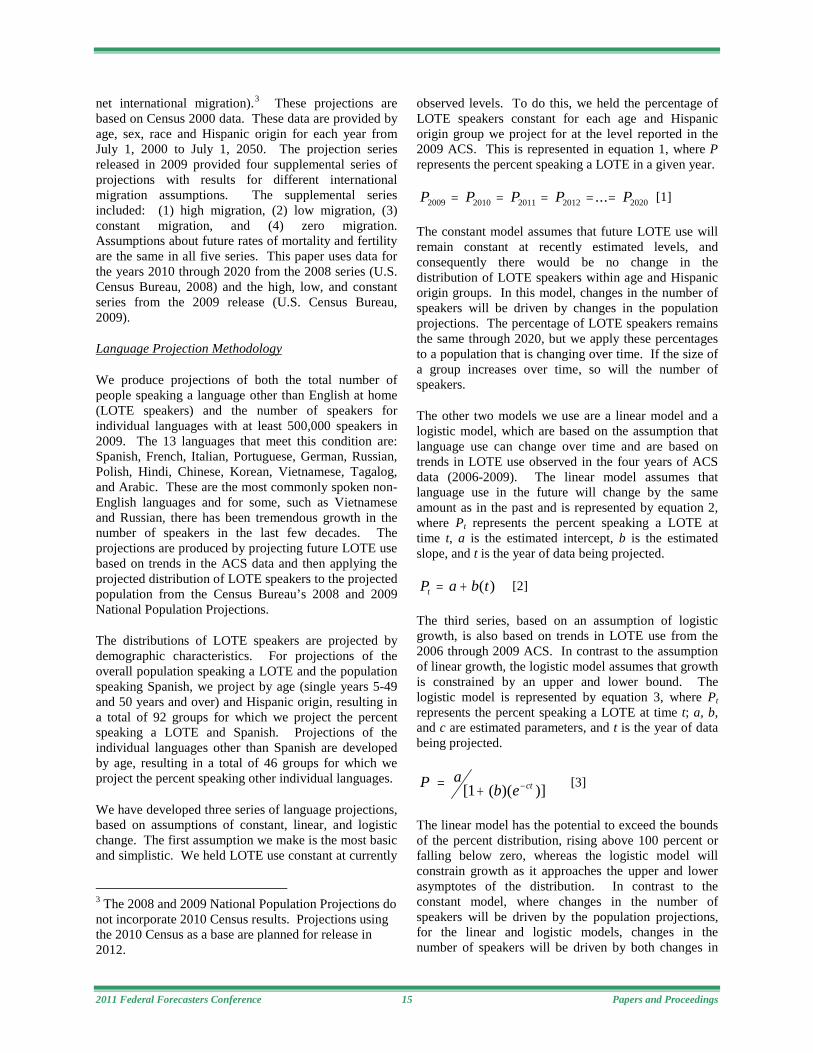
These projections are based on Census 2000 data. These data are provided by age, sex, race and Hispanic origin for each year from July 1, 2000 to July 1, 2050. The projection series released in 2009 provided four supplemental series of projections with results for different international migration assumptions. The supplemental series included: (1) high migration, (2) low migration, (3) constant migration, and (4) zero migration. Assumptions about future rates of mortality and fertility are the same in all five series. This paper uses data for the years 2010 through 2020 from the 2008 series (U.S. Census Bureau, 2008) and the high, low, and constant series from the 2009 release (U.S. Census Bureau, 2009).
We produce projections of both the total number of people speaking a language other than English at home (LOTE speakers) and the number of speakers for individual languages with at least 500,000 speakers in 2009. The 13 languages that meet this condition are: Spanish, French, Italian, Portuguese, German, Russian, Polish, Hindi, Chinese, Korean, Vietnamese, Tagalog, and Arabic. These are the most commonly spoken non-English languages and for some, such as Vietnamese and Russian, there has been tremendous growth in the number of speakers in the last few decades. The projections are produced by projecting future LOTE use based on trends in the ACS data and then applying the projected distribution of LOTE speakers to the projected population from the Census Bureau’s 2008 and 2009 National Population Projections.
The distributions of LOTE speakers are projected by demographic characteristics. For projections of the overall population speaking a LOTE and the population speaking Spanish, we project by age (single years 5-49 and 50 years and over) and Hispanic origin, resulting in a total of 92 groups for which we project the percent speaking a LOTE and Spanish. Projections of the individual languages other than Spanish are developed by age, resulting in a total of 46 groups for which we project the percent speaking other individual languages.
We have developed three series of language projections, based on assumptions of constant, linear, and logistic change. The first assumption we make is the most basic and simplistic. We held LOTE use constant at currently
3 The 2008 and 2009 National Population Projections do not incorporate 2010 Census results. Projections using the 2010 Census as a base are planned for release in 2012.
observed levels. To do this, we held the percentage of LOTE speakers constant for each age and Hispanic origin group we project for at the level reported in the 2009 ACS. This is represented in equation 1, where P represents the percent speaking a LOTE in a given year.
P P P P P2009 2010 2011 2012 2020= = = = =... [1]
The constant model assumes that future LOTE use will remain constant at recently estimated levels, and consequently there would be no change in the distribution of LOTE speakers within age and Hispanic origin groups. In this model, changes in the number of speakers will be driven by changes in the population projections. The percentage of LOTE speakers remains the same through 2020, but we apply these percentages to a population that is changing over time. If the size of a group increases over time, so will the number of speakers.
The other two models we use are a linear model and a logistic model, which are based on the assumption that language use can change over time and are based on trends in LOTE use observed in the four years of ACS data (2006-2009). The linear model assumes that language use in the future will change by the same amount as in the past and is represented by equation 2, where Pt represents the percent speaking a LOTE at time t, a is the estimated intercept, b is the estimated slope, and t is the year of data being projected.
P a b tt = + ( ) [2]
The third series, based on an assumption of logistic growth, is also based on trends in LOTE use from the 2006 through 2009 ACS. In contrast to the assumption of linear growth, the logistic model assumes that growth is constrained by an upper and lower bound. The logistic model is represented by equation 3, where Pt represents the percent speaking a LOTE at time t; a, b, and c are estimated parameters, and t is the year of data being projected.
P ab e ct= + −[ ( )( )]1 [3]
The linear model has the potential to exceed the bounds of the percent distribution, rising above 100 percent or falling below zero, whereas the logistic model will constrain growth as it approaches the upper and lower asymptotes of the distribution. In contrast to the constant model, where changes in the number of speakers will be driven by the population projections, for the linear and logistic models, changes in the number of speakers will be driven by both changes in
2011 Federal Forecasters Conference 16 Papers and Proceedings
the projected percentages of LOTE speakers within each group and by changes in the population projections.
Comparison of Language Projection Models
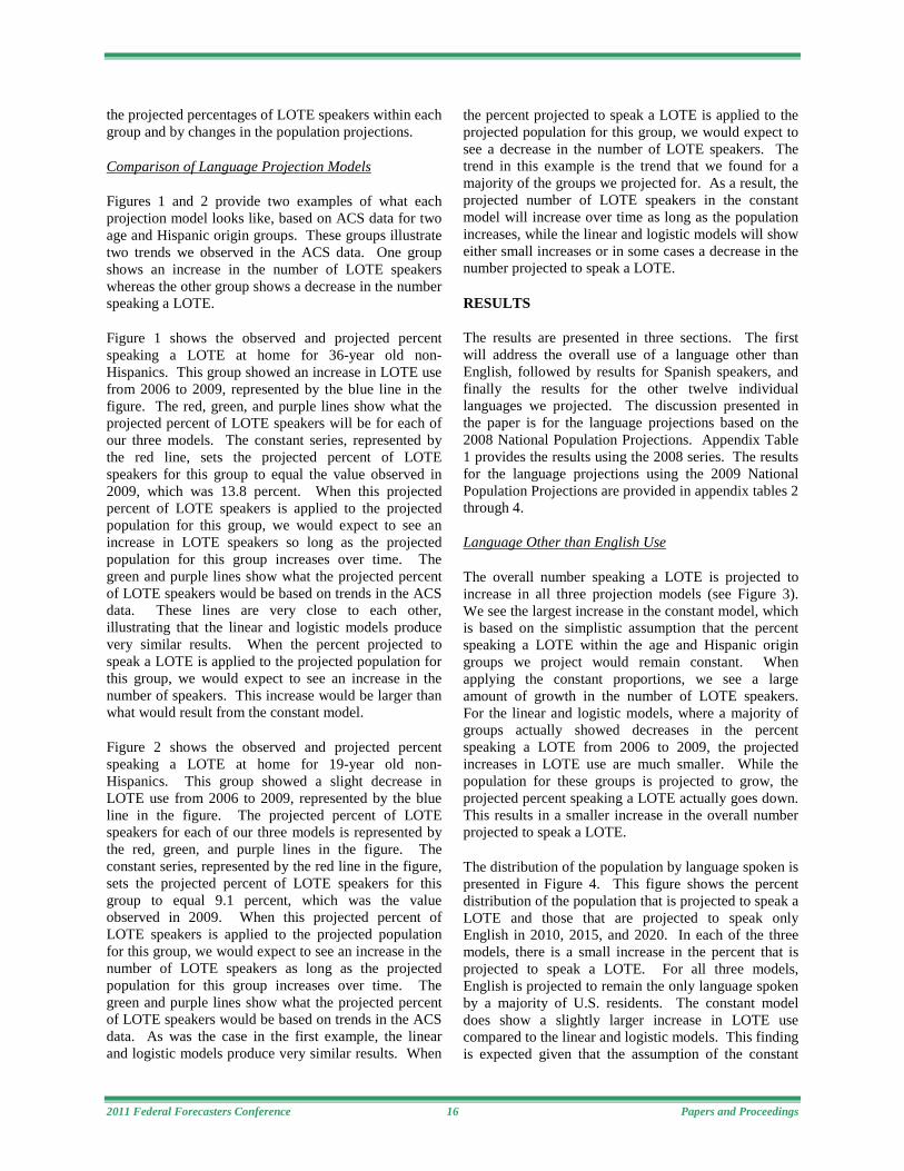
Figures 1 and 2 provide two examples of what each projection model looks like, based on ACS data for two age and Hispanic origin groups. These groups illustrate two trends we observed in the ACS data. One group shows an increase in the number of LOTE speakers whereas the other group shows a decrease in the number speaking a LOTE.
Figure 1 shows the observed and projected percent speaking a LOTE at home for 36-year old non-Hispanics. This group showed an increase in LOTE use from 2006 to 2009, represented by the blue line in the figure. The red, green, and purple lines show what the projected percent of LOTE speakers will be for each of our three models. The constant series, represented by the red line, sets the projected percent of LOTE speakers for this group to equal the value observed in 2009, which was 13.8 percent. When this projected percent of LOTE speakers is applied to the projected population for this group, we would expect to see an increase in LOTE speakers so long as the projected population for this group increases over time. The green and purple lines show what the projected percent of LOTE speakers would be based on trends in the ACS data. These lines are very close to each other, illustrating that the linear and logistic models produce very similar results. When the percent projected to speak a LOTE is applied to the projected population for this group, we would expect to see an increase in the number of speakers. This increase would be larger than what would result from the constant model.
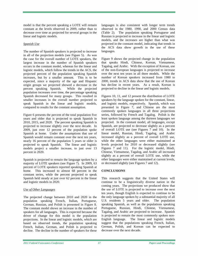
Figure 2 shows the observed and projected percent speaking a LOTE at home for 19-year old non-Hispanics. This group showed a slight decrease in LOTE use from 2006 to 2009, represented by the blue line in the figure. The projected percent of LOTE speakers for each of our three models is represented by the red, green, and purple lines in the figure. The constant series, represented by the red line in the figure, sets the projected percent of LOTE speakers for this group to equal 9.1 percent, which was the value observed in 2009. When this projected percent of LOTE speakers is applied to the projected population for this group, we would expect to see an increase in the number of LOTE speakers as long as the projected population for this group increases over time. The green and purple lines show what the projected percent of LOTE speakers would be based on trends in the ACS data. As was the case in the first example, the linear and logistic models produce very similar results. When
the percent projected to speak a LOTE is applied to the projected population for this group, we would expect to see a decrease in the number of LOTE speakers. The trend in this example is the trend that we found for a majority of the groups we projected for. As a result, the projected number of LOTE speakers in the constant model will increase over time as long as the population increases, while the linear and logistic models will show either small increases or in some cases a decrease in the number projected to speak a LOTE.
RESULTS
The results are presented in three sections. The first will address the overall use of a language other than English, followed by results for Spanish speakers, and finally the results for the other twelve individual languages we projected. The discussion presented in the paper is for the language projections based on the 2008 National Population Projections. Appendix Table 1 provides the results using the 2008 series. The results for the language projections using the 2009 National Population Projections are provided in appendix tables 2 through 4.
Language Other than English Use
The overall number speaking a LOTE is projected to increase in all three projection models (see Figure 3). We see the largest increase in the constant model, which is based on the simplistic assumption that the percent speaking a LOTE within the age and Hispanic origin groups we project would remain constant. When applying the constant proportions, we see a large amount of growth in the number of LOTE speakers. For the linear and logistic models, where a majority of groups actually showed decreases in the percent speaking a LOTE from 2006 to 2009, the projected increases in LOTE use are much smaller. While the population for these groups is projected to grow, the projected percent speaking a LOTE actually goes down. This results in a smaller increase in the overall number projected to speak a LOTE.
The distribution of the population by language spoken is presented in Figure 4. This figure shows the percent distribution of the population that is projected to speak a LOTE and those that are projected to speak only English in 2010, 2015, and 2020. In each of the three models, there is a small increase in the percent that is projected to speak a LOTE. For all three models, English is projected to remain the only language spoken by a majority of U.S. residents. The constant model does show a slightly larger increase in LOTE use compared to the linear and logistic models. This finding is expected given that the assumption of the constant
2011 Federal Forecasters Conference 17 Papers and Proceedings
model is that the percent speaking a LOTE will remain constant at the levels observed in 2009, rather than to decrease over time as projected for several groups in the linear and logistic models.
Spanish Use
The number of Spanish speakers is projected to increase in all of the projection models (see Figure 5). As was the case for the overall number of LOTE speakers, the largest increase in the number of Spanish speakers occurs in the constant model, whereas for the linear and logistic models, which follow the trends in the ACS, the projected percent of the population speaking Spanish increases, but by a smaller amount. This is to be expected, since a majority of the age and Hispanic origin groups we projected showed a decrease in the percent speaking Spanish. While the projected population increases over time, the percentage speaking Spanish decreased for many groups. This resulted in smaller increases in the overall number projected to speak Spanish in the linear and logistic models, compared to results for the constant assumption.
Figure 6 presents the percent of the total population five years and older that is projected to speak Spanish in 2010, 2015, and 2020. The percent speaking Spanish is projected to increase slightly over the next decade. In 2009, just over 12 percent of the population spoke Spanish at home. Under the assumptions that use of Spanish would remain constant over the next ten years, nearly 16 percent of the population 5 years or older is projected to speak Spanish. The linear and logistic models project a smaller increase, to just over 13 percent in 2020.
Spanish is projected to remain the language spoken by a majority of LOTE speakers (see Figure 7). In 2009, 63 percent of LOTE speakers reported speaking Spanish at home. This increased to almost 68 percent in the constant series, while the percent projected to speak Spanish held steady at just over 62 percent in the linear and logistic models in 2020.
Use of Other Languages
The projected change between 2010 and 2020 in the population speaking French, Italian, Portuguese, German, Russian, and Polish is presented in Figure 8. The constant model shows an increase in the number of speakers for all languages. This is expected because the driver of change for this model is the population projections. In the linear and logistic models, which are based on observed trends, the population speaking French, Italian, German, and Polish is projected to decline. The decline in the number of speakers for these
languages is also consistent with longer term trends observed in the 1980, 1990, and 2000 Census data (Table 2). The population speaking Portuguese and Russian is projected to increase in the linear and logistic models, and the increases are higher than what was projected in the constant model, indicating that trends in the ACS data show growth in the use of these languages.
Figure 9 shows the projected change in the population that speaks Hindi, Chinese, Korean, Vietnamese, Tagalog, and Arabic. With the exception of Korean, use of the non-European languages is projected to increase over the next ten years in all three models. While the number of Korean speakers increased from 1980 to 2000, trends in ACS data show that the use of Korean has decline in recent years. As a result, Korean is projected to decline in the linear and logistic models.
Figures 10, 11, and 12 present the distribution of LOTE speakers by the language spoken for the constant, linear, and logistic models, respectively. Spanish, which was presented in Figure 7, and Chinese are the most commonly spoken languages in all three projections series, followed by French and Tagalog. Polish is the least spoken language among the thirteen languages we projected. In the constant model, all languages, except Spanish, are projected to decrease slightly as a percent of overall LOTE use (see Figures 7 and 10). In the linear model, Russian, Hindi, Tagalog, and Arabic increased slightly as a percent of overall LOTE use, while the other languages were either maintained at levels projected for 2010 or decreased slightly (see Figures 7 and 11). For the logistic model, Hindi, Chinese, Vietnamese, Tagalog, and Arabic all increased slightly as a percent of overall LOTE use, while the other languages were either maintained at current levels, or decreased slightly (see Figures 7 and 12).
CONCLUSIONS
This research suggests that the United States will continue to be a linguistically diverse nation in the coming years. The projections we produced show that the use of LOTE is projected to increase over the next ten years, though English is expected to continue to be the only language spoken by a substantial majority of all U.S. residents 5 years and older. The population speaking Spanish, as well as the populations speaking Portuguese, Russian, Hindi, Chinese, Vietnamese, Tagalog, and Arabic are projected to increase. Spanish is projected to remain the most commonly spoken non-English language. The linear and logistic models suggest that the populations speaking French, Italian, German, Polish, and Korean can be expected to decrease over the next decade.

2011 Federal Forecasters Conference 18 Papers and Proceedings
The assumption of constant growth is likely overly simplistic, as it results in an increase in LOTE use for all languages, even those that are shown to decline in Census and in ACS data. The linear and logistic assumptions are perhaps more realistic, following observed trends, and provide results that are very similar. Since the logistic assumption is constrained within upper and lower bounds, and cannot produce projected percentages below zero or above 100, we may consider adopting the logistic model for use in future work.
As we move forward with this research, we plan to add 2010 ACS data to the time series that provides the basis for these projections, extending the time series to five years. We will also use the 2010-Census based population projections when they become available. Increasing the sample size could reduce variation resulting from sampling variability and improve the robustness of our results. In an effort to increase the sample size of the age and Hispanic origin groups we project, we will consider projecting by age groups instead of single years of age or using three-year ACS files instead of single year files to form the basis of the time series.
We will also consider projecting by birth cohorts instead of by age. A cohort approach will entail following cohorts of individuals as they grow older, instead of comparing language use of the population of the same age at different points in time. Studies have shown that language use can shift and change over the life course (Lutz, 2006; Ortman and Stevens, 2008; Portes and Rumbaut, 2001), which supports the adoption of a cohort approach to projecting language use into the future.
We did not project language use by nativity or generational status. Research shows that the use of non-English languages is strongly linked to immigration and is most frequent among first generation residents (Alba et al., 2002; Rumbaut et al., 2006; Stevens, 1992). The Census Bureau’s population projections do not currently separate the population by foreign and native-born status. Should projections by nativity become available, we could further develop our methodology to project by nativity status, which could inform and improve the accuracy of the language projections.
REFERENCES
Alba, Richard, John Logan, Amy Lutz, and Brian Stults. 2002. “Only English by the Third Generation? Loss and Preservation of the Mother Tongue among the Grandchildren of Contemporary Immigrants.” Demography 39(3): 467-484.
Bean, Frank D. and Gillian Stevens. 2005. America’s Newcomers and the Dynamics of Diversity. Russell Sage Foundation: New York.
Chiswick, Barry R. and Paul W. Miller. 2001. “A Model of Destination-Language Acquisition: Application to Male Immigrants in Canada.” Demography 38(3): 391-409.
Cohen-Goldner, Sarit and Zvi Eckstein. 2008. “Labor Mobility of Immigrants: Training, Experience, Language and Opportunities.” International Economic Review 49(3): 837-872.
Espenshade, Thomas J. and Haishan Fu. 1997. “An Analysis of English-Language Proficiency Among U.S. Immigrants.” American Sociological Review 62(2): 288-305.
Hurtado, Aída and Luis A. Vega. 2004. “Shift Happens: Spanish and English Transmission Between Parents and Their Children.” Journal of Social Issues 60:137-155.
Lutz, Amy. 2006. "Spanish Maintenance among English-Speaking Latino Youth: The Role of Individual and Social Characteristics." Social Forces 84(3): 1417-1433.
Mouw, Ted and Yu Xie. 1999. “Bilingualism and the Academic Achievement of First- and Second-Generation Asian Americans: Accommodations With or Without Assimilation.” American Sociological Review 64(2): 232-252.
Ortman, Jennifer M. and Gillian Stevens. 2008. “Shift Happens, But When?: Inter- and Intra-Generational Language Shift among Hispanic Americans.” Presented at the Annual Meetings of the Population Association of America, April 17-19, New Orleans, LA.
Portes, Alejandro and Rubén G. Rumbaut. 2001. Legacies: The Story of the Immigrant Second Generation. Berkeley: University of California Press.
Rumbaut, Rubén G. 1997. “Paradoxes (and Orthodoxies) of Assimilation.” Sociological Perspectives 40:483-511.
Rumbaut, Rubén G., Douglas S. Massey, and Frank D. Bean. 2006. “Linguistic Life Expectancies: Immigrant Language Retention in Southern California.” Population and Development Review 32(3): 447-460.

2011 Federal Forecasters Conference 19 Papers and Proceedings
Shin, Hyon B. and Rosalind Bruno. 2003. “Language Use and English-Speaking Ability: 2000.” U.S. Census Bureau, Washington, D.C.
Stevens, Gillian. 1992. “The Social and Demographic Context of Language Use in the United States.” American Sociological Review 57(2): 171-185.
_____. 1994. “Immigration, Emigration, Language Acquisition, and the English Language Proficiency of Immigrants in the United States.” Pp. 163-185 in Immigration and Ethnicity: The Integration of America's Newest Arrivals, edited by B. Edmonston and J. S. Passel. Washington, D.C.: The Urban Institute Press.
_____. 1999. “A Century of U.S. Censuses and the Language Characteristics of Immigrants.” Demography 36(3): 387-397.
U.S. Census Bureau. 2008. “2008 National Population Projections.” Washington, DC: U.S. Census Bureau. (http://www.census.gov/population/www/projections/2008projections.html).
_____. 2009. “2009 National Population Projections (Supplemental).” Washington, DC: U.S. Census Bureau. (http://www.census.gov/population/www/projections/2009projections.html).

2011 Federal Forecasters Conference 20 Papers and Proceedings
0
2
4
6
8
10
12
14
16
18
20
2006 2007 2008 2009 2010 2011 2012 2013 2014 2015 2016 2017 2018 2019 2020
Observed Constant Linear Logistic
Figure 1. Observed and Projected Percent Speaking a Language Other than English for 36-Year Old Non-Hispanics: 2006-2020
Source: U.S. Census Bureau
Observed Projected
0
2
4
6
8
10
12
14
16
18
20
2006 2007 2008 2009 2010 2011 2012 2013 2014 2015 2016 2017 2018 2019 2020
Observed Constant Linear Logistic
Figure 2. Observed and Projected Percent Speaking a Language Other than English for 19-Year Old Non-Hispanics: 2006-2020
Source: U.S. Census Bureau
Observed Projected
58.6 58.1 58.1
64.962.8 62.4
71.8
67.3 66.3
Constant Linear Logistic
2010 2015 2020
Figure 3. Projections of the Population 5 Years and Older Speaking a Language Other than English at Home in the United States: 2010, 2015, and 2020 (Numbers in millions)
Based on the 2008 National Population ProjectionsSource: U.S. Census Bureau
20.3 21.4 22.5 20.1 20.7 21.1 20.1 20.6 20.8
79.7 78.6 77.5 79.9 79.3 78.9 79.9 79.4 79.2
0
25
50
75
100
2010 2015 2020 2010 2015 2020 2010 2015 2020
Constant Model Linear Model Logistic Model
LOTE Only English
Figure 4. Percent of Population 5 Years and Older Projected to Speak only English or a Language Other than English: 2010 and 2020
Based on the 2008 National Population ProjectionsSource: U.S. Census Bureau
36.8 36.2 36.2
42.5
39.3 39.1
48.7
42.2 41.5
Constant Linear Logistic
2010 2015 2020
Figure 5. Projections of the Population 5 Years and Older Speaking Spanish at Home in the United States: 2010, 2015, and 2020 (Numbers in millions)
Based on the 2008 National Population ProjectionsSource: U.S. Census Bureau
12.7 12.5 12.514.0 13.0 12.915.3
13.3 13.0
0
25
50
75
100
Constant Model Linear Model Logistic Model
2010 2015 2020
Figure 6. Percent of the Population 5 Years and Older Projected to Speak Spanish: 2010, 2015, and 2020
Based on the 2008 National Population ProjectionsSource: U.S. Census Bureau

2011 Federal Forecasters Conference 21 Papers and Proceedings
62.8 62.3 62.365.5
62.6 62.6
67.8
62.7 62.6
0
25
50
75
100
Constant Model Linear Model Logistic Model
2010 2015 2020
Figure 7. Percent of Language Other than English Speakers Projected to Speak Spanish: 2010, 2015, and 2020
Based on the 2008 National Population ProjectionsSource: U.S. Census Bureau
119.6
-152.0
-48.4
55.6
-251.0
-146.2
41.6
141.9
108.8
71.1
-77.5
-112.4
53.7
220.4
126.7
41.7
-189.1
-118.2
Cons
tant
Line
ar
Logi
stic
Cons
tant
Line
ar
Logi
stic
Cons
tant
Line
ar
Logi
stic
Cons
tant
Line
ar
Logi
stic
Cons
tant
Line
ar
Logi
stic
Cons
tant
Line
ar
Logi
stic
French Italian Portuguese German Russian Polish
Figure 8. Projected Change in the Number Speaking a European Language: 2010 to 2020(Numbers in thousands)
Based on the 2008 National Population ProjectionsSource: U.S. Census Bureau
37.3
235.4
173.5147.4
315.1
502.3
60.1
-135.6
-57.4
75.3
182.9
232.0
97.1
317.8297.2
45.6
442.5
246.8
Cons
tant
Line
ar
Logi
stic
Cons
tant
Line
ar
Logi
stic
Cons
tant
Line
ar
Logi
stic
Cons
tant
Line
ar
Logi
stic
Cons
tant
Line
ar
Logi
stic
Cons
tant
Line
ar
Logi
stic
Hindi Chinese Korean Vietnamese Tagalog Arabic
Figure 9. Projected Change in the Number Speaking a Non-European Language: 2010 to 2020(Numbers in thousands)
Based on the 2008 National Population ProjectionsSource: U.S. Census Bureau
0
5
10 2010 2015 2020
Figure 10. Percent Distribution of Language-Other-than-English Speakers by Language Spoken for the Constant Model: 2010, 2015, and 2020
Based on the 2008 National Population ProjectionsSource: U.S. Census Bureau
0
5
10 2010 2015 2020
Figure 11. Percent Distribution of Language-Other-than-English Speakers by Language Spoken for the Linear Model: 2010, 2015, and 2020
Based on the 2008 National Population ProjectionsSource: U.S. Census Bureau
0
5
10 2010 2015 2020
Figure 12. Percent Distribution of Language-Other-than-English Speakers by Language Spoken for the Logistic Model: 2010, 2015, and 2020
Based on the 2008 National Population ProjectionsSource: U.S. Census Bureau

2011 Federal Forecasters Conference 22 Papers and Proceedings
Table 1. Languages Spoken at Home: 1980, 1990, 2000, and 2009
Characteristic 1980 1990 2000 2006 2007 2008 2009
Percentage change
1980-2009
Population 5 Years and older 210,247,455 230,445,777 262,375,152 279,012,712 280,950,438 283,156,079 285,797,349 35.9Spoke only English at home 187,187,415 198,600,798 215,423,557 224,154,288 225,505,953 227,295,534 228,699,523 22.2Spoke a language other than English at home 23,060,040 31,844,979 46,951,595 54,858,424 55,444,485 55,860,545 57,097,826 147.6
Spoke a language other than English at home2 23,060,040 31,844,979 46,951,595 54,858,424 55,444,485 55,860,545 57,097,826 147.6Spanish or Spanish Creole 11,116,194 17,345,064 28,101,052 34,044,945 34,547,077 34,615,394 35,468,501 219.1French (includes Patois, Cajun, Creole) 1,550,751 1,930,404 2,097,206 1,997,618 1,984,824 1,973,531 1,964,556 26.7Italian 1,618,344 1,308,648 1,008,370 828,524 798,801 782,173 753,992 -53.4Portuguese or Portuguese Creole 351,875 430,610 564,630 683,405 687,126 661,120 731,282 107.8German 1,586,593 1,547,987 1,383,442 1,135,999 1,104,354 1,121,465 1,109,216 -30.1Russian 173,226 241,798 706,242 823,210 851,174 860,568 881,723 409.0Polish 820,647 723,483 667,414 640,265 638,059 616,492 593,598 -27.7Hindi1 (NA) (NA) 317,057 504,607 532,911 562,587 560,983 (NA)Chinese 630,806 1,319,462 2,022,143 2,492,871 2,464,572 2,473,968 2,600,150 312.2Korean 266,280 626,478 894,063 1,060,631 1,062,337 1,048,400 1,039,021 290.2Vietnamese 197,588 507,069 1,009,627 1,207,721 1,207,004 1,236,419 1,251,468 533.4Tagalog 474,150 843,251 1,224,241 1,415,599 1,480,429 1,496,208 1,513,734 219.3Arabic 217,529 355,150 614,582 732,519 767,319 780,995 845,396 288.6
NA Not available.
1 Prior to 2000, Hindi and Urdu speakers w ere combined in the same language group (Indic languages). Individual estimates of Hindi speakers are not available for 1980 and 1990.
Sources: U.S. Census Bureau, 1980 and 1990 Census, Census 2000, and 2006-2009 American Community Survey.
2 The total does not match the sum of the 17 languages listed in this table because the total includes other languages that are not listed here. The 13 languages listed in this tables are those language w ith 500,000 or more speakers in 2009.

2011 Federal Forecasters Conference 23 Papers and Proceedings
Very well Well Not well Not at all
Population 5 years and older 285,797,349 (X) (X) (X) (X) (X)Spoke only English at home 228,699,523 (X) (X) (X) (X) (X)Spoke a language other than English at home 57,097,826 100.0 56.9 19.6 15.9 7.5
Spoke a language other than English at home 57,097,826 100.0 56.9 19.6 15.9 7.5
Spanish or Spanish Creole 35,468,501 62.1 54.3 18.0 17.9 9.8
Other Indo-European languages 10,495,295 18.4 67.5 19.6 10.1 2.8French 1,305,503 2.3 79.9 13.9 5.7 0.5French Creole 659,053 1.2 54.2 25.9 15.1 4.8Italian 753,992 1.3 72.6 17.5 8.8 1.0Portuguese 731,282 1.3 58.6 20.8 15.3 5.3German 1,109,216 1.9 83.3 12.6 3.8 0.2Yiddish 148,155 0.3 66.2 19.4 11.0 3.4Other West Germanic languages 271,227 0.5 77.7 18.0 3.7 0.7Scandinavian languages 126,337 0.2 89.0 9.2 1.8 .Greek 325,747 0.6 75.3 15.1 8.7 0.9Russian 881,723 1.5 49.8 27.3 17.2 5.7Polish 593,598 1.0 57.6 25.5 14.0 2.9Serbo-Croatian 269,333 0.5 61.4 21.7 13.6 3.3Other Slavic languages 298,094 0.5 61.5 21.7 13.2 3.6Armenian 242,836 0.4 54.8 22.5 14.7 8.1Persian 396,769 0.7 62.1 21.8 11.3 4.8Gujarathi 341,404 0.6 64.2 20.2 11.8 3.9Hindi 560,983 1.0 78.0 16.0 4.9 1.1Urdu 355,964 0.6 70.3 18.7 8.7 2.2Other Indic languages 668,596 1.2 60.6 23.5 11.1 4.7All other Indo-European languages 455,483 0.8 64.1 23.4 9.3 3.2
Asian and Pacific Island languages 8,698,825 15.2 51.8 25.8 17.1 5.3Chinese 2,600,150 4.6 45.1 26.0 19.5 9.4Japanese 445,471 0.8 55.3 27.5 15.6 1.5Korean 1,039,021 1.8 43.3 28.5 23.6 4.6Mon-Khmer, Cambodian 202,033 0.4 48.4 23.6 21.9 6.1Hmong 193,179 0.3 53.5 24.6 15.2 6.6Thai 152,679 0.3 48.5 32.1 17.0 2.4Laotian 146,297 0.3 50.2 24.5 20.3 5.0Vietnamese 1,251,468 2.2 39.2 27.1 26.2 7.5Other Asian languages 792,756 1.4 68.4 20.8 8.4 2.4Tagalog 1,513,734 2.7 68.5 24.4 6.6 0.5Other Pacific Island languages 371,653 0.7 60.8 25.7 12.3 1.2
Other languages 2,435,205 4.3 69.0 20.1 8.5 2.3Navajo 169,009 0.3 77.3 13.6 6.8 2.3Other Native American languages 196,372 0.3 84.5 11.3 3.7 0.5Hungarian 90,612 0.2 67.4 24.1 8.0 0.5Arabic 845,396 1.5 63.0 22.9 11.3 2.8Hebrew 221,593 0.4 82.1 14.8 2.8 0.2African languages 777,553 1.4 67.7 22.2 7.8 2.2All other languages 125,054 0.2 61.6 17.2 13.9 7.3
X Not applicable.
Sources: U.S. Census Bureau, The 2009 American Community Survey.For more information on ACS see http://w w w .census.gov/acs/w w w /
Number of speakers
Percentage of speakers
of a non-English
language
English-speaking ability
Table A-1. Detailed Languages Spoken at Home by English-Speaking Ability for the Population 5 Years and Older: 2009

2011 Federal Forecasters Conference 24 Papers and Proceedings
2010 2015 2020 2010 2015 2020 2010 2015 2020
Population ages 5 and over 286,998 299,378 311,886 100.0 100.0 100.0 (X) (X) (X)Constant Model
Only English 230,573 238,538 246,736 80.3 79.7 79.1 (X) (X) (X)Language other than English 58,560 64,926 71,805 20.4 21.7 23.0 100.0 100.0 100.0
Spanish 36,780 42,500 48,711 12.8 14.2 15.6 62.8 65.5 67.8French 1,934 1,994 2,054 0.7 0.7 0.7 3.3 3.1 2.9Italian 652 681 707 0.2 0.2 0.2 1.1 1.0 1.0Portuguese 762 782 804 0.3 0.3 0.3 1.3 1.2 1.1German 1,031 1,066 1,102 0.4 0.4 0.4 1.8 1.6 1.5Russian 881 908 934 0.3 0.3 0.3 1.5 1.4 1.3Polish 555 578 597 0.2 0.2 0.2 0.9 0.9 0.8Hindi 601 621 638 0.2 0.2 0.2 1.0 1.0 0.9Chinese 2,623 2,694 2,771 0.9 0.9 0.9 4.5 4.1 3.9Korean 1,051 1,077 1,111 0.4 0.4 0.4 1.8 1.7 1.5Vietnamese 1,300 1,335 1,376 0.5 0.4 0.4 2.2 2.1 1.9Tagalog 1,448 1,495 1,545 0.5 0.5 0.5 2.5 2.3 2.2Arabic 911 932 956 0.3 0.3 0.3 1.6 1.4 1.3
Linear ModelOnly English 231,001 240,692 251,202 80.5 80.4 80.5 (X) (X) (X)Language other than English 58,132 62,772 67,339 20.3 21.0 21.6 100.0 100.0 100.0
Spanish 36,238 39,305 42,229 12.6 13.1 13.5 62.3 62.6 62.7French 1,912 1,846 1,760 0.7 0.6 0.6 3.3 2.9 2.6Italian 625 508 373 0.2 0.2 0.1 1.1 0.8 0.6Portuguese 750 815 891 0.3 0.3 0.3 1.3 1.3 1.3German 1,023 990 945 0.4 0.3 0.3 1.8 1.6 1.4Russian 892 999 1,113 0.3 0.3 0.4 1.5 1.6 1.7Polish 539 452 350 0.2 0.2 0.1 0.9 0.7 0.5Hindi 627 742 862 0.2 0.2 0.3 1.1 1.2 1.3Chinese 2,601 2,758 2,916 0.9 0.9 0.9 4.5 4.4 4.3Korean 1,033 959 898 0.4 0.3 0.3 1.8 1.5 1.3Vietnamese 1,309 1,394 1,492 0.5 0.5 0.5 2.3 2.2 2.2Tagalog 1,474 1,624 1,792 0.5 0.5 0.6 2.5 2.6 2.7Arabic 933 1,147 1,375 0.3 0.4 0.4 1.6 1.8 2.0
Logistic ModelOnly English 231,037 241,055 252,216 80.5 80.5 80.9 (X) (X) (X)Language other than English 58,096 62,409 66,325 20.2 20.8 21.3 100.0 100.0 100.0
Spanish 36,221 39,072 41,525 12.6 13.1 13.3 62.3 62.6 62.6French 1,921 1,896 1,872 0.7 0.6 0.6 3.3 3.0 2.8Italian 629 548 482 0.2 0.2 0.2 1.1 0.9 0.7Portuguese 748 805 857 0.3 0.3 0.3 1.3 1.3 1.3German 1,017 958 904 0.4 0.3 0.3 1.8 1.5 1.4Russian 887 961 1,013 0.3 0.3 0.3 1.5 1.5 1.5Polish 544 480 426 0.2 0.2 0.1 0.9 0.8 0.6Hindi 621 711 794 0.2 0.2 0.3 1.1 1.1 1.2Chinese 2,629 2,873 3,131 0.9 1.0 1.0 4.5 4.6 4.7Korean 1,024 949 966 0.4 0.3 0.3 1.8 1.5 1.5Vietnamese 1,300 1,381 1,532 0.5 0.5 0.5 2.2 2.2 2.3Tagalog 1,475 1,619 1,773 0.5 0.5 0.6 2.5 2.6 2.7Arabic 923 1,065 1,170 0.3 0.4 0.4 1.6 1.7 1.8
Source: U.S. Census Bureau
Table A-2. Projected Population Speaking a Language Other than English at Home: 2010, 2015, and 2020, 2008 National Population Projections
(In thousands)(Percent of population ages 5
and over)
(Percent of population speaking a language other
than English)
X Not applicable.
2011 Federal Forecasters Conference 25 Papers and Proceedings
Comparing Government Forecasts of the United States’ Gross Federal Debt Andrew B. Martinez, The George Washington University
ABSTRACT This paper compares annual one-step-ahead forecasts from the Congressional Budget Office (CBO), the Office of Management and Budget (OMB), and the CBO’s Analysis of the President’s Budget (APB) of the United States’ gross federal debt from 1984 to 2010. While comparisons of these agencies’ forecasts have been done before, they have not focused on the debt. The paper finds that each agency’s forecast lacks something that the other accounts for and an average of the forecasts out performs either agency individually. Keywords: Government Debt, Debt Forecasts, Forecast Evaluation, Forecast Encompassing Acknowledgements: The author would like to thank Neil R. Ericsson, David F. Hendry, and Frederick L. Joutz for their helpful suggestions and comments. In addition the author benefitted from comments at the GWU Brown Bag Seminar on Forecasting, and the Federal Forecasters Conference in Washington DC 2011. I. INTRODUCTION In the aftermath of the recent financial and economic crisis, rapidly increasing government debt around the world has generated increasing worries about economic growth. In 2010, the United States’ total federal government debt outstanding was 92 percent of Gross Domestic Product (GDP), a share that has not been reached since World War II. Recent projections from the Congressional Budget Office (CBO) and the Office of Management and Budget (OMB) both predict government debt will rise above 100 percent of GDP in the near future. These projections have prompted concerns that the United States’ debt burden will become unsustainable and have increased concerns about raising the debt limit. 1
However, upon closer examination there are considerable differences between the available debt forecasts.
The intense focus on the United States’ debt makes it increasingly important to understand how well the debt can be forecast. Furthermore, given the ongoing debate over the debt, it is important to know which forecast
1 For some examples see: Anne Applebaum, “America’s debt spiral resembles Greece’s crisis”, Washington Post, Feb. 17, 2010 and Robert Pozen, “The US Public debt hits its tipping point”, Boston Globe, Feb. 23, 2010.
more closely tracks the trajectory of the debt. This paper aims at answering these questions. Using a time series of the United States’ federal debt, this paper compares how well one-step-ahead debt forecasts from the CBO and the OMB have performed since 1984. The previous literature has extensively compared CBO and OMB forecasts. Overall these studies have mixed results. While some studies find that CBO forecasts are significantly better than OMB forecasts, others find that OMB forecasts are on par with CBO forecasts and even in a few cases the OMB forecasts perform better than the CBO forecasts. These findings tend to vary depending on the time period examined, the variable being forecast and the forecast horizon. This analysis adds to the collection in several ways. First and foremost, it extends forecast comparisons of the CBO and OMB to the federal debt, which has never before been examined. Second, it compares CBO and OMB forecasts against one another individually, with the Analysis of the President’s Budget, and with averages of the agency forecasts. Finally, the analysis makes use of both the root mean square forecasting errors (RMSFE) as well as forecast encompassing to compare the forecasts. This allows for the determination of whether certain forecasts or combination of forecasts can outperform other forecasts. The analysis finds that all of the agency forecasts perform well except during recessions. Furthermore, it shows that a simple average of the agencies’ forecasts performs better than either agency individually. The paper is structured as follows. Section II reviews the previous literature on OMB and CBO forecast comparisons. Section III provides a background to the forecast encompassing test used. Section III describes the data and some initial comparisons of the forecasts. Section IV presents the empirical findings and analysis. Section V concludes. II. LITERATURE REVIEW There is a considerable body of literature that compares CBO and OMB forecasts. These studies can roughly be broken into two different types. The more popular type typically uses the mean square forecasting error (MSFE), the mean absolute error (MAE), or the mean absolute percent error (MAPE) to compare forecasts between the two agencies. The second type uses forecast encompassing tests to compare the forecasts.

2011 Federal Forecasters Conference 26 Papers and Proceedings
Both of these types of studies help to compare forecasts from the two agencies in different ways. Using forecast summary statistics, the first group of studies compares forecasts from the two agencies and come up with a variety of findings. Kamlet, Mowery, and Su (1987) compare one-step and multi-step ahead forecasts from CBO, OMB, their ARIMA model, and the ASA/NBER model for the real growth rate, inflation rate, and unemployment from 1976 to 1984. They find that for short-term forecasts both agencies are “accurate and unbiased” and that neither of the forecasts “outperforms the other in forecasting accuracy”. However, for forecasts extending beyond three years, they find OMB forecasts are “more biased than those of CBO” but are not “less accurate than CBO projections”. Plesko (1988) examines the CBO and OMB forecasts of nominal GNP, current receipts, current outlays, and the deficit from 1974 to 1988 and finds similar results for the short-term forecasts. McNees (1995) compares forecasts from the Federal Reserve Board (FRB), the CBO, the Council of Economic Advisors (CEA)2
, and private forecasters for inflation, GNP, and unemployment from 1976 to 1994. McNees finds similar results for long term forecasts, where the CEA forecasts were more biased than the CBO, FRB and private forecasts. Frendreis and Tatalovich (2000) compare CBO, OMB, and FRB one-step-ahead forecasts of GNP growth, inflation, and unemployment from 1979 to 1997. While all three agencies’ forecasts tend to be close, they find the CBO forecasts to be the best, followed by the FRB, and then the OMB.
The CBO conducts a semi-annual comparison of its forecasts with the OMB and private forecasts. The most recent update is CBO (2010), which compares two-year forecasts and five-year forecasts for output, inflation, three month Treasury rates, long-term interest rates, and wage and salary disbursements from 1980 to 2008. Similar to the previous studies, it finds that the CBO’s two-year forecasts are as accurate as the OMB and private forecasts. The second type of study in the literature uses different types of forecast encompassing tests to compare forecasts and also has somewhat mixed results. Howard (1987) compares the CBO and OMB forecasts of the real GNP growth rate, GNP deflator, consumer price index, unemployment rate, and the three-month Treasury bill rate from 1976 to 1985. By regressing the 2CEA forecasts and OMB forecasts are the same. Thus, studies will either use one or the other to compare against CBO forecasts.
residuals of the OMB forecasts on a constant and the residuals of the CBO forecasts, Howard finds that while errors for both forecasts are strongly correlated, the OMB forecasts are biased. Belongia (1988) compares the Council of Economic Advisors (CEA), the CBO, and private one-step-ahead forecasts of real GNP growth, the GNP deflator, and unemployment from 1976 to 1987. By regressing the actual growth rate of each variable on a constant and different pairs of predicted growth rates, Belongia finds that in general the private forecasts perform better than either the CBO or CEA while neither CBO nor CEA outperform one another. These results suggest that CBO and CEA forecasts may be encompassed by private forecasts of the same variables, but do not encompass one another. Cohen and Follette (2003) compare CBO, OMB and FRB one-step-ahead forecasts of the budget from 1977 to 2003. They regress the actual outcomes on OMB and CBO forecasts over different periods and find that for most samples, CBO forecasts encompass OMB forecasts. Douglas and Krause (2005) also compare CBO, OMB and FRB one-step-ahead forecasts of real and nominal GDP, inflation, unemployment, tax revenues, government outlays, and the budget deficit from 1976 to 2001. They use a variety of encompassing tests, and find that, with the exception of unemployment and tax revenues, the forecasts are not statistically distinguishable from one another. They find that the FRB forecasts perform better than either the CBO or OMB in terms of unemployment, while the CBO forecasts perform worse than either the OMB or the FRB in terms of tax revenues. Corder (2005) examines forecasts of GDP, inflation, unemployment, and interest rates from the Social Security Administration (SSA), the CBO, and the OMB between 1976 and 2003. Using two different tests to check for bias and efficiency, he finds that the CBO forecasts encompass OMB forecasts in terms of GDP, OMB forecasts encompass CBO forecasts in terms of unemployment and inflation, and neither encompasses the other for interest rates. As a result, he concludes that both agencies could improve their forecasts if they incorporated information from the other agency. Overall both types of studies comparing forecasts from the OMB and CBO have mixed results. While some studies find that CBO forecasts are significantly better than OMB forecasts, others find that OMB forecasts are on par with CBO forecasts and even in a few cases the OMB forecasts perform better than the CBO forecasts. For a summary of the previous studies see Table 1.

2011 Federal Forecasters Conference 27 Papers and Proceedings
Both the studies that use standard forecast summary statistics and those that rely on forecast encompassing tests have their limitations. Ericsson (1992) shows that while the MSFE is a necessary condition for ascertaining which forecast is better, it is not sufficient in determining whether one forecast can explain another forecast’s errors (i.e., encompass it). On the other hand, CBO (2010) cautions against using statistical tests with such small sample sizes because, “particular errors can have an unduly large influence on the measures”. Thus, rather than relying on one test or another, this analysis uses a forecast encompassing test along with the root mean squared forecast errors to compare government forecasts of the debt. By doing so, the risk of choosing a less powerful test is spread over a range of tests while allowing for a comparison of the results across tests. III. FORECAST-ENCOMPASSING TESTS The analysis in this paper relies on the root mean squared forecast errors to compare forecasts. It also uses the concept of forecast encompassing developed by Chong and Hendry (1986). They lay out a simple forecast encompassing test to see whether one forecast can better explain the dependent variable than another. Their basic framework is: yt = b0 + b1*xt + b2*zt + error, (1) where b0 is a constant, yt denotes the actual value of the variable being forecast, xt denotes the one-step-ahead forecasts from the first agency and zt denotes the one-step-ahead forecasts from the second agency. Using this approach the null hypothesis tested is {b0=0, b1=1, b2=0} which suggests that the first agency’s forecast provides complete explanation of the dependent variable over the second agency’s forecast and is unbiased. The forecasts can also be rearranged to test whether the second agency’s forecasts “encompass” the first agency’s forecasts. The forecast encompassing test used in this analysis is a very general version of the forecast encompassing framework. Ericsson (1992), Ericsson and Marquez (1993), and Ericsson (1993) provide further variants of this framework. These alternative forecast encompassing tests accommodate different forecast properties and test more specific hypotheses. For a more detailed description of these variants see Martinez (2011). IV. DATA SOURCES AND DESCRIPTIONS This section describes the data used in the analysis and provides some visual comparisons of the forecasts. The primary variable of concern is the log of total gross
federal debt outstanding held by the public and the government in billions of dollars from 1984 to 2010 (LDEBTB). This data is published by the U.S. Department of Treasury’s Financial Management Service and is measured on a fiscal year basis ending on September 30th.3
The federal debt is often overlooked because the change in public debt is usually thought to be equal to the deficit. However, changes in the public debt also include other off budget items that are not included in the deficit; a recent example of this is the Troubled Asset Relief Program (TARP). Furthermore, the federal debt includes debt held by the public, debt held by the government, and agency issued debt. Therefore, it is important to look at the debt since looking only at the deficit would miss other changes to the federal debt. The remaining variables in this analysis span from 1984 to 2010 and come from the annual releases of the CBO’s Budget and Economic Outlook, the OMB’s Budget of the United States Government, and the CBO’s Analysis of the President’s Budget (hereafter APB). These forecasts are typically released at the beginning of the year, usually between January and March, and contain forecasts through to the end of the fiscal year. It is important to note that these forecasts are constrained by different conditions. The CBO forecasts rely on the assumption that current law will be unchanged over the forecast horizon. On the other hand, the OMB and APB forecasts assume that the policy changes proposed in the president’s budget will be implemented. Therefore, these different assumptions may lead to some of the differences between the forecasts. For more information on the forecasts and their release dates see Table 2 in Martinez (2011). The primary variables of interest from the CBO, OMB, and APB are the log levels of the one-step-ahead federal debt forecasts in billions of dollars (LCBODF1, LOMBDF1, and LAPBDF1). Figure 1 plots these forecasts, together with the actual debt to provide an initial view of how they perform. Figure 2 plots the forecast errors, which are generated by subtracting the forecasts from the actual debt. The largest forecast errors for all three forecasts were in 1990, 2001, 2002, 2008, and 2009. These errors make intuitive sense given
3 The face value of the debt is used until 1988 when the Treasury Bulletin started to measure the accrual value of the debt and this practice was also adopted by the CBO and the OMB.
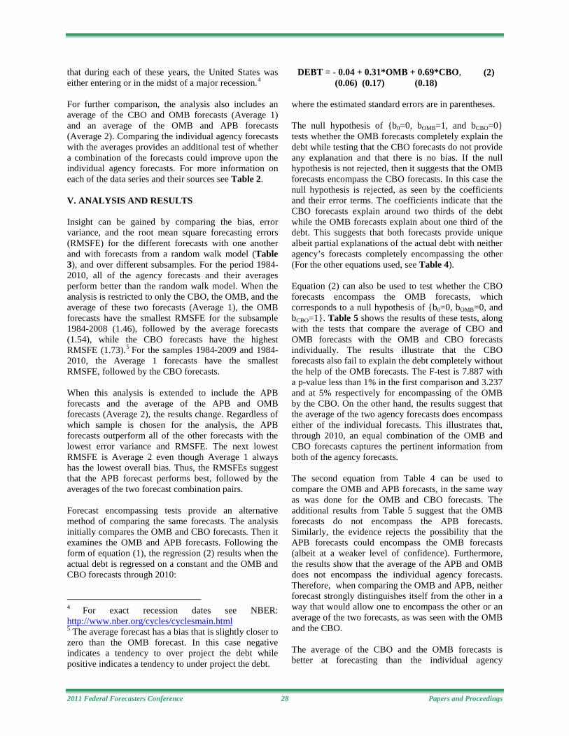
2011 Federal Forecasters Conference 28 Papers and Proceedings
that during each of these years, the United States was either entering or in the midst of a major recession.4
For further comparison, the analysis also includes an average of the CBO and OMB forecasts (Average 1) and an average of the OMB and APB forecasts (Average 2). Comparing the individual agency forecasts with the averages provides an additional test of whether a combination of the forecasts could improve upon the individual agency forecasts. For more information on each of the data series and their sources see Table 2. V. ANALYSIS AND RESULTS Insight can be gained by comparing the bias, error variance, and the root mean square forecasting errors (RMSFE) for the different forecasts with one another and with forecasts from a random walk model (Table 3), and over different subsamples. For the period 1984-2010, all of the agency forecasts and their averages perform better than the random walk model. When the analysis is restricted to only the CBO, the OMB, and the average of these two forecasts (Average 1), the OMB forecasts have the smallest RMSFE for the subsample 1984-2008 (1.46), followed by the average forecasts (1.54), while the CBO forecasts have the highest RMSFE (1.73).5
For the samples 1984-2009 and 1984-2010, the Average 1 forecasts have the smallest RMSFE, followed by the CBO forecasts.
When this analysis is extended to include the APB forecasts and the average of the APB and OMB forecasts (Average 2), the results change. Regardless of which sample is chosen for the analysis, the APB forecasts outperform all of the other forecasts with the lowest error variance and RMSFE. The next lowest RMSFE is Average 2 even though Average 1 always has the lowest overall bias. Thus, the RMSFEs suggest that the APB forecast performs best, followed by the averages of the two forecast combination pairs. Forecast encompassing tests provide an alternative method of comparing the same forecasts. The analysis initially compares the OMB and CBO forecasts. Then it examines the OMB and APB forecasts. Following the form of equation (1), the regression (2) results when the actual debt is regressed on a constant and the OMB and CBO forecasts through 2010: 4 For exact recession dates see NBER: http://www.nber.org/cycles/cyclesmain.html 5 The average forecast has a bias that is slightly closer to zero than the OMB forecast. In this case negative indicates a tendency to over project the debt while positive indicates a tendency to under project the debt.
DEBT = - 0.04 + 0.31*OMB + 0.69*CBO, (2) (0.06) (0.17) (0.18)
where the estimated standard errors are in parentheses. The null hypothesis of {b0=0, bOMB=1, and bCBO=0} tests whether the OMB forecasts completely explain the debt while testing that the CBO forecasts do not provide any explanation and that there is no bias. If the null hypothesis is not rejected, then it suggests that the OMB forecasts encompass the CBO forecasts. In this case the null hypothesis is rejected, as seen by the coefficients and their error terms. The coefficients indicate that the CBO forecasts explain around two thirds of the debt while the OMB forecasts explain about one third of the debt. This suggests that both forecasts provide unique albeit partial explanations of the actual debt with neither agency’s forecasts completely encompassing the other (For the other equations used, see Table 4). Equation (2) can also be used to test whether the CBO forecasts encompass the OMB forecasts, which corresponds to a null hypothesis of {b0=0, bOMB=0, and bCBO=1}. Table 5 shows the results of these tests, along with the tests that compare the average of CBO and OMB forecasts with the OMB and CBO forecasts individually. The results illustrate that the CBO forecasts also fail to explain the debt completely without the help of the OMB forecasts. The F-test is 7.887 with a p-value less than 1% in the first comparison and 3.237 and at 5% respectively for encompassing of the OMB by the CBO. On the other hand, the results suggest that the average of the two agency forecasts does encompass either of the individual forecasts. This illustrates that, through 2010, an equal combination of the OMB and CBO forecasts captures the pertinent information from both of the agency forecasts. The second equation from Table 4 can be used to compare the OMB and APB forecasts, in the same way as was done for the OMB and CBO forecasts. The additional results from Table 5 suggest that the OMB forecasts do not encompass the APB forecasts. Similarly, the evidence rejects the possibility that the APB forecasts could encompass the OMB forecasts (albeit at a weaker level of confidence). Furthermore, the results show that the average of the APB and OMB does not encompass the individual agency forecasts. Therefore, when comparing the OMB and APB, neither forecast strongly distinguishes itself from the other in a way that would allow one to encompass the other or an average of the two forecasts, as was seen with the OMB and the CBO. The average of the CBO and the OMB forecasts is better at forecasting than the individual agency

2011 Federal Forecasters Conference 29 Papers and Proceedings
forecasts, suggesting that the average is more robust to changes in the economy than the individual agency forecasts. This is supported by Clements and Hendry (2004), who show that pooling forecasts can add value when individual forecasting models are differentially mis-specified. Furthermore, Hendry and Mizon (2005) illustrate that there may be a need to pool across forecasting and policy models when there are structural breaks or policy regime shifts. As a result, individual forecasts’ weaknesses can be ameliorated by combining them. Based on the forecast encompassing test, the APB forecasts do not perform significantly better than the OMB forecasts. However, the APB forecasts have the smallest RMSFE. The APB forecasts could also been seen as a quasi forecast combination, in that they are created by the CBO while using the OMB’s assumptions. Therefore, the APB forecasts could also be seen as an average of sorts and its performance could benefit from this combination. There are several possible explanations for why the individual forecasts may be differentially mis-specified. One possible reason stems from the different forecast release dates, which allows the later forecast (typically OMB) to incorporate newer information. Even a small difference in release dates could have a significant impact during a recession or in the midst of large economic and policy changes. Another explanation could be the different assumptions, mentioned above, that the agencies make when producing their forecasts. These assumptions, especially when policies are changing significantly, could lead to large differences in the forecasts. While it is unclear exactly which characteristics of the individual OMB and CBO forecasts lead to their divergence, it is clear that a combination of the forecasts can limit their susceptibility to change. For more information on differences between the OMB and CBO forecasts see Martinez (2011). VI. CONCLUSION This paper compares one-step-ahead debt forecasts from the Congressional Budget Office and the Office of Management and Budget over the past 27 years. While the analysis only looks at the root mean squared forecast errors and one variant of the forecast encompassing test, the results are consistent with the results of other variants of forecast encompassing test, using different samples, and when accounting for potential structural breaks and policy shifts. For these and other results see Martinez (2011).
Overall, the agency forecasts all perform better than a simple benchmark forecast model in terms of the RMSEs. While the CBO forecasts outperform the OMB forecasts through 2010 in terms of the root mean square forecast errors, they fail to completely encompass the information available in the OMB forecasts. Furthermore, the average of the agency forecasts have a lower RMSFE and encompass both the CBO and OMB forecasts individually. While the APB forecasts have the lowest overall RMSFE, there is little evidence to suggest that they can fully explain the debt without the help of the OMB forecasts. In conclusion, while both the Congressional Budget Office and the Office of Management and Budget’s forecasts are relatively successful in forecasting the debt, each agency’s forecast remains incomplete and could benefit from further information that the other agency takes into account. When only one of the agency’s forecasts is used, there is an incomplete and potentially distorted picture of the future levels of the government debt. The evidence is mixed as to whether the Analysis of the President’s Budget can help to improve upon the other two agency forecasts. While the APB forecast is effectively a quasi combination of the two forecasts in that it includes information from both agencies in its forecasts, the evidence suggests that it does not clearly outperform the OMB forecasts. On the other hand, while this analysis did not directly compare the APB forecast with the average of the CBO and OMB forecasts, the root mean square forecast errors indicate that the APB performs best. Even so, the APB’s forecast is released up to several months after the CBO and the OMB forecasts, which reduces its effectiveness for policy making despite the improved information content. Therefore, an average of the two agency forecasts produces the best and most timely forecast of the debt. As a result, it is important that information from both agency forecasts of the debt are taken into consideration to better forecast the future levels of the United States’ gross federal debt.

2011 Federal Forecasters Conference 30 Papers and Proceedings
VII. REFERENCES Applebaum, Anne (2010). “America’s debt spiral resembles Greece’s crisis”. The Washington Post, Feb. 17, 2010. http://www.washingtonpost.com/wp-dyn/content/article/2010/02/16/AR2010021604549.html (accessed November 30, 2010). Belongia, Michael (1988). Are economic forecasts by government agencies biased? Accurate? Federal Reserve Bank of St. Louis Review 70, 15-23. Chong, Yock Y., and David F. Hendry (1986). Econometric Evaluation of Linear Macro-Economic Models. The Review of Economic Studies, 53, no. 4, Econometrics Special Issue (August), 671-690. Clements, Michael P., and David F. Hendry (1993). On the Limitations of Comparing Mean Square Forecast Errors. Journal of Forecasting, 12, no. 8, 617-637. ______ (2004). Pooling of forecasts. Econometrics Journal, 7, 1-31. Cohen, Darrel, and Glenn Follette (2003). Forecasting Exogenous Fiscal Variables in the United States. Federal Reserve Board, Finance and Economics Discussion Series, 59. http://www.federalreserve.gov/pubs/feds/2003/200359/200359abs.html. Corder, Kevin J. (2005). Managing Uncertainty: The Bias and Efficiency of Federal Macroeconomic Forecasts. Journal of Public Administration Research and Theory, 15, no. 1 (January), 55-70. Douglas, James W., and George A. Krause (2005). Institutional Design versus Reputational Effects on Bureaucratic Performance: Evidence from U.S. Government Macroeconomic and Fiscal Projections. Journal of Public Administration Research and Theory, 15, no. 2 (April), 281-306. Engstrom, Erik J., and Samuel Kernell (1999). Serving Competing Principals: The Budget Estimates of OMB and CBO in an Era of Divided Government. Presidential Studies Quarterly, 29, no. 4 (December), 820-829. Ericsson, Neil R. (1992). Parameter Constancy, Mean Square Forecast Errors, and Measuring Forecast Performance: An Exposition, Extensions, and Illustration. Journal of Policy Modeling 14, no. 4, 465-495. Ericsson, Neil R. and Jaime Marquez (1993). Encompassing the Forecasts of U.S. Trade Balance
Models. The Review of Economics and Statistics, 75, no. 1 (February), 19-31. Foster, J. D., and James C. Miller III (2000). The Tyranny of Budget Forecasts. The Journal of Economic Perspectives, 14, no. 3 (Summer), 205-215. Frendreis, John, and Rayond Tatalovich (2000). Accuracy and Bias in Macroeconomic Forecasting by the Administration, the CBO, and the Federal Reserve Board. Polity, 32, no. 4 (Summer), 623-632. Hendry, David F., and Grayham E. Mizon (2001). Forecasting in the Presence of Structural Breaks and Policy Shifts, In, Andrews, Donald W. and Stock, James H. (eds.) Identification and Inference for Econometric Models: Essays in Honor of Thomas Rothenberg
. Cambridge, UK, Cambridge University Press, 480-502.
Howard, James A (1987). Government Economic Projections: A Comparison Between CBO and OMB Forecasts. Public Budgeting & Finance, 7, Issue 3, 14-25. Kamlet, Mark S., David C. Mowery, and Tsai-Tsu Su (1987). Whom Do You Trust? An Analysis of Executive and Congressional Economic Forecasts. Journal of Policy Analysis and Management, 6, no. 3 (Spring), 365-384. Martinez, Andrew B. (2011). Comparing Government Forecasts of the United States’ Gross Federal Debt, GWU RPF Working Paper 2011-2, www.gwu.edu/~forcpgm/2011-002.pdf (accessed February 19, 2011). McNees, Stephen K. (1995). An assessment of the ‘official’ economic forecasts. New England Economic Review (July/August), 13-24. Plesko, George A. (1988). The Accuracy of Government Forecasts and Budget Projections. National Tax Journal, 41, no. 4 (December), 483-501. Pozen, Robert (2010). “The US Public debt hits its tipping point”. The Boston Globe, Feb. 23, 2010. http://www.boston.com/bostonglobe/editorial_opinion/oped/articles/2010/02/23/the_us_public_debt_hits_its_tipping_point/ (accessed November 30, 2010). U.S. Congressional Budget Office (2010). CBO’s Economic Forecasting Record: 2010 Update. www.cbo.gov/doc.cfm?index=11553 (accessed July 10, 2010).
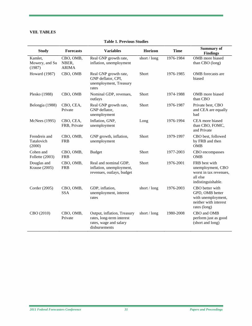
2011 Federal Forecasters Conference 31 Papers and Proceedings
VIII. TABLES
Table 1. Previous Studies
Study Forecasts Variables Horizon Time Summary of Findings
Kamlet, Mowery, and Su (1987)
CBO, OMB, NBER, ARIMA
Real GNP growth rate, inflation, unemployment
short / long 1976-1984 OMB more biased than CBO (long)
Howard (1987) CBO, OMB Real GNP growth rate, GNP deflator, CPI, unemployment, Treasury rates
Short 1976-1985 OMB forecasts are biased
Plesko (1988) CBO, OMB Nominal GDP, revenues, outlays
Short 1974-1988 OMB more biased than CBO
Belongia (1988) CBO, CEA, Private
Real GNP growth rate, GNP deflator, unemployment
Short 1976-1987 Private best, CBO and CEA are equally bad
McNees (1995) CBO, CEA, FRB, Private
Inflation, GNP, unemployment
Long 1976-1994 CEA more biased than CBO, FOMC, and Private
Frendreis and Tatalovich (2000)
CBO, OMB, FRB
GNP growth, inflation, unemployment
Short 1979-1997 CBO best, followed by FRB and then OMB
Cohen and Follette (2003)
CBO, OMB, FRB
Budget Short 1977-2003 CBO encompasses OMB
Douglas and Krause (2005)
CBO, OMB, FRB
Real and nominal GDP, inflation, unemployment, revenues, outlays, budget
Short 1976-2001 FRB best with unemployment, CBO worst in tax revenues, all else indistinguishable.
Corder (2005) CBO, OMB, SSA
GDP, inflation, unemployment, interest rates
short / long 1976-2003 CBO better with GPD, OMB better with unemployment, neither with interest rates (long)
CBO (2010) CBO, OMB, Private
Output, inflation, Treasury rates, long-term interest rates, wage and salary disbursements
short / long 1980-2008 CBO and OMB perform just as good (short and long)

2011 Federal Forecasters Conference 32 Papers and Proceedings
Table 2. Variables
Variable Description Units Periods Sources LDEBTB Annual value of total gross federal debt outstanding (held
by public and intra-governmental holdings) in logs. Billions of Dollars
1984-2010 Financial Management Service (FMS)
LCBODF1 Annual one-step-ahead forecast of Total Gross Federal Debt from the CBO in logs.
Billions of Dollars
1984-2010 Congressional Budget Office
LOMBDF1 Annual one-step-ahead forecast of Total Gross Federal Debt from the OMB in logs.
Billions of Dollars
1984-2010 Office of Management and Budget
LAPBDF1 Annual one-step-ahead forecast of Total Gross Federal Debt from the Analysis of the President’s Budget in logs.
Billions of Dollars
1984-2010 Congressional Budget Office
Table 3. Comparing One-step-ahead Forecasts of the Debt (in %)
Forecast Statistic 1984-2008 1984-2009 1984-2010
CBO Bias 0.18 0.28 0.35
Variance 13.13 13.32 13.31
RMSFE 1.73 1.80 1.80
OMB Bias -0.25 -0.55 -0.60
Variance 12.01 14.43 14.34
RMSFE 1.46 2.15 2.14
APB Bias -0.12 -0.26 -0.29
Variance 11.59 12.16 12.08
RMSFE 1.35 1.50 1.49
Average 1 Bias -0.04 -0.13 -0.13
Variance 12.42 12.61 12.49
RMSFE 1.54 1.60 1.56
Average 2 Bias -0.19 -0.40 -0.45
Variance 11.72 13.18 13.11
RMSFE 1.39 1.78 1.77
RW Model Bias -3.50 -3.08 -2.87
Variance 19.35 20.62 20.77
RMSFE 5.13 5.25 5.18
Notes: 1. A negative bias indicates over predicting while a positive bias indicates under predicting 2. Average 1 is the simple average of the CBO and OMB forecasts. 3. Average 2 is the simple average of the OMB and APB forecasts. 4. RW stands for Random Walk.

2011 Federal Forecasters Conference 33 Papers and Proceedings
Table 4. Comparing Forecast Encompassing Equations: OMB vs. CBO and OMB vs. APB
# Equations (1984-2010)
1 LDEBTB = - 0.0436 + 0.3136 *LOMBDF1 + 0.6916* LCBODF1 (0.0588) (0.1735) (0.1778)
2 LDEBTB = - 0.0813 - 0.9810* LOMBDF1 + 1.9906* LAPBDF1 (0.0492) (0.3409) (0.3446)
Table 5. Forecast-Encompassing Test Statistics for Alternative US Federal Debt Forecasts One-step-ahead (Log levels, 1984-2010)
Encompassing
Forecast Encompassed
Forecast Forecast Encompassing
Test Statistic
OMB CBO 7.887** [0.001] (3,24)
CBO OMB 3.237* [0.040] (3,24)
OMB 0.448
[0.721] (3,24)
CBO 0.448
[0.721] (3,24)
OMB APB 15.293** [0.000] (3,24)
APB OMB 3.215* [0.041] (3,24)
OMB 7.956**
[0.001] (3,24)
APB 7.956**
[0.001] (3,24)
Notes: 1. The three entries within a given block of numbers in the last five columns are: the approximate F statistics for testing the null hypothesis, the tail probability associated with that value of the F statistic (in square brackets), and the degrees of freedom for the F statistic (in parentheses). 2. Asterisks * and ** denote rejection at the 5% and 1% critical values.

2011 Federal Forecasters Conference 34 Papers and Proceedings
IX. FIGURES
Figure 1: Actual Debt, CBO, OMB, and APB one-step-ahead annual debt forecasts, 1984-2010
Figure 2: CBO, OMB, and APB one-step-ahead annual debt forecast errors, 1984-2010
2011 Federal Forecasters Conference 35 Papers and Proceedings
Long Term Medicare Spending Projections Gregory Y. Won, Air Traffic Organization Office of Safety, Federal Aviation Administration
The views in this paper do not represent the views of the Federal Aviation Administration or the Department of Health and Human Services, Centers for Medicare and Medicaid Services.
Abstract
The author develops revised long term forecasts of Medicare Part A expenditures. The revisions correct an inconsistency affecting the official 2010 Medicare Trustees’ projections, and an alternative 2010 projection prepared by the Centers for Medicare and Medicaid Services (CMS), Office of the Actuary. Briefly, the official 2010 Medicare Projections included a price reduction reflecting CMS interpretation of the Patient Protection and Affordable Care Act. However, the price adjustment was already part of the existing projection methodology—essentially, then, the actuaries double counted its effect. The author’s corrections to the Trustees’ methodology increase projected present value Part A 75-year costs by about 36 percent, from $17.1 trillion to $23.3 trillion, increasing the actuarial deficit by 1.62 percentage points. The author concludes with recommendations for improving current Medicare long term projection methods.
I. Introduction
The Statement of Actuarial Opinion in the 2010 Medicare Trustees’ Report to Congress cautioned that: “...the financial projections shown in this report for Medicare do not represent a reasonable expectation for actual program operations in either the short range...or the long range...because of the strong likelihood that the statutory reductions in price updates for most categories of Medicare provider services will not be viable.” Specifically, the official 2010 Medicare projections included an adjustment to reflect annual price updates that will reduce payments for most non-physician services by the growth rate of economy-wide multifactor productivity under a provision of the Patient Protection and Affordable Care Act (PPACA). The Actuarial Opinion concluded that health care providers would not be able to achieve improvements in productivity in line with the annual price adjustments mandated by PPACA, and hence that the official Trustees’ projections “are not reasonable as an indication of actual future costs”.
At least with respect to the long term, however, the 2010 Medicare projections and the Actuarial Opinion were based on a methodological error. Trustees’ projections made prior to 2010 already included an
assumption equivalent to the PPACA productivity adjustment. In fact, the long run parity of medical sector and economy-wide multifactor productivity is explicit in the economic model used to generate the Medicare long term growth pattern. 1
To explain the source of confusion in the 2010 projections this paper: (1) Gives a brief history of U.S. medical spending growth (section II). (2) Describes the Medicare long term projection methodology and explains its underlying productivity growth assumptions (section III). (3) Explains the economic model used to develop Medicare’s long run expenditure growth pattern, and constructs corrected projections of Medicare Part A expenditures (Section IV).
II. Historical U.S. Medical Spending Growth
The practice of medicine, like many other technology-driven fields, has experienced tremendous advances over the last century. Unlike other industries, however, medical technological change has been accompanied by significantly higher costs and an increasing share of total final demand. Figure 1 shows a historical comparison of current dollar National Health Expenditures (NHE), Medicare expenditures and current dollar Gross Domestic Product (GDP) since 1961.2
In 1961 NHE accounted for about 5 percent of GDP, twenty years later it approached 10 percent, and by 2009 it was approximately 17 percent. In fact, medical care is virtually unique among major categories of consumption in that over many decades real medical consumption has grown faster than total consumption,
Between 1960 and 2009, health spending growth has exceeded GDP growth by about 2.5 percent per year, and Medicare growth (since the inception of the program in 1965) has exceeded total economic growth by 4.3 percent.
1 The calculations shown in this paper apply to the 2010 Medicare Trustees’ Report to Congress. However, the basic arguments apply to the 2011 Report, and corrections to the 2011 Medicare projections would be of the same approximate magnitude (in percent terms) as those presented here. 2 1960 is the first year for which an uninterrupted time series of National Health Expenditures is available. Source: Centers for Medicare and Medicaid Services.

2011 Federal Forecasters Conference 36 Papers and Proceedings
even though medical prices have been rising faster than other prices.3
The factors that explain the steadily rising medical share of total final demand can be classified in two general groups: price effects and quantity effects. The former refers to the phenomenon that, since medical prices have historically increased much faster than non-medical prices, the current dollar medical expenditure share has increased (independent of the increase in constant dollar medical care consumption). Figure 2 shows the ratio of medical spending growth (as measured by the Bureau of Labor Statistics medical price index) and All-Urban Consumer Price Index (CPI) growth. Since 1985 medical prices have grown about 2 percent faster per year than the general level of inflation.
Quantity effects refer to factors that have increased the demand for medical services. Broadly, there are three factors that have historically driven the medical spending quantity effect. The first factor is the expansion of health insurance, both as a result of government insurance programs and in the private sector (primarily through employer-provided coverage). The second factor is real income since as income rises consumers tend to increase the consumption of everything, including medical care. The third factor is medical technological innovation.
In principle, medical innovation can have both expenditure-decreasing and expenditure-increasing effects. Expenditure-decreasing innovations reduce treatment costs, e.g., the development of a polio vaccine virtually eliminated the costs associated with treating a life-long crippling disease. Expenditure-increasing innovations raise costs either by introducing therapies for previously untreatable conditions or by providing more expensive alternatives to existing therapies (with presumably greater health benefits), e.g., a new procedure that expands surgical intervention to a larger population of patients.
There is almost universal agreement among health economists that the dominant effect is expenditure-increasing. Estimates of the technology effect suggest that 25-75 percent of the historical increase in medical spending can be ascribed to technological change alone.4
3 See, for example, Borger C, Rutherford TF, Won GY. Projecting Long Term Medical Spending Growth. Journal of Health Economics. 2008 Jan; 27(1): 69–88.
In fact, most experts in the field agree with the
4 See Borger, Rutherford, and Won (2008) for a discussion of this literature. The technology effect is
proposition that the bulk of the increasing medical share of final demand can be ascribed to medical technological innovation.5
III. Medicare Projection Methodology
The Medicare Projections can be divided into short (1 – 10 years into the future), intermediate (11 – 24 years), and long term (25 – 75 years) timeframes. In the short term, projections for Medicare Parts A (hospital insurance), B (medical insurance), and D (prescription drug insurance) are developed separately based on information about various categories of health spending and assumptions about relative medical price inflation and rates of utilization. Therefore, short term forecasted “excess cost growth”--that is, the degree to which per capita cost growth, net demographic effects, exceeds per capita GDP growth--are different for each of Parts A, B, and D. In the intermediate timeframe the separate excess cost growth forecasts are gradually adjusted so that by the 25th year of the projection, they are merged to a single common path that continues into the long run. (Caldis, 2008).
The long run excess cost growth projections have evolved as researchers have acquired a better understanding of the determinants of health spending. Prior to 2000, the Medicare Trustees’ projections assumed that long run average per-beneficiary costs would increase at approximately the same rate as the sources of program funding, and thus at about the same rate as per capita GDP. In defense of actuarial opinion at the time, this assumption, while inconsistent with the history of the medical care industry and the Medicare program, was not patently unreasonable. The Trustees’ projections assume that current laws are fixed; the historical record on the other hand is marked by significant changes in law that resulted in expanded health insurance coverage, including favorable tax treatment for employer-provided health insurance benefits, and the expansion of government medical care programs. sensitive to alternative assumptions about the economics of medical care. 5 This is a long-standing conclusion among experts in the field. In 1996, Victor Fuchs polled 46 leading health economists. Eighty-one percent agreed with the statement: “The primary reason for the increase in the health sector’s share of GDP over the past 30 years is technological change in medicine.” Victor R. Fuchs, “Economics, Values, and Health Care Reform,” American Economic Review, 86:1-24, 1996. See Borger, Rutherford, Won (2008) for a more complete review of the literature on the contribution of technological innovation.

2011 Federal Forecasters Conference 37 Papers and Proceedings
In 2000, the Medicare Trustees convened a Technical Review Panel to study ways to improve the forecast process. A key Panel recommendation was that projected per capita medical spending, net age and gender effects, should grow one percent faster than per capita GDP over the long run time horizon. The growth rule, often referred to as “GDP + 1”, was adopted in 2001 and is the current underlying long term growth assumption.
It is important to understand that GDP + 1 reflects the impact of medical technological innovation. Specifically, the 2000 Panel estimated that one-half of real medical expenditure growth was due to technological innovation. “Attributing 50 percent of the median 4.4-percent growth in real per-capita NHE… to progress in medical technology, the Panel estimates a 2.2-percent growth in real per-capita NHE in the future due to medical technology alone. Subtracting…real per-capita GDP yields a differential of 1 percent.” The Panel was quick to point out, however, that GDP + 1 was at the “lower end of the reasonable range because it assumes that non-technological factors will not continue to contribute to health care expenditure growth.”
In the context of the error in the 2010 Medicare Projections, medical sector price inflation is a particularly important non-technology factor. Long run price inflation, in turn, is related to the relative levels of productivity growth. If medical productivity increases at a slower pace relative to the rest of the economy, then medical care will be more expensive relative to other goods and services, and, as we will demonstrate in simulations below, the medical share of GDP will tend to be higher, ceteris paribus.
Overall, the 2000 Panel concluded that long run productivity growth parity was a reasonable assumption, remarking that “better control of prices by public and private payers, along with properly measured price indices, will result in future increases in health care prices that approximate wage and price growth in the overall economy…[c]urrently, the use of conventional health care price indices gives an overly pessimistic view of productivity gains in medical care.”
To recapitulate, the 2000 Medicare Technical Review panel made the following recommendations (which were later adopted by the Medicare Trustees): (1) The long term medical spending (and, hence, Medicare) growth assumption, net of age and gender effects should be the rate of real per-capita GDP growth plus one percent (“GDP + 1”). This reflected the historical record that suggested that about one-half of historical medical spending growth was due to technological innovation. Multiplying observed real medical spending growth by
50% and then subtracting real GDP growth yielded the one percent differential.6
IV. Alternative Medicare Spending Projections
(2) In the long run, medical sector productivity growth should approach economy-wide productivity growth. Therefore, medical price inflation should be comparable to economy-wide inflation (at least, in the long term future). (3) Other factors, such as the expansion of health insurance coverage, would not continue into the future, and therefore would not be a source of future medical spending growth in excess of GDP growth.
While GDP + 1 was a significant improvement over previous assumptions, it had three weaknesses. First, GDP + 1 itself is inconsistent with historical health-GDP growth patterns. For example, the 2000 Panel noted that the average annualized difference between real National Health Expenditure (NHE) and real GDP growth was 2.7 percent for the post-World War II period. Second, if extrapolated out far enough, the rule implies that virtually the entire economy would consist of health care. Third, the simple growth rule is not linked to explicit theories of consumer behavior and economic production.
The basic problem with GDP + 1 is that it is a mechanical growth rule—there is nothing in the rule to slow future spending growth once the initial trajectory is established. This is illustrated in Figure 3, which is taken from the 2000 Medicare Technical Review Panel report. For example, under “GDP + 1”, the NHE share of GDP is a reasonable 38 percent in 2075. However, under “GDP + 2”, the NHE share is an implausible 80 percent of GDP by 2075.
Borger, Rutherford, Won General Equilibrium Model
In 2006 the Medicare Trustees’ and the Centers for Medicare and Medicaid Services, Office of the Actuary (CMS OACT) adopted a dynamic computable general equilibrium model developed by Borger, Rutherford and Won (BRW, 2008) that partially addressed these problems. (Borger, et al., 2008) The BRW model introduced a formal framework to explain how new technologies affect the demand for medical care. Key was the development of calibration methods that allowed model parameters to be reconciled with
6 As noted in section II, however, the “Quantity Effect”—a combination of factors that affect real consumption including technological innovation and rising income—account for more than one-half of historical medical spending growth under a wide-range of plausible assumptions.

2011 Federal Forecasters Conference 38 Papers and Proceedings
empirical results from previous health economics research. Although technological change is difficult to directly measure in the aggregate, the model equations allow one to infer what the demand effect of technological innovation must have been in order to explain the observed historical pattern of medical spending growth given income and price elasticity estimates derived econometrically and from the literature.
For the purposes of the official Medicare projections the model is constrained in three ways. First, overall economic growth is targeted to the Social Security Trustees’ edlong term real GDP growth projection. Second, medical sector productivity growth is equal to economy-wide productivity growth in the long term. Third, the BRW medical spending projection is computed so that it is consistent with the same Medicare Part A actuarial balance as GDP + 1. Figure 4 shows a BRW model simulation of historical and projected real GDP prepared for this paper.
The simulation results below focus on the effect of our corrections on the financial projections of Medicare Part A. Typically, the status of the program is characterized by the actuarial balance, defined as the difference between average income and cost rates for a given period. In the case of an actuarial deficit, this difference can be interpreted as the number of percentage points by which the payroll tax rate must be raised (or cost rates must be lowered) in order to resolve the program imbalance over the valuation period.
In summary, the long term projection process consists of the following steps:
Step 1: Formulate the long run excess cost growth pattern, by running the BRW model under the three constraints: Social Security Trustees’ GDP projection, medical / non-medical productivity growth parity, and Medicare Part A actuarial balance.
Step 2: Incorporate demographic effects.
Step 3: In the intermediate timeframe gradually transition the short term projections to the long term growth pattern.
Step 4: As discussed above, the 2010 Trustees’ Report included an additional adjustment to account for the multifactor productivity price update under PPACA. Thus, the Medicare Part A growth rate assumptions were determined as described in steps 1 through 3, “minus the full amount of the 10-year average
productivity increase [estimated to average 1.1 percent].”7
At this point, however, it should be clear that the underlying actuarial methodology prior to PPACA already assumed that there would be no long term differential between medical sector and economy-wide productivity growth, and that this assumption was specifically coded into the BRW model. “GDP + 1” is a constant dollar assumption that does not factor in relative medical price inflation.
(Shatto and Clemens, 2010)
Corrected 2010 Medicare Part A Projection
Under the corrected 2010 Part A projection, we assume that PPACA is successful in restraining Medicare cost inflation, and that, in the long term, medical sector productivity growth is equal to that of the rest of the economy. As noted above, this assumption was already explicitly coded into the CMS OACT version of the BRW model prior to 2010, therefore no further adjustment was necessary. The corrected 2010 projection, then, simply removes the 1.1 percent adjustment in the long term timeframe. After correction, Medicare Part A expenditures for 2010 through2084 are estimated to be $23.3 trillion at present value, about 36 percent greater than the 2010 official projection of $17.1 trillion. The corrected actuarial balance, then, is -2.28 percent compared to the official projection of -0.66 percent. Although the corrected figures are significantly higher than the original 2010 Trustees expenditure projections, they are still much lower than the official 2009 forecast.
Corrected CMS OACT Alternative Projection
Based on CMS OACT research, the 2010 Trustees’ Report Actuarial Opinion indicated that it was unlikely that the price adjustments under PPACA could be sustained in the long run. The Opinion pointed readers
7 Prior to PPACA, most Medicare prices were based on input price indices reflecting the costs of factors of production. In principle, then, it would be logical to apply a productivity adjustment to approximate the increase in output prices required by providers to maintain their margins. Under PPACA, the input-based Medicare price update is adjusted to reflect economy wide productivity gains. Based on historical trends, the Medicare Actuaries projection assumes that this adjustment would reduce prices by 1.1 percent per year. The actuaries’ projected adjustment, however, only makes sense if the pre-PPACA projections reflected a productivity-gap between Medicare price inflation and economy-wide inflation of at least 1.1 percent.

2011 Federal Forecasters Conference 39 Papers and Proceedings
to an alternative “Illustrative Scenario” projection, in which the PPACA multifactor productivity adjustments are applied fully through 2019, but then phased out over the 15 years beginning in 2020.
Following the CMS OACT rationale, our corrected alternative scenario posits that productivity growth parity is an implausible long term assumption. Therefore, in our corrected CMS OACT illustrative scenario alternative, we re-run the BRW model and incorporate a 1.1 percent differential between medical sector multifactor productivity growth and productivity growth in the rest of the economy. The productivity differential affects medical expenditures by increasing the relative cost of medical care. (Figure 5 shows the BRW model productivity differential used to generate the results below.) The CMS OACT alternative scenario does not account for this effect, therefore our corrected forecast results in Part A expenditures that are approximately $3 trillion higher than CMS OACT, at present value. Figure 6 compares Medicare Part A costs as a percent of taxable payroll in the official 2010 Trustees’ Report and the CMS OACT illustrative scenario alternative.
Revised 2009 Trustees’ Medicare Projection
If productivity growth parity is an unreasonable assumption, then it follows that Trustees’ projections prior to 2010 are also incorrect. In the third set of simulations, we apply recomputed BRW model results to the 2009 projections, again assuming a 1.1 percent average productivity growth differential. Accounting for lagging medical sector productivity would have increased the Trustees’ 2009 Medicare Part A expenditure projection by approximately 6 percent; $27.3 trillion in our revised forecast versus $25.8 trillion in the official forecast. Our revised 2009 actuarial balance forecast is -4.31 percent, relative to the official 2009 forecast of -3.88 percent. The Table summarizes our results, comparing the original cost and actuarial balance projections to our corrected forecasts.
Conclusions and Future Directions for the Medicare Projections
The errors in the Medicare Trustees’ 2010 projection and the CMS OACT alternative highlight the urgent need to upgrade current Medicare long term forecasting procedures to include: expanded use of economic
modeling, explicit identification of key forecast assumptions, and regular re-evaluation of those assumptions by economic, actuarial and health industry experts. An important benefit of general equilibrium modeling, in particular, is that it enforces consistency from a macroeconomic accounting perspective that is absent in GDP + 1. Formal modeling, in turn, would permit more systematic evaluations of the long term effects of Medicare policy options.
REFERENCES
Borger c, Rutherford TF, Won GY. Projecting Long Term Medical Spending Growth. Journal of Health Economics. 2008 Jan; 27(1): 69–88.
Caldis TG. The Long-Term Projection Assumptions for Medicare and Aggregate National Health Expenditures. Centers for Medicare and Medicaid Services Memorandum. 2008 Mar 25. Available at: https://www.cms.gov/ReportsTrustFunds/downloads/projectionmethodology.pdf.
Shatto JD, Clemens MK. Projected Medicare Expenditures under an Illustrative Scenario with Alternative Payment Updates to Medicare Providers. Centers for Medicare and Medicaid Services Memorandum. 2010 Aug 5. p. 9. Available at: https://www.cms.gov/ReportsTrustFunds/downloads/2010TRAlternativeScenario.pdf.
Technical Review Panel on the Medicare Trustees Reports. Review of Assumptions and Methods of the Medicare Trustees’ Financial Projections. 2000 Dec. Available at: https://www.cms.gov/ReportsTrustFunds/downloads/TechnicalPanelReport2000.pdf.
2004 Technical Review Panel on the Medicare Trustees Report. Review of the Assumptions and Methods of the Medicare Trustees’ Financial Projections. 2004 Dec. Available at: http://www.aspe.hhs.gov/health/medpanel/.
Boards of Trustees of the Federal Hospital Insurance and Federal Supplementary Medical Insurance Trust Funds, 2010 Annual Report of the Boards of Trustees of the Federal Hospital Insurance and Federal Supplementary Medical Insurance Trust Funds. 2010 Aug 5.

2011 Federal Forecasters Conference 40 Papers and Proceedings
Figure 1: Top chart: Ratios of current dollar National Health Expenditure (NHE) and Medicare Growth to current dollar GDP Growth. Bottom chart: NHE share of GDP over time.
Figure 2: Ratio: Medical Price Index growth relative to growth in the Consumer Price Index for all urban consumers. Source: Bureau of Labor Statistics.

2011 Federal Forecasters Conference 41 Papers and Proceedings
Figure 3: NHE share of GDP under different “GDP + X” scenarios.

2011 Federal Forecasters Conference 42 Papers and Proceedings
Figure 4: Historical and Social Security Administration projected real GDP growth compared to a BRW model simulation prepared for this paper. Sources: Historical real GDP growth is from the U.S. Department of Commerce, Bureau of Economic Analysis. The Social Security real GDP projection is from the 2010 Annual Report of Trustees, Federal Old-Age and Survivors Insurance and Federal Disability Insurance Trust Funds, Table V.B2. BRW Model Baseline GDP Simulation reflects the authors’ calculations.
Figure 5: Projected health care price inflation less inflation in the rest of the economy (simulation prepared for this paper). Source: Author’s calculations based on BRW model simulation assuming a 1.1 percent multifactor productivity growth differential between the medical and non-medical sectors.

2011 Federal Forecasters Conference 43 Papers and Proceedings
Figure 6: Projected Medicare Part A costs as a percent of taxable payroll (corrected and uncorrected). Sources: 2010 Medicare Trustees’ report, CMS Office of the Actuary, and authors’ calculations.

2011 Federal Forecasters Conference 44 Papers and Proceedings
Intentionally blank

2011 Federal Forecasters Conference 45 Papers and Proceedings
Consensus and Survey Forecasts
Session Chair: Stephen MacDonald, Economic Research Service, U.S. Department of Agriculture
Evaluating CES/IFO Survey Forecasts of the U.S. Economy Mark Hutson, Fredrick Joutz, and Herman Stekler, The George Washington University
Using the Carlson-Parkin framework and employing the Pesaran-Timmerman Predictive Failure statistic, this paper evaluates several CES/IFO consensus forecasts. Examining issues related to interpreting qualitative survey responses, this paper defines what an “about the same” response implies across different economic variables, the value of agreement across the forecast panel, and how to maximize the signal value provided by the survey. This paper finds that survey respondents provide statistically significant directional forecasts, that forecaster agreement does not aid in determining the magnitude of shifts, and that the survey respondents as a group tend to miss downward turning points.
Measuring Green Economic Activity Ricardo Limes, Bureau of Labor Statistics
There has been much interest lately in the green economy and green jobs both inside and outside of the United States. Several State government-sponsored surveys have been conducted over the past couple of years. While all of the green surveys have measured green activity in the economy, they have used a variety of definitions and measures. The Bureau of Labor Statistics (BLS) is currently collecting and producing information on the occupational employment and wages of green jobs. After researching previous survey efforts BLS settled on a definition of green jobs and green activities. BLS is using two approaches to measuring green jobs: the output approach, which identifies establishments that produce green goods and services, and the process approach, which identifies establishments that use environmentally friendly production processes and practices. Two establishment surveys are underway: a recurring industry survey – the Green Goods and Services Survey as part of the output approach, and as part of the process approach, a special topic survey on green process jobs called the Green Technologies and Practices (GTP) Survey. The GTP Survey will measure jobs in which workers’ duties involve making their establishment’s production processes more environmentally friendly or use fewer natural resources. This presentation will cover previous green survey efforts in the US and abroad, the measures used by BLS for their green surveys, and the development work that BLS has done for the GTP survey.
Forecasters vs. Models: A Horse Race on Monthly Indicator Releases David Payne, U.S. Department of Commerce (Paper following)
The consensus of private forecasters has previously been shown to consistently beat naïve rules in predicting economic indicator releases. However, the race is neck-and-neck when the consensus competes against real time regression models that are presumably similar to what forecasters use. Despite a finding that forecasters’ predictions are biased by over cautiousness, prediction errors are smaller when the consensus is added to the regression models, suggesting a combination approach to forecasting. This result could be interpreted as: the value-added of forecaster judgment, the ability of the consensus to incorporate a wider range of information, or simply as remaining model misspecification.

2011 Federal Forecasters Conference 46 Papers and Proceedings
Intentionally blank

2011 Federal Forecasters Conference 47 Papers and Proceedings
Forecasters vs. Models: A Horse Race on Monthly Indicator Releases By David Payne
Office of the Chief Economist Economics and Statistics Administration,
Department of Commerce The consensus of private forecasters has previously been shown to consistently beat naïve rules in predicting monthly economic indicator releases. However, the race is neck-and-neck when the consensus competes against real time regression models that are presumably similar to what forecasters use. Despite the closeness of the competition, and a finding that forecasters’ predictions are biased and not efficient because they are influenced by overcautiousness, prediction errors are smaller when the consensus is added to the regression models. This result could be interpreted as: the value-added of forecaster judgment, the ability of the consensus to incorporate a wider range of information than models can, or simply as remaining model misspecification. The result can also be interpreted as a view of the consensus as not taking available information into account, because explanatory variables are still significant. This suggests that the best predictions can be made by combining the consensus with a regression model.
Introduction
Economic data releases can move financial markets, to varying degrees. Therefore, many private-sector economists attempt to predict a release’s headline number ahead of time. Surveys collect these predictions and publish a consensus. For monthly data releases, some companies which do this are Dow Jones News, Bloomberg, Thomson Reuters, Market News International, and Money Market Services/Action Economics. Previous studies of these consensus forecasts have examined their rationality using tests of unbiasedness and autocorrelation [Aggarwal, Mohanty, and Song (AMS) 1995; Moersch 2001; Schirm 2003; Campbell and Sharpe 2009; Pandl 2010]. If the consensus is rational, then the difference between the consensus and the data release can be said to accurately reflect the new information that the markets should be reacting to. Non-rational forecasts theoretically ought to be able to be improved using existing information. Section I. below tests the rationality of the consensus forecasts for five economic data releases, and compares the results to these earlier studies. Section II. compares the accuracy of the consensus to various mechanistic models.
I. Tests of Unbiasedness and Efficiency
Forecasts which are rational ought to be both unbiased and efficient. A test of unbiasedness is to run the regression
(1) At = α + βFt + εt
where At is the reported outcome and Ft is the consensus forecast of the data release. If the forecast is unbiased, then it will be distributed randomly around the actual, and so we should see α = 0 and β = 1. If β > 1, this is could be an indication of forecaster over cautiousness. If the forecast is efficient, then εt should be white noise, so that it is not affected by any previous errors. Thus, in the regression
(2) εt = a0 + a1εt-1 + υt
we should see a0 = a1 = 0. The presence of autocorrelation is usually an indication of an omitted variables problem. In this case, a finding of autocorrelation suggests that additional variables need to be added to (1).
This paper uses the Dow Jones News consensus forecasts, and along with Pandl, finds that forecast unbiasedness and efficiency are rejected for most of the data series tested, whereas Schirm and Moersch do not. Table 1 shows that unbiasedness is rejected in time periods when volatility (as measured by the standard deviation) is higher.
There is also some evidence that forecasting is easier and more rational when the autoregressive correlation in the data series is high and positive. For example, for the series in Table 2, the β value climbs when the correlation falls, even though the standard deviations are much lower in the Schirm and Moersch time periods.
II. A Better Test of Forecaster Value-added
Moersch and Pandl test the accuracy of the forecasters’ consensus by comparing their performance against a random walk and a three or six-month moving average, and find that the consensus forecast beats them handily. Although it may be difficult for long run forecasts to beat a random walk, it is doubtful this is the case for the very short run because of the availability of relevant market information. In fact, this paper also finds that forecasters win easily against naïve models when making monthly predictions for five economic data releases. A tougher test for forecasters might therefore
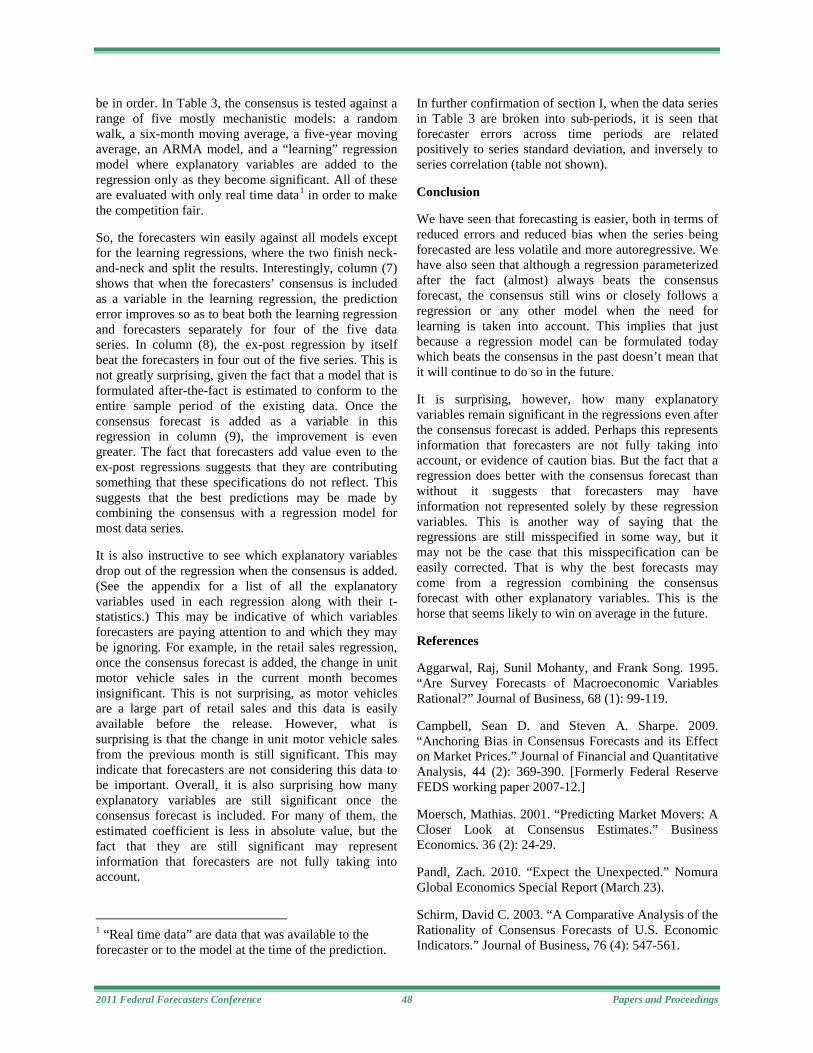
2011 Federal Forecasters Conference 48 Papers and Proceedings
be in order. In Table 3, the consensus is tested against a range of five mostly mechanistic models: a random walk, a six-month moving average, a five-year moving average, an ARMA model, and a “learning” regression model where explanatory variables are added to the regression only as they become significant. All of these are evaluated with only real time data1
So, the forecasters win easily against all models except for the learning regressions, where the two finish neck-and-neck and split the results. Interestingly, column (7) shows that when the forecasters’ consensus is included as a variable in the learning regression, the prediction error improves so as to beat both the learning regression and forecasters separately for four of the five data series. In column (8), the ex-post regression by itself beat the forecasters in four out of the five series. This is not greatly surprising, given the fact that a model that is formulated after-the-fact is estimated to conform to the entire sample period of the existing data. Once the consensus forecast is added as a variable in this regression in column (9), the improvement is even greater. The fact that forecasters add value even to the ex-post regressions suggests that they are contributing something that these specifications do not reflect. This suggests that the best predictions may be made by combining the consensus with a regression model for most data series.
in order to make the competition fair.
It is also instructive to see which explanatory variables drop out of the regression when the consensus is added. (See the appendix for a list of all the explanatory variables used in each regression along with their t-statistics.) This may be indicative of which variables forecasters are paying attention to and which they may be ignoring. For example, in the retail sales regression, once the consensus forecast is added, the change in unit motor vehicle sales in the current month becomes insignificant. This is not surprising, as motor vehicles are a large part of retail sales and this data is easily available before the release. However, what is surprising is that the change in unit motor vehicle sales from the previous month is still significant. This may indicate that forecasters are not considering this data to be important. Overall, it is also surprising how many explanatory variables are still significant once the consensus forecast is included. For many of them, the estimated coefficient is less in absolute value, but the fact that they are still significant may represent information that forecasters are not fully taking into account.
1 “Real time data” are data that was available to the forecaster or to the model at the time of the prediction.
In further confirmation of section I, when the data series in Table 3 are broken into sub-periods, it is seen that forecaster errors across time periods are related positively to series standard deviation, and inversely to series correlation (table not shown).
Conclusion
We have seen that forecasting is easier, both in terms of reduced errors and reduced bias when the series being forecasted are less volatile and more autoregressive. We have also seen that although a regression parameterized after the fact (almost) always beats the consensus forecast, the consensus still wins or closely follows a regression or any other model when the need for learning is taken into account. This implies that just because a regression model can be formulated today which beats the consensus in the past doesn’t mean that it will continue to do so in the future.
It is surprising, however, how many explanatory variables remain significant in the regressions even after the consensus forecast is added. Perhaps this represents information that forecasters are not fully taking into account, or evidence of caution bias. But the fact that a regression does better with the consensus forecast than without it suggests that forecasters may have information not represented solely by these regression variables. This is another way of saying that the regressions are still misspecified in some way, but it may not be the case that this misspecification can be easily corrected. That is why the best forecasts may come from a regression combining the consensus forecast with other explanatory variables. This is the horse that seems likely to win on average in the future.
References
Aggarwal, Raj, Sunil Mohanty, and Frank Song. 1995. “Are Survey Forecasts of Macroeconomic Variables Rational?” Journal of Business, 68 (1): 99-119.
Campbell, Sean D. and Steven A. Sharpe. 2009. “Anchoring Bias in Consensus Forecasts and its Effect on Market Prices.” Journal of Financial and Quantitative Analysis, 44 (2): 369-390. [Formerly Federal Reserve FEDS working paper 2007-12.]
Moersch, Mathias. 2001. “Predicting Market Movers: A Closer Look at Consensus Estimates.” Business Economics. 36 (2): 24-29.
Pandl, Zach. 2010. “Expect the Unexpected.” Nomura Global Economics Special Report (March 23).
Schirm, David C. 2003. “A Comparative Analysis of the Rationality of Consensus Forecasts of U.S. Economic Indicators.” Journal of Business, 76 (4): 547-561.
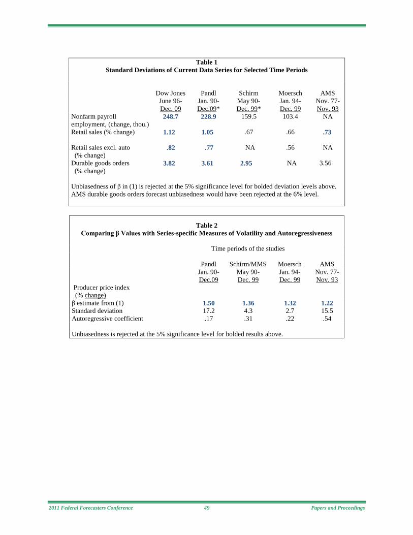
2011 Federal Forecasters Conference 49 Papers and Proceedings
Table 1
Standard Deviations of Current Data Series for Selected Time Periods
Dow Jones
Pandl
Schirm
Moersch
AMS
June 96- Dec. 09
Jan. 90-Dec.09*
May 90- Dec. 99*
Jan. 94- Dec. 99
Nov. 77- Nov. 93
Nonfarm payroll employment, (change, thou.)
248.7 228.9 159.5 103.4 NA
Retail sales (% change)
1.12 1.05 .67 .66 .73
Retail sales excl. auto (% change)
.82 .77 NA .56 NA
Durable goods orders (% change)
3.82 3.61 2.95 NA 3.56
Unbiasedness of β in (1) is rejected at the 5% significance level for bolded deviation levels above. AMS durable goods orders forecast unbiasedness would have been rejected at the 6% level.
Table 2 Comparing β Values with Series-specific Measures of Volatility and Autoregressiveness
Time periods of the studies
Pandl
Schirm/MMS
Moersch
AMS
Jan. 90-Dec.09
May 90- Dec. 99
Jan. 94- Dec. 99
Nov. 77- Nov. 93
Producer price index (% change)
β estimate from (1) 1.50 1.36 1.32 1.22 Standard deviation 17.2 4.3 2.7 15.5 Autoregressive coefficient .17 .31 .22 .54 Unbiasedness is rejected at the 5% significance level for bolded results above.

2011 Federal Forecasters Conference 50 Papers and Proceedings
Table 3
Average Absolute Prediction Error, 2002-09 (1) (2) (3) (4) (5) (6) (7) (8) (9)
Forecasters
Random walk
6-month average
5-year average
ARMA
Learning Regression
Learning Regression with forecasters’ consensus
Ex-post Regression
Ex-post Regression with forecasters’ consensus
Retail sales, %-change
.45 1.17 .84 .80 .75 .50 .41 .44 .37
Retail sales ex auto, %- change
.39 .81 .63 .58 .56 .39 .34 .43 .32
Durable goods orders, %-change
1.97 4.33 2.73 2.50 2.39 1.96 1.91 1.80 1.73
Nonfarm payroll employment, change in thou.
64.7 86.1 93.9 166.6 77.5 61.0 63.8 55.2 54.6
Housing starts, change in thou.
64.7 77.3 84.8 76.9 84.7 67.7 65.9 60.6 58.4
Notes: “Learning” regression is a model where intuitive explanatory variables are only added as they become statistically significant. In the “ex-post” regression, all variables that either start or become significant at some point in the sample period are included in the model specification from the beginning.

2011 Federal Forecasters Conference 51 Papers and Proceedings
Concurrent Sessions II
Risk Forecasting
Session Chair: Grayson Vincent, U.S. Census Bureau, U.S. Department of Commerce
Anomaly Detection Greg Won and Scott Smurthwaite, Federal Aviation Administration
Runway Incursions are one of the Department of Transportation's top safety priorities. The most deadly accident in aviation history (Tenerife Airport, 1977, involving two Boeing 747 aircraft) was a runway incursion accident. The authors will demonstrate a tool that uses statistical techniques to provide predictive warning of runway incursion threat, thus allowing the FAA to proactively manage risk.
Risk Reduction Tools on Dairy Producer Margins: A Production Model with Environmental Effects Roberto Mosheim, Don Blayney and Richard Stillman, Economic Research Service, U.S. Department of Agriculture
Estimates of effects on milk producer margins associated with adoption of risk reduction tools are sought. Producer milk prices have fallen and feed prices have increased recently at the time that both have become more volatile. Exposure to risk is a main driver of decisions of producers wanting to stay in business. These choices can have environmental consequences including changes in land and water use, as well as increases in the number of farms subject to Environmental Protection Agency (EPA) regulation. Time series and simultaneous equations approaches that are part of an ERS dairy forecasting model are used to derive the empirical estimates.
Transition to a Steady State Economy Foster Morrison and Nancy L. Morrison, Turtle Hollow Associates, Inc. (Paper following)
The challenges of the twenty-first century are the exhaustion of nonrenewable resources and the growth of national debt. There are two national policy alternatives: 1) Attempt to ignore the inevitable and keep promoting growth, and 2) Ease the transition to a steady state economy. Option 1 will fail because resources will become more scarce and their prices will rise. Option 2 consists of supporting research on obtaining both materials and energy from limited renewable resources. Catastrophes can be avoided by recognizing problems before they develop into crises.

2011 Federal Forecasters Conference 52 Papers and Proceedings
Intentionally blank

2011 Federal Forecasters Conference 53 Papers and Proceedings
Transition to a Steady State Economy Foster Morrison and Nancy L. Morrison
Turtle Hollow Associates, Inc.
1. What Are the Limits to Growth?
Politicians, economists, business people, and editorial writers are pondering the end of the most recent eco-nomic downturn, the “Great Recession,” and asking when vigorous economic growth will resume. And while it is true that the recession has ended, there has been no strong spurt of growth that brings the GDP back to the level of its long-term trend. See Figures 1 and 2.
Now is a good time to ask whether growth can continue and for how long. The first part is easy. Exponential growth is not sustainable. To determine this one does not need any esoteric mathematics or a state-of-the-art supercomputer. The compound interest formulas (mid-dle-school math) suffice. Constant rate (exponential) growth causes something to double in size in fixed time intervals. Of course, growth rates vary, especially in national economies, so GDPs often double in roughly equal time intervals.
There is no mathematical reason that something cannot double forever. There is no limit to the number of numbers. But there is to the size of tangible objects, the ultimate being collapse into a black hole. Those who lived through the Great Depression will appreciate this analogy.
For 10 doublings, the growth factor is
g(10) = 210 =1024 (1)
So for 20 it is
g(20) = 220 = 1,048,576 (2)
a bit over 1,000,000. There are few things which might grow by a factor of 1000 and almost none by 1,000,000. One exception has been computing power, where the technology used involves making things smaller and smaller, namely electronic components. Moore’s law observes that computing power doubles every two years or so.
Establishing that there are limits to growth, whether of economic activity, population, or anything else is trivial. On the other hand, coming up with numerical estimates of what they are is difficult to do with any precision.
For one thing, there are tradeoffs. One country may choose to have a small population with a high standard of living. Another, a large population living in poverty. National policy almost everywhere seems to be an ex-ponentially expanding population and an economy ex-panding exponentially at a faster rate than the popula-tion, so that the level of consumption may rise. The best way to categorize this is as a belief that “you can have your cake and eat it too.”
The Rev. Thomas Robert Malthus, FRS (1766–1834), was among the first to come to the conclusion that population could not keep growing and that economic production also was limited. He has often been derided for this basic comprehension of reality. While he attributed it to divine plan, it follows from a little basic math and science.
The rapid technological progress of the nineteenth and twentieth centuries obscured the issue of limits, but set into motion processes that would make the end of growth happen sooner and be potentially much more dangerous. Resources, both renewable and nonrenewable, have been consumed with increasing rapidity (Hardin, 1968). In many cases the capacity to produce renewable resources is being diminished.
The then new technology of large, mainframe computers was used to study economic growth in the 1960s. Large-scale dynamical models were constructed using ODEs (ordinary differential equations) solved by numerical means, since that was the only way possible. This work was part of a larger effort called System Dynamics (Forrester, 1961; Randers, 1980). A serious challenge is that even small systems of nonlinear ODEs can have extremely unstable solutions, a phenomenon known as chaos (Gleick, 1987; Morrison, 2008).
These studies were sponsored by a think tank called the Club of Rome. The effort is well summarized thusly:
The originality of their approach soon became clear. In 1972 the campaigning of this growing group of like-minded individuals gained a new worldwide reputation with the first report to the Club of Rome: "The Limits to Growth", commissioned by the Club from a group of systems scientists at the Massachusetts Institute of Technology. The Report explored a number of scenarios
2011 Federal Forecasters Conference 54 Papers and Proceedings
and stressed the choices open to society to reconcile sus-tainable progress within environmental constraints.
(http://www.clubofrome.org/eng/about/4/)
The work continued after this report to the Club of Rome and the results are reported by Meadows, et al., (2004).
A newer and simpler methodology has been developed by the Global Footprint Network based in Oakland, CA. It is basically an accounting methodology that evaluates what resources are available and how much of them are being consumed (Wackernagel, et al., 2002). The latest estimate, for the year 2007, is 150%.
(http://www.footprintnetwork.org/press/lpr2010_Factsheet.pdf)
2. The Known History of US Growth
Some estimates of GDP date to 1860, but regular annual ones are available only after 1889 (U.S. Bureau of Eco-nomic Analysis, 1973). Ones for 1929 through 2010 are available on the Bureau’s website (http://www.bea.gov/index.htm). There are annual values for all these years and quarterly ones starting with 1947.
The data for the years before 1929 are GNP, not GDP, and they were given in 1929 and 1958 dollars, not “chained” 2005 dollars. These data were adjusted by a log-linear regression to fit the 1929 and subsequent GDP data in 2005 dollars. The regression formulas were then extrapolated back to 1889 so that the pre-1929 data were converted to GDP in “chained” 2005 dollars. The results were then averaged, with three data sets covering the period 1909–1928 and two for 1889–1908. The results are given in Table 1.
The US GDP graph in Figure 1 includes a trend model derived from a 20-point ramp filter (Morrison and Morrison, 1997) applied to the logarithms of the data. Figure 2 shows a trend model generated by fitting a second degree polynomial to the logarithms of the data. A back extrapolation from 1889 was done so as not to lose the first 19 years. The data show that the growth factor for GDP was
g(1889, 2010) = 13248.2/178.2
(3)
= 74.34
The average growth rate was 3.63%/year, which equates to a doubling time of about 19.5 years. So the US economy doubled more than 6 times in the period of 121 years, 1889–2010. Is it possible that it will do the same by the year 2131?
3. A Simplified “System Dynamics” Model
The System Dynamics models worked rather well, con-sidering the fact that nonlinear dynamic systems can be chaotic and virtually unpredictable, like the weather and the long-term consequences of global warming.
However, once one realizes that exponential growth is not sustainable and, hence, not an issue, it is possible to begin with a very simple model. A good way to start is by aggregating all resources into the categories of
a. Renewable b. Nonrenewable c. Nonrenewable, but partially recycled
Fresh water is a renewable resource, but one that is be-coming scarce in many areas due to increased demand. The supply is being diminished by pollution, with the extraction of shale oil and gas being a new and poten-tially devastating threat.
Fossil fuels are nonrenewable, unlike wood or solar power. Uranium and other fuels for nuclear reactors are nonrenewable, but can be created with breeder reactors, a technology adopted by France. Nuclear waste is a major problem for the USA and parts of the former USSR, but it could be reprocessed.
Most metals can be recycled and many now are, even that most common of all, iron and its alloy called steel. Many plastics are being recycled, with a large part of the motivation being that landfills are overflowing with yesterday’s trash.
The simplified model assumes a fixed amount of non-renewables and a fixed rate of recycling for some part of them. Renewables are replenished at a constant rate, which may be a bit optimistic, considering the growing threats to water resources.
The economic model consists of a difference equation that attempts to grow exponentially by consuming more and more resources. A difference equation, whether linear or nonlinear, is very easy to solve with an Excel spreadsheet. The level of accuracy of predictions that might be expected from any sort of model of this type and scope does not justify the complexity of differential

2011 Federal Forecasters Conference 55 Papers and Proceedings
equations. Forecasting methodologies use difference equations almost universally, with the basic dynamical model being a noise-driven linear system. The caveat is that the linear system must have no eigenvalues z with a modulus greater than or equal to 1, i.e.,
║z║ < 1 (4)
This assures that the linear system decays exponentially, perhaps with sinusoidal swings, rather than growing exponentially (Morrison, 2008, pp. 175–210).
Figure 3 shows a graph of a projection of US GDP as nonrenewable resources are exhausted and the con-sumption of renewable ones is saturated. Needless to say, this is a highly simplified model, though it may be as accurate a forecast as can be made. In reality, not all nonrenewables will be exhausted at the same time and not all renewables will be saturated simultaneously. Substitution of one resource for another will certainly occur, as it does now when commodity prices vary.
The model does not contain components for the business cycle, which certainly will not go away. However, the business cycle cannot be forecast very well for even one of its variable periods.
The equations could be supplemented by terms for the business cycle and the complex interactions of markets, governments, and consumers, but these would be in the category of emulations, not forecasts. What this means is that the qualitative behavior might be captured, but that the oscillations in the projections will not likely correspond with what will happen. The amplitudes might be good approximations, but the phases would be a lost cause. A property of complex dynamic systems that exist in the real world, whether that of nature or of human actions or the interactions between the two, is that they exhibit some sort of global stability, but are almost chaotic on the local scale.
For example, the weather cannot be forecast very well in most locations, but the climate has been rather stable over periods of years and even decades. Life on Earth has survived for billions of years. Determining whether global warming could destroy this overall stability is a challenge for science and addressing the possibility is an even bigger challenge for governments, industries, other institutions, and the various peoples of the world.
4. What Is the Business Cycle Telling Us Now?
Our phase plane model of the business cycle was indi-cating that a recession might well begin in 2007 or 2008
and this indeed did come to pass. What we did not an-ticipate was the scope or depth of the contraction. While it is true that the growth of subprime mortgages and the securitization of these and other forms of high-risk debt as high-grade securities was being reported in the financial press, nobody seemed aware of the scale of the risks. Eventually everybody found out the hard way.
The methodology of the business cycle model is pre-sented in detail in Morrison and Morrison (1997, 2001, 2002, 2006).
Our most recent plots of the business cycle model indi-cate that a recovery is occurring, though GDP growth is modest and not spiking up to return it to the level of the long-term trend. See Figures 1 and 2. There is no indi-cation that resource shortages caused the “Great Reces-sion,” even though the consumption of renewables may now exceed the sustainable supply by a factor of 150%. However, commodity prices are rising, blamed by some economists on the increasing demand from developing nations (Evans, 2011).
The one event that might well trigger a sudden halt to economic growth is the decline of petroleum production. The giant Ghawar field in Saudi Arabia is nearing the end of its useful life and the new fields being opened there will probably not match its capacity (Chazan, 2008; Day, et al., 2009; Hall and Day, 2009).
Rising prices of commodities may be caused by cur-rency depreciation (inflation) as well as declining sup-plies. The Federal Reserve’s target for inflation is 2%/year, which is small enough that it does not trigger defensive action by either the public or businesses, such as hoarding gold. The rise of gold to the $1400/Troy ounce level has been due to anxieties over a number of things. Few people, not even economists or corporate CEOs, will do the math and observe that this mild infla-tion rate cuts the buying power of the dollar by 50% every 35 years and by 75% in 70 years. The question remains whether we are now seeing a flight from the dollar and, perhaps, from all currencies.
5. The Race between Climate Change and Resource Depletion
The debate about climate change and its possible con-sequences has taken on an ideological dimension. While it is true that everything in science is probabilistic (except perhaps some parts of mathematics) rather than absolute truth, skepticism is always in order. However, the evidence that global warming could have drastic or even catastrophic results is strong. But the evidence that

2011 Federal Forecasters Conference 56 Papers and Proceedings
resource depletion will terminate economic growth is even stronger. So, will economic stagnation arrest climate change?
Not necessarily. As the supply of petroleum declines, the use of coal and natural gas will likely increase to make up for some of the oil. Natural gas and petroleum derived from shale and other nonconventional sources may cause severe environmental damage, including the destruction of fresh water resources.
The basic problem is that neither governments nor in-dustries are prepared for the inevitable. The result may be that either populations or economic activities will overshoot what is sustainable, and perhaps both.
Rare earth metals are already in short supply. These exotic elements, with atomic numbers ranging from 57 (La – Lanthanum) to 71 (Lu – Lutetium) were once scientific curiosities, but they have found many critical uses in modern industry (Hodgman, 1955). China con-trols much of the supply and is trying to retain these metals for its own industries.
Not all nonrenewable resources will be exhausted si-multaneously, of course. Some things can be substituted for others, but only up to a point. Various technologies will have to be abandoned and, to the extent possible, replaced by others. In some cases it may be possible to replace rare metals with organic molecules. Science has its job cut out for it.
6. The Transition to a Steady State Economy
There will be a time lag between the end of the possi-bility for growth and the acceptance of this inevitability. The culture of endless growth and increasing prosperity has spread from what is called “the West,” and espe-cially the USA, to being a global phenomenon. The nations of Asia, with the singular exception of Japan, have been slow to embrace the promises of endless technological progress and the resulting universal pros-perity. But now they have joined in a process that is coming to an end.
The first part of the twenty-first century will be a classic example of “generals fighting the last war over again.” Except that the leaders will be economists, industrialists, and politicians all around the world. The “war” will be one of economic competition and, of course, this may produce actual warfare as it has so often in the past. Some of these wars may already be underway.
Eventually the world’s leaders will conclude that the trade wars and military operations are not solving the problems, but making them worse. The solution is to develop new technologies based on renewable resources and new economies not dependent on endless growth.
7. Smoothing the Transition
A critical role for government in easing the transition to a steady state economy is supporting appropriate re-search. This has been underway for a number of years, but not much has been accomplished. For example, it is not clear whether the ethanol mixed into gasoline uses for its production more or less petroleum than is saved.
The problem of where and how to store nuclear waste is still unresolved, despite the fact that nuclear power might ease the transition away from fossil fuels.
Numerous social problems will arise; some are already here. Addressing these will be difficult and controver-sial. After all, everybody can agree that getting energy from nonpolluting sources benefits everybody. Efforts to stabilize populations, however, will be an almost im-possible challenge due to religions, ethical issues, ide-ologies, ethnic rivalries, and many other factors.
Governmental finances are a major problem already, with nations around the world spending much more than can be collected in tax revenues. More sovereign de-faults will occur as others follow in the steps of Argen-tina. The US dollar will no longer be the global reserve currency and it is unlikely that anything will replace it. Trade will be done with currency swaps, a practice now being used by China, or barter, that was much used in the former Warsaw Pact bloc (of Soviet Satellites). Gold certificates may enjoy a revival, but these will be issued only by private banks or other financial institu-tions that are strictly regulated. President Nixon ended the era of any national currency being a reliable store of value when he closed the gold window in 1971.
8. Conclusions
The age of economic and population growth is coming to an end. Economic and political ideologies must yield to the laws of physics.
Nations and even regions will face a tradeoff of popula-tion size vs. standard of living. This was less apparent as recently as the 1960s (and still is not acknowledged by most people), in part because wars and disease kept populations in check.

2011 Federal Forecasters Conference 57 Papers and Proceedings
Now there are more humane ways to control population size, but numerous cultures reject some or even all of them. The adaptation to a steady state economy will be more difficult for some nations than others.
9. References
Chazan, G., “Fading Oil-Field Production Threatens Supply, IEA Says,” The Wall Street Journal, p. A8, November 13, 2008. To keep up-to-date on peak oil, go to the ASPO website: http://www.peakoil.net/.
Day, J.W., Jr., et al., “Ecology in Times of Scarcity,” BioScience 59: 4, 321-331, April 2009.
Evans, K., “Ahead of the Tape: A Standard-of-Living Shock Is the Danger,” The Wall Street Journal, p. C1, Feb. 17, 2011.
Forrester, J.W., Industrial Dynamics, The M.I.T. Press, Cambridge, MA, 1961.
Gleick, J., Chaos: Making a New Science, Viking Pen-guin, New York, 1987.
Hall, C.A.S. and J.W. Day, Jr., “Revisiting the Limits to Growth After Peak Oil,” American Scientist 97: 230-237, May-June 2009.
Hardin, G., “The Tragedy of the Commons,” Science, 16, 1243- 8, Dec. 13, 1968.
Hodgman, C.D., editor, Handbook of Physics and Chemistry, Thirty-seventh Edition, Chemical Rubber Publishing Company, Cleveland, Ohio, 1955.
Meadows, D., D. Meadows, and J. Randers, Limits to Growth: The 30-Year Update, Chelsea Green Publish-ers, White River, VT, 2004 (Paperback).
Morrison, F., The Art of Modeling Dynamic Systems: Forecasting for Chaos, Randomness, and Determinism, Dover Publications, Mineola, NY, 2008.
Morrison, F. and N.L. Morrison, A phase plane model of the business cycle, The 8th Federal Forecasters Conf - 1996 & The 7th Federal Forecasters Conf. - 1994: Combined Papers & Proceedings, US Dept. of Education, NCES 97-341, pp. 93-112, Debra E. Gerald, editor, Washington, DC, 1997. Available in PDF format at http://www1.va.gov/vhareorg/ffc/ ffc.htm#PandP.
Morrison, F. and N.L. Morrison, An improved phase plane model of the business cycle, The 11th Federal Forecasters Conf. - 2000, US Dept. of Education, NCES 2001-036, pp. 183-191, Debra E. Gerald, editor, Washington, DC, 2001. See above for PDF copies.
Morrison, F. and N.L. Morrison, Forecasting the busi-ness cycle with polar coördinates, The 12th Federal Forecasters Conf. - 2002, pp. 185-191, Debra E. Ger-ald, editor, Washington, DC, 2002. See above for PDF copies.
Morrison, F. and N.L. Morrison, The Recessions of 1990 and 2007(?), The 15th Federal Forecasters Conf. - 2006, pp. 87-97, Jeffrey Busse, et al., editors, 2006. See above for PDF copies.
Randers, J., Elements of the System Dynamics Method, The M.I.T. Press, Cambridge, MA, 1980.
U.S. Bureau of Economic Analysis, Long Term Growth, 1860-1970, Washington, DC, 1973.
Wackernagel, M., et al., Tracking the ecological over-shoot of the human economy, PNAS 99: 14, 9266-9271, 2002 July 9. For the latest on this research visit the website of the Global Footprint Network: http://www.footprintnetwork.org/en/index.php/GFN/

2011 Federal Forecasters Conference 58 Papers and Proceedings
GDPTREND
Year1880 1900 1920 1940 1960 1980 2000 2020
0
2500
5000
7500
10000
12500
15000
Figure 1. US GDP in Billion Chained 2005$ + 20 Point Ramp log Trend
GDPTREND
Year1880 1900 1920 1940 1960 1980 2000 2020
0
2500
5000
7500
10000
12500
15000
Figure 2. US GDP in Billion Chained 2005$ + Quadratic log Trend

2011 Federal Forecasters Conference 59 Papers and Proceedings
Year GDP 2005$ Trend Year GDP 2005$ Trend Year GDP 2005$ Trend 1889 178.2 178.2 1903 362.9 352.6 1917 600.9 632.7 1890 191.2 187.9 1904 371.1 370.5 1918 656.9 653.2 1891 201.0 198.1 1905 397.4 390.8 1919 665.1 673.0 1892 215.8 209.7 1906 428.4 414.1 1920 659.9 687.4 1893 214.4 219.5 1907 443.7 437.4 1921 631.3 695.2 1894 214.5 227.7 1908 433.6 455.7 1922 695.6 711.9 1895 232.4 237.8 1909 475.9 478.9 1923 791.6 742.9 1896 235.1 246.8 1910 489.0 502.3 1924 810.4 771.7 1897 255.6 258.0 1911 510.1 526.5 1925 853.4 805.8 1898 265.9 269.3 1912 533.3 553.1 1926 913.9 849.4 1899 290.2 283.3 1913 548.1 576.1 1927 926.0 891.0 1900 303.6 297.8 1914 534.6 589.4 1928 942.6 925.7 1901 333.8 315.8 1915 545.9 602.2 1929 977.0 966.6 1902 345.5 333.7 1916 592.7 618.0 1930 892.8 984.9
Table 1. US GDP and trend, 1889–1930. The data for 1889–1928 were converted from GNP data in 1929 and 1958 dollars using log-linear regressions and extrapolating back from 1929. The trend is the same as used in Figure 1, the exponenetial function of a 20-point ramp filter applied to the logarithms of the data. GDP data for 1929–2010 are available from the U.S. Bureau of Economic Analysis (http://www.bea.gov/index.htm). The values for 1929 and 1930, as well as the corresponding trend, are included to facilitate comparisons.
Calendar Years1880 1930 1980 2030 2080 2130 2180 2230 2280
USA
GD
P in
Bill
ions
of C
hain
ed 2
005
Dol
lars
0
5000
10000
15000
20000
25000
Model of USA GDP Trend Affected by Depletion of Resources
Model GDP
Actual GDP
Figure 3. A simplified dynamical model of transition to a steady state economy. Of course, the actual transition will almost certainly be much more complex, but any attempt to forecast to that level of precision would be futile.

2011 Federal Forecasters Conference 60 Papers and Proceedings
0°
90°
180°
270°
01/00
01/01
01/02
01/03
01/04
01/0501/06
01/07
01/08
01/09
EXPANSION
RECESSION
B
B
EOfficial endprevious recession
Official beginninglast recession
Official beginningprevious recession
-4 -3 -2 -1 1 2 3 4 5 6
-6
-5
-4
-3
-2
-1
1
2
3
BUSINESS CYCLE (2000 - 2011)FORECAST MADE ON 03/17/11
ACTUALFORECASTJANUARY VALUE
We are here
BC 01/11 3-D
01/10
Official endlast recession
E
01/11
Figure 4. The Current Business Cycle and Forecast made on March 17, 2011. The business cycle model is a phase plane plot of a weighted mean of the detrended leading and detrended lagging indicators as x-coordinate and detrended coincident indicator as y-coordinate. Normal cycles follow a counter-clockwise roughly circular path with occasional stalls and reversals. Time is indicated along the cycle path. The data have a 1-month lag. Expansions occur between 0° and 90° and recessions between 180° and 270°. Other angles denote transition (90°-180°) and recovery (270°-360°=0°) periods. An “official” (NBER) beginning of a re-cession is indicated by a label “B” and an end by “E”.

2011 Federal Forecasters Conference 61 Papers and Proceedings
Topics in Forecasting
Session Chair: Arup Mallik, U.S. Energy Information Administration, U.S. Department of Energy
The California Low Carbon Fuel Standard (LCFS) and the U.S. Energy Economy Michael Cole and Sean Hill, U.S. Department of Energy
The California Low Carbon Fuel Standard requires the carbon intensity (g CO2e/MJ) of motor fuels used in California to steadily decrease though 2020. The presentation will examine the projected impacts of the LCFS on the U.S. energy economy through 2035, as shown in the EIA’s Annual Energy Outlook. Interactions between the California LCFS and the national Renewable Fuel Standard (RFS) will also be discussed.
Producer Price Index (PPI) Develops New Experimental Index Aggregation System Jonathan Weinhagen, Bureau of Labor Statistics
The Producer Price Index currently emphasizes its stage of processing (SOP) system as the key structure for analyzing producer prices. The SOP system aggregates manufacturers’ selling prices for crude, intermediate, and finished goods. Over the past 20 years, however, PPI coverage has expanded to include price indexes for many service and construction activities. PPI has developed an experimental index aggregation system that incorporates these additional indexes and is currently seeking feedback from data users. This paper presents the theoretical background underling the aggregation system and presents preliminary index data from the system.
Modelling and Simulating Long-Run Residential Electricity Consumption in the U.S. Mountain Region Jason Jorgenson and Frederick Joutz, The George Washington University (Paper following)
The U.S. Mountain Region has experienced significant economic and demographic growth since 1990. There have been structural changes as a result of population growth and electricity deregulation. In addition, there has been growing access to natural gas for residential consumers. This research examines the short-run and long-run dynamics of residential electricity and natural gas consumption. We compare our model and forecasts with those of the U.S. Energy Information Administration’s (EIA's) Short Term Energy Outlook.
We examine the short-run forecasting properties of our model and again can compare them with the EIA counterpart. Before doing so, the forecasting variables are tested for strong exogeneity. Then we will conduct a forecasting evaluation between our models and the EIA models for the period January 2007 through December 2009. Finally, we use the price and weather responses to perform simulations looking at the impact of higher electricity prices and warmer weather on carbon emissions.
Direct Marketing Strategies and Internet Connectivity Timothy Park and Shawn Wozniak, U.S. Department of Agriculture, Economic Research Service (Paper following)
Initiatives to create a sustainable food supply chain are an important driving force in the growth of local food sales by farm operators yet there is very little analysis that has examined how participation in these markets affects farm business income. This study uses data from the 2008 Agricultural Resource Management Survey (ARMS) on direct marketing strategies used by farmers. We account for selectivity bias in the observed earnings from a marketing outlet, recognizing that producers choose from a set of marketing options to obtain the highest returns. The results will provide significant information on whether direct sales should be part of a farm business management plan, contingent on the type and location of the operation.

2011 Federal Forecasters Conference 62 Papers and Proceedings
Intentionally blank

2011 Federal Forecasters Conference 63 Papers and Proceedings
Modelling and Simulating Long-Run Residential Electricity Consumption in the U.S. Mountain Region
Prepared for Federal Forecasters Conference, April 2011 Jason Jorgensen and Frederick Joutz
Department of Economics, The George Washington University We analyze residential electricity demand for the Mountain Region of the U.S. The region has experienced significant economic and demographic growth since 1990. There have been structural changes as a result of population growth and electricity deregulation. In addition, there has been growing access to natural gas for residential consumers.
We estimate a long-run model of electricity demand. Then we perform two simulations. The first looks at the impact of a 10% increase in the electricity price on consumption and resulting greenhouse emissions. The second simulation addresses the effect of an increase of a two degree Fahrenheit on cooling needs, electricity consumption, and greenhouse gas emissions.
We develop a long-run model using cointegration techniques. Its properties include: white noise residuals, stable, consistent with economic intuition, explains previous results. The long-run relationship yields a negative and inelastic own price elasticity, positive income elasticity, and cross price elasticity with natural gas that is positive, but not linear homogenous.
Our paper is organized as follows. The next section presents a brief literature review of energy demand studies. Section three provides an overview of the formation of the general models used in energy demand. The fourth section provides an overview of the data used in the estimation of the model. The fifth section reviews the econometric issues and testing procedures used in cointegration and the ECM, presenting and evaluating the results of the paper. The sixth section looks at the simulations of long run electricity consumption. The seventh section offers conclusions.
2. Brief Literature Review
Electricity demand studies have been used for numerous reasons over the past four decades. Dahl (1993) suggests that the demand for energy and energy products have been studied more than any other good or factor. The importance of these studies hinges on extrapolating precise economic information such as price and income elasticities. These elasticities illustrate impact of economic activity and energy prices on energy demand. This information can then be used to make difficult decisions in policy and provide forecasts of future electricity demand, which would
allow for planning. Erdogdu (2007) discusses how energy demand studies have used two different approaches to modeling: the first being the “reduced form model” and the second being the “structural form model”.
Cointegration is becoming a more visible technique in electricity demand, Erdogdu (2007), Holtedahl and Joutz (2004), and Joutz and Silk (1997). Cointegration analysis begins with a reduced form model and then tests for the existence of “structural” relationships.
Over the years numerous price and income elasticities have been reported from electricity demand estimation (Dahl, 1993). These elasticities have covered different time periods and different parts of the world. Espey and Espey (2004) gathered price and income elasticities from 36 peer reviewed studies published between 1971 and 2000. These results come from studies using various estimation techniques, most prominently, reduced form estimations, running OLS. They report that short-run price elasticities in the literature range from 0.076 to -2.01 and in the long-run they range from -0.07 to -2.5. They find short-run income elasticities ranging from 0.04 to 3.48 and long-run elasticities of 0.02 to 5.74. In addition report that the average means for U.S. regional price and income elasticities are, in the short run, -0.64 and 0.50, respectively and in the long run, -0.74 and 0.75, respectively. Do to the limited use of cointegration, the authors only report one average long-run price elasticity of -0.10, which falls into category of “other lag”. What becomes apparent is that the reported variation in elasticities is large and the use of cointegration and error correction modeling is minimal.
3. Formulation of a General Model
The most basic residential electricity consumption function is a static reduced form function, modeling electricity demand as a function of socio-economic and weather factors, Xt, and the stock of electrical equipment, Kt.
kWht = F(Xt, Kt(Xt)) (1)
Short-run demand for electricity will fix the stock of electricity-using appliances and only allow demand to fluctuate as utilization of these fixed appliances

2011 Federal Forecasters Conference 64 Papers and Proceedings
fluctuates. Long-run demand for electricity allows for the stock of electricity-using appliances to fluctuate as well as the utilization rates. This allows for changes in relative prices and income.
The capital stock of energy-using appliances can be thought of as two unique types. The first represents demand for daily energy use such as lighting, refrigeration, cleaning and entertainment. The second represents the seasonal weather patterns that affect the amount of air conditioning and heating required.
The general model for residential electricity demand will be formulated accordingly:
ED = f (PE/kWh, Income, Population, Price of Natural Gas, Weather, Budget Share) (2) where ED is the dependent variable and represents residential demand for electricity per million kilowatt-hours per day. PE/kWh represents the price of electricity per kilowatt hour. Income represents real disposable income. The price of natural gas represents a substitute for electricity. Weather represents the heating and cooling degree days that drive electricity usage. Budget share takes into account the relative share of income spent on the consumption of electricity.
4. Data: Sources and Description
All data for this analysis is monthly from the year 1991 to 2009. We obtained the data from the Short Term Energy Outlook Tables (2010) available from the website of the Energy Information Administration. We specifically took data that applied to the mountain region and the residential sector of the U.S.
Electricity demand is measured in million kilowatt-hours per day. The quantity of electricity demanded shows a strong seasonal pattern with the typical two spikes per year, in the summer and winter. There appears to be a general increase in electricity demand over the sample period. From 1991 to 2000, the spikes for the summer and winter periods appear to maintain a consistent magnitude. From 2000 onward, the summer spikes increase considerably in magnitude whereas the winter spikes remain the same. The change in electricity demand from May 1999, the lowest summer demand, to August 1999, the highest summer demand, is 76 million kilowatt hours per day. At its peak in 2007, the change in electricity demand from April 2007, the lowest spring demand, to August 2007, the highest summer demand, is 166 million kilowatt hours per day. This represents an increase in summer electricity demand of 118.42 percent over these years. From 2008 onward, there is a decline in electricity demand as the US entered into a recession. Figure 1 shows the demand
for electricity per household. The increase in summer peak demand is driven by population/household growth and the increased penetration of air conditioning usage.
The price of electricity is measured in cents per kilowatt-hour. The nominal prices were deflated1
Real and nominal monthly natural gas prices are measured in dollars per thousand cubic feet. The nominal prices are deflated in the same manner as real electricity prices using the price index for personal consumption expenditure from the Bureau of Economic Analysis. Figure 2 shows the patterns of real natural gas prices.
using the 2005 price index for personal consumption expenditures by major type of product, monthly (BEA 2010), found at the Bureau of Economic Analysis. Real electricity prices display a seasonal pattern in Figure 2. Prices appear constant from 1991 to 1999, when they spike then decrease until 2001. From 2001 until 2003 prices increase steadily. From 2003 to 2008 prices decline, then start increasing through 2009. Though not perfectly matched, these real prices react by increasing during the early 2000’s recession and the late 2000’s recession. Nominal prices remained constant with season patterns through 2001, thereafter; nominal electricity prices increase steadily through 2009.
Real personal income per household is measured in billions chained to 2005 dollars and is SAAR (Seasonal Adjusted Annual Rate). It shows a strong trend of increasing growth at a decreasing rate throughout the sample. In Figure 1, real personal income per household grows rapidly from 1991 until 2001. It falls from 2001 to 2003 due the recession and the impact on housing From 2003 until the end of 2007, income growth returns to the same trend as during the 1990’s. Finally, due to the late 2000’s recession, income declines in 2008 and 2009.
5. Econometric Issues and Hypothesis Tests
The general-to-specific approach is used as described by Hendry (1986) and Hendry and Juselius (2000, 2001). Campos, Ericsson, and Hendry (2005) describe general-to-specific modeling as “the practical embodiment of reduction.” General-to-specific modeling attempts to uncover the local data generating process (DGP). Using theory and the existing empirical background, a general 1 Prices were originally deflated using the general price index. Given the consistent result of positive own-price elasticity from this series, which does not hold up to any economic theory, a new deflator was used. The new deflator was the price index for personal consumption using the energy goods and services index.

2011 Federal Forecasters Conference 65 Papers and Proceedings
unrestricted model is constructed to approximate the local DGP. Using diagnostic tests, the unrestricted model is simplified to a “parsimonious congruent representation” that can be used for empirical analysis.
Discovering the order of integration of each of the endogenous variable is the first step required. It is useful to determine the order of integration for the data because if multiple data are integrated of the same order, through cointegration, long-run or equilibrium relationships can be determined. Table 1 provides the 12th-order augmented Dickey-Fuller (1981) statistics for the variables: demand for electricity (ed), demand for electricity per household (edhh), real price of electricity (rpe), real price of natural gas (rpng), real personal income (rpi), and real personal income per household (rpihh).
All of the variables are in natural logarithms and were tested in their levels and then in first differences for the order of integration. The results from the tests are shown in Table 1. The deviation from unity of the estimated largest root appears in parentheses below each Dickey-Fuller statistic. This deviation should be approximately zero if the series has a unit root. The first two rows test the null hypothesis that the series may contain a unit root or is non-stationary. The second two rows test the null hypothesis that the first difference of the series contain a unit root or is non-stationary.
We find that for all the series in Table 1, the null hypothesis of a unit root fails to be rejected in the levels. Looking at all the series in the differences, we find that the null hypothesis of a unit root can be rejected. This implies that the first differences of the series are stationary, giving strong evidence that each of the series contain unit roots and are integrated of order 1, I(1).
Next, due to the obvious seasonal patterns observed in the series for electricity demand, price of electricity, and price of natural gas, we follow Franses (1991), Franses and Hobijn (1997) and test for seasonal unit roots in monthly time series. The importance of this test determines whether the seasonal pattern is constant and is characterized as deterministic or if the seasonal pattern varies and should be characterized as stochastic. Deterministic seasonality can be modeled simply by applying seasonal dummy variables. Stochastic seasonal patterns require the use of seasonal differencing to be modeled. If seasonal differencing can be avoided, we can avoid the potential undesirable effects produced by differencing, such as the loss of information in the smoothed series.
We use the Franses and Hobijn auxiliary regression tests for seasonal unit roots. In Table 2, we provide the
results. To test the null hypothesis that π1 = 0 and π2 = 0, a one-sided t-test is performed and the critical values are from t-tables based upon Monte Carlos replications from Frances (1990). To test the null hypothesis that π3 = π4 = ... = π11 = π12 = 0, the coefficients need to be tested as pairs because these pairs of complex unit roots are conjugates, therefore seasonal unit roots are only present when π3 = π4 = 0, π5 = π6 = 0, and so on. When the null hypothesis π1 = 0 cannot be rejected it indicates the presence of a unit root similar to the Dickey-Fuller test done above. When the null hypothesis that pairs of π’s are equal to zero cannot be rejected, it indicates that seasonal unit roots exist. Overall, the Franses and Hobijn tests indicate no sign of seasonal unit roots. For the demand of electricity, there does appear to be some sign of seasonal unit roots for the pairs 7 and 8, but these results are close and as the test is preformed for the joint test π3 = π4 = ... = π11 = π12 = 0, we can easily reject the null. Therefore, we will conclude that this data does not show significant signs of seasonal unit roots. The other interesting result shows the rejection of the null π1 = 0 for the real price of electricity, this might indicate the electricity price series shows no signs of a unit root. When compared to the critical value, this result is borderline significant and taking into account the results from the augmented Dickey-Fuller tests, we still will conclude that the real price of electricity is non-stationary of order 1. This now implies that modeling with seasonal dummy variables is appropriate and the model will not suffer from the loss of information by the differencing of seasonal data.
The VAR is specified as a four variable system with the sample period ranging from 1992(2) to 2009(12). The variables in the VAR include demand for electricity per household, price of electricity, real disposable income per household, and the price of natural gas. Prices are lagged one period due to the household response to pricing on electricity demand. The model also includes an intercept, seasonal dummies, and variables for the number of heating-degree days and cooling-degree days as exogenous variables. The lag length of the system is not know upfront, but through tests using the log-likelihood statistic, the AIC, and the SC, reducing the VAR to a reasonable length will increase the power of the Johansen procedure.
A 12th-order VAR was estimated first and tests on the lag length were conducted. Residual diagnostics suggested that there is no evidence of serial correlation of the residuals. Recursive analysis was performed on the system and it was found to be relatively stable. The residual density and histogram appeared normally distributed. We concluded that a lag length of six is the appropriate length following an analysis of the residuals, AIC, and Schwartz Criterion.

2011 Federal Forecasters Conference 66 Papers and Proceedings
We use the Johansen Test, to look for an equilibrium or long-run relation. Table 3 shows the results of the cointegration analysis. Results of the λmax and λtrace test statistics in the column labeled r=0 indicate a clear presence of one cointegrating vector.
To find the implied cointegrating vector, the first column under edhh of the standardized eigenvectors can be evaluated. The results are as follows
edhh = -0.200 rpe + 0.197 rpihh + 0.054 rpng (3)
All coefficients have the expected signs. The numeric magnitudes follow reasonable estimates of long-run elasticities. They are consistent with previous studies.
The rest of Table 3 provides three other tests of weak exogeneity, stationarity, and significance. Tests of weak exogeneity identify whether a given α is zero. This is done to identify feedback of the cointegrating vector. If identified, weak exogeneity allows for simplification of the model and inference can be made using the simple model without loss of information. From Table 3, there is strong evidence of weak exogeneity among all variables but electricity demand, indicating, according to theory, that all feedback enters through the electricity demand equation. A joint test of weak exogeneity, setting all α’s associated with rpe, rpihh, and rpng to zero, gives χ2(3) = 4.75. Therefore, the model can be simplified and the corresponding cointegrating vector is:
edhh = -0.192 rpe + 0.213 rpihh + 0.053rpng (4)
Equation (4) is very similar to (3). The feedback coefficient for edhh is -0.93 when the restrictions for (4) are applied. This is a good indication that the results of this model are robust and a single equation will allow for inference without much loss of information.
Completing these tests, equation (4) identifies the cointegrating vector and long-run relationship. This indicates that the long-run elasticities are, for the price of electricity -0.192, for income 0.213 and for the price of natural gas 0.053. These results fall within the bounds established by Espey and Espey’s (2004) analysis.
6. Simulations
We combine the long-run electricity consumption equation with projections from the EIA National Energy Modeling System and Residential Energy Consumption Survey (RECS). Then, we examine the sensitivity of consumption to two scenarios. Aggregate energy
spending and consumption patterns by households for the mountain region by usage for both electricity and natural gas are available from the RECS(2011).
In Figure 4 we show that the average growth per year for total households using any fuel is 2.3%. The average growth per year of households using any fuel for air conditioning is 8.0%. The percent of household using fuel for air conditioning increased from 46.77% in 1997 to 72.15% in 2009. Since RECS reports electricity as the only fuel being used for air conditioning, these figures show how the housing boom of the 2000’s has led to an increase in the percent of households using air conditioning and therefore an increase in electricity consumption for the average household in the mountain region.
The rest of the RECS figures confirm this result as total electricity consumption increased from 6 billion kWh in 1997 to 18 billion kWh in 2005. Total expenditure on electricity increased 72.4% from 4.46 billion dollars in 1997 to 7.60 billion dollars in 2005.
As reliance on electricity gets larger, due to increased use of air conditioning, appliances, lighting, and population growth, the potential economic policy questions of how price changes or weather changes might affect electricity consumption become potentially more important. Beyond this, questions of how these changes in consumption behavior might affect greenhouse gas emissions should be analyzed. We examine two simulations, based on the congruent long-run electricity demand model we have estimated.
To begin the simulation, we took data from the National Energy Modeling System (NEMS, 2010). NEMS provides projections out to 2030. Table 4 provides summary statistics of the NEMS data and projections. Residential consumption growth of electricity is projected to increase 27% between 2010 and 2030. Household growth is projected to be 40%. This indicates that NEMS projects residential electricity consumption per household to decrease by 9.5% over the next 20 years. This decrease could be attributed to a more efficient capital stock of electrical equipment and shell efficiency of homes.
In the first simulation, we assume a 10% increase in the price of electricity2
2 Given that this is a partial equilibrium or demand driven model, we are implicitly assuming electricity production is perfectly elastic or that capacity will exist for any change in the production of electricity.
due to an exogenous change, perhaps rationalizing the cost of consuming fossil fuels. Our model estimates own price elasticity to be

2011 Federal Forecasters Conference 67 Papers and Proceedings
])kWh
TonsCO2(*)nConsumptio Total of Share(
)kWh
TonsCO2(*)nConsumptio Total of Share[(
*)kWh(Elect. ofn ConsumptioEmissions
NGNG
coalcoal +
∆=∆
approximately -0.2. Using these two pieces of information along with the NEMS projections we calculate the new consumption path for the residential sector. Table 5 provides these results. Over the next 20 years, NEMS originally projected consumption to increase by 27.2%. Simulating the price change, we see residential consumption now increases by 24.7%. Consumption per household now decreases by 11.4% instead of 9.6%.
To calculate the change in emissions, NEMS provides projections of the different fuels used in electricity consumption which allow us to calculate how the various fuels breakout by share of total consumption. NEMS also provides projections of carbon dioxide emissions be fuel type and power generation by fuel type in kilowatt-hours. Using this data we follow formula (5):
(5)
to calculate changes in emissions. We only use coal and natural gas in the calculation; there a very small amount (less than 1%) of distillate electricity generation. Coal and natural gas account for approximately 78% of the input share of electricity produced for consumption. This number holds steady throughout the 20 years of NEMS projections. But since we are interested in emissions, coal and natural gas account for over 99% of the emissions in electricity consumption, which again, holds throughout the 20 years of NEMS projections. Table 5 shows the baseline emissions projections and how these projections change based upon a 10% increase in price. The growth in emissions decreases from 11.78% to 9.54% or from 91.30 million metric tons of CO2 to 89.47 million metric tons of CO2 in 2030.
The second simulation addresses the effect of an increase in temperature on cooling needs, electricity consumption, and greenhouse gas emissions3
3 The temperature sensitivity is based on the error correction model associated with the long-run relationship. There we incorporate cooling degree day effects. These estimates are available upon request.
. We assume a two degree Fahrenheit increase in cooling-
degree day needs. Assuming a base of 72 degrees this represents an increase in cooling-degree days of 2.77%.
Using estimates of cooling-degree day elasticities from our error correction model, suggest a 1% increase in cooling-degree days leads to a 3.9% monthly increase in the consumption of residential electricity. We calculate that the response to a two degree Fahrenheit warming on consumption of electricity is equal to 10%. Table 6 shows how residential electricity consumption increases from 27% to 40% based on these assumptions. Consumption per household now increases in 2020 and returns to 2010 levels in 2030 Thus the warming effect will effectively counteract the efficiency gains in the electrical stock projected in the reference case of the NEMS. Finally, emissions grow at 23%, approximately double the current projections.
7. Conclusion
We study the effects of increasing electricity price increases and an increase in temperature in the US mountain region on electricity consumption and CO2 emissions. Using cointegration and a general-to-specific modeling approach we developed a long-run electricity demand model. One cointegrating vector was found and signs for the long-run elasticities held according to economic theory. Using these elasticities, we were able to run two simulations. The simulations examine the possible effects from the reference case in EIA’s NEMS projections in 2030. The first simulation was based on 10% increase in the price of electricity. Our results suggested that this would reduce consumption in 2030 by almost 2% and CO2 emissions by slightly more than 2%. The second was based on a two degree Fahrenheit warming. This offset the projected gains in efficiency of electricity consumption per household. Moreover, the growth in CO2 emission doubled from the NEMS reference case. These simulations showed how changes in prices or weather affect the consumption behavior of consumers, which in turn affect the emissions produced by electricity consumption.
Acknowledgements: We appreciate the assistance and comments from Tancred Lidderdale and Mark Hutson in developing the model and simulations. In addition, we benefitted from comments by participants in the University Seminar Series held by the Research Program on Forecasting and George Washington University and Federal Forecasters Conference.
References
Dahl, C. A. 1993. A Survey of Energy Demand Elasticities in Support of the Development of the

2011 Federal Forecasters Conference 68 Papers and Proceedings
NEMS. Unpublished. Munich Personal RePEc Archive. Paper No. 13962.
Campos, J., Ericsson, N. R., and Hendry, D.F., 2005. General-to-Specific Modeling: An Overview and Selected Bibliography. Board of Governors of the Federal Reserve System, International Finance Discussion Papers. Number 838, August 2005.
Engle, R. F. and Granger, C. W. J., 1987, Co-integration and Error Correction: Representation, Estimation, and Testing. Econometrica, 55: 251-276.
Erdogdu, E. 2007. Electricity Demand Analysis Using Cointegration and ARIMA Modelling: A Case Study of Turkey. Energy Policy. 35: 1129-1146.
Espey, J. A. and M. Espey. 2004. Turning on the Lights: A Meta-Analysis of Residential Electricity Demand Elasticities. Journal of Agricultural and Applied Economics. 36: 65-81.
Franses, P. H. 1991. Seasonality, Non-Stationarity and the Forecasting of Monthly Time Series. International Journal of Forecasting. 7: 199-208.
Franses, P. H. and Hobijn, Bart, 1997. Critical Values for Unit Root Tests in Seasonal Time Series, Journal of Applied Statistics, vo. 24, No. 1, 25-47.
Hendry, D. F., 1986. Econometric Modelling with Cointegration Variables: An Overview. Oxford Bulletin of Economics and Statistics. 48(3): 53-66.
Hendry, D. F., and Juselius, K., 2000. Explaining Cointegration Analysis: Part I. The Energy Journal. 21: 1-42.
Hendry, D. F., and Juselius, K., 2001. Explaining Cointegration Analysis: Part II. The Energy Journal. 22: 75-120.
Holtedahl, P. and Joutz, F. L., 2004. Residential Electricity Demand in Taiwan. Energy Economics. 26: 201-224.
Johansen, S., 1988. Statistical Analysis of Cointegration Vectors. Journal of Economic Dynamics and Control. 12: 231-254.
Joutz, F. L. and Silk, J. I. 1997. Short and Long-Run Elasticities in US Residential Electricity Demand: A Co-Integration Approach. Energy Economics. 19: 493-513.
Osterwald-Lenum, M. 1992. A Note With Quantiles of the Asymptotic Distribution of the Maximum Likelihood Cointegration Rank Test Statistics. Oxford Bulletin of Economics and Statistics. 54: 461-472.
RECS Survey Data Tables. 2011. Energy Information Administration, Department of Energy, Washington, DC. 1 Jan. 2011. http:/eia.gov/consumption/residential/data/2009/
STEO Table Browser. 2010. Energy Information Administration, Department Of Energy, Washington, DC. 1 Feb. 2010. http://tonto.eia.doe.gov/cfapps/STEO_Query /steotables.cfm
The simulations were performed using the Reference case model run for NEMS 2010. Aeo2010r1118a.xls. We obtained date from tables:
Table 3. Energy Prices by Sector and Source, (2008 dollars per million Btu, unless otherwise noted)
Table 4. Residential Sector Key Indicators and Consumption,(quadrillion Btu, unless otherwise noted)
Table 8. Energy Consumption by Sector and Source,(quadrillion Btu, unless otherwise noted)
Table 18. Energy Prices by Sector and Source,(2008 dollars per million Btu, unless otherwise noted)
Table 28. Carbon Dioxide Emissions by Sector and Source,(million metric tons carbon dioxide equivalent, unless otherwise noted)
Table 117. Natural Gas Consumption by End-Use Sector and Census Division, (trillion cubic feet)

2011 Federal Forecasters Conference 69 Papers and Proceedings
Figure 1
Figure 2

2011 Federal Forecasters Conference 70 Papers and Proceedings
Figure 3
Null Ordera ed edhh rpe rpng rpi rpihhI(1) -1.10 -2.43 -2.74 -2.99 0.29 -0.56
(-0.16) (-0.33) (-0.07) (-0.11) (0.002) (-0.004)I(2) -11.57** -11.56** -10.54** -11.74** -4.77** -4.91**
(-5.77) (-5.76) (-0.91) (-1.24) (-0.39) (-0.41)
a For a variable x, the ADF (1981) statistic, ADF(k) is the t ratio on π from the regression
where k is the number lags on the dependent variable; α0 is the intercept; Π, {γt}, α1 through α12 are coefficients; the {sit} are centered seasonal dummies; t is a trend; and et is an error term. For a given variable and null order of I(1), two values are reported --the 12th-order (k=12) ADF statistic and in parentheses the estimated coefficient on the lagged variable xt-1--for variables in thelevels. That coefficient should be 0 under the null hypothesis that x is I(1). For a given variable and null order of I(2), two valuesare reported for the first difference of the variables. A rejection implies that the first difference of the series is a stationary process.b The sample for the ADF test was from 1992(3) - 2009(12) and all variables are in natural logarithms.c The critical values for the t-tests at 5% are -3.43 and 1% are -4.00, * indicates rejection at the 5% level and ** indicates rejection at the 1% level
Table 1. ADF(12) Statistics Testing for a Unit Root
Variableb,c
∑ ∑= =−− ++++∆+π=∆k
i i titiittt estxxx1
12
2101 αααγ

2011 Federal Forecasters Conference 71 Papers and Proceedings
Null Hyp.a ed edhh rpe rpngπ1=0d -1.15 -2.59 -3.45** -2.51π2=0 -4.17** -4.18** -3.55** -4.23**
π3,π4=0 13.05** 13.22** 23.36** 22.13**π5,π6=0 13.60** 13.55** 19.51** 25.43**π7,π8=0 3.53 3.57 19.53** 17.05**π9,π10=0 16.46** 16.32** 26.99** 22.40**π11,π12=0 7.96** 8.13** 21.72** 18.41**
π3,……, π12=0 16.50** 16.62** 77.82** 61.48**
a The null hypothesis in this test is (1-L12)yt=εt. The test is based on the expansion of the seasonal difference operator and assumes the presence of 12 roots on the unit circle as:
This procedure requires testing the significance of the πi's in the regression:
Where
b The sample for the Franses and Hobijn test was from 1992(1) - 2009(12) and all variables are in natural logarithms.c * indicates rejection at the 5% level and ** indicates rejection at the 1% leveld Tests for π1=0 and π2=0 are one-sided t-tests, all other tests are F-tests, using critical values based on 25,000 Monte Carlo replications.
Table 2. Franses and Hobijn Auxiliary Regression Tests for Monthly Seasonal Unit RootsVariableb,c
+
+
2)3(-1
2)3(+1iL)+iL)(1-L)(1+L)(1-(1 = )L-(1 12 LiLi
2,7121,7112,6101,692,581,572,46
1,452,341,331,221,11t8,
+++ = (L)y
−−−−−−−
−−−−−
π+π+π+ππ+π+π+
ππ+π+π+π
ttttttt
ttttt
yyyyyyyyyyyyµϕ
t
tt
tt
tt
tt
tt
tt
tt
y
yLLLLLy
yLLLLLy
yLLLLLy
yLLLLLy
yLLLy
yLLLLy
yLLLLy
)L-(1 = y
,)1)(1)(1(
,)1)(1)(1(
,)1)(31)(1(
,)1)(31)(1(
,)1)(1(
,)1)(1)(1(
,)1)(1)(1(
12t8,
2424,7
2424,6
4224,5
4224,4
842,3
842,2
842,1
+++−−−=
+−+−−−=
++++−−=
+++−−−=
++−−=
+++−−=
+++++=

2011 Federal Forecasters Conference 72 Papers and Proceedings
Statistic r = 0 r ≤ 1 r ≤ 2 r ≤ 3Eigenvalue 0.453 0.036 0.033 0.020λmax 133.28** 8.12 7.37 4.51*P-value (0.00) (0.89) (0.46) (0.03)λmax (adj.) 118.81** 7.24 6.57 4.02*P-value (0.00) (0.93) (0.55) (0.45)λtrace 153.29** 20.01 11.88 4.51*P-value (0.00) (0.43) (0.16) (0.03)λtrace (adj.) 136.64** 17.54 10.59 4.02*P-value (0.00) (0.59) (0.24) (0.45)
Variable edhh rpe rpng rpihhedhh 1.000 6.173 0.119 -0.654rpe 0.200 1.000 -1.891 -0.055rpng -0.054 41.409 1.000 0.058rpihh -0.197 -21.836 -3.011 1.000
Variable edhh rpe rpng rpihhedhh -0.913 0.000 -0.006 0.008rpe -0.136 -0.001 0.031 -0.014rpng -0.159 -0.002 -0.003 -0.039rpihh -0.006 0.000 -0.001 -0.004
Variable edhh rpe rpng rpihhχ2
1 117.40** 2.68 1.89 0.48P-value (0.00) (0.10) (0.17) (0.49)
Variable edhh rpe rpng rpihhχ2
3 94.14** 124.72** 125.64** 124.36**P-value (0.00) (0.00) (0.00) (0.00)
Variable edhh rpe rpng rpihhχ2
1 123.66** 8.23** 5.76* 29.68**P-value (0.00) (0.00) (0.02) (0.00)a The VAR includes six lags on each of the variables, an intercept, monthly centered seasonal dummies, andthe variables heating and cooling degree days. The estimation period is from 1991(8) - 2009(12).b The statistics λmax and λtrace are Johansen's maximal eigenvalue and trace eigenvalue statistics for testingcointegration. The null hypothesis is in terms of the cointegration rank r and, for example, rejection of r = 0is evidence in favor of at least one cointegrating vector. The statistics that include (adj.) are adjusted fordegrees of freedom. The critical values are taken from Osterwald-Lenum (1992).c The statistics for testing weak exogeneity, stationarity, and significance are evaluated under the assumption
that r = 1. They are asymptotically distributed as χ21, χ2
3, and χ21 respectively, if r actually is unity and if the
associated null hypothesis is valid.
Statistic for Testing the Significance of a Given Variable
Table 3. Cointegration Analysis of the US Residential Mountain Region Electricity DataNull Hypothesis for Summary Test Statisticsa,b
Standardized Eigenvectors β'
Standardized Eigenvectors α
Weak Exogeneity Test Statisticsc
Multivariate Statistic for Testing Stationarity

2011 Federal Forecasters Conference 73 Papers and Proceedings
ResidentialResidential Commercial Industrial Total Population Households Household Kwh
2010 69.28 68.76 37.12 175.23 21.91 7.97 8,692.602020 77.07 85.48 42.52 205.2 26.07 9.48 8,129.752030 88.13 103.51 43.71 235.69 30.82 11.21 7,861.73
Growth 27.21% 50.54% 17.75% 34.50% 40.67% 40.65% -9.56%Annualized 1.21% 2.07% 0.82% 1.49% 1.72% 1.72% -0.50%
Table 4. NEMS Data and Projections
Billion kWh Millions
Source: NEMS 2010 reference case
Residential Consumption
Residential Consump. Per
Simulated Residential
Simulated Residential Baseline Emissions Simulated Emissions
(Billion kWh) Household (kWh) Consumption Consumption/HH (Million Metric Tons) (Million Metric Tons)2010 69.28 8,692.60 69.28 8,692.60 81.68 81.682020 77.07 8,129.75 75.53 7,967.15 85.53 83.822030 88.13 7,861.73 86.37 7,704.50 91.30 89.47
Growth 27.21% -9.56% 24.66% -11.37% 11.78% 9.54%Annualized 1.21% -0.50% 1.11% -0.60% 0.56% 0.46%
Table 5. Simulation # 1 - 10% Increase in Price
f

2011 Federal Forecasters Conference 74 Papers and Proceedings
Figures 4-11. Use data from the Residential Energy Consumption Survey (RECS)
Figure 4
Figure 5
Figure 6
Figure 7
050
100150200250300350400
Space Heating Water Heating Appl. andLighting
Total
Total Natural Gas ConsumptionMt. Region (Physical Units - billion cf)
1997
2001
2005
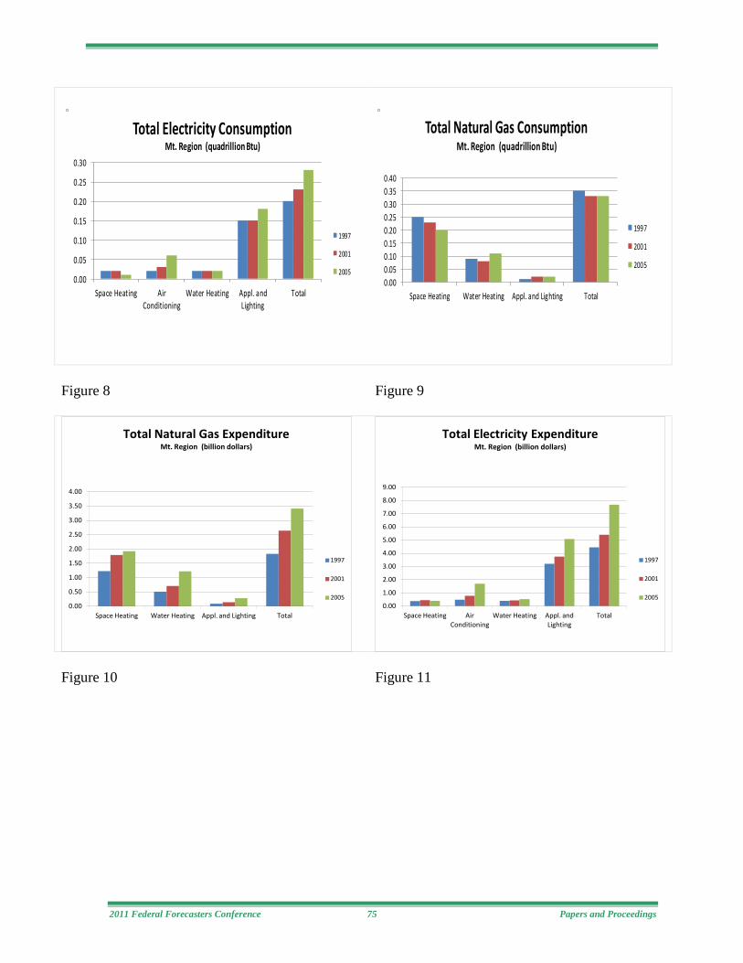
2011 Federal Forecasters Conference 75 Papers and Proceedings
Figure 8
Figure 9
Figure 10
Figure 11
0.00
0.05
0.10
0.15
0.20
0.25
0.30
Space Heating AirConditioning
Water Heating Appl. andLighting
Total
Total Electricity ConsumptionMt. Region (quadrillion Btu)
1997
2001
2005
0.00
0.50
1.00
1.50
2.00
2.50
3.00
3.50
4.00
Space Heating Water Heating Appl. and Lighting Total
Total Natural Gas Expenditure Mt. Region (billion dollars)
1997
2001
2005 0.00
1.00
2.00
3.00
4.00
5.00
6.00
7.00
8.00
9.00
Space Heating Air Conditioning
Water Heating Appl. and Lighting
Total
Total Electricity Expenditure Mt. Region (billion dollars)
1997
2001
2005
0.000.050.100.150.200.250.300.350.40
Space Heating Water Heating Appl. and Lighting Total
Total Natural Gas ConsumptionMt. Region (quadrillion Btu)
1997
2001
2005

2011 Federal Forecasters Conference 76 Papers and Proceedings
Intentionally blank

2011 Federal Forecasters Conference 77 Papers and Proceedings
Direct Marketing Strategies and Internet Connectivity Timothy Park and Shawn Wozniak
USDA, Economic Research Service, Farm and Rural Business Branch Paper prepared for presentation at the 18th Federal Forecasters Conference, Washington, D.C. April 2011
Abstract:
Initiatives to create an economically and environmentally sustainable food supply chain are an important driving force in the growth of direct marketing strategies (DMS), or local food sales, by farm operators, yet there is very little analysis that has examined motivation for producer participation. The U.S. Department of Agriculture (USDA) is also behind an initiative to increase the presence of broadband in rural areas of the United States. Those participating in direct marketing strategies are often reported on by journalists as young, new to farming, and internet-savvy. This study uses data from the 2008 Agricultural Resource Management Survey (ARMS) on direct marketing strategies used by farmers. Findings from this study suggest that obtaining an Internet connection and accessing the Internet for farm commerce is positively related to the likelihood of using intermediated marketing outlets. Using the Internet for farm commerce and operating diversified farms (more enterprises) is associated with increases in the likelihood that the farmer relies on direct to consumer marketing outlets.
1. Introduction
The community-based reorganization of the globalizing agro-food system into more localized food systems has been discussed and implemented over the last few decades as a means toward environmental and economic sustainability for consumers and producers, as well as a means toward greater food security and safety (Delind and Ferguson, 1999; La Trobe and Acott 2000; Norberg-Hodge 2002). Direct marketing strategies (DMS) have emerged and grown through outlets such as community supported agriculture farms (CSA) and buying clubs, farmers markets, on-farm and roadside stands, you-pick operations, consumer cooperatives, locally branded commodities as well as direct marketing to grocers and retailers (Kohls and Uhl, 1998; Buhr, 2004).
USDA’s “Know Your Farmer, Know Your Food” (KNF2) initiative builds on the 2008 Farm Act to strengthen Federal programs promoting local foods and includes plans to enhance direct marketing and farmers' promotion programs, to support local farmers and community food groups, to strengthen rural communities and to promote local eating. The KNF2
website (http://www.usda.gov/knowyourfarmer) lists opportunities for farm loan programs such as direct and guaranteed ownership loans for beginning farmers and socially disadvantaged groups, farm storage facility loans, value-added producer grants, beginning farmer and rancher development programs, and technical assistance and marketing services for farmers engaged in local selling.
Whole Foods, the world=s largest natural foods retailer, features its Locally Grown promise with a commitment to buying from local producers, particularly those who farm organically and are dedicated to environmentally sustainable agriculture. Produce that has traveled 7 or fewer hours by car or truck from the farm to the retail outlet can be labeled "locally grown." Wal-Mart offers local food vendors marketing assistance to supply its flagship stores and Sam's Clubs and presents training sessions to teach prospective suppliers how to win favor with Wal-Mart purchasers.
According to the 2007 Census of Agriculture, 136,817 farms implemented a form of a DMS an increase of 17 percent from 2002 (Detre, et al. 2010). Over the same period, farmers saw the value of direct marketing sales increase by 49 percent.
DMS allow producers to receive a better price by directly selling their products to consumers who have increasing demand for fresh and “local” food due to the growing concern for a healthier diet (Govindasamy et al. 1999, Morgan and Alipoe 2001, Uva 2002). Even lacking a clear definition of “local food” (Hand and Martinez, 2010; Martinez et al. 2010), some consumers are willing to pay more for locally grown products even after controlling for freshness (Darby et al. 2008). The initiative to create a sustainable food supply chain is another important driving force in the implementation of a DMS by farm operators (Ilbery and Maye 2005). Finally, since the majority of the food products sold through direct marketing channels is typically sourced locally instead of transported from national or international sources, direct marketing potentially mitigates the impact on the environment by reducing the carbon footprint in the food supply chain.
There is a plethora of literature on direct marketing strategies examining characteristics of consumers who buy directly from producers (Eastwood et al. 1987,

2011 Federal Forecasters Conference 78 Papers and Proceedings
Gallons et al. 1997, Govindasamy and Nayga 1997, Kezis et al. 1998, Kuches et al. 1999, Ladzinski and Toensmeyer 1983, Lehman et al. 1998, Schatzer et al. 1989, Thilmany and Watson 2004, Wolf 1997). Fewer studies exist that are focused on the production side (Brown et al. 2006, Detre et al. 2010, Govindasamy et al. 1999, Monson et al. 2008), examining producer behavior regarding DMS and how participation in DMS affects farm business income.
A review of literature reveals two overlooked aspects in the current literature on DMS. First, most studies are limited to a regional or state-level analysis. A broad motivation of this study is, therefore, to provide a comprehensive picture of DMS used in U.S. farming. In particular, we investigate the factors affecting choices of direct sales by farmers in (1)direct to consumer outlets (DTC), (2) intermediated outlets (IMO), and (3) both DTC and IMO outlets.
A secondary objective of this study is to assess the impact of choice of direct sales on the earnings intensity of the business. By examining the influence of choice of direct sales on earnings, the study can provide significant information to U.S. policy makers on factors influencing participation in local sales, especially whether the composition and use of the Internet influences farmer participation in direct sales. The analysis is conducted on a national farm-level basis with the unique feature of a large sample, comprising farms of different economic sizes, and in different regions of the United States.
The empirical approach is based on a discrete choice model where producers select a set of marketing channels to agricultural output. McFadden (1986) developed the economic choice theory underlying the multinomial logit model and highlighted its value in linking discrete choice behavior (choice of market outlet) with continuous decisions (sales revenue in each outlet). Ofek and Srinivasan (2002) demonstrated how market valuation of improved product attributes that account for competition from other brands, potential market expansion, and heterogeneous consumer preferences can be derived from the multinomial logit framework. We account for selectivity bias in the observed earnings from a marketing outlet, recognizing that producers choose from a set of marketing options to obtain the highest returns.
2. Econometric Model of Choice of Sales Outlets and Earnings in Chosen Outlet
Producers choose their marketing plans and assess outside options that are available before participating in any marketing channel.
The 2008 ARMS surveys queried farm operators on choices of sales (marketing) outlets and income earned when producers choose different market outlets to sell commodities. Based on this information, a set of three marketing outlets was identified. The marketing outlets included (1) DTC outlets only, (2) IMO only, and (3) both DTC and IMO outlets.
The producer’s choice of a marketing strategy is based on utility maximization among M alternatives, where utility depends on features of the outlets and the producer’s marketing expertise. The marketing strategies include the choice to market through any one outlet, any two outlets, all the outlets, or none of the outlets (no direct sales).
For producer i and marketing strategy j, the observed utility Uij in the additive random utility model is composed of a deterministic component, Vij and an unobserved random component eij:
ijijij VU ε+=
where Vij will depend on a set of explanatory variables Z and estimated parameters g.
Marketing strategy m is observed if alternative m has the highest utility across all the alternative strategies:
kVVkUU
kUUjy
ikijijim
ijim
ikiji
∀−≤−=
∀≤−=
∀≥==
)(Pr
),0(Pr
),(Pr)(Pr
εεwhere the Pr( yi = m) represents the probability of the event. The deterministic component is specified as
ijjiij ZV εγ +=
where the zi are case-specific regressors. If the unobserved random components are assumed to be identically and independently distributed with an identical extreme value distribution, the choice probabilities are
.,,1,)(exp
)(exp
),(Pr)(Pr
mjZ
ZkUUjy
lll
jj
ikiji
==
∀≥==
∑ γγ
As Cameron and Trivedi (2009) noted, gj is set to zero for one of the categories and coefficients are interpreted with respect to the omitted or base category.

2011 Federal Forecasters Conference 79 Papers and Proceedings
The MNL model offers a framework for dealing with selectivity effects in discrete choice models and has distinct theoretical and empirical advantages. Basuroy and Nguyen (1998) show that the MNL framework is appropriate for establishing equilibrium in market shares and assessing the impact of optimal firm responses to entry and potential market expansion. Choice models based on the MNL formulation are commonly used in marketing science applications and yield optimal pricing policies, which align with observed sales and pricing strategies of firms (Cattani, Dahan, and Schmidt, 2010). The parameters of the MNL model can be estimated by maximum likelihood techniques.
3. Data
The study employs data obtained from the nationwide 2008 Agricultural Resource Management Survey (ARMS) collected by the Economic Research Service (ERS) and the National Agricultural Statistics Service (NASS). The ARMS provides information about the relationships between agricultural production, resources, and the environment as well as about the characteristics and financial conditions of farm households, management strategies, and off-farm income. Data are collected from the senior farm operator per farm, who makes most of the day-to-day management decisions. For the purpose of this study, we excluded operator households organized as nonfamily corporations or cooperatives and farms run by hired managers.
Operators associated with farm businesses representing agricultural production in the 48 contiguous states make up the target population of the survey. USDA defines a farm as an establishment that sold or normally would have sold at least $1,000 of agricultural products during the year. Farms may be organized as sole proprietorships, partnerships, or family corporations. In addition to farm economic data, the 2008 ARMS also collected information on farm households. It contains detailed information on off-farm hours worked by spouses and farm operators, the amount of income received from off-farm work, net cash income from operating another farm/ranch, net cash income from operating another business, and net income from share renting.
The 2008 ARMS queried farm operators on choices of sales (marketing) outlets and income earned when producers choose different market outlets to sell commodities. The survey instrument contains specific questions pertaining to the use of direct marketing
strategy by farmers. Specifically, the survey queried farmers whether they have used the following direct marketing outlets: (1) roadside stand or on-farm facility, (2) on-farm stores, (3) farmers’ markets, (4) community supported agriculture (CSA), (5) regional distributors, (6) state branding programs, and (7) direct sales to local grocery stores, restaurants and other retailers. Based on this information, a set of three marketing outlets was identified.
Choices 1 through 4 were grouped into DTC and include ten percent of producers. Choices 5 through 7 were grouped into IMO and account for seven percent of producers. The third group includes farmer who used both DTC and IMO outlets, and includes four percent of the producers. Farms with no direct sales outlets were used as the base group and comprise 79 percent of the farms in the 2008 ARMS dataset.
Figures 1 and 2 show violin plots of total value of farm sales by participation in direct marketing and by DMS choice. Violin plots combine box plots and density traces in one diagram. The box plots display the center, the spread, asymmetry and outliers in data while the density traces reveal the distribution of the data, with its valleys, peaks and bumps. The mean for farmers participating in any form of direct sales is just under $500,000 for net value of farm sales, while the mean for those not participating is somewhat higher.
The plot demonstrates that there are a larger number of small farms participating compared to large farms, but large farms participating show higher net value sales overall. There is a large standard deviation for participants and non-participants, suggesting some volatility in participation. Farmers participating in DTC are skewed in the plot mostly toward the left, with the median being under $100,000 for net farm sales. There are three nodes, heavy in the lower group, and slight for farms in the middle and higher net value of sales areas. For IMO only, there are two almost symmetrical nodes, showing almost equal participation by small and large farmers, while those having mixed strategies mostly skew toward farmers with lower net value of farm sales.
4. Results and Discussion
Table 1 reports descriptive statistics of the independent variables. Table 2 reports parameter estimates of the choice of direct marketing model used by farmers in the US. Note that the base group for comparison is farmers with no direct marketing sales. We focus our discussion on a few key explanatory variables.
The ARMS provides information about the locations used by farmers to connect to the Internet including
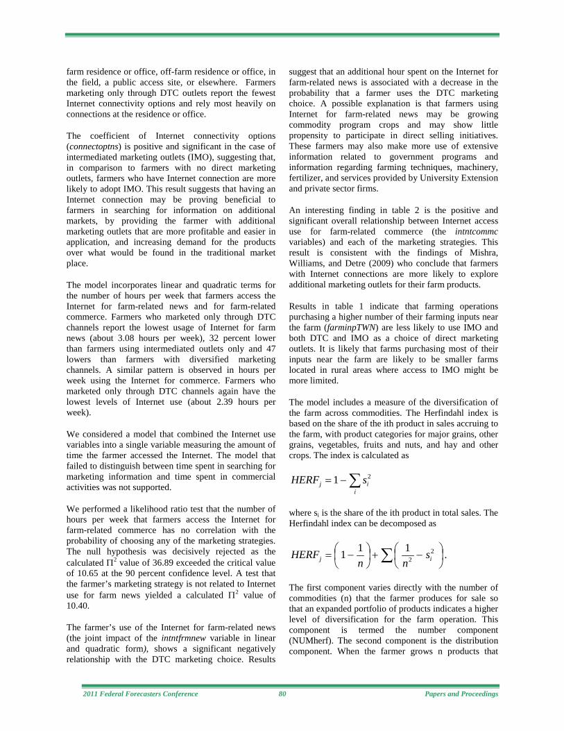
2011 Federal Forecasters Conference 80 Papers and Proceedings
farm residence or office, off-farm residence or office, in the field, a public access site, or elsewhere. Farmers marketing only through DTC outlets report the fewest Internet connectivity options and rely most heavily on connections at the residence or office.
The coefficient of Internet connectivity options (connectoptns) is positive and significant in the case of intermediated marketing outlets (IMO), suggesting that, in comparison to farmers with no direct marketing outlets, farmers who have Internet connection are more likely to adopt IMO. This result suggests that having an Internet connection may be proving beneficial to farmers in searching for information on additional markets, by providing the farmer with additional marketing outlets that are more profitable and easier in application, and increasing demand for the products over what would be found in the traditional market place.
The model incorporates linear and quadratic terms for the number of hours per week that farmers access the Internet for farm-related news and for farm-related commerce. Farmers who marketed only through DTC channels report the lowest usage of Internet for farm news (about 3.08 hours per week), 32 percent lower than farmers using intermediated outlets only and 47 lowers than farmers with diversified marketing channels. A similar pattern is observed in hours per week using the Internet for commerce. Farmers who marketed only through DTC channels again have the lowest levels of Internet use (about 2.39 hours per week).
We considered a model that combined the Internet use variables into a single variable measuring the amount of time the farmer accessed the Internet. The model that failed to distinguish between time spent in searching for marketing information and time spent in commercial activities was not supported.
We performed a likelihood ratio test that the number of hours per week that farmers access the Internet for farm-related commerce has no correlation with the probability of choosing any of the marketing strategies. The null hypothesis was decisively rejected as the calculated Π2 value of 36.89 exceeded the critical value of 10.65 at the 90 percent confidence level. A test that the farmer’s marketing strategy is not related to Internet use for farm news yielded a calculated Π2 value of 10.40.
The farmer’s use of the Internet for farm-related news (the joint impact of the intntfrmnew variable in linear and quadratic form), shows a significant negatively relationship with the DTC marketing choice. Results
suggest that an additional hour spent on the Internet for farm-related news is associated with a decrease in the probability that a farmer uses the DTC marketing choice. A possible explanation is that farmers using Internet for farm-related news may be growing commodity program crops and may show little propensity to participate in direct selling initiatives. These farmers may also make more use of extensive information related to government programs and information regarding farming techniques, machinery, fertilizer, and services provided by University Extension and private sector firms.
An interesting finding in table 2 is the positive and significant overall relationship between Internet access use for farm-related commerce (the intntcommc variables) and each of the marketing strategies. This result is consistent with the findings of Mishra, Williams, and Detre (2009) who conclude that farmers with Internet connections are more likely to explore additional marketing outlets for their farm products.
Results in table 1 indicate that farming operations purchasing a higher number of their farming inputs near the farm (farminpTWN) are less likely to use IMO and both DTC and IMO as a choice of direct marketing outlets. It is likely that farms purchasing most of their inputs near the farm are likely to be smaller farms located in rural areas where access to IMO might be more limited.
The model includes a measure of the diversification of the farm across commodities. The Herfindahl index is based on the share of the ith product in sales accruing to the farm, with product categories for major grains, other grains, vegetables, fruits and nuts, and hay and other crops. The index is calculated as
∑−=i
ij sHERF 21
where si is the share of the ith product in total sales. The Herfindahl index can be decomposed as
.111 22∑
−+
−= ij s
nnHERF
The first component varies directly with the number of commodities (n) that the farmer produces for sale so that an expanded portfolio of products indicates a higher level of diversification for the farm operation. This component is termed the number component (NUMherf). The second component is the distribution component. When the farmer grows n products that

2011 Federal Forecasters Conference 81 Papers and Proceedings
comprise equal shares of total sales, then the distribution component is zero indicating an equal distribution across the products. Higher negative values reveal that the distribution of sales shares across products is increasingly unequal and the farm operation is less diversified. The distribution component is identified as DISTherf.
Results in table 2 indicate a positive and significant association between the number of crops grown by the farm and choice of direct marketing outlets. In particular, the coefficient of NUMherf is positive and significant for DTC and both DTC and IMO marketing outlets, when compared to the base group (no direct marketing sales). A higher Herfindahl index indicates a diversified farm and it can be argued that diversified farms are seeking several marketing outlets, including direct sales (DTC) and intermediated outlets (IMO).
The Herfindahl index results when the number component and the distribution component are combined. The decomposition that is used in the multinomial logit model provides more information to assess how diversification across agricultural products is related to choice of marketing strategy. The marketing strategy choice is more closely related to the producer’s decision on the portfolio of crops to grow and market rather than the magnitude of the sales shares that are claimed by each crop. A model that combines the number and distribution components of the Herfindahl index into a single variable is rejected as the calculated Π2 value of 26.96 exceeds the critical value of 4.60 at the 90 percent confidence level.
Beginning farmers (begfarmer), those who began farming after 1997, are more likely to choose DTC as their choice of direct marketing strategy. The finding here suggests that entrants in farming may be more educated and are likely to engage in off-farm work (Mishra et al. 2002). The new entrants are more likely to operate small and diversified farms, located near metro-areas, where the demand for local food items and fresh produce is greater than for farms located in more sparely populated areas.
5. Conclusions
In the era of a global economy, farmers face increasing pressure in developing a portfolio of various marketing channels and in bargaining competitively with increasingly sophisticated marketing participants in the supply chain of agricultural products in local and regional markets. Many farmers begin selling directly through farmers’ markets, roadside stands, community supported agriculture. Regional distributors, state branding programs, direct sales to grocery stores, local
restaurants, and other retailers represent another set of available outlets. This research assists producers by examining direct marketing strategies and identifies specific farm and demographic factors that are associated with the choice of direct marketing outlets.
Results from the discrete model (multinomial logit model) highlight variables that may influence the choice of direct marketing outlets by farmers in the U.S. Extension agents, crop consultants, and marketing analysts can adapt this information to predict the type of marketing outlet that a given farmer might use and provide better information for farmers. Getting an Internet connection and using the Internet for farm commerce, increases the likelihood that a farmer uses intermediated marketing outlets (IMO).
On the other hand, using the Internet for farm commerce and growing a diversified selection of products (more enterprises) increases the likelihood that a farmer uses direct to consumer marketing outlets (DTC). Using the Internet for farm related news decreases the likelihood of participation in direct to consumer marketing outlets (DTC). Finally, farming operations purchasing a higher number of their farming inputs near the farm are less likely to use IMO and both DTC and IMO as a choice of direct marketing outlets.
References
Cattani, K.D., Dahan, E., Schmidt, G. Spackling: “Lowest Cost May Not Lower Total Cost: Using ‘Spackling to Smooth Mass-Customized Production.” Production & Operations Management 19, 5: 531-545, 2010.
Brown, C., J. E. Gandee, and G. D'Souza. “West Virginia Farm Direct Marketing: A County Level Analysis.” Journal of Agricultural and Applied Economics 38, 3 (2006).
Brown, C., and S. Miller. “The Impacts of Local Markets: A Review of Research on Farmers Markets and Community Supported Agriculture (CSA).” American Journal of Agricultural Economics 90, 5: 1296-302 (2008).
Buhr, B. L. “Case Studies of Direct Marketing Value-Added Pork Products in a Commodity Market.” Review of Agricultural Economics 26, 2, 266-79 (2004).
Cameron, A.C. and P.K. Trivedi.. “Microeconometrics Using Stata..” College Station, TX: Stata Press, 2009.

2011 Federal Forecasters Conference 82 Papers and Proceedings
Darby, K., M. T. Batte, S. Ernst, and B. Roe. “Decomposing Local: A Conjoint Analysis of Locally Produced Foods.” American Journal of Agricultural Economics, 90, 476-86 (2008).
Delind, L. B., and A. Ferguson. “Is This a Women’s Movement? The Relationship of Gender to Community-Supported Agriculture in Michigan,” Human Organization, 58, 2, 190-200 (1999)
Detre, J., T. Mark., A. Mishra, and A. Adhikari. “Linkage between Direct Marketing and Farm Income: Double Hurdle Approach.” Agribusiness: an International Journal, 27, 1, 19-33 (2011).
Eastwood, D. B., J. R. Brooker, and R. H. Orr. “Consumer Preferences for Local Versus out-of-State Grown Selected Fresh Produce: The Case of Knoxville, Tennessee.” Southern Journal of Agricultural Economics 19, 2 (1987).
Gallons, J., U. C. Toensmeyer, J. R. Bacon, and C. L. German. “An Analysis of Consumer Characteristics Concerning Direct Marketing of Fresh Produce in Delaware: A Case Study." Journal of Food Distribution Research 28, 1 (1997).
Govindasamy, R., F. Hossain, and A. Adelaja. “Income of Farmers Who Use Direct Marketing.” Agricultural and Resource Economics Review 28, 1 76-83 (1999).
Govindasamy, R. and R. M. Nayga, Jr. “Determinants of Farmer-to-Consumer Direct Market Visits by Type of Facility: A Logit Analysis.” Agricultural and Resource Economics Review 26, 1 (1997).
Hand, M. S., and S. Martinez. “Just What Does Local Mean?” Choices 25, 1 (2010).
Ilbery, B., and D. Maye. “Food Supply Chains and Sustainability: Evidence from Specialist Food Producers in the Scottish/English Borders.” Land Use Policy 22, 4, 331-44 (2005).
Kezis, A., T. Gwebu, S. Peavey, and H-Tai Cheng. “A Study of Consumers at a Small Farmers' Market in Maine: Results from a 1995 Survey.” Journal of Food
Distribution Research 29, 1 (1998).
Kohls, R. L. and J.N. Uhl. “Marketing of Agricultural Products.” 8 ed. Englewood Cliffs, NJ: Prentice Hall, 1998.
Kuches, K., U. C. Toensmeyer, C. L. German, and J. R. Bacon. “An Analysis of Consumers' Views and Preferences Regarding Farmer to Consumer Direct Markets in Delaware.” Journal of Food Distribution Research 30, 1 (1999).
Ladzinski, K., and U. C. Toensmeyer. “Importance of Direct Markets for Consumers in Their Fresh Vegetable and Fruit Purchases.” Journal of Food Distribution Research 14, 3 (1983).
La Trobe, H.L., and T.G. Acott. “Localising the Global Food System,” International Journal of Sustainable Development and World Ecology, 7, 309-320 (2000).
Lehman, J., J. R. Bacon, U. Toensmeyer, J. Pesek, and C. German. “An Analysis of Consumer Preferences for Delaware Farmer Direct Markets.” Journal of Food Distribution Research 29, 1 (1998).
Martinez, S., M. Hand, M. Da Pra, S. Pollack, K. Ralston, T. Smith, S. Vogel, S. Clark, L. Lohr, S. Low, and C. Newman. “Local Food Systems. Concepts,
Impacts and Issues.” Economic Research Report 97 (2010).
McFadden, D. “The Choice Theory Approach to Market Research.” Marketing Science 5, 275-297 (1986).
Monson, J., D. Mainville, and N. Kuminoff. “The Decision to Direct Market: An Analysis of Small Fruit and Specialty-Product Markets in Virginia.” Journal of Food Distribution Research 39, 2, 1-11 (2008).
Morgan, T. K., and D. Alipoe. “Factors Affecting the Number and Type of Small-Farm Direct Marketing Outlets in Mississippi.” Journal of Food Distribution Research 32, 1 (2001).
Norberg-Hodge, H. “Think Global...Eat Local.” Ecologist, 32, 7, 28-31 (2002).
Ofek, E. and V. Srinivasan. “How Much Does the Market Value an Improvement in a Product Attribute?” Marketing Science 21, 398-411 (2002).
Payne, Tim. “U.S. Farmers' Markets 2000: A Study of Emerging Trends.” Journal of Food Distribution Research 33, 1 (2002).
Schatzer, R., D. S. Tilley, and D. Moesel. “Consumer Expenditures at Direct Produce Markets.” Southern Journal of Agricultural Economics 21, 1 (1989).

2011 Federal Forecasters Conference 83 Papers and Proceedings
Thilmany, D., and P. Watson. “The Increasing Role of Direct Marketing and Farmers Markets for Western US Producers.” Western Economics Forum 3, 2 (2004).
Uva, Wen-Fei L. "An Analysis of Vegetable Farms' Direct Marketing Activities in New York State." Journal of Food Distribution Research 33, 1 (2002).
Varner, T., and D. Otto. “Factors Affecting Sales at Farmers' Markets: An Iowa Study.” Review of Agricultural Economics 30, 1, 176-189 (2008).
Wolf, M. “A Target Consumer Profile and Positioning for Promotion of the Direct Marketing of Fresh Produce: A Case Study.” Journal of Food Distribution Research 28, 3 (1997).

2011 Federal Forecasters Conference 84 Papers and Proceedings
Table 1: Variable Definition and Summary Statistics Variable Description Direct-to-Consumers
(DTC) outlets1 Intermediated (IMO) outlets2
DTC & IMO3
Mean (Std. Dev)
Mean (Std. Dev)
Mean (Std. Dev)
connectoptns Internet connectivity options 1.0536
(0.8020) 1.2262
(0.9521) 1.2021
(0.9225) intntfrmnews Internet used for farm-related news (hours/week) 3.9157
(6.4432) 5.1429
(7.7012) 5.7447
(8.3123) intntcommc Internet used for farm-related commerce (hours/week) 3.5785
(8.0845) 5.2560
(9.9880) 6.0319
(10.8086) farminpTWN Inputs available near farm (count of five inputs)1 2.2375
(1.7773) 2.0774
(1.6953) 2.0426
(1.6779) hldcongdTWN Household consumer good available for purchase near farms (=1 if
good available, otherwise)2 0.3372
(0.4736) 0.3512
(0.4787) 0.3298
(0.4726) hlddurgdTWN Household durable good available for purchase near farms (=1 if
goods available, otherwise)3 0.2414
(0.4287) 0.2321
(0.4236) 0.2234
(0.4188) DISTherf Distribution component of Herfindahl index for crops sold by the
producer 0.1009
(0.1913) 0.0981
(0.2039) 0.1444
(0.2293) NUMherf Number component of Herfindahl index for crops sold by the
producer 0.1762
(0.2629) 0.1592
(0.2488) 0.2367
(0.2760) begfarmer Operator began operating this farm after 1997 0.1686
(0.3751) 0.1369
(0.3447) 0.1277
(0.3355) tvalfrmsal Total value of farm sales in 2008 395,112
(540,689) 636,448
(606,732) 539,853
(561,576) Sample size
261 168 94
1 Includes fuel, fertilizer and chemicals, feed and seed, machinery and implements, farm credit. 2 Includes groceries, clothing, household supplies, etc. 3 Includes cars, trucks, appliances, furniture, etc. Source: Agricultural and Resource Management Survey, USDA Economic Research Service and NASS, 2008.

2011 Federal Forecasters Conference 85 Papers and Proceedings
Table 2: Parameter estimates for multinomial logit model of direct marketing strategy Variable DTC Only t-value IMO Only t-value
Both DTC and IMO t-value
Constant -2.468* 13.413 -3.367* 13.153 -3.525* 14.159
(0.184)
(0.256)
(0.249)
connectoptns 0.073 -0.602 0.349* -2.494 0.108 -0.768
(0.122)
(0.140)
(0.140)
Frmnews -0.109* 2.869 -0.070 1.451 -0.037 0.897
(0.038)
(0.048)
(0.041)
commc 0.068* -1.800 0.088* -2.004 0.118* -3.193
(0.038)
(0.044)
(0.037)
farminpTWN -0.040 0.737 -0.172* 2.096 -0.126* 1.725
(0.054)
(0.082)
(0.073)
hldconsgdTWN -0.258 1.061 0.356 -1.018 -0.148 0.449
(0.243)
(0.350)
(0.330)
hlddurgdTWN 0.009 -0.036 -0.215 0.593 0.064 -0.190
(0.248)
(0.363)
(0.339)
DISTherf -1.064 1.41 0.514 0.43 0.433 0.56
(0.754)
(1.207)
(0.775)
NUMherf 0.854* 1.74 -1.009 -1.09 2.736* 5.29
(0.489)
(0.973)
(0.518)
begfarmer 0.745* -3.515 0.406 -1.199 0.380 -1.160
(0.212)
(0.339)
(0.328)
frmnews2 0.002* -2.431 0.002* -1.776 0.001 -1.196
(0.001)
(0.001)
(0.001)
commc2 -0.001 0.879 -0.001 0.994 -0.001 1.105
(0.001)
(0.001)
(0.001)
a Standard error of explanatory variables in parentheses. b Asterisk indicates asymptotic t-values with significance at α = 0.10 or higher level.

2011 Federal Forecasters Conference 86 Papers and Proceedings
Figure 1: Violin Plot of Farm Sales by DMS Participation
Source: Agricultural and Resource Management Survey, USDA Economic Research Service and NASS, 2008 Figure 2: Violin Plot of Farm Sales by DMS
Source: Agricultural and Resource Management Survey, USDA Economic Research Service and NASS, 2008

2011 Federal Forecasters Conference 87 Papers and Proceedings
Figure 3: Internet Use by Direct Marketing Choice
Source: Agricultural and Resource Management Survey, USDA Economic Research Service and NASS, 2008

2011 Federal Forecasters Conference 88 Papers and Proceedings
Intentionally blank

2011 Federal Forecasters Conference 89 Papers and Proceedings
Forecasting Dynamics of the Economy
Session Chair: Kathryn Byun, Bureau of Labor Statistics, U.S. Department of Labor
Compositional Differences in Gross Domestic Product (GDP) Estimates Between Recession and Expansions Tara M. Sinclair and H.O. Stekler, The George Washington University
The main topic of this paper is to determine whether data revisions could influence forecasting because the composition of GDP varies substantially from one vintage of data to another. We introduce a number of new statistics for measuring the magnitude of these compositional changes. We further specifically investigate the potential role of changes in the state of the economy for these compositional changes. Our analysis shows that the early data generally reflected the composition of the changes in GDP that was observed in the later data. Thus, under most circumstances, an analyst could use the early data to obtain a realistic picture of what had happened in the economy in the previous quarter. However, the differences in the composition of the vectors of the two vintages were larger during recessions than in expansions. Unfortunately, it is in those periods when accurate information is most vital for forecasting.
Assessing Global Vector Auto-Regressions for Forecasting Neil R. Ericsson and Erica L. Reisman; Federal Reserve Board (Paper following)
Global vector auto-regressions (GVARs) have several attractive features: a standardized economically appealing choice of variables for each country or region examined a systematic treatment of long-run properties, and flexible dynamic specification. Pesaran, Schuermann, and Smith (2009) generate and evaluate forecasts from a paradigm GVAR with 26 countries. The current paper empirically assesses that GVAR with impulse indicator saturation, a new generic procedure for evaluating parameter constancy---a central element in model-based forecasting. The results indicate substantial room for an improved, more robust specification of that GVAR, with some tests suggestive of how to achieve such improvements.

2011 Federal Forecasters Conference 90 Papers and Proceedings
Intentionally blank

2011 Federal Forecasters Conference 91 Papers and Proceedings
Assessing Global Vector Auto-Regressions for Forecasting Neil R. Ericsson
Division of International Finance, Federal Reserve Board, Washington, DC 20551 Research Program on Forecasting, Department of Economics, The George Washington University
and
Erica L. Reisman Division of International Finance, Federal Reserve Board
ABSTRACT Global vector autoregressions (GVARs) have several attractive features: multiple potential channels for the international transmission of macroeconomic and financial shocks, a standardized economically appealing choice of variables for each country or region examined, systematic treatment of long-run properties through cointegration analysis, and flexible dynamic specification through vector error correction modeling. Pesaran, Schuermann, and Smith (2009) generate and evaluate forecasts from a paradigm GVAR with 26 countries, based on Dées, di Mauro, Pesaran, and Smith (2007). The current paper empirically assesses the GVAR in Dées, di Mauro, Pesaran, and Smith (2007) with impulse indicator saturation (IIS)—a new generic procedure for evaluating parameter constancy, which is a central element in model-based forecasting. The empirical results indicate substantial room for an improved, more robust specification of that GVAR. Some tests are suggestive of how to achieve such improvements. Keywords: cointegration, error correction, forecasting, GVAR, impulse indicator saturation, model design, model evaluation, model selection, parameter constancy, VAR. JEL codes: C32, F41. Acknowledgements: The authors are a staff economist and a research assistant in the Division of International Finance, Board of Governors of the Federal Reserve System, Washington, DC 20551 USA; and they may be reached on the Internet at [email protected] and [email protected] respectively. The views in this paper are solely the responsibility of the authors and should not be interpreted as reflecting the views of the Board of Governors of the Federal Reserve System or of any other person associated with the Federal Reserve System. The authors are grateful to David Hendry, Jesper Lindé, Filippo di Mauro, Hashem Pesaran, Tara Rice, and Vanessa Smith for helpful discussions and comments; and additionally to Vanessa Smith for invaluable guidance in replicating estimation results from Dées, di Mauro, Pesaran, and Smith (2007). All numerical results were obtained using PcGive Version 13.10 and Autometrics Version 1.5e in OxMetrics 6.10:
see Doornik and Hendry (2009) and Doornik (2009). 1. INTRODUCTION The recent financial crisis and ensuing Great Recession have highlighted the importance and pervasiveness of international linkages in the world economy—and the importance of capturing those linkages in empirical macroeconomic models that are used for economic analysis, forecasting, and policy analysis. Pesaran, Schuermann, and Weiner (2004) propose and implement global vector autoregressions (or GVARs) as an ingenious approach for capturing international linkages between country- or region-specific error correction models. Dées, di Mauro, Pesaran, and Smith (2007) (hereafter DdPS) extend that work to a larger number of countries and regions; and Pesaran, Schuermann, and Smith (2009) assess the forecasting properties of the GVAR implemented in DdPS. The GVAR methodology has several attractive features:
a versatile structure for characterizing inter-national macroeconomic and financial linkages though multiple channels,
a standardized economically appealing choice of variables (both domestic and foreign) for each country or region,
a systematic treatment of long-run properties through cointegration analysis, and
flexible dynamic specification through vector error correction modeling.
These features are very appealing, and they balance naturally the roles of data and economic theory in empirical modeling. The GVAR explicitly aims to capture international economic linkages, especially linkages between the macroeconomic and financial sides of economies. Weak exogeneity plays an important role through allowing conditional subsystem analysis on a country-by-country basis. Data aggregation—empirically implemented but based on economic theory—achieves a high degree of parsimony in the estimated models. The current paper re-examines some of the empirical underpinnings for global vector autoregressions, focusing on parameter constancy because of the intimate
2011 Federal Forecasters Conference 92 Papers and Proceedings
connections between it and forecast performance. To test parameter constancy, this paper uses impulse indicator saturation, which is a recent generic approach to evaluating constancy. The empirical results indicate substantial room for an improved, more robust specification of DdPS’s GVAR; and some tests are suggestive of how to achieve such improvements. See Clements and Hendry (1998, 1999, 2002) and Hendry (2006) for discussions on the relationships between parameter constancy, forecast performance, and forecast failure. In related work, Ericsson (2011) discusses the theory of reduction and exogeneity in the context of GVARs, thereby providing the background for tests of parameter constancy, data aggregation, and weak exogeneity in GVARs. Using those tests, Ericsson (2011) then evaluates the equations for the United States, the euro area, the United Kingdom, and China in DdPS’s GVAR. Ericsson and Reisman (2011) provide parallel results for equations for all 26 countries in DdPS’s GVAR. This paper is organized as follows. Section 2 describes a prototypical GVAR and, in the context of that prototypical GVAR, summarizes the current approach taken to modeling GVARs, as developed in Pesaran, Schuermann, and Weiner (2004) and DdPS inter alia. Section 3 reviews the procedure for testing parameter constancy called impulse indicator saturation, which utilizes the computer-automated model selection algorithm in Autometrics. Section 4 empirically evaluates DdPS’s GVAR for parameter constancy, using impulse indicator saturation. Section 5 concludes. 2. THE GVAR To motivate the use of GVARs in practice, this section describes a prototypical GVAR (Section 2.1) and relates it to the GVAR in DdPS (Section 2.2). The current approach to modeling GVARs has been developed in Pesaran, Schuermann, and Weiner (2004) and DdPS inter alia. For further research on GVARs, see Garratt, Lee, Pesaran, and Shin (2006); Pesaran and Smith (2006); Dées, Holly, Pesaran, and Smith (2007); Pesaran, Smith, and Smith (2007); Hieberta and Vansteenkiste (2009); Pesaran, Schuermann, and Smith (2009); Castrén, Dées, and Zaher (2010); Chudik and Pesaran (2011); and the comments and rejoinders to Pesaran, Schuermann, and Weiner (2004) and Pesaran, Schuermann, and Smith (2009). Juselius (1992) provides a conceptual precursor to GVARs in her sector-by-sector analysis of the Danish economy to obtain multiple long-run feedbacks entering an equation for domestic inflation. Smith and Galesi (2010) have designed and documented an easy-to-use Excel-based interface that accesses Matlab procedures to implement GVARs.
2.1. A Prototypical GVAR This subsection describes a prototypical GVAR that has three countries, with two variables per country and a single lag on each variable in the underlying vector autoregression (VAR). For ease of exposition, global variables (such as oil prices) and deterministic variables (such as an intercept and trend) are ignored. This prototypical GVAR highlights key features that are important to the remainder of this paper. In the exposition below, this prototypical GVAR is considered first in its generic form, then in its error correction representation, then on a country-by-country basis, and finally on a variable-by-variable basis for each country. While the prototypical GVAR may well be unreal-istically simple for empirical use, it conveys important aspects of the GVAR without undue algebraic com-plication, and it allows (in Section 2.2) a straightforward description of the GVAR in DdPS. Ericsson (2011) provides a more complete description of the structure of GVARs, the notation used, and the underlying assumptions. The underlying VAR for the prototypical GVAR is:
(1) ,
for 0,1,2, and 1,2, … , , where is the country index, is the time index, is the number of observations, is the vector of domestic variables for country at time , is the vector of corresponding foreign aggregates (i.e., foreign relative to country ) at time , is the matrix of coefficients on the lagged domestic variables, and are the matrices of coefficients on the contemporaneous and lagged foreign aggregates, and is the error term induced by having conditioned on those foreign variables. Empirically, one interesting triplet of countries is as follows: the United States ( 0), the euro area ( 1), and China ( 2). Each subsystem in (1) is also a VARX* model—that is, a VAR model that conditions on a set of (assumed) exogenous variables and their lags. In error correction representation, the prototypical GVAR in (1) is:
(2) Δ Γ Δ : ,
for 0,1,2, and 1,2, … , , where Δ is the difference operator, Γ is the matrix of coefficients on the change in contemporaneous foreign aggregates, and and are the matrices of adjustment coefficients and cointegrating vectors for country . The matrices Γ , , and in (2) are functions of the matrices , , and
in (1). The explicit country-by-country structure of the GVAR in equation (2) is as follows:

2011 Federal Forecasters Conference 93 Papers and Proceedings
(3) Δ Γ Δ :
Δ Γ Δ :
Δ Γ Δ : .
In equation (3), a country’s domestic variables respond to the foreign aggregates and to lagged disequilibria involving the domestic and foreign variables. Country 0’s foreign aggregate is a weighted sum of and , which are the foreign variables for country 0. Likewise, is a weighted sum of and , and is a weighted sum of and . The weights might be chosen to reflect the relative economic importance of the foreign countries to the domestic country. So, the weights for one country’s foreign aggregates need not (and generally would not) be the same as the weights for another country’s foreign aggregates. To further illuminate the structure of the GVAR, sup-pose that in equation (3) comprises two variables: (the log of country ’s real GDP), and Δ (country ’s CPI inflation). Because : Δ and
: Δ , equation (3) can thus be written explicitly in six equations.
(4) Δ Γ Δ Γ Δ
: Δ : : Δ
Δ Γ Δ Γ Δ
: Δ : : Δ
Δ Γ Δ Γ Δ
: Δ : : Δ
Δ Γ Δ Γ Δ
: Δ : : Δ
Δ Γ Δ Γ Δ
: Δ : : Δ
Δ Γ Δ Γ Δ
: Δ : : Δ
The subscripts and refer to the two variables and Δ . The GVAR itself is thus a vector error correction model in which the individual conditional error correction models for all of the countries are stacked, one on top of the other. Consider the interpretation of (4). In the first equation of (4), the growth of GDP in country 0 depends on the growth of GDP and inflation in countries 1 and 2 through Δ and Δ , and on lagged disequilibria involving both domestic and foreign variables through the cointegrating relationships : Δ : : Δ . In each remaining equation, the domestic variable likewise depends on the foreign variables through the
change in their contemporaneous aggregates and through the error correction term. Some potential cointegrating vectors include the following, where denotes a generic cointegrating vector and a diamond ♦ denotes a nonzero coefficient.
i. 1: 0: : 0 : domestic and foreign GDP are cointegrated.
ii. 1: : 0: 0 : domestic GDP is cointegrated with domestic inflation.
iii. 1: 0: 0: 0 : domestic GDP is stationary, or is trend-stationary if a trend is included in the cointegrating space.
iv. 0: 1: 0: : domestic and foreign inflation are cointegrated.
v. 0: 1: 0: 0 : domestic inflation is stationary.
Even in this simple two-variable example, many long-run relationships are possible. Yet more (and more complicated) long-run relationships may exist in multi-variate settings such as the GVAR in DdPS, described in Section 2.2. While the prototypical GVAR in (4) has a remarkable simplicity of structure, it still shows how domestic and foreign variables may influence each other through multiple channels, and in both the short run and the long run. As (4) illustrates, a GVAR provides a versatile structure for characterizing multiple international linkages for a standardized economically appealing choice of variables with a systematic and flexible treatment of long-run and short-run properties through cointegration analysis and vector error correction modeling. In practice, GVARs have many potential uses, such as private-firm policy regarding risk, banking supervision and regulation, central bank policy, and forecasting; cf. Pesaran, Schuermann, and Weiner (2004), Dées, di Mauro, Pesaran, and Smith (2007), and Pesaran, Schuermann, and Smith (2009). In some of these situations, strong exogeneity, super exogeneity, or both may be required for valid analysis; see Ericsson, Hendry, and Mizon (1998) and Ericsson (2011). 2.2. The GVAR in DdPS To provide a sense of the empirical aspects involved in modeling a global vector autoregression, consider the GVAR in DdPS. The set of domestic variables is as follows (with a few exceptions for specific countries, as noted in DdPS):
Real GDP ( ),
CPI inflation (Δ ),

2011 Federal Forecasters Conference 94 Papers and Proceedings
Real equity prices ( ),
Real exchange rate ( ),
Short-term interest rate ( ), and
Long-term interest rate ( ).
DdPS focus on 25 countries plus one region (the euro area); see Table 2 in Section 4.2 for a list of the countries. For convenience, both countries and regions are referred to as “countries” below. The country-specific aggregated foreign variables ( ) are constructed from the full set of domestic variables across all countries, using fixed trade weights. The VARX* for each country initially has two lags on domestic variables and on the foreign aggregates. In some instances, however, shorter lags are selected, based on standard information criteria. Also, the VARX* includes a global variable (oil prices) and deterministic variables (an intercept and trend). Cointegration in the VARX* is tested, following the procedure in Harbo, Johansen, Nielsen, and Rahbek (1998) and using critical values from MacKinnon, Haug, and Michelis (1999); see also Johansen (1992, 1995) and Juselius (2006). The number of cointegrating vectors may differ from country to country. In the conditional error correction model, the country’s cointegrating vectors are written in their reduced form, i.e., with beginning with an identity matrix. The data are quarterly, taken from the IMF’s International Financial Statistics (except for Sing-apore’s data, which are from Datastream). Estimation is typically over 1979Q4–2003Q4 ( 97). This GVAR from DdPS provides the empirical illustration examined in Section 4. 3. IMPULSE INDICATOR SATURATION This section describes the procedure called impulse indicator saturation, which Section 4 uses to test parameter constancy of the GVAR in DdPS. Impulse indicator saturation (IIS) uses zero-one impulse indicator dummies to analyze properties of a model. There are such dummies, one for each observation in the sample. While inclusion of all dummies in an estimated model is infeasible, blocks of dummies can be included; and that insight provides the basis for IIS. A simple example with two equal-sized blocks motivates the generic approach in IIS. See Hendry, Johansen, and Santos (2008), Johansen and Nielsen (2009), and Hendry and Santos (2010) for further discussion and recent developments. Imagine estimating a model specification such as the
GVAR in (4) in three steps. First, estimate that model, including impulse indicator dummies for the first half of the sample. That estimation is equivalent to estimating the model over the second half of the sample, ignoring the first half. Drop all statistically insignificant impulse indicator dummies and retain the statistically significant dummies. Second, repeat this process, but start by including impulse indicator dummies for the second half of the sample; and retain the statistically significant ones. Third, re-estimate the original model, including all dummies retained in the two block searches; and select the statistically significant dummies from that combined set. Hendry, Johansen, and Santos (2008) and Johansen and Nielsen (2009) have shown that, under the null hypothesis of correct specification, the fraction of impulse indicator dummies retained is roughly , where is the target size. For instance, if 100 and the target size is 1%, then (on average) only one impulse indicator dummy is retained when the model is correctly specified. If the model is mis-specified such that its implied coefficients are nonconstant over time, IIS has power to detect that nonconstancy. See Hendry and Santos (2010, Section 4) for an example. Interestingly, the residuals of the estimated model without any impulse indicator dummies need not lie outside their estimated 95% confidence region, even with a statistically and economically large break in the underlying parameters of the data generation process. Also, the IIS procedure can have high power to detect the break, even though the nature of the break was not utilized in the procedure itself. In practice, IIS in the Autometrics routine of Doornik and Hendry’s (2009) OxMetrics utilizes many blocks, and the partitioning of the sample into blocks may vary over iterations of searches; see also Hendry and Krolzig (1999, 2001, 2005), Hoover and Perez (1999, 2004), and Krolzig and Hendry (2001). IIS is a statistically valid procedure for integrated, cointegrated data; see Johansen and Nielsen (2009). IIS can also serve as a diagnostic statistic for many forms of mis-specification. Many existing procedures can be interpreted as “special cases” of IIS in that they represent particular algorithmic implementations of IIS. Such special cases include recursive estimation, rolling regression, the Chow (1960) predictive failure statistic (including the 1-step, breakpoint, and forecast versions implemented in OxMetrics), the Andrews (1993) unknown breakpoint test, the Bai and Perron (1998) multiple breakpoint test, intercept correction (in forecasting), and robust estimation. IIS thus provides a general and generic procedure for analyzing a model’s constancy, allowing for an unknown number of structural breaks occurring at

2011 Federal Forecasters Conference 95 Papers and Proceedings
unknown times with unknown duration anywhere in the sample. Algorithmically, IIS also solves the problem of having more regressors than observations by testing and selecting over blocks of variables. That block approach permits testing the aggregation assumption implied by the use of foreign aggregates in the GVAR; see Ericsson (2011) for a discussion of the underlying theory and for implementation in Autometrics. 4. EVALUATION OF DdPS’s GVAR WITH IIS This section implements the parameter constancy test associated with impulse indicator saturation, using the GVAR in DdPS to illustrate. Tests on individual equa-tions and on country-specific subsystems are both feasible. Specifically, the subsystem for a given country is unrestricted (either as an unrestricted VARX*, or as an unrestricted cointegrated VARX* conditional on the subsystem estimate of ), so OLS estimation equation by equation is maximum likelihood estimation of the subsystem VARX* model. Valid omitted-variables test statistics can be calculated on either the VARX* as a subsystem, or on the individual equations of the VARX*. These two approaches may imply different alternative hypotheses, even while the null hypothesis is the same. This section discusses these test statistics for the equation-by-equation approach for the cointegrated VARX*; Ericsson (2011) and Ericsson and Reisman (2011) examine inter alia the IIS test statistics for the subsystem approach. Section 4.1 discusses the IIS test results in detail for selected equations for the United States, the euro area, the United Kingdom, and China. Section 4.2 summarizes the results for all countries and equations. Section 4.3 compares these results with those reported in DdPS, and it discusses various implications and extensions. 4.1. Selected Highlights To illustrate the use of impulse indicator saturation, Table 1 reports results from IIS at the 0.1% target level for four selected equations: for US equity prices, for euro-area inflation, for the UK real exchange rate, and for the Chinese short-term interest rate. The table lists the -statistics for the significance of the retained impulse indicator dummies, the associated -values, and the dates of the retained impulse indicator dummies. Table 1. Impulse indicator saturation at the 0.1% target level for certain equations for the United States, the euro area, the United Kingdom, and China.
Country and
Dependent variable
-statistic [ -value]
d.f. Impulse dates
United States Δ
21.8** [0.0000]
(1, 81) 1987Q4
Euro area Δ
4.40** [0.0067]
(3, 73) 1981Q1, 1986Q3,
1986Q4
United Kingdom
Δ
23.3** [0.0000]
(1, 80) 1992Q4
China Δ
∞** [0.0000] (18, 67)
18 dummies
Notes. The four entries within a given block of numbers are (i) the -statistic for the significance of the retained impulse indicator
dummies, (ii) the tail probability associated with that value of the -statistic (in square brackets), (iii) the degrees of freedom (d.f.)
for the -statistic (in parentheses), and (iv) the dates of the retained impulse indicator dummies or (for China) the number of retained impulse indicator dummies. The two superscript asterisks ** on the
-statistics denote significance at the 1% level.
Parameter constancy is rejected by IIS in all four equations. In the first three equations, the retained impulse indicator dummies reflect known historical events associated with major changes in the behavior of the variable being modeled. In the equation for US equity prices, IIS retains an impulse indicator dummy for 1987Q4, reflecting the fall of US stock prices by over 20% on Black Monday (October 19). In the equation for euro-area inflation, IIS retains impulse indicator dummies for periods when euro-area inflation markedly increased or decreased: 1981Q1, and 1986Q3–1986Q4 respectively. In the equation for the UK real exchange rate, IIS retains an impulse indicator dummy for 1992Q4, which captures the substantial devaluation of the pound sterling near the end of the previous quarter on Black Wednesday (September 16), when the UK government was forced to withdraw the pound sterling from the European Exchange Rate Mechanism (the ERM). IIS for the fourth equation—of the Chinese short-term interest rate—is particularly revealing. IIS detects 18 dummies, with an infinite -statistic for the significance

2011 Federal Forecasters Conference 96 Papers and Proceedings
of those dummies. As seen in Figure 1, the Chinese short-term interest rate appears to be an administered rate, with stretches of several quarters when it is constant. Hence, the series for Δ is a series of zeros, interspersed with (nonzero) impulses whose values reflect the magnitude of the change in the level of the interest rate when that level changes. Because the estimated equation is in its error correction form, the dependent variable is Δ . IIS detects all of the impulses in the series for Δ ; and IIS sets all other coefficients in the equation for Δ to zero, giving a perfect fit. It is encouraging that IIS demon-strates the ability to detect this plethora of scattered impulses: IIS favors detecting impulses when the impulses are all within a single block; but no single block in IIS for the equation for Δ includes all of the time periods for which Δ 0. Economically and statistically, IIS for this equation implies that a VARX* model is inadequate to capture the essential features of the Chinese short-term interest rate.
4.2. Results for All Countries and Equations Table 2 reports the number of impulse indicator dummies found at the 0.1% target level in each equation for each of the 26 countries in DdPS’s GVAR. Even at such a stringent target level as 0.1%, statistically and economically significant impulse indicator dummies are detected frequently. For the short-term interest rate equation, all countries but Switzerland have at least one retained impulse indicator dummy; and five countries have ten or more. That result is particularly impressive because the target level is 0.1% and the sample size is 97, implying an only one-in-ten probability of retaining an impulse indicator dummy in a given equation by chance. IIS of the equations for the short-term interest rate results in the most retained impulse indicator dummies on average for any equation (six impulse indicator dummies per equation, on
average), as might be expected for a variable that could be strongly influenced by shifts in monetary policy. Table 2. The number of retained impulse indicator dummies for IIS at a 0.1% target size, by equation in each country, for DdPS’s GVAR.
Country Δ Δ Δe Δ Δ Δ
China 14 4 — 10 18 — Euro area None 3 1 None 2 None Japan 1 None None None 9 1 Argentina 1 10 1 14 11 — Brazil 4 14 — 2 17 — Chile 1 8 1 3 4 — Mexico 3 3 — 10 3 — Peru 5 11 — 13 14 — Australia None None 2 3 8 None Canada None None 3 None 6 3 New Zealand 2 2 4 1 11 6 Indonesia 2 3 — 6 5 — Korea 1 None None 5 3 3 Malaysia None None 3 2 8 — Philippines 1 11 1 4 3 — Singapore None 4 None None 1 — Thailand 5 1 None 11 2 — India 2 1 None 2 7 — South Africa 3 1 None 2 2 None Saudi Arabia 8 2 — 3 — — Turkey 1 1 — None 2 — Norway None 1 2 None 3 2 Sweden 2 1 None 1 2 None Switzerland None None 2 None None 1 UK None 1 None 1 1 1 US 2 None 1 — 8 3 Fraction 69% 73% 58% 72% 96% 67% Notes. A dash “—” means that DdPS do not estimate an equation for that country’s variable. “None” means that no impulse indicator dummies were found at the 0.1% target level. A number indicates the number of impulse indicator dummies found at the 0.1% target level. “Fraction” means the fraction of equations estimated with at least one retained impulse indicator dummy.
IIS for other types of equation also results in frequently retained impulse indicator dummies. Even the equity price equation—which has the lowest proportion of countries that retain at least one impulse indicator dummy—still rejects parameter constancy for 58% of the countries, suggesting that there is much room for improvement across all variables. Focusing on properties of IIS across countries, the countries with the highest number of impulse indicator dummies are typically emerging market economies, suggesting that equations for these countries are more prone to rejecting parameter constancy. Additionally, the highest numbers of impulse indicator dummies retained in any equation are from emerging market economies: for instance, 14 and 18 (China), 14 (Argentina), 14 and 17 (Brazil), and 13 and 14 (Peru). Conversely, developed countries appear more likely to have
Figure 1. The short-term interest rate for China ( ), and its change ( ).

2011 Federal Forecasters Conference 97 Papers and Proceedings
equations in which no impulse indicator dummies are retained. For example, six countries have at least three equations with no retained impulse indicator dummies: the euro area, Japan, Australia, Canada, Singapore, and Switzerland. All but Singapore are considered developed countries, and Singapore itself has many of the characteristics of a developed country. While parameter constancy is rejected for most equations in most countries at even the 0.1% level, rejections are particularly frequent and compelling in equations for emerging market economies. That said, parameter nonconstancy is detected in at least two equations for every country, regardless of the country. 4.3. Remarks Several implications follow directly from the rejections in Tables 1 and 2. First, DdPS (Table V) evaluate their GVAR using tests for structural breaks and find little evidence of mis-specification. DdPS’s results contrast with the evidence in Tables 1 and 2 above. The explanation of these differences lies in the tests employed. For evaluating parameter constancy, impulse indicator saturation may have more power than the structural break tests in DdPS for the range of relevant alternatives, particularly for breaks near the ends of the sample. Hence, the results in Tables 1 and 2 represent new information about the GVAR’s properties and need not be related to other diagnostic tests such as those for residual autocorrelation. Equally, the rejections in Tables 1 and 2 are unsurprising in that IIS was not incorporated as a design criterion in the building of DdPS’s GVAR; see Hendry (1987) on the role of design criteria in model construction. Second, rejection of a given null hypothesis does not imply the alternative hypothesis. For instance, the IIS test of parameter constancy may reject because of omitted-variable bias due to improper data aggregation and changing data moments. More generally, the presence of retained impulse indicator dummies may have any of a number of possible implications for modeling. It may be appropriate to simply include the retained impulse indicator dummies, as in the equation for US equity prices, where the dummy captures information beyond the scope of the model’s structure. Or, one might add economic variables that the impulse indicator dummies proxy, as perhaps is the case for the euro-area inflation equation. Or, one might treat the presence of the impulse indicator dummies as evidence for a much more fundamental sort of mis-specification being present in the model, as with the equation for the Chinese short-term interest rate. Third, while the large number of rejections in Table 2 may be discouraging at first blush, they are also encouraging because they imply substantial potential for
model improvement; and they may provide some guidance in finding a better-specified model. Some of the test statistics above indicate clear directions for model redesign, as with impulse indicator saturation of the equation for Δ detecting 1992Q4. This modeling approach is consistent with a progressive research strategy; see Hendry (1987), White (1990), and Doornik (2008) inter alia. Fourth, and relatedly, IIS in conjunction with automatic model selection may be used constructively in model building. In particular, Castle, Fawcett, and Hendry (2009), Choi and Varian (2009), and Castle and Hendry (2010) show how automatic model selection among a plethora of variables can improve nowcasting of important economic time series. Fifth, inclusion of impulse indicator dummies can and does have significant consequences for the rest of the model’s coefficients—economically, as well as statis-tically and numerically; see Ericsson (2011). Sixth, impulse indicator saturation can be applied to any empirical model to assess parameter constancy and model specification of that model. Given the central and substantive roles of invariance and constancy in economic model interpretation, forecasting, and policy analysis, IIS would be of particular interest to apply to dynamic stochastic general equilibrium (DSGE) models, new Keynesian Phillips curve models, Markov switching models, and statistical time series models inter alia. For DSGE models in particular, see the analysis in Edge and Gürkaynak (2010); and note Erceg, Guerrieri, and Gust (2006), Smets and Wouters (2007), and Erceg and Lindé (2010). Finally, discovering test rejections for a given equation has no implications for the properties of a well-specified equation. For instance, the latter may have constant parameters, even though the former does not. 5. CONCLUSIONS A global vector autoregression is an ingenious structure for capturing international linkages between country- or region-specific error correction models. A GVAR is a versatile structure for characterizing international macroeconomic and financial linkages though multiple channels; it embodies a standardized economically appealing choice of variables for each country or region; it treats long-run properties through cointegration analysis in a systematic fashion; and it permits flexible dynamic specification through vector error correction modeling. The current paper re-examines the empirical underpinnings for GVARs, focusing on tests of parameter constancy that use impulse indicator satur-ation. Recent developments in computer-automated

2011 Federal Forecasters Conference 98 Papers and Proceedings
model selection allow implementation of impulse indicator saturation, even though historically IIS would have been viewed as infeasible. Empirical results from impulse indicator saturation show scope for improving the GVAR in DdPS and suggest directions to pursue for doing so. REFERENCES Andrews, D. W. K. (1993) “Tests for Parameter Instability and Structural Change with Unknown Change Point”, Econometrica, 61, 4, 821–856. Bai, J., and P. Perron (1998) “Estimating and Testing Linear Models with Multiple Structural Changes”, Econometrica, 66, 1, 47–78. Castle, J. L., N. W. P. Fawcett, and D. F. Hendry (2009) “Nowcasting Is Not Just Contemporaneous Fore-casting”, National Institute Economic Review, 210, October, 71–89. Castle, J. L., and D. F. Hendry (2010) “Nowcasting from Disaggregates in the Face of Location Shifts”, Journal of Forecasting, 29, 1–2, 200–214. Castrén, O., S. Dées, and F. Zaher (2010) “Stress-testing Euro Area Corporate Default Probabilities Using a Global Macroeconomic Model”, Journal of Financial Stability, 6, 2, 64–78. Choi, H., and H. Varian (2009) “Predicting the Present with Google Trends”, unpublished paper, Google, Inc., Google Research Blog, Mountain View, California, April 10. Chow, G. C. (1960) “Tests of Equality Between Sets of Coefficients in Two Linear Regressions”, Econometrica, 28, 3, 591–605. Chudik, A., and M. H. Pesaran (2011) “Infinite-dimensional VARs and Factor Models”, Journal of Econometrics, in press. Clements, M. P., and D. F. Hendry (1998) Forecasting Economic Time Series, Cambridge University Press, Cambridge. Clements, M. P., and D. F. Hendry (1999) Forecasting Non-stationary Economic Time Series, MIT Press, Cambridge. Clements, M. P., and D. F. Hendry (2002) “Explaining Forecast Failure in Macroeconomics”, Chapter 23 in M. P. Clements and D. F. Hendry (eds.) A Companion to Economic Forecasting, Blackwell Publishers, Oxford, 539–571.
Dées, S., S. Holly, M. H. Pesaran, and L. V. Smith (2007) “Long Run Macroeconomic Relations in the Global Economy”, Economics: The Open-Access, Open-Assessment E-Journal, 1, 2007-3, 1–57. Dées, S., F. di Mauro, M. H. Pesaran, and L. V. Smith (2007) “Exploring the International Linkages of the Euro Area: A Global VAR Analysis”, Journal of Applied Econometrics, 22, 1, 1–38. Doornik, J. A. (2008) “Encompassing and Automatic Model Selection”, Oxford Bulletin of Economics and Statistics, 70, supplement, 915–925. Doornik, J. A. (2009) “Autometrics”, Chapter 4 in J. L. Castle and N. Shephard (eds.) The Methodology and Practice of Econometrics: A Festschrift in Honour of David F. Hendry, Oxford University Press, Oxford, 88–121. Doornik, J. A., and D. F. Hendry (2009) PcGive 13, Timberlake Consultants Press, London (3 volumes). Edge, R. M., and R. S. Gürkaynak (2010) “How Useful Are Estimated DSGE Model Forecasts for Central Bankers?”, Brookings Papers on Economic Activity, 2010, Fall, 209–244 (with comments and discussion). Erceg, C. J., L. Guerrieri, and C. Gust (2006) “SIGMA: A New Open Economy Model for Policy Analysis”, International Journal of Central Banking, 2, 1, 1–50. Erceg, C. J., and J. Lindé (2010) “Asymmetric Shocks in a Currency Union with Monetary and Fiscal Handcuffs”, International Finance Discussion Paper No. 1012, Board of Governors of the Federal Reserve System, Washington, D.C., December. Ericsson, N. R. (2011) “Improving Global Vector Auto-regressions”, International Finance Discussion Paper, Board of Governors of the Federal Reserve System, Washington, D.C., in preparation. Ericsson, N. R., D. F. Hendry, and G. E. Mizon (1998) “Exogeneity, Cointegration, and Economic Policy Analysis”, Journal of Business and Economic Statistics, 16, 4, 370–387. Ericsson, N. R., and E. L. Reisman (2011) “Evaluating Global Vector Autoregressions”, International Finance Discussion Paper, Board of Governors of the Federal Reserve System, Washington, D.C., in preparation. Garratt, A., K. Lee, M. H. Pesaran, and Y. Shin (2006) Global and National Macroeconometric Modelling: A

2011 Federal Forecasters Conference 99 Papers and Proceedings
Long-Run Structural Approach, Oxford University Press, Oxford.
Harbo, I., S. Johansen, B. Nielsen, and A. Rahbek (1998) “Asymptotic Inference on Cointegrating Rank in Partial Systems”, Journal of Business and Economic Statistics, 16, 4, 388–399. Hendry, D. F. (1987) “Econometric Methodology: A Personal Perspective”, Chapter 10 in T. F. Bewley (ed.) Advances in Econometrics: Fifth World Congress, Volume 2, Cambridge University Press, Cambridge, 29–48. Hendry, D. F. (2006) “Robustifying Forecasts from Equilibrium-correction Systems”, Journal of Econo-metrics, 135, 1–2, 399–426. Hendry, D. F., S. Johansen, and C. Santos (2008) “Automatic Selection of Indicators in a Fully Saturated Regression”, Computational Statistics, 23, 2, 317–335, 337–339. Hendry, D. F., and H.-M. Krolzig (1999) “Improving on ‘Data Mining Reconsidered’ by K. D. Hoover and S. J. Perez”, Econometrics Journal, 2, 2, 202–219. Hendry, D. F., and H.-M. Krolzig (2001) Automatic Econometric Model Selection Using PcGets 1.0, Timberlake Consultants Press, London. Hendry, D. F., and H.-M. Krolzig (2005) “The Properties of Automatic Gets Modelling”, Economic Journal, 115, 502, C32–C61. Hendry, D. F., and C. Santos (2010) “An Automatic Test of Super Exogeneity”, Chapter 12 in T. Bollerslev, J. R. Russell, and M. W. Watson (eds.) Volatility and Time Series Econometrics: Essays in Honor of Robert F. Engle, Oxford University Press, Oxford, 164–193. Hieberta, P., and I. Vansteenkiste (2009) “International Trade, Technological Shocks and Spillovers in the Labour Market: A GVAR Analysis of the US Manufacturing Sector”, Applied Economics, 42, 24, 3045–3066. Hoover, K. D., and S. J. Perez (1999) “Data Mining Reconsidered: Encompassing and the General-to-specific Approach to Specification Search”, Econo-metrics Journal, 2, 2, 167—191 (with discussion). Hoover, K. D., and S. J. Perez (2004) “Truth and Robustness in Cross-country Growth Regressions”, Oxford Bulletin of Economics and Statistics, 66, 5, 765–798.
Johansen, S. (1992) “Cointegration in Partial Systems and the Efficiency of Single-equation Analysis”, Journal of Econometrics, 52, 3, 389–402. Johansen, S. (1995) Likelihood-based Inference in Cointegrated Vector Autoregressive Models, Oxford University Press, Oxford. Johansen, S., and B. Nielsen (2009) “An Analysis of the Indicator Saturation Estimator as a Robust Regression Estimator”, Chapter 1 in J. L. Castle and N. Shephard (eds.) The Methodology and Practice of Econometrics: A Festschrift in Honour of David F. Hendry, Oxford University Press, Oxford, 1–36. Juselius, K. (1992) “Domestic and Foreign Effects on Prices in an Open Economy: The Case of Denmark”, Journal of Policy Modeling, 14, 4, 401–428. Juselius, K. (2006) The Cointegrated VAR Model: Methodology and Applications, Oxford University Press, Oxford. Krolzig, H.-M., and D. F. Hendry (2001) “Computer Automation of General-to-specific Model Selection Procedures”, Journal of Economic Dynamics and Control, 25, 6–7, 831–866. MacKinnon, J. G., A. A. Haug, and L. Michelis (1999) “Numerical Distribution Functions of Likelihood Ratio Tests for Cointegration”, Journal of Applied Econometrics, 14, 5, 563–577. Pesaran, M. H., T. Schuermann, and L. V. Smith (2009) “Forecasting Economic and Financial Variables With Global VARs”, International Journal of Forecasting, 25, 4, 642–715 (with comments and rejoinder). Pesaran, M. H., T. Schuermann, and S. M. Weiner (2004) “Modeling Regional Interdependencies Using a Global Error-correcting Macroeconometric Model”, Journal of Business and Economic Statistics, 22, 2, 129–181 (with comments and rejoinder). Pesaran, M. H., L. V. Smith, and R. Smith (2007) “What if the UK or Sweden Had Joined the Euro in 1999? An Empirical Evaluation Using a Global VAR”, International Journal of Finance and Economics, 12, 1, 55–87. Pesaran, M. H., and R. Smith (2006) “Macro-econometric Modelling With a Global Perspective”, The Manchester School, 74, supplement, 24–49.

2011 Federal Forecasters Conference 100 Papers and Proceedings
Smets, F., and R. Wouters (2007) “Shocks and Frictions in US Business Cycles: A Bayesian DSGE Approach”, American Economic Review, 97, 3, 586–606. Smith, L. V., and A. Galesi (2010) GVAR Toolbox 1.0 User Guide, CFAP & CIMF, University of Cambridge, Cambridge. White, H. (1990) “A Consistent Model Selection Pro-cedure Based on -testing”, Chapter 16 in C. W. J. Granger (ed.) Modelling Economic Series: Readings in Econometric Methodology, Oxford University Press, Oxford, 369–383.