Embed Size (px)
Citation preview

Isogeometric Finite Element Code Development for Analysis of
Laminated Composites Structures
Hitesh Kapoor
Dissertation submitted to the Faculty of the
Virginia Polytechnic Institute and State University
in partial fulfillment of the requirements for the degree of
Doctor of Philosophy
in
Aerospace Engineering
Rakesh K. Kapania, Chair
Stephen B. Clay
Michael K. Philen
Romesh C. Batra
30thJanuary, 2013
Blacksburg, Virginia
Keywords: Nurbs Isogeometric analysis, k-refinement procedure, shear-deformable plates
and beams, nonlinear analysis, interlaminar stress analysis, dynamic and eigenvalue
analysis, a plate with a hole
copyright 2013, Hitesh Kapoor

Isogeometric Finite Element Code Development for Analysis of Laminated
Composites Structures
Hitesh Kapoor
(ABSTRACT)
This research endeavor develops Isogeometric approach for analysis of composite structures
and take advantage of higher order continuity, smoothness and variation diminishing property
of Nurbs basis for stress analysis of composite and sandwich beams and plates. This research
also computes stress concentration factor in a composite plate with a hole.
Nurbs Isogeometric nonlinear/linear finite element code is developed for static and dynamic
analysis of laminated composite plates. Nurbs linear, quadratic, higher-order and k-refined
elements in Isogeometric framework are constructed using various refinement procedures
and validated with numerical testing. Nurbs post-processor is developed for in-plane and
interlaminar stress calculation in laminated composite and sandwich plates. Nurbs post-
processor is found to be superior than regular finite element and in good agreement with
the literature. Nurbs Isgoemetric analysis is used for stress analysis of laminated composite
plate with open-hole. Stress concentration factor is computed along the hole edge and
good agreement is obtained with the literature. Nurbs Isogeometric finite element code for
free-vibration and linear dynamics analysis of laminated composite plates also obtain good
agreement with the literature.

Contents
1 Introduction 1
1.1 Finite element and Isogeometric Analysis . . . . . . . . . . . . . . . . . . . 1
1.1.1 Finite Element Analysis . . . . . . . . . . . . . . . . . . . . . . . . . 1
1.1.2 Meshless Methods . . . . . . . . . . . . . . . . . . . . . . . . . . . . . 3
1.1.3 Isogeometric Analysis . . . . . . . . . . . . . . . . . . . . . . . . . . . 4
1.1.4 Laminated Composite Plate Theories . . . . . . . . . . . . . . . . . . 5
1.1.5 Shear-Locking and Hourglass Stabilization . . . . . . . . . . . . . . . 7
1.1.6 Interlaminar Stress Calculations . . . . . . . . . . . . . . . . . . . . . 8
1.1.7 Free Edge Stress Calculations . . . . . . . . . . . . . . . . . . . . . . 12
1.1.8 Free Vibration and Linear Dynamics . . . . . . . . . . . . . . . . . . 13
2 Interlaminar Stress Calculation in Composite and Sandwich Beams 14
iii
2.1 Theoretical Formulation . . . . . . . . . . . . . . . . . . . . . . . . . . . . . 15
2.1.1 Displacement and strain field . . . . . . . . . . . . . . . . . . . . . . 15
2.1.2 Constitutive Model . . . . . . . . . . . . . . . . . . . . . . . . . . . . 17
2.1.3 Laminate Constitutive equations . . . . . . . . . . . . . . . . . . . . 17
2.1.4 Higher Order Compact B-spline Beam . . . . . . . . . . . . . . . . . 19
2.1.5 Nurbs Beam Galerkin Formulation . . . . . . . . . . . . . . . . . . . 22
2.2 Calculation of Interlaminar Stresses . . . . . . . . . . . . . . . . . . . . . . . 26
2.3 Numerical Examples . . . . . . . . . . . . . . . . . . . . . . . . . . . . . . . 27
2.3.1 Cantilever Beam and Derivative Analysis . . . . . . . . . . . . . . . . 28
2.3.2 Simply-Supported Beam and Derivative Analysis . . . . . . . . . . . 29
2.3.3 Simply-Supported Cross-ply Beam . . . . . . . . . . . . . . . . . . . 29
2.3.4 Simply-Supported Sandwich Beam . . . . . . . . . . . . . . . . . . . 30
2.3.5 Four-layer Cross-ply Composite Beam . . . . . . . . . . . . . . . . . 30
2.4 Conclusion . . . . . . . . . . . . . . . . . . . . . . . . . . . . . . . . . . . . . 31
2.5 Appendix . . . . . . . . . . . . . . . . . . . . . . . . . . . . . . . . . . . . . 32
2.5.1 Governing Equations . . . . . . . . . . . . . . . . . . . . . . . . . . . 32
2.5.2 Weighted Residual-Galerkin Method . . . . . . . . . . . . . . . . . . 33
iv
3 Geometrically Nonlinear Nurbs Isogeometric Finite Element Analysis of
Laminated Composite Plate 46
3.1 Theoretical Formulation . . . . . . . . . . . . . . . . . . . . . . . . . . . . . 47
3.1.1 First-order shear deformation plate theory (FSDT) . . . . . . . . . . 47
3.1.2 Variarional Form . . . . . . . . . . . . . . . . . . . . . . . . . . . . . 51
3.2 Geometrically Nonlinear Nurbs Isogeometric Finite Element Formulation . . 56
3.2.1 Displacement field approximation . . . . . . . . . . . . . . . . . . . . 56
3.2.2 Nurbs Basis . . . . . . . . . . . . . . . . . . . . . . . . . . . . . . . . 57
3.2.3 Numerical Integration . . . . . . . . . . . . . . . . . . . . . . . . . . 59
3.2.4 Nurbs Elements . . . . . . . . . . . . . . . . . . . . . . . . . . . . . . 60
3.2.5 Geometric nonlinear stiffness matrix . . . . . . . . . . . . . . . . . . 67
3.3 Numerical Testing . . . . . . . . . . . . . . . . . . . . . . . . . . . . . . . . . 70
3.3.1 Clamped Isotropic plate under uniform loading . . . . . . . . . . . . 71
3.3.2 Shear Locking Test for Thin Plates . . . . . . . . . . . . . . . . . . . 74
3.3.3 Simply Supported Isotropic plate under uniform loading . . . . . . . 74
3.3.4 Square, symmetric cross-ply (0/90/90/0) laminated composite plate
under uniform loading . . . . . . . . . . . . . . . . . . . . . . . . . . 80
3.3.5 Effect of number of layers and thickness on Laminated Composite Plate 81
v

3.3.6 Orthotropic Square Plate under uniform loading . . . . . . . . . . . . 82
3.3.7 Clamped, Isotropic square plate with diffferent level of mesh distortion 84
3.4 Conclusions . . . . . . . . . . . . . . . . . . . . . . . . . . . . . . . . . . . . 86
4 Interlaminar Stress Recovery by Direct Post-Processing in Nurbs Isoge-
ometric Finite Element Framework 90
4.1 First-order shear deformation plate theory for Laminated Composite Plates . 91
4.1.1 Governing Equations . . . . . . . . . . . . . . . . . . . . . . . . . . . 91
4.2 Linear Nurbs Isogeometric Finite Element Formulation . . . . . . . . . . . . 98
4.2.1 Finite Element Model . . . . . . . . . . . . . . . . . . . . . . . . . . 98
4.2.2 Nurbs Basis . . . . . . . . . . . . . . . . . . . . . . . . . . . . . . . . 99
4.2.3 Numerical Integration . . . . . . . . . . . . . . . . . . . . . . . . . . 102
4.2.4 Nurbs Elements . . . . . . . . . . . . . . . . . . . . . . . . . . . . . . 103
4.3 Calculation of Interlaminar Stresses . . . . . . . . . . . . . . . . . . . . . . . 106
4.4 Numerical Testing . . . . . . . . . . . . . . . . . . . . . . . . . . . . . . . . . 107
4.4.1 Simply supported, four layer, cross-ply (0/90/90/0) square plate . . 108
4.4.2 Simply-supported, three layer, cross-ply (0/90/0) square plate . . . . 109
4.4.3 Simply-supported, two layer, cross-ply (0/90), square laminate . . . 112
vi
4.4.4 Simply supported, anti-symmetric, angle-ply, square laminate . . . . 114
4.4.5 Simply-supported, sandwich plate . . . . . . . . . . . . . . . . . . . . 120
4.5 Conclusions . . . . . . . . . . . . . . . . . . . . . . . . . . . . . . . . . . . . 121
5 Stress analysis of Composite Plate with Hole using Nurbs Isogeometric
Finite Element Analysis 123
5.1 Plate with a Circular Hole Nurbs geometry . . . . . . . . . . . . . . . . . . . 124
5.1.1 B-spline Basis . . . . . . . . . . . . . . . . . . . . . . . . . . . . . . . 124
5.1.2 Non-uniform Rational B-spline (Nurbs) Basis . . . . . . . . . . . . . 125
5.1.3 h-refinement: Knot Insertion . . . . . . . . . . . . . . . . . . . . . . . 126
5.1.4 Circular hole plate geometry . . . . . . . . . . . . . . . . . . . . . . 127
5.2 Numerical Validation . . . . . . . . . . . . . . . . . . . . . . . . . . . . . . . 127
5.2.1 Stress analysis of isotropic plate with open hole . . . . . . . . . . . . 128
5.2.2 Stress analysis of (90, 0)s laminated composite plate with open hole . 130
5.2.3 Stress analysis of (−45/45)s laminated composite plate with open hole 131
5.3 Conclusions . . . . . . . . . . . . . . . . . . . . . . . . . . . . . . . . . . . . 132
6 Free Vibration and Linear Dynamics Analysis 136
6.1 First-order shear deformation plate theory for Laminated Composite Plates . 137
vii

6.1.1 Governing Equations . . . . . . . . . . . . . . . . . . . . . . . . . . . 137
6.2 Linear Nurbs Isogeometric Finite Element Formulation / Dynamics . . . . . 144
6.2.1 Finite Element Model . . . . . . . . . . . . . . . . . . . . . . . . . . 144
6.2.2 Nurbs Basis Formulation . . . . . . . . . . . . . . . . . . . . . . . . . 147
6.2.3 Nurbs Isogeometric Meshes . . . . . . . . . . . . . . . . . . . . . . . 149
6.2.4 Numerical Integration . . . . . . . . . . . . . . . . . . . . . . . . . . 149
6.2.5 Nurbs Elements . . . . . . . . . . . . . . . . . . . . . . . . . . . . . . 150
6.3 Numerical Testing . . . . . . . . . . . . . . . . . . . . . . . . . . . . . . . . . 153
6.3.1 Simply supported, cross-ply (0/90/90/0), square plate . . . . . . . . 153
6.3.2 Effect of span-to-thickness ratio on simply-supported, laminated cross-
ply (0/90/90/0), square plate . . . . . . . . . . . . . . . . . . . . . . 155
6.3.3 Effect of Layup Sequence and Fiber Orientation . . . . . . . . . . . . 155
6.3.4 Higher frequencies using higher order Nurbs elements . . . . . . . . . 158
6.3.5 Orthotropic Plate under step loading . . . . . . . . . . . . . . . . . . 158
6.3.6 Four layer cross-ply and anti-symmetric angle-ply plates under step
loading . . . . . . . . . . . . . . . . . . . . . . . . . . . . . . . . . . . 160
6.4 Conclusions . . . . . . . . . . . . . . . . . . . . . . . . . . . . . . . . . . . . 161
viii

7 Conclusion and Future Work 163
Bibliography 168
ix
List of Figures
2.1 Composite beam under uniformly distributed load and sign convention . . . 35
2.2 Cubic Nurbs basis functions for open, non-uniform knot vector . . . . . . . 35
2.3 Normalized displacement profile of a cantilever composite beam under uniform
distributed load . . . . . . . . . . . . . . . . . . . . . . . . . . . . . . . . . 36
2.4 Normalized second derivative of displacement of a cantilever composite beam
under uniform distributed load . . . . . . . . . . . . . . . . . . . . . . . . . 37
2.5 Normalized displacement profile over the length of a simply supported com-
posite beam under uniform distributed load . . . . . . . . . . . . . . . . . . 38
2.6 Normalized second derivative of displacement of a simply supported composite
beam under uniform distributed load . . . . . . . . . . . . . . . . . . . . . . 39
2.7 Variation of normalized transverse shear stress through the thickness in a
cross-ply [0 90 0] laminate composite beam under uniform distributed load . 40
x

2.8 Variation of normalized transverse normal stress through the thickness in a
cross-ply [0 90 0] laminate composite beam under uniform distributed load . 41
2.9 Variation of normalized transverse shear stress through the thickness in a
sandwich beam [45 -45 core -45 45] under uniform distributed load . . . . . . 42
2.10 Variation of normalized transverse normal stress in a sandwich beam [45 -45
core -45 45] under uniform distributed load . . . . . . . . . . . . . . . . . . 43
2.11 Variation of normalized transverse shear stress in a 4 layer cross-ply [0 90 90
0] composite beam under uniform distributed load . . . . . . . . . . . . . . 44
2.12 Variation of normalized transverse normal stress in a 4 layer cross-ply [0 90
90 0] composite beam under uniform distributed load . . . . . . . . . . . . . 45
3.1 Coordinate system and layer numbering used for a laminate plate . . . . . . 48
3.2 Undeformed and deformed configuration of first order shear-deformable plate 50
3.3 Quadratic Nurbs element with basis functions in each direction . . . . . . . . 62
3.4 k-refined Quadratic Nurbs element with basis functions in each direction . . 64
3.5 k-refined Quadratic Nurbs element with basis functions in each direction . . 67
3.6 Quartic Nurbs element with basis functions in each direction . . . . . . . . . 68
3.7 Load vs deflection curve for a clamped, isotropic plate under increasing uni-
form load . . . . . . . . . . . . . . . . . . . . . . . . . . . . . . . . . . . . . 73
xi
3.8 % error in displacement w.r.t Levy’s analytical solution for various Nurbs
elements for 2× 2 mesh in nonlinear analysis . . . . . . . . . . . . . . . . . . 73
3.9 Shear locking test for various Nurbs elements for 2× 2 mesh . . . . . . . . . 75
3.10 Shear locking test for various Nurbs elements for 3× 3 mesh . . . . . . . . . 75
3.11 Load vs deflection curve for a simply supported (SS3/F), isotropic plate under
increasing uniform load . . . . . . . . . . . . . . . . . . . . . . . . . . . . . 78
3.12 Load vs deflection curve for a simply supported (SS3/R), isotropic plate under
increasing uniform load . . . . . . . . . . . . . . . . . . . . . . . . . . . . . 78
3.13 Load vs deflection curve for a simply supported (SS1/F), isotropic plate under
increasing uniform load . . . . . . . . . . . . . . . . . . . . . . . . . . . . . 79
3.14 Load vs deflection curve for clamped, cross ply (0/90/90/0) laminated com-
posite plate under uniform loading . . . . . . . . . . . . . . . . . . . . . . . 81
3.15 Load vs deflection curve for 6 layer cross ply (0/90) laminated composite plate
under uniform loading . . . . . . . . . . . . . . . . . . . . . . . . . . . . . . 82
3.16 Load vs deflection curve for 2 layer cross ply (0/90) laminated composite plate
under uniform loading . . . . . . . . . . . . . . . . . . . . . . . . . . . . . . 83
3.17 Load vs deflection curve for angle ply (45/-45) laminated composite plate
under uniform loading for a/h = 40 . . . . . . . . . . . . . . . . . . . . . . 83
xii
3.18 Load vs deflection curve for angle ply (45/-45) laminated composite plate
under uniform loading, a/h = 10 . . . . . . . . . . . . . . . . . . . . . . . . 84
3.19 Load vs deflection curve for Orthotropic plate under uniform loading and SS1
boundary condition . . . . . . . . . . . . . . . . . . . . . . . . . . . . . . . . 85
3.20 Load vs deflection curve for Orthotropic plate under uniform loading and SS3
boundary condition . . . . . . . . . . . . . . . . . . . . . . . . . . . . . . . . 85
3.21 Physical meshes with different level of mesh distortion for a clamped, Isotropic,
square plate . . . . . . . . . . . . . . . . . . . . . . . . . . . . . . . . . . . . 86
3.22 Mesh distortion sensitivity test using 9QuadNurbs/R element for 2× 2 mesh 87
3.23 Mesh distortion sensitivity test using 25QuadNurbsKR/F element for 2 × 2
mesh . . . . . . . . . . . . . . . . . . . . . . . . . . . . . . . . . . . . . . . . 87
3.24 Mesh distortion sensitivity test using 25QuarticNurbs/F element for 2× 2 mesh 88
3.25 % error (center displacement) w.r.t structured mesh in Mesh distortion sensi-
tivity test . . . . . . . . . . . . . . . . . . . . . . . . . . . . . . . . . . . . . 88
4.1 Coordinate system and layer numbering used for a laminate plate . . . . . . 92
4.2 Undeformed and deformed configuration of first order shear-deformable plate 93
4.3 Mapping between physical and parent domain: a framework for Isogeometric
finite element analysis . . . . . . . . . . . . . . . . . . . . . . . . . . . . . . 103
xiii
4.4 Small Interlaminar Shear Stress −σxz(a/2,0,z) in, a simply supported (SS1),
cross-ply (0/90/90/0) square plate under sinusoidal loading . . . . . . . . . 110
4.5 Interlaminar shear stress−σyz(0, b/2, z) in a simply supported (SS1), cross-ply
(0/90/90/0) square plate under sinusoidal loading . . . . . . . . . . . . . . . 110
4.6 Interlaminar Shear Stress −σxz(a/2, 0, z) in a simply supported (SS1), cross-
ply (0/90) square plate under sinusoidal loading . . . . . . . . . . . . . . . . 115
4.7 Interlaminar Shear Stress −σyz(0, b/2, z) in a simply supported (SS1), cross-
ply (0/90) square plate under sinusoidal loading . . . . . . . . . . . . . . . . 115
4.8 Interlaminar normal stress σzz(0, 0, z) in a simply supported (SS1), cross-ply
(0/90) square plate under sinusoidal loading . . . . . . . . . . . . . . . . . . 117
4.9 Through the thickness distribution of interlaminar shear stress, −σxz(a/2, 0, z),
in a simply supported (SS2), anti-symmetric (45/-45) square laminated plate,
a/h=4 . . . . . . . . . . . . . . . . . . . . . . . . . . . . . . . . . . . . . . . 118
4.10 Through the thickness distribution of interlaminar shear stress, σzz(0, 0, z),
in a simply supported (SS2), antisymmetric (45/-45) square laminated plate,
a/h=4 . . . . . . . . . . . . . . . . . . . . . . . . . . . . . . . . . . . . . . . 118
4.11 Through the thickness distribution of interlaminar normal stress, σzz(0, 0, z),
in a simply supported (SS2), antisymmetric (45/-45) square laminated plate,
a/h=10 . . . . . . . . . . . . . . . . . . . . . . . . . . . . . . . . . . . . . . 119
xiv

4.12 Through the thickness distribution of interlaminar normal stress, σzz(0, 0, z),
in a simply supported (SS2), antisymmetric (45/-45) square laminated plate,
a/h=50 . . . . . . . . . . . . . . . . . . . . . . . . . . . . . . . . . . . . . . 119
5.1 2 element physical mesh and control net for plate with circular hole geometry 128
5.2 Two element parametric mesh and index space for plate with a circular hole
geometry . . . . . . . . . . . . . . . . . . . . . . . . . . . . . . . . . . . . . . 129
5.3 Various refined physical meshes for circular hole plate geometry . . . . . . . 133
5.4 Variation of σθθ/σ0 around the hole edge in the middle of 0 layer in (0/90)s
composite plate with a circular hole . . . . . . . . . . . . . . . . . . . . . . 134
5.5 Variation of σθθ/σ0 around the hole edge in the middle of 90 layer in (0/90)s
composite plate with a circular hole . . . . . . . . . . . . . . . . . . . . . . 134
5.6 Variation of stresses around the hole edge in the middle of -45 layer in (−45/45)s
laminate at refinement level 5 . . . . . . . . . . . . . . . . . . . . . . . . . . 135
5.7 Variation of normalised stresses around the hole edge in the middle of 45 layer
in (−45/45)s laminate with refinement level 5 . . . . . . . . . . . . . . . . . 135
6.1 Coordinate system and layer numbering used for a laminate plate . . . . . . 138
6.2 Undeformed and deformed configuration of first order shear-deformable plate 138
xv

6.3 Mapping between physical and parent domain: a framework for Isogeometric
finite element analysis . . . . . . . . . . . . . . . . . . . . . . . . . . . . . . 151
6.4 Effect of fiber orientation and stacking sequence [0, θ, θ, 0] on natural frequency
of square laminated plate . . . . . . . . . . . . . . . . . . . . . . . . . . . . 157
6.5 Effect of fiber orientation and stacking sequence [θ, 0, 0, θ] on natural frequency
of square laminated plate . . . . . . . . . . . . . . . . . . . . . . . . . . . . 157
6.6 Transient response of orthotropic plate for a/h = 50 . . . . . . . . . . . . . 159
6.7 Transient response of orthotropic plate for a/h = 10 . . . . . . . . . . . . . 160
6.8 Transient response of laminated composite lay up (0/90/90/0) sequence for
a/h = 50 . . . . . . . . . . . . . . . . . . . . . . . . . . . . . . . . . . . . . 161
6.9 Transient response of laminated composite lay up (45/−45/45/−45) sequence
for a/h = 50 . . . . . . . . . . . . . . . . . . . . . . . . . . . . . . . . . . . 162
xvi

List of Tables
2.1 Material Properties for Composite and Sandwich Structures . . . . . . . . . 28
3.1 Comparison of various Nurbs elements, including k-refined with analytical
solution for clamped, isotropic plate under uniform loading . . . . . . . . . 72
3.2 Center deflection (F) vs load values of a simply supported (SS3) isotropic
square plate under uniform loading . . . . . . . . . . . . . . . . . . . . . . . 76
3.3 Center deflection (R) of a simply supported (SS3) isotropic square plate under
uniform loading . . . . . . . . . . . . . . . . . . . . . . . . . . . . . . . . . . 77
3.4 Center deflection of a simply supported (SS1/F) isotropic square plate under
uniform loading . . . . . . . . . . . . . . . . . . . . . . . . . . . . . . . . . . 77
3.5 Center deflection(F) of a clamped, square, cross-ply (0/90/90/0), laminated
composite plate under uniform loading . . . . . . . . . . . . . . . . . . . . . 80
xvii
4.1 Comparison of non-dimensionalized stresses σ of a simply supported (SS1),
cross-ply (0/90/90/0) square plate under sinusoidal loading with 3D elasticity
solutionPagano . . . . . . . . . . . . . . . . . . . . . . . . . . . . . . . . . . . 109
4.2 Non-dimensionalized stress σ in a simply supported (SS1), cross-ply (0/90/0)
square plate under sinusoidal loading for a/h = 10 . . . . . . . . . . . . . . . 112
4.3 Non-dimensionalized stress σ in a simply supported (SS1), cross-ply (0/90/0)
square plate under sinusoidal loading for a/h = 20 . . . . . . . . . . . . . . . 112
4.4 Non-dimensionalized stress σ in a simply supported (SS1), cross-ply (0/90/0)
square plate under sinusoidal loading for a/h = 100 . . . . . . . . . . . . . . 113
4.5 Non-dimensionalized interlaminar shear stresses σxz,yz in a simply supported
(SS1), cross-ply (0/90) square plate under sinusoidal loading for a/h = 4 . . 116
4.6 Non-dimensionalized interlaminar normal stress σzz in a simply supported
(SS1), cross-ply (0/90) square plate under sinusoidal loading for a/h = 4 . . 116
4.7 Non-dimensionalized displacement and in-plane stresses in a simply supported
(SS2), cross-ply (45/-45) square plate under sinusoidal loading . . . . . . . . 120
4.8 Non-dimensionalized in-plane and interlaminar shear stresses in a simply sup-
ported (SS1), sandwich square plate under sinusoidal loading . . . . . . . . . 122
5.1 Stress convergence test for σθθ/σ0 at 90 degree angle i.e. hole edge in the
mid-plane of isotropic plate . . . . . . . . . . . . . . . . . . . . . . . . . . . 130
xviii

5.2 Comparison of σθθ/σ0 at 90 degree angle i.e. hole edge in the mid-plane of 0
and 90 layers in (90/s)s lay up with Pan’s result . . . . . . . . . . . . . . . 131
6.1 Comparison of natural frequency of a simply supported, cross-ply (0/90/90/0)
square plate for various E2/E1 . . . . . . . . . . . . . . . . . . . . . . . . . . 154
6.2 Comparison of natural frequency of a simply supported, cross-ply (0/90/90/0)
square plate for various a/h ratios with the literature (ω∗ = (ω ∗ a2/h)√ρ/E2) 156
6.3 Comparison of first five natural frequencies of a simply supported, cross-ply
(0/90/90/0) square plate for a/h = 10 for various Nurbs elements, (ω∗ =
(ω ∗ a2/h)√ρ/E2) . . . . . . . . . . . . . . . . . . . . . . . . . . . . . . . . . 158
xix

Chapter 1
Introduction
1.1 Finite element and Isogeometric Analysis
1.1.1 Finite Element Analysis
Finite element methods, in general, use a variational formulation where trial and weight
functions are defined by their basis functions. These basis functions are used for local repre-
sentation of the field variables and finite element divide the domain into simple spaces. Most
widely used finite element, the linear triangle, was formulated by Courant [1] in 1943. Sim-
ilarly, the bi-linear quadrilateral was proposed by Zienkiewicz [2] and Taig [3]. Zienkiewicz
et al. [4] developed an eight node serendipity quadrilateral element. Thin plate and shell
bending analysis require C1-continuous interpolation scheme due to square integrability of
generalized second order derivatives. Reissener-Mindlin bending element requires only C0
1
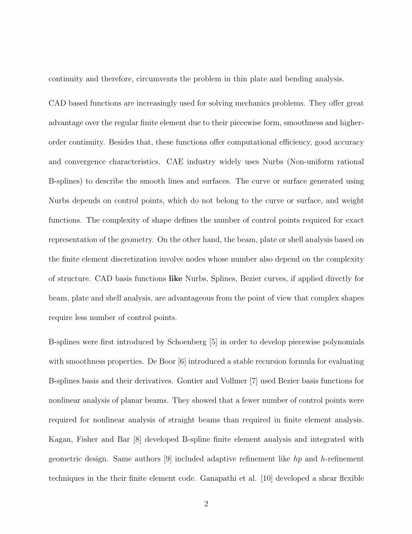
continuity and therefore, circumvents the problem in thin plate and bending analysis.
CAD based functions are increasingly used for solving mechanics problems. They offer great
advantage over the regular finite element due to their piecewise form, smoothness and higher-
order continuity. Besides that, these functions offer computational efficiency, good accuracy
and convergence characteristics. CAE industry widely uses Nurbs (Non-uniform rational
B-splines) to describe the smooth lines and surfaces. The curve or surface generated using
Nurbs depends on control points, which do not belong to the curve or surface, and weight
functions. The complexity of shape defines the number of control points required for exact
representation of the geometry. On the other hand, the beam, plate or shell analysis based on
the finite element discretization involve nodes whose number also depend on the complexity
of structure. CAD basis functions like Nurbs, Splines, Bezier curves, if applied directly for
beam, plate and shell analysis, are advantageous from the point of view that complex shapes
require less number of control points.
B-splines were first introduced by Schoenberg [5] in order to develop piecewise polynomials
with smoothness properties. De Boor [6] introduced a stable recursion formula for evaluating
B-splines basis and their derivatives. Gontier and Vollmer [7] used Bezier basis functions for
nonlinear analysis of planar beams. They showed that a fewer number of control points were
required for nonlinear analysis of straight beams than required in finite element analysis.
Kagan, Fisher and Bar [8] developed B-spline finite element analysis and integrated with
geometric design. Same authors [9] included adaptive refinement like hp and h-refinement
techniques in the their finite element code. Ganapathi et al. [10] developed a shear flexible
2

curved B-spline beam element. They used a field consistency approach (i.e. consistency
of membrane/shear strain fields to obtain the optimal membrane/shear strain functions to
eliminate the shear-locking phenomenon.
1.1.2 Meshless Methods
The finite element method is the most widely used method for solving complex problems. It
offers versatility in solving problems with complex geometries where discretization error can
be reduced by decreasing the element size. However, the lower order polynomial approxi-
mation still leads to inaccuracies in geometric representation and mesh generation results in
higher computational cost. Besides, finite element method has difficulties in solving prob-
lems involving large deformation with severe element distortions, problems involving crack
growth where arbitrary and complex paths do not coincide with the original element inter-
faces and problems involving material fragmentation. And, beam, plate and shell analysis
require higher-order continuity at the inter-element boundary. Therefore, an alternative,
mesh-free approach, seems to be an interesting choice. Meshfree methods are advantageous
from the point of view that they do not require topological generation and provide smooth
approximation over the domain. However, high computational cost of meshfree method is
contributed to the interpolation and numerical integration. Various meshfree methods have
been developed in recent past, namely, reproducing kernel particle method (RKPM)[11],
meshless local Petrov-Galerkin method (MLPG) [12, 13], partition of unity method (PUM)
[14, 15], element-free Galerkin method (EFG) [16, 17, 18], and point interpolation method
3

[19].
1.1.3 Isogeometric Analysis
In-spite of the extensive use of finite element methods, the barriers between engineering
design and analysis still exist and the way to bridge the gap is to reconstitute the entire
process. The geometric approximations in finite element could lead to significant errors and
difficulties, for example, in case of plate with the holes and sharp corners. In order to improve
upon geometry discretization errors is to use Isogeometric analysis approach introduced by
T. J. R. Hughes. There are several CAD functions which can be used for CAD representation
of analysis module. Of most widely used CAD basis in engineering design process are Nurbs
as presented by Piegle and Tiller [20], Farin [21], Cohen et al. [22] and Rogers [23]. Nurbs
represent a billion dollar CAE industry and are useful for analysis purposes because they
possess useful mathematical property of refinement through knot insertion and variational
diminishing property of convex hull. There are other computational geometry technologies
that can be utilized as the basis for Isogeometric analysis such as sub-division surface by
Peters [24] and Warren [25], Gordon patches [26], Greogory patch [27], S-patch [28] and
A-patch [29] etc.
Hughes, Cottrell and Bzilevs [30] introduced the idea of Isogeometric analysis using Nurbs.
They used Nurbs to exactly represent the CAD geometry and then, constructed a coarse
mesh for the analysis. The idea behind Isogeometric analysis is to model the geometry ex-
4

actly which also serves the basis for the solution space i.e. invoking isoparametric concept.
Similarly, Hughes et al. studied structural dynamics and wave propagation [31] and fluid
structure interaction [32] using Isogeometric analysis. Cottrell et al. [33] studied vibra-
tion problem using Isogeometric analysis. Vuong et al. [34] developed a matlab code for
Isogeometric analysis.
1.1.4 Laminated Composite Plate Theories
Advance multi-layered composite and sandwich plate/shell structures are being increasingly
used in aerospace, shipbuilding, bridge and other industries. These structures have smaller
thickness as compared to other dimensions and therefore, are often subjected to large de-
formation behavior under external loads. For accurate prediction of large displacement
behavior, geometric nonlinear analysis is very important and development of computation-
ally efficient geometric nonlinear finite element code for composite plates has been a topic of
considerable interest. The plate theories for laminated composites can be categorized into
equivalent single-layer theories (ELS) and layerwise theories. Equivalent single layer theories
namely, classical, first-order and higher-order shear deformation theories, are derived from
their 3D counterpart (i.e. layerwise and 3D elasticity) by making appropriate assumptions
to the state of strain/stress in the thickness direction, reducing 3D continuum problem to a
2D problem.
Several articles are available in literature on shear deformation theories. Reissner-Mindlin
5
theory [35]-[37] (first-order shear deformation theory) assumes constant state of through
the thickness strain and requires only C0 interpolation functions to satisfy the continuity
requirement. This theory was further extended for anisotropic plates by Whitney and Pagano
[38]. Urthaler and Reddy [39] developed a mixed finite element for bending analysis of
laminated composite plates using FSDT. They treated bending moment as a field variable
along with displacement and rotation.
In higher-order shear deformation theories (HSDT), Putcha and Reddy [40] developed a
mixed finite element approach with 9-node Lagrangian(L) quadrilateral element. Kant and
Kommineni(1992) [41] developed refined HSDT with 9-node quadrilateral(L) element for lin-
ear and nonlinear finite element analysis of laminated composite and sandwich plates. Polit
and Touratier [42] studied large deflection behavior using triangular element. Comparing
higher-order theories and FSDT, higher-order plate theories enhances the accuracy of the
solution slightly but are computationally more expensive, especially for nonlinear analysis
and require C1 continuity. Robbins and Reddy [43] reviewed various ELS and layerwise
theories for laminated composite plates. On the other hand, FSDT has often been used due
to its simplicity and provides best compromise between economy and accuracy in predicting
the response of thin to moderately thick laminates [44]-[45].
6

1.1.5 Shear-Locking and Hourglass Stabilization
During the last few decades, many researchers have made significant contribution to the
development of efficient lower order finite elements based on FSDT. Lower order elements
suffer from shear locking problems as thickness to span ratio becomes too small. Zienkiewicz
et al. [46] and Hughes et al. [47] used reduced or selective integration techniques to solve
the shear locking problem. MacNeal [48], first, developed assumed strain method where
he computed shear strain using kinematic variables at discrete collocation points of the
element other than nodes. Modified versions of this method were successfully proposed by
various researchers such as Bathe and Dvorkin [49], discrete shear elements [50] and linked
interpolation elements by Zienkewicz et al. [51]. Braess, Ming and Shi [52] used enhanced
assumed strain method to counter shear-locking phenomenon.
Discrete Shear Gap (DSG) method improves shear locking behavior by invoking Kirchhoff
constraints on the element nodes. Echter and Bischoff [53] studied locking and unlocking of
Nurbs finite element using discrete shear gap (DSG) method. Zhang and Kim [54] proposed
a locking-free quadrilateral plate element for geometric nonlinear analysis of laminated com-
posite plate. Similarly, Minighini, Tullini and Laudiero [55] developed a locking-free finite
element for shear deformable orthotropic thin-walled beams. Nguyen et al. [56] developed a
smoothed finite element for plate analysis. They incorporated strain smoothing stabilzation
to develop a locking-free plate element. Cai et al. [57] developed a new shear locking-free
triangular plate element with 6 extra degrees of freedom for linear problems. The additional
degrees of freedom account for rotations caused by transverse shear deformation. Their el-
7

ement removed shear locking without extra numerical efforts such as reduced integration,
assumed strain/stress or need for stabilization of zero energy modes.
Shear locking is accompanied with hourglass instability due to reduced integration, thus,
requires stabilization control [58], [59] and [60]. Flanagan and Belytchsko [61] formulated
hourglass control for reduced integration plate element and Tessler and Hughes [62] derived
a plate element which performed well without stabilization. Reddy and Phan [63]’s special
third order theory (STTR) was used for developing displacement based finite element and
similarly, Ren and Hinton [64] developed a third order plate theory but these required C1
continuity for transverse displacement. Codina [65] and Lyly [66] developed a stable first-
order shear deformable plate finite element which was insensitive to mesh distortion.
1.1.6 Interlaminar Stress Calculations
It is a well known fact that composites are prone to damage under low transverse loads
due to comparatively low transverse modulus and have higher probability of failure. The
failure or damage is generally, initiated due to a variety of failure modes like delamination,
matrix cracking, fiber failure etc; delamination being the primary mode of failure. Delamina-
tion is initiated when interlaminar stresses attain maximum interfacial strength. Therefore,
predicting through-the-thickness stresses accurately is essential. This requires calculating
higher-order derivatives of in-plane stresses accurately which in turn requires higher-order
displacement derivatives. Lagrange polynomial start to oscillate as the order of polynomial
8
is increased (Gibbs phenomenon), therefore, are not adequate to calculate transverse stresses
accurately and efficiently.
The first order shear deformation theory with the use of constitutive relation produces highly
inaccurate interlaminar stresses exhibiting non-physical discontinuity at the ply interface of
composite laminate. Accuracy of interlaminar stresses, using 3D equilibrium equations, in
the context of finite element analysis depends upon the computation of higher order in-plane
strain gradients which is generally poor as Lagrange polynomial gradient oscillates. Tessler
[67] developed smoothing variational formulation which combined discrete least square and
penalty constraints functional in a single variational form and recovered the stress gradients
more accurately. Reddy [68] calculated the transverse shear stresses using the derivative
of in-plane stresses that were obtained by differentiating the interpolation functions in fi-
nite element approximation. In order to accurately predict delamination, the interlaminar
normal stress is as important as the shear stress. The computation of interlaminar normal
stress requires an additional derivative of the basis function. These higher-order derivatives
are not obtained directly in the finite element code. Byun and Kapania [69] developed a
post-processing technique to overcome this drawback. They interpolated the finite element
displacement data using polynomial functions like Chebyshev and orthogonal polynomials
in a global domain. Use of Chebyshev polynomials require nodal displacement data to be
available at some specific points i.e. Chebyshev points and can not interpolate the boundary
edge nodal data while orthogonal polynomials use the arbitrarily distributed data points but
are more difficult to obtain. Lee and Lee [70] introduced the non-iterative post processing
9

procedure for the recovery of transverse stresses. They followed the equilibrium based stress
recovery method, using the one dimensional, least square finite element in the thickness
direction.
Park and Kim [71] presented a predictor-corrector post-processing procedure for the accurate
recovery of stresses and displacement in the multi-layered composite panels. The predictor
only predicts the transverse shear stress while the corrector method enhances the accuracy of
the displacement, in-plane and transverse normal stress in the thickness direction using the
results of the predictor and finite element analysis. Park, Park, and Kim [72], later, used the
nonlinear predictor-corrector method to obtain the stresses and displacement in composite
panels in geometrically nonlinear formulation. Noor, Kim, and Peters [73] developed a
computational procedure to get the transverse shear stresses in multi-layered composite
panels. They first used the super convergent recovery technique to evaluate the in-plane
stresses and then, used the piecewise integration in the thickness direction to obtain the
interlaminar stresses.
Matsunaga [74] analyzed the displacement and stresses in laminated beams using global
higher-order beam theory. Author expanded the displacement field variables with power
series of z-coordinate. Makeev and Armanios [75] presented an iterative method to approx-
imate analytical solution of elasticity problems in composite laminates. Rolfes and Rohwer
[76] developed a method for calculating the improved transverse shear stresses in laminated
composites using first-order shear-deformation theory. Kant and Manjunatha [77] developed
numerical algorithms for accurate calculations of transverse stresses using higher-order shear-
10

deformation theories. They used direct integration, finite difference and exact surface fitting
approach. Recently, Kant et al. [78] proposed a semi analytical model for the accurate es-
timation of stresses and displacement in composite and sandwich structures. The two-point
boundary value problem governed by a set of linear first order differential equations through
the thickness is solved using fourth-order Runge-Kutta method. Nosier and Bahrami [79]
developed the analytical solution to study the edge effects in anti-symmetric angle-ply lam-
inates using first order shear deformation and Reddy’s layerwise theory. Senthil and Batra
[80] discussed the analytical solution for thick laminated plates under sinusoidal loads. . [78]
proposed a semi analytical model for the accurate estimation of stresses and displacement
in composite and sandwich structures. The two-point boundary value problem governed by
a set of linear first order differential equations through the thickness is solved using fourth-
order Runge-Kutta method. Nosier and Bahrami [79] developed the analytical solution to
study the edge effects in anti-symmetric angle-ply laminates using first order shear deforma-
tion and Reddy’s layerwise theory. Senthil and Batra [80] discussed the analytical solution
for thick laminated plates under sinusoidal loads.
Stress recovery is highly dependent on the structure of a particular element and on the formu-
lation used in deriving elements. Stress recovery methods include interpolation-extrapolation
from super-convergent points [81], L2 projection [82], stress smoothing [83] and integral
stress techniques [84]. Zienkeiwicz and Zhu [85] developed an efficient post-processing tech-
nique in terms of super-convergent patch recovery (SPR) procedure. A modified version of
this technique was developed to obtain in-plane stresses at nodes and interlaminar stresses
11
using equilibrium equations [86]. Stress recovery procedures suffer from extraneous stress
oscillations [87].
1.1.7 Free Edge Stress Calculations
Developing methods for analysis of composite laminates with curvilinear edges such as cut-
outs is a significantly important research practice. Almost every aircraft structure contains
stress concentration regions such as stiffeners and holes. Rivets and holes are basically
part of structural joints. In laminated composites structures, presence of a hole introduces
significant stress gradients in the vicinity of the hole, in addition to composite being more
susceptible to failure due to low transverse modulus, inhomogeneity, and anisotropy. Many
researchers have studied stress singularity problems in composite plate with a hole using
different techniques such as, boundary layer method [88]-[89], anisotropic elasticity solution
[90], linear finite element method [91], and spline variational method [93], 3D discrete layer
FEM [92]-[94]. Atluri et al. [92] developed a special hole element for prediction of stress
concentration around a hole in composite plate under in-plane load. Iarve [93] used spline
variational three dimensional method for stress analysis in composite plate with open hole.
Raju and Crews [94] performed three dimensional finite element analysis at hole edges in
(0/90)s and (−45/45)s laminates. They used 20-node isoparametric brick element with
highly refined mesh in the vicinity of a hole with approximately 20, 000 dofs. Folias [95]
obtained a local asymptotic solution for three dimensional stress field in the vicinity of free
edge of a hole. Bar-Yoseph and Avrashi [96] developed a sub-structuring approach around
12

the hole to capture the complete stress field. Pan et al. [97] performed stress analysis around
a hole in composite plate under in-plane loading using 3D boundary element method.
1.1.8 Free Vibration and Linear Dynamics
Natural frequency determination play an important role in the design of structures in
aerospace engineering applications. A dynamic study of these structures is essential in as-
sessing their full potential. Vibration characteristics of laminated plates have been studied
extensively in past and finite element method has been used to study vibration problem.
Bert and Mohammad [99],[100] provide extensive literature on modal analysis of laminated
composite plates. Song and Waas [101] conducted free vibration and buckling analysis by
means of higher order beam model. In recent years, mesh-free methods have become an
alternative for vibration analysis including element-free Galerkin method [102], the moving
least square differential quadrature method [103] and the radial basis function method [104].
Liu et al. [105]-[106] proposed a new smoothed finite element method where strain smooth-
ing technique of stabilized conforming nodal integration mesh-free method was incorporated
into existing FEM for 2D elastic problems. Kapania and Raciti [107] did literature survey for
the shear-deformation theories and buckling of laminated composite beams and plates. They
[108], also, reviewed advances in the vibration and wave propagation analysis of laminated
beams and plates.
13

Chapter 2
Interlaminar Stress Calculation in
Composite and Sandwich Beams
This chapter details the development of Nurbs based element-free Galerkin method which
utilizes non-oscillatory nature of higher-order Nurbs basis function and its derivatives to
compute interlaminar normal stress in composite and sandwich beams, accurately and ef-
ficiently. This avoids the extra step in post-processing, generally, required in regular finite
element formulation. Element-free Galerkin formulation is derived for the first order shear
deformable multi-layered composite and sandwich beams. Nurbs basis are derived using
recursion formulation. The displacement and its higher derivatives are computed and com-
pared with the analytical-exact solution. Nurbs formulation used here is also compared with
higher order B-spline basis. It is seen that shear deformable beam developed using Nurbs
basis function is more efficient than the beam developed using older version of B-spline ba-
14

sis. Interlaminar shear and normal stresses are computed directly without the extra step
required in post-processing. Various numerical examples are tested and validated with the
analytical solution.
The chapter is organized as follows. Firstly, the theoretical formulation of Nurbs beam
Galerkin element-free/finite element formulation is derived. Next, transverse/interlaminar
stresses are computed. Code developed is validated with composite and sandwich beams
analysis.
2.1 Theoretical Formulation
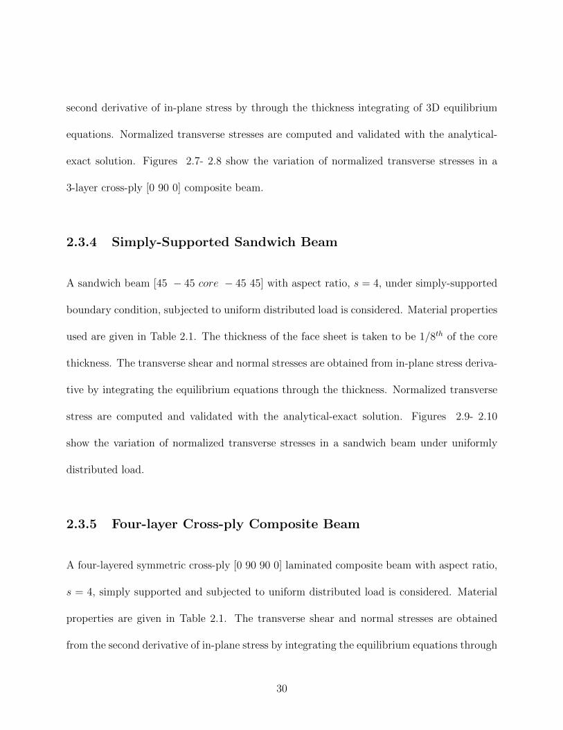
A laminated composite beam consisting of K layers with length L and rectangular cross-
section of width B and depth H is considered here as shown in the Figure 2.1. The
theoretical formulation for the first-order shear-deformable composite beam is obtained by
condensing the first-order shear-deformable plate theory in the y-coordinate. It is assumed
that the width of the laminated plate is small compared to the length and the laminate
scheme, and the loading are such that the displacement is only a function of x-axis.
2.1.1 Displacement and strain field
In the first-order shear-deformation plate theory, the kirchhoff assumption that the transverse
normal remain perpendicular to the mid-surface after deformation is relaxed. And, the
15
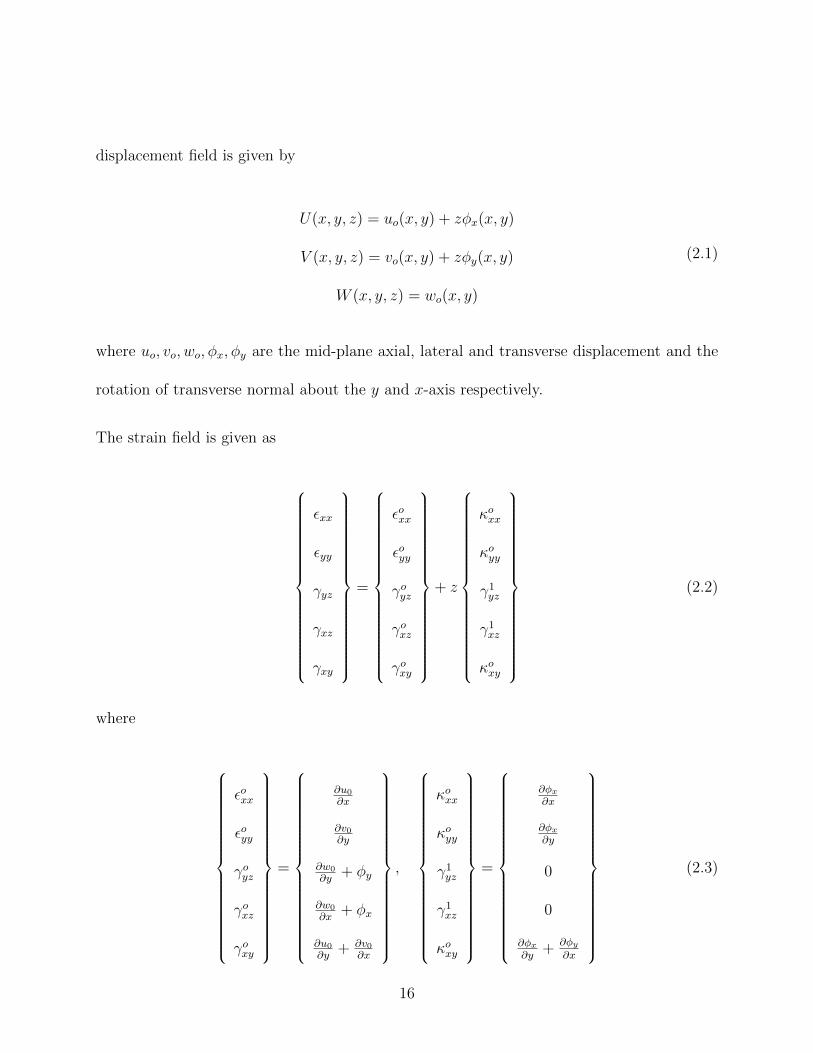
displacement field is given by
U(x, y, z) = uo(x, y) + zφx(x, y)
V (x, y, z) = vo(x, y) + zφy(x, y)
W (x, y, z) = wo(x, y)
(2.1)
where uo, vo, wo, φx, φy are the mid-plane axial, lateral and transverse displacement and the
rotation of transverse normal about the y and x-axis respectively.
The strain field is given as
εxx
εyy
γyz
γxz
γxy
=
εoxx
εoyy
γoyz
γoxz
γoxy
+ z
κoxx
κoyy
γ1yz
γ1xz
κoxy
(2.2)
where
εoxx
εoyy
γoyz
γoxz
γoxy
=
∂u0∂x
∂v0∂y
∂w0
∂y+ φy
∂w0
∂x+ φx
∂u0∂y
+ ∂v0∂x
,
κoxx
κoyy
γ1yz
γ1xz
κoxy
=
∂φx∂x
∂φx∂y
0
0
∂φx∂y
+ ∂φy∂x
(2.3)
16

2.1.2 Constitutive Model
The constitutive relation for the kth lamina in the laminate co-ordinate system can be written
as;
σxx
σxy
σyy
(k)
=
Q11 Q12 Q16
Q12 Q22 Q26
Q16 Q26 Q66
εxx
εyy
εxy
(k)
(2.4)
σyz
σxz
(k)
=
Q44 Q45
Q45 Q55
γyz
γxz
(k)
(2.5)
Where Qijs are the transformed plane-stress reduced stiffnesses.
2.1.3 Laminate Constitutive equations
Laminate constitutive equations for a laminated composite are obtained by integrating the
stresses through the laminate thickness. The resulting force (N ′s) and the moment (M ′s)
resultants are written in the matrix form as given below.
17

Nx
Ny
Nxy
Mx
My
Mxy
=
A11 A12 A16 B11 B12 B16
A12 A22 A26 B12 B22 B26
A16 A26 A66 B16 B26 B66
B11 B12 B16 D11 D12 D16
B12 B22 B26 D12 D22 D26
B16 B26 B66 D16 D26 D66
εox
εoy
γoxy
κox
κoy
κoxy
(2.6)
Qy
Qx
= K
A44 A45
A45 A55
γoyz
γoxz
(2.7)
Here, Aij, Bij and Dij’s are the extensional, bending-extensional and bending stiffness ele-
ments of a laminate.
Symmetric Laminate Composite Beam
Considering bending only problem in a symmetric laminate and negligible bending-extensional
stiffness i.e. [B] = 0, the problem is reduced to pure bending of symmetric laminated beam.
Thus, the inverse form of resulting laminate constitutive equations are written as,
κox
κoy
κoxy
=
D∗11 D∗12 D∗16
D∗12 D∗22 D∗26
D∗16 D∗26 D∗66
Mxx
0
0
(2.8)
18

γoxz
=
1
K
[A∗55
]Qx
(2.9)
where
D∗11 = (D22D66 −D26D26) /D∗
D∗12 = (D16D26 −D12D66) /D∗
D∗16 = (D12D26 −D22D16) /D∗
D∗ = D11D1 +D12D2 +D16D3
D1 = D22D66 −D26D26
D2 = D16D26 −D12D66
D3 = D12D26 −D22D16
(2.10)
A∗44 =A55
A, A∗55 =
A44
A, A∗45 =
A45
A, A = A44A55 − A45A45 (2.11)
D∗ijs denote the elements of the inverse of [D] matrix and A∗ijs denote the elements of inverse
of [A] matrix.
2.1.4 Higher Order Compact B-spline Beam
A B-spline beam consists of m sections with each section of equal length h. The displacement
w and the rotation φ are represented by B-spline basis function and are defined as,
w =m+2∑i=−2
αiϕki , φ =
m+2∑i=−2
βiϕji (2.12)
19
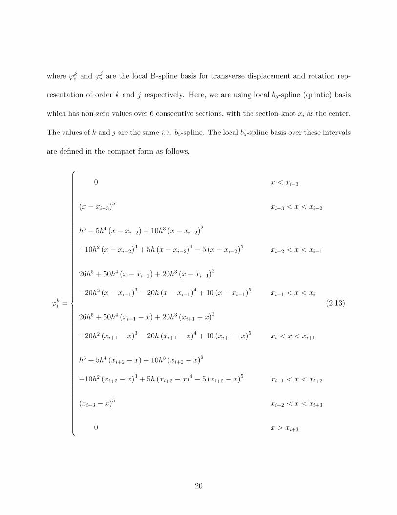
where ϕki and ϕji are the local B-spline basis for transverse displacement and rotation rep-
resentation of order k and j respectively. Here, we are using local b5-spline (quintic) basis
which has non-zero values over 6 consecutive sections, with the section-knot xi as the center.
The values of k and j are the same i.e. b5-spline. The local b5-spline basis over these intervals
are defined in the compact form as follows,
ϕki =
0 x < xi−3
(x− xi−3)5 xi−3 < x < xi−2
h5 + 5h4 (x− xi−2) + 10h3 (x− xi−2)2
+10h2 (x− xi−2)3 + 5h (x− xi−2)4 − 5 (x− xi−2)5 xi−2 < x < xi−1
26h5 + 50h4 (x− xi−1) + 20h3 (x− xi−1)2
−20h2 (x− xi−1)3 − 20h (x− xi−1)4 + 10 (x− xi−1)5 xi−1 < x < xi
26h5 + 50h4 (xi+1 − x) + 20h3 (xi+1 − x)2
−20h2 (xi+1 − x)3 − 20h (xi+1 − x)4 + 10 (xi+1 − x)5 xi < x < xi+1
h5 + 5h4 (xi+2 − x) + 10h3 (xi+2 − x)2
+10h2 (xi+2 − x)3 + 5h (xi+2 − x)4 − 5 (xi+2 − x)5 xi+1 < x < xi+2
(xi+3 − x)5 xi+2 < x < xi+3
0 x > xi+3
(2.13)
20

where αi and βi are the spline parameters. In this formulation, the displacement and rotation
which are present only at the boundaries can be expressed in terms of the spline parameters
as
w0 = (α−2 + 26α−1 + 66α0 + 26α1 + α2)
wm = (αm−2 + 26αm−1 + 66αm + 26αm+1 + αm+2)
w′0 = −5d
(α−2 + 10α−1 − 10α1 − 5α2)
w′m = −5d
(αm−2 + 10αm−1 − 10αm+1 − 5αm+2)
(2.14)
Since, the domain is divided into m sections, there are [2× (m+ 5))] B-spline parame-
ters which represent displacement (w) and rotation (φx) function. The spline parameters
α−2, α−1, αm+1, αm+2 lying outside the domain are replaced by w0, w′0, wm, w
′m and same ap-
plies for the rotation vector. In all, there are [2× (m+ 1))] interior spline parameters within
the domain. This results in an element-free Galerkin formulation i.e. an approximation or
interpolation scheme is constructed entirely from the spline parameters. One of the advan-
tages of meshfree formulation is that it does not require element connectivity.
Gauss-quadrature rule is applied for the numerical integration. In this formulation, the
number of integration points are allowed to vary with the number of spline parameters used
and require testing for the optimal solution.
The generalized vector in terms of physical co-ordinates at the boundary and interior splines,
can be written as
δph = wo w′o αo α1 .............. αm wm w′m (2.15)
21

And, the transformation is obtained using a transformation matrix T as follows,
δph = Tδsp (2.16)
The transformation matrix for the boundary terms consists of coefficients of spline-parameters
given in the equation no. (2.14).
2.1.5 Nurbs Beam Galerkin Formulation
For shear-deformable beam, the displacement fields, w and φ are defined as,
w =CP∑i=1
Rpiwi φ =
CP∑i=1
Rpiφi (2.17)
where Rpi s are the Nurbs basis functions of order p, and CP is the number of control points.
B-spline Basis
A knot vector in one dimension is a set of co-ordinates in the parametric space, written as
Ξ = ξ1, ξ2, ......, ξn+p+1, where ξi is the ith knot, i is the knot index where i = 1, 2, ....., n+
p + 1, p is the order of the polynomial and n is the number of basis functions. The order
of the polynomial, p = 0, 1, 2, 3...., refers to the constant, linear, quadratic, cubic piecewise
polynomials, respectively. The knots in the parametric space are either equally-spaced or
unequally-spaced and the knot vectors are termed as uniform or non-uniform, respectively.
22
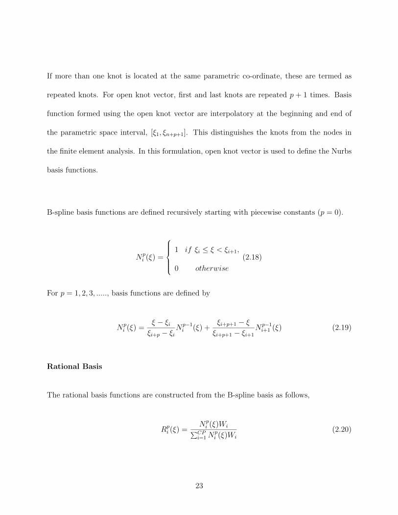
If more than one knot is located at the same parametric co-ordinate, these are termed as
repeated knots. For open knot vector, first and last knots are repeated p + 1 times. Basis
function formed using the open knot vector are interpolatory at the beginning and end of
the parametric space interval, [ξ1, ξn+p+1]. This distinguishes the knots from the nodes in
the finite element analysis. In this formulation, open knot vector is used to define the Nurbs
basis functions.
B-spline basis functions are defined recursively starting with piecewise constants (p = 0).
Npi (ξ) =
1 if ξi ≤ ξ < ξi+1,
0 otherwise
(2.18)
For p = 1, 2, 3, ....., basis functions are defined by
Npi (ξ) =
ξ − ξiξi+p − ξi
Np−1i (ξ) +
ξi+p+1 − ξξi+p+1 − ξi+1
Np−1i+1 (ξ) (2.19)
Rational Basis
The rational basis functions are constructed from the B-spline basis as follows,
Rpi (ξ) =
Npi (ξ)Wi∑CP
i=1Npi (ξ)Wi
(2.20)
23

and, the Nurbs curve can be written as,
C(ξ) =CP∑i=1
Rpi (ξ)Bi (2.21)
where Wis are the weights associated with it. Weights are the vertical coordinate of control
points and Bis are the set of control points.
Some of the important properties of Nurbs are as follows[30] :
1) Nurbs basis functions form a partition of unity.
2) The continuity and support of the Nurbs basis function are the same as those of b-splines.
3) If the weights are equal to 1, Nurbs becomes B-spline.
Figure 2.2 shows the cubic, non-uniform Nurbs basis function for a given knot vector. Nurbs
Basis functions are interpolatory at the end knots, i.e. where the knots are repeated. The
derivation of weak formulation using Galerkin method is given in the appendix A and B.
The refinement process are briefly discussed in the Appendix C.
Substituting the representations for the field variables in the weak formulation, the governing
equation is obtained as follows,
[[Kb] + [Ksh]] δ = F (2.22)
where [Kb] and [Ksh] are the bending and shear stiffness matrices respectively; and F is
24

the consistent load vector.
Kb = EcxxI
0 0
0 K2
(2.23)
Ksh = kshGcxzA
K2 K1T
K1 K0
(2.24)
K0ij =
∫ L0 R
pT
i (x)Rp
j(x)dx
K1ij =
∫ L0 R
pTi (x)R
p′j (x)dx
K2ij =
∫ L0 R
′Ti (x)R
′j(x)dx
F 1i =
∫ L0 R
T
i (x)qdx
(2.25)
The total number of degrees of freedom are equal to d ∗ (m− p− 1), where d is the number
of displacement field variables, m is the length of the knot vector and p is the order of the
polynomial.
This naturally results in element-free Galerkin formulation i.e. an approximation scheme is
constructed entirely from the nodes. Discretization can be performed by increasing the num-
ber of nodes or control points and it is adaptive in nature. Gauss-Quadrature rule is used
for the integration purposes. The number of Gauss points depend on the number of control
points used to discretize the domain and require numerical testing for optimal number of
Gauss-integration points. The boundary conditions are naturally satisfied and required no
additional step.
25
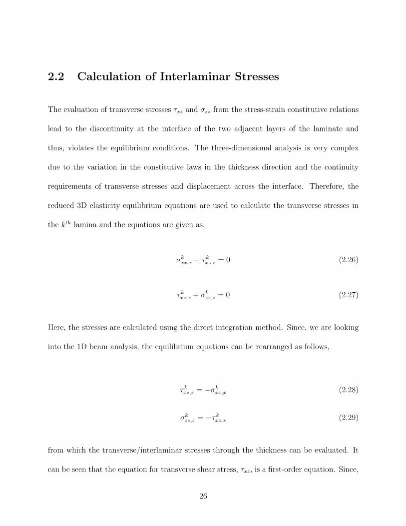
2.2 Calculation of Interlaminar Stresses
The evaluation of transverse stresses τxz and σzz from the stress-strain constitutive relations
lead to the discontinuity at the interface of the two adjacent layers of the laminate and
thus, violates the equilibrium conditions. The three-dimensional analysis is very complex
due to the variation in the constitutive laws in the thickness direction and the continuity
requirements of transverse stresses and displacement across the interface. Therefore, the
reduced 3D elasticity equilibrium equations are used to calculate the transverse stresses in
the kth lamina and the equations are given as,
σkxx,x + τ kxz,z = 0 (2.26)
τ kxz,x + σkzz,z = 0 (2.27)
Here, the stresses are calculated using the direct integration method. Since, we are looking
into the 1D beam analysis, the equilibrium equations can be rearranged as follows,
τ kxz,z = −σkxx,x (2.28)
σkzz,z = −τ kxz,x (2.29)
from which the transverse/interlaminar stresses through the thickness can be evaluated. It
can be seen that the equation for transverse shear stress, τxz, is a first-order equation. Since,
26

in general, the transverse shear stresses are known at the top and bottom of the laminate, one
can only obtain a non-unique solution as both the traction boundary conditions can not be
enforced simultaneously. However, for the transverse normal stresses, a second-order equa-
tion is derived and requires double integration through the thickness. Two constants can be
evaluated from the traction boundary conditions at the top and bottom of the laminate[77].
The 3D equilibrium equations for transverse stress calculations are as follows,
τ kxz =∫ zi+1
zi
(σkxx,x
)dz +Hk(x) (2.30)
σkzz|k+1 =k∑i=1
∫ zi+1
zi
(∫zσxx,xx dz
)dz + zG1 +G2 (2.31)
where Hk, G1 and G2 are the constants of integration.
2.3 Numerical Examples
In this section, numerical examples of composite and sandwich beam under transverse uni-
formly distributed load for different boundary conditions are presented. The higher-order
derivatives and transverse stresses are calculated for different cases and compared with the
analytical exact solution. The material properties used here are given in Table 1.1. The
transverse stresses calculated for various numerical examples are normalized using the fol-
lowing notation.
27
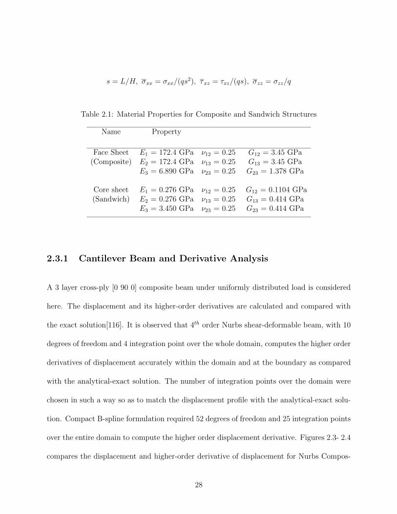
s = L/H, σxx = σxx/(qs2), τxz = τxz/(qs), σzz = σzz/q
Table 2.1: Material Properties for Composite and Sandwich Structures
Name Property
Face Sheet E1 = 172.4 GPa ν12 = 0.25 G12 = 3.45 GPa(Composite) E2 = 172.4 GPa ν13 = 0.25 G13 = 3.45 GPa
E3 = 6.890 GPa ν23 = 0.25 G23 = 1.378 GPa
Core sheet E1 = 0.276 GPa ν12 = 0.25 G12 = 0.1104 GPa(Sandwich) E2 = 0.276 GPa ν13 = 0.25 G13 = 0.414 GPa
E3 = 3.450 GPa ν23 = 0.25 G23 = 0.414 GPa
2.3.1 Cantilever Beam and Derivative Analysis
A 3 layer cross-ply [0 90 0] composite beam under uniformly distributed load is considered
here. The displacement and its higher-order derivatives are calculated and compared with
the exact solution[116]. It is observed that 4th order Nurbs shear-deformable beam, with 10
degrees of freedom and 4 integration point over the whole domain, computes the higher order
derivatives of displacement accurately within the domain and at the boundary as compared
with the analytical-exact solution. The number of integration points over the domain were
chosen in such a way so as to match the displacement profile with the analytical-exact solu-
tion. Compact B-spline formulation required 52 degrees of freedom and 25 integration points
over the entire domain to compute the higher order displacement derivative. Figures 2.3- 2.4
compares the displacement and higher-order derivative of displacement for Nurbs Compos-
28

ite beam with the analytical-exact solution and higher order compact B-spline(HOCBS)
formulation.
2.3.2 Simply-Supported Beam and Derivative Analysis
A 3 layer cross-ply [0900] composite beam under uniformly distributed load is considered.
The displacement and its derivatives are compared with the closed form / analytical exact
solution and compact B-spline formulation. It is observed that the 4th order Nurbs basis, with
10 degrees of freedom and 5 integration point over the whole domain, computes higher order
derivatives of displacement accurately within the domain and at the boundary as compared
with the analytical-exact solution. B-spline formulation again required more number of
B-spline parameters and integration points i.e. 50 degrees of freedom with 24 integration
points were required for the same analysis. Figures 2.5- 2.6 compares the displacement and
its higher-order derivatives for Nurbs basis as compared with the analytical-exact solution
and higher order compact B-spline (HOBS) formulation.
2.3.3 Simply-Supported Cross-ply Beam
A three-layered cross-ply [0 90 0], simply supported, laminated composite beam with aspect
ratio, s = 4 under uniformly distributed load is considered. Nurbs based shear-deformable
beam formulation is used for the computation of interlaminar stress. Material properties
are given in Table 2.1. The transverse shear and normal stresses are computed from the
29
second derivative of in-plane stress by through the thickness integrating of 3D equilibrium
equations. Normalized transverse stresses are computed and validated with the analytical-
exact solution. Figures 2.7- 2.8 show the variation of normalized transverse stresses in a
3-layer cross-ply [0 90 0] composite beam.
2.3.4 Simply-Supported Sandwich Beam
A sandwich beam [45 − 45 core − 45 45] with aspect ratio, s = 4, under simply-supported
boundary condition, subjected to uniform distributed load is considered. Material properties
used are given in Table 2.1. The thickness of the face sheet is taken to be 1/8th of the core
thickness. The transverse shear and normal stresses are obtained from in-plane stress deriva-
tive by integrating the equilibrium equations through the thickness. Normalized transverse
stress are computed and validated with the analytical-exact solution. Figures 2.9- 2.10
show the variation of normalized transverse stresses in a sandwich beam under uniformly
distributed load.
2.3.5 Four-layer Cross-ply Composite Beam
A four-layered symmetric cross-ply [0 90 90 0] laminated composite beam with aspect ratio,
s = 4, simply supported and subjected to uniform distributed load is considered. Material
properties are given in Table 2.1. The transverse shear and normal stresses are obtained
from the second derivative of in-plane stress by integrating the equilibrium equations through
30

the thickness. Normalized transverse stress results are validated with the analytical-exact
solution[116]. Figures 2.11- 2.12 show the variation of normalized transverse stresses in a
four-layer cross-ply laminated composite beam.
2.4 Conclusion
A variable-order Nurbs shear-deformable laminated composite element-free beam formula-
tion is developed. The displacement and interlaminar stresses are computed for composite
and sandwich beams under transverse loads. Nurbs beam required less number of control
points to obtain the higher order derivatives of displacement and is found to be more ef-
ficient than the B-spline formulation. The higher-order derivative required for computing
transverse/interlaminar normal stress is obtained directly i.e. without using an extra step in
post-processing, necessitated in the finite element formulation. This is attributed to higher
order continuity and smoothness properties of Nurbs basis due to stable recursion algorithm.
The present computational analysis is more rigorous as the loading is uniformly distributed
over the domain of the beam. Higher-order displacement derivatives and interlaminar stresses
are accurately and efficiently computed and compared with the closed-form solution.
31
2.5 Appendix
2.5.1 Governing Equations
The special case of principle of virtual displacement that deals with linear as well as non-
linear elastic bodies is known as principle of minimum total potential energy. The principle
of minimum total potential energy is used to derive the governing equations for first-order
shear deformable composite beam. The principle states that under equilibrium conditions,
the first variation of the total potential energy i.e. the sum of the strain energy and the
potential of the applied loads is zero i.e.
δ (U + V ) = δU + δV = 0 (2.32)
δU =∫ L
0
∫A
[σxx δεxx + σxzδγxz] dAdx (2.33)
δV = −∫ L
0q δw0 dx (2.34)
where q is the distributed load at the top surface (z = −h/2) of the laminate. Integrating
over the area, ∫ L
0
(Mxxδε
1xx +Qxδγ
0xz − qδw0
)dx = 0 (2.35)
Integrating over the parts,
∫ L
0(−Mxx,x +Qx) δφ+ (−q −Qx,x) δwo dx+ Mxxδφ+Qxδwo |L0 = 0 (2.36)
32

Thus, the Euler-Lagrange equations are,
δwo : Qx,x + q = 0 (2.37)
δφ : Mxx,x −Qx = 0 (2.38)
Where, wo and φ are the primary variables and Mxx and Qx are the secondary variables.
The governing equation of motion in terms of displacement variables can be written as,
kshGcxzA
(∂2wo∂x2
+∂φx∂x
)+ q = 0 (2.39)
EcxxIyy
∂2φx∂x2
− kshGcxzA
(∂wo∂x
+ φx
)= 0 (2.40)
where, EcxxIyy = 12
D∗11H3 , G
cxzA = 1
A∗55Hare the equivalent moduli for the composite beam,
A = BH, is the area of cross-section and ksh is the shear-correction factor.
2.5.2 Weighted Residual-Galerkin Method
The weak formulation for the strong form of governing equations is derived by using the
weighted residual-Galerkin method. Here, -w1 and -w2 are the weight functions which reduce
the order of the equations resulting in a weak formulation. Multiplying equations (34) & (35)
with weight functions and integrating over the element domain Ωe, we obtain the following
form, ∫ xB
xA−w1 kshGc
xzA (wo,xx + φx,x) + q = 0 (2.41)
33

∫ xB
xA−w2 [Ec
xxIyyφx,xx − kshGcxzA (wo,x + φx)] = 0 (2.42)
Integrating by parts once, we obtain
∫ xB
xA[w1,x kshGc
xzA (wo,x + φx) − w1q] dx− w1(xA)Qe1 (2.43)
−w1(xB)Qe3 = 0∫ xB
xA[w2,x (Ec
xxIyyφx,x) + w2kshGcxzA (w,x + φx)] dx− w2(xA)Qe
2 (2.44)
−w2(xB)Qe4 = 0
(2.45)
where
Qe1 = − [kshG
cxzA (φx + w,x)] |xA , Qe
3 = [kshGcxzA (φx + w,x)] |xB (2.46)
Qe2 = − (Ec
xxφx,x) |xA , Qe4 = (Ec
xxφx,x) |xB (2.47)
For the Galerkin method, wi = ϕi i.e. weight/trial functions are replaced by the same basis
function as used to define the displacement and rotation fields. In our case, xA = 0, xB = L.
34
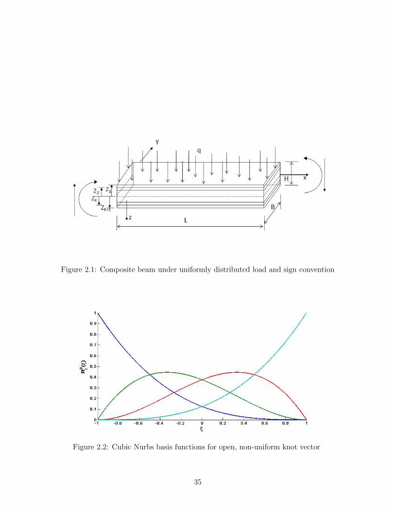
Figure 2.1: Composite beam under uniformly distributed load and sign convention
Figure 2.2: Cubic Nurbs basis functions for open, non-uniform knot vector
35
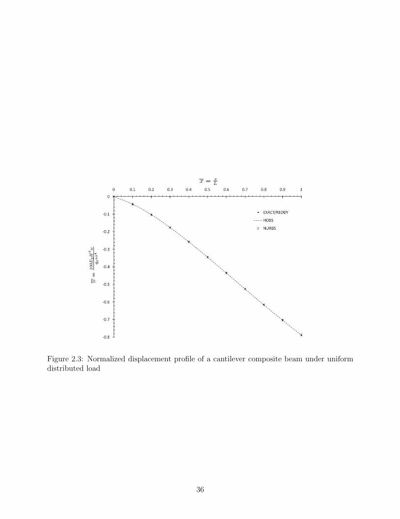
Figure 2.3: Normalized displacement profile of a cantilever composite beam under uniformdistributed load
36

Figure 2.4: Normalized second derivative of displacement of a cantilever composite beamunder uniform distributed load
37

Figure 2.5: Normalized displacement profile over the length of a simply supported compositebeam under uniform distributed load
38

Figure 2.6: Normalized second derivative of displacement of a simply supported compositebeam under uniform distributed load
39

Figure 2.7: Variation of normalized transverse shear stress through the thickness in a cross-ply [0 90 0] laminate composite beam under uniform distributed load
40

Figure 2.8: Variation of normalized transverse normal stress through the thickness in across-ply [0 90 0] laminate composite beam under uniform distributed load
41

Figure 2.9: Variation of normalized transverse shear stress through the thickness in a sand-wich beam [45 -45 core -45 45] under uniform distributed load
42

Figure 2.10: Variation of normalized transverse normal stress in a sandwich beam [45 -45core -45 45] under uniform distributed load
43
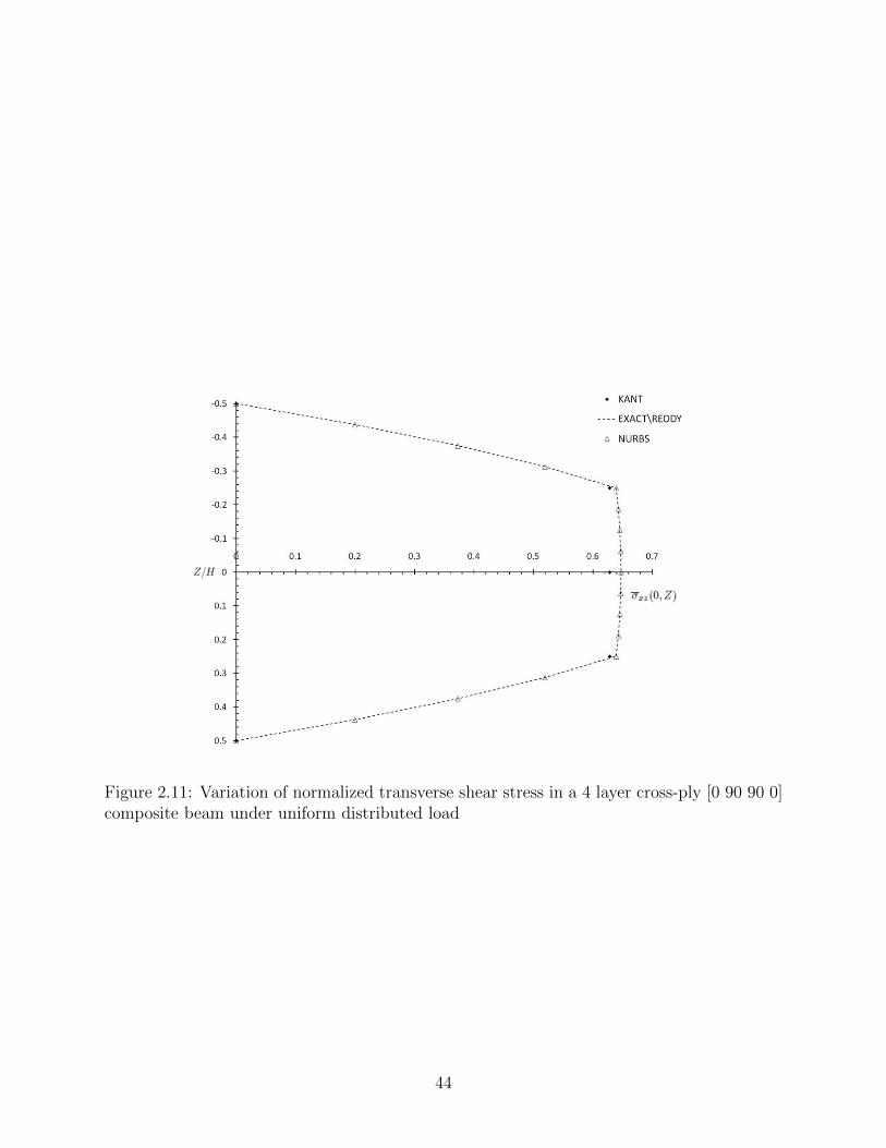
Figure 2.11: Variation of normalized transverse shear stress in a 4 layer cross-ply [0 90 90 0]composite beam under uniform distributed load
44

Figure 2.12: Variation of normalized transverse normal stress in a 4 layer cross-ply [0 90 900] composite beam under uniform distributed load
45

Chapter 3
Geometrically Nonlinear Nurbs
Isogeometric Finite Element Analysis
of Laminated Composite Plate
This research present the development of geometrically nonlinear Nurbs Isogeometric fi-
nite element analysis of laminated composite plates. First-order, shear-deformable laminate
composite plate theory is utilized in deriving the governing equations using a variational for-
mulation. Geometric nonlinearity is accounted for in Von-Karman sense. Nurbs quadratic
and higher-order elements are constructed where k-refinement has no analogous in regular
finite element. Isotropic, orthotropic and laminated composite plates are studied for vari-
ous boundary conditions, length to thickness ratios and ply-angles. The computed center
46

direction is found to be in an excellent agreement with the literature and required fewer
degrees of freedom/control point when compared with regular finite element analysis. For
thin plate analysis, k-refined, quadratic Nurbs element is found to remedy the shear lock-
ing problem, i.e. it eliminated the need for reduced integration of transverse shear stifiness
terms. k-refined quadratic Nurbs element also provided stable nonlinear deflection (hour-
glass instability) for distorted quadrilateral meshes. This research presents the development
of Nurbs Isogeometric finite element where k-refined Nurbs element eliminates the need for
extra step required in developing locking-free and stable shear-deformable plate elements.
3.1 Theoretical Formulation
3.1.1 First-order shear deformation plate theory (FSDT)
Displacement and strain field
The origin of the material coordinate system is considered to be the mid-plane of the laminate
and the Kirchhoff assumption, that the transverse normal remain perpendicular to the mid-
surface after deformation, is relaxed. Figure 3.1shows the coordinate system and layer
numbering of a laminated composite plate. The displacement field is defined as,
u(x, y, z) = u0(x, y) + zφx(x, y)
47

v(x, y, z) = v0(x, y) + zφy(x, y) (3.1)
w(x, y, z) = w0(x, y)
where u0, v0, w0 are the displacement along the x, y and z-axis and φx, φy are the rotation of
transverse normal of the mid-plane about the y and x-axis respectively. Figure 3.2 shows the
undeformed and deformed configuration of first order shear-deformable laminated composite
plate.
x
yz
kh/2
h/2
Figure 3.1: Coordinate system and layer numbering used for a laminate plate
The strain vector is obtained in terms of Green-Lagrange strain and accounts for large trans-
verse displacement, small strain and moderate rotation. The strain vector corresponding to
48
the displacement field is given as,
εxx =∂u
∂x+
1
2
(∂w
∂x
)2
εyy =∂v
∂y+
1
2
(∂w
∂y
)2
γyz =∂w
∂y+ φy (3.2)
γxz =∂w
∂x+ φx
γxy =∂u
∂y+∂v
∂x+∂w
∂x
∂w
∂y
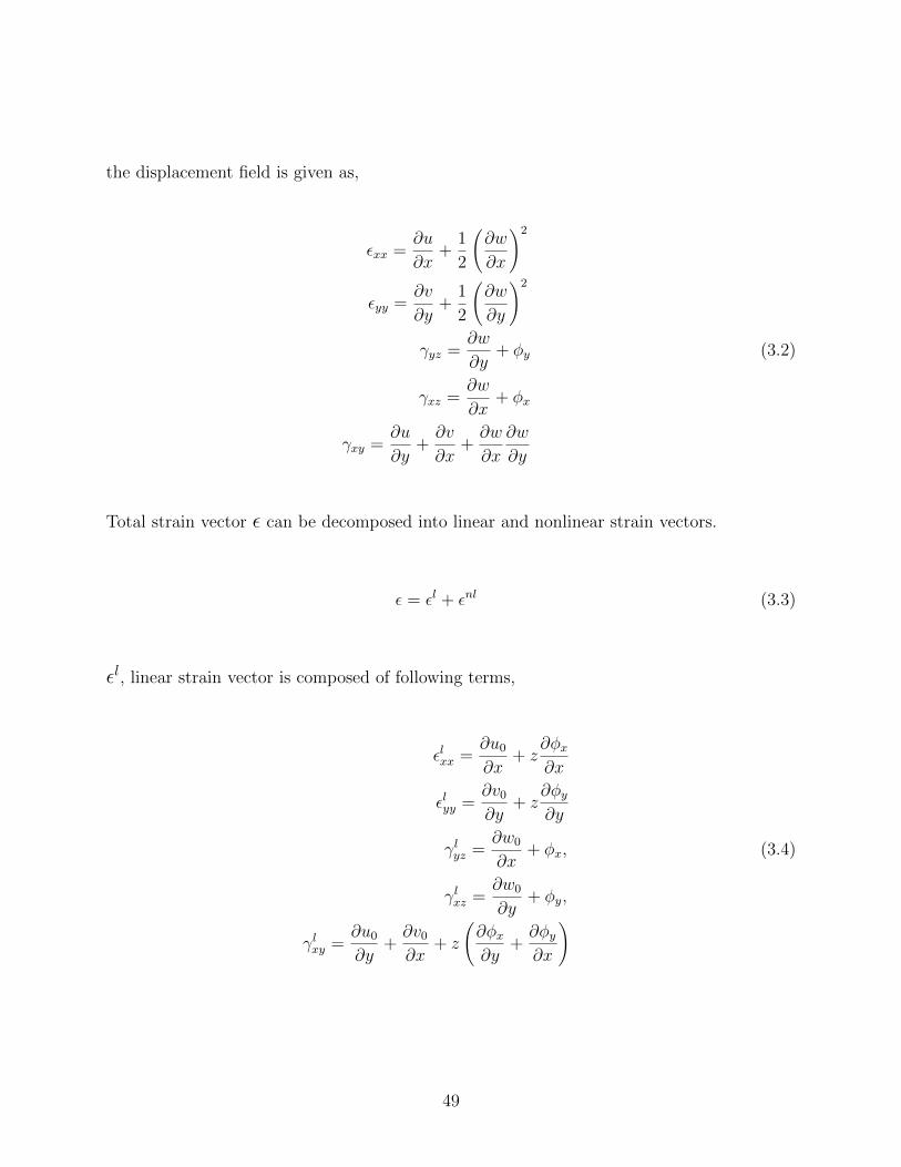
Total strain vector ε can be decomposed into linear and nonlinear strain vectors.
ε = εl + εnl (3.3)
εl, linear strain vector is composed of following terms,
εlxx =∂u0
∂x+ z
∂φx∂x
εlyy =∂v0
∂y+ z
∂φy∂y
γlyz =∂w0
∂x+ φx, (3.4)
γlxz =∂w0
∂y+ φy,
γlxy =∂u0
∂y+∂v0
∂x+ z
(∂φx∂y
+∂φy∂x
)
49

εnl, the nonlinear strain vector contains the following terms,
εnlxx =1
2
(∂w0
∂x
)2
εnlyy =1
2
(∂w0
∂y
)2
(3.5)
γnlxy =∂w0
∂x
∂w0
∂y
Other higher order terms are considered to be negeligible.
Figure 3.2: Undeformed and deformed configuration of first order shear-deformable plate
50
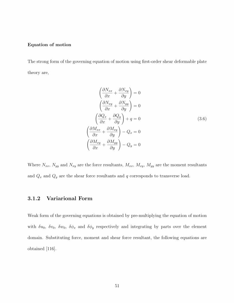
Equation of motion
The strong form of the governing equation of motion using first-order shear deformable plate
theory are,
(∂Nxx
∂x+∂Nxy
∂y
)= 0(
∂Nxy
∂x+∂Nyy
∂y
)= 0(
∂Qx
∂x+∂Qy
∂y
)+ q = 0 (3.6)(
∂Mxx
∂x+∂Mxy
∂y
)−Qx = 0(
∂Mxy
∂x+∂Myy
∂y
)−Qy = 0
Where Nxx, Nyy and Nxy are the force resultants, Mxx, Mxy, Myy are the moment resultants
and Qx and Qy are the shear force resultants and q corresponds to transverse load.
3.1.2 Variarional Form
Weak form of the governing equations is obtained by pre-multiplying the equation of motion
with δu0, δv0, δw0, δφx and δφy respectively and integrating by parts over the element
domain. Substituting force, moment and shear force resultant, the following equations are
obtained [116].
51

0 =∫
Ωe
∂δu0
∂x
A11
∂u0
∂x+
1
2
(∂w0
∂x
)2+ A12
∂v0
∂y+
1
2
(∂w0
∂y
)2
+A16
(∂u0
∂y+∂v0
∂x+∂w0
∂x
∂w0
∂y
)+B11
∂φx∂x
+B12∂φy∂y
+B16
(∂φx∂y
+∂φy∂x
)
+∂δu0
∂y
A16
∂u0
∂x+
1
2
(∂w0
∂x
)2+ A26
∂v0
∂y+
1
2
(∂w0
∂y
)2
+A66
(∂u0
∂y+∂v0
∂x+∂w0
∂x
∂w0
∂y
)+B16
∂φx∂x
+B26∂φy∂y
+B66
(∂φx∂y
+∂φy∂x
)]dxdy
−∮
ΓeNnδu0nds (3.7)
0 =∫
Ωe
∂δv0
∂x
A12
∂u0
∂x+
1
2
(∂w0
∂x
)2+ A22
∂v0
∂y+
1
2
(∂w0
∂y
)2
+A26
(∂u0
∂y+∂v0
∂x+∂w0
∂x
∂w0
∂y
)+B12
φxx
+B22φy∂y
+B26
(φx∂y
+φy∂x
)
+∂δv0
∂x
A16
∂u0
∂x+
1
2
(∂w0
∂x
)2+ A26
∂v0
∂y+
1
2
(∂w0
∂y
)2
+A66
(∂u0
∂y+∂v0
∂x+∂w0
∂x
∂w0
∂y
)+B16
∂φx∂x
+B26∂φy∂y
+B66
(∂φx∂y
+∂φy∂x
)]dxdy −
∮ΓeNsδv0sds (3.8)
0 = Ks
∫Ωe
[∂δw0
∂x
A55
(∂w0
∂x+ φx
)+ A45
(∂w0
∂y+ φy
)
52
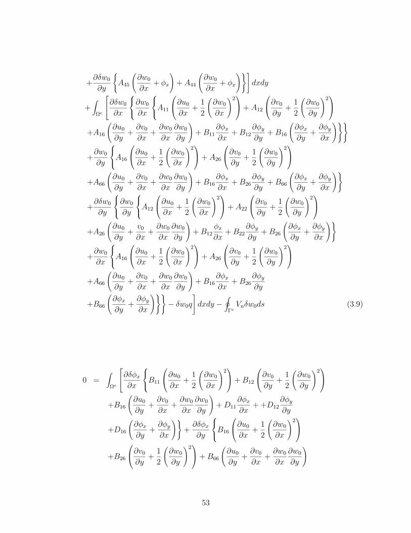
+∂δw0
∂y
A45
(∂w0
∂x+ φx
)+ A44
(∂w0
∂x+ φx
)]dxdy
+∫
Ωe
∂δw0
∂x
∂w0
∂x
A11
∂u0
∂x+
1
2
(∂w0
∂x
)2+ A12
∂v0
∂y+
1
2
(∂w0
∂y
)2
+A16
(∂u0
∂y+∂v0
∂x+∂w0
∂x
∂w0
∂y
)+B11
∂φx∂x
+B12∂φy∂y
+B16
(∂φx∂y
+∂φy∂x
)
+∂w0
∂y
A16
∂u0
∂x+
1
2
(∂w0
∂x
)2+ A26
∂v0
∂y+
1
2
(∂w0
∂y
)2
+A66
(∂u0
∂y+∂v0
∂x+∂w0
∂x
∂w0
∂y
)+B16
∂φx∂x
+B26∂φy∂y
+B66
(∂φx∂y
+∂φy∂x
)
+∂δw0
∂y
∂w0
∂y
A12
∂u0
∂x+
1
2
(∂w0
∂x
)2+ A22
∂v0
∂y+
1
2
(∂w0
∂y
)2
+A26
(∂u0
∂y+v0
∂x+∂w0
∂x
∂w0
∂y
)+B12
φx∂x
+B22∂φy∂y
+B26
(∂φx∂y
+∂φy∂x
)
+∂w0
∂x
A16
∂u0
∂x+
1
2
(∂w0
∂x
)2+ A26
∂v0
∂y+
1
2
(∂w0
∂y
)2
+A66
(∂u0
∂y+∂v0
∂x+∂w0
∂x
∂w0
∂y
)+B16
∂φx∂x
+B26∂φy∂y
+B66
(∂φx∂y
+∂φy∂x
)− δw0q
]dxdy −
∮ΓeVnδw0ds (3.9)
0 =∫
Ωe
∂δφx∂x
B11
∂u0
∂x+
1
2
(∂w0
∂x
)2+B12
∂v0
∂y+
1
2
(∂w0
∂y
)2
+B16
(∂u0
∂y+∂v0
∂x+∂w0
∂x
∂w0
∂y
)+D11
∂φx∂x
+ +D12∂φy∂y
+D16
(∂φx∂y
+∂φy∂x
)+∂δφx∂y
B16
∂u0
∂x+
1
2
(∂w0
∂x
)2
+B26
∂v0
∂y+
1
2
(∂w0
∂y
)2+B66
(∂u0
∂y+∂v0
∂x+∂w0
∂x
∂w0
∂y
)
53

+D16∂φx∂x
+D26∂φy∂y
+D66
(∂φx∂y
+∂φy∂x
)
+Ksδφx
(A55
(φx +
∂w0
∂x
)+ A45
(φy +
∂w0
∂y
))]dxdy
−∮
ΓeMnδφnds (3.10)
0 =∫
Ωe
∂δφy∂y
B12
∂v0
∂y+
1
2
(∂w0
∂y
)2+B22
∂v0
∂y+
1
2
(∂w0
∂y
)2
+B26
(∂u0
∂y+∂v0
∂x+∂w0
∂x
∂w0
∂y
)+D12
∂φx∂x
+D22∂φy∂y
+D26
(∂φx∂y
+∂φy∂x
)+∂δφy∂x
B16
∂u0
∂x+
1
2
(∂w0
∂x
)2
+B26
∂v0
∂y+
1
2
(∂w0
∂y
)2+B66
(∂u0
∂y+∂v0
∂x+∂w0
∂x
∂w0
∂y
)
. +D16∂φx∂x
+D26∂φy∂y
+D66
(∂φx∂y
+∂φy∂x
)
+Ksδφy
A45
(φx +
∂w0
∂x
)+ A44
(φy +
∂w0
∂y
)]dxdy
−∮
ΓeMsδφsds (3.11)
And, the secondary variables are given as,
Nn = Nxxnx +Nxyny, Ns = Nxynx +Nyyny
Mn = Mxxnx +Mxyny, Ms = Mxynx +Myyny (3.12)
Vn =
(Qx +Nxx
∂w0
∂x+Nxy
∂w0
∂y
)nx +
(Qy +Nxy
∂w0
∂x+Nyy
∂w0
∂y
)ny
54

The laminate constitutive equations relate the force and moment resultant to strains in
laminate coordinate system through ABD matrix.
Nxx
Nyy
Nxy
=
A11 A12 A16
A12 A22 A26
A16 A26 A66
∂u0∂x
+ 12
(∂w0
∂x
)2
∂v0∂y
+ 12
(∂w0
∂y
)2
∂u0∂y
+ ∂v0∂x
+(∂w0
∂x∂w0
∂y
)
+
B11 B12 B16
B12 B22 B26
B16 B26 B66
∂φx∂x
∂φy∂y
∂φx∂y
+ ∂phiy∂x
(3.13)
Mxx
Myy
Mxy
=
B11 B12 B16
B12 B22 B26
B16 B26 B66
∂u0∂x
+ 12
(∂w0
∂x
)2
∂v0∂y
+ 12
(∂w0
∂y
)2
∂u0∂y
+ ∂v0∂x
+(∂w0
∂x∂w0
∂y
)
+
D11 D12 D16
D12 D22 D26
D16 D26 D66
∂φx∂x
∂φy∂y
∂φx∂y
+ ∂φy∂x
(3.14)
Qy
Qx
= K
A44 A45
A45 A55
∂w0
∂y+ φy
∂w0
∂y+ φy
(3.15)
55

(Aij, Bij, Dij) =N∑k=1
(Qk
ij (zk+1 − zk) ,1
2Qk
ij
(z2k+1 − z2
k
),1
3Qk
ij
(z3k+1 − z3
k
))
(A44, A45, A55) =N∑k=1
(Qk44, Q
k45, Q
k55
)(zk+1 − zk) (3.16)
In ABD matrix, Aij, Bij and Dij represent extensional and shear, extensional-bending cou-
pling and bending stiffness terms and Qkijs are plane-stress reduced stiffness terms.
3.2 Geometrically Nonlinear Nurbs Isogeometric Fi-
nite Element Formulation
3.2.1 Displacement field approximation
The dependent displacement field variables are approximated by Nurbs basis as follows,
u0(x, y) =nCP∑j=1
ujRj(x(ξ, η), y(ξ, η)), v0(x, y) =nCP∑j=1
vjRj(x(ξ, η), y(ξ, η))
w0(x, y) =nCP∑j=1
wjRj(x(ξ, η), y(ξ, η)) (3.17)
56

φx(x, y) =nCP∑j=1
φxjRj(x(ξ, η), y(ξ, η)), φy(x, y) =nCP∑j=1
φyjRj(x(ξ, η), y(ξ, η))
where nCP are the number of control points per element and Rj are 2D Nurbs basis.
3.2.2 Nurbs Basis
In this section, h, p and k-refined Nurbs elements are derived. This subsection details the
step by step B-spline and rational basis generation and describes the transformation from
physical to parametric to parent domain using schematic iustration. h, p and k-refinement
elements are constructed by different ways of modifying the knot vector by knot-insertion.
Last part of this subsection describes the construction of various elements.
B-spline Basis
A knot vector in one dimension is a set of co-ordinates in the parametric space,
Ξ = ξ1, ξ2, ......, ξn+p+1, where ξi is the ith knot, i is the knot index where i = 1, 2, ....., n+
p + 1, p is the order of the polynomial and n is the number of basis functions. The order
of the polynomial, p = 0, 1, 2, 3...., refer to the constant, linear, quadratic, cubic piecewise
polynomials, respectively. If more than one knot is located at the same parametric co-
ordinate, these are termed as repeated knots. In case of open knot vector, first and last knots
are repeated p+ 1 times. Basis functions formed using open knot vector are interpolatory at
the beginning and end of the parametric space interval, i.e. [ξ1, ξn+p+1]. This distinguishes
57

the knots from the nodes in the finite element analysis as all the nodes are interpolatory. As a
starting point, B-spline basis functions are defined recursively using Cox-Deboor algorithm,
starting with piecewise constants (p = 0).
Npi (ξ) =
1 if ξi ≤ ξ < ξi+1,
0 otherwise
(3.18)
And, subsequently, basis functions for orders p = 1, 2, 3, ....., are defined as follows,
Npi (ξ) =
ξ − ξiξi+p − ξi
Np−1i (ξ) +
ξi+p+1 − ξξi+p+1 − ξi+1
Np−1i+1 (ξ) (3.19)
Rational B-spline (Nurbs) Basis
Nurbs basis are formed by a tensor product of B-spline basis in ξ and η direction and using
projective weights associated with the control points. Rational basis are very similar to
B-spline basis and derive the continuity and support for the functional from the knot vector.
Also, Nurbs basis form a partition of unity and are pointwise non-negetive. These properties
result in a strong convex hull property. Rational basis are formed as follows,
Rp,qi,j (ξ, η) =
Npi (ξ)M q
j (η)Wi,j∑CPwi=1
∑CPui=1 Np
i (ξ)M qj (η)Wi,j
≈ Rpk k = 1 : nCP (3.20)
58
Nurbs surface is defined as,
S(x, y) =CPw∑j=1
CPu∑i=1
Rp,qi,j (ξ, η)Bi,j (3.21)
where Npi (ξ) and M q
j (η) are the B-spline basis in ξ and η direction and Rp,qi,j denotes a 2D
Nurbs basis function. CPw and CPu are the number of control points in ξ and η directions
and nCP = CPu × CPw is the total number of control points per element. Wi,js are the
weights associated with the control points, Bi,j and weights are the vertical coordinates of
the corresponding control points. Here, weights are equal to one resulting in specialized
form.
3.2.3 Numerical Integration
A multi-element patch, a tensor product of knot vectors in ξ and η directions, i.e. 0 0 0.5 1 1×
0 0 0.5 1 1, creates a 2× 2 plate mesh in physical domain. Nurbs basis multiplied with
respective control points constructs a geometric model of plate.
In order to perform numerical integration, Guass quadrature is employed. The integration
on physical domain is performed by transformation from physical to parametric to parent
domain and is performed over the index space. Index space is the space of a tensor product
of knot vectors in ξ and η directions. The mapping between physical and parametric domain
59

is performed as follows,
x
y
=nCP∑k=1
R1k(ξ, η)
Bxk
Byk
∂Rpk
∂x
∂Rpk
∂y
= [J−1]
∂Rp
k(ξ,η)∂ξ
∂Rpk(ξ,η)∂η
[J ] =
∂x∂ξ
∂y∂ξ
∂x∂η
∂y∂η
(3.22)
Bxk and Byk are control point coordinates and Jxξyη is the mapping from physical to para-
metric domain. Mapping from parametric to parent domain is the standard mapping as is
done in finite element. Figure 6.3 shows schematic of Isogeometric framework.
3.2.4 Nurbs Elements
Various lower and higher order Nurbs elements can be constructed by utilizing various ele-
ment k-refinement techniques. 9LinNurbsKR1,2/F (k-refined, 9 control point/element, lin-
ear Nurbs element with knot insertion at location 0.25 and 0 in knot vector respectively),
9QuadNurbs/(F/R) element with 9 control point/element, 16CubicNurbs/(F/R) and (k-
refined) 16QuadNurbsKR/F with 16 control point/element and 25QuarticNurbs, 25Cubic-
60
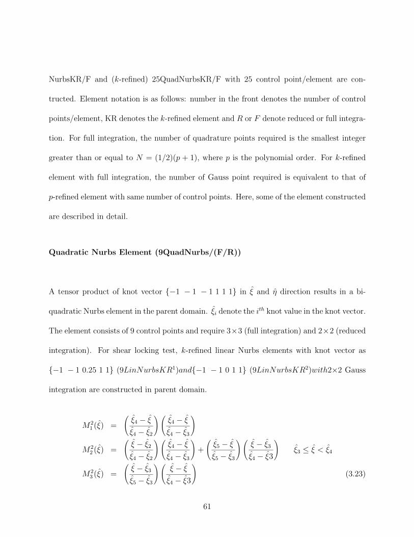
NurbsKR/F and (k-refined) 25QuadNurbsKR/F with 25 control point/element are con-
tructed. Element notation is as follows: number in the front denotes the number of control
points/element, KR denotes the k-refined element and R or F denote reduced or full integra-
tion. For full integration, the number of quadrature points required is the smallest integer
greater than or equal to N = (1/2)(p + 1), where p is the polynomial order. For k-refined
element with full integration, the number of Gauss point required is equivalent to that of
p-refined element with same number of control points. Here, some of the element constructed
are described in detail.
Quadratic Nurbs Element (9QuadNurbs/(F/R))
A tensor product of knot vector −1 − 1 − 1 1 1 1 in ξ and η direction results in a bi-
quadratic Nurbs element in the parent domain. ξi denote the ith knot value in the knot vector.
The element consists of 9 control points and require 3×3 (full integration) and 2×2 (reduced
integration). For shear locking test, k-refined linear Nurbs elements with knot vector as
−1 − 1 0.25 1 1 (9LinNurbsKR1)and−1 − 1 0 1 1 (9LinNurbsKR2)with2×2 Gauss
integration are constructed in parent domain.
M21 (ξ) =
(ξ4 − ξξ4 − ξ2
)(ξ4 − ξξ4 − ξ3
)
M22 (ξ) =
(ξ − ξ2
ξ4 − ξ2
)(ξ4 − ξξ4 − ξ3
)+
(ξ5 − ξξ5 − ξ3
)(ξ − ξ3
ξ4 − ξ3
)ξ3 ≤ ξ < ξ4
M23 (ξ) =
(ξ − ξ3
ξ5 − ξ3
)(ξ − ξξ4 − ξ3
)(3.23)
61

Similarly, the shape functions in η direction are obtained. The product rule yields the
following bi-quadratic shape functions,
R21(ξ, η) = M2
1 (ξ)N21 (η) R2
2(ξ, η) = M21 (ξ)N2
2 (η) R23(ξ, η) = M2
1 (ξ)N23 (η)
R24(ξ, η) = M2
2 (ξ)N21 (η) R2
5(ξ, η) = M22 (ξ)N2
2 (η) R26(ξ, η) = M2
2 (ξ)N23 (η)
R27(ξ, η) = M2
3 (ξ)N21 (η) R2
8(ξ, η) = M23 (ξ)N2
2 (η) R29(ξ, η) = M2
3 (ξ)N23 (η)
(3.24)
Figure 3.3 shows Nurbs basis in ξ and η directions along with the parent element.
Figure 3.3: Quadratic Nurbs element with basis functions in each direction
62
k-refined Quadratic Nurbs element I(16QuadNurbsKR/F)
A tensor product of knot vector −1 − 1 − 1 0 1 1 1 in ξ and η direction results in a bi-
quadratic Nurbs element in the parent domain. The knot vector is divided into two intervals
and shape functions have unique value over each interval. ξi denote the ith knot value in the
knot vector. The shape functions in ξ direction over each interval are derived as follows,
M21 (ξ) =
(ξ4 − ξξ4 − ξ2
)(ξ4 − ξξ4 − ξ3
)
M22 (ξ) =
(ξ − ξ2
ξ4 − ξ2
)(ξ4− ξξ4 − ξ3
)+
(ξ5 − ξξ5 − ξ3
)(ξ − ξ3
ξ4 − ξ3
)ξ3 ≤ ξ < ξ4
M23 (ξ) =
(ξ − ξ3
ξ5 − ξ3
)(ξ − ξξ4 − ξ3
)(3.25)
M24 (ξ) = 0
M21 (ξ) = 0
M22 (ξ) =
(ξ5 − ξξ5 − ξ3
)(ξ5 − ξξ5 − ξ4
)
M23 (ξ) =
(ξ − ξ3
ξ5 − ξ3
)(ξ − ξξ4 − ξ3
)+
(ξ − ξ3
ξ5 − ξ3
)(ξ5 − ξξ5 − ξ3
)ξ4 ≤ ξ < ξ5
M24 (ξ) =
(ξ − ξ4
ξ6 − ξ4
)(ξ4 − ξξ5 − ξ4
)(3.26)
Similarly, the shape functions in the η direction are obtained. The product rule yields the
16 bi-quadratic shape functions, R2k, requiring 4× 4 Gauss points. In k-refinement process,
the order of the existing knot vector is elevated first and then, a knot is inserted instead of
63
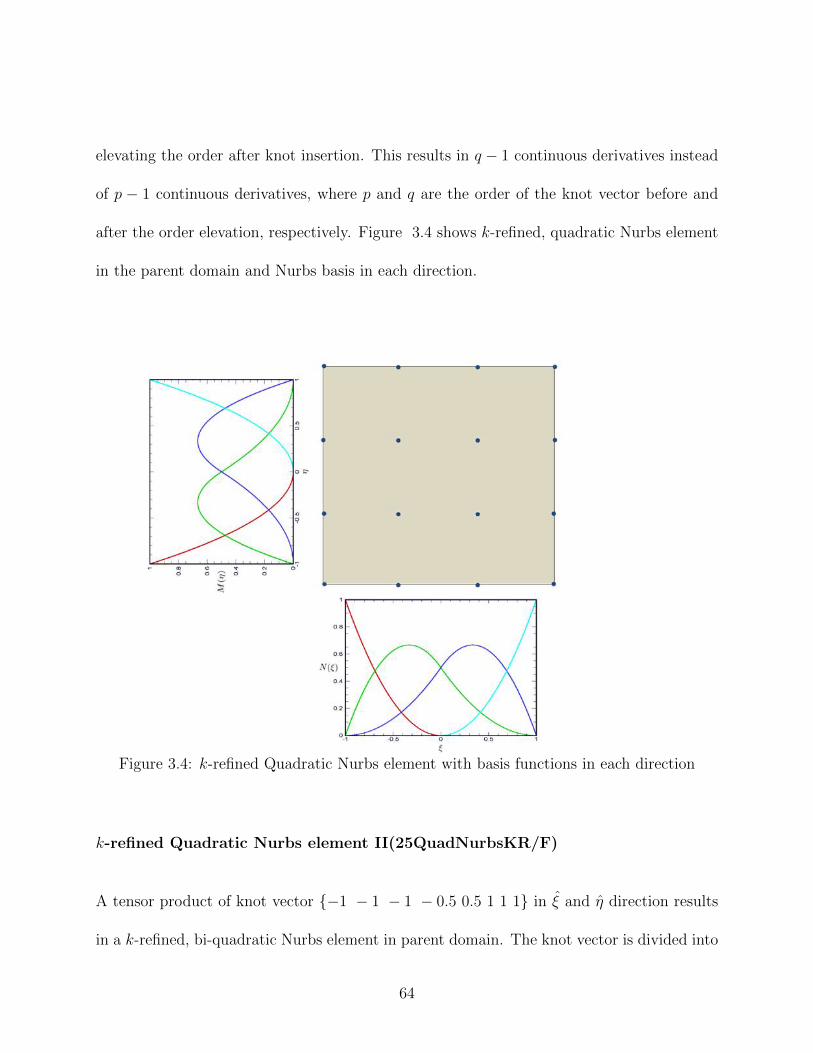
elevating the order after knot insertion. This results in q − 1 continuous derivatives instead
of p − 1 continuous derivatives, where p and q are the order of the knot vector before and
after the order elevation, respectively. Figure 3.4 shows k-refined, quadratic Nurbs element
in the parent domain and Nurbs basis in each direction.
Figure 3.4: k-refined Quadratic Nurbs element with basis functions in each direction
k-refined Quadratic Nurbs element II(25QuadNurbsKR/F)
A tensor product of knot vector −1 − 1 − 1 − 0.5 0.5 1 1 1 in ξ and η direction results
in a k-refined, bi-quadratic Nurbs element in parent domain. The knot vector is divided into
64
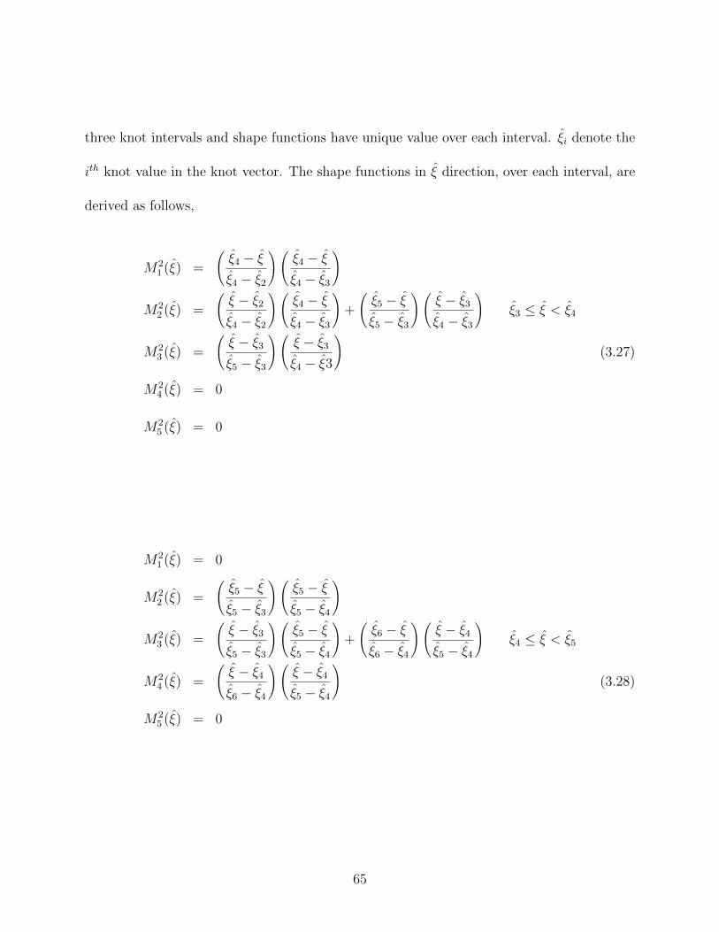
three knot intervals and shape functions have unique value over each interval. ξi denote the
ith knot value in the knot vector. The shape functions in ξ direction, over each interval, are
derived as follows,
M21 (ξ) =
(ξ4 − ξξ4 − ξ2
)(ξ4 − ξξ4 − ξ3
)
M22 (ξ) =
(ξ − ξ2
ξ4 − ξ2
)(ξ4 − ξξ4 − ξ3
)+
(ξ5 − ξξ5 − ξ3
)(ξ − ξ3
ξ4 − ξ3
)ξ3 ≤ ξ < ξ4
M23 (ξ) =
(ξ − ξ3
ξ5 − ξ3
)(ξ − ξ3
ξ4 − ξ3
)(3.27)
M24 (ξ) = 0
M25 (ξ) = 0
M21 (ξ) = 0
M22 (ξ) =
(ξ5 − ξξ5 − ξ3
)(ξ5 − ξξ5 − ξ4
)
M23 (ξ) =
(ξ − ξ3
ξ5 − ξ3
)(ξ5 − ξξ5 − ξ4
)+
(ξ6 − ξξ6 − ξ4
)(ξ − ξ4
ξ5 − ξ4
)ξ4 ≤ ξ < ξ5
M24 (ξ) =
(ξ − ξ4
ξ6 − ξ4
)(ξ − ξ4
ξ5 − ξ4
)(3.28)
M25 (ξ) = 0
65

M21 (ξ) = 0
M22 (ξ) = 0
M23 (ξ) =
(ξ6 − ξξ6 − ξ4
)(ξ6 − ξξ6 − ξ5
)
M24 (ξ) =
(ξ7 − ξξ7 − ξ5
)(ξ − ξ5
ξ6 − ξ5
)ξ5 ≤ ξ < ξ6
M25 (ξ) =
(ξ − ξ5
ξ7 − ξ5
)(ξ − ξ5
ξ6 − ξ5
)(3.29)
The element consists of 25 control functions and require 5×5 Gauss integration points. The
derivatives are q − 1 continuous instead of p − 1 continuous. Figure 3.5 shows the Nurbs
element and the basis in ξ and η directions.
Quartic Nurbs element (25QuarticNurbs/F)
A tensor product of knot vector, −1 − 1 − 1 − 1 − 1 1 1 1 1 1 in ξ and η directions
result in a bi-quartic Nurbs element in the parent domain. Quartic Nurbs element consists
of 25 control points and requires 5× 5 Gauss points. It is equivalent to 25QuadNurbsKR/F
element in terms of number of control points/element and Gauss integration points. The
shape functions in explicit form are not provided here. Figure 3.6 shows the Nurbs element
and basis in ξ and η directions.
66

Figure 3.5: k-refined Quadratic Nurbs element with basis functions in each direction
3.2.5 Geometric nonlinear stiffness matrix
Substituting the displacement field approximation into the weak form, we obtain element
stiffness matrix and load vector. The size of a sub-matrix, K11, in element stiffness matrix,
is (nCP ) × (nCP ) and the size of element load vector, F , is (nCP × dof, 1). nCP stands
for control points per element and dof are the number of degrees of freedom /control point.
Parameters, α and β are the degrees of freedom per control point.
67
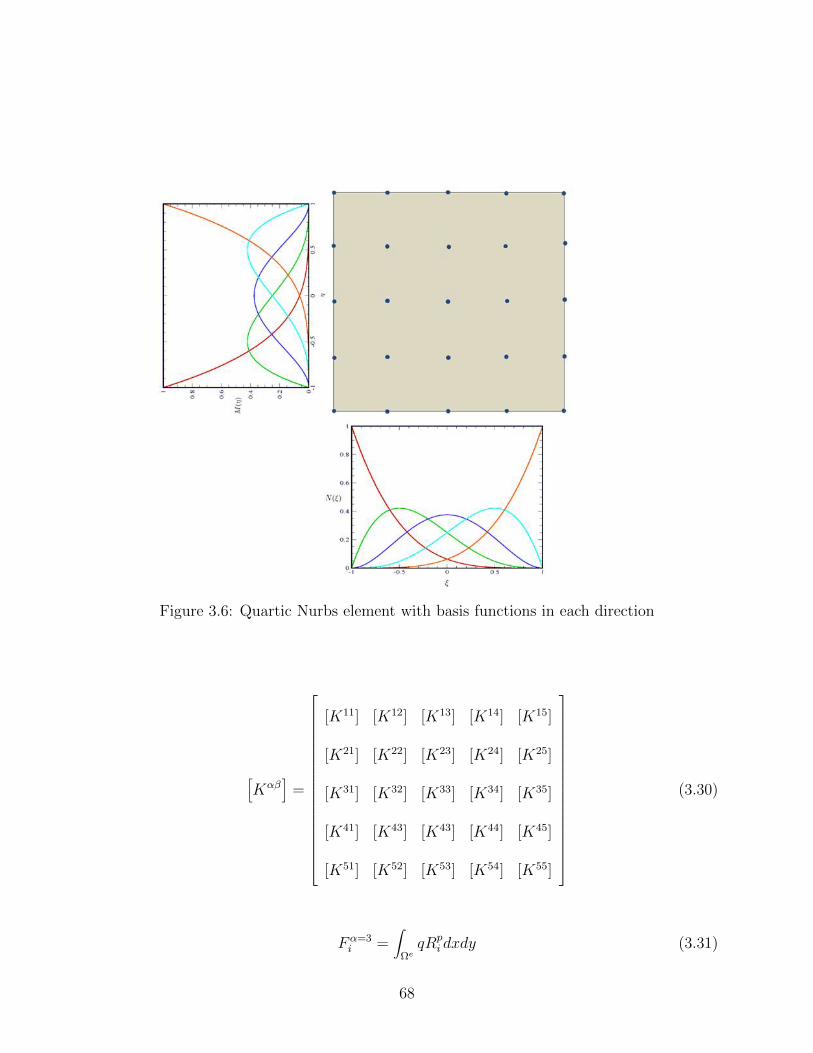
Figure 3.6: Quartic Nurbs element with basis functions in each direction
[Kαβ
]=
[K11] [K12] [K13] [K14] [K15]
[K21] [K22] [K23] [K24] [K25]
[K31] [K32] [K33] [K34] [K35]
[K41] [K43] [K43] [K44] [K45]
[K51] [K52] [K53] [K54] [K55]
(3.30)
Fα=3i =
∫ΩeqRp
i dxdy (3.31)
68

From the element stiffness matrix, the expression for K11, a sub-matrix of element stiffness
matrix, K, is as follows,
K11ij (x, y) =
∫Ωe
[A11
∂Rpi
∂x
∂Rpj
∂x+ A66
∂Rpi
∂y
∂Rpj
∂y+ A16
(∂Rp
i
∂x
∂Rpj
∂y+∂Rp
i
∂y
∂Rpj
∂x
)]dxdy (3.32)
The equation of motion can be written in the matrix form as,
[K] ∆ = F (3.33)
The solution of nonlinear equations is obtained by Newton-Raphson iterative process as
follows,
R (∆) =[KT (∆)
]∆ − F = 0 (3.34)
Tangent stiffness matrix is obtained as,
KT,αβij =
∂Rαi
∂∆βj
KT,αβij =
∂
∂∆βj
5∑γ=1
nCP∑k=1
Kαγik ∆γ
k − Fαi
(3.35)
For example, a sub-matrix in element tangent stiffness matrix is,
KT,33ij =
5∑γ=1
nCP∑k=1
∂K3γik
∂wj∆γk +K33
ij (3.36)
69

The incremental displacement vector is given as,
δ∆ = −[KT (∆r)]−1 Rr (3.37)
And, total displacement vector is obtained as,
∆r+1 = ∆r + δ∆ (3.38)
KT and R are the tangent stiffness and residual load vector. At the beginning of iteration,
r = 0 and nonlinear stiffness terms reduces to zero. The iterative process is continued till
the convergence is obtained within the error tolerance of 10−3. The error norm used for
convergence is as follows, √√√√√√∑NI=1
∣∣∣∆r+1I −∆r
I
∣∣∣2∑NI=1
∣∣∣∆r+1I
∣∣∣2 < 10−3 (3.39)
3.3 Numerical Testing
Isotropic, orthotropic and laminated composite plates are studied here. Geometric nonlin-
earity is accounted for in von-Karman sense, including membrane-bending coupling effects.
Several, thin and moderately thick, isotropic, orthotropic and laminated composite plate
examples are studied for the validation purposes. Different boundary conditions, plate to
thickness ratios and ply angles are considered. Due to bi-axial symmetry, only a quadrant
of the plate is modeled and the center deflections are computed and validated with the liter-
70

ature. The computed center deflection is normalised as w = w/h. Three different boundary
conditions are considered for the analysis.
SS1 : v0 = w0 = φy = 0, at x = a/2;
u0 = w0 = φx = 0, at y = b/2
SS3 : u0 = v0 = w0 = 0 at x = a/2, y = b/2
Clamped : u0 = v0 = w0 = φx = φy = 0; at x = a/2 and y = b/2
symmetry B.C., x = 0, u0 = φx = 0
y = 0, v0 = φy = 0
3.3.1 Clamped Isotropic plate under uniform loading
In this example, a thin a/h = 100, clamped, isotropic square plate under uniform loading
is analyzed. The plate length and thickness are a = 300 in and h = 3 in respectively
and the material properties are E1 = 30E6 psi and ν = 0.316. The center deflection of a
quarter plate is computed and is validated with Levy’s analytical([110]) and Urthaler and
Reddy([39])’s mixed finite element solution. Levy’s solution is considered as a benchmark
solution for validating geometrically nonlinear analysis of thin plates. For most of the ele-
ments tested, solution converged well with the analytical and Reddy’s mixed finite element
solution. Urthaler and Reddy[39] required 4 × 4 mesh of 9 node quadratic element with 7
dof/node to compute the center deflection while 9QuadNurbs/R required 2 × 2 mesh with
5 dof/control point. From the integration point of view, quadratic and cubic Nurbs, with
reduced integration produced equivalent center deflection and higher-order p and k-refined
71

Nurbs element performed equally well using full integration. Similarly, k-refined quadratic
Nurbs elements (25QuadNurbsKR and 16QuadNurbsKR) with full integration produced the
equivalent center deflection as its counterpart 9QuadNurbs/R element did with reduced in-
tegration. Table 3.1 and Fig. 3.7 give the load vs deflection data and the curve, respectively.
Next, the % error in center displacement w.r.t Levy’s solution in nonlinear analysis is plotted
for 9LinNurbsKR2 and quadratic Nurbs elements. % error is greater in the case of 9Quad-
Nurbs/F as compared with 9QuadNurbs/R due to slenderness of the plate. Linear Nurbs
element, 9LinNurbsKR2, seems to perform well due to increased smoothness of basis function
in solution space. Figure 3.8 shows the % error in nonlinear deflection for increasing loads.
Load, p Levy’s Analytical MXFEM/Reddy 9QuadNurbs/R 16QuadNurbsKR 25QuadNurbsKR
0 0 0 0 0 0
17.8 0.237 0.2392 0.2393 0.2354 0.2328
38.3 0.471 0.4738 0.4741 0.4678 0.4635
63.4 0.695 0.6965 0.6975 0.6951 0.6854
95 0.912 0.9087 0.9103 0.9036 0.8985
134.9 1.1210 1.1130 1.1148 1.1092 1.1045
184 1.323 1.308 1.3101 1.3059 1.302
245 1.521 1.501 1.5024 1.4942 1.4969
318 1.714 1.688 1.6885 1.6758 1.6856
402 1.902 1.866 1.8657 1.8662 1.8652
Table 3.1: Comparison of various Nurbs elements, including k-refined with analytical solutionfor clamped, isotropic plate under uniform loading
72

0 100 200 300 400
0
0.5
1
1.5
2
p
w
Levy/Analytical
MixedFE/Reddy
9LinNurbsKR1
9QuadNurbs/R
16QuadNurbsKR/F
Figure 3.7: Load vs deflection curve for a clamped, isotropic plate under increasing uniformload
0 100 200 300 400
0
5
10
15
20
p
%er
ror
(cen
ter
dis
pla
cem
ent)
9QuadNurbs/F
9QuadNurbs/R
16QuadNurbsKR/F
9LinNurbsKR2/F
Figure 3.8: % error in displacement w.r.t Levy’s analytical solution for various Nurbs ele-ments for 2× 2 mesh in nonlinear analysis
73

3.3.2 Shear Locking Test for Thin Plates
Shear locking is the over constraining of element stiffness matrix as the side to thickness
ratio become large, resulting in underestimation of displacement. Shear locking test for
linear analysis is performed with h-refined linear and quadratic Nurbs element for various
a/h ratios and % error in nonlinear displacement w.r.t to Levy’s solution for slender plates
is analyzed.
A square plate with length, L = 10 and material properties as E = 10.92 and ν = 0.3 with
simply-supported boundary condition SS1 under uniform loading for various a/h ratios is
analyzed. % error in center displacement w.r.t reference solution is computed to study the
shear locking effects. Figures 3.9 and 3.10 shows shear locking effect for increasing a/h ratios
for 2× 2 and 3× 3 meshes. Most of the elements perform well for increasing a/h ratios. In
case of k-refined linear Nurbs element, addition of a knot in the knot vector provide increased
smoothness and seems to remove numerical ill-conditioning effects. Quadratic Nurbs element
also performs excellently with full and reduced integration for linear problem.
3.3.3 Simply Supported Isotropic plate under uniform loading
A square plate with length, L = 10 in, thickness, h = 1 in and material properties E1 = 7.8E6
psi and ν = 0.3 with simply-supported boundary conditions, SS1 and SS3, under uniform
74
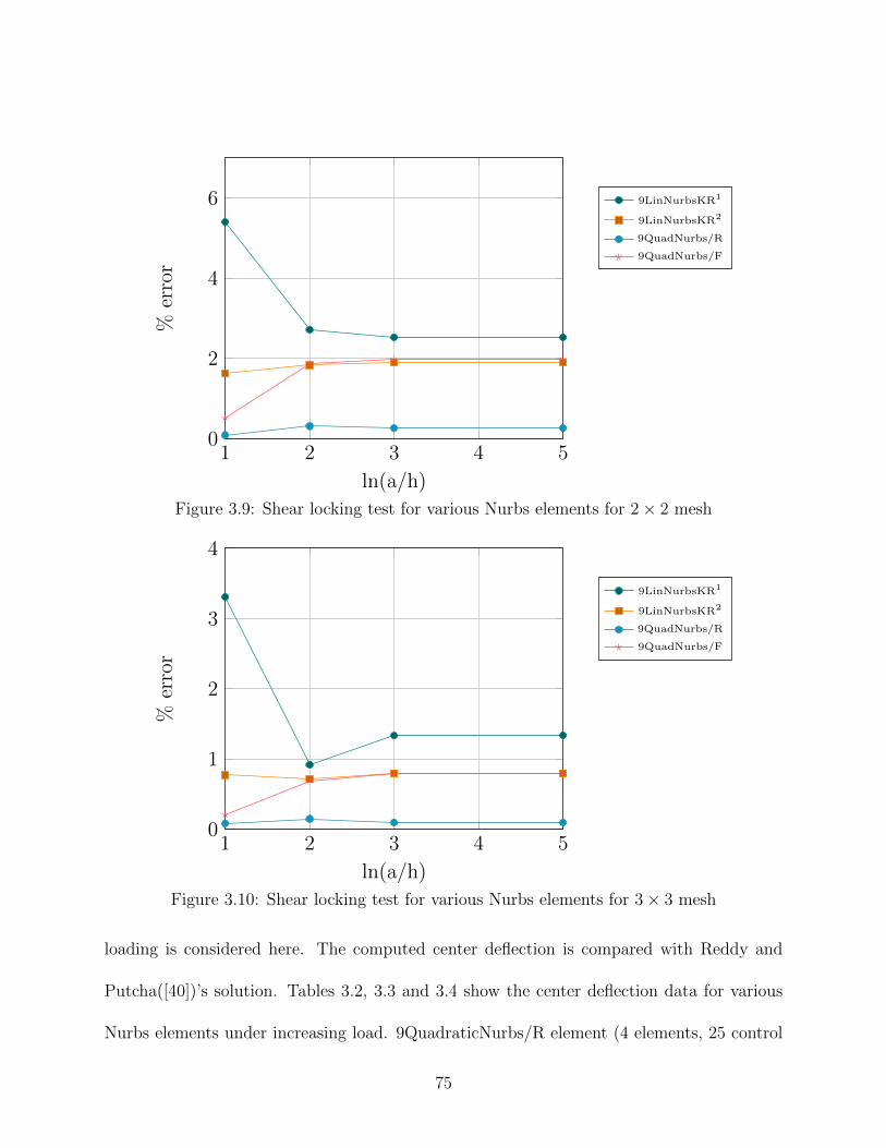
1 2 3 4 50
2
4
6
ln(a/h)
%er
ror
9LinNurbsKR1
9LinNurbsKR2
9QuadNurbs/R
9QuadNurbs/F
Figure 3.9: Shear locking test for various Nurbs elements for 2× 2 mesh
1 2 3 4 50
1
2
3
4
ln(a/h)
%er
ror
9LinNurbsKR1
9LinNurbsKR2
9QuadNurbs/R
9QuadNurbs/F
Figure 3.10: Shear locking test for various Nurbs elements for 3× 3 mesh
loading is considered here. The computed center deflection is compared with Reddy and
Putcha([40])’s solution. Tables 3.2, 3.3 and 3.4 show the center deflection data for various
Nurbs elements under increasing load. 9QuadraticNurbs/R element (4 elements, 25 control
75
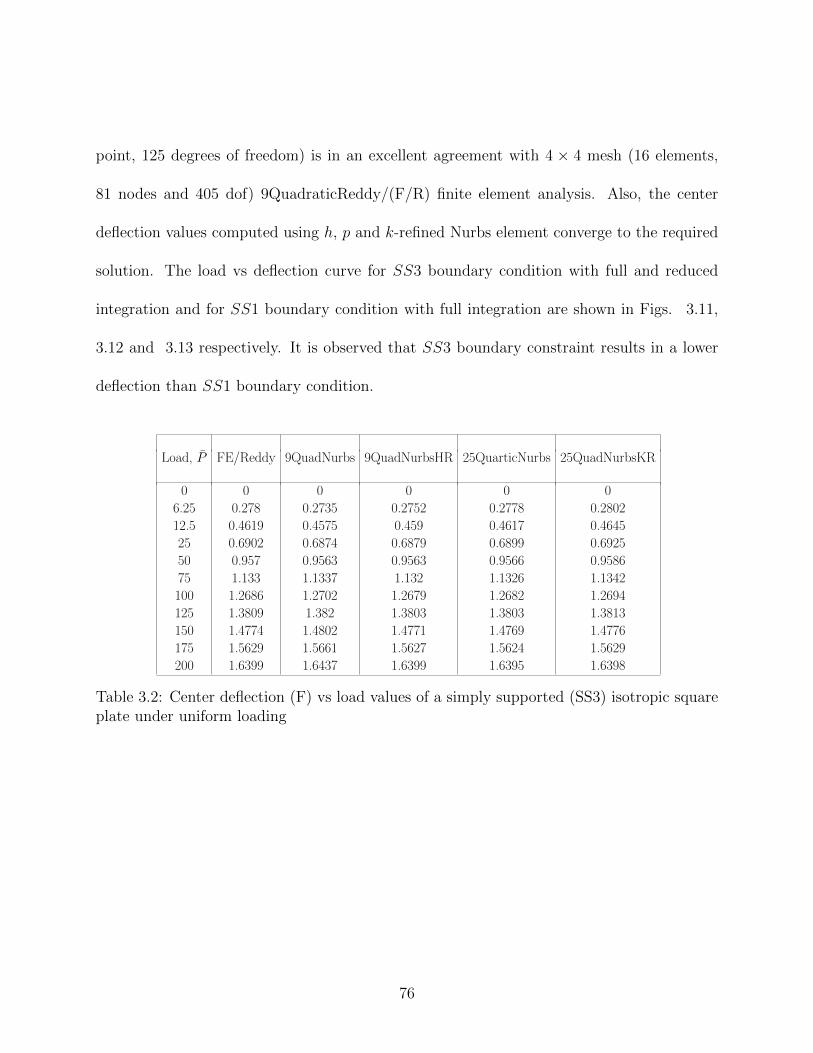
point, 125 degrees of freedom) is in an excellent agreement with 4 × 4 mesh (16 elements,
81 nodes and 405 dof) 9QuadraticReddy/(F/R) finite element analysis. Also, the center
deflection values computed using h, p and k-refined Nurbs element converge to the required
solution. The load vs deflection curve for SS3 boundary condition with full and reduced
integration and for SS1 boundary condition with full integration are shown in Figs. 3.11,
3.12 and 3.13 respectively. It is observed that SS3 boundary constraint results in a lower
deflection than SS1 boundary condition.
Load, P FE/Reddy 9QuadNurbs 9QuadNurbsHR 25QuarticNurbs 25QuadNurbsKR
0 0 0 0 0 0
6.25 0.278 0.2735 0.2752 0.2778 0.2802
12.5 0.4619 0.4575 0.459 0.4617 0.4645
25 0.6902 0.6874 0.6879 0.6899 0.6925
50 0.957 0.9563 0.9563 0.9566 0.9586
75 1.133 1.1337 1.132 1.1326 1.1342
100 1.2686 1.2702 1.2679 1.2682 1.2694
125 1.3809 1.382 1.3803 1.3803 1.3813
150 1.4774 1.4802 1.4771 1.4769 1.4776
175 1.5629 1.5661 1.5627 1.5624 1.5629
200 1.6399 1.6437 1.6399 1.6395 1.6398
Table 3.2: Center deflection (F) vs load values of a simply supported (SS3) isotropic squareplate under uniform loading
76
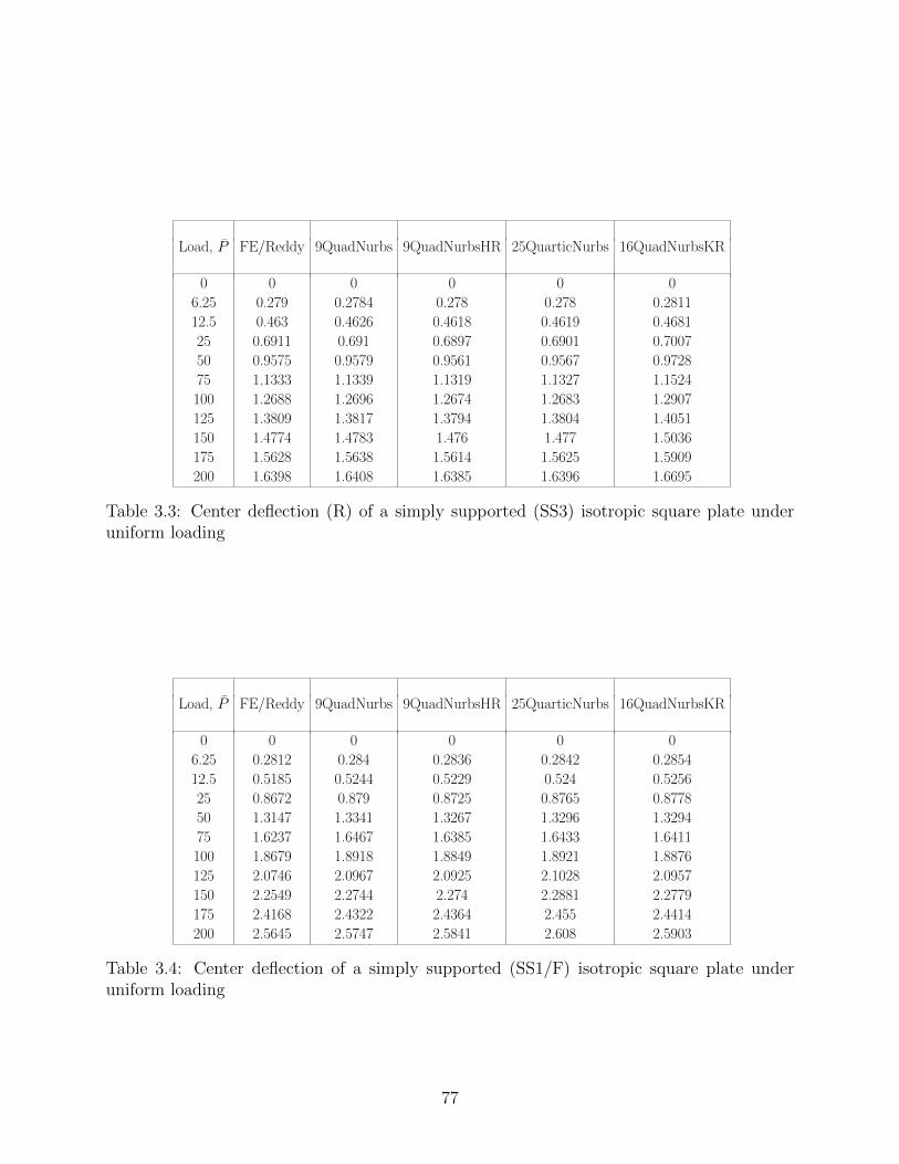
Load, P FE/Reddy 9QuadNurbs 9QuadNurbsHR 25QuarticNurbs 16QuadNurbsKR
0 0 0 0 0 0
6.25 0.279 0.2784 0.278 0.278 0.2811
12.5 0.463 0.4626 0.4618 0.4619 0.4681
25 0.6911 0.691 0.6897 0.6901 0.7007
50 0.9575 0.9579 0.9561 0.9567 0.9728
75 1.1333 1.1339 1.1319 1.1327 1.1524
100 1.2688 1.2696 1.2674 1.2683 1.2907
125 1.3809 1.3817 1.3794 1.3804 1.4051
150 1.4774 1.4783 1.476 1.477 1.5036
175 1.5628 1.5638 1.5614 1.5625 1.5909
200 1.6398 1.6408 1.6385 1.6396 1.6695
Table 3.3: Center deflection (R) of a simply supported (SS3) isotropic square plate underuniform loading
Load, P FE/Reddy 9QuadNurbs 9QuadNurbsHR 25QuarticNurbs 16QuadNurbsKR
0 0 0 0 0 0
6.25 0.2812 0.284 0.2836 0.2842 0.2854
12.5 0.5185 0.5244 0.5229 0.524 0.5256
25 0.8672 0.879 0.8725 0.8765 0.8778
50 1.3147 1.3341 1.3267 1.3296 1.3294
75 1.6237 1.6467 1.6385 1.6433 1.6411
100 1.8679 1.8918 1.8849 1.8921 1.8876
125 2.0746 2.0967 2.0925 2.1028 2.0957
150 2.2549 2.2744 2.274 2.2881 2.2779
175 2.4168 2.4322 2.4364 2.455 2.4414
200 2.5645 2.5747 2.5841 2.608 2.5903
Table 3.4: Center deflection of a simply supported (SS1/F) isotropic square plate underuniform loading
77

0 50 100 150 200
0
0.5
1
1.5
p
w
9QuadFEReddy/F
9QuadNurbs
16CubicNurbs
25QuarticNurbs
25QuadNurbsKR
Figure 3.11: Load vs deflection curve for a simply supported (SS3/F), isotropic plate underincreasing uniform load
0 50 100 150 200
0
0.5
1
1.5
p
w
9QuadFEReddy
9QuadNurbs
16CubicNurbs
25QuarticNurbs
Figure 3.12: Load vs deflection curve for a simply supported (SS3/R), isotropic plate underincreasing uniform load
78

0 50 100 150 200
0
1
2
p
w
9QuadFEReddy
9QuadNurbs
16CubicNurbs
25QuarticNurbs
16QuadNurbsKR
Figure 3.13: Load vs deflection curve for a simply supported (SS1/F), isotropic plate underincreasing uniform load
79

3.3.4 Square, symmetric cross-ply (0/90/90/0) laminated com-
posite plate under uniform loading
A square, symmetric cross-ply (0/90/90/0) laminated composite plate subjected to uniform
loading is considered. The dimensions of the plate are a = 12 in, thickness, t = 0.096 in
and the material properties are E1 = 1.8282e6 psi, E2 = 1.8315e6 psi, G12 = G13 = G23 =
0.3125e6 psi and ν = 0.2395. The center deflection computed using h, p and k-refined Nurbs
elements compare well with those in the literature. The center deflection computed using
Nurbs quadratic element is in excellent agreement with Reddy’s finite element solution ([116])
and requires a lesser number of degrees of freedom. Also, the center deflection is found to be
closer to the experimental curve than Reddy and Putcha([40]) and Zhang([54])’s deflection
response. Table 3.5 and fig. 3.14 shows load vs deflection data and curve.
Load, P FE/Reddy 9QuadNurbs/R 9QuadNurbsHR/R 16CubicNurbs/F 25QuarticNurbs/F
0 0 0 0 0 0
0.2 0.3773 0.3815 0.3781 0.3773 0.3773
0.4 0.6504 0.6573 0.6517 0.6503 0.6504
0.6 0.8489 0.8574 0.8504 0.8486 0.8488
0.8 1.0039 1.0134 1.0054 1.0035 1.00376
1 1.1316 1.142 1.1331 1.131 1.1314
1.2 1.2406 1.2512 1.242 1.24 1.2405
1.4 1.3362 1.3471 1.3378 1.3356 1.3361
1.6 1.4216 1.4328 1.423 1.4211 1.4216
1.8 1.4991 1.5105 1.5007 1.4985 1.4991
2 1.5701 1.58175 1.5717 1.5696 1.5702
2.2 1.6359 1.6477 1.6375 1.6354 1.636
2.4 1.6972 1.7092 1.6988 1.69667 1.6974
Table 3.5: Center deflection(F) of a clamped, square, cross-ply (0/90/90/0), laminated com-posite plate under uniform loading
80
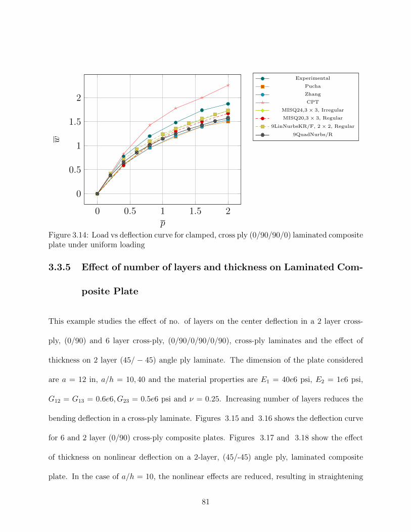
0 0.5 1 1.5 2
0
0.5
1
1.5
2
p
w
Experimental
Pucha
Zhang
CPT
MISQ24,3× 3, Irregular
MISQ20,3× 3, Regular
9LinNurbsKR/F, 2× 2, Regular
9QuadNurbs/R
Figure 3.14: Load vs deflection curve for clamped, cross ply (0/90/90/0) laminated compositeplate under uniform loading
3.3.5 Effect of number of layers and thickness on Laminated Com-
posite Plate
This example studies the effect of no. of layers on the center deflection in a 2 layer cross-
ply, (0/90) and 6 layer cross-ply, (0/90/0/90/0/90), cross-ply laminates and the effect of
thickness on 2 layer (45/ − 45) angle ply laminate. The dimension of the plate considered
are a = 12 in, a/h = 10, 40 and the material properties are E1 = 40e6 psi, E2 = 1e6 psi,
G12 = G13 = 0.6e6, G23 = 0.5e6 psi and ν = 0.25. Increasing number of layers reduces the
bending deflection in a cross-ply laminate. Figures 3.15 and 3.16 shows the deflection curve
for 6 and 2 layer (0/90) cross-ply composite plates. Figures 3.17 and 3.18 show the effect
of thickness on nonlinear deflection on a 2-layer, (45/-45) angle ply, laminated composite
plate. In the case of a/h = 10, the nonlinear effects are reduced, resulting in straightening
81
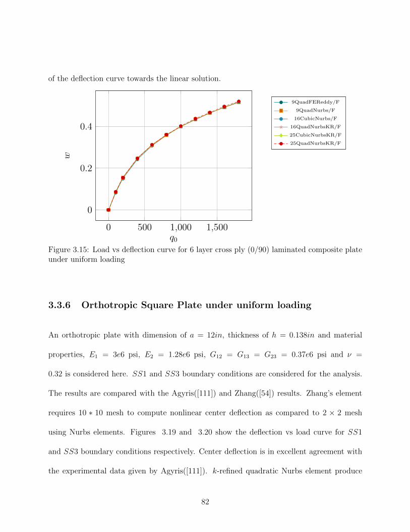
of the deflection curve towards the linear solution.
0 500 1,000 1,500
0
0.2
0.4
q0
w
9QuadFEReddy/F
9QuadNurbs/F
16CubicNurbs/F
16QuadNurbsKR/F
25CubicNurbsKR/F
25QuadNurbsKR/F
Figure 3.15: Load vs deflection curve for 6 layer cross ply (0/90) laminated composite plateunder uniform loading
3.3.6 Orthotropic Square Plate under uniform loading
An orthotropic plate with dimension of a = 12in, thickness of h = 0.138in and material
properties, E1 = 3e6 psi, E2 = 1.28e6 psi, G12 = G13 = G23 = 0.37e6 psi and ν =
0.32 is considered here. SS1 and SS3 boundary conditions are considered for the analysis.
The results are compared with the Agyris([111]) and Zhang([54]) results. Zhang’s element
requires 10 ∗ 10 mesh to compute nonlinear center deflection as compared to 2 × 2 mesh
using Nurbs elements. Figures 3.19 and 3.20 show the deflection vs load curve for SS1
and SS3 boundary conditions respectively. Center deflection is in excellent agreement with
the experimental data given by Agyris([111]). k-refined quadratic Nurbs element produce
82

0 500 1,000 1,500
0
0.2
0.4
0.6
q0
w
9QuadNurbs/F
9QuadNurbsHR/F
16CubicNurbs/F
25QuarticNurbsKR/F
Figure 3.16: Load vs deflection curve for 2 layer cross ply (0/90) laminated composite plateunder uniform loading
0 500 1,000 1,500
0
0.2
0.4
q0
w
9QuadNurbs/R
9QuadNurbsHR/R
16CubicNurbs/R
25QuarticNurbsKR/F
25CubicNurbsKR/F
25QuadNurbsKR/F
Figure 3.17: Load vs deflection curve for angle ply (45/-45) laminated composite plate underuniform loading for a/h = 40
83
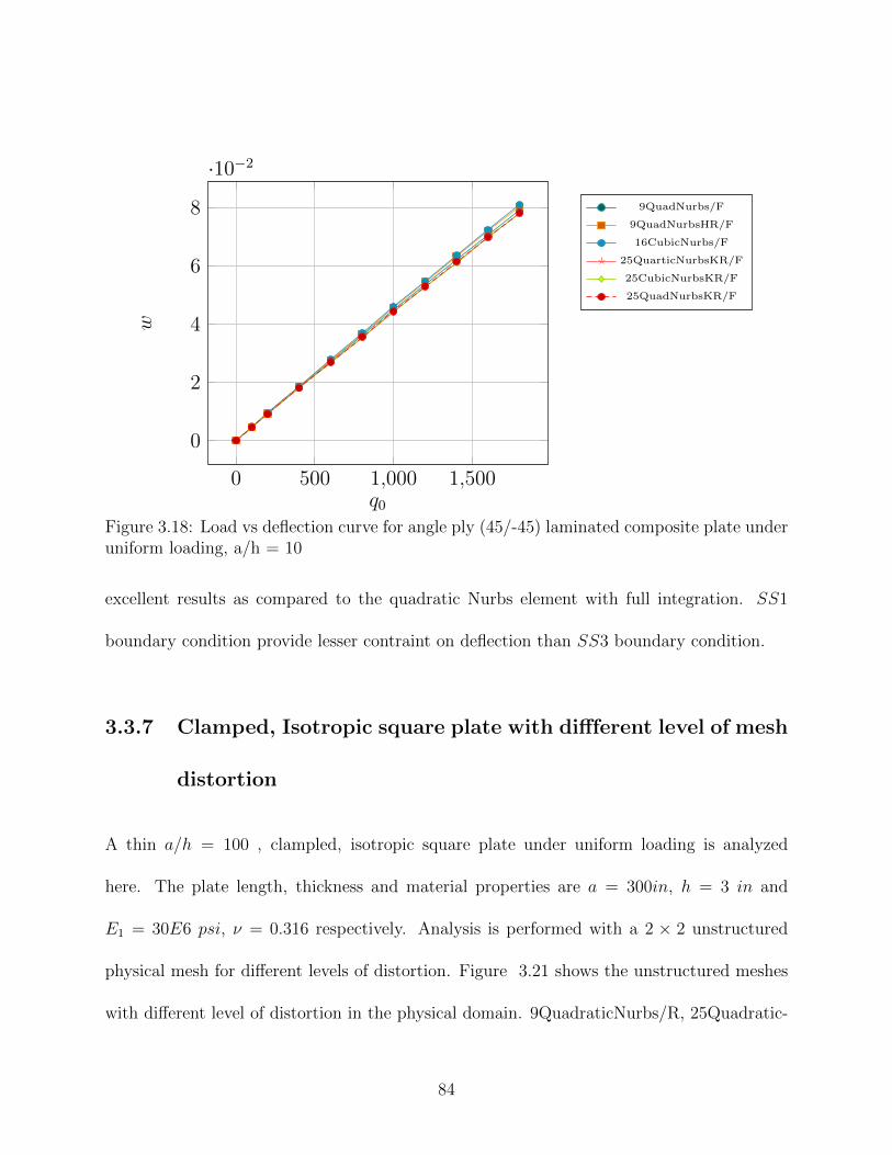
0 500 1,000 1,500
0
2
4
6
8
·10−2
q0
w
9QuadNurbs/F
9QuadNurbsHR/F
16CubicNurbs/F
25QuarticNurbsKR/F
25CubicNurbsKR/F
25QuadNurbsKR/F
Figure 3.18: Load vs deflection curve for angle ply (45/-45) laminated composite plate underuniform loading, a/h = 10
excellent results as compared to the quadratic Nurbs element with full integration. SS1
boundary condition provide lesser contraint on deflection than SS3 boundary condition.
3.3.7 Clamped, Isotropic square plate with diffferent level of mesh
distortion
A thin a/h = 100 , clampled, isotropic square plate under uniform loading is analyzed
here. The plate length, thickness and material properties are a = 300in, h = 3 in and
E1 = 30E6 psi, ν = 0.316 respectively. Analysis is performed with a 2 × 2 unstructured
physical mesh for different levels of distortion. Figure 3.21 shows the unstructured meshes
with different level of distortion in the physical domain. 9QuadraticNurbs/R, 25Quadratic-
84
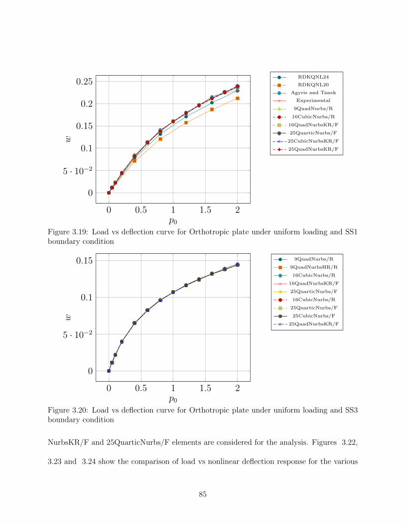
0 0.5 1 1.5 2
0
5 · 10−2
0.1
0.15
0.2
0.25
p0
wRDKQNL24
RDKQNL20
Agyris and Tanek
Experimental
9QuadNurbs/R
16CubicNurbs/R
16QuadNurbsKR/F
25QuarticNurbs/F
25CubicNurbsKR/F
25QuadNurbsKR/F
Figure 3.19: Load vs deflection curve for Orthotropic plate under uniform loading and SS1boundary condition
0 0.5 1 1.5 2
0
5 · 10−2
0.1
0.15
p0
w
9QuadNurbs/R
9QuadNurbsHR/R
16CubicNurbs/R
16QuadNurbsKR/F
25QuarticNurbs/F
16CubicNurbs/R
25QuarticNurbs/F
25CubicNurbs/F
25QuadNurbsKR/F
Figure 3.20: Load vs deflection curve for Orthotropic plate under uniform loading and SS3boundary condition
NurbsKR/F and 25QuarticNurbs/F elements are considered for the analysis. Figures 3.22,
3.23 and 3.24 show the comparison of load vs nonlinear deflection response for the various
85

Nurbs elements. 9QuadraticNurbs/R element exhibit hourglass instability as the deflection
response increases with each level of mesh distortion due to under-integrated stiffness matrix.
However, k-refined quadratic and higher order Nurbs element with full integration produce
a stabilized nonlinear deflection vs load response i.e. element does not exhibit hourglass
instability without increasing the order of the polynomial.
Figure 3.21: Physical meshes with different level of mesh distortion for a clamped, Isotropic,square plate
3.4 Conclusions
Geometrically nonlinear Nurbs Isogeometric finite element analysis of laminated composite
plate is presented here. h, p and k-refinement techniques are utilized and various lower and
86

0 100 200 300 400
0
0.5
1
1.5
2
p
w
Levy’s Analytical Solution
9QuadNurbs/R, Structured
9QuadNurbs/R, Unstructured1
9QuadNurbs/R, Unstructured2
9QuadNurbs/R, Unstructured3
Figure 3.22: Mesh distortion sensitivity test using 9QuadNurbs/R element for 2× 2 mesh
0 100 200 300 400
0
0.5
1
1.5
2
p
w
Levy’s Analytical Solution
25QuadNurbsKR/F, Structured
25QuadNurbsKR/F, Unstructured1
25QuadNurbsKR/F, Unstructured2
25QuadNurbsKR/F, Unstructured3
Figure 3.23: Mesh distortion sensitivity test using 25QuadNurbsKR/F element for 2 × 2mesh
87

0 100 200 300 400
0
0.5
1
1.5
2
p
w
Levy’s Analytical
25QuarticNurbs/F, Structured
25QuarticNurbs/F, Unstructured1
25QuarticNurbs/F, Unstructured2
25QuarticNurbs/F, Unstructured3
Figure 3.24: Mesh distortion sensitivity test using 25QuarticNurbs/F element for 2×2 mesh
0 100 200 300 400
0
2
4
6
p
%er
ror
(cen
ter
dis
pla
cem
ent)
9QuadNurbs/R, Unstructured1
25QuadNurbsKR/F, Unstructured1
25QuarticNurbs/F, Unstructured1
9QuadNurbs/R, Unstructured2
25QuadNurbsKR/F, Unstructured2
25QuarticNurbs/F, Unstructured2
9QuadNurbs/R, Unstructured3
25QuadNurbsKR/F, Unstructured3
25QuarticNurbs/F, Unstructured3
Figure 3.25: % error (center displacement) w.r.t structured mesh in Mesh distortion sensi-tivity test
88

higher-order elements are contructed. Numerical results are presented for thin to moderately
thick plates for various length to thickness ratios, ply-angles and boundary conditions. The
computed center deflection is found to be in excellent agreement with the literature and
requires fewer degrees of freedom/control points when compared with regular finite element
analysis. For thin plates analysis, k-refined, quadratic Nurbs element remedies the shear
locking problem and removes hourglass instability experienced in reduced integrated Nurbs
and regular finite element analysis, though at the expense of computational time.
89
Chapter 4
Interlaminar Stress Recovery by
Direct Post-Processing in Nurbs
Isogeometric Finite Element
Framework
This chapter describes the development of Nurbs post-processor for in-plane and interlaminar
stress calculation in laminated composite and sandwich plates. First-order, shear-deformable
laminate composite plate theory is utilized in deriving the governing equations using a vari-
ational formulation. Linear, quadratic, higher order and k-refined Nurbs elements are con-
structed and numerical validation is performed for orthotropic, laminated composite and
90

sandwich plates. Lagrange finite element suffers from higher order stress gradient oscillations
due to Gibbs phenomenon and require alternative stress recovery procedures for accurate
interlaminar stress calculations, especially interlaminar normal stress. In this chapter, direct
Nurbs based post-processing is performed which computes the interlaminar shear and normal
stresses from higher order gradients of Nurbs basis in a single step procedure. The stresses
are found to be in an excellent agreement with 3D elasticity solution. FSDT along with k-
refinement procedure of Nurbs basis computes equivalent or better stresses than higher-order
shear deformation theory.
4.1 First-order shear deformation plate theory for Lam-
inated Composite Plates
4.1.1 Governing Equations
The origin of material coordinate system is considered to be the mid-plane of the laminate
and Kirchhoff assumption that the transverse normal remain perpendicular to the mid-
surface after deformation is relaxed. However, transverse strain, εz, and out-of plane normal
stress, σz are considered negeligible. Layers are assumed to be perfectly bonded. Figure 6.1
shows the coordinate system and layer numbering of a laminated composite plate. Figure 6.2
shows the undeformed and deformed configuration of first order shear-deformable laminated
composite plate. The displacement field is defined as,
91

u(x, y, z) = u0(x, y) + zφx(x, y)
v(x, y, z) = v0(x, y) + zφy(x, y) (4.1)
w(x, y, z) = w0(x, y)
where u0, v0, w0, are the displacement along the x, y and z-axis and φx, φy are the rotation
of transverse normal of the mid-plane about the y and x-axis respectively.
x
yz
kh/2
h/2
Figure 4.1: Coordinate system and layer numbering used for a laminate plate
Total in-plane strain ε is decomposed into membrane and bending strains.
ε = εm + zεb (4.2)
92

Figure 4.2: Undeformed and deformed configuration of first order shear-deformable plate
εm, the membrane strain can be written as follows,
εm =
εmx
εmy
γmxy
=
∂u0∂x
∂v0∂y
∂u0∂y
+ ∂v0∂x
(4.3)
εb, the bending strain can be written as follows,
εb =
εbx
εby
γbxy
=
∂φy∂y
∂φy∂y
∂φx∂y
+ ∂φy∂x
(4.4)
93
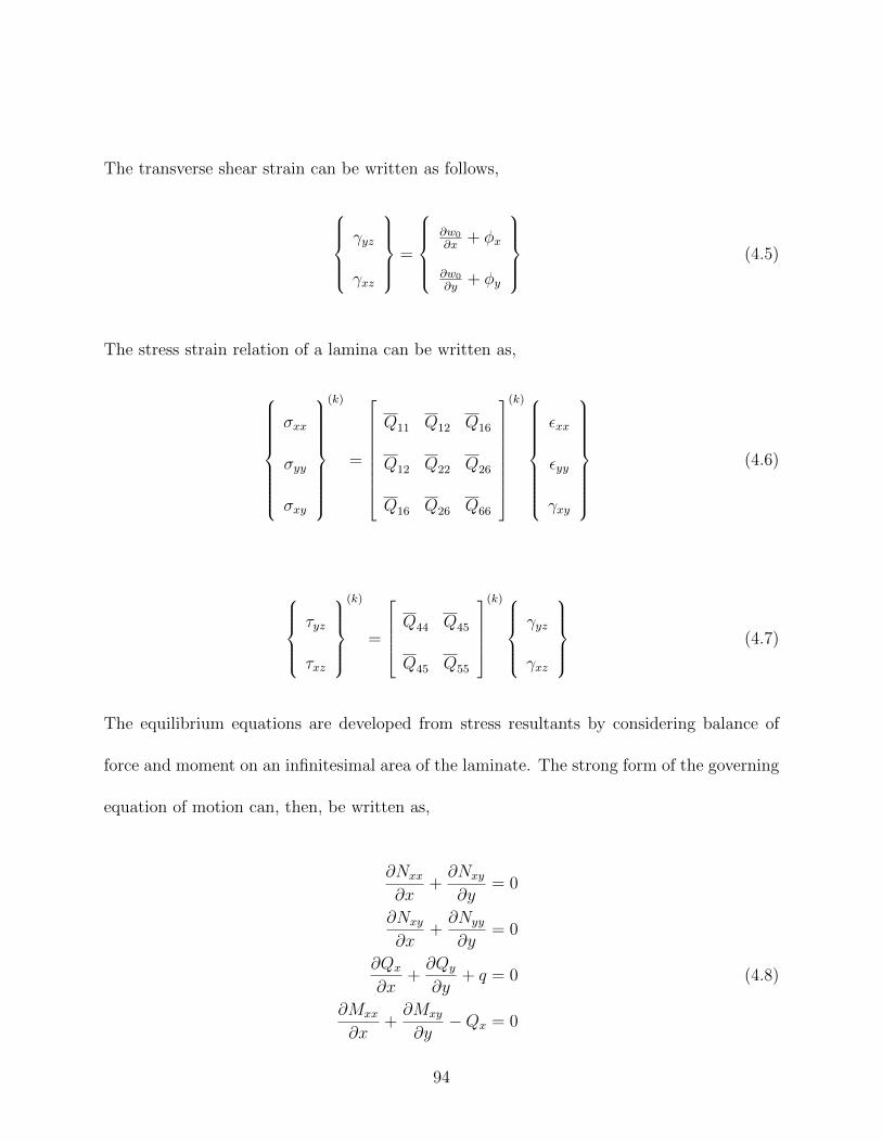
The transverse shear strain can be written as follows,
γyz
γxz
=
∂w0
∂x+ φx
∂w0
∂y+ φy
(4.5)
The stress strain relation of a lamina can be written as,
σxx
σyy
σxy
(k)
=
Q11 Q12 Q16
Q12 Q22 Q26
Q16 Q26 Q66
(k)
εxx
εyy
γxy
(4.6)
τyz
τxz
(k)
=
Q44 Q45
Q45 Q55
(k)
γyz
γxz
(4.7)
The equilibrium equations are developed from stress resultants by considering balance of
force and moment on an infinitesimal area of the laminate. The strong form of the governing
equation of motion can, then, be written as,
∂Nxx
∂x+∂Nxy
∂y= 0
∂Nxy
∂x+∂Nyy
∂y= 0
∂Qx
∂x+∂Qy
∂y+ q = 0 (4.8)
∂Mxx
∂x+∂Mxy
∂y−Qx = 0
94
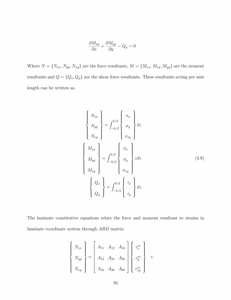
∂Mxy
∂x+∂Myy
∂y−Qy = 0
Where N = Nxx, Nyy, Nxy are the force resultants, M = Mxx,Mxy,Myy are the moment
resultants and Q = Qx, Qy are the shear force resultants. These resultants acting per unit
length can be written as,
Nxx
Nyy
Nxy
=∫ h/2
−h/2
σx
σy
σxy
dz
Mxx
Myy
Mxy
=∫ h/2
−h/2
σx
σy
σxy
zdz (4.9)
Qx
Qy
=∫ h/2
−h/2
τx
τy
dz
The laminate constitutive equations relate the force and moment resultant to strains in
laminate coordinate system through ABD matrix.
Nxx
Nyy
Nxy
=
A11 A12 A16
A12 A22 A26
A16 A26 A66
εmx
εmy
εmxy
+
95

B11 B12 B16
B12 B22 B26
B16 B26 B66
εbx
εby
εbxy
(4.10)
Mxx
Myy
Mxy
=
B11 B12 B16
B12 B22 B26
B16 B26 B66
εmx
εmy
εmxy
+
D11 D12 D16
D12 D22 D26
D16 D26 D66
εbx
εby
εbxy
(4.11)
Qy
Qx
= kk
A44 A45
A45 A55
γyz
γxz
(4.12)
(Aij, Bij, Dij) =N∑k=1
(Qkij (zk+1 − zk) ,
1
2Qkij
(z2k+1 − z2
k
),1
3Qkij
(z3k+1 − z3
k
))
(A44, A45, A55) =N∑k=1
(Qk
44, Qk
45, Qk
55
)(zk+1 − zk) (4.13)
96

In ABD matrix, Aij, Bij and Dij terms represent extensional and shear, extensional-bending
coupling and bending stiffness terms and Qkijs are plane-stress reduced stiffness terms. kk is
the shear correction factor.
Weak form of the governing equations is obtained by pre-multipying the equation of motion
with δu0, δv0, δw0, δφx and δφy respectively and integrating by parts over the element
domain. Substituting force, moment and shear force resultant,
0 =∫
Ωe
(∂δu0
∂xNxx +
∂δu0
∂yNyy
)dxdy −
∮ΓePxδu0ds
0 =∫
Ωe
(∂δv0
∂xNxy +
∂δv0
∂yNyy
)dxdy −
∮ΓePyδu0ds
0 =∫
Ωe
[∂δw0
∂xQx +
∂δW0
∂yQy − δw0q +
∂δw0
∂x
(Nxx
∂δw0
∂x+ Nxy
∂δw0
∂y
)
+∂δw0
∂y
(Nxy
∂δw0
∂x+ Nyy
∂δw0
∂y
)]dxdy
0 −∮
Γe
[(Qx + Nxx
∂δw0
∂x+ Nxy
∂δw0
∂y
)nx +
(Qy + Nxy
∂δw0
∂x+ Nyy
∂δw0
∂y
)ny
]δw0ds
0 =∫
Ωe
(∂δφx∂x
Mxx +∂δφx∂y
Mxy + δφxQx
)dxdy −
∮ΓeTxδφxds (4.14)
0 =∫
Ωe
(∂δφy∂x
Mxy +∂δφy∂y
Myy + δφyQy
)dxdy −
∮ΓeTyδφyds0
And, the secondary variables are given as,
Px = Nxxnx +Nxyny, Py = Nxynx +Nyyny
Tx = Mxxnx +Mxyny, Ty = Mxynx +Myyny (4.15)
Qn =
(Qx + Nxx
∂w0
∂x+ Nxy
∂w0
∂y
)nx +
(Qy + Nxy
∂w0
∂x+ Nyy
∂w0
∂y
)ny
97
where nx and ny are the directional cosines of the outward normal vector.
4.2 Linear Nurbs Isogeometric Finite Element Formu-
lation
4.2.1 Finite Element Model
The dependent displacement field variables are approximated by Nurbs basis functions as
follows,
u0(x, y) =nCP∑j=1
ujRj(x(ξ, η), y(ξ, η)); v0(x, y) =nCP∑j=1
vjRj(x(ξ, η), y(ξ, η))
w0(x, y) =nCP∑j=1
wjRj(x(ξ, η), y(ξ, η)) (4.16)
φx(x, y) =nCP∑j=1
φxjRj(x(ξ, η), y(ξ, η));φy(x, y) =nCP∑j=1
φyjRj(x(ξ, η), y(ξ, η))
where nCP are the number of control points per element and Rj are 2D Nurbs basis.
Substituting the displacement field approximation into the weak form, we obtain element
stiffness matrix and load vector. For instance, the size of a sub-matrix, K11, in element
stiffness matrix, is (nCP )× (nCP ) and the size of element load vector, F , is (nCP ×dof, 1).
nCP stands for control points per element, dof are the no. of degrees of freedom /control
point and (α, β = 1, 2, ....5).
98

[Kαβ
]=
[K11] [K12] [K13] [K14] [K15]
[K21] [K22] [K23] [K24] [K25]
[K31] [K32] [K33] [K34] [K35]
[K41] [K43] [K43] [K44] [K45]
[K51] [K52] [K53] [K54] [K55]
(4.17)
Fα=3i =
∫ΩeqRp
i dxdy (4.18)
From the element stiffness matrix, the expression for K11, a sub-matrix of element stiffness
matrix, K, is as follows,
K11ij =
∫Ωe
[A11
∂Rpi
∂x
∂Rpj
∂x+ A66
∂Rpi
∂y
∂Rpj
∂y+ A16
(∂Rp
i
∂x
∂Rpj
∂y+∂Rp
i
∂y
∂Rpj
∂x
)]dxdy (4.19)
The equation of motion can be written in the matrix form as,
[K] ∆ = F (4.20)
4.2.2 Nurbs Basis
This subsection details bspline and rational basis generation and describes the transformation
from physical to parametric to parent domain. The p and k-refined Nurbs elements are
99

constructed by modifying the knot vector by knot-insertion. Last part of this subsection
describes the construction of various elements.
B-spline Basis
A knot vector in one dimension is a set of co-ordinates in the parametric space,
Ξ = ξ1, ξ2, ......, ξn+p+1, where ξi is the ith knot, i is the knot index where i = 1, 2, ....., n+
p + 1, p is the order of the polynomial and n is the number of basis functions. The order
of the polynomial, p = 0, 1, 2, 3...., refer to the constant, linear, quadratic, cubic piecewise
polynomials, respectively. If more than one knot is located at the same parametric co-
ordinate, these are termed as repeated knots. In case of the open knot vector, first and
last knots are repeated p + 1 times. Basis function formed using the open knot vector are
interpolatory at the beginning and end of the parametric space interval, i.e. [ξ1, ξn+p+1].
This distinguishes the knots from the nodes in the finite element analysis as all the nodes
are interpolatory. As a starting point, bspline basis functions are defined recursively using
Cox-Deboor algorithm, starting with piecewise constants (p = 0).
Npi (ξ) =
1 if ξi ≤ ξ < ξi+1,
0 otherwise
(4.21)
And, subsequently, basis functions for orders p = 1, 2, 3, ....., are defined as follows,
Npi (ξ) =
ξ − ξiξi+p − ξi
Np−1i (ξ) +
ξi+p+1 − ξξi+p+1 − ξi+1
Np−1i+1 (ξ) (4.22)
100

Rational B-spline (Nurbs) Basis
2D Nurbs basis are formed by tensor product of B-spline basis in ξ and η direction and
using projective weights associated with the control points. Rational basis are very similar
to B-spline basis and derive the continuity and support for the function from the knot vector.
Also, Nurbs basis form a partition of unity and are pointwise non-negative. These properties
result in a strong convex hull property. Rational basis are formed as follows,
Rp,qi,j (ξ, η) =
Npi (ξ)M q
j (η)Wi,j∑CPwi=1
∑CPui=1 Np
i (ξ)M qj (η)Wi,j
(4.23)
Nurbs surface is defined as,
S(x, y) =CPw∑j=1
CPu∑i=1
Rp,qi,j (ξ, η)Bi,j (4.24)
where Npi (ξ) and M q
j (η) are the B-spline basis in ξ and η directions respectively and Rp,qi,j
denote 2D Nurbs basis function. CPw and CPu are the number of control points in ξ and
η directions respectively and nCP = CPu× CPw is the total number of control points per
element. Wi,js are the weights associated with the control points, Bi,j and weights are the
vertical coordinates of the corresponding control points.
101

4.2.3 Numerical Integration
A multi-element patch, a tensor product of knot vectors in ξ and η directions, i.e. 0 0 0.5 1 1×
0 0 0.5 1 1, creates a 2× 2 plate mesh in physical domain. Nurbs basis multiplied with
respective control points constructs a geometric model of plate. In order to perform nu-
merical integration, Guass quadrature is employed. The integration on physical domain is
performed by transformation from physical to parametric and from parametric to parent
domain. Mapping between physical and parametric domain is performed as follows,
x
y
=nCP∑k=1
R1k(ξ, η)
Bxk
Byk
∂Rpk
∂x
∂Rpk
∂y
= [J−1]
∂Rp
k(ξ,η)∂ξ
∂Rpk(ξ,η)∂η
[J ] =
∂x∂ξ
∂y∂ξ
∂x∂η
∂y∂η
(4.25)
Bxk and Byk are control point coordinates and Jxξyη is the mapping from physical to para-
metric domain. The Mapping from parametric to parent domain is the standard mapping
as is done in finite element. Figure 6.3 shows schematic of Isogeometric framework.
102

Figure 4.3: Mapping between physical and parent domain: a framework for Isogeometricfinite element analysis
4.2.4 Nurbs Elements
Various lower and higher order Nurbs elements are constructed by utilizing various refinement
techniques. Linear Nurbs element, 9LinNurbs/F, with 9 control point (i.e. with a knot
insertion at locations such as 0 , 0.25 or 0.5 in knot vector), quadratic Nurbs
element, 9QuadNurbs/(F/R), with 9 control points and k-refined, quadratic Nurbs element,
16QuadNurbsKR/F, with 16 control point are developed. Element notation is as follows:
number in the front denotes the number of control points/element, KR denotes the k-refined
103

element. A few Nurbs elements construction is detailed here.
Quadratic Nurbs Element (9QuadNurbs))
A tensor product of knot vector −1 − 1 − 1 1 1 1 in ξ and η direction results in a bi-
quadratic Nurbs element in the parent domain. ξi denote the ith knot value in the knot
vector. The element consists of 9 control points. The shape function in ξ direction can be
written as follows,
M21 (ξ) =
(ξ4 − ξξ4 − ξ2
)(ξ4 − ξξ4 − ξ3
)
M22 (ξ) =
(ξ − ξ2
ξ4 − ξ2
)(ξ4 − ξξ4 − ξ3
)+
(ξ5 − ξξ5 − ξ3
)(ξ − ξ3
ξ4 − ξ3
)ξ3 ≤ ξ < ξ4
M23 (ξ) =
(ξ − ξ3
ξ5 − ξ3
)(ξ − ξξ4 − ξ3
)(4.26)
Similarly, the shape functions in η direction are obtained. The product rule yields the
following bi-quadratic shape functions,
R21(ξ, η) = M2
1 (ξ)N21 (η) R2
2(ξ, η) = M21 (ξ)N2
2 (η) R23(ξ, η) = M2
1 (ξ)N23 (η)
R24(ξ, η) = M2
2 (ξ)N21 (η) R2
5(ξ, η) = M22 (ξ)N2
2 (η) R26(ξ, η) = M2
2 (ξ)N23 (η)
R27(ξ, η) = M2
3 (ξ)N21 (η) R2
8(ξ, η) = M23 (ξ)N2
2 (η) R29(ξ, η) = M2
3 (ξ)N23 (η)
(4.27)
104
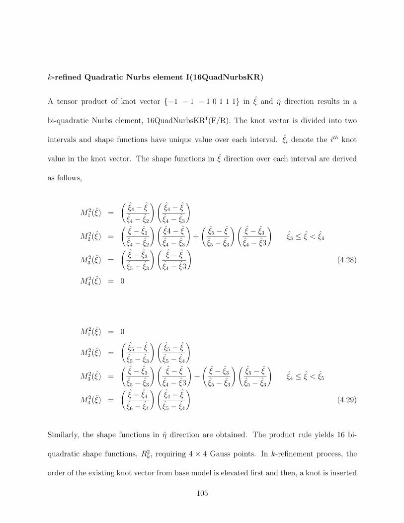
k-refined Quadratic Nurbs element I(16QuadNurbsKR)
A tensor product of knot vector −1 − 1 − 1 0 1 1 1 in ξ and η direction results in a
bi-quadratic Nurbs element, 16QuadNurbsKR1(F/R). The knot vector is divided into two
intervals and shape functions have unique value over each interval. ξi denote the ith knot
value in the knot vector. The shape functions in ξ direction over each interval are derived
as follows,
M21 (ξ) =
(ξ4 − ξξ4 − ξ2
)(ξ4 − ξξ4 − ξ3
)
M22 (ξ) =
(ξ − ξ2
ξ4 − ξ2
)(ξ4− ξξ4 − ξ3
)+
(ξ5 − ξξ5 − ξ3
)(ξ − ξ3
ξ4 − ξ3
)ξ3 ≤ ξ < ξ4
M23 (ξ) =
(ξ − ξ3
ξ5 − ξ3
)(ξ − ξξ4 − ξ3
)(4.28)
M24 (ξ) = 0
M21 (ξ) = 0
M22 (ξ) =
(ξ5 − ξξ5 − ξ3
)(ξ5 − ξξ5 − ξ4
)
M23 (ξ) =
(ξ − ξ3
ξ5 − ξ3
)(ξ − ξξ4 − ξ3
)+
(ξ − ξ3
ξ5 − ξ3
)(ξ5 − ξξ5 − ξ3
)ξ4 ≤ ξ < ξ5
M24 (ξ) =
(ξ − ξ4
ξ6 − ξ4
)(ξ4 − ξξ5 − ξ4
)(4.29)
Similarly, the shape functions in η direction are obtained. The product rule yields 16 bi-
quadratic shape functions, R2k, requiring 4 × 4 Gauss points. In k-refinement process, the
order of the existing knot vector from base model is elevated first and then, a knot is inserted
105

instead of elevating the order after knot insertion. This results in q−1 continuous derivatives
instead of p−1 continuous derivatives, where p and q are the order of the knot vector before
and after order elevation respectively.
For interlaminar stress calculation, two other modifications of k-refined quadratic Nurbs
elements, 16quadNURBKR, are formulated by a single knot insertion in the knot vector at
different locations. 16QuadNurbsKR2 and 16QuudNUUBSKR3 Nurbs elements are formed
by a tensor product of knot vectors, −1 − 1 − 1 0.25 1 1 1 and 1 1 1 0.5 1 1 1 in ξ and
η directions, respectively.
4.3 Calculation of Interlaminar Stresses
The evaluation of transverse stresses τxz and σzz from the stress-strain constitutive relations
leads to discontinuity at the interface of the two adjacent layers of the laminate. Three-
dimensional analysis is very complex due to variation in constitutive laws in the thickness
direction and continuity requirement of transverse stresses and displacement across the in-
terface. Therefore, 3D elasticity equilibrium equations are used to calculate the transverse
stresses in the kth lamina and the equations are given as,
∂σkxx∂x
+∂σkxy∂y
+∂τ kxz∂z
= 0
∂σkxyx∂x
+∂σkyy∂y
+∂τ kyz∂z
= 0 (4.30)
∂τ kxz∂x
+∂τ kyz∂y
+∂σkzz∂z
= 0
106

The stresses are calculated using the direct integration method. It can be seen that the
equations for transverse shear stress, τxz and τyz are a first-order equation. Since, in general,
the transverse shear stresses are known at the top and bottom of the laminate, one can only
obtain a non-unique solution as both the traction boundary conditions can not be enforced
simultaneously. However, for the transverse normal stresses, a second-order equation is
derived and requires double integration through the thickness.
The transverse stress can be computed directly as follows,
τxz = −∫ z
zk
(∂σxx∂x
+∂σxy∂y
)dz + C1
τyz = −∫ z
zk
(∂σxy∂x
+∂σyy∂y
)dz + C2 (4.31)
σzz =∫ z
zk
(∫z
(∂2σxx∂x2
+∂2σyy∂y2
+ 2∂2τxy∂x∂y
)dz
)dz + zC3 + C4
where C1, C2, C3 and C4 are the constants of integration and are obtained by satisfaction of
traction boundary and interface continuity conditions.
4.4 Numerical Testing
Laminated composite and sandwich plates are studied for validation purposes. Different
boundary conditions, plate to thickness ratios and anti-symmetric angle ply composite lam-
107
inated plate are considered. Due to bi-axial symmetry, only a quadrant of the plate is
modeled and deflection and interlaminar stresses are computed at nearest Gauss points of
specific location.
4.4.1 Simply supported, four layer, cross-ply (0/90/90/0) square
plate
In this analysis, a simply-supported, square, cross-ply (0/90/90/0) laminated composite
plate with a/h = 10 ratio, under sinusoidal loading condition is studied. Material for each
lamina is considered as homogeneous, elastic and orthotropic. Material properties used are
as follows: E1 = 25E2, G12 = G13 = 0.5E2, G13 = 0.2E2, ν12 = 0.25, and Ks = 5/6.
9QuadNurbs with 3 × 3 mesh and 2 × 2 Gauss integration scheme and family of k-refined
quadratic Nurbs elements, 16QuadNurbsKR, with 2 × 2 mesh and 4 × 4 Gauss integration
scheme are used for computing in-plane and interlaminar stresses. The in-plane stresses are
obtained using constitutive equations with smoother displacement gradients. Interlaminar
stresses are computed from 3D equilibrium equations by direct integration and without any
recovery procedure and are computed from in-plane stress/strain gradients.
The computed stresses are compared with 3D elasticity solutionPagano and 4Q8Reddy/FE
i.e. 4 × 4 mesh of 8 node quadratic Lagrange element. Interlaminar stresses are found
to be in close proximity to 3D elasticity solution for k-refined quadratic Nurbs elements.
k-refinement provide smoother in-plane stress gradients and thus, resulting in smoother in-
108

terlaminar stresses computation for the coarsest mesh. Figure 4.4 and 4.5 show comparison
of interlaminar shear stresses τxz and τyz for family of Nurbs elements with 3D elasticity
solution. Table 4.1 shows the comparison of stresses computed using Nurbs post-processor
with 3D elasticity solution.
a/h Source σ(0,0,−h/2)xx σ(0,0,−h/4)
yy σ(a/2,b/2,−h/2)xy σ(a/2,0,0)
xz σ(0,b/2,0)yz
10 ELS/Pagano 0.5590 0.4010 0.0276 0.301 0.1969QuadReddyFE 0.4954 0.3589 0.0240 0.318 0.181
9QuadNurbs 0.5197 0.4029∗ 0.0263 0.2980∗ 0.181216QuadNurbsKR1 0.5703 0.3959 0.0307 0.4211 0.260616QuadNurbsKR2 0.5365 0.4142 0.0283 0.3194 0.212716QuadNurbsKR3 0.5478∗ 0.4193 0.0274∗ 0.2976∗ 0.2057∗
Table 4.1: Comparison of non-dimensionalized stresses σ of a simply supported (SS1), cross-ply (0/90/90/0) square plate under sinusoidal loading with 3D elasticity solutionPagano
4.4.2 Simply-supported, three layer, cross-ply (0/90/0) square
plate
In this analysis, a simply-supported, square, cross-ply (0/90/0) laminated composite plate
with various length to thickness ratios, a/h = 10, 20, 100, subjected to sinusoidal loading
is studied. Material for each lamina is considered as homogeneous, elastic and orthotropic.
Material properties used are as follows: E1 = 1.72369 × 10¹¹ N/m2, E2 = 6.894757 × 10⁹
N/m2, G12 = G13 = 3.447378 × 10⁹ N/m2, G23 = 1.378951 × 10⁹ N/m2, ν12 = 0.25, and
Ks = 5/6. A family of k-refined quadratic Nurbs elements, 16QuadNurbsKR with 2 × 2
109
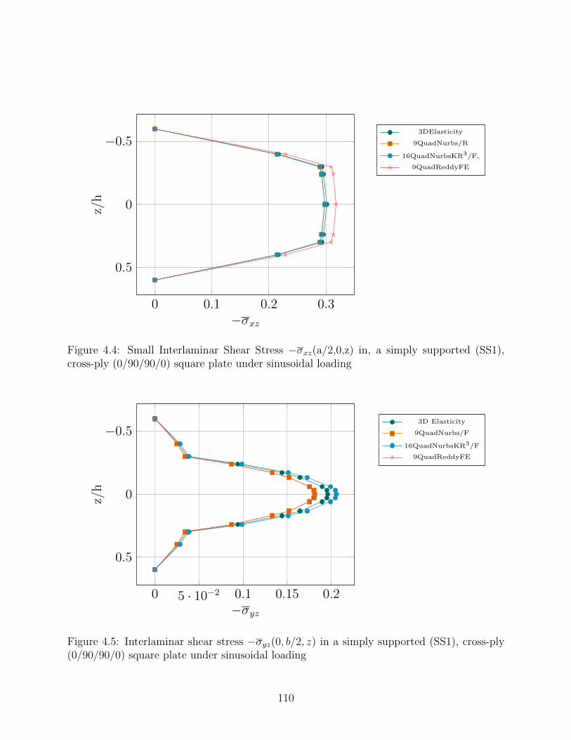
0 0.1 0.2 0.3
−0.5
0
0.5
−σxz
z/h
3DElasticity
9QuadNurbs/R
16QuadNurbsKR3/F,
9QuadReddyFE
Figure 4.4: Small Interlaminar Shear Stress −σxz(a/2,0,z) in, a simply supported (SS1),cross-ply (0/90/90/0) square plate under sinusoidal loading
0 5 · 10−2 0.1 0.15 0.2
−0.5
0
0.5
−σyz
z/h
3D Elasticity
9QuadNurbs/F
16QuadNurbsKR3/F
9QuadReddyFE
Figure 4.5: Interlaminar shear stress −σyz(0, b/2, z) in a simply supported (SS1), cross-ply(0/90/90/0) square plate under sinusoidal loading
110

mesh and two Gauss integration schemes i.e. 3× 3 and 4× 4, are used.
Interlaminar stresses are computed from direct integration of 3D equilibrium equations, with-
out any recovery procedure. Computed stresses are compared with 3D elasticity solutionPagano,
Byun and Kapania(7 × 7 mesh of 9 node quadratic Lagrange element with stress recovery
procedure) and 4Q8Reddy/FE (4× 4 mesh of 8 node quadratic Lagrange element). Tables
4.2, 4.3, 4.4 provide the comparison of in-plane and interlaminar stresses with 3D elasticity
solution, Byun and Kapania’s and Reddy’s results.
Stresses are found to be in an excellent agreement with 3D elasticity solution for at least one
of the elements in the family of k-refined quadratic Nurbs elements when compared with 3D
elasticity solution and Byun and Kapania’s results. However, to obtain the most accurate
interlaminar stresses, a single knot in the knot vector of a particular element of the family
of k-refined quadratic Nurbs elements, for which the most accurate interlaminar stress is
obtained, is replaced by a new knot at a slightly perturbed position. This procedure
produces the most accurate interlaminar stresses which are almost exact to 3D elasticity
solution. This new knot seems to produce most smoothed in-plane stress gradients and
thus, interlaminar stresses. This trend is seen for all the length to thickness ratios and for
both integration schemes. In Tables 4.2, 4.3, 4.4, these stress values are provided with the
new knot location and the knot location are shown as superscript.
111
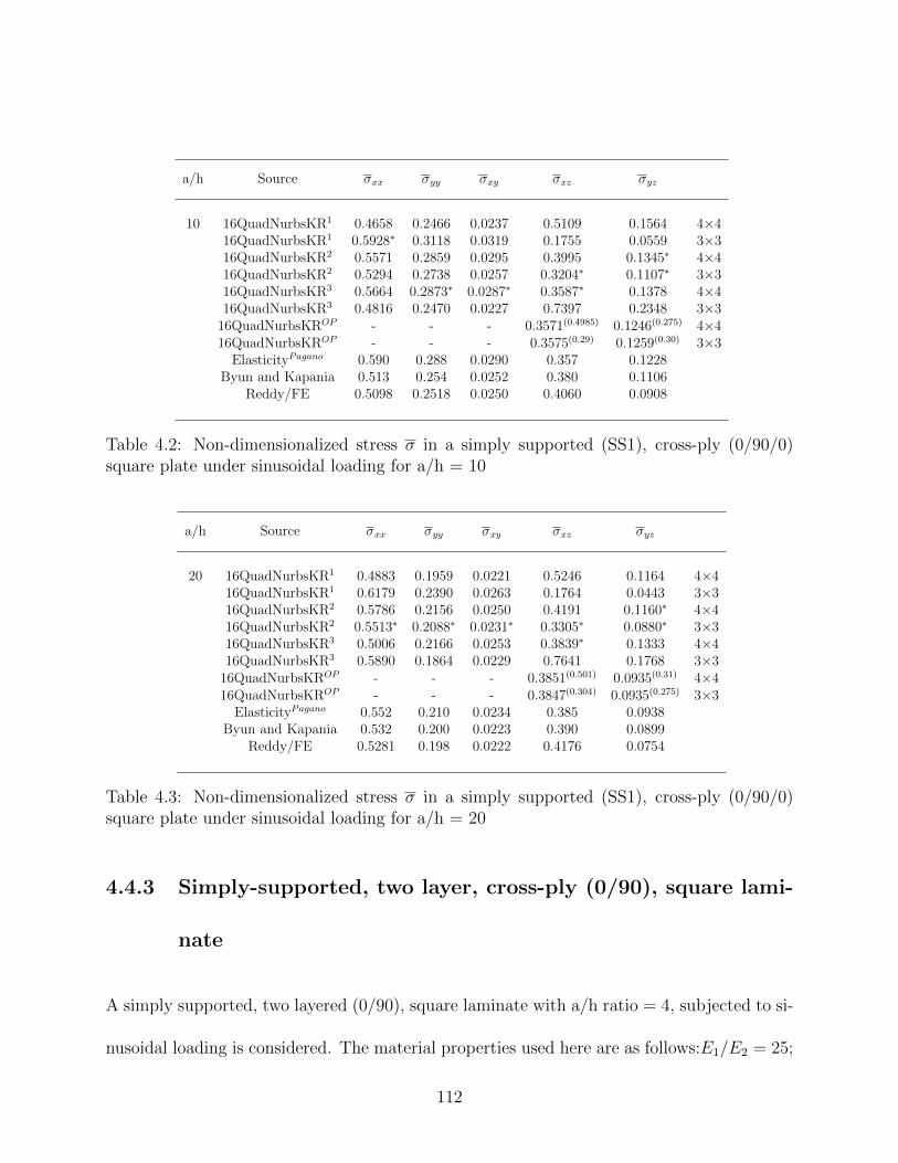
a/h Source σxx σyy σxy σxz σyz
10 16QuadNurbsKR1 0.4658 0.2466 0.0237 0.5109 0.1564 4×416QuadNurbsKR1 0.5928∗ 0.3118 0.0319 0.1755 0.0559 3×316QuadNurbsKR2 0.5571 0.2859 0.0295 0.3995 0.1345∗ 4×416QuadNurbsKR2 0.5294 0.2738 0.0257 0.3204∗ 0.1107∗ 3×316QuadNurbsKR3 0.5664 0.2873∗ 0.0287∗ 0.3587∗ 0.1378 4×416QuadNurbsKR3 0.4816 0.2470 0.0227 0.7397 0.2348 3×3
16QuadNurbsKROP - - - 0.3571(0.4985) 0.1246(0.275) 4×416QuadNurbsKROP - - - 0.3575(0.29) 0.1259(0.30) 3×3
ElasticityPagano 0.590 0.288 0.0290 0.357 0.1228Byun and Kapania 0.513 0.254 0.0252 0.380 0.1106
Reddy/FE 0.5098 0.2518 0.0250 0.4060 0.0908
Table 4.2: Non-dimensionalized stress σ in a simply supported (SS1), cross-ply (0/90/0)square plate under sinusoidal loading for a/h = 10
a/h Source σxx σyy σxy σxz σyz
20 16QuadNurbsKR1 0.4883 0.1959 0.0221 0.5246 0.1164 4×416QuadNurbsKR1 0.6179 0.2390 0.0263 0.1764 0.0443 3×316QuadNurbsKR2 0.5786 0.2156 0.0250 0.4191 0.1160∗ 4×416QuadNurbsKR2 0.5513∗ 0.2088∗ 0.0231∗ 0.3305∗ 0.0880∗ 3×316QuadNurbsKR3 0.5006 0.2166 0.0253 0.3839∗ 0.1333 4×416QuadNurbsKR3 0.5890 0.1864 0.0229 0.7641 0.1768 3×3
16QuadNurbsKROP - - - 0.3851(0.501) 0.0935(0.31) 4×416QuadNurbsKROP - - - 0.3847(0.304) 0.0935(0.275) 3×3
ElasticityPagano 0.552 0.210 0.0234 0.385 0.0938Byun and Kapania 0.532 0.200 0.0223 0.390 0.0899
Reddy/FE 0.5281 0.198 0.0222 0.4176 0.0754
Table 4.3: Non-dimensionalized stress σ in a simply supported (SS1), cross-ply (0/90/0)square plate under sinusoidal loading for a/h = 20
4.4.3 Simply-supported, two layer, cross-ply (0/90), square lami-
nate
A simply supported, two layered (0/90), square laminate with a/h ratio = 4, subjected to si-
nusoidal loading is considered. The material properties used here are as follows:E1/E2 = 25;
112
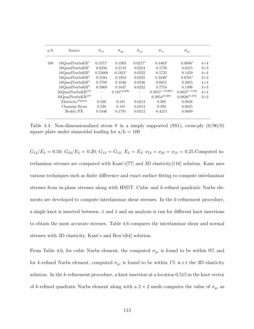
a/h Source σxx σyy σxy σxz σyz
100 16QuadNurbsKR1 0.5371∗ 0.1903 0.0217∗ 0.4463∗ 0.0886∗ 4×416QuadNurbsKR1 0.6256 0.2118 0.0224 0.1750 0.0415 3×316QuadNurbsKR2 0.55668 0.1821∗ 0.0232 0.5722 0.1459 4×416QuadNurbsKR2 0.5594 0.1853 0.0225 0.3346∗ 0.0781∗ 3×316QuadNurbsKR3 0.5788 0.1846 0.0246 0.6651 0.2055 4×416QuadNurbsKR3 0.5069 0.1647 0.0242 0.7754 0.1496 3×3
16QuadNurbsKROP - 0.181(0.268) - 0.3957(−0.0407) 0.0827(−0.02) 4×416QuadNurbsKROP - - - 0.3954(0.309) 0.0826(0.275) 3×3
ElasticityPagano 0.539 0.181 0.0213 0.395 0.0828Chansup Byun 0.539 0.181 0.0213 0.394 0.0825
Reddy/FE 0.5346 0.1791 0.0212 0.4215 0.0699
Table 4.4: Non-dimensionalized stress σ in a simply supported (SS1), cross-ply (0/90/0)square plate under sinusoidal loading for a/h = 100
G12/E2 = 0.50; G23/E2 = 0.20; G13 = G12; E2 = E3; ν12 = ν23 = ν13 = 0.25.Computed in-
terlaminar stresses are compared with Kant’s[77] and 3D elasticity[116] solution. Kant uses
various techniques such as finite difference and exact surface fitting to compute interlaminar
stresses from in-plane stresses along with HSDT. Cubic and k-refined quadratic Nurbs ele-
ments are developed to compute interlaminar shear stresses. In the k-refinement procedure,
a single knot is inserted between -1 and 1 and an analysis is run for different knot insertions
to obtain the most accurate stresses. Table 4.6 compares the interlaminar shear and normal
stresses with 3D elasticity, Kant’s and Ren’s[64] solution.
From Table 4.6, for cubic Nurbs element, the computed σyz is found to be within 9% and
for k-refined Nurbs element, computed σyz is found to be within 1% w.r.t the 3D elasticity
solution. In the k-refinement procedure, a knot insertion at a location 0.515 in the knot vector
of k-refined quadratic Nurbs element along with a 2× 2 mesh computes the value of σyz as
113

0.3161 when compared to the value of σyz 0.3188 obtained from the 3D elasticity’s solution,
0.319233 obtained from Kant’s HOST11(16N)(direct integration(DI)) element, which is a
cubic, 16 node element with 11 degrees of freedom per node, and 0.32580 computed from
Ren’s higher order shear deformation theory model. Figure 4.6 shows the comparison
of through the thickness distribution of σxz with 3D elasticity solution. Similarly, σyz is
computed using cubic and quadratic Nurbs element. Figure 4.7 shows the comparison of
interlaminar shear stress, σyz, with the 3D elasticity solution.
However, σzz requires calculation of third-order displacement derivatives and thus, require
higher order polynomial approximation of solution space. Cubic and quartic Nurbs elements
are constructed for computing σzz. From Table 4.6, it is observed that Nurbs elements
produce better estimate of through thickness distribution of σzz as compared to Kant’s
solution. The k-refinement procedure seems to enhance the smoothness of strain gradients
and thus, 3D elasticity equivalent interlaminar normal stresses are obtained for various single
knot insertion values. Figure 4.8 shows the comparison of through the thickness distribution
of interlaminar normal stress with the 3D elasticity and Kant’s solutions.
4.4.4 Simply supported, anti-symmetric, angle-ply, square lami-
nate
A simply supported (SS2), 2 and 10 layered, (45 -45), anti-symmetric square laminate for
various a/h ratios, subjected to sinusoidal loading is analyzed here. The material properties
114

0 0.1 0.2 0.3
−0.6
−0.4
−0.2
0
0.2
0.4
0.6
−σxz
z/h
3D Elasticity
16quadNurbsKR3
16CubicNurbsKR
Figure 4.6: Interlaminar Shear Stress −σxz(a/2, 0, z) in a simply supported (SS1), cross-ply(0/90) square plate under sinusoidal loading
0 0.1 0.2 0.3
−0.6
−0.4
−0.2
0
0.2
0.4
0.6
−σyz
z/h
3D Elasticity
16CubicNurbs
16quadNurbsKR3
Figure 4.7: Interlaminar Shear Stress −σyz(0, b/2, z) in a simply supported (SS1), cross-ply(0/90) square plate under sinusoidal loading
115
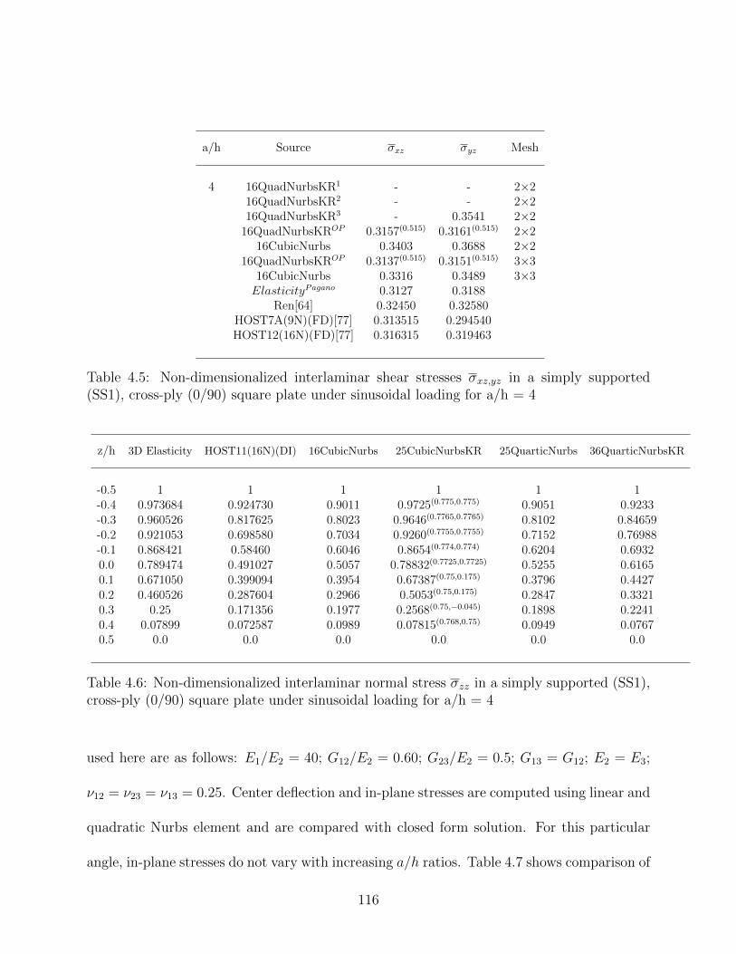
a/h Source σxz σyz Mesh
4 16QuadNurbsKR1 - - 2×216QuadNurbsKR2 - - 2×216QuadNurbsKR3 - 0.3541 2×2
16QuadNurbsKROP 0.3157(0.515) 0.3161(0.515) 2×216CubicNurbs 0.3403 0.3688 2×2
16QuadNurbsKROP 0.3137(0.515) 0.3151(0.515) 3×316CubicNurbs 0.3316 0.3489 3×3ElasticityPagano 0.3127 0.3188
Ren[64] 0.32450 0.32580HOST7A(9N)(FD)[77] 0.313515 0.294540HOST12(16N)(FD)[77] 0.316315 0.319463
Table 4.5: Non-dimensionalized interlaminar shear stresses σxz,yz in a simply supported(SS1), cross-ply (0/90) square plate under sinusoidal loading for a/h = 4
z/h 3D Elasticity HOST11(16N)(DI) 16CubicNurbs 25CubicNurbsKR 25QuarticNurbs 36QuarticNurbsKR
-0.5 1 1 1 1 1 1-0.4 0.973684 0.924730 0.9011 0.9725(0.775,0.775) 0.9051 0.9233-0.3 0.960526 0.817625 0.8023 0.9646(0.7765,0.7765) 0.8102 0.84659-0.2 0.921053 0.698580 0.7034 0.9260(0.7755,0.7755) 0.7152 0.76988-0.1 0.868421 0.58460 0.6046 0.8654(0.774,0.774) 0.6204 0.69320.0 0.789474 0.491027 0.5057 0.78832(0.7725,0.7725) 0.5255 0.61650.1 0.671050 0.399094 0.3954 0.67387(0.75,0.175) 0.3796 0.44270.2 0.460526 0.287604 0.2966 0.5053(0.75,0.175) 0.2847 0.33210.3 0.25 0.171356 0.1977 0.2568(0.75,−0.045) 0.1898 0.22410.4 0.07899 0.072587 0.0989 0.07815(0.768,0.75) 0.0949 0.07670.5 0.0 0.0 0.0 0.0 0.0 0.0
Table 4.6: Non-dimensionalized interlaminar normal stress σzz in a simply supported (SS1),cross-ply (0/90) square plate under sinusoidal loading for a/h = 4
used here are as follows: E1/E2 = 40; G12/E2 = 0.60; G23/E2 = 0.5; G13 = G12; E2 = E3;
ν12 = ν23 = ν13 = 0.25. Center deflection and in-plane stresses are computed using linear and
quadratic Nurbs element and are compared with closed form solution. For this particular
angle, in-plane stresses do not vary with increasing a/h ratios. Table 4.7 shows comparison of
116
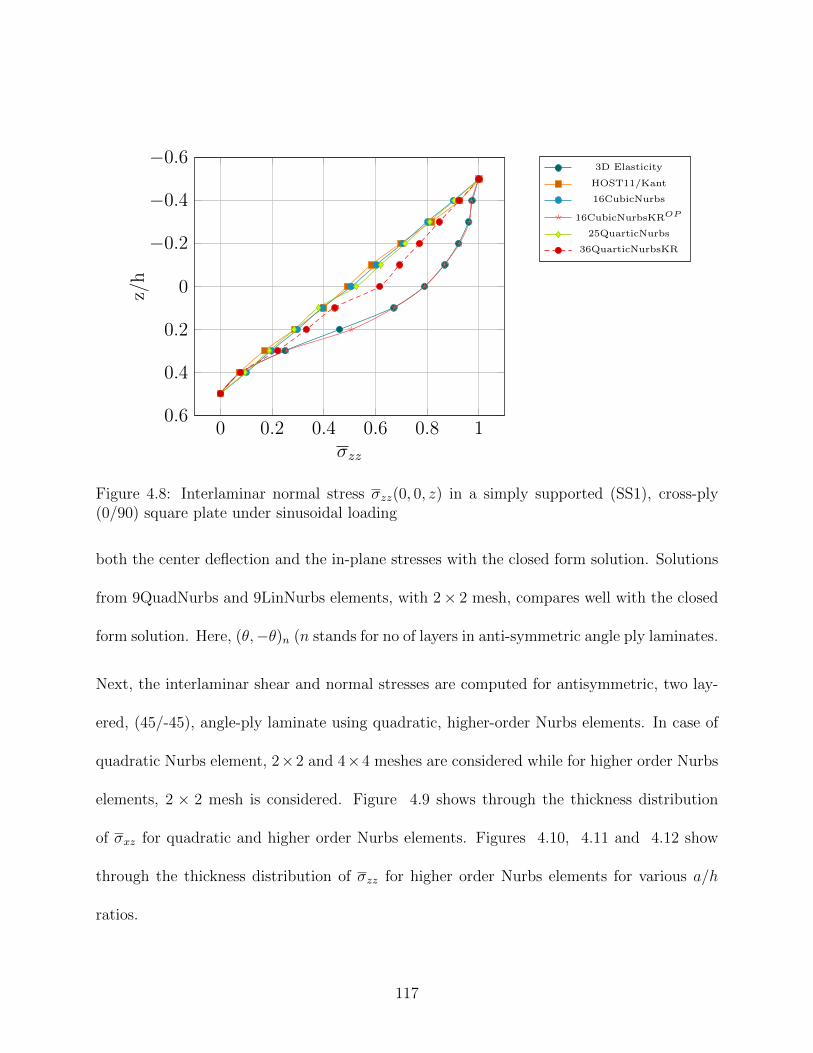
0 0.2 0.4 0.6 0.8 1
−0.6
−0.4
−0.2
0
0.2
0.4
0.6
σzz
z/h
3D Elasticity
HOST11/Kant
16CubicNurbs
16CubicNurbsKROP
25QuarticNurbs
36QuarticNurbsKR
Figure 4.8: Interlaminar normal stress σzz(0, 0, z) in a simply supported (SS1), cross-ply(0/90) square plate under sinusoidal loading
both the center deflection and the in-plane stresses with the closed form solution. Solutions
from 9QuadNurbs and 9LinNurbs elements, with 2× 2 mesh, compares well with the closed
form solution. Here, (θ,−θ)n (n stands for no of layers in anti-symmetric angle ply laminates.
Next, the interlaminar shear and normal stresses are computed for antisymmetric, two lay-
ered, (45/-45), angle-ply laminate using quadratic, higher-order Nurbs elements. In case of
quadratic Nurbs element, 2×2 and 4×4 meshes are considered while for higher order Nurbs
elements, 2 × 2 mesh is considered. Figure 4.9 shows through the thickness distribution
of σxz for quadratic and higher order Nurbs elements. Figures 4.10, 4.11 and 4.12 show
through the thickness distribution of σzz for higher order Nurbs elements for various a/h
ratios.
117

−0.1−5 · 10−2 0 5 · 10−2 0.1
−0.4
−0.2
0
0.2
0.4
−σxz
z/h
9QuadNurbs,(3× 3)
16CubicNurbs,(2× 2)
25QuarticNurbs,(2× 2)
36QuinticNurbs,(2× 2)
Figure 4.9: Through the thickness distribution of interlaminar shear stress, −σxz(a/2, 0, z),in a simply supported (SS2), anti-symmetric (45/-45) square laminated plate, a/h=4
0 0.2 0.4 0.6 0.8 1
−0.4
−0.2
0
0.2
0.4
σzz
z/h
16CubicNurbs
25QuarticNurbs
36QuinticNurbs
Figure 4.10: Through the thickness distribution of interlaminar shear stress, σzz(0, 0, z), ina simply supported (SS2), antisymmetric (45/-45) square laminated plate, a/h=4
118
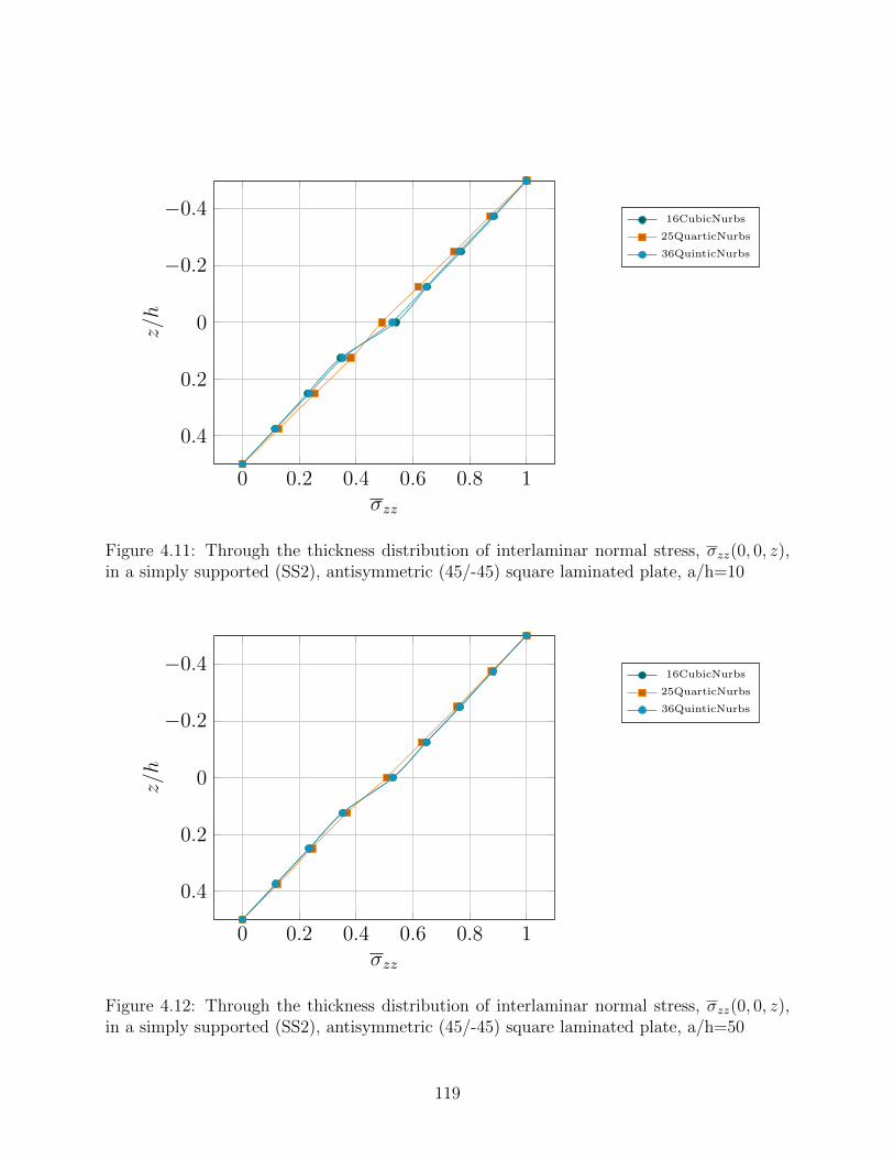
0 0.2 0.4 0.6 0.8 1
−0.4
−0.2
0
0.2
0.4
σzz
z/h
16CubicNurbs
25QuarticNurbs
36QuinticNurbs
Figure 4.11: Through the thickness distribution of interlaminar normal stress, σzz(0, 0, z),in a simply supported (SS2), antisymmetric (45/-45) square laminated plate, a/h=10
0 0.2 0.4 0.6 0.8 1
−0.4
−0.2
0
0.2
0.4
σzz
z/h
16CubicNurbs
25QuarticNurbs
36QuinticNurbs
Figure 4.12: Through the thickness distribution of interlaminar normal stress, σzz(0, 0, z),in a simply supported (SS2), antisymmetric (45/-45) square laminated plate, a/h=50
119

a/h Source w ∗ 102 w ∗ 102 σxx σxy(n = 2) (n = 10) (n = 10) (n = 10)
4 9QuadNurbs 1.1850 0.8645 0.14377 0.140169LinNurbs 1.18038 0.8654 0.1386 0.1349
Closed Form 1.1576 0.8450 0.1430 0.1392
10 9QuadNurbs 0.5907 0.27098 0.14377 0.14029LinNurbs 0.58395 0.2690 0.1386 0.1350
Closed Form 0.5773 0.2647 0.1430 0.1392
20 9QuadNurbs 0.5053 0.1860 0.14379 0.14039LinNurbs 0.4987 0.1838 0.13865 0.1350
Closed Form 0.4944 0.1818 0.1430 0.1392
100 9QuadNurbs 0.4757 0.1565 0.14379 0.14039LinNurbs 0.4713 0.1581 0.13883 0.135368
Closed Form 0.4678 0.1553 0.1430 0.1392
Table 4.7: Non-dimensionalized displacement and in-plane stresses in a simply supported(SS2), cross-ply (45/-45) square plate under sinusoidal loading
4.4.5 Simply-supported, sandwich plate
A simply supported (SS1), sandwich plate subjected to sinusoidal distributed transverse
loading is analyzed here. The face sheet’s material (orthotropic) properties used here are as
follows: E1 = 25E2; E2 = 1E6; G12 = 0.50E2; G23 = 0.2; G13 = G12; ν12 = ν13 = 0.25 the
core material properties are as follows, E1 = E2 = 1e6; G13 = G23 = 0.06E6; G12 = 0.16E6;
and ν12 = 0.25. Each face sheet is assumed to have one tenth of the total thickness of the
sandwich plate. In-plane stresses are computed using 9QuadNurbs and 9LinNurbs elements
with 2× 2 mesh and 2× 2 and 3× 3 Gauss integration schemes (GIS). Linear Nurbs element
with 0 as single knot insertion computes in-plane stresses which are very close to 3D
elasticity solution. While the 9QuadNurbs element behaves similar to 9QuadLagrange finite
120

element with slightly better in-plane stresses. For example, 9LinNurbs element with 0 as
single knot insertion and with 3×3 Gauss integration scheme computes value of σxx(0, 0, h/2)
as 1.5896 as compared to 1.556 computed using the 3D elasticity solution, 0.8918 computed
using Reddy’s 4 × 4 mesh of 9QuadLagrange finite element and 0.9522 computed using
9QuadNurbs element with 2 × 2 mesh and 3 × 3 Gauss integration scheme. Similar results
are obtained for σyy(0, 0, h/2) as well. However, in case of σxy(a/2, b/2,−h/2), LinearNurbs
element with knot insertion at 0.2 and with 3× 3 Gauss integration scheme produces the
3D elasticity equivalent in-plane shear stress.
Interlaminar shear stresses are computed using 9QuadNurbs, 16QuadNurbsKR and 16Cu-
bicNurbs elements with 2 × 2 mesh and 3 × 3 and 4 × 4 Gauss integration schemes. The
k-refined Nurbs element produces interlaminar shear stresses which are closer to the 3D elas-
ticity solution than the 9QuadNurbs and the 16CubicNurbs elements. Table 4.8 shows the
comparison of in-plane and interlaminar shear stresses with 3D elasticity and 4× 4 mesh of
the 9QuadLagrange finite element.
4.5 Conclusions
This chapter describes the development of Nurbs post-processor for computation of inter-
laminar stresses in laminated composite and sandwich plates. First-order, shear-deformable
laminate composite plate theory is utilized in deriving the governing equations using a vari-
ational formulation. Linear, quadratic, higher order and k-refined Nurbs elements are con-
121

a/h Source σxx σyy σxy σxz σyz GIS
4 9LinNurbs 0.8714(0) 0.15587(0) 0.1157(−0.5) - - 2×29LinNurbs 1.5896(0) 0.2651(0) 0.14397(0.2) - 3×39QuadNurbs 0.9167 0.16191 0.0939 0.26094 0.0682 2×29QuadNurbs 0.9522 0.1679 0.0977 0.2645 0.0683 3×3
16QuadNurbsKR - - - 0.2396(0.25) 0.1078(0.4) 3×316QuadNurbsKR - - - 0.2343(0.45) 0.1078(0.625) 4×416CubicNurbsKR - - - 0.2929 0.0781 3×316CubicNurbsKR - - - 0.2127 0.0789 4×49QuadFEM/Reddy 0.8918 0.1551 0.0901 0.2808 0.0746 3×3
3D Elasticity 1.556 0.2595 0.1481 0.239 0.1072
Table 4.8: Non-dimensionalized in-plane and interlaminar shear stresses in a simply sup-ported (SS1), sandwich square plate under sinusoidal loading
structed. Lagrange finite element suffers from higher- order strain gradient oscillations due
to Gibbs phenomenon and require alternative stress recovery procedures. In this chapter,
a Nurbs based post-processor is developed which computes interlaminar shear and normal
stresses directly from higher order gradients of Nurbs basis in a single step procedure. Nu-
merical examples tested include symmetric, anti-symmetric composite and sandwich plates.
In addition, it is observed that smoothed linear Nurbs with knot insertion at optimal point
and k-refined Nurbs elements compute 3D elasticity equivalent in-plane and interlaminar
stresses for coarsest meshes.
122

Chapter 5
Stress analysis of Composite Plate
with Hole using Nurbs Isogeometric
Finite Element Analysis
This chapter presents the stress analysis of laminated composite plate with a hole using
Nurbs Isogeometric finite element analysis, especifically, developed to study stress concen-
tration problem. Geometry is modeled exactly in Isogeometric framework and iso-parametric
finite element representation is invoked for field variable defination. The h-refinement pro-
cess is performed internally by inserting a single knot in the knot vector and corresponding
control net is obtained from the algorithm. The control net forms the scaffold over the
physical mesh and is interpolatory only at the end points. Isotropic, (90/0)s and (−45/45)s
123

laminates are studied under remote loading and one-forth model is considered due to sym-
metry. Convergence study is performed for various Isogeometric meshes. The streses are
found to be in good agreement with the literature.
5.1 Plate with a Circular Hole Nurbs geometry
This subsection describes the generation of circular hole plate geometry, by construction of
Nurbs basis and Nurbs surface generation. A h-refinement process is then described which
is used for subsequent mesh refinements.
5.1.1 B-spline Basis
A knot vector in one dimension is a set of co-ordinates in the parametric space,
Ξ = ξ1, ξ2, ......, ξn+p+1, where ξi is the ith knot, i is the knot index where i = 1, 2, ....., n+
p + 1, p is the order of the polynomial and n is the number of basis functions. The order
of the polynomial, p = 0, 1, 2, 3...., refers to the constant, linear, quadratic, cubic piecewise
polynomials, respectively. If more than one knot is located at the same parametric co-
ordinate, these are termed as repeated knots. In case of the open knot vector, first and
last knots are repeated p + 1 times. Basis function formed using the open knot vector are
interpolatory at the beginning and end of the parametric space interval, i.e. [ξ1, ξn+p+1].
This distinguishes the knots from the nodes in the finite element analysis as all the nodes
are interpolatory. As a starting point, B-spline basis functions are defined recursively using
124

Cox-Deboor algorithm, starting with piecewise constants (p = 0).
Npi (ξ) =
1 if ξi ≤ ξ < ξi+1,
0 otherwise
(5.1)
And, subsequently, basis functions for orders p = 1, 2, 3, ....., are defined as follows,
Npi (ξ) =
ξ − ξiξi+p − ξi
Np−1i (ξ) +
ξi+p+1 − ξξi+p+1 − ξi+1
Np−1i+1 (ξ) (5.2)
5.1.2 Non-uniform Rational B-spline (Nurbs) Basis
2D Nurbs basis are formed by tensor product of B-spline basis in ξ and η direction and
using projective weights associated with the control points. Rational basis functions are
very similar to B-spline basis and derive the continuity and support for the function from
the knot vector. Also, Nurbs basis form a partition of unity and are pointwise non-negative.
These properties result in a strong convex hull property. Rational basis are formed as follows,
Rp,qi,j (ξ, η) =
Npi (ξ)M q
j (η)Wi,j∑CPwi=1
∑CPui=1 Np
i (ξ)M qj (η)Wi,j
≈ Rpk (5.3)
Nurbs surface is defined as,
S(x, y) =CPw∑j=1
CPu∑i=1
Rp,qi,j (ξ, η)Bi,j (5.4)
125

where Npi (ξ) and M q
j (η) are the B-spline basis in ξ and η direction and Rp,qi,j denotes a 2D
Nurbs basis function. CPw and CPu are the number of control points in ξ and η directions
and nCP = CPu × CPw is the total number of control points per element. Wi,js are the
weights associated with the control points, Bi,j and weights are the vertical coordinates of
the corresponding control points. Here, weights, W s considered are equal to one.
5.1.3 h-refinement: Knot Insertion
h-refinement is the process of single knot insertion in the knot vector. Given a knot
vector ξ = ξ1, ξ2, ......, ξn+p+1, let ξ− > [ξk, ξk+1] be a desired new knot. The new
n + 1 basis functions are formed recursively and new knot vector generated is as follows;
ξ =ξ1, ξ2, ...ξk, ξ, ξk+1...., ξn+p+1
. The new n + 1 control points,
B1, B2, .......Bn+1
are
formed from the original control points, B1, B2, ......., Bn by
Bi = αiBi + (1− αi) ∗Bi−1 (5.5)
where
αi =
1 1 ≤ ik − p
ξi−ξiξi+p−ξi k − p+ 1 ≤ ik
0 k + 1 ≤ i ≤ n+ p+ 2
(5.6)
Continuity of the curve is preserved by choosing the control points using above equations.
126
5.1.4 Circular hole plate geometry
A plate with a circular hole geometry is modeled here in Isogeometric framework. one-eightth
of plate with open-hole is modeled due to symmetry. The h and p-refinement processes are
applied for increasing mesh density. The coarsest mesh is defined by the knot vectors,
ξ = 0, 0, 0, 0.5, 1, 1, 1 and η = 0, 0, 0, 1, 1, 1. Figures 5.1(a) and (b) show the physical
meshes and the control net for the plate with a circular hole. Two control points on the
upper left corner creates the corner for the plate. Figures 5.2(a) and (b) show the parametric
domain and the index space respectively. Exact geometry is represented by two elements
(Mesh0). Figures 5.3(a)− (d) show various h-refined physical meshes. Physical mesh shown
in 5.3(a) consists of 8 elements and 120 linear equations (Mesh2), mesh in 5.3(b) consist
of 32elements and 300 equations (Mesh3), mesh in 5.3(c) consists of 128 elements and 900
equations (Mesh4) and mesh in 5.3(d) consists of 512 elements and 3060 linear equations
(Mesh5) and Mesh6 consists of 2048 elements and 11220 equations.
5.2 Numerical Validation
Stress concentration plays an important role in the design of layered structures. A plate
with a circular hole is an important concentration problem under far-field tension load-
ing. Symmetry boundary condition is applied at quarter symmetry. Isotropic, (0, 90)s and
(−45, 45)s laminates are considered for analysis. In-plane stresses are computed at the free
127

Figure 5.1: 2 element physical mesh and control net for plate with circular hole geometry
edge boundary and mesh convergence study is presented.
5.2.1 Stress analysis of isotropic plate with open hole
This example studies the circular hole problem in infinite plate under uniaxial loading.
Material considered is homogeneous, elastic and isotropic and the properties are as follows;
E1 = E2; G12 = 0.5E2 = G23 = G13; ν12 = 0.3. Normalized hoop-stress is computed
along the hole’s free edge under remote tensle loading. Table 5.1 shows the hoop stress
distribution for 900 angle around the hole. Maximum hoop stress (σθθ/σ0) is obtained at
128

Figure 5.2: Two element parametric mesh and index space for plate with a circular holegeometry
hole’s free edge and stress concentration factor is found to be 3 which is in agreement with
analytical solution. Next, convergence study for increased mesh density is presented. With
Mesh2, Mesh3 and Mesh4, stresses are found to converge within 1% difference as compared
with previous mesh.
129

Source σθθ/σ0(900)
NurbsIso0 3.0334
NurbsIso2 2.9978
NurbsIso3 3.0226
NurbsIso4 3.0226
Analytical 3.0
Table 5.1: Stress convergence test for σθθ/σ0 at 90 degree angle i.e. hole edge in the mid-planeof isotropic plate
5.2.2 Stress analysis of (90, 0)s laminated composite plate with
open hole
Material considered is homogeneous, elastic and orthotropic. The properties are as follows;
E1 = 138 GPa; E2 = 14 GPa; G12 = 5.86 GPa; G23 = 3.43 GPa; G13 = G12; ν12 =
ν13 = 0.3. Normalized hoop-stress is computed along the hole-edge in the middle of 900 (z =
−3h/8) and 00 (z = −h/8) plies. Figures 5.6 and 5.7 shows the hoop stress distribution
for various angles around the hole and convergence study with increasing mesh density is
presented. With Mesh3 and Mesh4, stresses are found to converge within 3− 5% difference
as compared with previous mesh. Stress concentration increases with the angle along the
circumference and reaches extremum at 900 along the hole’s other edge.
For validation purposes, analysis was carried out with different orthotropic material prop-
130
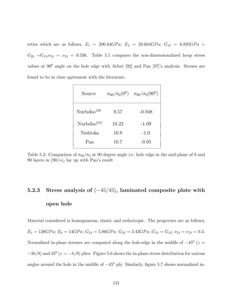
erties which are as follows, E1 = 206.84GPa; E2 = 20.684GPa; G12 = 6.895GPa =
G23 =G13;ν12 = ν13 = 0.336. Table 5.1 compares the non-dimensionalized hoop stress
values at 900 angle on the hole edge with Atluri [92] and Pan [97]’s analysis. Streses are
found to be in close agreement with the literature.
Source σθθ/σ0(00) σθθ/σ0(900)
NurbsIso128 9.57 -0.948
NurbsIso512 10.22 -1.09
Nishioka 10.8 -1.0
Pan 10.7 -0.95
Table 5.2: Comparison of σθθ/σ0 at 90 degree angle i.e. hole edge in the mid-plane of 0 and90 layers in (90/s)s lay up with Pan’s result
5.2.3 Stress analysis of (−45/45)s laminated composite plate with
open hole
Material considered is homogeneous, elastic and orthotropic. The properties are as follows;
E1 = 138GPa; E2 = 14GPa; G12 = 5.86GPa; G23 = 3.43GPa; G13 = G12; ν12 = ν13 = 0.3.
Normalized in-plane stresses are computed along the hole-edge in the middle of −450 (z =
−3h/8) and 450 (z = −h/8) plies. Figure 5.6 shows the in-plane stress distribution for various
angles around the hole in the middle of −450 ply. Similarly, figure 5.7 shows normalized in-
131

plane stress distribution at various angles along the hole edge in the middle of 450 ply. These
stresses are plotted using Mesh5 which shows stress convergence within 2 − 3% difference
from one level less refined mesh.
5.3 Conclusions
This research presents the stress analysis around a hole’s free edge in a laminated com-
posite plate using Nurbs Isogeometric finite element, specifically developed to study stress
concentration problem. Geometry is modeled exactly in Isogeometric framework and iso-
parametric finite element representation is invoked for solution space. Various refined Iso-
geometric meshes are generated for convergence study using the h-refinement process. The
h-refinement process is performed internally by inserting a single knot in the knot vector
and the corresponding control net is obtained from the algorithm. The control net forms
the scaffold over the physical mesh and is interpolatory only at the end points. Exactly the
same basis functions are used for field variable representation as are used for geometric rep-
resentation. Isotropic, (90/0)s and (−45/45)s laminates are studied under remote in-plane
loading and one-quater of the model is considered due to symmetry. In isotropic case, all the
meshes converges to the analytical solution. For other cases, convergence study is performed
for various Isogeometric meshes and good agreement is found with literature as well.
132
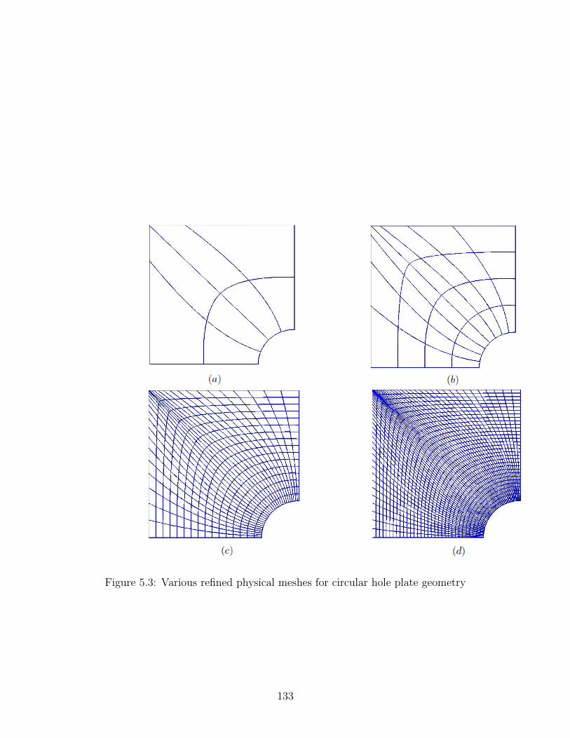
Figure 5.3: Various refined physical meshes for circular hole plate geometry
133

0 20 40 60 80 100
0
2
4
6
8
10
θ
σθθ/σ
0
Mesh2
Mesh3
Mesh4
Figure 5.4: Variation of σθθ/σ0 around the hole edge in the middle of 0 layer in (0/90)scomposite plate with a circular hole
0 20 40 60 80 100
−4
−2
0
2
θ
σθθ/σ
0
Mesh2
Mesh3
Mesh4
Figure 5.5: Variation of σθθ/σ0 around the hole edge in the middle of 90 layer in (0/90)scomposite plate with a circular hole
134

0 20 40 60 80 100
−2
0
2
θ
σ/σ
0
σθθ/σ0
σrθ/σ0
σrr/σ0
Figure 5.6: Variation of stresses around the hole edge in the middle of -45 layer in (−45/45)slaminate at refinement level 5
0 20 40 60 80 100
−2
0
2
4
6
θ
σ/σ
0
σθθ/σ0
σrθ/σ0
σrr/σ0
Figure 5.7: Variation of normalised stresses around the hole edge in the middle of 45 layerin (−45/45)s laminate with refinement level 5
135

Chapter 6
Free Vibration and Linear Dynamics
Analysis
This chapter describes the development of Nurbs Isogeometric finite element analysis code
for free vibration and linear dynamics analysis of composite plates. First-order, shear-
deformable laminate composite plate theory is utilized in deriving the governing equations
using a variational formulation. Linear, quadratic, higher order and k-refined Nurbs ele-
ments are constructed and numerical validation is performed for orthotropic and laminated
composite plates. Different ply to thickness ratios, modulus ratios and ply-angles are con-
sidered.
136

6.1 First-order shear deformation plate theory for Lam-
inated Composite Plates
6.1.1 Governing Equations
The origin of material coordinate system is considered to be the mid-plane of the laminate
and Kirchhoff assumption that the transverse normal remain perpendicular to the mid-
surface after deformation is relaxed. However, transverse strain, εz, and out-of plane normal
stress, σz are considered negeligible. Layers are assumed to be perfectly bonded. Figure 6.1
shows the coordinate system and layer numbering of a laminated composite plate. Figure 6.2
shows the undeformed and deformed configuration of first order shear-deformable laminated
composite plate. The displacement field is defined as,
u(x, y, z, t) = u0(x, y, t) + zφx(x, y, t)
v(x, y, z, t) = v0(x, y, t) + zφy(x, y, t) (6.1)
w(x, y, z, t) = w0(x, y, t)
where u0, v0, w0, are the displacement along the x, y and z-axis and φx, φy are the rotation
of transverse normal of the mid-plane about the y and x-axis respectively and t is the time
variable.
137

x
yz
kh/2
h/2
Figure 6.1: Coordinate system and layer numbering used for a laminate plate
Figure 6.2: Undeformed and deformed configuration of first order shear-deformable plate
138

Total in-plane strain ε is decomposed into membrane and bending strains.
ε = εm + zεb (6.2)
εm, the membrane strain can be written as follows,
εm =
εmx
εmy
γmxy
=
∂u0∂x
∂v0∂y
∂u0∂y
+ ∂v0∂x
(6.3)
εb, the bending strain can be written as follows,
εb =
εbx
εby
γbxy
=
∂φy∂y
∂φy∂y
∂φx∂y
+ ∂φy∂x
(6.4)
The transverse shear strain can be written as follows,
γyz
γxz
=
∂w0
∂x+ φx
∂w0
∂y+ φy
(6.5)
The stress strain relation w.r.t principal material co-ordinate system of a lamina can be
139

written as,
σxx
σyy
σxy
(k)
=
Q11 Q12 Q16
Q12 Q22 Q26
Q16 Q26 Q66
(k)
εxx
εyy
γxy
(6.6)
τyz
τxz
(k)
=
Q44 Q45
Q45 Q55
(k)
γyz
γxz
(6.7)
The equilibrium equations are developed from stress resultants by considering balance of
force and moment on an infinitesimal area of the laminate. The strong form of the governing
equation of motion can, then, be written as,
∂Nxx
∂x+∂Nxy
∂y= I0
∂2wo∂t2
+ I1∂2φx∂t2
∂Nxy
∂x+∂Nyy
∂y= I0
∂2vo∂t2
+ I1∂2φy∂t2
∂Qx
∂x+∂Qy
∂y+ q = I0
∂2w0
∂t2(6.8)
∂Mxx
∂x+∂Mxy
∂y−Qx = I2
∂2φx∂t2
+ I1∂2u0
∂t2
∂Mxy
∂x+∂Myy
∂y−Qy = I2
∂2φy∂t2
+ I1∂2v0
∂t2
where N = Nxx, Nyy, Nxy are the force resultants, M = Mxx,Mxy,Myy are the moment
resultants and Q = Qx, Qy are the shear force resultants. These resultants acting per unit
140
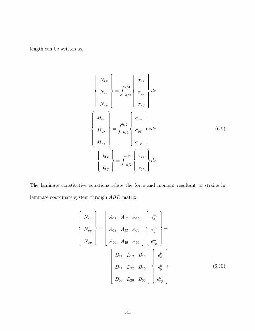
length can be written as,
Nxx
Nyy
Nxy
=∫ h/2
−h/2
σxx
σyy
σxy
dz
Mxx
Myy
Mxy
=∫ h/2
−h/2
σxx
σyy
σxy
zdz (6.9)
Qx
Qy
=∫ h/2
−h/2
τxz
τyz
dz
The laminate constitutive equations relate the force and moment resultant to strains in
laminate coordinate system through ABD matrix.
Nxx
Nyy
Nxy
=
A11 A12 A16
A12 A22 A26
A16 A26 A66
εmx
εmy
εmxy
+
B11 B12 B16
B12 B22 B26
B16 B26 B66
εbx
εby
εbxy
(6.10)
141

Mxx
Myy
Mxy
=
B11 B12 B16
B12 B22 B26
B16 B26 B66
εmx
εmy
εmxy
+
D11 D12 D16
D12 D22 D26
D16 D26 D66
εbx
εby
εbxy
(6.11)
Qy
Qx
= K
A44 A45
A45 A55
γyz
γxz
(6.12)
(Aij, Bij, Dij) =N∑k=1
(Qk
ij (zk+1 − zk) ,1
2Qk
ij
(z2k+1 − z2
k
), (6.13)
1
3Qk
ij
(z3k+1 − z3
k
)
(A44, A45, A55) =∑Nk=1
(Qk
44, Qk
45, Qk
55
)(zk+1 − zk) (6.14)
142

In the ABD matrix, Aij, Bij and Dij terms represent extensional and shear, extensional-
bending coupling and bending stiffness terms and Qkijs are plane-stress reduced stiffness
terms. K is the shear correction factor.
Weak form of the governing equations is obtained by pre-multipying the equation of motion
with δu0, δv0, δw0, δφx and δφy respectively and integrating by parts over the element
domain. Substituting the in-plane force, moment and shear force resultant,
0 =∫
Ωe
(∂δu0
∂xNxx +
∂δu0
∂yNyy + I0δu0
∂2uo∂t2
+ I1δu0∂2φx∂t2
)dxdy
−∮
ΓePxδu0ds
0 =∫
Ωe
(∂δv0
∂xNxy +
∂δv0
∂yNyy + I0δv0
∂2vo∂t2
+ I1δv0∂2φy∂t2
)dxdy
−∮
ΓePyδu0ds
0 =∫
Ωe
[∂δw0
∂xQx +
∂δW0
∂yQy − δw0q + I0δw0
∂2w0
∂t2+
∂δw0
∂x
(Nxx
∂δw0
∂x+ Nxy
∂δw0
∂y
)+∂δw0
∂y
(Nxy
∂δw0
∂x+ Nyy
∂δw0
∂y
)]dxdy −
∮Γe
[(Qx + Nxx
∂δw0
∂x+ Nxy
∂δw0
∂y
)nx +
(Qy + Nxy
∂δw0
∂x
+Nyy∂δw0
∂y
)nyδw0ds
143

(6.16)0 =
∫Ωe
(∂δφx∂x
Mxx +∂δφx∂y
Mxy + δφxQx + I2δφx∂2φx∂t2
+
I1δφx∂2u0
∂t2
)dxdy −
∮ΓeTxδφxds
0 =∫
Ωe
(∂δφy∂x
Mxy +∂δφy∂y
Myy + δφyQy + I2δφy∂2φy∂t2
+
I1δφy∂2v0
∂t2
)dxdy −
∮ΓeTyδφyds
6.2 Linear Nurbs Isogeometric Finite Element Formu-
lation / Dynamics
6.2.1 Finite Element Model
The dependent displacement field variables are approximated by Nurbs basis as follows,
u0(x, y) =nCP∑j=1
ujRj(x(ξ, η), y(ξ, η)), v0(x, y) =nCP∑j=1
vjRj(x(ξ, η), y(ξ, η))
w0(x, y) =nCP∑j=1
wjRj(x(ξ, η), y(ξ, η)) (6.17)
φx(x, y) =nCP∑j=1
φxjRj(x(ξ, η), y(ξ, η)), φy(x, y) =nCP∑j=1
φyjRj(x(ξ, η), y(ξ, η))
where nCP are the number of control points per element and Rj are 2D Nurbs basis.
Substituting the displacement field approximation into the weak form, we obtain element
144

stiffness matrix, mass matrix and load vector. I0, I1, I2 are mass inertia terms. For instance,
the size of a sub-matrix, K11ij and Mij, in element stiffness matrix, is (nCP ) × (nCP ) and
the size of element load vector, F , is (nCP × dof, 1). nCP stands for control points per
element, dof are the no. of degrees of freedom /control point and (α, β = 1, 2, ....5).
[Kαβ
]=
[K11] [K12] [K13] [K14] [K15]
[K21] [K22] [K23] [K24] [K25]
[K31] [K32] [K33] [K34] [K35]
[K41] [K43] [K43] [K44] [K45]
[K51] [K52] [K53] [K54] [K55]
(6.18)
[M ] =
I0 [M ] [0] [0] I1 [M ] [0]
[0] I0 [M ] [0] [0] I1 [M ]
[0] [0] I0 [M ] [0] [0]
I1 [M ] [0] [0] I2 [M ] [0]
[0] I1 [M ] [0] [0] I2 [M ]
(6.19)
Fα=3i =
∫ΩeqRp
i dxdy (6.20)
From the element stiffness matrix, the expression for K11, a sub-matrix of element stiffness
145

matrix, K, and Mij of M , matrix are as follows,
K11ij =
∫Ωe
[A11
∂Rpi
∂x
∂Rpj
∂x+ A66
∂Rpi
∂y
∂Rpj
∂y+ A16
(∂Rp
i
∂x
∂Rpj
∂y+∂Rp
i
∂y
∂Rpj
∂x
)]dxdy (6.21)
Mij =∫
ΩeRpiR
pjdxdy (6.22)
Free Vibration and Linear Dynamics Analysis
For natural vibration, we obtain the following equation:
0 = [K]− ω2 [M ] (6.23)
In this analysis, Singular Value Decomposition (SVD) method is used for eigenvalue analysis.
The steps are as follows,
RM =√M ; InvM = RM−1; λ = svd(InvM ∗K ∗ InvM) (6.24)
The transient analysis equations can be written as follows,
[Ke] ∆e+ [M e]
∆e
= F e (6.25)
All the symbolic notations have the usual meaning. Newmark method is used for time
integration and constant average acceleration method is used as it is unconditionally stable.
146

6.2.2 Nurbs Basis Formulation
This subsection details B-spline and rational basis generation and describes the transforma-
tion from physical to parametric to parent domain. The p and k-refined Nurbs elements
are constructed by modifying the knot vector. Last part of this subsection describes the
construction of various elements.
B-spline Basis
A knot vector in one dimension is a set of co-ordinates in the parametric space,
Ξ = ξ1, ξ2, ......, ξn+p+1, where ξi is the ith knot, i is the knot index where i = 1, 2, ....., n+
p + 1, p is the order of the polynomial and n is the number of basis functions. The order
of the polynomial, p = 0, 1, 2, 3...., refer to the constant, linear, quadratic, cubic piecewise
polynomials, respectively. If more than one knot is located at the same parametric co-
ordinate, these are termed as repeated knots. In case of the open knot vector, first and
last knots are repeated p + 1 times. Basis function formed using the open knot vector are
interpolatory at the beginning and end of the parametric space interval, i.e. [ξ1, ξn+p+1].
This distinguishes the knots from the nodes in the finite element analysis as all the nodes
are interpolatory. As a starting point, bspline basis functions are defined recursively using
Cox-Deboor algorithm, starting with piecewise constants (p = 0).
Npi (ξ) =
1 if ξi ≤ ξ < ξi+1,
0 otherwise
(6.26)
147

And, subsequently, basis functions for orders p = 1, 2, 3, ....., are defined as follows,
Npi (ξ) =
ξ − ξiξi+p − ξi
Np−1i (ξ) +
ξi+p+1 − ξξi+p+1 − ξi+1
Np−1i+1 (ξ) (6.27)
Rational B-spline (Nurbs) Basis
2D Nurbs basis are formed by tensor product of B-spline basis in ξ and η direction and
using projective weights associated with the control points. Rational basis are very similar
to B-spline basis and derive the continuity and support for the function from the knot vector.
Also, Nurbs basis form a partition of unity and are pointwise non-negative. These properties
result in a strong convex hull property. Rational basis are formed as follows,
Rp,qi,j (ξ, η) =
Npi (ξ)M q
j (η)Wi,j∑CPwi=1
∑CPui=1 Np
i (ξ)M qj (η)Wi,j
(6.28)
Nurbs surface is defined as,
S(x, y) =CPw∑j=1
CPu∑i=1
Rp,qi,j (ξ, η)Bi,j (6.29)
where Npi (ξ) and M q
j (η) are the B-spline basis in ξ and η direction and Rp,qi,j denotes a 2D
Nurbs basis function. CPw and CPu are the number of control points in ξ and η directions
and nCP = CPu × CPw is the total number of control points per element. Wi,js are the
weights associated with the control points, Bi,j and weights are the vertical coordinates of
the corresponding control points. Here, weights, W s considered are equal to one.
148

6.2.3 Nurbs Isogeometric Meshes
Various Nurbs Isogeometric meshes are developed using linear, quadratic and cubic Nurbs
basis functions constructed above. Exact (linear) and various higher-order Nurbs Isogeomet-
ric meshes are developed using the knot vector manuplation. Linear mesh requires a tensor
product of knot vector, [0 0 1 1], in ξ and η directions. Similarly, quadratic, [0 0 0 1 1 1],
cubic, [0 0 0 0 1 1 1 1], and k-refined quadratic knot vector, [0 0 0 0.5 1 1 1], forms various
Nurbs Isogeometric meshes. Figures show 8×8 meshes constructed using above knot vectors.
From figure (c) and (d) one can see the variation in mesh
6.2.4 Numerical Integration
A multi-element patch, a tensor product of knot vectors in ξ and η directions, i.e. 0 0 0.5 1 1×
0 0 0.5 1 1, creates a 2 × 2 plate mesh in physical domain. A linear combination of
Nurbs basis with respective control points constructs a geometric model of plate. In order to
perform numerical integration, Gauss quadrature is employed. The integration on physical
domain is performed by transformation from physical to parametric and from parametric to
parent domain. Mapping between physical and parametric domain is performed as follows,
x
y
=nCP∑k=1
R1k(ξ, η)
Bxk
Byk
149
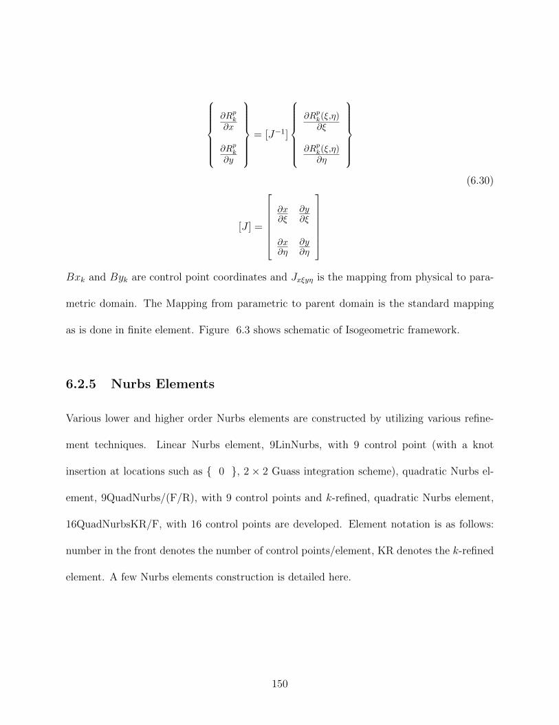
∂Rp
k
∂x
∂Rpk
∂y
= [J−1]
∂Rp
k(ξ,η)∂ξ
∂Rpk(ξ,η)∂η
[J ] =
∂x∂ξ
∂y∂ξ
∂x∂η
∂y∂η
(6.30)
Bxk and Byk are control point coordinates and Jxξyη is the mapping from physical to para-
metric domain. The Mapping from parametric to parent domain is the standard mapping
as is done in finite element. Figure 6.3 shows schematic of Isogeometric framework.
6.2.5 Nurbs Elements
Various lower and higher order Nurbs elements are constructed by utilizing various refine-
ment techniques. Linear Nurbs element, 9LinNurbs, with 9 control point (with a knot
insertion at locations such as 0 , 2 × 2 Guass integration scheme), quadratic Nurbs el-
ement, 9QuadNurbs/(F/R), with 9 control points and k-refined, quadratic Nurbs element,
16QuadNurbsKR/F, with 16 control points are developed. Element notation is as follows:
number in the front denotes the number of control points/element, KR denotes the k-refined
element. A few Nurbs elements construction is detailed here.
150

Figure 6.3: Mapping between physical and parent domain: a framework for Isogeometricfinite element analysis
Quadratic Nurbs Element (9QuadNurbs))
A tensor product of knot vector −1 − 1 − 1 1 1 1 in ξ and η direction results in a bi-
quadratic Nurbs element in the parent domain. ξi denote the ith knot value in the knot
vector. The element consists of 9 control points. The shape function in ξ direction can be
written as follows,
M21 (ξ) =
(ξ4 − ξξ4 − ξ2
)(ξ4 − ξξ4 − ξ3
)
151

M22 (ξ) =
(ξ − ξ2
ξ4 − ξ2
)(ξ4 − ξξ4 − ξ3
)+
(ξ5 − ξξ5 − ξ3
)(ξ − ξ3
ξ4 − ξ3
)ξ3 ≤ ξ < ξ4
M23 (ξ) =
(ξ − ξ3
ξ5 − ξ3
)(ξ − ξξ4 − ξ3
)(6.31)
k-refined Quadratic Nurbs element I(16QuadNurbsKR)
A tensor product of knot vector −1 − 1 − 1 0 1 1 1 in ξ and η direction results in a
quadratic Nurbs element, 16QuadNurbsKR1(F/R). The knot vector is divided into two inter-
vals and shape functions have unique value over each interval. ξi denote the ith knot value in
the knot vector. The shape functions in ξ direction over each interval are derived as follows,
M21 (ξ) =
(ξ4 − ξξ4 − ξ2
)(ξ4 − ξξ4 − ξ3
)
M22 (ξ) =
(ξ − ξ2
ξ4 − ξ2
)(ξ4− ξξ4 − ξ3
)+
(ξ5 − ξξ5 − ξ3
)(ξ − ξ3
ξ4 − ξ3
)ξ3 ≤ ξ < ξ4
M23 (ξ) =
(ξ − ξ3
ξ5 − ξ3
)(ξ − ξξ4 − ξ3
)(6.32)
M24 (ξ) = 0
M21 (ξ) = 0
M22 (ξ) =
(ξ5 − ξξ5 − ξ3
)(ξ5 − ξξ5 − ξ4
)
M23 (ξ) =
(ξ − ξ3
ξ5 − ξ3
)(ξ − ξξ4 − ξ3
)+
(ξ − ξ3
ξ5 − ξ3
)(ξ5 − ξξ5 − ξ3
)ξ4 ≤ ξ < ξ5
M24 (ξ) =
(ξ − ξ4
ξ6 − ξ4
)(ξ4 − ξξ5 − ξ4
)(6.33)
152
Similarly, the shape functions in η direction are obtained. The product rule yields 16 bi-
quadratic shape functions, R2k, requiring 4 × 4 Gauss points. In k-refinement process, the
order of the existing knot vector from base model is elevated first and then, a knot is inserted
instead of elevating the order after knot insertion. This results in q−1 continuous derivatives
instead of p−1 continuous derivatives, where p and q are the order of the knot vector before
and after the order elevation, respectively.
6.3 Numerical Testing
Laminated composite plates with various orientation and thickness ratios are studied for
validation purposes. Cross-ply and anti-symmetric angle ply composite laminated plate are
studied. Due to bi-axial symmetry, only a quadrant of the plate is modeled and fundamental
frequency and center deflection are plotted.
6.3.1 Simply supported, cross-ply (0/90/90/0), square plate
In this analysis, a simply-supported, square, laminated cross-ply plate is studied. Material
for each lamina is considered as homogeneous, elastic and orthotropic. Material properties
used are as follows: E1 = 25E2, G12 = G13 = 0.5E2, G13 = 0.2E2, ν12 = 0.25, and Ks = 5/6.
9QuadNurbs with 3×3 Gauss integration scheme and 9LinNurbs with 2×2 Gauss integration
schemes are considered. 2 × 2, 4 × 4 and 8 × 8 physical meshes are used in the analysis.
Effect of modulus in fiber direction on natural frequency is studied and compared with the
153

existing literature. Fundamental frequency for different elements is compared with exact
solution [116], [113], MLSDQ’s solution by Liew et al.[114] and RBF’s results [115] for the
coarsest mesh. Table 6.1 shows the fundamental frequency comparison for these elements.
E2/E1
Element Mesh 10 20 30 40
9quadNurbs 2×2 8.54 9.37 9.99 10.29
9quadNurbs 3×3 8.42 9.45 9.92 10.36
9LinNurbs 2×2 9.144 10.01 10.52 10.86
9LinNurbs 3×3 8.72 9.64 10.18 10.54
LinIsoNurbs 4×4 8.88 9.79 10.32 10.68
LinIsoNurbs 8×8 8.53 9.49 - -
LinIsoNurbs 16×16 8.376 - - -
MLSDQ 8.2924 9.5613 10.32 10.849
RBF 8.3101 9.5801 10.349 10.864
Exact 8.2982 9.5671 10.326 10.854
Table 6.1: Comparison of natural frequency of a simply supported, cross-ply (0/90/90/0)square plate for various E2/E1
154

6.3.2 Effect of span-to-thickness ratio on simply-supported, lami-
nated cross-ply (0/90/90/0), square plate
In this analysis, a simply-supported, square, cross-ply (0/90/90/0), laminated composite
plate with various span to thickness ratios, a/h = 5, 10, 20, 25, 50, 100, are analyzed. Material
for each lamina is considered as homogeneous, elastic and orthotropic. Material properties
used are as follows: E2/E1 = 40, G12 = G13 = 0.5E2, G23 = 0.2E2, ν12 = 0.25, and Ks = 5/6.
9QuadNurbs element with 3 × 3 Guass integration and 9LinNurbs element with 2 × 2
Guass integration scheme are used. Table 6.2 shows the fundamental frequency comparison
for these elements with 2 × 2 and 4 × 4 meshes. Comparisons are made with Reddy and
Phan [112], p−Ritz solution [114], RBF-pseudospectral method [115]. Table 6.2 shows the
comparison of fundamental frequency for various Nurbs elements. It is observed that lower
span to thickness ratio has considerable effect on natural frequency, however, the effect dies
down for higher a/h ratios.
6.3.3 Effect of Layup Sequence and Fiber Orientation
A simply supported, cross-ply (0/90/90/0), square laminate with a/h = 100, is studied for
free vibration analysis. The material properties used here are as follows : E1/E2 = 25;
G12/E2 = 0.50; G23/E2 = 0.20; G13 = G12; E2 = E3; ν12 = ν23 = ν13 = 0.25. This example
investigates the effect of layup sequence and fiber orientation for [θ/0/0/θ] and [0/θ/θ/0]
plies under simply-supported boundary conditions. Span to thickness ratio of a/h = 100
155

a/hElement Mesh 10 20 50 100
9quadNurbs 3×3 14.40 17.50 18.61 19.03
9LinNurbs 3×3 14.52 17.33 18.81 18.90
LinIsoNurbs 4×4 16.27 18.99 21.37 22.52
LinIsoNurbs 8×8 15.4865 18.20 19.84 20.37
LinIsoNurbs 16×16 15.177 17.92 19.39 19.74
HSDT 15.2689 17.6669 18.4624 18.7561
p-Ritz 15.1434 17.6583 18.6734 18.8359
RBF 15.1007 17.6338 18.6586 18.8223
Table 6.2: Comparison of natural frequency of a simply supported, cross-ply (0/90/90/0)
square plate for various a/h ratios with the literature (ω∗ = (ω ∗ a2/h)√ρ/E2)
156

and modulus ratio, E1/E2 = 10 is used in computation. Figures 6.4 and 6.5 shows the effect
of lay-up sequence and fiber orientation on natural frequency.
0 20 40 60 8015
16
17
18
19
20
θ
ω
9LinNurbs
9quadNurbs
Figure 6.4: Effect of fiber orientation and stacking sequence [0, θ, θ, 0] on natural frequencyof square laminated plate
0 20 40 60 8010
12
14
16
18
20
θ
ω
9LinNurbs
9quadNurbs
Figure 6.5: Effect of fiber orientation and stacking sequence [θ, 0, 0, θ] on natural frequencyof square laminated plate
157

6.3.4 Higher frequencies using higher order Nurbs elements
A simply supported (SS1), cross-ply laminate is studied here. The material properties
used here are as follows : E1/E2 = 40; G12/E2 = 0.60; G23/E2 = 0.5;G13 = G12; E2 = E3;
ν12 = ν23 = ν13 = 0.25. First five natural frequencies are computed in Table 6.3 for a/h = 10.
9QuadNurbs, 9LinNurbs and 16CubicNurbs and 16QuadNurbsKR elements are considered.
2× 2, 4× 4 and 8× 8 meshes are used for analysis. It is observed that 9LinNurbs element
computes lower frequencies than other elements considered.
Element Mesh ω∗1 ω∗2 ω∗3 ω∗4 ω∗5
9quadNurbs 4×4 14.48 44.07 53.65 68.17 86.15
9quadNurbs 8×8 14.48 43.88 53.55 67.97 84.94
9LinNurbs 4×4 13.295 40.05 50.03 63.49 82.23
9LinNurbs 8×8 13.185 40.26 49.33 67.97 84.94
16CubicNurbs 2×2 14.47 43.82 53.48 67.88 85.30
16quadNurbsKR 2×2 14.32 45.03 54.48 69.46 93.5
Table 6.3: Comparison of first five natural frequencies of a simply supported, cross-ply
(0/90/90/0) square plate for a/h = 10 for various Nurbs elements, (ω∗ = (ω ∗ a2/h)√ρ/E2)
6.3.5 Orthotropic Plate under step loading
A simply-supported (SS1), orthotropic plate is studied. The material properties used are
as follows:E1 = 525000; E2 = 21000 N/mm2; G12/E2 = 0.60; G23/E2 = 0.5; G13 = G12;
158
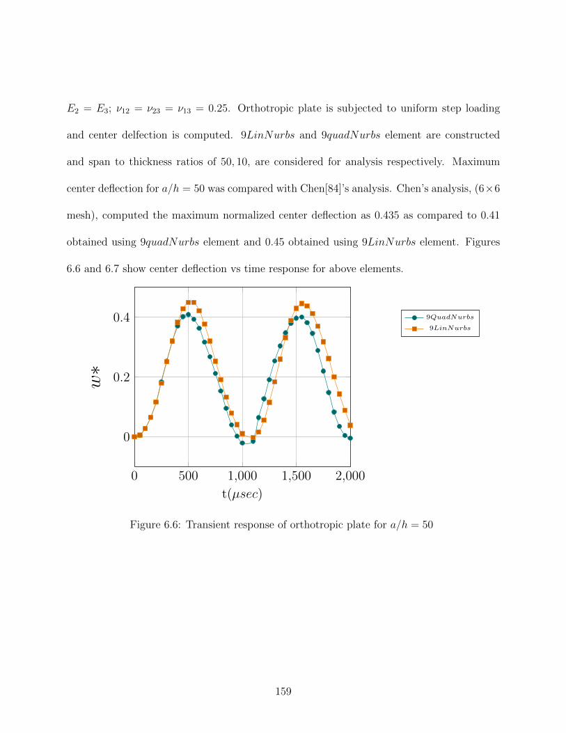
E2 = E3; ν12 = ν23 = ν13 = 0.25. Orthotropic plate is subjected to uniform step loading
and center delfection is computed. 9LinNurbs and 9quadNurbs element are constructed
and span to thickness ratios of 50, 10, are considered for analysis respectively. Maximum
center deflection for a/h = 50 was compared with Chen[84]’s analysis. Chen’s analysis, (6×6
mesh), computed the maximum normalized center deflection as 0.435 as compared to 0.41
obtained using 9quadNurbs element and 0.45 obtained using 9LinNurbs element. Figures
6.6 and 6.7 show center deflection vs time response for above elements.
0 500 1,000 1,500 2,000
0
0.2
0.4
t(µsec)
w∗
9QuadNurbs
9LinNurbs
Figure 6.6: Transient response of orthotropic plate for a/h = 50
159

0 100 200 300 400 500−0.1
0
0.1
0.2
0.3
t(µsec)
w∗
9LinNurbs
9quadNurbs
Figure 6.7: Transient response of orthotropic plate for a/h = 10
6.3.6 Four layer cross-ply and anti-symmetric angle-ply plates un-
der step loading
A simply-supported (SS1), cross-ply 0/90/90/0), composite plate is studied here. The
foloowing material properties were used here, E1 = 40E2; E2 = 21000 N/mm2; G12/E2 =
0.60; G23/E2 = 0.5; G13 = G12; E2 = E3; ν12 = ν23 = ν13 = 0.25. Transient analysis is
performed for span to thickness ratio, a/h = 50 and 9LinNurbs and 9quadNurbs are con-
sidered in this analysis. In Fig. 6.8, the center deflection vs time is plotted for the coarsest
mesh.
Anti-symmetric angle-ply layup introduces B16 and B26 coupling coefficients. Effect of these
coupling coeffcients are explored in this analysis. Transient analysis is performed for [45/−
160

0 500 1,000 1,500 2,000−1
0
1
2
t(µsec)
w∗
9quadNurbs
9LinNurbs
Figure 6.8: Transient response of laminated composite lay up (0/90/90/0) sequence fora/h = 50
45/45/ − 45] angle-ply layup for a/h = 50. 9LinNurbs and 9quadNurbs elements are
considered in this analysis. In Fig. 6.9, center deflection vs time response is plotted for
the coarsest mesh. It is observed that the center deflections are reduced in this case when
compared with the [0/90/90/0] lay-up. This is due to coupling coefficient contribution to
the stiffness matrix.
6.4 Conclusions
This chapter details the development of Nurbs Isogeometric finite element analysis code
for free vibration and linear dynamics analysis of composite plates. First-order, shear-
deformable laminate composite plate theory is utilized in deriving the governing equations
161

0 500 1,000 1,500 2,000−1
0
1
2
t(µsec)
w∗
9quadNurbs
9LinNurbs
Figure 6.9: Transient response of laminated composite lay up (45/− 45/45/− 45) sequencefor a/h = 50
using a variational formulation. Linear, quadratic, higher order and k-refined Nurbs elements
are constructed and numerical validation is performed for orthotropic, laminated composite
plates. Different ply to thickness ratios, modulus ratios and ply-angles are considered.
162
Chapter 7
Conclusion and Future Work
Inspite of the extensive use of finite element methods, the barriers between engineering
design and analysis still exist and the way to bridge gap is use the same model for analysis
as used in CAD. The idea, introduced by T.J.R. Hughes, to use the same CAD basis for
analysis purpose as used for geometry representation is known as Isogeometric analysis.
There are several CAD functions which can be used for Isogeometric analysis. Of most
widely used CAD basis in engineering design process are Nurbs (non-uniform rational B-
splines) as presented by Piegle and tiller[20], Farin[21], Cohen et al.[22] and Rogers[23]. The
CAD industry widely uses Nurbs to describe the smooth lines and surfaces. The curve or
surface generated using Nurbs depends on control points which are associated with unique
basis function. Thus, each vertex effects the shape of the curve over a range of parametric
values where the basis function is non-zero.
163
The CAD based functions such as bezier basis have been used for solving computational
mechanics problems. They offers advantage over the regular finite element due to their
piecewise form, smoothness and higher-order continuity. Besides that, these functions offer
computational efficiency, good accuracy and convergence characteristics. Nurbs basis possess
useful mathematical property of refinement through knot insertion and variational diminish-
ing property of convex hull i.e. curve does not oscillate about any straight line more than
its control polygon oscillates about the line.
Most finite element are still performed with low-order elements for which geometric errors are
largest. Isogeometric analysis entirely removes the finite element polynomial approximation
of geometry. Besides this, Nurbs basis are generated using recursion algorithm which tends
to improve the computational efficiency. Equation systems are more homogeneous as basis
have same shape on both ends. Nurbs basis are non negative and therefore, the mass matrix
is non-negative.
This research endevour develops Isogeometric approach for analysis of composite structures
and take advantage of higher order continuity, smoothness and variation dimishing properties
of Nurbs basis for interlaminar stress analysis of composite and sandwich structures. Nurbs
Isogeometric finite element analysis code is developed for analysis of composite plates in
(geometrically) nonlinear and linear range and for static and dynamic analysis. Besides
that, newer parent elements are also developed using refinement techonology of knot vector.
various Nurbs elements such as 9 control point linear (utilizing h-refinement), quadratic,
cubic and k-refined quadratic, cubic, quartic Nurbs element are constructed and validated
164

with numerical tesing. It is found that 9 control point linear Nurbs element removes shear
locking in linear and nonlinear ranges contrary to Nurbs quadratic and quadratic Lagrange
elements. Though, reduced integration removes shear locking, it accompanies with hourglass
instability or mesh distortion due to rank deficiency. 9 control point linear Nurbs element
and k-refined element technology removes this deficienicy without reducing the order of
integration, especially in nonlinear range.
Next, Nurbs post-processor for in-plane and interlaminar stress calculation in laminated com-
posite and sandwich plates is developed. Lagrange finite element suffers from higher order
stress gradient oscillations due to Gibbs phenomenon and require alternative stress recov-
ery procedures for accurate interlaminar stress calculations, especially interlaminar normal
stress. Researchers have developed higher order shear defromation theories and zig-zag theo-
ries for accurate prediction of interlaminar stresses. Here, direct Nurbs based post-processing
is performed which computes in-plane and interlaminar shear and normal stresses from higher
order gradients of Nurbs basis in a single step procedure. The stresses are found to be in
an excellent agreement with 3D elasticity solution and better than Lagrange finite element
and higher order shear deformation theory. Some of the elements perform exactly w.r.t 3D
elasticity solution which is due to higher order smoothness properties of Nurbs basis. In
beam analysis, B-spline basis developed using Cox-Deboor recursion algorithm
are found to be better than basis constructed using old form of B-splines in
terms of computational efficiency.
Next, stress analysis of laminated composite plate with open-hole using Nurbs Isogeometric
165
finite element analysis is developed. Geometry is modeled exactly in Isogeometric frame-
work and iso-parametric finite element representation is invoked for field variable defination.
Various refined Isogeometric meshes are generated for convergence study using h-refinement
process. h-refinement process is performed internally by inserting a single knot in the knot
vector and corresponding control net is obtained from the algorithm. Isotropic plate with
hole, (0/90)s and (−45/45)s composite laminates are studied under in-plane loading. Stress
concentration factor plays an important role in design consideration for composite structures
and free edge calculations are important. Here, stress concentration factor is computed along
the hole edge and compared with the literature. Convergence study is performed for vari-
ous Isogeometric meshes and stress convergence is obtained with increased mesh density. In
isotropic example, all the meshes converge to the same solution which matches the analytical
solution.
Next, Nurbs Isogeometric finite element code for free-vibration and linear dynamics analysis
of laminated composite plates is developed. First-order, shear-deformable laminate compos-
ite plate theory is utilized in deriving the governing equations using a variational formulation.
Linear, quadratic, higher order and k-refined Nurbs elements are constructed and numerical
validation is performed for orthotropic and laminated composite plates. Different ply to
thickness ratios, modulus ratios and ply-angles are considered. The results are found to be
in good agreement with the literature. Linear Nurbs Isogeometric analysis with one Gauss
integration point converges well, however, 9 control point linear Nurbs and quadratic Nurbs
elements perform better in terms of mesh refinement.
166

For future direction, the applications of the Nurbs based Isogeometric analysis are numerous.
Further direction can be to extend this code for analysis of plate with straight and curved
stiffners, buckling analysis, crack propagation analysis with XFEM, impact and crashwor-
thiness analysis, elastic-plastic analysis and for wave propagation in complex geometries like
pi-joints.
167

Bibliography
[1] Courant, R.,“Variational methods in solution of equilibrium and vibration,” of Amer-
ican Mathematical Society, Vol. 49, 1-43, 1943
[2] Zeinkeiwicz, O. C. and Cheung, Y. K.,The finite element method in structural and
continuum mechanics, McGraw-Hill
[3] Taig, I. C.,Structural analysis by matrix displacement method, Technical report, English
Electric Aviation
[4] Zeinkeiwicz, O. C., Taylor, R. L. and Too, J. M.,“Reduced integration technique in
general analysis of plates and shells,”International Journal of Numerical Methods in
Engineering, Vol. 3, 275-290, 1971
[5] Schoenberg, I. J.,“Contributions to the problems of approximation of equidistant data
by analytical functions,” Quart. Appl. Math., Vol. 4, 112-141, 1946
[6] DeBoor, C. R., “A Practical Guide to Splines ,” Springer-Verlag, 1978
168
[7] Gontier, C. and Vollmer, C.,“A large displacement analysis of a beam using a CAD
geometric definition,” Computers and Structures, Vol. 57, No. 6, 981-989, 1995
[8] Kagan, P., Fischer, A. and Yoseph, P. B.,“New B-spline finite element approach for ge-
ometrical design and mechanical analysis,”International Journal of Numerical methods
in Engineering, Vo. 41, 435-458, 1998
[9] Kagan, P., Fischer, A. and Yoseph, P. B.,“Mechanically based model: Adaptive re-
finement of B-spline finite element,”International Journal of Numerical methods in
Engineering, Vo. 57, 1145-1175, 2003
[10] Ganapathi, M., Patel, B. P., Saravanam, J., and Tousatier, M.,“Shear-flexible Curved
beam element for static analysis,”Finite Element in Analysis and Design, Vol. 32, pp.
181 - 202, 1999
[11] Chen, J. S., Han, W. and Meng, X.,“A reproducing kernel method with nodal interpo-
lation property,”International Journal of Numerical Methods in Engineering, Vol. 56,
pp. 935-960, 2003
[12] Atluri, S. N. and Shen, S. P., “The meshfree local Petrov-Galerkin (MLPG) method
,”Tech Science Press Encino, USA, 2002
[13] Atluri, S. N. and Zhu, T., “A meshfree local Petroc-Galerkin (MLPG) approach to
computational mechnics,”Computational Mechanics, Vol. 22, pp. 117-127, 1998
169
[14] Melenk, J. M. and Babuska, I.”The partition of unity finite element method: basic
theory and application ,”Computer Methods in Applied Mechanics and Engineering,
Vol. 139, pp. 289-314, 1996
[15] Babuska, I. and Melenk, J. M. “Partition of unity method,” International Journal of
Numerical Methods in Engineering, Vol. 40, pp. 727-758, 1997
[16] Rao, B. N. and Rahman, S.,“An element-free Galerkin method for probabilistic me-
chanics and reliability,”International Journal of Solids and Structures, Vol. 38, no.
50-51, pp. 9313-9330, 2001
[17] Belytschko, T., Organ, D. and Gerlach, C.,“Element-free Galerkin methods for dy-
namic fracture in concrete,”Computer Methods in Applied Mechanics and Engineering,
Vol. 48, no. 11, pp. 385-399, 2000
[18] Dolbow, J. and Belytschko, T.,“An introduction to programming the meshless element-
free Galerkin method,”Archives of Computational Methods in Engineering, Vol. 5, no.
3, pp. 207-241, 1998
[19] Liu, G. R., Yan, L. and Wang, J. G.,“A point integration method based on local
residual formulation using radial functions ,”Structural Engineering And Mechanics,
Vol. 14, no. 6, pp. 713-732, 2002
[20] Piegl, L., and Tiller, W.,The Nurbs book (Monograph in visual communication), 2nd
Edition, Springer-Verleg
170

[21] Farin, G.,Curves and Surfaces, A practical guide, 5th Edition, Morgan aufmann Pub-
lishers, 1950
[22] Cohen, E., Lyche, T., and Reisenfield, R.,“Discrete b-splines and subdivision tech-
niques in computer aided geometric design and computer graphics,” Computer graphics
and Image processing, Vol. 14, pp. 87-111, 1980
[23] Rogers, D. F.,“Introdution to Nurbs with historic prospective,”Academic Press, 1955
[24] Peters, J., and Reif, U.,“Subdivision surface,”Springer-Verlag
[25] Warren, J., and Weimer, H.,“Introdution to Nurbs with historic prospectiveSubdivision
methods for Geometric Design,”Morgan Kaufmann Publishers
[26] Gordon, W.,“Spline-blended interpolation through curve networks,”Journal of
Methamatics and Mechanics, Vol. 18, 931-952, 1969
[27] Gregory, J. A.,n-sided surface patches, N. Gregory, j. A. editor, Mathematics of Sur-
faces,Clarendon Press
[28] Loop, C. T., and DeRose, T. D.,“A multisided generalization of Bezier surfaces,” ACM
Transaction on Graphics, Vol. 8, 204-234, 1989
[29] Bajaj, C., Chen, J. and Xu, G.,“Modeling with cubic A-patches,”ACT Transactions
on Graphics, vol. 14, 103-133, 1995
171

[30] Hughes, T.J.R., Cottrell, J.A. and Bazilevs, Y.,“Isogeometric analysis: CAD, Finite
elements, Nurbs, exact geometry and mesh refinement,” Computer Methods in Applied
Mechanics and Engineering, Vol. 194 , 4135-4195, 2005
[31] Hughes, T.J.R, Reali, A. and Sangali, G.,“Duality and unified analysis of discrete
approximation in structural dynamics and wave propagation: comparison of p-method
finite elements with k-method Nurbs,”Comput. Meth. Appl. Mech. Engng., Vol. 197,
4104-4124, 2008
[32] Bazilevs, Y., Calo, V. M., Hughes, T.J.R. and Zhang, Y.,“Isogeometric fluid-structure
inreaction: theory, algorithm and computations, Comput. Mech., Vol. 38, 310-322,
2006
[33] Cottrel, J.A., Hughes, T.J.R. and Reali, A.,“Isogeometric analysis of structural vibra-
tion,”Computer Aided Geometric Design, Vol. 27, 644-655, 2010
[34] Vuong, A. V., Heinrich, Ch. and Simeon, B.,“ISOGAT: A 2D tutorial MATLAB code
for Isogeometric Analysis,”Comput. Meth. Appl. Mech. Eng., Vol. 196, 4160-4183, 2010
[35] Reissner, E.,“On the theory of bending of elastic plates,”Journal of Mathematical
Physics, 23, 184-191, 1944
[36] Reissner, E.,“Effect of transverse shear deformation on the bending of elastic
plates,”Journal of Applied Mechanics, 12, 69-77, 1945
172

[37] Mindlin, R.,“Influence of rotatory inertia and shear on flexural motions of isotropic,
elastic plates,” Journal of applied mechanics, 18, 31-38, 1951
[38] Whitney, J. and Pagano, N.,“Shear deformation in heterogeneous anisotropic plates,”
Journal of Applied Mechanics, Vol. 37, 1031-1036, 1970
[39] Urthaler, Y. and Reddy, J. N.,“A mixed finite element for the nonlinear bending anal-
ysis of laminated composite plates based on FSDT,” Mechanics of Advanced Materials
and Structures, Vol. 15, 335-354, 2008
[40] Putcha N. S. and Reddy, J. N.,“A refined mixed shear flexible finite element for the
nonlinear analysis of laminated plates,” Computer Structure, Vol. 22, 529-38, 1986
[41] Kant, T. and Kommineni, J. R.,“C0 finite element geometrically nonlinear analysis
of fibre reinforced composite and sandwich laminates based on a higher-order the-
ory,”Computers & Structures , Vol. 45, 511-520, 1992
[42] Polit, O. and Touratier, M.,“A multilayered/Sandwich triangular finite element applied
to linear and non-linear analyses,”Composite Structures, 121-128, 2002
[43] Reddy, J. N. and Robbins, DH. Jr,“Theories and computational models for composite
laminates,”Appl. Mech. Rev., Vol. 47, no. 6, 147 - 169, 1994
[44] Wang, C. M. and Reddy, J. N.“Shear deformable beams and plates: Relationship with
classical solutions,”Elsevier, Oxford, U. K., 2000
173
[45] Reddy, J. N. and Sandidge, D.,“Mixed finite element models for laminated composite
plates,”Journal of Engineering for Industry, Vol. 109, 39-45, 1986
[46] Zienkeiwicz, O. C., Taylor, R. L. and Too, J. M.,“Reduced integration technique in
general analysis of plates and shells,”International Journal for Numerical Methods in
Engineering, Vol. 3, pp. 275-290, 1971
[47] Hughes, T. J. R., Taylor, R. L. and Kanoknukuchai, W.,“A simple and efficient finite
element for plate bending,”International Journal for Numerical Methods in Engineer-
ing, Vol. 11, pp. 1529-1543, 1977
[48] MacNeal, R. H.,“Derivation of element stiffness matrices by assumed strain distribu-
tion,”Nuclear Engineering and Design, Vol. 70, pp. 3-12, 1982
[49] Bathe, K. J., and Dvorkin, E. N.,“A four-node plate bending element based on
Mindlin/Reissner plate theory and a mixed interpolation,”International Journal for
Numerical Methods in Engineering, Vol. 21, pp. 367-383, 1983
[50] Batoz, J. L. and Katili, I.,“On a simple triangular nine d.o.f element based on incom-
patible modes and discrete constraints,”International Journal for Numerical Methods
in Engineering, Vol. 35, pp. 1603-1632, 1992
[51] Zienkeiwicz, O. C., Zeng, L. F., Samuelsson, A., and Wiberg, N. E.,“Linked Interpola-
tion for Reissner-Mindlin Plate element: Part I- a simple quadrilateral.,”International
Journal for Numerical Methods in Engineering, Vol. 36, pp. 3043-3056, 1993
174

[52] Shi, Z. C., Ming, P. and Braess, D.,“Shear locking in a plane elasticity prolem and the
enhanced assumed strain method,”Siam J. Numer. Anal., Vol. 47, No. 9, 4479-4491,
2010
[53] Echer, R. and Bischoff, M.,“Numerical efficiency, locking and unlocking of Nurbs finite
elements,Comput. Meth. Appl. Mech. Eng., Vol. 199, 374-382, 2010
[54] Zhang, Y. X. and Kim, K. S.,“Geometrically nonlinear analysis of laminated com-
posite plates by two new displacement-based quadrilateral plate elements,”Composite
Structures, Vol. 72, 301 - 310, 2006
[55] Minghini, F., Tullini, N., and Laudiero, F.,“Locking-free finite element for shear de-
formable orthotropic thin-walled beams,”International Journal for Numerical Methods
in Engineering, Vol. 72, 808-834, 2007
[56] Nguyen-Xuan, H., Rabczuk, T., Bordas, S., and Debongnie, J. F.,“A Smoothed Finite
Element for Plate Analysis,”Computational Methods for Applied Mechanics Engineer-
ing, Vol. 197, pp. 1184-1203, 2008
[57] Cai, Y. C., Tian, L. G., and Atluri, S. N.,“A Simple Locking Free Discrete Shear
Triangular Plate Element,”CMES, Vol. 77, no. 4, pp. 221-238, 2011
[58] Bathe, K. J.“The Finite Element Methods,”Prentice-Hall, Englewood Cliffs, NNJ/MA,
1987
175

[59] Bathe, K. J.,A Finite Element Procedures, Prentice-Hall/MIT ,Englewood Cliffs,
NNJ/MA, 1996
[60] Zienkiewicz, O. C., Taylor, R. L.,“The Finite Element Methods, fifth ed.,”Oxford,
Butterworht-Heinemann, 2000
[61] Flanagan, T. P., and Belytschko, T.,“A uniform strain hexahedron and quadrilateral
with orthogonal hourglass control,” Int. j. Numer. Methods Engng., Vol. 17, 679-706,
1981
[62] Tessler, A. and Hughes, T.J.R.,“An improved treatment of transverse shear in the
Mindlin-type four node quadrilateral element,” Comput. Methods Appl. Mech. Engng.,
Vol. 39, 311-335, 1983
[63] Phan, ND. and Reddy, J. N.,“Analysis of laminated composite plate using a higher
order shear deformation theory,” International Journal for Numerical Methods in En-
gineering, Vol. 21(12), 2201-19, 1985
[64] Ren, J. G. and Hinton, E.,“The finite element analysis of homogeneous and laminated
composite plates using a simple higher order theory. Communications in Applied Nu-
merical methods, Vol. 2(2), 217-28, 1986
[65] Codina, R.,“On stabilized finite element methods for linear systems of convection-
diffusion-reaction equations,” Comput. Methods Appli. Mech. Engng., Vol. 188, 61-82,
2000
176

[66] Lyly, M. and Stenberg, R.,“On the connection between some linear triangular
Riessener-Mindlin plate bending elements,” Numer. Math., Vol. 85, 77-107, 2000
[67] Tessler, A.,“Accurate interlaminar stress recovery from finite element analysis,” NASA
Technical Memorandum, NASA-TM-109149, Sept. 1994
[68] Reddy, J. N.,“A simple higher order theory for laminated composite plates,” Journal
of Applied Mechanics, Vol. 51, pp. 745-752, Dec. 1984
[69] Byun, C., and Kapania, R. K.,“Prediction of interlaminar stresses in laminated plates
using the global orthogonal interpolation polynomials,” AIAA Journal, Vol. 30, No.
11, Nov. 1992
[70] Lee, K., and Lee, S.,“A post-processing approach to determine transverse stresses in
geometrically nonlinear composite and sandwich structures“, Journal of Composite
Materials, Vol. 37, pp. 2207 - 2224, 1996
[71] Park, J. W., and Kim, Y. H.,“Displacement, stresses and their sensitivity coefficients
in composite panels,” Journal of Composite Materials, Vol. 33, No. 13, pp. 1222 -1243,
1999
[72] Park, B. P., Park, J. W., and Kim, Y. H.,“Stress recovery in laminated composite
and sandwich panels undergoing finite rotation,” Composite Structures, vol. 59, pp.
227-235, 2003
177
[73] Noor, A. K., Kim, Y. H., and Peters, J. M.,“Transverse shear stresses and their sen-
sitivity coefficients in multi-layered composite panels,” AIAA Journal, Vol. 32, No. 6,
pp. 1259-1269, 1994
[74] Matsunaga, H.,“Interlaminar stress analysis of laminated composite beams to global
higher-order deformation theories,”Composite Structures, Vol. 55, pp. 105-114, 2002
[75] Makeev, A., and Armanios, E. A.,“An iterative method for solving elasticity problems
for composite laminates,”ASME Journal of Applied Mechanics, Vol. 67, No. 1, March
2000
[76] Rolfes, R. and Rohwer, K.,“Improved transverse shear stresses in composite finite
elements based on the first order shear deformation theory,” International Journal for
Numerical Methods in Engineering, Vol. 40, pp. 51 - 60, 1997
[77] Kant, T., and Manjunatha, B. S.,“On accurate estimation of transverse stresses in
multilayer composites,” Computers and Structures, Vol. 50, No. 3, pp. 3451 - 365,
1994
[78] Kant, T., Gupta, A. B., Pendhari, S. S., and Desai, Y. M.,“Elasticity solution of cross-
ply composite and sandwich laminate,” Computers and Structures, Vol. 83, No. 1, pp.
13-24, March, 2008
[79] Nosier, A., and Baharami, A.,“Interlaminar stresses in antisymmetric angle - ply lam-
inates,” Composite Structures, Vol. 78, pp. 18 - 33, 2007
178
[80] S. S. Vel, and Batra, R. C.,“Analytical solutions for rectangular thick laminated plates
subjected to arbitrary boundary conditions,” AIAA Journal, Vol. 37, pp. 1464-1473,
1999
[81] Barlow, J.,“Optimal stress locations in finite element models,” Int. J. Numer. Methods,
Vol. 10(2), pp. 243-251, 1976
[82] Oden, J. T., and Brachli, H. J.,“On the calculation of consistent stress distribution in
finite element approximation,”Int. J. Numer. Methods, Vol. 10(2), pp. 243-251, 1971
[83] Hinton, J. S., and Cambell, E.,“Local and global smoothing of discontinuous finite
element functions using a least square method,”Int. J. Numer. Methods, Vol. 8(3), pp.
461-480, 1974
[84] Chen, D. J., Shah, D. K., and Chan, W. S.,“Interfacial stress estimation using least-
square extrapolation and local stress smoothing in a laminated composites,”Computer
Structures, Vol. 58, pp. 765-774, 1996
[85] Zienkiewicz, O.C. and Zhu, J. Z.,“The super convergent patch recovery and a posteriori
erro estimates. Part I: the recovery technique,”Int. J. Numer. Methods Eng, Vol. 33(7),
pp. 1331-64, 1992
[86] Yuan, J., Saleeb, A., and Gendy,, A.,“Projection stress: layerwise- equivalent formu-
lation for accurate prediction of transverse stresses in laminated plate and shells,”Int.
J. Computat. Eng. Sci, Vol. 1(1), pp. 91-138, 1982
179

[87] Prathap, G., and Naganarayana, B. P.,“Consistent thermal stress evaluation in finite
elements,”Comput. Struc, Vol. 54(3), pp. 415-46, 1995
[88] Tang, S.,“Interlaminar stresses around circular cutouts in composite plates under ten-
sion,”AIAA Journal, Vol. 15(11), pp. 1631-37, 1976
[89] Tang, S.,“A variational approach to edge stresses of circular cutouts in compos-
ites,”20th AIAA/ASME/ASCE/AHS, SDM Conference, St. Louis, MO, AIAA Paper
79-0802, pp. 326-32, 1979
[90] RamKumar, R. L., Saether, E. S., and Cheng, D.,“Design guide for bolted joints in
composite structures,”AFWAL-TR-86-3035, 1986
[91] Soni, S. R.,“Stress and strength analysis of bolted joints in composite lami-
nates,”Composite Structures, Vol. 03, pp. 50-62, 1981
[92] Nishioka, T., and Atluri, S. N.,“Stress analysis of holes in angle-ply laminates:
an efficient assumed stress special hole element approach and a simple estimation
method,”Computer Structures, Vol. 15(2), pp. 135-147, 1982
[93] Iarve, E. V., “Spline variational three dimensional stress analysis of laminated com-
posite plates with open holes,”International Journal of Solid Structures, Vol. 33(14),
pp. 2095-2118, 1996
180

[94] Raju, I. S., and Crews, Jr.,“Three dimensional analysis of [0/90]s and [90/0]s laminates
with a central circular hole,”Composite Technology Review , Vol. 4(4), pp. 116-124,
1982
[95] Folias, E. S.,“Boundary layer effects of interlaminar stress analysis at free edges of
composite laminate,”Computers Structure , Vol. 29, pp. 171-186, 1992
[96] Bar Yoseph, P. and Avrashi, G.“Interlaminar stress analysis of laminated plates con-
taining a curvilinear hole,”Computers Structure , Vol. 21, pp. 917-932, 1985
[97] Pan, E., Yang, B., Cai, G. and Yuan, F. G.“Stress analysis around holes in compos-
ite laminates using boundary element method,”Engineering Analysis with Boundary
Elements , Vol. 25, pp. 31-40, 2001
[98] Rybivki, E. F., and Hopper, A. T.“Analytical investigation of stress concentrations due
to holes in fiber reinforced plastci laminated plates: three-dimensional models,”AFML-
TR-73-100 , Battlelle, Columbus Labs, 1973
[99] Bert, C. W.,“Research on dynamics of composite sandwich plates,”Shock and Vibration
Digets, Vol. 14, pp. 17-34, 1982
[100] Mohammad, S. Q.,“Recent research advances in the dynamic behavior of shell: 1989-
2000, Part 1: Laminated composite shells,”ASME Applied Mechanics Reviews, Vol.
55(4), pp. 325-350, 2002
181

[101] Song, S., and Waas, A.,“Effects of shear deformation on buckling and free vibration of
laminated composite beams,”Composite Structures, Vol. 37(1), pp. 33-43, 1997
[102] Lim, S. p. Chen, X. L. and Liu, G. R.,“An element free Galerkin method for free
vibration analysis of composite laminates,”Composite Structures, Vol. 47, pp. 101-127,
2000
[103] Liew, K. M., Huang, Y. Q., and Reddy, J. N.,“Vibration analysis of symmetrically
laminated plates based on FSDT using moving least square differential quadrature
method,”Computer Methods in Applied Mechanics and Engineering, Vol. 192, pp. 2203-
2222, 2003
[104] Ferreira, A. J. M., and Roque, C. M. C.,“Free vibration analysis of symmetric lam-
inated composite plates by FSDT and radial basis functions,”Computer Methods in
Applied Mechanics and Engineering, Vol. 194, pp. 4265-4278, 2005
[105] Liu, G. R., Dai, K. Y. and Nguyen, T. T.,“A smoothed finite element method for
mechanics problems,”Computational Mechanics, Vol. 39(6), pp. 859-877, 2007
[106] Liu, G. R., Nguyen, T. T., Dai, K. Y. and Lam, K. Y.,“Theoretical aspects of smoothed
finite element method (SFEM),”International Journal for Nimerical Methods in Engi-
neering, Vol. 71(8), pp. 902-930, 2006
[107] Kapania, R. K. and Raciti, S.,“Recent advances in Analysis of Laminated Beams and
Plates, Part II : Vibrations and wave propagation’,” AIAA Journal, Vol. 27, No. 7,
July, 1989
182
[108] Kapania, R., K. and Raciti, S.,“Recent Advances in Analysis of Laminated Beams and
Plates, Part I : Shear effects and Buckling’,” AIAA Journal, Vol. 27, No. 7, July, 1989
[109] Reddy, J. N.,“Mechanics of Laminated composite plates and shells,” CRC Press, 2000
[110] Levy, S.,“Square plate with clamped edges under normal pressure producing large
deflection,”Tech. Report, National Advisory Committee for Aeronautics, 1942
[111] Argyris, J., and Tanek, L.,“Linear and geometrically nonlinear bending of isotropic and
multilayered composite plates by natural mode method,”Comput. Meth. Appl. Mech
Eng, Vol. 113, 207 - 51, 1994
[112] Reddy, J. N. and Phan, P. H.,“Stability and vibration of isotropic, orthotropic and
laminated plates according to a higher order shear deformation theory,”Journal of
Sound and Vibration, Vol. 89, pp. 157-170, 1985
[113] Ferreira, A. J. M. and Fasshauer, G. E.,“Analysis of natural frequencies of composite
plates by RBF-pseudospectral method,”Composite Structures, Vol. 79(2), pp. 202-210,
2007
[114] Reddy, J. N.,“An introduction to nonlinear finite element analysis,”Oxford University
Press
[115] Khdeir, A. A. and Librescu, L.,“Analysis of symmetric cross-ply elastic plates using a
higher-order theory. Part II: buckling and free vibration,”Composite Structures, Vol.
9, pp. 259-277, 1988
183

[116] Liew, K. M.,“Solving the vibration of thick symmetrric laminates by Reissner/Mindlin
plate theory and p-Ritz method,”Journal of Sound and Vibration, Vol. 198, pp. 343-
360, 1996
-
184