Is change worth it? The effects of adopting modern

African Journal of Agricultural and Resource Economics Volume 16 Number 3 pages 216-236

Is change worth it? The effects of adopting modern agricultural

inputs on household welfare in Rwanda

Aimable Nsabimana

Department of Economics, University of Rwanda, Kigali. E-mail: [email protected]

Abstract

This study investigates the driving factors that influence farmers’ decisions to adopt modern

agricultural inputs (MAI) and how this affects farm household welfare in rural Rwanda. To account

for heterogeneity in the MAI adoption decision and unobservable farm and household attributes, we

estimate an endogenous switching regression (ESR) model. The findings reveal that size of land

endowment, access to farm credit and awareness of farm advisory services are the main driving

forces behind MAI adoption. The analysis further shows that MAI adoption increases household farm

income, farm yield and equivalised consumption per capita. This implies that adopting MAI is the

most consistent and potentially best pathway to reduce poverty among rural farmers. The study hence

suggests that policymakers should align the effective dissemination of MAI information and farm

advisory services, strengthen farm credit systems and improve market access – most crucially at

affordable prices – among small-farmers throughout Rwanda.

Key words: modern agricultural inputs; welfare effect; endogenous switching regression; Rwanda

1. Introduction

Sub-Saharan Africa (SSA) continues to face endless food shortages. The region is characterised by

a high incidence of malnutrition and food insecurity. Although the continent contains around 60% of

the world’s uncultivated arable land, SSA remains a net importer of food. A number of driving factors

that induce food shortages include unpredictable weather, which often results in production

uncertainty and unforeseen hardships for farm households, and the limited uptake of modern farm

inputs, which leads to lower farm yields and complete harvest failure, resulting in constant, severe

food shortages and welfare losses. Hence, these factors cause the farm yield across most of the SSA

countries to be inadequate for achieving food security (Sánchez 2010). To improve farm productivity

for smallholder farmers in particular, households need to adopt modern agricultural inputs (MAI).

These include the use of improved seeds, fertiliser and pesticides, and better ways of planting and

weeding.

However, despite its potential benefits, the adoption of MAI has been inconsistent and slow in some

farming systems, especially in SSA countries. This delay, and the erratic use of new and more

appropriate seed varieties, fertilisers and pesticides in many parts of SSA, have led to production

failures and ultimately have left the region with persistent hunger, food insecurity for families and a

high prevalence of poverty (Barrett 2013). Furthermore, the extant literature has also associated the

delay and low input uptakes with farm credit constraints, barriers to adequate information, poor

institutional arrangements and environmental factors, all of which lead to excessive production costs

(Barrett et al. 2004; Abdulai & Huffman 2014).

In addition, many driving forces have been attributed to the low farm yield in the agricultural sector

in the region. These include negative effects resulting from climate change (Jayne et al. 2018), the

AfJARE Vol 16 No 3 September 2021 Nsabimana

217

limited adoption rate of modern farm inputs (Abdulai 2016), and poor and unsustainable farming

practices (Graboswki et al. 2016), among others. It further has been also noticed that adopting modern

farm inputs allows farmers to deal with very serious issues related to climate change (Chavas & Shi

2015) and the rain-fed nature of farm production (Dzanku et al. 2015; Tesfaye et al. 2019). From

these binding constraints, the use of modern farm inputs in the agricultural sector in SSA is a sine qua

non condition for improving the agricultural sector and wellbeing of a significant number of

households that depend crucially on the farm sector. It is also important to mention that the use of

MAI could improve the fertility of the soil and the yield of crops (Khonje et al. 2018; Tesfaye et al.

2019).

The main objective of this study therefore was to examine the effects of MAI adoption on the welfare

of farmers. The MAI evaluated in this study are improved seed varieties, inorganic fertilisers,

pesticides and water conservation practices. The study was carried out against the backdrop of low

farm yield in Rwanda due to reliance on rain-fed agriculture, high levels of poverty and declining soil

fertility associated with nutrient depletion and soil erosion (Morris et al. 2007).

The purpose of this research, firstly, was to complement the extant literature on understanding

farmers’ decisions to adopt MAI in Africa, focusing on Rwanda. The fact is that Rwanda is a

subsistence farming country, where more than 75% of households depend daily on farming (World

Bank 2011). The research findings on farm technology therefore would be useful for policy makers

in helping them to design adequate and sustainable agriculture that can provide an optimal food

supply to meet the needs of the market. Second, we focus on the farm yield, income and farmers’

consumption expenditure (including net household welfare), as motivated by their implications for

achieving food security. Moreover, the use of farm yield and farm income seems particularly

appropriate in the Rwandan context. The country has initiated various farm policies, including land

use policy and a land consolidation programme (CIP). The latter was introduced in 2008 with the

overall goal of ensuring sustainable land management and improving farm yields (Ministry of

Agriculture 2011a). Under this programme, the country aimed to enhance the farm productivity of

priority crops, namely beans, maize, Irish potatoes, cassava, wheat and soybean, and the provision of

farm inputs, such as improved seeds and chemical fertilisers. As is the case in many other African

countries, Rwanda has faced intensive demographic pressure over the last decades, and this has also

created massive pressure on land use (both extensive housing and farming on fragmented land).

Hence, examining the effect of MAI on the welfare of smallholder farmers in Rwanda is crucial to

understand technology adoption processes and will offer scientific lessons for many other African

countries facing the challenges of high population pressure, high fertility rates, urbanisation,

unbalanced diets, food insecurity, malnutrition and low uptake of inputs.

To conduct the study, we applied an endogenous switching regression (ESR) model based on farm

household-level data collected from the national living standard household survey of Rwanda. The

former is very robust and an effective econometric technique that accounts for selectivity bias to

identify the welfare implications of MAI for smallholder farmers. By using the ESR technique, I was

able to derive unbiased treatment effects of MAI adoption on farm household welfare, and also

considered that MAI adoption may systematically change the production elasticities of farm inputs

and other relevant factors (Kabunga et al. 2011).

The findings from this study provide evidence of direct and indirect effects of MAI adoption on farm

household wellbeing. This will be of significant relevance for better understanding the yield effects

of MAI in Rwanda and other countries. An assessment of the empirical evidence is also important for

policy-making purposes (Winters et al. 2011), for example when designing and implementing

effective support measures.


218

The rest of the paper is organised as follows: Section 2 illustrates what is known about MAI adoption

in Rwanda. Section 3 explains the data sources and descriptive statistics, while section 4 presents the

theoretical model and the employed estimation techniques. Section 5 presents and discusses the

study’s findings. The last section concludes and provides policy implications.

2. What is known about MAI adoption in Rwanda?

Agricultural policies in Rwanda are implemented under crop intensification programmes (CIP), with

the aim of sustainably improving agricultural productivity through procuring improved seeds,

fertilisers and pesticides for farmers to increase crop production potential (Cantore 2011). In line with

boosting MAI adoption among small-scale farmers, different national policies have been proposed,

e.g. establishing the National Seed Service in 2001, the Seeds Law in 2003, the Seeds Commodity

Chain Project in 2005 and the National Seed Policy in 2007 (Kelly et al. 2001; African Seed Traders

Association [AFSTA] 2010). Moreover, CIP promotes new farming techniques among farmers with

the aim of assisting them to access new, improved agricultural inputs and to increase agricultural

productivity in food crops with high yield potential (beans, potatoes and maize, among others), thus

ensuring food security and self-sufficiency (Ministry of Agriculture 2011b). Under the CIP, farmers,

especially those involved in cooperatives and land consolidation programmes, are supported to access

farm inputs in the form of cooperative vouchers and, to a limited extent, farm credits under the so-

called Business Development Fund (BDF) projects.1 Besides, agriculture is still the main sector of

economic growth in Rwanda; it employs approximately 80% of the total labour force and generates

more than 43% of the country’s export revenues. Despite significant interventions by government

and stakeholders, the number of farmers using MAI is still insignificant. For instance, the National

Institute of Statistics of Rwanda ([NISR] 2015) showed that only 11.6% of smallholder farmers used

improved seeds, while the use of inorganic and organic fertilisers was only 14.6% and 43.1%

respectively during cropping season B in 2015.2 The adoption of MAI is also unimpressive in large-

scale farming, where improved seeds were used by 40% of farmers, while organic and inorganic

fertilisers were used by 42.3% and 51.5% of the farmers respectively during season B. In this study,

a farmer was considered to have adopted MAI if he/she had used at least two or more of the selected

inputs over the 12 months prior to the survey, otherwise the farmer was regarded as a non-adopter.

3. Data source and descriptive analysis

The data used in this study was extracted from the Third Integrated Household Living Conditions

Survey of Rwanda (EICV3), conducted in 2010/2011 by the NISR, together with the World Bank and

the EU, which provided financial and technical support. The survey encompassed the entire country

and included all four provinces, with the South, East and West provinces each accounting for 31%,

28% and 21% of the sampled farm households respectively, while the Northern province accounted

for 19% of the sample.3 The sample was restricted to households with farm activities to ensure that

all households in the adopt and non-adopt groups had engaged in farm economic activities in the 12

months before the survey was conducted (see Table 1). EICV3 provides information on household

farm income and farm yield level.

1 Initiated in 2009, BDF is a government project aimed at enhancing financing for small and medium-sized businesses,

especially those with innovative projects and employment potential. Since its implementation, BDF has made significant

contributions, especially to small-scale businesses – including farmers, who get access to farm credits. 2 Rwanda has three main agricultural seasons (A, B and C). Season A runs from September to January and season B from

February to May; both A and B are rainy seasons. The quantity of rainfall that occurs has a direct effect on crop production

and hence on food market prices. Season C runs from June to September and is a dry season, during which large crop

harvests take place, especially of grain crops such as rice, maize and wheat, and starch crops such as cassava and tuber

potatoes, among others. 3 To minimise the bias, city dwellers were removed from the study, as we were interested in farming, which is undertaken

mainly by rural inhabitants.


219

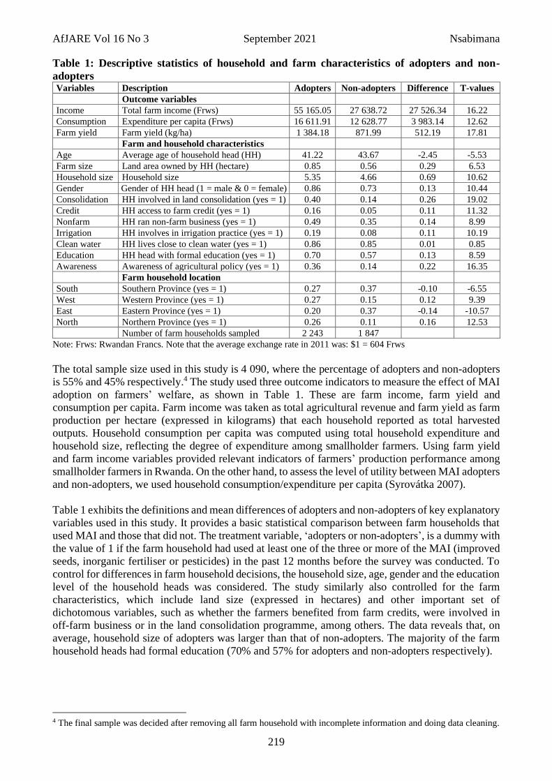
Table 1: Descriptive statistics of household and farm characteristics of adopters and non-

adopters Variables Description Adopters Non-adopters Difference T-values

Outcome variables

Income Total farm income (Frws) 55 165.05 27 638.72 27 526.34 16.22

Consumption Expenditure per capita (Frws) 16 611.91 12 628.77 3 983.14 12.62

Farm yield Farm yield (kg/ha) 1 384.18 871.99 512.19 17.81

Farm and household characteristics

Age Average age of household head (HH) 41.22 43.67 -2.45 -5.53

Farm size Land area owned by HH (hectare) 0.85 0.56 0.29 6.53

Household size Household size 5.35 4.66 0.69 10.62

Gender Gender of HH head (1 = male & 0 = female) 0.86 0.73 0.13 10.44

Consolidation HH involved in land consolidation (yes = 1) 0.40 0.14 0.26 19.02

Credit HH access to farm credit (yes = 1) 0.16 0.05 0.11 11.32

Nonfarm HH ran non-farm business (yes = 1) 0.49 0.35 0.14 8.99

Irrigation HH involves in irrigation practice (yes = 1) 0.19 0.08 0.11 10.19

Clean water HH lives close to clean water (yes = 1) 0.86 0.85 0.01 0.85

Education HH head with formal education (yes = 1) 0.70 0.57 0.13 8.59

Awareness Awareness of agricultural policy (yes = 1) 0.36 0.14 0.22 16.35

Farm household location

South Southern Province (yes = 1) 0.27 0.37 -0.10 -6.55

West Western Province (yes = 1) 0.27 0.15 0.12 9.39

East Eastern Province (yes = 1) 0.20 0.37 -0.14 -10.57

North Northern Province (yes = 1) 0.26 0.11 0.16 12.53

Number of farm households sampled 2 243 1 847

Note: Frws: Rwandan Francs. Note that the average exchange rate in 2011 was: $1 = 604 Frws

The total sample size used in this study is 4 090, where the percentage of adopters and non-adopters

is 55% and 45% respectively.4 The study used three outcome indicators to measure the effect of MAI

adoption on farmers’ welfare, as shown in Table 1. These are farm income, farm yield and

consumption per capita. Farm income was taken as total agricultural revenue and farm yield as farm

production per hectare (expressed in kilograms) that each household reported as total harvested

outputs. Household consumption per capita was computed using total household expenditure and

household size, reflecting the degree of expenditure among smallholder farmers. Using farm yield

and farm income variables provided relevant indicators of farmers’ production performance among

smallholder farmers in Rwanda. On the other hand, to assess the level of utility between MAI adopters

and non-adopters, we used household consumption/expenditure per capita (Syrovátka 2007).

Table 1 exhibits the definitions and mean differences of adopters and non-adopters of key explanatory

variables used in this study. It provides a basic statistical comparison between farm households that

used MAI and those that did not. The treatment variable, ‘adopters or non-adopters’, is a dummy with

the value of 1 if the farm household had used at least one of the three or more of the MAI (improved

seeds, inorganic fertiliser or pesticides) in the past 12 months before the survey was conducted. To

control for differences in farm household decisions, the household size, age, gender and the education

level of the household heads was considered. The study similarly also controlled for the farm

characteristics, which include land size (expressed in hectares) and other important set of

dichotomous variables, such as whether the farmers benefited from farm credits, were involved in

off-farm business or in the land consolidation programme, among others. The data reveals that, on

average, household size of adopters was larger than that of non-adopters. The majority of the farm

household heads had formal education (70% and 57% for adopters and non-adopters respectively).

4 The final sample was decided after removing all farm household with incomplete information and doing data cleaning.


220

4. Methodology and estimation techniques

4.1 Adoption decision and selection bias

As in other SSA countries, rural livelihoods in Rwanda are characterised by limited employment

opportunities besides for farming activities. The limited access to input markets and merit goods, and

poor infrastructure, among others, lead to high level of market failure. These market imperfections

translate into poverty, high transaction costs and underdevelopment for both the off-farm and farm

sectors. In this situation, it is difficult for rural households to access credit to purchase farm inputs to

increase agricultural productivity. Therefore, because of such conditions, the consumption and

production of rural households are not independent of one another. This means that farm household

resources are simultaneously allocated to off-farm labour supply and to on-farm activities like MAI

adoption (De Janvry et al. 1991; Asfaw et al. 2012). In such a scenario, it is possible that the adoption

of MAI by farmers would have positive effects on their welfare through increased crop yield, farm

income and employment opportunities, both inside and outside farming. In this respect, MAI adoption

could be expected to generate a high level of consumption, food market stability, higher farm income

and reduced poverty levels among households. The adoption of MAI would also free up household

resources for alternative uses and broadly improve farm household welfare. To model this type of

farm household behaviour, we assumed that farmers’ choice decision to adopt can be represented by

the random utility framework (Kabunga et al. 2012). For risk-neutral farmers, the decision to adopt

is based on comparing the expected utility of wealth from adoption, 𝑈𝐴(𝜔), against wealth of not

adopting, 𝑈𝑁(𝜔), with (𝜔) representing the amount of wealth. Therefore, farmers will adopt only if

𝑈𝐴(𝜔) > 𝑈𝑁(𝜔). The difference between utilities from adoption and non-adoption can be

expressed as:

( )* ( ) A N

hL U U = − , (1)

with *

hL being a latent variable to denote the difference between utility from MAI adoption, UA(ω),

and the utility from non-adoption, UN(ω). However, utilities are unobservable and can be expressed

as a function of observable elements in the following model:

* ,h h hL = +X η with *1 if 0

0 otherwise,

h

h

LL

=

, (1)

such that farm household h will choose to adopt (Lh = 1) by applying some of MAI in his/her farm

production strategies with the aim of improving farm yield, if *

hL > 0, and 0 otherwise. The vector

hX represents farm and household characteristics that affect the expected benefits of MAI adoption.

The characteristics are considered as driving factors of farmers’ adoption decision; 𝛈 is a coefficient

vector to be estimated, and 𝜇ℎ is the error term. To measure the effect of adoption, a baseline model

is presented, as follows:

h h h hL = + +Y Z , (3)

where 𝒀𝒉 is vector of outcome variables (farm income, productivity and expenditure per capita, all

three expressed in logarithms); 𝐿ℎ is an indicator variable for MAI adoption, as defined earlier; 𝒁𝒉 is

a vector of farm and household characteristics (such as education, age, land size); 𝛾 and 𝛿 are the

vectors of parameters to be estimated; and, finally, 휀ℎ is the stochastic disturbance term. From

equation (3), the effect of MAI adoption is measured by parameter 𝛿. However, for 𝛿 to be consistent


221

in measuring the effect of MAI adoption on farmers, it must be assigned randomly within the adopter

and non-adopter groups (Faltermeier & Abdulai 2009; Kassie et al. 2011). Unfortunately, the

adoption decision is not random in the case of the current dataset, thus inducing self-selection bias.

The farmers’ adoption decision depends on a set of observable and unobservable farm and household

characteristics that may be correlated with outcome values. These characteristics include farmers’

management skills, farm size, land fertility, farm landscape, government policies, farmers’ awareness

of MAI adoption, farm neighbourhood and many others. This leads to violation of the orthogonality

assumption, i.e. 𝐸(𝐿ℎ, 휀ℎ) ≠ 0. Different approaches have been suggested to deal with self-selection

bias. Heckman (1979) proposed a two-stage method dealing with a self-selection problem when the

correlation between two error terms is greater than zero. However, the approach accounts for selection

bias in unobservables only by treating the selectivity as an omitted variable problem (Abdulai &

Huffman 2014). The second approach is the propensity score matching (PSM) method proposed by

Rosenbaum and Rubin (1983), which has been used extensively with impact evaluation analysis in

various studies (Jalan & Ravallion 2003; Faltermeier & Abdulai 2009; Kassie et al. 2011). However, concerns have been expressed in the literature that PSM can only account for observable factors (Ma

& Abdulai 2016). This is a major drawback with the approach, as most of the treatments have

unobservable factors that also need to be considered to identify individual treatment effects on

outcomes.

In the current study, we examined the driving forces of MAI adoption and the effects of adoption

based on the endogenous switching regression (ESR) model. Using the ESR model, we

simultaneously estimated the factors and effect of MAI adoption by also accounting for both

observable and unobservable factors. The model further allowed us to account for selectivity bias in

deriving the effect of adoption on the outcomes. Developed by Lee (1982), the ESR method is a

generalisation of Heckman’s selection correction approach. The method accounts for unobservable

heterogeneity by considering the selectivity as omitted variable bias (Heckman 1979). Unlike the

Heckman model, our outcome variables in this study includes farm income and yields that can be

observed for the whole sample for both MAI adopters and nonadopters. Therefore, using the ESR

model, the farm households were subdivided following their classification as adopters and

nonadopters, and this allowed us to identify the statistical differences between the two groups.

4.2 Endogenous switching regression model

By using the ESR model, we were able to account for potential selection bias where the unobserved

factors – 휀ℎ in equation (3) and h

in equation (2) – are correlated. Therefore, this means that the

correlation coefficient of error terms 𝜌 = 𝑐𝑜𝑟𝑟(휀ℎ, 𝜇ℎ) ≠ 0. We used the ESR model to estimate the

potential outcomes on farm income, yield and expenditure per capita in households. The expected outcome equations in the two regimes, (1) for adopters and (2) for non-adopters, are expressed as

follows:

Regime 1: 1 1 1Zh h hY = + if 1hL = (4a)

Regime 2: 2 2 2h h hY Z = + if 0hL = , (4b)

where Yih represents the outcome variables in regimes 1 and 2, Zih are the vectors of farm and

household demographics that are assumed to influence the outcome variables, εih are the error terms,

and α represents a vector of parameters to be estimated. The ESR model allows the overlapping of

the Xih from equation (2) and the Zih from equations (4a) and (4b). For identification purposes,

exclusion restriction should hold, which implies that at least one variable in X should not appear in

vector Z (Maddala 1983; Di Falco et al. 2011). In this study, the variable farmers’ awareness of public


222

agricultural policies and non-farm business residuals are the selected instruments. The assumption is

that these instruments are related to farmers’ information sources. We examined the validity of this

instrument by performing a falsification test. If a variable is a valid instrument, it should affect the

MAI adoption decision but not the outcome variables (farm income, farm yield, household and

consumption per capita level) among farmers who did not adopt. The test results indicate that the

selected instruments were statistically valid. The results presented in Table A.2 in the appendix

indicates that nonfarm business residuals and public awareness of agricultural policies can be

considered as valid selection instruments. They are statistically significant factors that affect farmers’

decisions to adopt or not to adopt MAI, with adopt, χ2 = 3.01, p = 0.082; and χ2 = 12.6, p = 0.000 for

nonfarm business and awareness variables respectively. But the same variables are not different from

zero for farm income, farm yield and farm household expenditure per capita, with F-test = 0.28, p =

0.593; and F-test = 2.42, p = 0.120 respectively. More details on the validity of falsification test

results are provided in Table A.2 of the appendix.

To estimate the endogenous switching model efficiently, we used the full information maximum

likelihood (FIML) estimation approach of Lokshin and Sajaia (2004), of which the logarithmic (log

F) likelihood function is defined as:

1 2

1 1 2 2

1 1 2

ln ( ) ln ln ( ) (1 ) ln ( ) ln ln(1 ( ))N

h h

h h h h

h

Log F L L

=

= − + + − − + −

, (5)

where 2

( /, 1,2

1

h i ih i

ih

i

Xi

+= =

− and i is the correlation coefficient between the error term, h,

in selection equation (2) and the error terms, ih , in equations (4a) and (4b) respectively.5

It is important to highlight that, with the ESR estimations, the sign of the correlation coefficient (𝜌)

is important. If the value is significantly different from zero, this is an indication of selection bias. If

𝜌 > 0, this is an indication of negative selection bias, meaning that farmers with values below the

mean value of farm income, farm yield and per capita consumption are more likely to adopt MAI. If

𝜌 < 0, this indicates a positive selection bias, implying that farmers with above-average farm income,

farm yield and consumption per capita are likely to adopt MAI. The issue of endogeneity in the

adoption decision of the farm households, and computing the welfare implications of the MAI uptake,

are well documented in the Appendix 1 and Appendix 2 respectively. To derive the welfare impact

of MAI updates on the farm households, we compared the expected outcomes of the farm households

that actually adopted MAI and those that did not, as indicated in Table A.1 in the Appendix.

5. Results and discussion

The first, fourth and seventh columns in Table 2 present estimates of the selection equation (2) on

adopting or not adopting MAI, while the remaining columns provide outcome equations (4a) and (4b)

for farmers who did and did not adopt MAI.6 As explained in section 4.2, the identification of

parameters requires that at least one variable must appear in the selection equation and not in the

outcome equations. In estimating the ESR model, we incorporated variable awareness, standing for

farmers’ awareness of agricultural policies as an identified instrument. In this respect, we assumed

that farmers’ awareness of MAI would induce a significant effect on their MAI adoption decision,

but not directly on farm income, farm yield and household consumption level. In addition, in all cases,

the coefficient of the variable that represents the residuals from the first-stage regression of the

5 To estimate the ESR model, Stata commands developed by Lokshin and Sajaia (2004) provided useful tools in this

study. 6 The full information maximum likelihood approach was estimated using Stata version 14.


223

potential endogenous variable, “non-farm” business, was also included in each selection equation.

The coefficient estimates of the residuals from the non-farm business variable were not statistically

different from zero, which is an indication that the coefficient had been estimated consistently

(Wooldridge 2002).

5.1 The determinants of MAI adoption

Table 2 contains the main driving factors that affect farmers’ decisions to adopt or not to adopt MAI.

The results in the first, fourth and seventh columns have similar variable names. They are furthermore

interpreted as normal probit coefficients and, in addition, they represent the probability of adopting

MAI and have similar effects of adoption. The econometric results indicate that farm households with

a male head were more likely to adopt MAI. Furthermore, the effect of the age variable was negative

and statistically significant in all the selection equations. This suggests that the older farmers are, the

less likely they are to adopt MAI on their farms. This finding is consistent with the existing literature

(Abdulai 2016; Abdulai & Huffman 2014; Di Falco et al. 2011). The econometric results also show

that household size is very important in increasing the likelihood that farmers will adopt MAI.

Similarly, the level of education of the household head was found to play a significant role in

determining farmers’ decisions to adopt MAI. In particular, it was found that a farm household head

with any formal education increased his or her probability of adopting MAI much more than those

who had no education. Furthermore, the estimated coefficient associated with farm credit was

significantly different from zero, which is an indication that farm households with farm access to

credit are more likely to adopt MAI. Similar results have been reported by Abdulai and Huffman

(2014), who found that less liquidity-constrained farmers are more likely to adopt MAI, hence

confirming the role played by farm credit in the MAI adoption decision. The non-farm variable, a

proxy for household resource endowment, was positive and statistically significant in all

specifications, indicating that farmers with non-farm businesses are more likely to adopt modern

agricultural inputs. This implies that income from off-farm businesses is likely to empower

households economically to invest in their farming activities via the adoption of MAI, particularly

given that the cost associated with MAI adoption is non-trivial. Asfaw et al. (2012) also showed that

off-farm income is an influential factor in decisions to adopt farm technology. Land consolidation

and irrigation practices are used to account for institutional perspectives on MAI adoption. In

addition, the household farm size is another driving factor that increases the likelihood that farmers

will adopt MAI. The results also show that, when farmers are involved in land consolidation and/or

land irrigation practices, the probability of using MAI increases significantly. Finally, regional

dummies were used to control for the effects of farm location and MAI adoption decision. The results

reveal that the probability of using MAI by farm households is higher in the Western, Northern and

Southern provinces than in the Eastern province.

5.2 Effects of determinants and outcome values

The effects of determinants on farm income, farm yield and household consumption are presented in

Table 2 for adopters and non-adopters. For the model specifications, the coefficient estimates

obtained for a given explanatory variable for adopters and non-adopters differ from each other either

in terms of size or signs, thus indicating the presence of heterogeneity in the two groups. Similar

results have been found in previous studies (Abdulai & Huffman 2014; Asfaw et al. 2012). The effect

estimates of education on farm yield and farm household consumption are statistically significant for

both adopters and non-adopters and show a positive effect, thus implying that the more the household

head is educated, the more likely their farm yield and consumption will increase. Interestingly, the

positive and statistically significant coefficient values associated with the farm size variable are an

indication that farmers with larger farms tend to experience a rise in their farm income, yield and

consumption level. In Rwanda, nearly 83% of the population live in rural areas, and the majority


224

cultivate crops on less than one hectare (Nilsson 2018; Nsabimana et al. 2021). Hence, in a country

where the average landholding is roughly 0.3 ha per household, the uptake of modern farm inputs

such as hybrid seeds, fertilisers and pesticides would positively improve sustainable farm yield and

hence food security.

Table 2: Estimating the ESR model for adoption and effects of MAI adoption on household

consumption per capita, farm income and farm yield Variables Household expenditure per capita Household farm income Household farm yield

Selection

(1) Adopter

(2) Non-adopter

(3) Selection

(4) Adopter

(5)

Non-adopter

(6)

Selection (7)

Adopter (8)

Non-adopter (9)

Constant -1.926*** 9.063*** 9.080*** -1.757*** 10.804*** 7.976*** -1.808*** 6.916*** 5.532***

(0.194) (0.158) (0.111) (0.212) (1.264) (0.149) (0.177) (0.442) (0.096)

Age -0.011*** -0.001 0.000 -0.010*** 0.004 -0.002 -0.010*** 0.003 -0.001

(0.002) (0.001) (0.002) (0.002) (0.006) (0.002) (0.002) (0.002) (0.001)

Gender 0.218*** 0.076* 0.110** 0.243*** 0.041 0.189*** 0.265*** 0.029 0.076**

(0.064) (0.043) (0.052) (0.059) (0.138) (0.061) (0.060) (0.058) (0.037)

Household size 0.057*** -0.048*** -0.085*** 0.036*** -0.001 0.015 0.031** 0.015 0.035***

(0.013) (0.008) (0.013) (0.011) (0.026) (0.014) (0.012) (0.011) (0.009)

Education 0.111** 0.070** 0.133*** 0.117** 0.008 0.129*** 0.099** 0.045 0.077**

(0.050) (0.032) (0.038) (0.051) (0.091) (0.049) (0.049) (0.040) (0.031)

Nonfarm 0.176*** 0.163*** 0.238*** 0.176*** -0.041 0.230*** 0.167*** 0.018 0.172***

(0.063) (0.029) (0.047) (0.056) (0.130) (0.058) (0.061) (0.046) (0.036)

Credit 0.555*** 0.083** 0.142 0.470*** -0.059 0.103 0.435*** 0.087 0.136*

(0.087) (0.042) (0.119) (0.114) (0.215) (0.126) (0.088) (0.075) (0.071)

Clean water -0.039 -0.037 0.009 -0.052 -0.066 -0.132* -0.052 -0.094* -0.079

(0.072) (0.045) (0.046) (0.065) (0.094) (0.076) (0.067) (0.052) (0.050)

Consolidation 0.362*** 0.058 0.059 0.409*** -0.142 0.273*** 0.407*** 0.027 0.211***

(0.088) (0.037) (0.114) (0.075) (0.271) (0.082) (0.076) (0.098) (0.053)

Farm size 0.255*** 0.152*** 0.101** 0.246*** 0.199* 0.427*** 0.235*** 0.120*** 0.254***

(0.028) (0.019) (0.042) (0.027) (0.102) (0.031) (0.026) (0.038) (0.019)

Irrigation 0.483*** 0.025 -0.080 0.489*** -0.146 0.122 0.486*** -0.101 0.075

(0.080) (0.042) (0.103) (0.079) (0.210) (0.099) (0.075) (0.078) (0.061)

South 0.460*** -0.255*** -0.112 0.403*** -0.871*** -0.233*** 0.392*** -0.574*** -0.361***

(0.079) (0.045) (0.078) (0.076) (0.184) (0.064) (0.074) (0.084) (0.042)

West 0.955*** -0.017 -0.028 0.949*** -0.783** -0.137 0.866*** -0.230* -0.058

(0.086) (0.059) (0.156) (0.081) (0.368) (0.096) (0.082) (0.132) (0.075)

North 1.053*** -0.120** -0.066 0.982*** -0.914** -0.101 0.903*** -0.250* 0.158**

(0.094) (0.058) (0.176) (0.088) (0.367) (0.105) (0.087) (0.135) (0.064)

Nonfarm_re 0.299 0.248 0.417

(0.282) (0.266) (0.256)

Awareness 0.330*** 0.198* 0.271***

(0.092) (0.110) (0.097)

Ln(σj) -0.49*** -0.45*** 0.39** 0.07*** 0.27*** 0.43 ***

(0.033) (0.031) (0.207) (0.014) (0.123) (0.034)

𝜌i 0.23* 0.06 -0.81** 0.09 -0.65** 0.15

(0.123) (0.406) (0.299) (0.054) (0.263) (0.094)

Log

pseudolikelihood -5 111.90 -7 958.63 -5 628.84

Wald test for

independence (Chi2) 3.34** 4.50*** 5.57***

Note: The Eastern Province is considered as reference point. Sample size: 4 090 households. Standard errors clustered at

the enumeration area (EA = cluster) level in parentheses. Ln(σj) denotes the log of the square root of the variance of the

error terms, 휀𝑗ℎ, in the outcome equations (4a) and (4b) respectively; 𝜌𝑖 denotes the correlation coefficient between the

error term, 𝜇ℎ, of the selection equation (2) and the error term, 휀𝑗ℎ, of the outcome equations (4a) and (4b) respectively.

* significant at the 10% level; ** significant at the 5% level; *** significant at the 1% level

In addition, the negative and significant coefficients of the household size variable on expenditure

per capita specification indicates that the number of household members tends to influence adversely

the household expenditure of both adopters and non-adopters. Conversely, the positive coefficients

of the household size variable in farm income and farm yield outcome equations show that an increase

in the number of household members tends to increase farm income and yield respectively. This is


225

because the farmers use their own family members to work on the farm for both the land preparation

and other production processes.

The lower parts of Table 2 show the Wald statistics to test the independence between residuals of the

selection and outcome equations. In all cases, the Wald tests lead us to conclude that we cannot reject

the alternative hypothesis of dependence between the residuals of the selection and outcome

equations. This result is also confirmed by the significance of the estimated correlation coefficients,

, for adopters. Hence, these findings clearly show that there is a selection bias resulting from the

existence of unobserved factors in the MAI adoption decision. This is the reason why using switching

regression models that can control both observed and unobserved factors would be an ideal best

approach in this study. The negative sign of the estimated correlation coefficients (columns (5) and

(8) in Table 2) implies the existence of a positive bias, which means that farmers with above average

farm income and farm yields are more likely to adopt MAI. This result is consistent with earlier

findings by Abdulai and Huffman (2014), but contradicts the findings of Kabunga et al. (2012). In

Table 2 (column (2)), the equation for the estimated correlation coefficient associated with household

consumption per capita was positive and statistically significant only for adopters (ρi). This result

implies that there is a negative selection bias, indicating that households with below-average

consumption per capita have a higher probability of adopting MAI.

It is important to note that statistical non-significance for ρi would mean that, in the absence of

adoption, there would be no significant differences in the average values of the outcomes resulting

from unobservables between the two groups. Further, it can be observed in Table 2 that the estimated

correlation coefficient, , albeit negative, is not significantly different from zero.

5.3 Household welfare effects of MAI adoption

We measured the effect of MAI adoption on household welfare using three outcome indicators (farm

income, farm yield, and expenditure per capita level). The predicted values from ESR were used to

examine the mean differences between adopters/non-adopters if they had not/had adopted.

The first row under each outcome indicator in Table 3 reports the mean predictions for adopters (a),

their counterfactuals (c), and the average treatment effect on the treated (ATT). In all cases, the net

ATT results indicate that MAI adoption has positive and significant effects on farm income, farm

yield, and expenditure per capita, at 2.4%, 1.4% and 2.5% higher respectively than had they not

adopted MAI. The second row under each outcome indicator in Table 3 provides the counterfactual

values (d), mean predictions for non-adopters (b), and average treatment effects on the untreated

(ATU). In general, the findings show significant and positive effects of MAI adoption on farm

income, yield and consumption respectively, which are 25%, 17% and 0.4% higher respectively if

the farmers had adopted MAI. This underscores the importance of technology diffusion for an agricultural revolution in the developing world. The findings reaffirm the findings from the existing

literature on the effect of farm innovations on raising farm yields and reducing the poverty level

among farm households (Zeng et al. 2015; Abdulai 2016). In countries such as Rwanda, where more

than 83% of households live in rural areas and make use of subsistence farming, the use of such MAI

would play a crucial role in ensuring food security.


226

Table 3: Expected value of MAI adoption for farm yield, farm income and consumption per

capita: Treatment and heterogeneity effects on farm household

Sub-samples MAI adoption decision

Treatment effects Treatment effect in

% To adopt Not to adopt

Mean of log farm income

Household adopted MAI (a) 10.25 (c) 10.00 ATT = 0.24*** 2.4***

(.0105) (.0107) (.0150)

Household not adopted MAI (d) 11.92 (b) 9.53 ATU = 2.39*** 25.0***

(.0138) (.0124) (.0186)

Heterogeneity effects BH1 = -1.67*** BH2 = 0.47*** THE = -2.15

(.0171) (.0163) (.0318)***

Mean of log farm yield

Household adopted (a) 7.01 (c) 6.91 ATT = 0.10*** 1.4***

(.0072) (.0080) (.0107)

Household not adopted (d) 7.58 (b) 6.48 ATU = 1.10*** 17.0***

(.0090) (.0093) (.0130)

Heterogeneity effects BH1 = -0.57*** BH2 = 0.42*** THE = -1.00

(.0114) (.0122) (.0224)***

Mean of log consumption per capita

Household adopted (a) 9.54 (c) 9.33 ATT = 0.21*** 2.5***

(.0043) (.0047) (.0064)

Household not adopted (d) 9.27 (b) 9.22 ATU = 0.04*** 0.4***

(.0054) (.0052) (.0075)

Heterogeneity effects BH1 = 0.27*** BH2 = 0.11*** THE = 0.25

(.0068) (.0070) (.0132)***

Notes: Standard errors in parentheses. * Significant at the 10% level; ** significant at the 5% level; *** significant at the

1% level

The mean outcome values are predictions based on the estimates from the ESR model. As the outcome variables in the

ESR equations are expressed in log forms, the predictions are also provided in logs. Converting the means back to kg

would lead to inaccuracies (Kabungo et al. 2012), resulting from the inequality of arithmetic and geometric means (AM-

GM inequality). THE: Transitional heterogeneity effects; BH: Base heterogeneity effects; ATT: Average treatment effects

on the treated; ATU: Average treatment effects on the untreated

However, the negative signs of THE on farm income and farm yield are an indication that the effects

of adoption are significantly smaller for farm households that actually adopted relative to those that

do not adopt. Interestingly, the negative values of BH1 for the effects of MAI adoption on farm income

and farm yield indicate that the effect of MAI adoption on farm income and farm yield is smaller for

farmers who did adopt than for those who did not adopt in the counterfactual specification that they

adopted. In general, the results show that farm households that adopted MAI are still better off when

adopting than not adopting, and the non-adopters are still worse off when not adopting than adopting.

Table 4: Impact of modern agricultural inputs adoption on farm household welfare Outcome variables Adopters Non-adopters ATE ATE in % T-values

Income 10.25 9.53 0.72*** 7.5*** 44.15

Farm yield 7.01 6.48 0.52*** 8.0*** 45.09

Consumption 9.54 9.22 0.32*** 3.5*** 48.12

Notes: *** significant at the 1% level; ATE: Average treatment effects

The estimates for average treatment effects (ATE) showing the effect of MAI adoption on farm

income, farm yield, and household expenditure level are provided in Table 4. Unlike the mean

differences in Table 1, which simply compares the effect of MAI adoption on outcome indicators

based on observed farm and household characteristics, the ATE estimates account for selection bias

arising from the fact that adopters and non-adopters may be systematically different. Therefore, Table

4 more specifically provides the causal effect of MAI adoption on farm income, farm yield and

consumption per capita, at 7.5%, 8.0% and 3.5% respectively. The findings are also consistent with

the existing literature (Abdulai & Huffman 2005; Minten & Barrett 2008; Amare et al. 2012; Abdulai

& Huffman 2014), which found that new agricultural technology improves farm yields and farm


227

income for smallholder farmers. It also is clear that adopting farm technologies induces a clearly

distinguishable pattern between non-adopters and adopters for all the three outcome indicators. This

confirms the earlier claim that it is essential to adopt technologies and that they comprise a sine qua

non condition for rural farmers to enhance their welfare and allow countries to achieve sustainable

development goals one and two.

Finally, another useful difference between adopter and non-adopters is presented in Figure A.1, which

compares the actual treatments of (a) and (b) from Table A.1 and their corresponding counterfactual

estimates in (c) and (d) of the same table. In all specifications, the distribution density is relatively

higher when the farm household adopts MAI. We finally provide nonparametric densities of actual

and hypothetical adoption and non-adoption values for outcome equations in Figure A.1 and, in all

cases, the adoption decisions seem to improve the farmers’ livelihoods.

6. Conclusion and implications

This study examines factors that influence MAI adoption and the effects of adoption on household

welfare in rural Rwanda. Farm household data from the EICV3 (2010/2011) were used to derive

comparative average values between adopters and non-adopters for farm income expressed in

Rwandan francs, farm yield scaled in kilograms per hectare, and per capita consumption valued in

local currency. The analysis of descriptive statistics reveals significant differences between farmers

who did adopt and those who did not adopt. However, we note that those differences are not sufficient

to conclude that adopters of MAI are better off than non-adopters, since the comparison did not

account for unobserved characteristics and self-selection bias among farmers. Therefore, factors

affecting farmers’ adoption decision and subsequent welfare implications were analysed using an

ESR model to simultaneously account for both the self-selection problem and unobserved

heterogeneity factors affecting farmers’ adoption decisions.

Analysing the factors that influence the adoption of MAI reveals useful and interesting results.

Variables such as farm credit, farm size endowed by household, and land consolidation practices were

found to have a significant positive effect on increasing the probability that a household would adopt

MAI. Access to agricultural credit made farmers less liquidity constrained, hence increasing their

likelihood to adopt MAI, which subsequently led to potential changes in farm income, yield and

consumption levels.

Based on the results, three specific conclusions are formulated: First, the results of the study show

that farm households that adopted MAI have different farm and household characteristics than those

that did not adopt. These differences are logically identified as the main source of variations in farm

household welfare between the two groups. Second, the results furthermore indicate that MAI

adoption significantly increased farm income and farm yield and improved household consumption

per capita, and eventually reduced the poverty level. The study reveals that farmers who actually

adopted are better off than farm household that did not adopt in the counterfactual case that they did

not adopt. Therefore, this suggests that farmers who adopted have some unobserved characteristics

(like managerial skills, etc.) that helped to increase their production and make them more food secure,

irrespective of their MAI adoption policies. Third, and interestingly, the study reveals that the effects

of MAI adoption on farm income and farm yield were smaller for farmers who actually did adopt

than for farmers who did not adopt in their counterfactual specification that they adopted. From this

it seems that, if both groups (adopters and non-adopters) adopted MAI at the same time, the farmers

who did not adopt would benefit the most from MAI adoption. Therefore, MAI adoption policies

seem to be more important for the non-adopters to improve their low capacity in farm income-

generating activities.


228

From the policy implications, the findings of this study are very useful to improve MAI adoption

when farming. The government, together with stakeholders, needs to strengthen access to farm credit

by poor people and, where possible, provide substantial subsidies for MAI adoption. One example

would be to establish regional seed production centres at the sector or village level. However, most

of these policy implications can only be realised at a high cost. The implication of this is that a joint

effort is required between the country and development partners, including input from the private

sector that would ensure the sustainability of the use of MAI and increase farm yield and income. In

the end, improving extension services and disseminating information that improves farmers’

awareness of MAI are of paramount importance in terms of addressing economic challenges, such as

poverty and food insecurity issues.

References

Abdulai A & Huffman W, 2014. The adoption and impact of soil and water conservation technology:

An endogenous switching regression application. Land Economics, 90(1): 26–43.

Abdulai A & Huffman W, 2005. The diffusion of new agricultural technologies: The case of

crossbred-cow technology in Tanzania. American Journal of Agricultural Economics 87(3): 645–

59.

Abdulai AN, 2016. Impact of conservation agriculture technology on household welfare in Zambia.

Agricultural Economics 47(6): 729–41.

African Seed Traders Association (AFSTA), 2010. Rwanda seed sector baseline study. Available at:

https://www.afsta.org/wp-content/uploads/2015/12/RWANDA-SEED-SECTOR-BASELINE-

STUDY.pdf

Amare M, Asfaw S & Shiferaw B, 2012. Welfare impacts of maize–pigeonpea intensification in

Tanzania. Agricultural Economics 43(1): 27–43.

Asfaw S, Shiferaw B, Simtowe F & Lipper L, 2012. Impact of modern agricultural technologies on

smallholder welfare: Evidence from Tanzania and Ethiopia. Food Policy 37(3): 283–95.

Barrett CB (ed.), 2013. Food security and sociopolitical stability. Oxford: Oxford University Press.

Barrett CB, Moser CM, McHugh OV & Barison J, 2004. Better technology, better plots, or better

farmers? Identifying changes in productivity and risk among Malagasy rice farmers. American

Journal of Agricultural Economics 86(4): 869–88.

Cantore N, 2011. The crop intensification program in Rwanda: A sustainability analysis. London:

Overseas Development Institute.

Chavas J-P & Shi G, 2015. An economic analysis of risk, management and agricultural technology.

Journal of Agricultural and Resource Economics 40(1): 63–79.

Carter DW & Milon JW, 2005. Price knowledge in household demand for utility services. Land

Economics 81(2): 265–83.

De Janvry A, Fafchamps M & Sadoulet E, 1991. Peasant household behaviour with missing markets:

Some paradoxes explained. The Economic Journal 101(409): 1400–17.

https://doi.org/10.2307/2234892

Di Falco S, Veronesi M & Yesuf M, 2011. Does adaptation to climate change provide food security?

A micro-perspective from Ethiopia. American Journal of Agricultural Economics 93(3): 825–42.

Dzanku FM, Jirstrom M & Marstop H, 2015. Yield gap-based poverty traps in rural Sub-Saharan

Africa. World Development 67: 336–62.

Faltermeier L & Abdulai A, 2009. The impact of water conservation and intensification technologies:

Empirical evidence for rice farmers in Ghana. Agricultural Economics 40(3): 365–79.

Grabowski PP, Kerr JM, Haggblade S & Kabwe S, 2016. Determinants of adoption and disadoption

of minimum tillage by cotton farmers in eastern Zambia. Agriculture, Ecosystems and

Environment 231: 54–67.

Heckman JJ, 1979. Sample selection bias as a specification error. Econometrica 47(1): 153–61.

Jalan J & Ravallion M, 2003. Does piped water reduce diarrhea for children in rural India? Journal

of Econometrics 112(1): 153–73.

https://doi.org/10.2307/2234892


229

Jayne TS, Sitko NJ, Mason NM & Skole D, 2018. Input subsidy programs and climate smart

agriculture: Current realities and future potential. In Lipper L, McCarthy N, Zilberman D, Asfaw

S & Branca G (eds.), Climate smart agriculture: Building resilience to climate change. Cham,

Switzerland: Springer

Kabunga NS, Dubois T & Qaim M, 2012. Yield effects of tissue culture bananas in Kenya:

Accounting for selection bias and the role of complementary inputs. Journal of Agricultural

Economics 63(2): 444–64.

Kassie M, Shiferaw B & Muricho G, 2011. Agricultural technology, crop income, and poverty

alleviation in Uganda. World Development 39(10): 1784–95.

https://doi.org/10.1016/j.worlddev.2011.04.023

Kelly VA, Mpyisi E, Murekezi A, Neven D & Shingiro E, 2001. Fertilizer consumption in Rwanda:

Past trends, future potential, and determinants. Paper prepared for the Policy Workshop on

Fertilizer Use and Marketing, organized by MINAGRI and USAID, 22–23 February, Rwanda.

Khonje MG, Manda J, Mkandawire P, Tufa AH & Alene AD, 2018. Adoption and welfare impacts

of multiple agricultural technologies: Evidence from eastern Zambia. Agricultural Economics

49(5): 599–609.

Lee LF, 1982. Some approaches to the correction of selectivity bias. The Review of Economic Studies

49(3): 355–72.

Lokshin M & Sajaia Z, 2004. Maximum likelihood estimation of endogenous switching regression

models. Stata Journal 4: 282–9.

Ma W & Abdulai A, 2016. Does cooperative membership improve household welfare? Evidence

from apple farmers in China. Food Policy 58: 94–102.

Maddala G, 1983. Limited-dependent and qualitative variables in econometrics. Cambridge:

Cambridge University Press.

Ministry of Agriculture, Rwanda, 2011a. Crop intensification program (CIP): Annual Report. Kigali,

Rwanda: Ministry of Agriculture.

Ministry of Agriculture, 2011b. Farm land use consolidation in Rwanda. Assessment from the

perspective of the agriculture sector. Kigali, Rwanda: Ministry of Agriculture.

Minten B & Barrett CB, 2008. Agricultural technology, productivity, and poverty in Madagascar.

World Development 36(5): 797–22.

Morris M, Kelly VA, Kopicki R & Byerlee D, 2007. Fertilizer use in African agriculture: Lessons

learned and good practice guidelines. Washington DC: World Bank Publications.

National Institute of Statistics of Rwanda (NISR), 2015. Seasonal agricultural survey report – 2015.

Kigali: NISR.

Nilsson P, 2019. The role of land use consolidation in improving crop yields among farm households

in Rwanda. The Journal of Development Studies 55(8): 1726–40.

Nsabimana A, Niyitanga F, Weatherspoon DD & Naseem A, 2021. Land policy and food prices:

Evidence from a land consolidation program in Rwanda. Journal of Agricultural & Food Industrial

Organization 19(1): 63–73.

Rosenbaum PR & Rubin DB, 1983. The central role of the propensity score in observational studies

for causal effects. Biometrika 70(1): 41–55. https://doi.org/10.1093/biomet/70.1.41

Sánchez PA, 2010. Tripling crop yields in tropical Africa. Nature Geoscience 3(5):299–300.

Syrovátka M, 2007. Aggregate measures of welfare based on personal consumption. In

Environmental economics, policy and international relations: Proceedings of the Sborníkz

konference konané, Czech Republic. Available at

https://www.development.upol.cz/uploads/dokumenty/Syrovatka_aggregate_measures_of_welfa

re.pdf

Tesfaye W, Blalock G & Tirivayi N, 2019. Climate-smart agricultural innovations and rural poverty

in Ethiopia. American Journal of Agricultural Economics 103(3): 878–99.

Winters P, Maffioli A & Salazar L, 2011. Introduction to the special feature: Evaluating the impact

of agricultural projects in developing countries. Journal of Agricultural Economics 62: 393–402.

https://doi.org/10.1016/j.worlddev.2011.04.023

https://doi.org/10.1093/biomet/70.1.41


230

Wooldridge JM, 2002. Introductory econometrics: A modern approach. Mason, OH: Thomson South-

Western.

World Bank, 2011. Rwanda economic update, April 2011: Seeds for higher growth. Washington DC:

World Bank.

Zeng D, Alwang J, Norton GW, Shiferaw B, Jaleta M & Yirga C, 2015. Ex post impacts of improved

maize varieties on poverty in rural Ethiopia. Agricultural Economics 46(4): 515–26.


231

Appendices

Appendix 1: Endogeneity and adoption decision

The issue to be addressed with care when evaluating adoption decisions and welfare implications is

endogeneity. Specifically, farmers may devote more labour to farm activities during the farming

season, including MAI adoption, and less labour to off-farm businesses. In this situation, therefore,

the non-farm business is determined jointly with the MAI adoption decision. To deal with this type

of endogeneity, the approach proposed by Abdulai and Huffman (2014) was used here. In the first

stage, non-farm business was estimated separately as a function of all other exogenous variables used

in the adoption equation (2). In the second stage, the derived residuals were included in the selection

equations. By doing this, the probit estimates of the potential endogenous variables in explanatory

variables became consistent (Wooldridge 2002). Furthermore, two variables – awareness and non-

farm business residuals – define the exclusion restriction when estimating ESR.


232

Appendix 2: Conditional expectations, average treatment and heterogeneity effects

We used the estimates from the ESR model to derive the expected farm income, farm yield and

equivalised per capita of farm households. These estimates were used to compare the expected

outcomes of adopters of MAI (a) with respect to non-adopters (b) and to examine the expected farm

yield, farm income and state of consumption expenditure in the hypothetical cases that the adopters

did not adopt (c) and that the non-adopters would have adopted (d). The four cases of the expected

outcome values are presented in Table A.1 and are expressed as follows:

1 1 1 1 1( | 1)h h h hE y L Z = = + (A.1a)

2 2 2 2 2( | 0)h h h hE y L Z = = + (A.1b)

2 1 2 2 1( | 1)h h h hE y L Z = = + (A.1c)

1 2 1 1 2( | 0)h h h hE y L Z = = + (A.1d)

The cases (1a) and (1b), on the diagonal in Table A.1, represent the actual expectations observed in

the sample, while (1c) and (1d) represent the counterfactual expected values. Furthermore, the effects

of treatment on the adoption of MAI (ATT) were calculated as the difference between (1a) and (1c):

1 2( | 1) ( | 1)h h h hATT E y L E y L= = − =

= 1 1 2 1 2 1( ) ( )h hZ − + − (A.2)

This represents the effect of MAI on the welfare of small-scale farming households that have adopted

the techniques. In a similar fashion, the effect of non-treatment (ATU) for the farm households that

did not adopt MAI was calculated as the difference between (1d) and (1b):

1 2( | 0) ( | 0)h h h hATU E y L E y L= = − =

= 2 1 2 1 2 2( ) ( )h hZ − + − (A.3)

The diagonal cases (1a) and (1b) were used to compute the average treatment effect (ATE) between

actual adopted and non-adopted farm households, noting that this treatment effect captures the

average benefit associated with the MAI adoption decision conditional on Zjh for j = 1, 2. The

difference between (A.1a) and (A.1b) therefore leads to:

1 2( | 1) - ( | 0)

h h h hATE E y L E y L= = =

= 1 1 2 2 1 1 2 2( ) ( )

h h h hZ Z

− + − (A.4)

Moreover, the expected outcomes from equations (A.1a) to (A.1d) were used to estimate the

heterogeneity effects (unobserved effects). For instance, farm households that adopted MAI may have

gained more than farm households that did not adopt, not due to the fact that they decided to adopt,

but owing to unobserved factors such as farm management skills. Following Carter and Milon (2005)

and Asfaw et al. (2012), the effects of base heterogeneity for the group of farmers who adopted was

defined as the difference between (1a) and (1d):


233

1 1 1( | 1) ( | 0)h h h hBHE E y L E y L= = − =

= 1 2 1 1 2 1( ) ( )h h h hZ Z − + − (A.5)

Similarly, for the group of farm households that did not adopt MAI, the base heterogeneity effects

were defined as the difference between (1c) and (1b):

2 2 2( | 1) ( | 0)h h h hBHE E y L E y L= = − =

= 1 2 2 1 2 2( ) ( )h h h hZ Z − + − (A.6)

The final step was to examine whether the effects of adopting MAI was larger or smaller for the farm

households that actually adopted or for the non-adopters in the counterfactual cases that they did

adopt. These transitional heterogeneity effects (THE) were defined as the difference between

equations (A.2) and (A.3):

1 2 1 2 1 2 1 2( )( ) ( )( )

h h h hTHE Z Z

− − + − −= (A.7)


234

Appendix 3: Description of the calculation of farm household welfare

Table A.1 explains how we computed the changes in farm household welfare based on the actual and

hypothetical scenario for adopters and nonadopters of MAI in Rwanda.

Table A.1: Derivation of average expected values, treatment and heterogeneity effects

Sample categories Decision stage

Treatment effects Adopted Not adopted

Adopter farm households (1a) 1( / 1)h hE y L = (1c) 2( / 1)h hE y L = ATT

Non-adopter farm households (1d) 1( / 0)h hE y L = (1b) 2( / 0)h hE y L = ATU

Heterogeneity effects BHE1 BHE2 THE

Notes: Table form adapted from Di Falco et al. (2011). Points (1a) and (1b) represent expected farm yield and farm

income, while (1c) and (1d) are counterfactuals of farm yield and farm income of small-scale households.


235

Table A.2: Falsification test for the validity of the selected instruments in our SER model Variables Adopt

(0/1)

Farm

income

Adopt

(0/1)

Farm

yield

Adopt (0/1) Consumption

per capita

Age -0.010*** -0.004** -0.010*** -0.001 -0.010*** -0.001

(0.002) (0.002) (0.002) (0.001) (0.002) (0.001)

Gender 0.259*** 0.212*** 0.259*** 0.103*** 0.259*** 0.096***

(0.057) (0.051) (0.057) (0.028) (0.057) (0.029)

Household size 0.032*** 0.024** 0.032*** 0.033*** 0.032*** -0.062***

(0.012) (0.011) (0.012) (0.006) (0.012) (0.006)

Education 0.144*** 0.126*** 0.144*** 0.084*** 0.144*** 0.103***

(0.046) (0.040) (0.046) (0.024) (0.046) (0.024)

Nonfarm 0.189*** 0.199*** 0.189*** 0.130*** 0.189*** 0.194***

(0.058) (0.051) (0.058) (0.030) (0.058) (0.027)

Credit 0.562*** 0.257*** 0.562*** 0.206*** 0.562*** 0.107***

(0.081) (0.066) (0.081) (0.040) (0.081) (0.035)

Clean water -0.048 -0.126** -0.048 -0.096*** -0.048 -0.024

(0.063) (0.057) (0.063) (0.037) (0.063) (0.034)

Consolidation 0.412*** 0.405*** 0.412*** 0.264*** 0.412*** 0.077**

(0.078) (0.064) (0.078) (0.039) (0.078) (0.037)

Farm size 0.253*** 0.419*** 0.253*** 0.234*** 0.253*** 0.139***

(0.025) (0.024) (0.025) (0.015) (0.025) (0.013)

Irrigation practice 0.467*** 0.209*** 0.467*** 0.075* 0.467*** 0.013

(0.075) (0.066) (0.075) (0.039) (0.075) (0.032)

South Province 0.369*** -0.353*** 0.369*** -0.382*** 0.369*** -0.148***

(0.074) (0.058) (0.074) (0.035) (0.074) (0.031)

West Province 0.927*** -0.017 0.927*** 0.045 0.927*** 0.038

(0.080) (0.076) (0.080) (0.049) (0.080) (0.038)

North Province 0.969*** -0.102 0.969*** 0.110** 0.969*** -0.046

(0.087) (0.076) (0.087) (0.044) (0.087) (0.038)

Nonfarm _re 0.427* -0.110 0.427* 0.036 0.427* 0.062

(0.246) (0.205) (0.246) (0.123) (0.246) (0.121)

Awareness 0.294*** -0.109 0.294*** -0.020 0.294*** 0.003

(0.083) (0.070) (0.083) (0.042) (0.083) (0.037)

Constant -1.897*** 8.188*** -1.897*** 5.632*** -1.897*** 8.993***

(0.171) (0.137) (0.171) (0.087) (0.171) (0.084)

Wald test for nonfarm_re (Chi2) 3.01*

Wald test for awareness (Chi2) 12.7***

F-test for nonfarm_re 0.28

F-test for awareness 2.42

Observations 4,090 3,771 4,090 3,599 4,090 3,439

R-squared 0.201 0.287 0.108

Note: The Eastern Province was considered as reference point. Sample size: 4 090 households. Standard errors clustered

at the enumeration area (EA = cluster) level in parentheses. * significant at the 10% level; ** significant at the 5% level;

*** significant at the 1% level. Adoption is estimated by the probit model, while the outcome indicators are implemented

using the ordinary least square model.


236

Figure A1: Nonparametric densities of actual and counterfactual adoption and non-adoption

values for the outcome equations

0.2

.4.6

.8

den

sity

3 4 5 6 7 8log farm income

adopters, adopting adopters, not adopting

non-adopters, not adopting non-adopters, adopting

0.5

11

.52

den

sity

8 9 10 11 12log hh_consumption per capita



0.2

.4.6

.81

den

sity

9 10 11 12 13 14log household farm yield



Documents

Is change worth it? The effects of adopting modern