Investment, Strategy and Risk:

Evidence from Hurdle Rates*

Ciaran Driver ¶ Paul Temple+

¶ Imperial College Management School, University of London (U.K.) + Department of Economics, University of Surrey, UK

This version: December 2002

Abstract This paper uses direct evidence from reported hurdle rates and discount rates to assess theories of corporate investment appraisal. We find first that hurdle rates are frequently below discount rates, suggesting strategic or managerial behaviour. To test this we use probit analysis to discriminate between this group and an alternative group, where hurdle rates are higher than discount rates. We find that variables representing the opportunity for managerial or strategic investment (e.g. free cash flow) or the motivation (e.g. low growth) increase the probability of firms having hurdle rates below discount rates. In a second stage of the analysis we analyse the relationship between hurdle rates and discount rates for both sets of firms separately. For example, we find that for the strategist firms, product R&D tends to be associated with a lower hurdle rate relative to the discount rate, while for the profit maximising group of firms, the opposite is the case. For the second sample, we also find that risk variables raise the hurdle and that there is some evidence for an irreversibility effect. Responses of the hurdle rate to entry also differ between the two groups. JEL codes: G3 L2 L6 E22 KEYWORDS: HURDLE RATE/ INVESTMENT/ CORPORATE GOVERNANCE/ IRREVERSIBILITY/ PIMS DATABASE Corresponding Author: C.driver.@ic.ac.uk

* We are grateful to PIMS Associates Ltd., and in particular to Keith Roberts, Doug McConchie, and Iain Brown, for permission to access the PIMS Databank and for assistance in the manipulation of the data and interpretation of the variables. Any errors are ours. ESRC assistance under grant R000223385 is gratefully acknowledged.

1

1. Introduction

Two diverse literatures suggest that capital investment may not fully be captured by the standard

story of equilibration between marginal return and user cost. One, older, literature has

emphasised a role for managerial discretion in investment appraisal (Marris 1964; Jensen 1986,

1993; see Kathuria and Mueller et al 1995 for some empirical evidence). A more recent literature

has focussed on the effect on investment of irreversibility and uncertainty (Dixit and Pindyck

1994; Abel and Eberly 1994; Chirinko and Schaller 2002) It has not generally been recognised

that these literatures share a common element in that both concern the role of real options in

investment appraisal. This is of course clear in the case of the irreversibility literature where the

option to wait or defer expenditure – sometimes known as growth options – is explicit. In the

case of the earlier literature on managerial discretion the role of options is less obvious.

Strategic moves, not justified by standard discounting rules, constitute options of a kind in that

they purchase flexibility to commit (and abandon) at a later stage. In the terminology of real

options these are known as compound options (Copeland et al 2000). While the link between the

strategic literature and real options has not often been made, this link was central to the critique

that standard DCF analysis was endangering the future of companies by excessive caution and

short-term non-strategic thinking (Hayes and Garvin 1982, Kaplin 1986). It would, however, be

misleading to portray the managerial/strategic literature simply as a sub-set of real option theory;

it also has a thematic concern with motivational or behavioural issues, focused in particular on

the objective of the firm or its managers. Whereas the growth options approach tends to assume

profit maximising behaviour, much of the managerial literature does not take that as given.

In this paper we use evidence on the hurdle rates used by a large sample of firms to answer key

questions posed in both the managerial/strategic and the irreversibility premium theories. First.

we ask whether there is evidence in the sample for the existence of managerial discretion or

strategic behavour when it comes to investment. We find that there is considerable evidence

supporting the existence of a sub-set of firms who may be “over-investing” in terms of traditional

investment appraisal techniques. One interpretation is that they are acting strategically, though it

is often hard to distinguish this from managerial “empire building”. In any event, this initial result

establishes sufficient heterogeneity in the population to consider separately the determinants of

hurdle rates for the managerial/strategist firms and for profit maximising firms. We find

2

substantial differences between the two samples on a number of dimensions, not least in the

impact of product R&D, which tends to be associated with a lower hurdle for the strategist firms

but a higher one for the profit maximising firms.

There have been surprisingly few direct studies of hurdle rates in capital investment appraisal.

This is despite the wealth of theorising about such rates - as exemplified by the large literature

on managerial “over-investment” and the more recent literature on the irreversibility premium

(Dixit and Pindyck 1994, Chirinko and Schaller 2001).

In this study we report an analysis of the PIMS dataset of large industrial firms, mostly US

based, for the period up to 1992. This period encompasses the 1970s decade of high and

volatile inflation and the “deal decade” of the 1980s when companies reined in their capital

expenditure and bought back their own stock under pressure from aggressive shareholders

given new legal powers of disciplining corporate management (Blair 1995).

A major problem for the empirical study of hurdle rates is that they are generally unrecorded and

have to be found by surveys of company managers, so that consistent observation over time is

difficult. One such survey (of the Fortune 1000 companies) used a set of reported hurdle rates in

manufacturing industry for a particular year and attempted to explain the considerable variation

across the sample (Poterba and Summers 1995). Most companies in the sample appeared to

use a real hurdle rate much higher than the real cost of equity. The modal difference was 3

percentage points but it was both much higher for some companies and it was negative for a

substantial proportion – about a quarter of the total. However, despite entering a large range of

financial and structural variables the authors failed to obtain any results to explain the diversity in

hurdle rates which accorded with prior theory. The one partial exception was that the current

ratio (a possible proxy for free cash flow) was found in a bivariate regression to be correlated

with higher hurdle rates.1 The authors report the “striking conclusion…that none of the traditional

financial variables that might proxy for risk, like the firm’s stock market Beta, correlates with

hurdle rates” (p.47).

In this paper we use a range of (mainly non-financial) variables to discriminate between the

cases where the wedge between the hurdle rate and the discount rate is positive or negative.

1 A further bi-variate regression suggested that managers with financial backgrounds may be more inclined towards higher hurdle rates though the direction of causation here is somewhat unclear

3

We also aim to explain variation in the hurdle within the sub-samples defined as having a

negative or a positive wedge. In what follows we first outline in Section 2 the theory underpinning

negative or positive wedges. Section 3 describes the nature of the dataset we are using. We

then set up a number of hypotheses in Section 4 and describe the testing framework in section

5. Results are presented in Section 6 with further discussion in Section 7. Section 8 concludes.

2. Why do hurdle rates differ from discount rates?

In the sample of firms considered in this paper, we found that substantial numbers of firms

reported hurdle rates that were either above or below the discount rate. Accordingly we begin

with relevant sketches of how the existing literature explains the existence of a negative or

positive wedge between the hurdle and the discount rates.

The Case of a Negative Wedge

Industrial Organisation literature provides a number of possible explanations for hurdle rates

lying below the discount rate; namely that a) firms may be able to pursue goals other than that of

profit maximisation or b) firms may be acting strategically

Perhaps the earliest formal theories that allowed for hurdle rates of firms to differ systematically

from discount rates are to be found in the managerial literature of the 1960s. This emphasised

the significance of both discretionary behaviour by management (in situations of rather weak

corporate governance and product market discipline) and of firm specific assets. For example,

both Marris (1964), and Galbraith (1964) took seriously the issue of what motivates managers,

reaching the conclusion that both pecuniary and non-pecuniary factors favoured growth as

opposed to profit maximisation. Such behaviour results in “excess investment” with the marginal

product of capital below the discount rate.

Corporate governance issues - conflicts between shareholders and managers - arise in the well-

known Marris model of the firm in the choice between profit rates and growth rates in steady

state conditions. This conflict is based upon a “Penrose” effect (Penrose 1959), according to

which, at least beyond a certain point, there are costs attached, not to an increased scale of

4

operations, but to their growth, arising from limitations of managerial capacity2. Formally, any

choice over the growth of the assets of the firm is subject to a trade-off between growth rates

and profitability which is defined by the relation between the growth rates of assets (g) and the

associated investment costs (I). We can therefore write:

g = g(I)

where ∂ g/∂ I >0 and ∂ 2g /∂ I 2 < 0

In addition to utility derived from the growth of the firm (associated with status and power as well

as the fact that salaries tend to be higher in larger enterprises), managers are also assumed to

value security in their own livelihoods. Where shareholdings are dispersed (as in many of the

large firms in the US) and imperfect competition ensures that the product market does not

enforce profit maximisation, security is threatened by hostile takeover where a raider sees the

potential for a gain. As shown in a recent formulation of the managerial model by Kathuria and

Mueller (1995) this possibility lies in the discrepancy between the actual and profit maximising

value of the firm. Call this discrepancy v. In steady state conditions in which stockholders expect

the level of dividends to continue in perpetuity, the value of the firm is simply the level of

dividends divided by the discount rate r. Moreover, if v* is the value of the firm under profit

maximisation (where the marginal product of capital is equal to the discount rate), v can be

written as a function of the level of investment and of the underlying profits or cash flow (F)

available to the firm.:

v = v* - (F-I)/r

The probability of a take-over can now be written as p(v) with dp/dv>03. Now if security depends

upon the probability of such a take-over we can represent managerial motivation by a utility

function with growth and the probability of take-over as arguments:

2 The Penrose effect stresses the importance of firm specific investments in human capital, which mean that new managers are not immediately as productive as existing managers. In general, if we suppose that a manager’s productivity is related to length of time with the firm, then higher rates of growth are associated with management teams of lower average experience, and lower productivity 3 In the literature, immediate take-over when profits are not maximised is dependent upon the considerable fixed costs associated with takeover activity (see for example Odagiri 1981)

5

U = U[g(I), p(v)]

Maximising the level of U with respect to I yields the first order condition that the marginal utility

from growth caused by an increase in investment should equal the decline in utility that

increased investment has on the probability of a take-over4. Following the discussion in Kathuria

and Mueller (1995) it is not unreasonable to suppose that p(0) = 0 so that the probability of take

over is non-existent when profits are being maximised. This ensures that the marginal product of

capital for the firm will lie below the discount rate. 5.

Managerial empire building at the expense of profitability is not, however, the only explanation

for hurdle rates being below the cost of capital. The literature on real options and in particular,

compound options, shows how hurdle rates lower than the discount rate can be justified in a

number of cases. Specifically, where information is revealed only by investing in a first stage,

where abandonment is possible, and where there are delivery lags it may be sensible for the firm

to initiate projects with negative expected return (Dixit and Pindyck 1994, Bar-Ilen and Strange

1996).

In such cases, investment will typically create new opportunities for further investment because

of intertemporal spillovers and options (Hayes and Garvin 1982, Kaplin 1986 ,Morris 1998,

Schwartz and Trigeorgis 2001). These provide scope for further profit opportunities due to

improvements in the firm’s strategic position; this may mean access to new technologies,

4 dU/dI = (∂U/∂g) (dg/dI) + (∂U/∂p)(dp/dI) = 0 where dp/dI =(dp/dv) (dv/dI) = (dp/dv)/i This gives (∂U/∂g ) dg/dI = - (∂U/∂p)dp/dv /i so that the marginal utility from investment that creates extra growth just equals the marginal disutility created by investment’s effect on the probability of a take-over. 5 Empirical evidence regarding the relevance of managerial preference for growth has been somewhat inconclusive (for a survey, see Short (1994)). Empirical testing has mainly been based on a priori identification of managerial firms based on ownership patterns, and this has proved difficult in practice. However the model has been used quite convincingly to explain the higher growth rates and lower profit rates consistently reported for Japanese firms (which face a much lower probability of takeover) as against US or UK firms (e.g. Odagiri 1981, 1992, Peck and Temple 1999). Moreover the empirical analysis of Kathuria and Mueller (op cit) – based on an analysis of 387 listed US firms between 1972 and 1990 - suggests that investment is better explained by discretionary behaviour rather than neo-classical behaviour under financial constraints. On their estimates of rates of return for these firms, roughly 75% had rates of return below their cost of capital. These firms were larger and growing less fast than those for which they found the converse.

6

markets, skills which can accrue directly because of the initial investment, but would have be

unattainable if it had not been made. As the information content increases these strategic

opportunities become harder to evaluate by external capital markets (Morris 1998). If

conventional techniques of investment appraisal are only applied to conventionally measured

cash flows there will be a tendency to reject sound investments. In effect the appraisal will have

failed to take account of compound or expansion real options. Given asymmetric information

between investors and firm management, it is likely that strategic investments can only be

pursued where there is considerable autonomy for managers.

The Case of a Positive Wedge

There is also a sizeable literature on the alternative case of a positive wedge where the hurdle

rate contains a premium over the discount rate. Recently a class of models has been proposed

which focuses on potential discontinuities in the adjustment process (Abel and Eberly 1994; Dixit

and Pindyck 1994; Abel et al, 1996; Chirinko and Schaller, 2002). The theory suggests that

under a variety of circumstances the firm will be faced with a “zone of inaction” in respect of the

marginal value of capital, q, where it is optimal to keep the capital stock constant even if it differs

from its frictionless optimal value6. These circumstances include either fixed costs of adjustment

or the existence of sunk (irreversible) capital costs under uncertainty . It is intuitively obvious that

fixed costs of adjustment will cause firms to concentrate investment in bursts. Uncertainty

combined with irreversible assets creates a “value to waiting” if the underlying stochastic

variable has some persistence and if investment affects the future return on capital.7 This is the

case of the real option to defer: here the threshold marginal q depends on the level of

uncertainty and there is an irreversibility premium over the normal cost of capital (Dixit and

Pindyck 1994). Using what they regard as typical parameters representing volatility, Dixit and

Pindyck show that the present value of a fully irreversible project would have to be twice the

investment cost before investment would be justified. 8 Put differently, there is an irreversibility

premium which should be added to the usual cost of capital in appraising investment projects.

6 A number of empirical studies have also confirmed this prediction of discontinuous adjustment at least for large projects (Caballero et al 1995; Nilsen and Sciantarelli 1996 ) 7 The exceptional case where the return of capital is invariant to the capital stock is where there are constant returns to scale and perfect competition. . Where firms have monopoly power or where there are decreasing returns to scale the profit function of the firm is concave in the capital stock. For a review of the issues here see Caballero (1991) and Pindyck (1993) 8 Dixit and Pindyck illustrate this by specifying a standard Brownian motion process for the value of the firm (V) as dV= αVdt+σVdz. Denoting the option value as F(V), the basic Bellman equation is :

7

The potential for an irreversibility premium has also been explored with partial irreversibility and

fixed costs in a somewhat different framework (Abel and Eberly 1994, Abel et al 1996, Chirinko

and Schaller 2002). Here the irreversibility premium arises from the modification to the

equilibrium condition for capital adjustment with marginal cost of adjustment CI, which includes

the purchase and installation price, as well as true adjustment costs. A perturbation argument

ensures that the firm is indifferent between an increase in capital in by one unit in period t and a

decrease in period t+1 with subsequent periods unaffected. Of course present adjustment costs

have to reflect interest and depreciation, but that is balanced by the marginal return on capital

(πK ). We thus obtain (Romer 2000; Chirinko and Schaller 2001)

][)1( 1,,, ++=++ tItKtI CECr πδ

The expectation of CI for the next period however must take account of the irreversibility of

investment. This is because firms cannot adjust smoothly in the presence either of fixed costs or

uncertainty when investment assets are at least partially irreversible. Thus firms may be stuck in

a position where their investment is not optimal - in the sense that without threshold effects it

would be changed - but which in the presence of threshold effects it is not optimal to change.

The anticipation of this non-optimality is one element of the irreversibility premium. The other

element occurs if the firm anticipates disinvestment at the distress price p-. 9 The effect of this

modification to standard theory is to allow the hurdle rate to lie above the usual cost of capital

rate. 10

rFdt=Ε(dF), where F=maxΕ[(V-I)exp(-rt)]. To expand dF requires the use of Ito's lemma. The Bellman equation thus becomes: rFdt=αVF'(V)dt+1/2σ2V2F''(V)dt. Imposing the usual boundary conditions (See Dixit and Pindyck 1994, Chapter 5) gives a general solution of the form:F(V)=AV∃. The root β is the solution of the non-linear equation: 1/2σ2β(β-1)+αβ-r=0. This can be substituted into the boundary conditions, giving the critical value for V =V*=β/(β-1). If we follow the parameterisation in Dixit and Pindyck (1994) viz:r=0.04; σ2 =0.04; λ1=0.1, we get a value of 2 for β . 9 If the demand shift between t and t+1 is sufficiently adverse so as to move firms outside the zone of inaction, they will optimally sell capital at the distress price (p-). 10 Note that if there can be a price premium for installing extra capacity ex-post, the irreversibility premium may again turn negative due to the presence of an expansion option (Abel et al 1996). In their empirical work Chirinko and Schaller obtain a positive irreversibility premium for a limited sample of industries only. They argue that a

8

3. The PIMS DATASET

The main data source used in this paper is the PIMS database of large firms. PIMS (Profit

Impact on Marketing Strategy) was established in 1972 at Harvard University and achieved a

reporting base of over 3000 business units representing 450 companies. The PIMS programme

is described in Buzzell and Gale (1987). The data are prepared by managers of each business

unit under detailed guidance from PIMS consultants. Firms subscribe to PIMS as a way of

benchmarking performance in different businesses; a digest of the results in ratio form is

returned to firms to allow them to compare indicators such as R&D intensity, capacity utilisation,

or profitability. The business units correspond to narrow market segments at least as fine as

four-digit SIC. The full database contains about 500 variables and is collected in five-year

blocks. Our sample period covers 1972 to 1984 during which period the vast majority of the firms

were based in the USA. Data that are not in ratio form are disguised by being scaled using a

constant term specific to each business unit. These data have of course all the virtues and

shortcomings of any survey-based sample; they are direct and consistent in that all variables are

collected from the same source. On the other hand, they are only as reliable as the reporting

managers choose to be.

Most of the variables used in the following analysis are self-explanatory but we give here the

exact definition of our terms “hurdle rate” and “discount rate”. The other variables are listed in

Section 4 and annotated where necessary. PIMS tells its respondents that “the discount rate

indicates the degree to which current income or cash flow is more valuable than future income or

cash flow. Similarly, the capital charge rate “indicates the degree to which your business should

be encouraged to seek (or be penalised for seeking) additional investment funds” (Core data

form 3). Specific further instructions in respect of reporting each of these variables are:

Discount rate: “The discount rate is used in computing the present value of a stream of future

income or cash flow. You can think of it also as your opportunity cost of capital (i.e. your

company’s cost of debt and equity)”

negatively signed premium may indicate the presence of firms who are adopting a managerial perspective e.g. resources firms.

9

Capital Charge Rate: “In calculating discounted net income what capital-charge rate should be

applied to any additional investment that would be required to pursue the various strategy

alternatives available to your business. The capital charge rate can be used to simulate

financing costs for new investment” It is clear therefore that the capital charge rate is indeed a

“hurdle rate” .11

Key descriptive statistics of the dataset are reported in the Data Appendix . It may be noted that

out of a total of 2382 business units:

505 business units have a negative wedge with Hurdle< Discount

452 business units have a positive wedge with Hurdle>Discount

4. Hypotheses We now move to a statement of three hypotheses to be tested by the data which arise from the

discussion in Section 2.

First, consider the sample of firms with a negative wedge where hurdle rates are below the

discount rate (we call this the BELOW sample)

H1: The existence of a hurdle rate below the discount rates is indicative of a management with some discretionary power;

However, it is important to note that the existence of discretionary power need not imply “over-

investment”. Indeed, we need to test:

H2: The existence of a hurdle rate below the discount rate suggests the existence of strategic opportunities If H1 is true but not H2, then this indicates Jensen type “over-investment”. If both are true, the

low hurdle rate may be explained by managers acting to take advantage of strategic

opportunities. It is then particularly important to see if firms without discretion are also able to act

strategically.

11 This was confirmed by PIMS in private correspondence.

10

Turning now to the sample of firms with a positive wedge where hurdle rates are above the

discount rate (the ABOVE sample), potential reasons for this have been given earlier. In

particular, we have discussed the role of uncertainty and irreversibility in generating an

irreversibility premium. Our third hypothesis H3 is, therefore, that;

H3: the existence of a hurdle rate higher than the discount rate suggests a profit-maximising

sample subject to an irreversibility constraint.

5. Empirical Testing

Under H1 and H2, the occurrence of a negative wedge where the hurdle rate is lower then the

discount rate (BELOW) is predicted by the opportunity and the motivation to act strategically. On

the other hand under H3, the occurrence of a positive wedge (ABOVE sample), is predicted by

a combination of risk and irreversibility under profit maximising behaviour and real options.

For emphasis we set this out below:

SAMPLE OBSERVED CODE IMPLIES HYPOTHESIS

HURDLE<DISCOUNT BELOW MANAGERIAL/

STRAGEGIC

BEHAVIOUR

H1/H2

HURDLE>DISCOUNT ABOVE PROFIT

MAXISIMISING WITH

REAL OPTIONS

H3

Clearly we could encounter hybrid cases but as long as this is borne in mind, the dichotomy

remains useful as a discriminator between different types of firm. In this first stage of analysis we

accordingly use probit analysis to differentiate the observations in the ABOVE sample, by

conditioning on the opportunity, and on the motivation, to act strategically, as well as on a variety

of measures of risk.

The opportunity

Not all firms are in a position to maintain (long-run) investments at hurdle rates lower than the

discount rate. The corporate governance literature suggests such opportunity is determined by

the existence of free cash flow, combined with a lack of product market discipline from end-users

11

and competitors. Proxies available to us from the PIMS dataset and employed in this study were

as follows:

• Liquidity [cash flow-to-sales ratio] - v503.

• Lack of market discipline [% channelled to distribution facility - v35]

• Lack of market discipline [% channelled to retailer - v37]

• Lack of market discipline 2 [ wage cost per employee] v487

• Existence of barrier to entry 1[capacity quantum]12 v454

• Existence of barrier to entry 2 [ ratio of fixed capital to sales] v201

• Existence of barriers to mobility [extent of market leader dominance] v336

The motivation

Managers may be motivated either by a concern for their immediate careers or by a desire to

exploit strategic opportunities. The former motivation is represented by a set of variables which

measure the lack of growth prospects in the industry concerned. Managers faced with low

growth prospects will have most to gain from diversifying investments or expansion that is not

justified by profitability. The second motivation derives from the potential strategic value of

investments. We use here the extent of product and process R&D; these provide conditions

under which inter-temporal spillovers are likely to be strongest. We include here major entry

which may, depending on the nature of the strategic game, encourage firms to accommodate or

to respond aggressively and increase capacity. The specific variables included are :

For growth prospects:

• lifecycle stage v413

• capacity utilisation v236

• % sales from new products v302

• real market growth v366

For the strategic value of investments:

• major exit v71

12 Specifically, the capacity quantum is the “minimum economically efficient amount” by which the standard capacity of the business could be increased, expressed as a percentage of the previous years capacity. 13 Dummy (1-4) variable with 4 = mature

12

• major entry v7014

• Product R&D to sales ratio v132

• Process R&D to sales ratio v137

Risk factors

What constrains hurdle rates from being pushed lower than discount rates? We measure these

constraints by a set of instability indices for both the industry and the end-users

• Industry instability v8015

• Immediate customer stability v2416

Additional controls

We used a number of additional controls, the most important of which is the discount rate; this

acts as an indicator of the nominal inflation rate. Because most observations were taken from an

era when inflation was significant and variable we also include a measure of the firm’s own price

- Selling Price Inflation. Further, it was sometimes difficult to assign a variable to one or other of

the three sets above. For example, the existence of Proprietary Processes indicates the

potential for technological led growth but also indicates the presence of barriers to entry. Recent

Technological Change may indicate a risky environment but also opportunities for strategic pre-

emption. We use these controls as set out below, with the relevant allegiance to our three

different sets of variables shown in parentheses where appropriate. Finally we also made some

allowance for further sources of heterogeneity across firms by considering the potential for

differences between industries. The 4-digit US SIC code was not available for a significant

proportion of our sample, but a large fraction are identified as being in manufacturing. We

therefore add a manufacturing dummy in our basic specification. As an additional sensitivity

check we also consider the results for the manufacturing sample alone.

• Discount rate v451

• Selling Price Inflation v340

• Proprietary processes v8 (Opportunity and Motivation)

• Recent technological change v11 (Motivation and Risk)

14 Entry and exit are major if they account for 5% of sales and have taken place within 3 years 15 RMSE index of industry sales instability over five years 16 Index (1-3) of immediate customer stability

13

• Manufacturing Dummy ; mandum

Statistical summaries of these variables are reported in the Data Appendix.

6. Results: Discrimination between Firms

What kinds of characteristics help us to identify which firms employ hurdle rates in investment

appraisal which lie below discount rates (BELOW sample)? To answer this, probit analysis was

employed to discriminate between the BELOW sample and the alternative ABOVE sample of

firms that have hurdle rates above the discount rate. Results are reported in Table 1. In this table

(as well as Tables 1-3) four results are reported. First, for the full sample and for the complete

range of variables discussed above; the second for a restricted range of variables which proved

robust to standard testing down procedures. One advantage of this procedure is that it reduces

the observations that have to be excluded because of missing variable values, allowing the

sample size to increase. The third and fourth set of results repeats this procedure for the

business units identified in our data as belonging to manufacturing.

It is evident from the diagnostics that a fairly high degree of discrimination is achieved between

the BELOW and ABOVE samples. This is partly due to the importance of the discount rate as a

control. However, the results also clearly indicate that both the opportunity and the motivation

variable sets help in differentiating the two samples of firms, with the opportunity set dominating.

Most importantly, the proxy for free cash flow is correctly signed and significant at all

conventional significance levels in all four experiments. Other opportunity set variables,

representing barriers to entry, such as the degree of capital intensity and lumpiness also appear

to have some predictive power.

On the motivation side, high capacity utilisation and high real market growth, both of which

should discourage strategic behaviour, contribute to an explanation of the distinction between

the ABOVE sample and the BELOW sample. Membership of ABOVE is (weakly) predicted

against by new entry, which may suggest non-accommodation to new entry, though this is not

supported when the sample is restricted to manufacturing business units.17 Product R&D, which

17 Geroski (1995) cites evidence that new entry stimulates incumbents to introduce new products and processes which they had been holding back (p.1431)

14

could motivate strategic behaviour (and membership of the BELOW sample) is correctly signed

but not significant as a discriminator.

The risk factors also play a role in explaining the dichotomy. Instability discriminates in favour of

ABOVE sample firms especially when only the manufacturing sample is considered (regressions

1.3 and 1.4). This may constitute evidence for an irreversibility premium.

For the controls, the most significant variable (indeed of all the variables) is the discount rate.

This will inevitably strongly correlate with the national inflation rate at any time, which may

explain why the own selling price is insignificant as a control. At high inflation rates the motive to

use a lower discount rate at the margin is strong for firms who are not tax-exhausted because of

the beneficial effect of high inflation on the value of depreciation allowances. Thus this variable

should more properly to be regarded as a control rather than differentiating between strategic

and profit maximising behaviour. Given the variance in inflation rates both between countries

and over time, the usefulness of the discount rate as a predictor should not be surprising.

The significance of the manufacturing dummy suggests that it is important to consider the probit

estimates within manufacturing (regressions 1.3 and 1.4). Overall, the pattern is very similar

across the four sets of results. One of our indicators of motivation – capacity utilisation does

however appear to be less important when only the manufacturing sub-set is considered.

To conclude this discussion, our results suggest that indicators of managerial discretion and

corporate governance can discriminate between firms using hurdle rates above and below the

discount rate.

15

Table 1 Dependent variable = 1 when firm is in ABOVE sample ; Robust Probit Estimates;

sample= ABOVE + BELOW (1.1) (1.2) (1.3) Manufacturing only (1.4) Manufacturing only Coefficient t-ratio Sig Coefficient t-ratio Sig Coefficient t-ratio Sig Coefficient t-ratio Sig

Managerial Opportunity O1 Cash-flow sales (503) -0.0004 -4.42 *** -0.0003 -4.11 *** -0.0004 -3.55 *** -0.0003 -2.94 *** O2 % channelled to distribution facility (35) -0.0107 -2.51 ** -0.0108 -2.58 ** -0.0211 -4.38 *** -0.0200 -4.23 *** O3 % channelled to retailer (37) 0.0059 2.32 ** 0.0063 2.57 ** 0.0015 0.49 O4 high wage cost per employee (487) -0.0050 -1.08 -0.0029 -0.53 O5 capacity quantum (454) -0.0048 -1.54 -0.0044 -1.41 -0.0062 -1.45 -0.0061 -1.55 O6 ratio of fixed capital to sales (201) -0.0047 -1.98 ** -0.0044 -2.00 ** -0.0028 -0.90 O7 market leader dominance (336) 0.0001 2.29 ** 0.0001 2.28 ** 0.0001 0.66 O8 Market share rank (72) -0.0455 -1.52 -0.0453 -1.53 -0.0568 -1.53 -0.0599 -1.79 *

Managerial Motivation M1 lifecycle stage (4) 0.1606 0.98 0.3302 1.58 0.2673 1.32 M2 capacity utilisation (236) 0.0121 2.96 *** 0.0130 3.24 *** 0.0110 2.20 ** 0.0081 1.54 M3 % sales from new products (302) -0.0023 -0.60 -0.0066 -1.64 -0.0047 -1.41 M4 real market growth (366) 0.0078 1.15 0.0159 1.93 * 0.0120 1.45 M5 major exit (71) -0.0164 -0.09 -0.3175 -1.56 -0.3484 -1.73 * M6 major entry (70) -0.2530 -1.65 -0.2783 -1.88 * -0.1514 -0.82 M7 product R&D to sales ratio (132) -0.0238 -0.64 -0.0033 -0.07 M8 process R&D sales ratio (137) 0.1666 1.71 0.1446 1.57 0.1258 1.20 0.1224 1.31

Risk R1 industry instability (80) 0.0134 -0.64 0.0129 1.76 * 0.0245 2.55 ** 0.0289 3.05 *** R2 immediate customer stability (24) -0.1649 -1.71 * -0.1732 -1.69 * -0.1307 -1.02 -0.1701 -1.40

Other controls C1 Discount rate (451) -0.4946 -13.72 *** -0.4885 -13.42 *** -0.5558 -11.42 *** -0.5223 -10.81 *** C2 proprietary processes (8) 0.1720 0.84 -0.2185 -0.75 C3 recent technological change (11) 0.2669 1.62 0.2186 1.36 0.1275 0.61 C4 Selling price (340) -0.0002 -0.02 -0.0090 -0.63 C5 Manufacturing Dummy -0.4023 -2.66 *** -0.4363 -2.90 *** - - Constant 4.8232 6.29 *** 5.0384 8.61 *** 4.8814 5.35 *** 4.7154 5.64 ***

Wald Chi2(23) 224.4300 Wald Chi2(15) 207.9 Wald Chi2(22) 179.3 Wald Chi2(13) 151.1 Prob > Chi2 0.0000 Prob > Chi2 0.0000 Prob > Chi2 0.0000 Prob > Chi2 0.0000 Pseudo R2 0.48 Pseudo R2 0.48 Pseudo R2 0.54 Pseudo R2 0.52 N Obs 645 N Obs 654 N Obs 465 N Obs 469

16

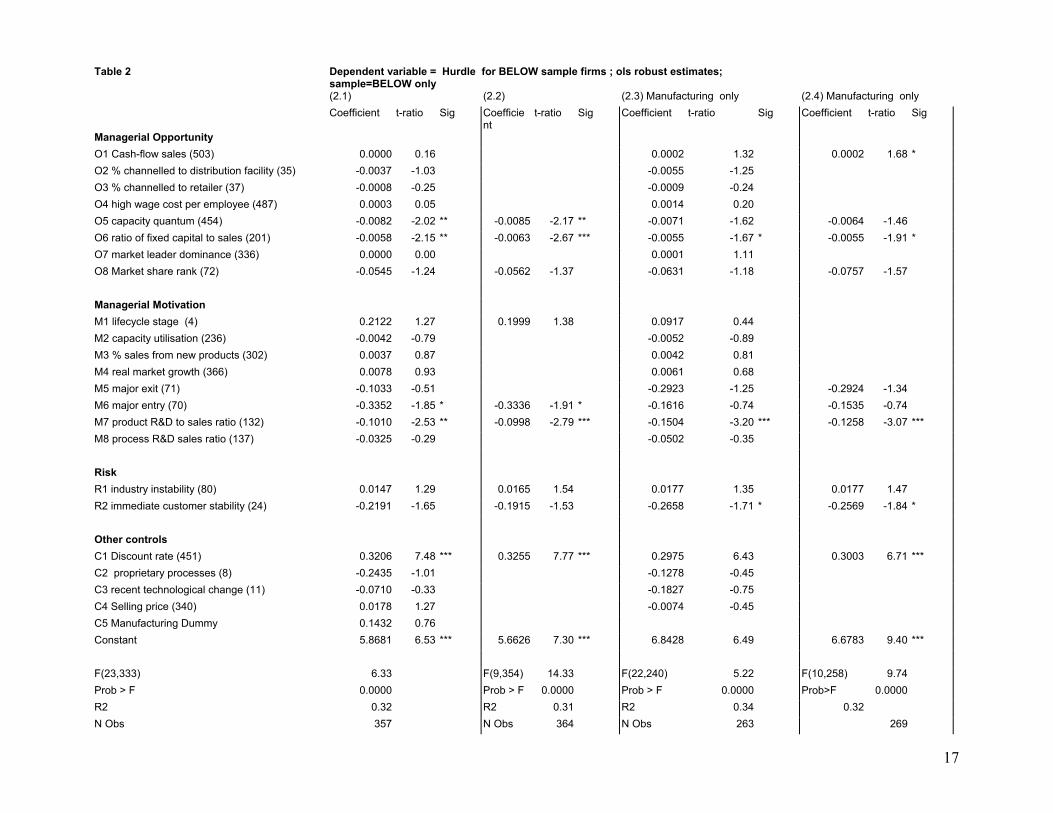
Table 2 Dependent variable = Hurdle for BELOW sample firms ; ols robust estimates;

sample=BELOW only (2.1) (2.2) (2.3) Manufacturing only (2.4) Manufacturing only Coefficient t-ratio Sig Coefficie

nt t-ratio Sig Coefficient t-ratio Sig Coefficient t-ratio Sig

Managerial Opportunity O1 Cash-flow sales (503) 0.0000 0.16 0.0002 1.32 0.0002 1.68 * O2 % channelled to distribution facility (35) -0.0037 -1.03 -0.0055 -1.25O3 % channelled to retailer (37) -0.0008 -0.25 -0.0009 -0.24O4 high wage cost per employee (487) 0.0003 0.05 0.0014 0.20O5 capacity quantum (454) -0.0082 -2.02 ** -0.0085 -2.17 ** -0.0071 -1.62 -0.0064 -1.46O6 ratio of fixed capital to sales (201) -0.0058 -2.15 ** -0.0063 -2.67 *** -0.0055 -1.67 * -0.0055 -1.91 * O7 market leader dominance (336) 0.0000 0.00 0.0001 1.11O8 Market share rank (72) -0.0545 -1.24 -0.0562 -1.37 -0.0631 -1.18 -0.0757 -1.57

Managerial Motivation M1 lifecycle stage (4) 0.2122 1.27 0.1999 1.38 0.0917 0.44M2 capacity utilisation (236) -0.0042 -0.79 -0.0052 -0.89M3 % sales from new products (302) 0.0037 0.87 0.0042 0.81M4 real market growth (366) 0.0078 0.93 0.0061 0.68M5 major exit (71) -0.1033 -0.51 -0.2923 -1.25 -0.2924 -1.34M6 major entry (70) -0.3352 -1.85 * -0.3336 -1.91 * -0.1616 -0.74 -0.1535 -0.74M7 product R&D to sales ratio (132) -0.1010 -2.53 ** -0.0998 -2.79 *** -0.1504 -3.20 *** -0.1258 -3.07 *** M8 process R&D sales ratio (137) -0.0325 -0.29 -0.0502 -0.35

Risk R1 industry instability (80) 0.0147 1.29 0.0165 1.54 0.0177 1.35 0.0177 1.47R2 immediate customer stability (24) -0.2191 -1.65 -0.1915 -1.53 -0.2658 -1.71 * -0.2569 -1.84 *

Other controls C1 Discount rate (451) 0.3206 7.48 *** 0.3255 7.77 *** 0.2975 6.43 0.3003 6.71 *** C2 proprietary processes (8) -0.2435 -1.01 -0.1278 -0.45C3 recent technological change (11) -0.0710 -0.33 -0.1827 -0.75C4 Selling price (340) 0.0178 1.27 -0.0074 -0.45C5 Manufacturing Dummy 0.1432 0.76 Constant 5.8681 6.53 *** 7.305.6626 *** 6.8428 6.49 6.6783 9.40 ***

F(23,333) 6.33 F(9,354) F(22,240)14.33 5.22 F(10,258) 9.74Prob > F 0.0000 Prob > F 0.0000 Prob > F 0.0000 Prob>F 0.0000R2 0.32 R2 R20.31 0.34 0.32N Obs 357 N Obs 364 N Obs 263 269

17

Table 3 Dependent variable = Hurdle for ABOVE Sample firms; ols robust estimates; sample= ABOVE firms only (3.1) (3.2) (3.3) Manufacturing only (3.4) Manufacturing only Coefficient t-ratio Sig Coefficient t-ratio Sig Coefficient t-ratio Sig Coefficient t-ratio Sig

Managerial Opportunity O1 Cash-flow sales (503) -0.0003 -2.06 ** -0.0002 -1.93 * -0.0002 -1.29O2 % channelled to distribution facility (35) 0.0268 2.08 ** 0.0266 1.96 * 0.0354 1.67 * 0.0383 1.82 * O3 % channelled to retailer (37) -0.0047 -1.09 -0.0049 -1.23 -0.0014 -0.25O4 high wage cost per employee (487) -0.0079 -0.77 -0.0215 -1.38 -0.0215 -1.45O5 capacity quantum (454) 0.0059 0.80 0.0148 1.64 0.0161 2.00 ** O6 ratio of fixed capital to sales (201) -0.0043 -1.28 -0.0036 -0.81O7 market leader dominance (336) 0.0003 3.03 *** 0.0003 2.96 *** 0.0003 2.71 *** 0.0004 2.94 *** O8 Market share rank (72) 0.2021 2.34 ** 0.2068 2.52 ** 0.3551 3.21 *** 0.3850 3.96 ***

Managerial Motivation M1 lifecycle stage (4) 0.6752 2.31 ** 0.5923 2.37 ** 1.1054 2.93 *** 1.1382 3.33 *** M2 capacity utilisation (236) 0.0010 0.14 - - 0.0168 1.71 * 0.0156 1.65M3 % sales from new products (302) -0.0189 -2.61 ** -0.0187 -2.86 *** -0.0114 -1.17 - - M4 real market growth (366) 0.0298 2.27 ** 0.0282 2.10 ** 0.0511 2.65 *** 0.0513 2.70 *** M5 major exit (71) -0.2587 -0.83 - - -0.4438 -1.08M6 major entry (70) 1.0987 3.21 *** 1.2130 3.49 *** 1.2248 2.82 *** 1.1366 2.72 *** M7 product R&D to sales ratio (132) 0.1105 1.53 0.1158 1.80 * 0.1467 1.72 * 0.1382 2.05 ** M8 process R&D sales ratio (137) -0.3114 -2.34 ** -0.2878 -2.31 ** -0.2753 -1.52 - -

Risk R1 industry instability (80) 0.0119 0.78 0.0118 0.83 0.0159 0.81 0.0155 0.91R2 immediate customer stability (24) -0.2777 -1.38 0.2482 -1.33 -0.4399 -1.64 -0.4420 -1.71 *

Other controls C1 Discount rate (451) 1.0453 11.01 *** 1.0690 12.53 *** 1.1090 9.71 *** 1.1531 10.29 *** C2 proprietary processes (8) 0.7914 1.54 - - 1.0329 1.76 0.9907 1.73 * C3 recent technological change (11) -0.2825 -0.91 - - -0.0787 -0.20C4 Selling price (340) 0.0522 2.30 ** 0.0474 2.00 ** 0.0662 2.03 ** 0.0819 2.72 *** C5 Manufacturing Dummy 1.4219 4.54 *** 1.2088 3.79 *** - -

Constant -1.1836 -0.80 -1.2692 -0.96 -3.29-3.2859 *** -4.4666 -3.80 ***

F(23,264) 24.64 F(16,279) 21.55 F(22,179) 26.34 F(15,189) 34.88Prob > F 0.0000 Prob > F 0.0000 Prob > F 0.0000 Prob > F 0.0000R2 0.61 R2 0.60 R2 0.63 R2 0.63N Obs 288 N Obs 296 202 N Obs 205

18

7. Discussion of Results for the Separate samples

The relationship between hurdle rates and discount rates: strategists

In the second stage of our empirical analysis, we attempt to unravel the nature of the

relationship between hurdle and discount rates, conducting the investigation on the basis of

different samples (BELOW for the “strategist” firms, ABOVE for the profit maximising firms).

Since our ability to discriminate is less than perfect however, it is important that we still try to

control for possible managerial influences in both sample sets.

Table 2 sets out the results for the BELOW sample (interpreted as managerial empire builders

under H1 or strategists under H2). Variable sets are identical to Table 1. All estimates are now

based on OLS estimators for the hurdle rate (451 – whose definition was discussed above). We

report Huber/White robust estimates of variance. Again we report sensitivity tests by considering

manufacturing alone, although note here we do not see a significant dummy for manufacturing

when the full sample is used.

Our first observation is that in regard to the opportunity set, the fixed capital barrier to entry

variables are again significant (equations 2.1 and 2.2) – although this result is weaker for the

manufacturing firms alone (equations 2.3 and 2.4).

Turning to motivational factors the key result is that the product R&D to sales ratio is highly

significant and negative in all equations – with a rather larger and highly significant coefficient

estimated for manufacturing alone. Put differently, product R&D intensity appears to indicate the

presence of a real option that encourages firms to set hurdle rates with negative expected

return. There is some rather weak evidence that the BELOW sample may act aggressively (loss-

making) in the face of major entry. See the impact of variable 70 (major entry) in 2.1 and 2.2.

However this was not supported within manufacturing.

Overall, these results – especially the significance of product R&D - do not suggest that the

motivation for “over-investment” in this sample is purely of the managerial kind identified by

Jensen (1993). Note that in this regard the cash-flow sales ratio was never significant in our

tests, although perversely, it appears with a marginally (10%) significant positive sign in

manufacturing.

19

Risk factors appear to increase the hurdle rate – with variable 24 (immediate customer stability)

lowering it and variable 80 (industry instability) increasing it, but a conventional F-test on their

joint significance reveals that they are significant at the 5% level only for equation 2.418

Finally, in regard to controls, the coefficient on the discount rate (robustly determined at around

0.3 in all our equations) suggests that capital market influences on the discount rate have only

an attenuated influence on hurdle rates for this sample.

The relationship between hurdle rates and discount rates: profit maximisers

Table 3 examines the relationship between hurdle rates and discount rates for the ABOVE

sample. Three key differences between these results and those reported in table 2 stand out:

First we can see that the discount rate – whose coefficient is insignificantly different from unity -

in all the experiments - now has a one-for-one impact on the hurdle rate, suggesting that these

managers approximate to text-book profit maximisers.

Second, we also note that the free cash flow variable tends to lower the hurdle rate for the full

sample. This may be evidence that this group is subject to the “lemons” problem caused by

asymmetric information between external financiers and industry. Indeed this putative financial

pressure receives some support from the results for the motivation set where actual outcomes in

the development of new products (302) lowers the hurdle – at least in the full sample - but R&D

commitment to products raises it. Put differently, external capital markets may be able to

appraise (highly visible) new products but are unable to appraise R&D devoted to new products

as anything other than as a risk factor.

Third, we also see in the motivation set a very strong result for new entry but the response here

is now accommodating in contrast with the response reported in Table 2. We have seen from

Table 1 that this group of firms has lower scale-related entry barriers and higher capacity

utilisation that the strategist group. It also has faster growth and a higher degree of recent

technological change. These are classic conditions for accommodating entry to be profit

maximising (Besanko, Dranone and Shanley 2000, p.330).

18 A full set of results for F-tests on the variables we have grouped in Tables 2 and 3 is shown in Table 4 below.

20

Some significant variables are perversely signed in this set. For example it is hard to understand

why firms with sales mediated by distributors (presumably meaning less customer pressure)

should have a higher hurdle rate; similarly for the life-cycle variable. It may well be that for this

sample such variables should be more properly regarded as controls since we do not have a

strong prior of strategic or managerial behaviour for this group of businesses. More surprisingly

perhaps, is that we do not find in the first two columns of Table 3 any evidence for the existence

of an irreversibility premium: neither our capital intensity nor our capacity quantum variables

turned out to be significant in the complete specification for the full sample (3.1), and are not

retained in the parsimonious results (3.2). However the manufacturing dummy is highly

significant for this group, suggesting that attention should be paid to equations (3.3) and (3.4)

where we restrict experiments to cases where the firm is identified as belonging to

manufacturing. Most of the results remain robust across equations but some differences need to

be noted:

i) Capacity quantum (v454) which we interpret here as a measure of irreversibility (rather

than a barrier to entry) now comes out as significant and positive as predicted by the

options literature as described above.19 However, the predicted impact is not large. A one

standard deviation change (see Data Appendix) change in this variable produces, on the

basis of (3.4) about 1/3 of a percentage point on the hurdle rate.

ii) The positive impact of product R&D on the hurdle rate appears to be strengthened

iii) The cash flow - sales ratio no longer has a negative impact at conventional levels of

significance.

Further comparisons

To conclude these results it is useful to consider joint tests of significance on the factors

influencing the hurdle rate that we have grouped under the headings of opportunity, motivation

and risk. These are shown in Table 4. At least for our preferred (parsimonious) specifications

the table shows that both the opportunity and motivational sets are important for both sets of

firms; risk factors on the other hand are perhaps surprisingly, statistically significant only for the

BELOW sample . However, immediate customer stability is significant on its own at the 10%

level and correctly signed for manufacturing, in the ABOVE sample.

19 The variable was interpreted as a barrier to entry when discussing the behaviour of strategists but is more properly regarded here as an index of sunk cost or irreversibility.

21

Table 4 F-Tests on Grouped Variables

Managerial Managerial Risk Other

Equation Opportunity Motivation Controls

2.1 F( 8,333) = 1.91

F(8, 333) = 1.86

F( 2,333) = 2.42

F( 5,333) = 12.76

(Prob>F) 0.0570 0.0635 0.0903 0.0000 2.2 F(3,354) = 5.60 F( 3,354) =

5.75 F( 2,354) = 2.69

F( 1,354) = 60.33

(Prob>F) 0.0009 0.0008 0.0696 0.0000 2.3 F( 8,240) =

2.14 F( 8,240) = 1.73

F( 2,240) = 2.57

F(4, 240) = 11.34

(Prob>F) 0.0333 0.0918 0.0783 0.0000 2.4 F(4,258) = 3.40 F(3, 258) =

4.22 F(2, 258) = 3.39

F(1, 258) = 44.98

(Prob>F) 0.0099 0.0062 0.0353 0.0000 3.1 F(8,264) = 3.84 F( 8, 264) =

4.31 F(2, 264) = 1.16

F( 5,264) = 40.31

(Prob>F) 0.0003 0.0001 0.3162 0.0000 3.2 F( 5, 279) =

4.75 F( 6, 279) = 5.69

F(2,279) = 1.15

F(3,279) = 54.90

(Prob>F) 0.0003 0.0000 0.3169 0.0000 3.3 F( 8, 179) =

5.75 F(8,179) = 4.21 F(2, 179) =

1.50 F(4, 179) = 30.99

(Prob>F) 0.0000 0.0001 0.2249 0.0000 3.4 F( 5,189) =

7.37 F( 5,189) = 5.13

F(2,189) =1.73 F(3, 189) = 50.12

(Prob>F) 0.0000 0.0002 0.1802 0.0000

Overall our results in Table 4 suggest that there are important differences between the BELOW

and the ABOVE samples, with the BELOW sample having both the opportunity and the

motivation to pursue investments with a strategic value. We find evidence for both H1 and H2,

and limited evidence for H3, which is strongest for manufacturing.

Two further F-tests are worth reporting here. Modern option theory suggests that a combination

of factors should determine the importance of irreversibility for the investment decision (Chirinko

and Schaller 2002) i.e. low growth, low depreciation, high uncertainty plus a limited resale

market. In our data set these may respectively be proxied by the variables for real market

growth, % sales from new products (negatively), industry instability and capacity quantum. F

tests on the joint significance of these variables for equations 3.1 and 3.3 of Table 3 (where all

22

these variables appear) are significant at 1% and 5% respectively20. On the basis of 3.1, a firm

in an industry where each of these variables was one standard deviation above (below in the

case of % sales from new products) the mean would have a hurdle rate about 1 percentage

point above that for a firm at the mean for these variables.

8. Summary and Conclusions

In this paper we have looked at the relationship between hurdle rates and discount rates to infer

the influence on investment behaviour of a range of firm characteristics. Beginning with the

observation that there are a significant number of firms in our data for whom reported hurdle

rates are below discount rates, we argued that this could be explained by managerialism and/or

the existence of strategic options. Using a probit analysis we found that indicators of likely

managerial and strategic behaviour proved useful to discriminate between firms with hurdle rates

below their discount rate, and firms with hurdle rates above their discount rate. Our results

confirmed that there is quite striking heterogeneity across firms and that this can be explained in

terms of the opportunity and motivation for firms to act strategically.

We then considered the relationship between hurdle rates and discount rates for these two

groups of firms, separately.

For the group of strategist firms it appears that barriers to entry and the strategic value of

investments explain much of the variation in hurdle rates below discount rates. Proxies for entry

barriers such as capital intensity and the lumpiness of investments tend to reduce hurdle rates

for a given discount rate. The same is true of a major indicator of strategic opportunity, viz. the

intensity of product R&D. Moreover the hurdle rate is less responsive to the discount rate than it

is for our second group of firms, which we hypothesise to be classic profit maximisers.

The regression analysis for the second group of firms - which reported hurdle rates above

discount rates - revealed some other important contrasts with the strategists. One such contrast

is in regard to the response to new entry. There is some evidence of an aggressive response

from the strategist sample whereas the profit maximisers tended to pursue an accommodating

approach. The other key contrast is in the impact of product R&D which tends to be associated

20 For equation 3.1 F(4,262) = 3.42 (with Prob>F =0.0095); for equation 3.2 F(4,179) = 2.64 (with Prob>F = 0.0331)

23

with positive strategic value in our first group of firms (and hence a lower hurdle rate) but with a

higher hurdle rate in our second group of firms, perhaps reflecting exposure to risk.

Modern investment theory places a lot of stress on the impact of irreversibility on hurdle rates.

Our search for an irreversibility premium had some success, since indicators of risk helped to

discriminate between the groups. Also, for our second group we found a positive impact on

hurdle rates which emanated from our measure of the size of sunk costs. Moreover, variables

noted in the literature as likely to represent the conditions for real options effects to exist, were

jointly significant at the 1% (5%) level for all industries (manufacturing). However, on this

evidence, the effect may be less important than other factors (such as determinants of the

managerial styles of firms) which clearly have a key influence on the ways in which investment

projects are evaluated.

References: Abel A.B and J.C.Eberly (1994) “A unified model of investment under uncertainty”, American

Economic Review 84, 1369-1384

Abel, A,.B., A.K. Dixit, J.C.Eberly, and R.S.Pindyck (1996) "Options, the Value of Capital and

Investment", Quarterly Journal of Economics August, 753-777

Bunch D.S. and Smiley R. (1992) “Who deters entry? Evidence on the use of strategic entry

deterrents” , Review of Economics and Statistics, 74:3, 509-21

Buzzell R. and B.T. Gale (1987) The PIMS principles: linking strategy to performance, New York,

The Free Press

Chirinko R.S. and Schaller H (2002) “The irreversibility premium” paper given to the American

Economic Association annual conference, Atlanta, January.

Copeland, T., T.Koller and J. Murfin (2000) Valuation: measuring and managing the value of

companies,New York, Wiley (3rd edn)

24

Dixit, A and R. Pindyck (1994) Investment under uncertainty, Princeton: Princeton University

Press

Dixit A. (1981) “The role of investment in entry deterrence”, Economic Journal 90, 95-1006

Geroski, P.A. (1995) “What do we know about entry?”, International Journal of Industrial

Organisation 13, 421-40

Hayes R.H. and Garvin D.A. (1982) “Managing as if tomorrow mattered”, Harvard Business

Review, 60(3), 70-79

Jensen, M.C. (1986) “Agency costs of free cash flow, corporate finance and take-overs”

American Economic Review, 76, 323-329

Jensen, M.C. (1993) “The modern industrial revolution, exit and the failure of internal control

systems”, Journal of Finance 48:3, 831-880

Kaplin R.S. (1986) “Must CIM be justified by faith alone”, Harvard Business Review, 64(2) 87-95

Kathuria, R. and Mueller, D.C. (1995) "Investment and Cash Flow: Asymmetric Information or

Mangerial Discretion" Empirica, 22: 211-234.

Marris, R.L. (1964) The economic theory of managerial capitalism, London,: Macmillan

Morris, D (1998) The stockmarket and the problems of corporate control in the United Kingdom

in T. Buxton, P.Chapman and P.Temple Britain’s Economic Performance, London, Routledge,

200-252

Odagiri, H. (1981) Theory of growth in a corporate economy: management preference, research

and devlopment and economic growth, Cambridge University Press, Cambridge.

Peck, S and Temple, P (1999) “Corporate governance, investment, and economic performance”

in Driver, C and Temple P (eds) Investment, Growth and Employment: Perspectives for Policy,

London: Routledge

25

Odagiri, H. (1992) Growth through competition, competition through growth: strategic

management and the economy in Japan. Clarendon Press, Oxford.

Poterba and Summers (1995) Sloan Management Review, Fall, 43-53

Schwartz E.S. and L. Trigeorgis (2001) Real Options and Investment under Uncertainty:

classical readings and recent contributions, MIT Press

Short, H. (1994) “Ownership, control, financial structure and the performance of firms” Journal of

Economic Surveys, 8(3), 203-245.

Singh S., Utton, M and Waterson, M.(1998) “Strategic behaviour of incumbent firms in the UK”,

International Journal of Industrial Organisation16, 229-51

26

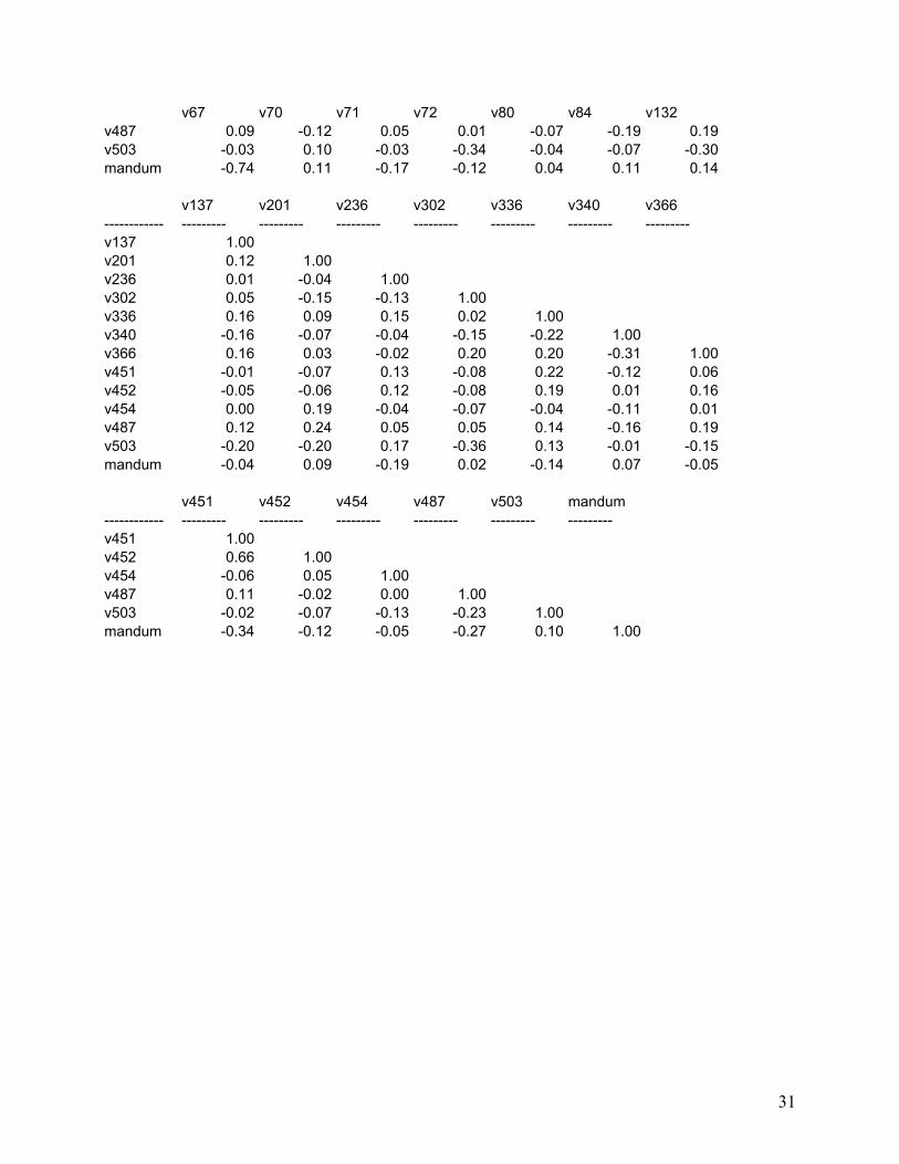
DATA APPENDIX Summary data are described here according to variable numbers as defined in the text. The only variable not appearing there is v67 – which is a four digit SIC code. Table A1 presents summary statistics for the variables deployed in the text based on the sub-samples BELOW and ABOVE. Tables A2 and A3 present correlation matrices for these subsamples. Table A1 Summary Statistics

BELOW Sample ABOVE Sample

Variable Obs Mean Std. Dev. Min Max Obs Mean Std. Dev. Min Max ------------ -------- ------------ ----------- ----------

- -----------

-------- ------------ ----------- -----------

-----------

v4 503 2.86 0.48 1 4 449 2.81 0.54 1 4v8 503 0.20 0.40 0 1 448 0.19 0.39 0 1v11 484 0.26 0.44 0 1 438 0.28 0.45 0 1v24 483 1.84 0.65 1 3 437 1.80 0.65 1 3v35 504 6.14 17.66 0 100 450 5.06 16.53 0 100v37 504 14.38 27.89 0 100 450 19.18 32.07 0 100v67(SIC) 297 3228.48 942.12 1455 9999 239 3352.93 885.54 2010 7512v70 504 0.21 0.41 0 1 446 0.21 0.41 0 1v71 503 0.17 0.38 0 1 443 0.15 0.36 0 1v72 505 2.53 1.92 1 10 452 2.71 2.18 1 10v80 374 10.47 8.65 0.02 40 311 12.24 10.44 0.03 40v84 400 6.36 10.33 0 95 332 5.26 7.96 0 53v132 504 1.42 1.88 0 9 452 1.77 2.24 0 9v137 504 0.50 0.78 0 4 452 0.54 0.83 0 4v201 505 47.21 32.73 3 170 452 46.03 34.21 3 170v236 502 75.98 15.98 30 110 452 75.80 16.28 30 110v302 502 8.48 16.47 0 90.8 446 10.87 19.20 0 99v336 498 2081.23 1356.00 100 6000 445 2045.27 1397.81 100 6000v340 504 7.88 6.28 -5 30 452 7.86 6.73 -5 30v366 502 3.64 10.40 -20 40 452 3.87 11.38 -20 40v451 505 13.97 2.74 8 20 452 9.99 2.69 2 18v452 505 9.87 1.90 4 19 452 13.29 3.62 5 20v454 499 19.31 21.98 0 100 430 17.71 20.33 0 100v487 501 30.54 15.81 5 95 452 28.52 16.06 5 95v503 505 186.12 750.08 -3916 2653.2 452 -22.76 1096.45 -6000 3360mandum 505 0.55 0.50 0 1 452 0.50 0.50 0 1

27

Table A2 BELOW Sample correlation matrix v452 v4 v8 v11 v24 v35 v37

------------ --------- --------- --------- --------- --------- --------- --------- v452 1.00 v4 0.09 1.00 v8 -0.15 -0.38 1.00 v11 -0.05 -0.25 0.40 1.00 v24 -0.13 -0.19 0.16 -0.01 1.00 v35 -0.09 0.01 -0.02 0.06 0.05 1.00 v37 -0.02 0.15 -0.03 -0.11 -0.19 -0.05 1.00 v67 0.14 -0.08 0.07 0.01 0.13 0.00 -0.16 v70 -0.07 -0.13 -0.04 0.01 -0.05 0.03 0.01 v71 -0.11 -0.04 -0.02 -0.01 0.00 0.03 0.03 v72 -0.14 -0.11 0.07 0.06 0.12 -0.02 0.14 v80 0.15 -0.11 -0.04 0.00 0.12 -0.02 -0.08 v84 0.11 0.15 0.00 -0.05 -0.04 -0.01 0.02 v132 -0.19 -0.34 0.30 0.13 0.12 -0.08 -0.10 v137 -0.07 -0.24 0.28 0.14 -0.03 -0.02 -0.13 v201 -0.11 0.00 0.16 -0.02 0.09 -0.13 -0.11 v236 0.04 0.09 0.01 -0.10 -0.05 -0.06 -0.04 v302 -0.04 -0.19 0.11 0.20 0.04 -0.04 0.08 v336 0.06 -0.01 0.18 0.06 -0.07 0.02 -0.10 v340 -0.05 0.06 0.01 0.00 0.01 0.02 -0.09 v366 0.10 -0.22 -0.09 -0.01 0.00 0.02 -0.05 v451 0.46 -0.11 -0.02 0.06 0.01 -0.13 -0.06 v452 1.00 0.09 -0.15 -0.05 -0.13 -0.09 -0.02 v454 -0.06 -0.05 -0.04 -0.02 -0.08 -0.05 0.05 v487 -0.07 -0.22 0.27 0.13 0.18 -0.01 -0.24 v503 0.17 0.09 -0.04 -0.10 -0.04 -0.03 -0.02 mandum -0.07 -0.01 -0.01 0.06 0.03 0.06 0.03

v67 v70 v71 v72 v80 v84 v132

------------ --------- --------- --------- --------- --------- --------- --------- v67 1.00 v70 -0.04 1.00 v71 -0.10 0.26 1.00 v72 -0.08 -0.10 -0.06 1.00 v80 0.34 -0.05 0.00 0.05 1.00 v84 0.00 -0.06 -0.09 -0.01 -0.15 1.00 v132 0.17 0.06 -0.07 0.12 0.10 -0.08 1.00 v137 -0.01 0.01 -0.02 0.04 -0.02 -0.03 0.23 v201 -0.17 -0.05 -0.02 0.06 -0.11 0.00 -0.05 v236 -0.05 -0.09 -0.06 -0.12 -0.07 -0.01 -0.19 v302 0.00 0.07 -0.04 0.07 0.09 -0.01 0.32 v336 -0.17 0.09 0.01 -0.24 -0.16 0.13 0.14 v340 -0.11 0.02 0.09 0.00 -0.07 0.00 -0.15 v366 0.17 0.06 -0.06 -0.02 0.11 -0.10 0.12 v451 0.06 0.01 -0.08 -0.04 0.10 -0.04 -0.05 v452 0.14 -0.07 -0.11 -0.14 0.15 0.11 -0.19 v454 -0.16 0.09 0.08 -0.05 -0.17 -0.07 0.03

28

v67 v70 v71 v72 v80 v84 v132 v487 0.02 0.03 0.04 0.09 -0.04 -0.08 0.12 v503 0.14 -0.03 -0.02 -0.12 0.06 0.05 -0.10 mandum -0.41 0.03 0.08 0.00 -0.29 0.13 0.12

v137 v201 v236 v302 v336 v340 v366

------------ --------- --------- --------- --------- --------- --------- --------- v137 1.00 v201 0.20 1.00 v236 0.10 0.16 1.00 v302 0.19 -0.13 -0.04 1.00 v336 0.18 0.02 0.07 0.10 1.00 v340 -0.06 0.08 0.13 -0.07 0.11 1.00 v366 0.07 -0.02 0.01 0.03 0.05 -0.18 1.00 v451 0.11 0.08 0.08 -0.02 0.11 -0.05 0.16 v452 -0.07 -0.11 0.04 -0.04 0.06 -0.05 0.10 v454 0.16 0.08 -0.03 0.06 0.15 0.00 0.14 v487 0.20 0.27 0.02 -0.05 0.10 0.08 0.00 v503 -0.24 -0.08 0.07 -0.12 0.07 0.04 0.04 mandum 0.01 0.00 -0.10 0.04 0.08 0.01 -0.14

v451 v452 v454 v487 v503 mandum

------------ --------- --------- --------- --------- --------- --------- v451 1.00 v452 0.46 1.00 v454 0.10 -0.06 1.00 v487 0.02 -0.07 -0.02 1.00 v503 0.02 0.17 -0.08 -0.01 1.00 mandum -0.03 -0.07 0.08 -0.13 0.03 1.00

29

Table A3 ABOVE Sample correlation matrix

v452 v4 v8 v11 v24 v35 v37 ------------ --------- --------- --------- --------- --------- --------- --------- v452 1.00 v4 0.11 1.00 v8 0.23 -0.30 1.00 v11 0.15 -0.31 0.27 1.00 v24 -0.12 0.09 -0.03 0.00 1.00 v35 -0.01 0.04 -0.02 -0.03 0.09 1.00 v37 0.08 0.15 -0.06 -0.13 -0.09 -0.04 1.00 v67 0.22 -0.09 0.20 0.15 -0.05 -0.01 -0.12 v70 0.06 -0.15 0.07 0.04 -0.04 0.05 -0.12 v71 -0.05 0.04 0.02 0.01 0.02 0.07 -0.06 v72 0.07 0.01 -0.04 -0.05 0.09 -0.02 0.02 v80 -0.04 -0.05 -0.08 -0.05 -0.04 -0.05 0.17 v84 0.06 0.11 -0.16 0.00 0.21 -0.07 -0.18 v132 0.09 -0.19 0.22 0.16 0.19 -0.10 -0.32 v137 -0.05 -0.21 0.19 0.13 -0.03 -0.10 -0.17 v201 -0.06 -0.10 0.21 0.16 -0.01 -0.05 -0.09 v236 0.12 0.08 -0.01 0.10 -0.03 0.13 -0.04 v302 -0.08 -0.28 0.04 0.08 0.05 0.00 -0.09 v336 0.19 -0.12 0.25 0.19 -0.12 -0.11 0.01 v340 0.01 0.19 -0.24 -0.09 0.06 0.02 0.08 v366 0.16 -0.35 0.22 0.21 -0.02 0.01 -0.03 v451 0.66 0.05 0.26 0.23 -0.16 -0.21 0.14 v452 1.00 0.11 0.23 0.15 -0.12 -0.01 0.08 v454 0.05 -0.06 0.07 0.10 0.07 0.15 -0.04 v487 -0.02 -0.04 0.25 0.26 0.00 0.01 -0.01 v503 -0.07 0.24 -0.13 -0.17 -0.01 0.01 0.11 mandum -0.12 0.06 -0.26 -0.14 0.20 0.01 -0.08

v67 v70 v71 v72 v80 v84 v132 ------------ --------- --------- --------- --------- --------- --------- --------- v67 1.00 v70 0.03 1.00 v71 0.10 -0.09 1.00 v72 0.00 -0.16 0.02 1.00 v80 -0.08 0.08 -0.10 0.03 1.00 v84 0.11 0.02 0.12 -0.01 -0.13 1.00 v132 0.08 0.20 -0.05 -0.14 -0.01 0.28 1.00 v137 0.19 0.18 -0.05 -0.08 0.10 0.00 0.13 v201 -0.24 -0.10 -0.10 0.00 -0.05 -0.09 0.10 v236 0.28 -0.07 0.03 -0.12 -0.04 0.00 -0.13 v302 0.05 0.17 0.11 0.00 0.03 0.17 0.47 v336 0.22 0.02 -0.10 -0.41 -0.03 0.00 0.26 v340 -0.13 0.02 -0.12 0.12 0.07 0.04 -0.21 v366 0.09 0.23 -0.03 -0.06 -0.04 -0.10 0.19 v451 0.39 -0.15 0.07 -0.09 -0.12 0.03 0.03 v452 0.22 0.06 -0.05 0.07 -0.04 0.06 0.09 v454 -0.11 -0.01 -0.01 0.16 -0.04 -0.12 -0.10

30

31

v67 v70 v71 v72 v80 v84 v132 v487 0.09 -0.12 0.05 0.01 -0.07 -0.19 0.19 v503 -0.03 0.10 -0.03 -0.34 -0.04 -0.07 -0.30 mandum -0.74 0.11 -0.17 -0.12 0.04 0.11 0.14

v137 v201 v236 v302 v336 v340 v366

------------ --------- --------- --------- --------- --------- --------- --------- v137 1.00 v201 0.12 1.00 v236 0.01 -0.04 1.00 v302 0.05 -0.15 -0.13 1.00 v336 0.16 0.09 0.15 0.02 1.00 v340 -0.16 -0.07 -0.04 -0.15 -0.22 1.00 v366 0.16 0.03 -0.02 0.20 0.20 -0.31 1.00 v451 -0.01 -0.07 0.13 -0.08 0.22 -0.12 0.06 v452 -0.05 -0.06 0.12 -0.08 0.19 0.01 0.16 v454 0.00 0.19 -0.04 -0.07 -0.04 -0.11 0.01 v487 0.12 0.24 0.05 0.05 0.14 -0.16 0.19 v503 -0.20 -0.20 0.17 -0.36 0.13 -0.01 -0.15 mandum -0.04 0.09 -0.19 0.02 -0.14 0.07 -0.05

v451 v452 v454 v487 v503 mandum

------------ --------- --------- --------- --------- --------- --------- v451 1.00 v452 0.66 1.00 v454 -0.06 0.05 1.00 v487 0.11 -0.02 0.00 1.00 v503 -0.02 -0.07 -0.13 -0.23 1.00 mandum -0.34 -0.12 -0.05 -0.27 0.10 1.00