INVESTING IN POWER GRID

INTERCONNECTION IN EAST ASIA

INVESTING IN POWER GRID INTERCONNECTION IN EAST ASIA

Edited by

ICHIRO KUTANI AND YANFEI LI

Economic Research Institute for ASEAN and East Asia

DDIISSCCLLAAIIMMEERR

This report was prepared by the Working Group for the Sustainable Development of the Natural Gas Market in the East Asia Summit (EAS) Region under the Economic Research Institute for ASEAN and East Asia (ERIA) Energy Project. Members of the Working Group, who represent the participating EAS region countries, discussed and agreed to utilize certain data and methodologies proposed by the Institute of Energy Economics, Japan (IEEJ) to analyse market trends. These data and methodologies may differ from those normally used in each country. Therefore, the calculated result presented here should not be viewed as the official national analyses of the participating countries. The views in this publication do not necessarily reflect the views and policies of the Economic Research Institute for ASEAN and East Asia (ERIA), its Academic Advisory Council, and the Management.

Copyright ©2014 by Economic Research Institute for ASEAN and East Asia

All rights reserved. No part of this publication may be reproduced, stored in a retrieval system, or transmitted, in any form or by any means, electronic, mechanical photocopying, recording or otherwise, without prior notice to or permission from the Publisher.

Book design by Fadriani Trianingsih. ERIA Research Project Report 2013, No.26 Published October 2014

v

CONTENTS

List of Figures vi

List of Tables ix

Foreword x

Acknowledgements xi

List of Project Members xii

List of Abbreviations and Acronyms xiv

Executive Summary xvi

Chapter 1 Introduction 1

Chapter 2 Electric Power Supply in EAS Countries 5

Chapter 3 Optimising Power Infrastructure Development 27

Chapter 4 Preliminary Assessment of Possible Interconnection 51

Chapter 5 Key Findings and Next Step 63

Appendix 1 Power Generation Mix in Each Case (2035) 71

Appendix 2 Power Trade in Each Case (2025, 2030, 2035) 73

Appendix 3 Cumulative Cost Up to 2035 (differences compared to Case 0) 79

vi

LIST OF FIGURES

Figure 1.1 Study flow 4

Figure 2.1 Projected electric power demand (TWh) 6

Figure 2.2 Breakdown of existing power generation capacity as of

2012 (MW)

8

Figure 2.3 Potential of the various energy resources in the countries

of ASEAN

11

Figure 2.4 Projected hydropower development potential in 2035

(TWh)

12

Figure 2.5 Daily load curve (average for 2006) and load duration

curve for BRN

13

Figure 2.6 Daily load curve (dry season, 2013) and load duration

curve for IDN

14

Figure 2.7 Daily load curve (average for 2007) and load duration

curve for KHM

14

Figure 2.8 Daily load curve (dry season, 2012) and load duration

curve for LAO

14

Figure 2.9 Daily load curve (rainy season, 2007) and load duration

curve for MYA

15

Figure 2.10 Daily load curve (June 2012) and load duration curve for

MYS

15

Figure 2.11 Daily load curve (July 2013) and load duration curve for

NEI

15

Figure 2.12 Daily load curve (September 2011) and load duration

curve for PHL

16

vii

Figure 2.13 Daily load curve (May 2010) and load duration curve for

SPG

16

Figure 2.14 Daily load curve (April 2012) and load duration curve for

THA

16

Figure 2.15 Daily load curve (August 2011) and load duration curve

for VNM

17

Figure 2.16 Projected future construction costs (by energy source) 18

Figure 2.17 Projected future variable O&M costs (by energy source) 19

Figure 2.18 Projected thermal efficiency (by energy source) 19

Figure 2.19 Projected future coal prices (Steam coal) 20

Figure 2.20 Projected future natural gas prices 21

Figure 2.21 ASEAN Power Grid (APG) 23

Figure 2.22 Greater Mekong Sub-region (GMS) 24

Figure 3.1 Preconditions and outputs of the optimal power

generation planning model

27

Figure 3.2 Power source choices in the optimal calculations 28

Figure 3.3 Supply reliability evaluation model 31

Figure 3.4 Comparison between the calculation results for each

country’s power generation mix and the ERIA Outlook

33

Figure 3.5 Required reserve margin to gain the same LOLE 36

Figure 3.6 Power supply mix in 2035 (Case 0) 36

Figure 3.7 Power supply mix in 2035 (Case 1) 37

Figure 3.8 Power supply mix in 2035 (Case 2a) 38

Figure 3.9 Power supply mix in 2035 (Case 2b) 39

Figure 3.10 Power supply mix in 2035 (Case 3) 39

Figure 3.11 Power supply mix in 2035 (total of all regions) 40

Figure 3.12 CO2 emissions in 2035 41

Figure 3.13 Power trade flows in 2035 (Case 1) 42

viii

Figure 3.14 Power trade flows in 2035 (Case 2a) 43

Figure 3.15 Power trade flows in 2035 (Case 2b) 44

Figure 3.16 Power trade flows in 2035 (Case 3) 45

Figure 3.17 Changes in power trade in Case 2b (1) 46

Figure 3.18 Changes in power trade in Case 2b (2) 47

Figure 3.19 Changes in power trade in Case 2b (3) 47

Figure 3.20 Changes in power trade in Case 2b (4) 48

Figure 3.21 Cumulative costs in each case 49

Figure 4.1 How routes are considered in each case 52

Figure 4.2 Actual transmission line construction costs in

neighbouring countries (500kV overhead lines)

55

Figure 4.3 Actual transmission line construction costs in

neighbouring countries (500kV undersea cable)

55

ix

LIST OF TABLES

Table 2.1 List of country names and abbreviations 5

Table 2.2 Projected international interconnection transmission

capacity in 2020 and later (GW)

22

Table 4.1 Route length calculation results (Route 1) 53

Table 4.2 Route length calculation results (Route 2) 53

Table 4.3 Transmission line construction costs (Route 1) 59

Table 4.4 Transmission line construction costs (Route 2) 60

Table 4.5 Estimated cost benefit of new transmission line 61

Table 5.1 Possible interconnection and cumulative cost benefit 64

Table 5.2 Cost benefit and equivalent investment 65

Table 5.3 Possible interconnection line and their priority 66

Table 5.4 HAPUA lead plan 67

x

FOREWORD

In East Asian countries where electricity demand is rapidly increasing, there

is a necessity for planting up more generating capacities to meet the growing

demand. At the same time, cheaper electricity will be required when

considering the impact on the general public and economy, and the needs for

cleaner electricity will become stronger when considering impact on pollution

and climate issue.

On the other hand, in East Asian countries, (potential) resources like coal,

natural gas and river to fuel power plants remain underdeveloped. If this

region can utilise these resources, it might be possible to supply sufficient

amount of electricity at cheaper price. Furthermore, energy security is

enhanced through reducing regional import dependency of energy supply.

One possible option to maximise the use of undeveloped resources in the

region is international/regional grid interconnection. The region can optimise

power supply mix through cross-border power transaction.

Against this backdrop, ERIA organised a working group to carry out a study

which aims to analyse a possible optimum power generation mix of the

region, and to provide policy recommendations for the improvement of that

situation. Experts from EAS countries were gathered to discuss their existing

power development plans and possibility for regional optimisation. The result

of their work is this volume titled Investing in Power Grid Interconnection in

East Asia.

It is our hope that the outcome from this work will serve as a reference for

policymakers in East Asian countries and contribute to the improvement of

energy security in the region as a whole.

Prof. Hidetoshi Nishimura

ERIA Executive Director

September 2014

xi

ACKNOWLEDGEMENTS

This analysis has been implemented by a working group under ERIA. It

was a joint effort of Working Group members from the EAS countries and the

IEEJ (The Institute of Energy Economics, Japan). We would like to

acknowledge the support provided by everyone involved. We would

especially like to express our gratitude to the members of the Working Group,

the Economic Research Institute for ASEAN and East Asia (ERIA) and

IEEJ’s study project team.

In addition, I would like to acknowledge Mr. Shaiful Bakhri Ibrahim,

HAPUA Secretary in Charge, for his contribution in providing insights on the

issue that was subject of the study.

Special mention and recognition should also be given to the authors of one of

the chapters of this report:

Chapter 4 by Mr. Yoichiro Kubota and Mr. Noboru Seki of

Tokyo Electric Power Company.

Mr. Ichiro Kutani

Leader of the Working Group

September 2014

xii

LIST OF PROJECT MEMBERS

Working Group Members

MR. ICHIRO KUTANI (LEADER): Senior Economist, Manager, Global Energy

Group 1 , Assistant to Managing Director, Strategy Research Unit, The

Institute of Energy Economics, Japan (IEEJ)

MR. SHIMPEI YAMAMOTO (ORGANIZER): Managing Director for Research

Affairs, Economic Research Institute for ASEAN and East Asia (ERIA)

MR. SHIGERU KIMURA (ORGANIZER): Special Advisor to Executive Director

on Energy Affairs, Economic Research Institute for ASEAN and East

Asia (ERIA)

DR. HAN PHOUMIN (ORGANIZER): Energy Economist, Energy Unit, Research

Department, Economic Research Institute for ASEAN and East Asia

(ERIA)

DR. ANBUMOZHI VENKATACHALAM (ORGANIZER): Energy Economist,

Energy Unit, Research Department, Economic Research Institute for

ASEAN and East Asia (ERIA)

DR. YANFEI LI (ORGANIZER): Energy Economist, Energy Unit, Research

Department, Economic Research Institute for ASEAN and East Asia

(ERIA)

MR. PISETH SOUEM: Officer, General Department of Energy, Ministry of

Mines and Energy (MME), Cambodia

MR. Wong Yuk-sum: Consultant, Automotive and Electronics Division,

Hong Kong Productivity Council (HKPC), China

MR. AWDHESH KUMAR YADAV: Deputy Director, System Planning and

xiii

Project Appraisal Power System, Central Electricity Authority (CEA),

India

MR. PRAMUDYA: Electricity Inspector, Directorate of Electricity Program

Supervision, Directorate General of Electricity, Ministry of Energy and

Mineral Resources (MEMR), Indonesia

MR. WATARU FUJISAKI: Senior Coordinator, Global Energy Group 1,

Strategy Research Unit, The Institute of Energy Economics, Japan

(IEEJ)

MR. YUHJI MATSUO: Senior Economist, Nuclear Energy Group, Strategy

Research Unit, The Institute of Energy Economics, Japan (IEEJ)

MR. KAZUTAKA FUKASAWA: Senior Researcher, Global Energy Group 1,

Strategy Research Unit, The Institute of Energy Economics, Japan

(IEEJ)

MR. BOUNGNONG BOUTTAVONG: Deputy Director, Technical Department,

Electricite Du Laos (EDL), Lao PDR

MR. JOON BIN IBRAHIM: General Manager (Technical Advisory & Industry

Development), Single Buyer Department, Tenaga Nasional Berhad

(TNB), Malaysia

DR. JIRAPORN SIRIKUM: Assistant Director of System Planning Division -

Generation, Electricity Generating Authority of Thailand (EGAT),

Thailand

MR. TANG THE HUNG: Deputy Director, Planning Department, General

Directorate of Energy, Ministry of Industry and Trade (MOIT), Viet

Nam

xiv

LIST OF ABBREVIATIONS AND ACRONYMS

AAGR = Average Annual Growth Rate

AC = Alternating Current

ADB = Asian Development Bank

APG = ASEAN Power Grid

ASEAN = Association of Southeast Asian Nations

BAU = Business as Usual

CO2 = Carbon dioxide

DC = Direct Current

EAS = East Asia Summit

EC = European Commission

ECTF = Energy Cooperation Task Force

EIA = Energy Information Administration

ERIA = Economic Research Institute for ASEAN and East Asia

ETP = Energy Technology Perspectives

GDP = Gross Domestic Product

GMS = Greater Mekong Sub-region

GW = Giga Watt

HAPUA = The Heads of ASEAN Power Utilities/Authorities

IEA = International Energy Agency

IEEJ = The Institute for Energy Economics, Japan

LOLE = Loss of Load Expectation

MOU = Memorandum of Understanding

MW = Mega Watt

O&M = Operation & Maintenance

xv

OECD/NEA = Organisation for Economic Co-operation and Development -

Nuclear Energy Agency

TWh = Tera Watt hour

USD = United States Dollar

WG = Working Group

xvi

EXECUTIVE SUMMARY

This report examines the possibility of improving investment efficiency of

power infrastructures through enhancing interconnection of power grids in

the region, mainly focused on South East Asia.

MAIN ARGUMENT

In general, power infrastructure development is made under the premise of

self-sufficiency within each country. While there remain much resources to

fuel power stations in some countries, other countries are facing difficulties in

their own power development. Power grid interconnections are a possible

option to overcome these challenges. Regional planning of power

infrastructure development is anticipated to provide benefits of total

investment cost reductions, improve electricity supply stability and move

towards decarbonisation.

The study first developed simulation models that enable the analysis of

least-cost mix of power generation and grid interconnection. A second part of

the study estimated the cost of possible interconnection lines which is derived

from the above mentioned simulation analysis. By comparing these two

outcomes, namely, benefit and cost of enhanced grid interconnection, the

report has selected priority projects that seem to provide greater benefit for

the region and at the same time are perceived to be economically viable.

KEY FINDINGS

・ Possible interconnection line, its estimated cost and net economic benefits,

which imply feasibility and priority of the proposed new transmission

capacities, are estimated.

・ A positive net economic benefit indicates economic feasibility of the

project and thus should be prioritised. Among the listed projects, the Viet

Nam - Lao - Thailand – Malaysia – Singapore interconnection route could

be the most beneficial, and the Cambodia - Thailand linkage could be the

xvii

Possible cumulative cost

benefit range

[mil.USD]

Estimated cost of

trasmission line

[mil USD]

A THA-KHM 4,560 -- 5,470 162 -- 1,009 second priority

B THA-LAO 19,282 -- 20,604 728 -- 1,957 first priority

C THA-MYA (4,607) -- (2,766) 2,244 -- 3,956 need careful assess.

D MYA-THA-MYS-SGP (1,118) -- 3,064 2,384 -- 6,272 need careful assess.

E VNM-LAO-THA 21,604 -- 23,715 922 -- 2,885 first priority

F MYS-IDN 3,968 -- 4,087 1,790 -- 1,901 second priority

G LAO-THA-MYS-SGP 23,217-- 26,557 868 -- 4,273 first priority

Case

second beneficial interconnection.

IDN: Indonesia, KHM: Cambodia, LAO: Laos, MYA: Myanmar, MYS: Malaysia,

SGP: Singapore, THA: Thailand, VNM: Viet Nam

* Numbers in brackets are negative.

POLICY IMPLICATIONS

・ If grid interconnections within the region are to be enhanced, investment

efficiency for power infrastructure could be improved. Interconnections

also bring other benefits such as electricity supply stability and reduction of

greenhouse gas emissions.

・ The following are some key challenges that need to be resolved for the

advancement of grid interconnection:

Each power grid is unique and governed by its own policies and

codes. There needs to be a comprehensive guideline

encompassing all the member countries. At the moment, there has

yet to be sufficient bilateral or multilateral discussion and

coordination in order to promote construction.

The investment environment is not always attractive to private

companies and foreign capital. Accordingly, there has not been a

sufficient provision of capital.

1

CHAPTER 1

INTRODUCTION

In the EAS (East Asia Summit) countries, power demand is steadily

expanding due to population increase and economic growth. As improving

the electrification rate is an important policy task in some countries, power

demand appears most certain to increase in the future in line with rising living

standards. Meanwhile, as GDP is relatively low in this region, it is necessary

to supply electricity at the minimum possible cost. Therefore, for the EAS

countries, steadily implementing large-scale power source development in an

economically efficient way is an urgent task.

Basically, a country implements power source development on the premise

of self-sufficiency. That is natural from the perspective of energy security of a

country, and it is a rational approach when demand growth is moderate or the

country can implement economically efficient power source development on

its own so as to meet the demand. However, when demand growth outstrips

the capacity to supply necessary domestic resources (manufacturing, human

and financial resources) or when economically efficient power source

development is difficult due to some constraints, importing electricity from

neighbouring countries should be considered as an option. In light of the

above, it may be possible to optimise or to improve the efficiency of power

infrastructure development in terms of supply stability, economic efficiency

and reduction of the environmental burden if ways of developing power

infrastructures (power sources and grids) on a pan-regional basis are

considered.

This idea may be supported by creating an ASEAN Economic Community

(AEC) by 2015. The initiative is aimed at strengthening regional ties by

enhancing inter-regional trade, including energy commodity.

Meanwhile in the ASEAN region, HAPUA (The Heads of ASEAN Power

Utilities/Authorities ） and the Asian Development Bank (ADB) are

implementing initiatives related to intra-regional power grid interconnections

and, at the same time, bilateral power imports/exports are ongoing. However,

2

some countries are still placing priority on the optimisation of investments at

the domestic level. Besides, power imports and exports are not brisk enough

to contribute to “power grid interconnection,” and progress towards

pan-regional optimisation has been slow.

1.1. Rationale

The rationale of this study is derived from the 17th ECTF1 (Energy

Cooperation Task Force) meeting held in Phnom Penh, Cambodia on 5 July

2012. During this meeting, the Economic Research Institute for ASEAN

and East Asia (ERIA) explained and proposed new ideas and initiatives for

energy cooperation, including the following:

- Strategic Usage of Coal

- Optimum Electric Power Infrastructure

- Nuclear Power Safety Management, and

- Smart Urban Traffic

The participants of the ECTF Meeting exchanged views on the above

proposals and agreed to endorse the proposed new areas and initiatives.

As a result, ERIA has formulated the Working Group for the “Study on

Effective Investment of Power Infrastructure in East Asia through Power Grid

Interconnection”. Members from EAS countries are represented in the WG

with Mr. Ichiro Kutani of the Institute of Energy Economics, Japan (IEEJ) as

the leader of the group.

1.2. Objective

The Working Group’s study, which is packaged in this volume titled

Investing in Power Grid Interconnection in East Asia, quantifies the benefits

of the pan-regional optimisation of power infrastructure development in the

EAS region. By doing so, the study provides clues for improving efficiency

of investment for power station and cross-border grid interconnection. It

should be noted that the background of this study has been developed by

making reference to the Greater Mekong Sub-region (GMS) program of ADB

1 Energy Cooperation Task Force under the Energy Ministers Meeting of EAS countries.

3

and ASEAN Power Grid (APG) program of HAPUA, thus making the study

consistent with these existing initiatives.

1.3. Work stream and working group activity

1.3.1. Fiscal year 2012

In the first year of the study, the following describes the work streams that

were conducted.

(A) Collecting power infrastructure data and information

(B) Identifying challenges and discussion points

(C) Developing a simplified power infrastructure simulation model

(D) Drawing out policy recommendations (preliminary analysis)

In 2012, the WG held two meetings; one in November 2012 in Jakarta,

Indonesia and another in April 2013 in Tokyo, Japan.

In the first meeting, information sharing and discussion regarding each

country's power source development plan took place. Additionally, issues

related to existing initiatives such as the ASEAN Power Grid and GMS were

discussed.

During the second meeting, the validity of data input for simulations of

optimal energy mixes was examined, and calculation results were evaluated

and discussed.

1.3.2. Fiscal year 2013

In the second year of the study, the following work streams were

conducted.

(E) Detailed analysis of optimal power infrastructures

Here, a more detailed simulation model, and exercise analysis to figure out

optimal mix (cost minimum) of power generation and beneficial

interconnection lines were developed. This part of the study provides possible

benefit for each candidate through interconnection.

4

- Annual / daily load curb of demand

- Cost of power generation (construction, O&M, fuel)

- Interconnection line (connecting point, length, capacity, loss rate)

- Cost of interconnection line (construction, O&M)

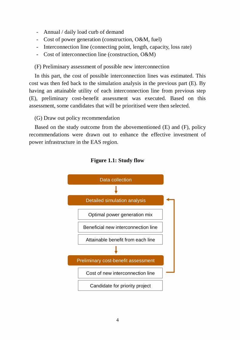
(F) Preliminary assessment of possible new interconnection

In this part, the cost of possible interconnection lines was estimated. This

cost was then fed back to the simulation analysis in the previous part (E). By

having an attainable utility of each interconnection line from previous step

(E), preliminary cost-benefit assessment was executed. Based on this

assessment, some candidates that will be prioritised were then selected.

(G) Draw out policy recommendation

Based on the study outcome from the abovementioned (E) and (F), policy

recommendations were drawn out to enhance the effective investment of

power infrastructure in the EAS region.

Figure 1.1: Study flow

Detailed simulation analysis

Optimal power generation mix

Beneficial new interconnection line

Preliminary cost-benefit assessment

Attainable benefit from each line

Cost of new interconnection line

Candidate for priority project

Data collection

5

CHAPTER 2

ELECTRIC POWER SUPPLY IN EAS COUNTRIES

This chapter sets out the data for each individual country used in the

simulation model (in Chapter 3).

The simulation model covers a total of 12 East Asian countries, namely,

Brunei Darussalam, Cambodia, China (Yunnan Province), India (northeast

region), Indonesia, Lao People’s Democratic Republic (PDR), Malaysia,

Myanmar, the Philippines, Singapore, Thailand and Viet Nam. The following

abbreviations are used in this report to represent the names of these countries.

Table 2.1: List of country names and abbreviations

2.1. Projected electric power demand

The projected power demand for each country was assumed on the basis of

the power generation output (TWh) for each country in the business as usual

(BAU) scenario discussed in the ERIA Research Project Report 2012, No.

19 titled “Analysis on Energy Saving Potential in East Asia”.

However, the projected power demand figures for India (northeast region)

and China (Yunnan Province) were calculated by taking the power generation

output (TWh) of the entire country to which each of the regions belongs, and

calculating a share of this output proportional to the region’s actual

performance in the regional breakdown of the country’s generation output.

Country 3-letter codes Country 3-letter codes

Brunei Darussalam BRN Malaysia MYS

Cambodia KHM Myanmar MYA

China (Yunnan province) YNN Philippines PHL

India (North-East region) NEI Singapore SGP

Indonesia IDN Thailand THA

Lao PDR LAO Vietnam VNM

6

Figure 2.1: Projected electric power demand (TWh)

Source: ERIA Research Project Report 2012,

“Analysis on Energy Saving Potential in East Asia”

The demand for energy in the East Asian region has risen steadily to date,

and is expected to increase continuously forward due to the expansion of the

power supply region, the industrialisation in line with economic growth,

rising income levels, and urbanisation.

With Indonesia, Malaysia, Thailand, Viet Nam and China (Yunnan

Province) showing particularly dramatic increases in demand, it will be

essential to expand and augment all power-related facilities including power

generation, transmission and distribution facilities in all of these countries.

From 2010 to 2035, Indonesia’s power demand is projected to rise from

169.8TWh to 733.1TWh, Malaysia’s from 124.1TWh to 371.8TWh,

Thailand’s from 147.0TWh to 355.0TWh, Viet Nam’s from 92.2TWh to

0

100

200

300

400

500

600

700

800

BRN

IDN

KHM

LAO

MYA

MYS NEI

PHL

SGP

THA

VN

M

YNN

2010 2020 2035

TWh

2010 2015 2020 2025 2030 2035 2010-2020 2020-2035 2010-2035

BRN 3.87 4.47 5.22 5.96 6.77 7.67 3.0% 2.6% 2.8%

IDN 169.79 252.38 341.64 448.07 576.05 733.09 7.2% 5.2% 6.0%

KHM 0.99 6.15 12.33 17.67 19.58 22.15 28.6% 4.0% 13.2%

LAO 8.45 22.54 51.35 65.44 67.13 68.82 19.8% 2.0% 8.8%

MYA 7.54 11.42 16.44 23.15 32.24 44.59 8.1% 6.9% 7.4%

MYS 124.10 161.20 205.10 254.00 309.10 371.80 5.2% 4.0% 4.5%

NEI 11.44 15.68 22.18 29.52 38.34 49.28 6.8% 5.5% 6.0%

PHL 67.74 84.63 106.79 130.51 156.00 185.93 4.7% 3.8% 4.1%

SGP 45.38 51.19 55.60 59.40 61.85 65.76 2.1% 1.1% 1.5%

THA 147.01 180.37 210.86 257.53 309.56 355.03 3.7% 3.5% 3.6%

VNM 92.17 148.35 219.59 295.41 398.83 538.70 9.1% 6.2% 7.3%

YNN 136.50 188.88 223.71 260.19 296.66 324.67 5.1% 2.5% 3.5%

TWh AAGR

7

538.7TWh, and Yunnan Province’s from 249.4TWh to 593.2TWh.

Increases in demand during the period up to 2020 are expected to be

particularly substantial in Cambodia and Lao PDR.

Power demand in Cambodia is forecast to increase by 13.2 percent a year

over the 25-year period from 2010 to 2035, soaring by 28.6 percent a year

over the 10-year period leading up to 2020. Much of Cambodia is still

without electricity, with the country’s electricity supply currently confined

largely to the capital region and major cities. As of June 2012, the household

electrification rate for the country as a whole stood at approximately 35

percent, with the rate for urban areas at almost 100 percent; whereas that for

rural areas was only around 25 percent. Moreover, latent power demand is

believed to be considerable even in regions where power is already supplied,

because the power demand from many of the production plants and hotels

found in these regions are supplied by private power generators. Against this

backdrop, the Government of Cambodia has set out targets of achieving 100

percent village electrification by 2020, and over 70 percent household

electrification by 2030; and aims to improve the state of Cambodia’s power

generation and distribution facilities and ensure an affordable and stable

supply of power.

It is expected that in Lao PDR, power demand will increase as its

manufacturing and commercial industries develop as a result of foreign

investment and as progress is made in policies aiming to increase the

country’s electrification rate. Power demand in Lao PDR is forecast to

increase by 8.8 percent a year over the 25-year period from 2010 to 2035,

soaring by 19.8 percent a year over the 10-year period leading up to 2020.

The Government of Lao PDR has set out a target of raising the household

electrification rate in Lao PDR to 90 percent by 2020.

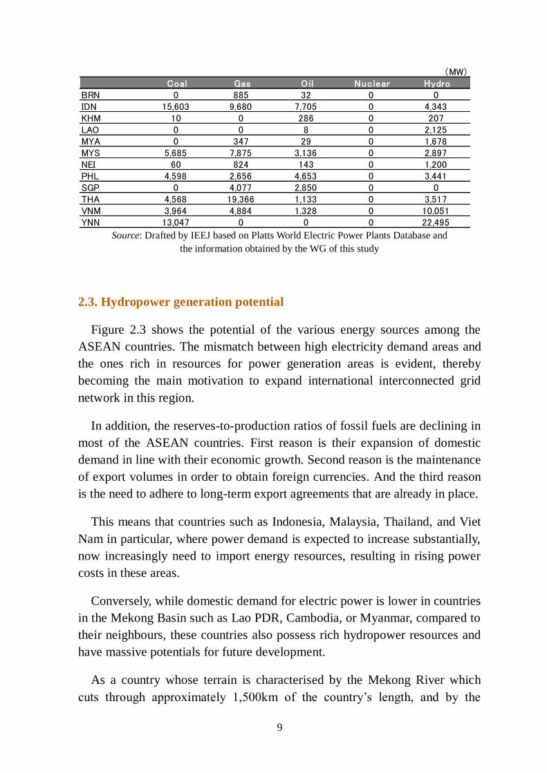
2.2. Projected power generation capacity

When assuming the power generation capacity for each country, the study

utilised the dataset published by Platts; “World Electric Power Plants

Database (as of 2012)”. This dataset was segregated by country, type and

installed capacity. For some countries, figures are based on information

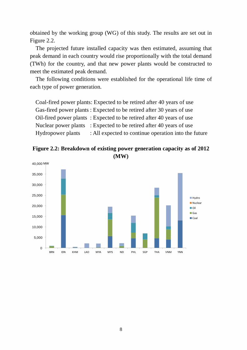
8

obtained by the working group (WG) of this study. The results are set out in

Figure 2.2.

The projected future installed capacity was then estimated, assuming that

peak demand in each country would rise proportionally with the total demand

(TWh) for the country, and that new power plants would be constructed to

meet the estimated peak demand.

The following conditions were established for the operational life time of

each type of power generation.

Coal-fired power plants: Expected to be retired after 40 years of use

Gas-fired power plants : Expected to be retired after 30 years of use

Oil-fired power plants : Expected to be retired after 40 years of use

Nuclear power plants : Expected to be retired after 40 years of use

Hydropower plants : All expected to continue operation into the future

Figure 2.2: Breakdown of existing power generation capacity as of 2012

(MW)

0

5,000

10,000

15,000

20,000

25,000

30,000

35,000

40,000

BRN IDN KHM LAO MYA MYS NEI PHL SGP THA VNM YNN

Hydro

Nuclear

Oil

Gas

Coal

MW

9

Source: Drafted by IEEJ based on Platts World Electric Power Plants Database and

the information obtained by the WG of this study

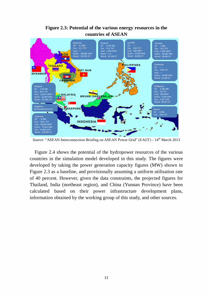
2.3. Hydropower generation potential

Figure 2.3 shows the potential of the various energy sources among the

ASEAN countries. The mismatch between high electricity demand areas and

the ones rich in resources for power generation areas is evident, thereby

becoming the main motivation to expand international interconnected grid

network in this region.

In addition, the reserves-to-production ratios of fossil fuels are declining in

most of the ASEAN countries. First reason is their expansion of domestic

demand in line with their economic growth. Second reason is the maintenance

of export volumes in order to obtain foreign currencies. And the third reason

is the need to adhere to long-term export agreements that are already in place.

This means that countries such as Indonesia, Malaysia, Thailand, and Viet

Nam in particular, where power demand is expected to increase substantially,

now increasingly need to import energy resources, resulting in rising power

costs in these areas.

Conversely, while domestic demand for electric power is lower in countries

in the Mekong Basin such as Lao PDR, Cambodia, or Myanmar, compared to

their neighbours, these countries also possess rich hydropower resources and

have massive potentials for future development.

As a country whose terrain is characterised by the Mekong River which

cuts through approximately 1,500km of the country’s length, and by the

（MW）Coal Gas Oil Nuclear Hydro

BRN 0 885 32 0 0IDN 15,603 9,680 7,705 0 4,343KHM 10 0 286 0 207LAO 0 0 8 0 2,125MYA 0 347 29 0 1,678MYS 5,685 7,875 3,136 0 2,897NEI 60 824 143 0 1,200PHL 4,598 2,656 4,653 0 3,441SGP 0 4,077 2,850 0 0THA 4,568 19,366 1,133 0 3,517VNM 3,964 4,884 1,328 0 10,051YNN 13,047 0 0 0 22,495

10

multiple tributary rivers which flow into the Mekong River from

high-elevation areas such as the Annamite Range, Lao PDR’s hydropower

development potential could theoretically be as high as 26,000 to 30,000MW.

It is estimated that no more than around one-tenth of this potential is currently

developed.

In addition, calculations by the Ministry of Industry, Mines, Energy

(MIME) of Cambodia estimate that the hydropower resources with

development potential in Cambodia could provide 10,000MW of power

(5,000MW from the main stream of the Mekong River itself, 4,000MW from

the subsidiary basin, and 1,000MW from other parts of the Mekong River);

and that no more than around 3 percent of this potential is currently

developed.

Furthermore, it is estimated that the hydropower potential of Myanmar

could theoretically reach 108,000MW, and development works making use of

economic cooperation and direct investment from China, Thailand and India

have gone into full swing in recent years.

Development of international grid networks in the EAS region is expected

to help optimise the power supply as a whole. In addition, power export

through interconnection becomes an important sector for economic growth in

these countries. Neighbouring countries will also benefit from the

diversification of their energy supplies and lower power costs through

importing power.

11

Figure 2.3: Potential of the various energy resources in the

countries of ASEAN

Source: “ASEAN Interconnection Briefing on ASEAN Power Grid” (EAGT) - 14th March 2013

Figure 2.4 shows the potential of the hydropower resources of the various

countries in the simulation model developed in this study. The figures were

developed by taking the power generation capacity figures (MW) shown in

Figure 2.3 as a baseline, and provisionally assuming a uniform utilisation rate

of 40 percent. However, given the data constraints, the projected figures for

Thailand, India (northeast region), and China (Yunnan Province) have been

calculated based on their power infrastructure development plans,

information obtained by the working group of this study, and other sources.

Lao PDR

Oil : －Gas : 3.60 TCFCoal : 600 MMTHydro : 26,500 MWWood : 46,006 KT

Cambodia

Oil : －Gas : 9.89 TCF

Coal : －Hydro : 10,000 MWWood : 81,565 KT

SingaporeNo Energy Resources

IndonesiaOil : 10 BBLGas : 169.5 TCFCoal : 38,000 MMTHydro : 75,625 MWGeo : 19,658 MWWood : 439,049 KT

PhilippinesOil : 0.285 BBLGas : 4.6 TCFCoal : 346 MMTHydro : 9,150 MWGeo : 2,047 MWWood : 89,267 KT

VietnamOil : 5 BBLGas : 19.2 TCFCoal : 4,500 MMTHydro : 68,500 MWWood : 48,960 KT

BruneiOil : 6 BBLGas : 34.8 TCF

MyanmarOil : 3.1 BBLGas : 12.1 TCF

Coal : －Hydro : 108,000 MWWood : 129,935 KT

MalaysiaOil : 3.42 BBLGas : 84.4 TCFCoal : 1,024.5 MMTHydro : 25,000 MWWood : 137,301 KT

ThailandOil : 0.156 BBLGas : 12.2 TCFCoal : 1,240 MMTHydro : n.d.Wood : 67,130 KT

12

Figure 2.4: Projected hydropower development potential in 2035 (TWh)

Source: IEEJ projections

2.4. Projected load curve

The development of power resources is dictated by the power demand

during peak times rather than by the annual power demand for the country in

question. In recent years, there have been changes in the load curve in much

of the East Asian region due to changes in the industrial structure and living

environments in the region.

As early as the mid-1990s, power consumption patterns in Thailand, the

Philippines, Indonesia (Java-Bali Transmission Line), and Viet Nam

(southern region) were beginning to display a load curve which peaked

during the daytime when industrial demand is high since these countries are

relatively mature markets.

Meanwhile, the power consumption patterns of other East Asian countries

have, until recent years, retained the traditional electric lighting-centered

demand mode, where the daily peak occurs from early evening through

nighttime. However, with the growing power demand for industrial purposes

in recent years due to economic development, there are now signs that the

rate of increase in the daytime peak is starting to exceed the rate of interest in

265.0

35.0

92.9

378.4

87.6 64.4

32.1 16.4

240.0

414.2

0

50

100

150

200

250

300

350

400

450

BRN IDN KHM LAO MYA MYS NEI PHL SGP THA VNM YNN

TWh

13

the nighttime peak. This means that the extent of the gap between the daytime

and nighttime peaks in power demand is decreasing year on year.

Although future long-term trends in the load curve are difficult to predict

with any accuracy because they are intricately connected with a range of

factors, including culture and climate, as well as the economic circumstances

of the country or region, the simulation model created by this report has been

established as follows.

As a general rule, peak power for each country was established using the

daily load curve and load duration curve on the days of maximum power

demand taken from the most recent data that could be obtained for each

country. However, for countries where such data were difficult to obtain, the

peak power was established using data from neighbouring countries where

the pace of economic development was similar.

The following figures show the daily load curve and load duration curve

projected for each country in the simulation model of this study. However,

given the data constraints, the projected curves for Yunnan province in China

have been assumed to be similar to Viet Nam’s data.

Figure 2.5: Daily load curve (average for 2006) and load duration curve

for BRN

Source: by IEEJ based on Japan Electric Power Information Center (JEPIC) materials

0

50

100

150

200

250

300

0 2 4 6 8 10 12 14 16 18 20 22

MW

TIME

0.0

0.2

0.4

0.6

0.8

1.0

1.2

0 200 400 600 800 1,000 1,200 1,400 1,600

INDEX (1.0=Maximum Demand)

MINUTES

14

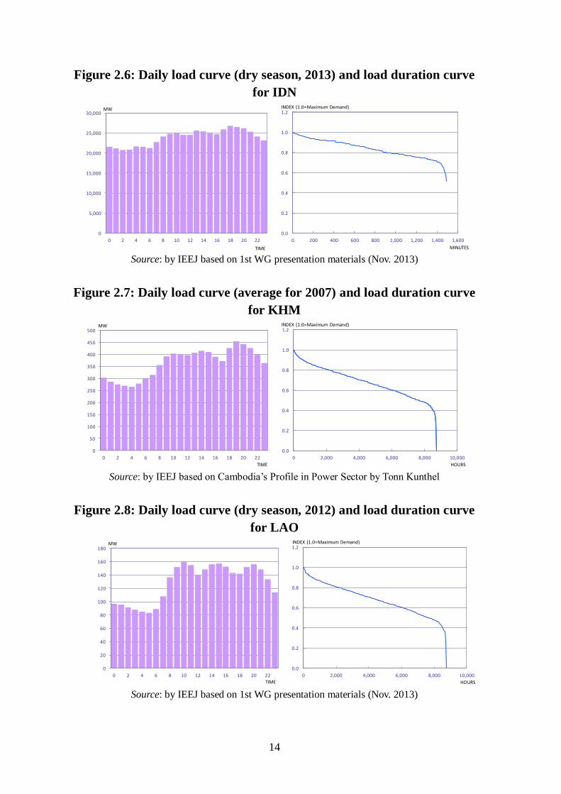
Figure 2.6: Daily load curve (dry season, 2013) and load duration curve

for IDN

Source: by IEEJ based on 1st WG presentation materials (Nov. 2013)

Figure 2.7: Daily load curve (average for 2007) and load duration curve

for KHM

Source: by IEEJ based on Cambodia’s Profile in Power Sector by Tonn Kunthel

Figure 2.8: Daily load curve (dry season, 2012) and load duration curve

for LAO

Source: by IEEJ based on 1st WG presentation materials (Nov. 2013)

0

5,000

10,000

15,000

20,000

25,000

30,000

0 2 4 6 8 10 12 14 16 18 20 22

MW

TIME

0.0

0.2

0.4

0.6

0.8

1.0

1.2

0 200 400 600 800 1,000 1,200 1,400 1,600

INDEX (1.0=Maximum Demand)

MINUTES

0

50

100

150

200

250

300

350

400

450

500

0 2 4 6 8 10 12 14 16 18 20 22

MW

TIME

0.0

0.2

0.4

0.6

0.8

1.0

1.2

0 2,000 4,000 6,000 8,000 10,000

INDEX (1.0=Maximum Demand)

HOURS

0

20

40

60

80

100

120

140

160

180

0 2 4 6 8 10 12 14 16 18 20 22

MW

TIME

0.0

0.2

0.4

0.6

0.8

1.0

1.2

0 2,000 4,000 6,000 8,000 10,000

INDEX (1.0=Maximum Demand)

HOURS

15

Figure 2.9: Daily load curve (rainy season, 2007) and load duration curve

for MYA

Source: by IEEJ based on JEPIC materials

Figure 2.10: Daily load curve (June 2012) and load duration curve for

MYS

Source: Energy Commission, Grid System Operation and Performance Report 1st Half 2012

Figure 2.11: Daily load curve (July 2013) and load duration curve for NEI

Source: by IEEJ based on 1st WG presentation materials (Nov. 2013)

0

200

400

600

800

1,000

1,200

1,400

0 2 4 6 8 10 12 14 16 18 20 22

MW

TIME

0.0

0.2

0.4

0.6

0.8

1.0

1.2

0 2,000 4,000 6,000 8,000 10,000

INDEX (1.0=Maximum Demand)

HOURS

0

2,000

4,000

6,000

8,000

10,000

12,000

14,000

16,000

18,000

0 2 4 6 8 10 12 14 16 18 20 22

MW

TIME

0.0

0.2

0.4

0.6

0.8

1.0

1.2

0 200 400 600 800 1,000 1,200 1,400 1,600

INDEX (1.0=Maximum Demand)

MINUTES

0

500

1,000

1,500

2,000

2,500

0 2 4 6 8 10 12 14 16 18 20 22

MW

TIME

0.0

0.2

0.4

0.6

0.8

1.0

1.2

0 2,000 4,000 6,000 8,000 10,000

INDEX (1.0=Maximum Demand)

HOURS

16

Figure 2.12: Daily load curve (September 2011) and load duration curve

for PHL

Source: Manila Electric Company (MERALCO), Investors’ Briefing & Teleconference 2011

Figure 2.13: Daily load curve (May 2010) and load duration curve for

SPG

Source: Energy Market Authority, Statement of Opportunities for the Singapore Energy Industry

2011

Figure 2.14: Daily load curve (April 2012) and load duration curve for

THA

Source: by IEEJ based on 1st WG presentation materials (Nov. 2013)

0

1,000

2,000

3,000

4,000

5,000

6,000

0 2 4 6 8 10 12 14 16 18 20 22

MW

TIME

0.0

0.2

0.4

0.6

0.8

1.0

1.2

0 2,000 4,000 6,000 8,000 10,000

HOURS

INDEX (1.0=Maximum Demand)

0

1,000

2,000

3,000

4,000

5,000

6,000

7,000

0 2 4 6 8 10 12 14 16 18 20 22

MW

TIME

0.0

0.2

0.4

0.6

0.8

1.0

1.2

0 200 400 600 800 1,000 1,200 1,400 1,600

INDEX (1.0=Maximum Demand)

MINUTES

0

5,000

10,000

15,000

20,000

25,000

30,000

0 2 4 6 8 10 12 14 16 18 20 22

MW

TIME

0.0

0.2

0.4

0.6

0.8

1.0

1.2

0 2,000 4,000 6,000 8,000 10,000

INDEX (1.0=Maximum Demand)

HOURS

17

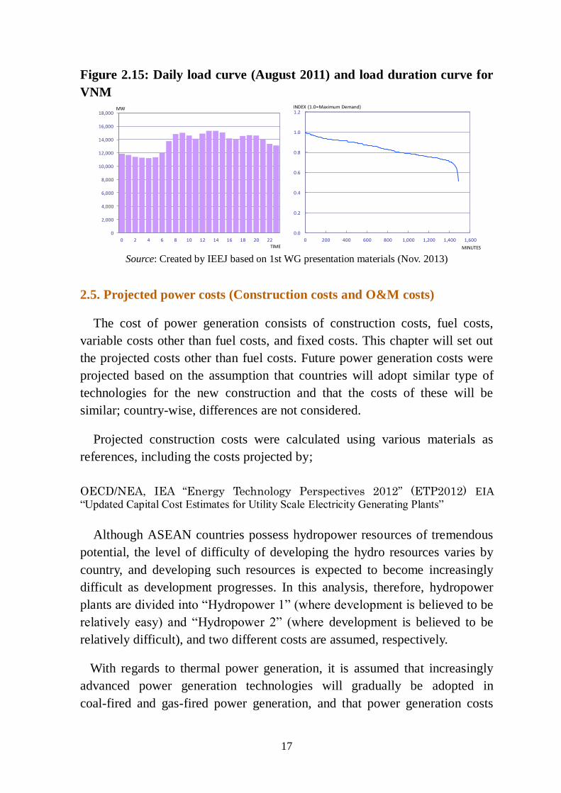
Figure 2.15: Daily load curve (August 2011) and load duration curve for

VNM

Source: Created by IEEJ based on 1st WG presentation materials (Nov. 2013)

2.5. Projected power costs (Construction costs and O&M costs)

The cost of power generation consists of construction costs, fuel costs,

variable costs other than fuel costs, and fixed costs. This chapter will set out

the projected costs other than fuel costs. Future power generation costs were

projected based on the assumption that countries will adopt similar type of

technologies for the new construction and that the costs of these will be

similar; country-wise, differences are not considered.

Projected construction costs were calculated using various materials as

references, including the costs projected by;

OECD/NEA, IEA “Energy Technology Perspectives 2012” (ETP2012) EIA

“Updated Capital Cost Estimates for Utility Scale Electricity Generating Plants”

Although ASEAN countries possess hydropower resources of tremendous

potential, the level of difficulty of developing the hydro resources varies by

country, and developing such resources is expected to become increasingly

difficult as development progresses. In this analysis, therefore, hydropower

plants are divided into “Hydropower 1” (where development is believed to be

relatively easy) and “Hydropower 2” (where development is believed to be

relatively difficult), and two different costs are assumed, respectively.

With regards to thermal power generation, it is assumed that increasingly

advanced power generation technologies will gradually be adopted in

coal-fired and gas-fired power generation, and that power generation costs

0

2,000

4,000

6,000

8,000

10,000

12,000

14,000

16,000

18,000

0 2 4 6 8 10 12 14 16 18 20 22

MW

TIME

0.0

0.2

0.4

0.6

0.8

1.0

1.2

0 200 400 600 800 1,000 1,200 1,400 1,600

INDEX (1.0=Maximum Demand)

MINUTES

18

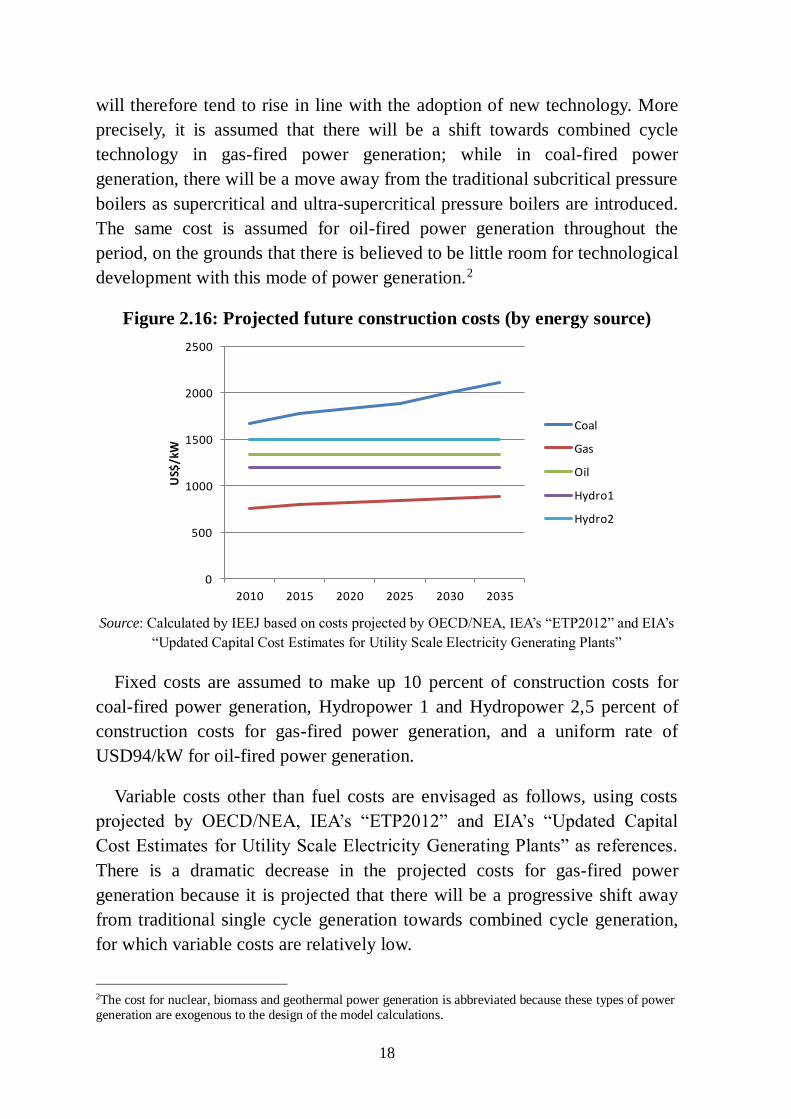
will therefore tend to rise in line with the adoption of new technology. More

precisely, it is assumed that there will be a shift towards combined cycle

technology in gas-fired power generation; while in coal-fired power

generation, there will be a move away from the traditional subcritical pressure

boilers as supercritical and ultra-supercritical pressure boilers are introduced.

The same cost is assumed for oil-fired power generation throughout the

period, on the grounds that there is believed to be little room for technological

development with this mode of power generation.2

Figure 2.16: Projected future construction costs (by energy source)

Source: Calculated by IEEJ based on costs projected by OECD/NEA, IEA’s “ETP2012” and EIA’s

“Updated Capital Cost Estimates for Utility Scale Electricity Generating Plants”

Fixed costs are assumed to make up 10 percent of construction costs for

coal-fired power generation, Hydropower 1 and Hydropower 2,5 percent of

construction costs for gas-fired power generation, and a uniform rate of

USD94/kW for oil-fired power generation.

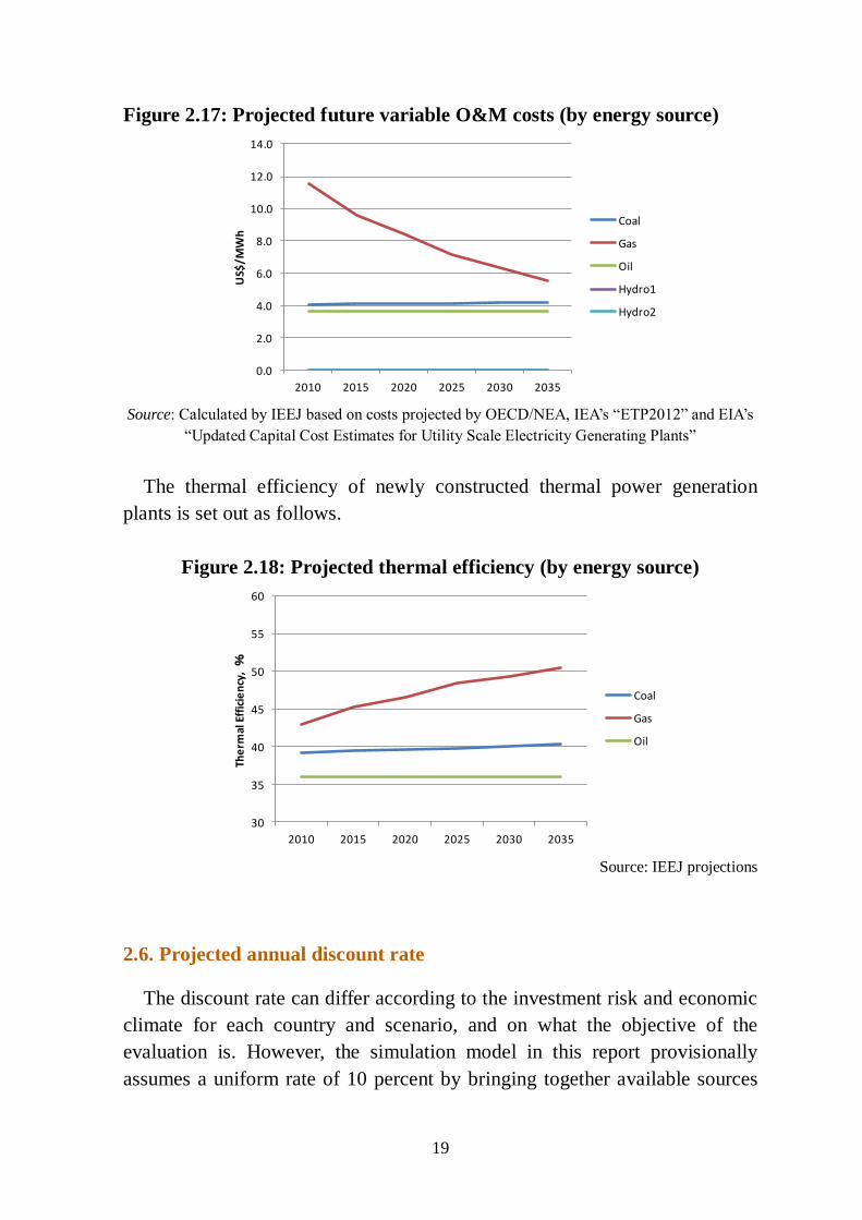
Variable costs other than fuel costs are envisaged as follows, using costs

projected by OECD/NEA, IEA’s “ETP2012” and EIA’s “Updated Capital

Cost Estimates for Utility Scale Electricity Generating Plants” as references.

There is a dramatic decrease in the projected costs for gas-fired power

generation because it is projected that there will be a progressive shift away

from traditional single cycle generation towards combined cycle generation,

for which variable costs are relatively low.

2The cost for nuclear, biomass and geothermal power generation is abbreviated because these types of power generation are exogenous to the design of the model calculations.

0

500

1000

1500

2000

2500

2010 2015 2020 2025 2030 2035

US$

/kW

Coal

Gas

Oil

Hydro1

Hydro2

19

Figure 2.17: Projected future variable O&M costs (by energy source)

Source: Calculated by IEEJ based on costs projected by OECD/NEA, IEA’s “ETP2012” and EIA’s

“Updated Capital Cost Estimates for Utility Scale Electricity Generating Plants”

The thermal efficiency of newly constructed thermal power generation

plants is set out as follows.

Figure 2.18: Projected thermal efficiency (by energy source)

Source: IEEJ projections

2.6. Projected annual discount rate

The discount rate can differ according to the investment risk and economic

climate for each country and scenario, and on what the objective of the

evaluation is. However, the simulation model in this report provisionally

assumes a uniform rate of 10 percent by bringing together available sources

0.0

2.0

4.0

6.0

8.0

10.0

12.0

14.0

2010 2015 2020 2025 2030 2035

US$

/MW

h

Coal

Gas

Oil

Hydro1

Hydro2

30

35

40

45

50

55

60

2010 2015 2020 2025 2030 2035

The

rmal

Eff

icie

ncy

, ％

Coal

Gas

Oil

20

of information and opinions from several experts.

2.7. Projected fuel costs

Future costs for coal and natural gas were projected as follows.

Projected coal prices were divided into two levels: prices for

coal-producing countries and prices for coal-importing countries. Indonesia,

Malaysia, the Philippines, Thailand, Viet Nam, Myanmar, Lao PDR,

Cambodia, China and India are coal-producing countries. Two other

countries—Singapore and Brunei—are coal-importing countries. Coal prices

for 2010 are set at USD60/ton for coal-producing countries and USD90/ton

for coal-importing countries. The price of USD60/ton for coal-producing

countries was determined based on the extraction costs plus costs of

transportation to ports. Prices are expected to rise by USD2.5/ton per year

from 2010 onwards, taking inflation and the rising costs of coal production

into consideration. This rate of increase was determined based on the

estimated average rate of increase in Asian costs, insurance, and freight (CIF)

calculated for the period between 1991 and 2013 in IEA Coal Information

2013.

Figure 2.19: Projected future coal prices (Steam coal)

Source: IEEJ projections

Projected prices for natural gas are divided into three levels: countries

which import natural gas and do not produce any domestically (Singapore

and the Philippines); countries which currently possess some domestic gas

fields but where the price of gas used domestically is relatively high

0.00

20.00

40.00

60.00

80.00

100.00

120.00

140.00

160.00

180.00

2010 2015 2020 2025 2030 2035

US$

/ton

ne

SGP, BRN

IDN, MYS, PHL, THA, VNM, MYA,

LAO, KHM, YNN, NEI

21

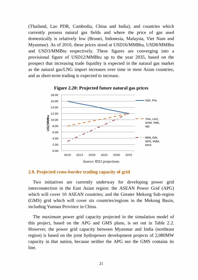
(Thailand, Lao PDR, Cambodia, China and India); and countries which

currently possess natural gas fields and where the price of gas used

domestically is relatively low (Brunei, Indonesia, Malaysia, Viet Nam and

Myanmar). As of 2010, these prices stood at USD16/MMBtu, USD8/MMBtu

and USD3/MMBtu respectively. These figures are converging into a

provisional figure of USD12/MMBtu up to the year 2035, based on the

prospect that increasing trade liquidity is expected in the natural gas market

as the natural gas/LNG import increases over time in most Asian countries,

and as short-term trading is expected to increase.

Figure 2.20: Projected future natural gas prices

Source: IEEJ projections

2.8. Projected cross-border trading capacity of grid

Two initiatives are currently underway for developing power grid

interconnection in the East Asian region: the ASEAN Power Grid (APG)

which will cover 10 ASEAN countries; and the Greater Mekong Sub-region

(GMS) grid which will cover six countries/regions in the Mekong Basin,

including Yunnan Province in China.

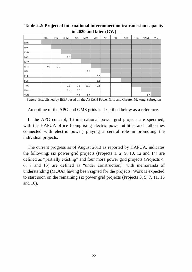
The maximum power grid capacity projected in the simulation model of

this project, based on the APG and GMS plans, is set out in Table 2.2.

However, the power grid capacity between Myanmar and India (northeast

region) is based on the joint hydropower development projects of 2,080MW

capacity in that nation, because neither the APG nor the GMS contains its

line.

0.00

2.00

4.00

6.00

8.00

10.00

12.00

14.00

16.00

18.00

2010 2015 2020 2025 2030 2035

US$

/MM

Btu

SGP, PHL

THA, LAO, KHM, YNN, NEI

BRN, IDN, MYS, VNM, MYA

22

Table 2.2: Projected international interconnection transmission capacity

in 2020 and later (GW)

Source: Established by IEEJ based on the ASEAN Power Grid and Greater Mekong Subregion

An outline of the APG and GMS grids is described below as a reference.

In the APG concept, 16 international power grid projects are specified,

with the HAPUA office (comprising electric power utilities and authorities

connected with electric power) playing a central role in promoting the

individual projects.

The current progress as of August 2013 as reported by HAPUA, indicates

the following: six power grid projects (Projects 1, 2, 9, 10, 12 and 14) are

defined as “partially existing” and four more power grid projects (Projects 4,

6, 8 and 13) are defined as “under construction,” with memoranda of

understanding (MOUs) having been signed for the projects. Work is expected

to start soon on the remaining six power grid projects (Projects 3, 5, 7, 11, 15

and 16).

BRN IDN KHM LAO MYA MYS NEI PHL SGP THA VNM YNN

BRN

IDN

KHM

LAO 0.3

MYA

MYS 0.3 2.2

NEI 2.1

PHL 0.5

SGP 1.1

THA 2.3 7.9 11.7 0.8

VNM 0.4 2.7

YNN 3.0 2.0 8.5

23

Figure 2.21: ASEAN Power Grid (APG)

Source: HAPUA Secretariat, “APG Interconnection Status”-Revised by August 2013

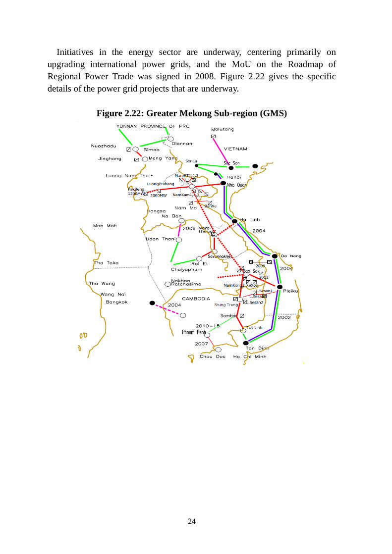
The GMS program is an inter-regional development program led by the

ADB in which multisectoral partnerships are being developed in the Mekong

Basin region in infrastructure domains, including transportation, energy and

communication, among six countries/regions consisting of Cambodia, Lao

PDR, Myanmar, Thailand, Viet Nam and China (Yunnan Province, with the

Guangxi Zhuang Autonomous Region also participating since 2004).

24

Initiatives in the energy sector are underway, centering primarily on

upgrading international power grids, and the MoU on the Roadmap of

Regional Power Trade was signed in 2008. Figure 2.22 gives the specific

details of the power grid projects that are underway.

Figure 2.22: Greater Mekong Sub-region (GMS)

25

Source: ADB, “Roadmap for Energy and Power Integration in the GMS” - 29th September 2009

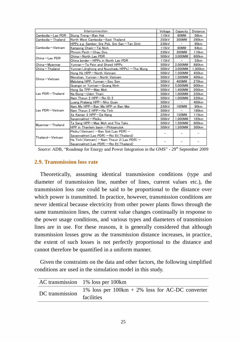
2.9. Transmission loss rate

Theoretically, assuming identical transmission conditions (type and

diameter of transmission line, number of lines, current values etc.), the

transmission loss rate could be said to be proportional to the distance over

which power is transmitted. In practice, however, transmission conditions are

never identical because electricity from other power plants flows through the

same transmission lines, the current value changes continually in response to

the power usage conditions, and various types and diameters of transmission

lines are in use. For these reasons, it is generally considered that although

transmission losses grow as the transmission distance increases, in practice,

the extent of such losses is not perfectly proportional to the distance and

cannot therefore be quantified in a uniform manner.

Given the constraints on the data and other factors, the following simplified

conditions are used in the simulation model in this study.

AC transmission 1% loss per 100km

DC transmission 1% loss per 100km + 2% loss for AC-DC converter

facilities

Voltage Capacity DistanceCambodia－Lao PDR Stung Treng－Ban Hat 115kV 80MW 56kmCambodia－Thailand North West Cambodia－East Thailand 250kV 300MW 290km

HPPs e.g. Sambor, Sre Pok, Sre San－Tan Dinh 230kV - 90kmKampong Cham－Tai Ninh 115kV 80MW 64kmPhnom Penh－Chau Doc 230kV 300MW 110kmChina－North Lao PDR 500kV 3,000MW 600kmChina border－HPPs in North Lao PDR 115kV - 33km

China－Myanmar Yunnan－Ta Pein and Shweli HPPs 500kV 2,000MW 880kmChina－Thailand Yunnan（Jinghong and Nuozhadu HPPs）－Tha Wung 500kV 3,000MW 1,300km

Hong He HPP－North Vietnam 500kV 1,500MW 450kmWenshan, Yunnan－North Vietnam 500kV 1,500MW 400kmMalutang HPP, Yunnan－Soc Son 500kV 460MW 270kmGuangxi or Yunnan－Quang Ninh 500kV 5,000MW 600kmHong Sa TPP－Mae Moh 500kV 1,400MW 200kmNa Bong－Udon Thani 500kV 1,000MW 220kmNam Theun 2 HPP－Roi Et 2 500kV 1,000MW 220kmLuang Prabang HPP－Nho Quan 500kV - 400kmNam Mo HPP－Ban Ma HPP or Ban Mai 230kV 100MW 90kmNam Theun 2 HPP－Ha Tinh 500kV - 190kmXe Kaman 3 HPP－Da Nang 220kV 150MW 115kmSavannakhet－Pleiku 500kV 1,000MW 165kmTa Sang HPP－Mae Moh and Tha Tako 500kV 1,500MW 600kmHPP in Thanlwin basin－Phitsanulok 500kV 1,500MW 300kmPleiku（Vietnam）－Ban Sok（Lao PDR）－Savannakhet（Lao PDR）－Roi Et（Thailand）

- - -

Ha Tinh（Vietnam）－Nam Theun 2（Lao PDR）－Savannakhet（Lao PDR）－Roi Et（Thailand）

- - -

Lao PDR－Vietnam

Myanmar－Thailand

Thailand－Vietnam

Interconnection

Cambodia－Vietnam

China－Lao PDR

China－Vietnam

Lao PDR－Thailand

26

2.10. Transmission costs

When calculating costs associated with power transmission, the actual

construction costs of the transmission plants and the costs of repairing,

maintaining and managing these facilities must be considered. In addition,

when constructing power grids within the East Asian region, the need for

submarine cables for supplying power to opposite sides of channels and to

islands must be taken into consideration, as well as the construction of the

usual overhead transmission lines.

The conditions for calculating such transmission costs in the simulation

model of this report are as follows.

Principally, the individual costs of all facilities including power lines,

pylons and transformer stations should be massed in order to estimate the

transmission line construction costs. However, given the data constraints, in

this simulation model, unit costs per unit of distance (km) are assumed for the

whole transmission lines excluding transformer stations, and the costs

calculated according to the transmission distance. By adding this figure to the

construction costs according to the number of transformer stations (switching

stations) that are likely to be needed for the route in question, an estimate is

obtained for the total costs required.

In a precise sense, the unit construction costs for the transmission line

stands at USD0.9 million/km/2 circuits for overhead lines and USD5

million/km/2 circuits for submarine cables, based on the most recent actual

performance figures for construction in neighbouring countries. The

estimated sum of construction costs of transformer stations (switching

stations) was obtained by assuming fixed costs3 of USD20 million per

station, and adding additional costs4 of USD10 million per line.

Turning to O&M costs, ideally, the personnel costs, raw material costs and

others should be estimated separately. However, given the data constraints,

total construction costs of approximately 0.3 percent/year were assumed in

this simulation model.

3Shared costs required to install a single switching station such as the cost of securing land and installing

shared facilities. 4Costs required for installing the number of devices in accordance with the number of lines.

27

CHAPTER 3

OPTIMISING POWER INFRASTRUCTURE DEVELOPMENT

Optimising calculations were carried out according to the conditions set in

the previous chapter, using an optimal power generation planning model and

a supply reliability evaluation model employing the Monte Carlo method. An

overview is displayed below.

3.1. Model overview

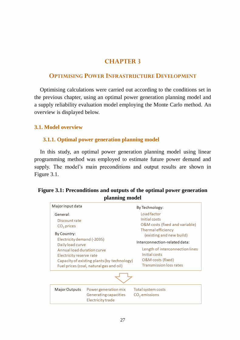
3.1.1. Optimal power generation planning model

In this study, an optimal power generation planning model using linear

programming method was employed to estimate future power demand and

supply. The model’s main preconditions and output results are shown in

Figure 3.1.

Figure 3.1: Preconditions and outputs of the optimal power generation

planning model

28

In this model, the cost-optimal (i.e. the minimum total system cost) power

generation mix for each country is estimated, with preconditions such as the

power demand and load curve of each country and the cost and efficiency of

each power generating technology.

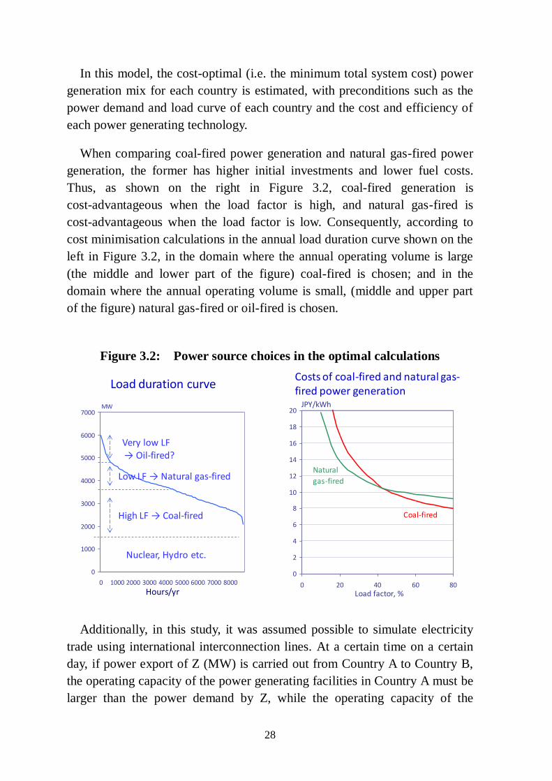
When comparing coal-fired power generation and natural gas-fired power

generation, the former has higher initial investments and lower fuel costs.

Thus, as shown on the right in Figure 3.2, coal-fired generation is

cost-advantageous when the load factor is high, and natural gas-fired is

cost-advantageous when the load factor is low. Consequently, according to

cost minimisation calculations in the annual load duration curve shown on the

left in Figure 3.2, in the domain where the annual operating volume is large

(the middle and lower part of the figure) coal-fired is chosen; and in the

domain where the annual operating volume is small, (middle and upper part

of the figure) natural gas-fired or oil-fired is chosen.

Figure 3.2: Power source choices in the optimal calculations

Additionally, in this study, it was assumed possible to simulate electricity

trade using international interconnection lines. At a certain time on a certain

day, if power export of Z (MW) is carried out from Country A to Country B,

the operating capacity of the power generating facilities in Country A must be

larger than the power demand by Z, while the operating capacity of the

0

1000

2000

3000

4000

5000

6000

7000

0 1000 2000 3000 4000 5000 6000 7000 8000

MW

Nuclear, Hydro etc.

Load duration curve

High LF → Coal-fired

Low LF → Natural gas-fired

Very low LF → Oil-fired?

0

2

4

6

8

10

12

14

16

18

20

0 20 40 60 80

JPY/kWh

Coal-fired

Natural

gas-fired

Load factor, %Hours/yr

Costs of coal-fired and natural gas-fired power generation

29

facilities in Country B will be less than the demand by Z × (1 - transmission

loss rate). Here, Z cannot exceed the transmission line capacity, and alongside

the cost incurred in constructing transmission lines, if an upper limit is set on

the transmission line capacity, Z cannot exceed that upper limit.

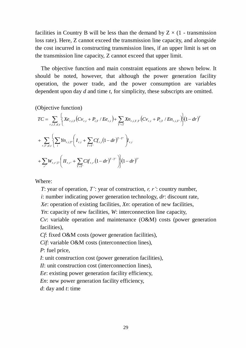
The objective function and main constraint equations are shown below. It

should be noted, however, that although the power generation facility

operation, the power trade, and the power consumption are variables

dependent upon day d and time t, for simplicity, these subscripts are omitted.

(Objective function)

Where:

T: year of operation, T’: year of construction, r, r’: country number,

i: number indicating power generation technology, dr: discount rate,

Xe: operation of existing facilities, Xn: operation of new facilities,

Yn: capacity of new facilities, W: interconnection line capacity,

Cv: variable operation and maintenance (O&M) costs (power generation

facilities),

Cf: fixed O&M costs (power generation facilities),

Cif: variable O&M costs (interconnection lines),

P: fuel price,

I: unit construction cost (power generation facilities),

II: unit construction cost (interconnection lines),

Ee: existing power generation facility efficiency,

En: new power generation facility efficiency,

d: day and t: time

TtdTir TT

TirTiirTTirirTiirTir drEnPCvXnEePCvXeTC

1//,,,, '

',,,,',,,,,,,,

tdTr

ir

TT

TT

irir

i

Tir IdrCfIYn,,',

,

'

'

,,',, 1

'

' '

'

',',',', 11T

r TT

TT

rrrrTrr drdrCifIIW

30

(Power supply and demand) For all d and t,

where D: power consumption (including transmission loss etc.), ir: auxiliary

power ratio,

Z: power trade: lr: transmission loss rate

(Existing facility power generation capacity constraints) For all d and t,

where Ye: existing facility capacity, F: load factor

(New facility power generation capacity constraints) For all d and t,

(Power trade capacity constraints) For all d and t,

(Supply reserve margin)

where PD: maximum demand, s: supply reserve rate

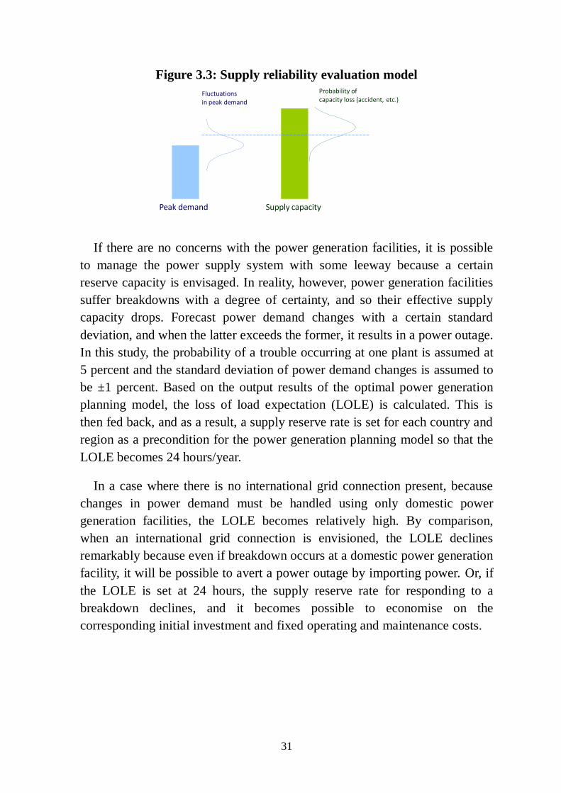
3.1.2. Supply reliability evaluation model

In these calculations, a supply reliability evaluation model employing the

Monte Carlo method was used in combination with the abovementioned

optimal power generation planning model. A conceptual diagram of this

model is shown in Figure 3.3.

'

,',,,'',

'

',,,,,, 11r

TrrTrrrri

i T

TTirTirTr ZZlrirXnXeD

i TT

TirTirirrTr YnYeFsPD'

',,,,,, 1

TirirTir YeFXe ,,,,,

TT

TrrTrr WZ'

',',,',

TT

TirirTir YnFXn'

',,,,,

31

Figure 3.3: Supply reliability evaluation model

If there are no concerns with the power generation facilities, it is possible

to manage the power supply system with some leeway because a certain

reserve capacity is envisaged. In reality, however, power generation facilities

suffer breakdowns with a degree of certainty, and so their effective supply

capacity drops. Forecast power demand changes with a certain standard

deviation, and when the latter exceeds the former, it results in a power outage.

In this study, the probability of a trouble occurring at one plant is assumed at

5 percent and the standard deviation of power demand changes is assumed to

be ±1 percent. Based on the output results of the optimal power generation

planning model, the loss of load expectation (LOLE) is calculated. This is

then fed back, and as a result, a supply reserve rate is set for each country and

region as a precondition for the power generation planning model so that the

LOLE becomes 24 hours/year.

In a case where there is no international grid connection present, because

changes in power demand must be handled using only domestic power

generation facilities, the LOLE becomes relatively high. By comparison,

when an international grid connection is envisioned, the LOLE declines

remarkably because even if breakdown occurs at a domestic power generation

facility, it will be possible to avert a power outage by importing power. Or, if

the LOLE is set at 24 hours, the supply reserve rate for responding to a

breakdown declines, and it becomes possible to economise on the

corresponding initial investment and fixed operating and maintenance costs.

Peak demand

Fluctuationsin peak demand

Supply capacity

Probability of capacity loss (accident, etc.)

32

3.2. Major assumptions and case settings

3.2.1. Major assumptions

In this study, the optimal power generation planning model and the supply

reliability evaluation model mentioned earlier were utilised to estimate the

optimum power generation mix and power trade up to 2035 by making use of

the data described in Chapter 2. Because the introduction of renewable energy

(other than hydro) and nuclear power are chiefly swayed by policy, they were

set in line with the forecast figures in the ERIA Outlook, and only thermal

power generation (coal, natural gas and oil) and hydropower generation were

calculated by the model. Of those energies, the introduction of hydropower

generation was as in the ERIA Outlook in Cases 0a, 0b and 1 discussed in the

following section, while in the other cases, the figures discussed in Chapter 2

were utilised to show additional hydro-potential.

In employing the optimal power generation planning model, the time

interval was assumed at five years. That is to say, 2010 is the latest actual

value, and the figures from 2015 onward are forecast figures. In the supply

reliability evaluation model, the number of trials with the Monte Carlo

method was approximately 140,000 times.

3.2.2. Case settings

The calculation cases were set as follows:

(1) Calculations covering the total system

Calculations were made based on the following case configurations, covering

all the 12 countries and regions:

Case 0 : Reference case (no additional grid connection)

Case 1 : Additional grid connection, no additional hydro-potential

Case 2a : Additional grid connection, additional hydro-potential

Case 2b : Additional grid connection, additional hydro-potential for export

purpose only

Case 3 : Same as Case 2b, with no upper limit set on the grid connection

capacity

Case 0 does not take grid connection into account, and is a scenario in

33

which a power generation mix is attained that resembles the ERIA Outlook

through the utilisation of the domestic power generation facilities of each

country only. Figure 3.4 presents a comparison between results of each

country’s 2035 mix (model output for Case 0) and the ERIA Outlook.

Figure 3.4: Comparison between the calculation results for each

country’s power generation mix and the ERIA Outlook

Generally, with low discount rates (for example, 3-5%), coal-fired power

generation is more cost-advantageous than natural gas-fired. In this study,

however, a relatively high real discount rate (10%) is envisioned, and so

selections are made with a certain ratio of both coal-fired and natural

gas-fired, according to each country’s load curve and load duration curve. For

the most part, those results do not show significant variance with ERIA’s

forecasts, but they do differ on several points.

First, in ERIA’s forecasts, oil-fired power generation is utilised in countries

such as Singapore and Indonesia, but in the results for the optimal model,

oil-fired is not selected due to its high cost. Conceivably, oil-fired would

actually be utilised based on contributing factors other than just cost such as

supply capability. That said, even in ERIA’s forecasts, the share accounted by

oil-fired is not high, and consequently in this study, no adjustment was made

to the model.

Second, in the ERIA Outlook, coal-fired is not utilised in Singapore or

Brunei. This is conceivable based on realistic supply capability. In this study,

an upper limit of zero was set for coal-fired in both of these countries.

Third, in ERIA’s forecasts, Thailand’s coal-fired ratio in 2035 is 15 percent,

which is relatively low. This is because in Thailand, until now, abundant

0%

10%

20%

30%

40%

50%

60%

70%

80%

90%

100%

mo

de

l

ERIA

mo

de

l

ERIA

mo

de

l

ERIA

mo

de

l

ERIA

mo

de

l

ERIA

mo

de

l

ERIA

mo

de

l

ERIA

mo

de

l

ERIA

mo

de

l

ERIA

mo

de

l

ERIA

mo

de

l

mo

de

l

sgp brn idn mys phl tha vnm mya lao khm ynn nei

Other renewables

Nuclear & geothermal

Hydro

Gas-fired

Oil-fired

Coal-fired

34

natural gas resources are being utilised. The construction of new coal-fired

power generation plants, however, is currently restricted mainly for political

reasons. Consequently, in this study, the 2035 coal-fired power generation

capacity was set at the same level as that of the ERIA Outlook by imposing

an upper limit constraint on new coal-fired power plant construction in

Thailand.

In the case of other countries, the model results are also made to basically

match ERIA’s forecasts by placing upper limit constraints on new facility

construction for either coal-fired or natural gas-fired. The reason why upper

limits were set here but not lower limits was in order to make it possible to

estimate how much the power generation capacity of coal- and natural

gas-fired, respectively, would decline according to the model, in the event

that supply from hydropower generation increases and supply from thermal

power decreases in Cases 2a, 2b and 3.

Case 1 was configured so that interconnection up to the upper limit set on

the grid connection capacity indicated in Table 2.2 is possible, but the

additional hydro-potential is not taken into account. In this case, as a result of

interconnection, the supply reserve margin is trimmed down, and the thermal

power-generation mix (the ratio of coal-fired and natural gas-fired) changes

slightly.

In Case 2a, as in Case 1, grid connection is made possible and additional

hydropower generation is possible with the hydropower generation potential

presented in Chapter 2 as the upper limit. In this case, as will be explained

later, additional hydropower generation is made to satisfy the domestic power

demands of the country concerned. In reality, in Indonesia, for example, due

to its characteristic features as an archipelago country, the domestic power

system itself is not connected as one. Thus, even if significant hydropower

generation potential existed in some islands, unless additional grid connection

was carried out, it would not be possible to fully utilise that potential. Similar

circumstances are present in other countries to some degree and consequently,

the ERIA Outlook does not assume that it will be possible to fully exploit

hydropower generation potential in order to meet domestic demand at least

over the period up to 2035. In this perspective, Case 2b was configured as a

case in which additional power generation can only be used for export and

cannot be exploited as supply to cover domestic demand.

35

Case 3 is similar to Case 2B, in which additional hydropower generation

can only be allocated to exports, but no cap is set on grid connection

capacities. Consequently, hydropower generation potential can be utilised

fully, and in particular, large amounts of power are exported from Myanmar,

which is envisioned to have the largest potential. Again, this is not necessarily

realistic, and Case 3 could be described as assessing what kind of situation

lies ahead should interconnection on a scale exceeding HAPUA’s upper limits

on interconnection becomes possible.

(2) Calculations covering specific interconnection lines

In addition to the calculations applicable to the total system as mentioned

above, in order to make it possible to assess the economics of the individual

interconnection lines discussed in Chapter 4, calculations were made for

cases that permitted grid connections between specific regions only, and were

compared against the case without grid connections. The assumed

connections are as follows:

a. Cambodia – Thailand (2.3GW)

b. Lao PDR – Thailand (7.9GW)

c. Myanmar – Thailand (11.7GW)

d. Myanmar – Thailand – Malaysia – Singapore (11.7GW/0.8GW/1.1GW)

e. Viet Nam – Lao PDR – Thailand (2.7GW/7.9GW)

f. Indonesia – Malaysia (2.2GW)

g. Lao PDR – Thailand – Malaysia – Singapore (7.9GW/0.8GW/1.1GW)

3.3. Results and discussions

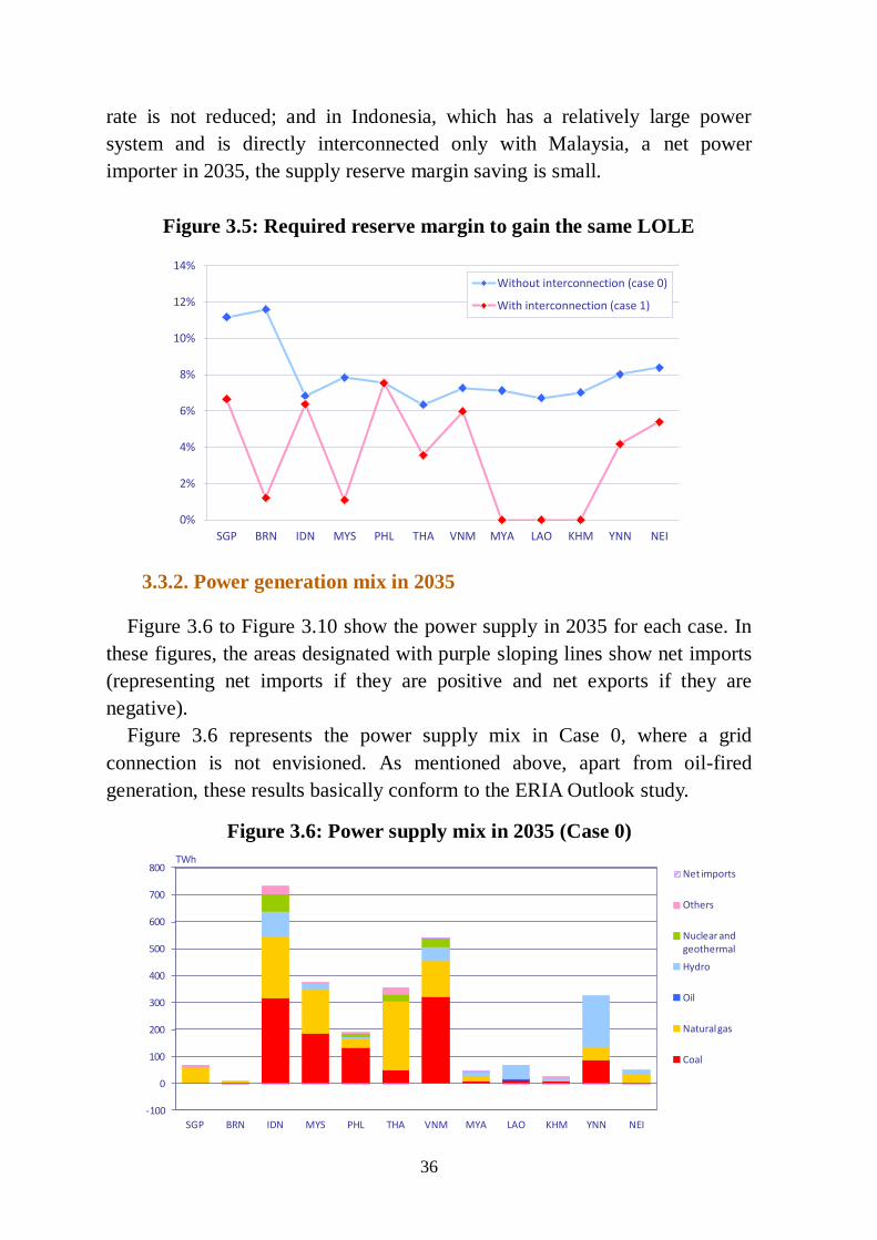
3.3.1. Supply reserve margin savings arising from grid connections

Figure 3.5 shows the supply reserve margin in each country and region. In

Case 0, which does not envisage a grid connection, the reserve margin is 7-8

percent for most countries, and around 11-12 percent for Singapore and

Brunei where the systems are small relative to the scale of the power

generation facilities. In the cases where grid connections are assumed, the

supply reserve margin to achieve the same 24-hour LOLE declines

substantially. The degree by which the reserve margin declines differs,

however, depending on the country. In the Philippines, where interconnection

does not take place due to the high interconnection costs, the supply reserve

36

-100

0

100

200

300

400

500

600

700

800

SGP BRN IDN MYS PHL THA VNM MYA LAO KHM YNN NEI

Net imports

Others

Nuclear and geothermal

Hydro

Oil

Natural gas

Coal

TWh

rate is not reduced; and in Indonesia, which has a relatively large power

system and is directly interconnected only with Malaysia, a net power

importer in 2035, the supply reserve margin saving is small.

Figure 3.5: Required reserve margin to gain the same LOLE

3.3.2. Power generation mix in 2035

Figure 3.6 to Figure 3.10 show the power supply in 2035 for each case. In

these figures, the areas designated with purple sloping lines show net imports

(representing net imports if they are positive and net exports if they are

negative).

Figure 3.6 represents the power supply mix in Case 0, where a grid

connection is not envisioned. As mentioned above, apart from oil-fired

generation, these results basically conform to the ERIA Outlook study.

Figure 3.6: Power supply mix in 2035 (Case 0)

0%

2%

4%

6%

8%

10%

12%

14%

SGP BRN IDN MYS PHL THA VNM MYA LAO KHM YNN NEI

Without interconnection (case 0)

With interconnection (case 1)

37

Figure 3.7 shows the power supply mix in Case 1. For this case,

hydropower generation is the same as for Case 0, but changes can be detected

in the thermal power generation. In Thailand the natural gas ratio is high in

Case 0 compared to the cost-optimised. Its natural gas-fired power generation

is reduced in Case 1 and is covered by coal-fired power generation from

neighbouring countries (in this instance Lao PDR). In this way, there is a

possibility that a more cost-optimal power generation mix could be achieved

through the utilisation of international interconnection lines, taking into

account each country’s particular restraints (in this case, restraints on new

coal-fired power plant construction in Thailand).

Figure 3.7: Power supply mix in 2035 (Case 1)

Figure 3.8 shows the power supply mix in Case 2a. In this case, utilisation

of additional hydropower potential in each country takes place and exports

occur from countries and areas possessing significant potential such as

Myanmar, Lao PDR, Cambodia, southern China and Northeast India to

Thailand, Viet Nam, Singapore and Brunei.

Additional hydropower generation potential also exists in countries such as

Indonesia, the Philippines and Viet Nam. In Case 2a, growth in hydropower

generation in these countries will be utilised to meet their domestic power

demands. Consequently, hydropower generation accounts for 36 percent of

total electricity supply in Indonesia and 45 percent in Viet Nam in 2035. In

reality, despite the hydropower generation potential that physically exists in

these countries, most of these resources cannot be utilised due to geographical

and economic factors. In view of this and as shown in the ERIA Outlook, a

-100

0

100

200

300

400

500

600

700

800

SGP BRN IDN MYS PHL THA VNM MYA LAO KHM YNN NEI

Net imports

Others

Nuclear and geothermal

Hydro

Oil

Natural gas

Coal

TWh

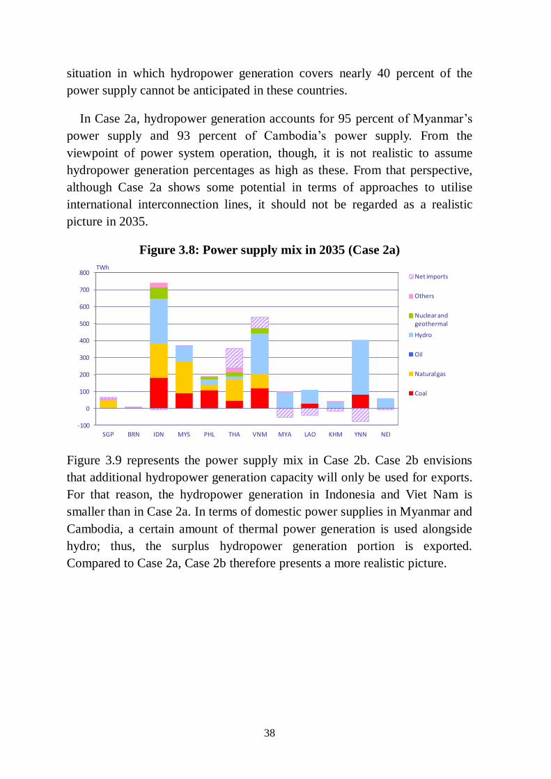
38

situation in which hydropower generation covers nearly 40 percent of the

power supply cannot be anticipated in these countries.

In Case 2a, hydropower generation accounts for 95 percent of Myanmar’s

power supply and 93 percent of Cambodia’s power supply. From the

viewpoint of power system operation, though, it is not realistic to assume

hydropower generation percentages as high as these. From that perspective,

although Case 2a shows some potential in terms of approaches to utilise

international interconnection lines, it should not be regarded as a realistic

picture in 2035.

Figure 3.8: Power supply mix in 2035 (Case 2a)

Figure 3.9 represents the power supply mix in Case 2b. Case 2b envisions

that additional hydropower generation capacity will only be used for exports.

For that reason, the hydropower generation in Indonesia and Viet Nam is

smaller than in Case 2a. In terms of domestic power supplies in Myanmar and

Cambodia, a certain amount of thermal power generation is used alongside

hydro; thus, the surplus hydropower generation portion is exported.

Compared to Case 2a, Case 2b therefore presents a more realistic picture.

-100

0

100

200

300

400

500

600

700

800

SGP BRN IDN MYS PHL THA VNM MYA LAO KHM YNN NEI

Net imports

Others

Nuclear and geothermal

Hydro

Oil

Natural gas

Coal

TWh

39

-100

0

100

200

300

400

500

600

700

800

SGP BRN IDN MYS PHL THA VNM MYA LAO KHM YNN NEI

Net imports

Others

Nuclear and geothermal

Hydro

Oil

Natural gas

Coal

TWh

Figure 3.9: Power supply mix in 2035 (Case 2b)

Figure 3.10 represents the power supply mix in Case 3. In this case,

hydropower generation in Myanmar in particular is extremely large, with the

country exporting 250TWh of electricity per year. At the same time, power is

also exported from Lao PDR, Cambodia, southern China and Northeast India

which contributes to the supply in Thailand, Viet Nam, Malaysia, Indonesia,

Singapore and Brunei. In reality, even if there were no upper limit constraints

on interconnection lines, the issue is whether or not the hydropower

generation potential in Myanmar could be economically developed on this

scale. This will therefore need to be studied further.

Figure 3.10: Power supply mix in 2035 (Case 3)

-300

-200

-100

0

100

200

300

400

500

600

700

800

SGP BRN IDN MYS PHL THA VNM MYA LAO KHM YNN NEI

Net imports

Others

Nuclear and geothermal

Hydro

Oil

Natural gas

Coal

TWh

40

Figure 3.11 shows the power supply mix for all 12 countries and regions

combined.

The area’s total power generation capacity will expand from 940TWh in

2010 to roughly 2,800TWh in 2035. In Case 0, which does not envisage grid

connection, the power generation mix in 2035 consists of coal-fired (40%),

natural gas-fired (36%), hydro (16%), and others such as nuclear and

renewables (7%). By comparison, in Case 1, the coal-fired thermal ratio

increases slightly to 41 percent.

In Case 2a, as a result of utilising additional hydropower generation

potential, the hydropower generation ratio rises to 44 percent and accordingly,

the shares covered by both coal-fired and natural gas-fired decline. By

comparison, in the more realistic scenario of Case 2b, the hydropower

generation ratio rises to 23 percent and in Case 3, which does not take grid

connection constraints into account, the ratio rises to 31 percent. In Cases 2b

and 3, the hydropower generation increases compared to Case 1; thus, the

dominance of natural gas-fired power generation declines accordingly.

Figure 3.11: Power supply mix by case in 2035 (total of the regions)

3.3.3. CO2 emissions in 2035

Figure 3.12 shows CO2 emissions in 2035 (the total for the 12 countries

and regions). Compared to Case 0, Case 1 does not have additional

hydropower generation and at the same time, the ratio of coal-fired power

0

500

1,000

1,500

2,000

2,500

3,000

Case 0 Case 1 Case 2a Case 2b Case 3

2010 2035

Others

Nuclear & geothermal

Hydro

Natural gas

Oil

Coal

TWh

41

generation increases slightly as a result of cost optimisation across the entire

system based on grid connection. ,. In view of this, CO2 emissions increase by

a small amount, from 1.346Gt in Case 0 to 1.354Gt in Case 1. By comparison,

in Cases 2a, 2b and 3, which make use of grid connection along with

additional hydropower generation, there are striking declines in CO2

emissions. This is especially true in Case 2a where the utilisation of domestic

hydro-potential in Indonesia and Viet Nam progresses, reducing CO2

emissions significantly to 0.85Gt. However, as mentioned above, this cannot

be described as a realistic case, The CO2 emission reductions compared to

Case 0 are around 0.07Gt in Case 2b, where a grid connection limit

corresponding to HAPUA’s limit is set; and around 0.15Gt in Case 3, which

does not set a limit to interconnection capacity.

Figure 3.12: CO2 emissions in 2035

3.3.4. Power trade flows in 2035

Figure 3.13 to Figure 3.16 show power trade flows in 2035.

In Case 1, which is shown in Figure 3.13, the quantity of power trade is

small compared to Cases 2a, 2b and 3 because the utilisation of additional

hydro-potential is not envisioned. However, even in this case, due to the

changes (in thermal power generation) power trade takes place with Thailand

being the biggest importer of power, followed by Singapore. The biggest

power exporter is Lao PDR, which supplies electricity to Thailand.

0.0

0.2

0.4

0.6

0.8

1.0

1.2

1.4

1.6

Case 0 Case 1 Case 2a Case 2b Case 3

GtCO2

1.35 1.35

0.85

1.271.20

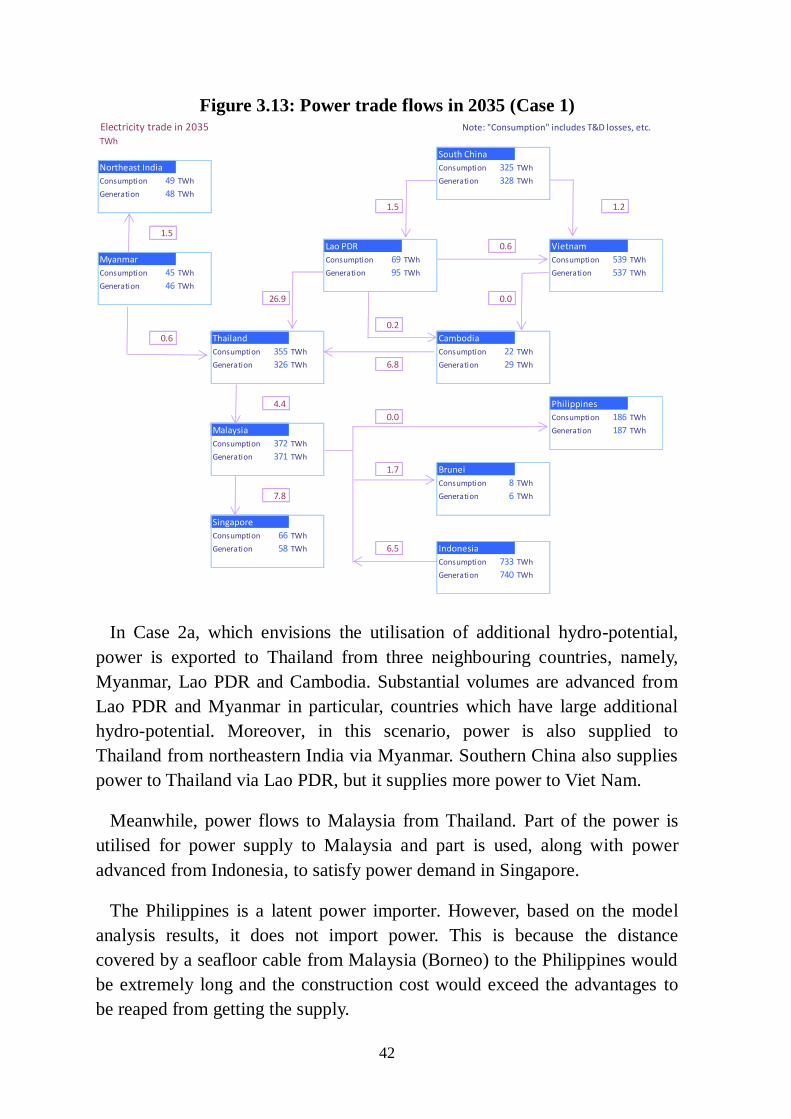
42

Figure 3.13: Power trade flows in 2035 (Case 1)

In Case 2a, which envisions the utilisation of additional hydro-potential,

power is exported to Thailand from three neighbouring countries, namely,

Myanmar, Lao PDR and Cambodia. Substantial volumes are advanced from

Lao PDR and Myanmar in particular, countries which have large additional

hydro-potential. Moreover, in this scenario, power is also supplied to

Thailand from northeastern India via Myanmar. Southern China also supplies

power to Thailand via Lao PDR, but it supplies more power to Viet Nam.

Meanwhile, power flows to Malaysia from Thailand. Part of the power is

utilised for power supply to Malaysia and part is used, along with power

advanced from Indonesia, to satisfy power demand in Singapore.

The Philippines is a latent power importer. However, based on the model

analysis results, it does not import power. This is because the distance

covered by a seafloor cable from Malaysia (Borneo) to the Philippines would

be extremely long and the construction cost would exceed the advantages to

be reaped from getting the supply.

Electricity trade in 2035 Note: "Consumption" includes T&D losses, etc.

TWh

South China

Northeast India Consumption 325 TWh

Consumption 49 TWh Generation 328 TWh

Generation 48 TWh

1.5 1.2

1.5

Lao PDR 0.6 Vietnam

Myanmar Consumption 69 TWh Consumption 539 TWh

Consumption 45 TWh Generation 95 TWh Generation 537 TWh

Generation 46 TWh

26.9 0.0

0.2

0.6 Thailand Cambodia

Consumption 355 TWh Consumption 22 TWh

Generation 326 TWh 6.8 Generation 29 TWh

4.4 Philippines

0.0 Consumption 186 TWh

Malaysia Generation 187 TWh

Consumption 372 TWh

Generation 371 TWh

1.7 Brunei

Consumption 8 TWh

7.8 Generation 6 TWh

Singapore

Consumption 66 TWh

Generation 58 TWh 6.5 Indonesia

Consumption 733 TWh

Generation 740 TWh

43

Figure 3.14: Power trade flows in 2035 (Case 2a)

Case 2b envisions a scenario in which additional hydropower generation

potential is not used to satisfy domestic demand in the country concerned but

only used for exporting. As mentioned above, this case is more realistic. From

the standpoint of the quantity of power trade, the outcomes in this case

basically resemble those in Case 2a.

Electricity trade in 2035 Note: "Consumption" includes T&D losses, etc.

TWh

South China

Northeast India Consumption 325 TWh

Consumption 49 TWh Generation 401 TWh

Generation 57 TWh

11.1 60.1

7.5

Lao PDR 4.9 Vietnam

Myanmar Consumption 69 TWh Consumption 539 TWh

Consumption 45 TWh Generation 110 TWh Generation 473 TWh

Generation 100 TWh

46.6 2.8

0.1

65.9 Thailand Cambodia

Consumption 355 TWh Consumption 22 TWh

Generation 240 TWh 12.9 Generation 38 TWh

5.0 Philippines

0.0 Consumption 186 TWh

Malaysia Generation 187 TWh

Consumption 372 TWh

Generation 368 TWh

1.7 Brunei

Consumption 8 TWh

7.8 Generation 6 TWh

Singapore

Consumption 66 TWh

Generation 58 TWh 8.8 Indonesia

Consumption 733 TWh

Generation 742 TWh

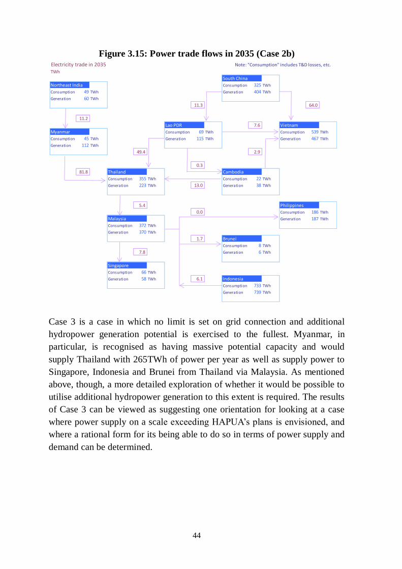
44

Figure 3.15: Power trade flows in 2035 (Case 2b)

Case 3 is a case in which no limit is set on grid connection and additional

hydropower generation potential is exercised to the fullest. Myanmar, in

particular, is recognised as having massive potential capacity and would

supply Thailand with 265TWh of power per year as well as supply power to

Singapore, Indonesia and Brunei from Thailand via Malaysia. As mentioned

above, though, a more detailed exploration of whether it would be possible to

utilise additional hydropower generation to this extent is required. The results

of Case 3 can be viewed as suggesting one orientation for looking at a case

where power supply on a scale exceeding HAPUA’s plans is envisioned, and

where a rational form for its being able to do so in terms of power supply and

demand can be determined.

Electricity trade in 2035 Note: "Consumption" includes T&D losses, etc.

TWh

South China

Northeast India Consumption 325 TWh

Consumption 49 TWh Generation 404 TWh

Generation 60 TWh

11.3 64.0

11.2

Lao PDR 7.6 Vietnam

Myanmar Consumption 69 TWh Consumption 539 TWh

Consumption 45 TWh Generation 115 TWh Generation 467 TWh

Generation 112 TWh

49.4 2.9

0.3

81.8 Thailand Cambodia

Consumption 355 TWh Consumption 22 TWh

Generation 223 TWh 13.0 Generation 38 TWh

5.4 Philippines

0.0 Consumption 186 TWh

Malaysia Generation 187 TWh

Consumption 372 TWh

Generation 370 TWh

1.7 Brunei

Consumption 8 TWh

7.8 Generation 6 TWh

Singapore

Consumption 66 TWh

Generation 58 TWh 6.1 Indonesia

Consumption 733 TWh

Generation 739 TWh

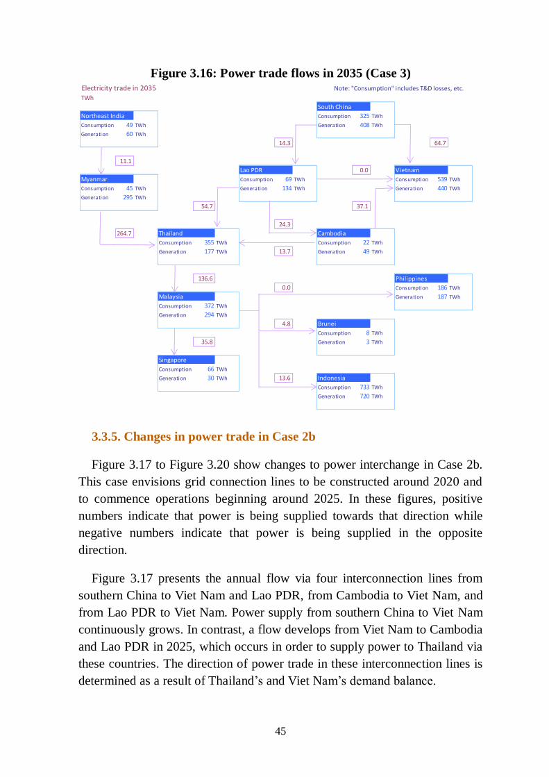
45

Figure 3.16: Power trade flows in 2035 (Case 3)

3.3.5. Changes in power trade in Case 2b

Figure 3.17 to Figure 3.20 show changes to power interchange in Case 2b.

This case envisions grid connection lines to be constructed around 2020 and

to commence operations beginning around 2025. In these figures, positive

numbers indicate that power is being supplied towards that direction while

negative numbers indicate that power is being supplied in the opposite

direction.

Figure 3.17 presents the annual flow via four interconnection lines from

southern China to Viet Nam and Lao PDR, from Cambodia to Viet Nam, and

from Lao PDR to Viet Nam. Power supply from southern China to Viet Nam

continuously grows. In contrast, a flow develops from Viet Nam to Cambodia

and Lao PDR in 2025, which occurs in order to supply power to Thailand via

these countries. The direction of power trade in these interconnection lines is

determined as a result of Thailand’s and Viet Nam’s demand balance.

Electricity trade in 2035 Note: "Consumption" includes T&D losses, etc.

TWh

South China

Northeast India Consumption 325 TWh

Consumption 49 TWh Generation 408 TWh

Generation 60 TWh

14.3 64.7

11.1

Lao PDR 0.0 Vietnam

Myanmar Consumption 69 TWh Consumption 539 TWh

Consumption 45 TWh Generation 134 TWh Generation 440 TWh

Generation 295 TWh

54.7 37.1

24.3

264.7 Thailand Cambodia

Consumption 355 TWh Consumption 22 TWh

Generation 177 TWh 13.7 Generation 49 TWh

136.6 Philippines

0.0 Consumption 186 TWh

Malaysia Generation 187 TWh

Consumption 372 TWh

Generation 294 TWh

4.8 Brunei

Consumption 8 TWh

35.8 Generation 3 TWh

Singapore

Consumption 66 TWh

Generation 30 TWh 13.6 Indonesia

Consumption 733 TWh

Generation 720 TWh

46

The ERIA Outlook sketches a scenario in which Viet Nam’s power supply

and demand grows the most rapidly as time moves towards 2035.

Consequently, in 2035, the trend reverses, and power is supplied from

Cambodia and Lao PDR to Viet Nam. Accompanying the expansion in supply

from southern China to Viet Nam is the decrease in the export of power from

southern China to Lao PDR towards 2035.

Figure 3.17: Changes in power trade in Case 2b (1)

Figure 3.18 shows the power supply from Myanmar, Lao PDR, Cambodia

and Malaysia to Thailand. As of 2025, Lao PDR is the largest supplier of

power to Thailand, followed by Myanmar and Cambodia. However,

accompanying the rapid expansion in Viet Nam’s demand, the supply coming

from Lao PDR and Cambodia begins to decrease and Myanmar assumes the

position of being the largest supplier towards 2035. Meanwhile, despite being

in a small net import position with Malaysia in 2025, Thailand will be in a

reverse position by 2035 as it begins to export power. As a result, as shown in

Figure 3.15, it becomes possible to supply hydro-potential power from the

northern regions to the southern regions, including Singapore. This will be

particularly noticeable around 2035 when supply in the south begins to run

short given the expanding demand in Indonesia.

-20

-10

0

10

20

30

40

50

60

70

2020 2025 2030 2035

TWh

YNN→VNM

YNN→LAO

KHM→VNM

LAO→VNM

47

-20

-15

-10

-5

0

5

10

15

2020 2025 2030 2035

TWh

MYS→IDN

MYS→SGP

MYS→BRN

MYS→THA

Figure 3.18: Changes in power trade in Case 2b (2)

Figure 3.19 presents the export from Malaysia to Singapore, Brunei,

Thailand and Indonesia. As this figure shows, Singapore and Brunei enjoy a

stable power supply via Malaysia. The countries providing the supply for that

are Indonesia and Thailand, but their supply amounts change over time.

Supply coming from Indonesia shrinks due to the rapid growth in domestic

demand. Accordingly, the reliance on northern hydro that passes through

Thailand increases. This region’s supply capacity itself is around 5-10TW and

is small in scale when compared to the supply and demand balance in the

northern region shown in Figure 3.17 and Figure 3.18 which center on

Thailand and Viet Nam.

Figure 3.19: Changes in power trade in Case 2b (3)

-10

0

10

20

30

40

50

60

70

80

90

2020 2025 2030 2035

TWh

MYA→THA

LAO→THA

KHM→THA

MYS→THA

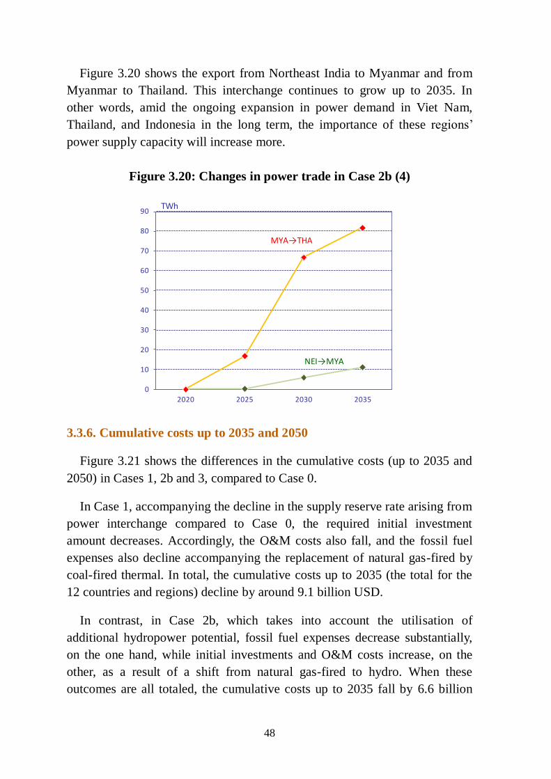
48

0

10

20

30

40

50

60

70

80

90

2020 2025 2030 2035

TWh

NEI→MYA

MYA→THA

Figure 3.20 shows the export from Northeast India to Myanmar and from

Myanmar to Thailand. This interchange continues to grow up to 2035. In

other words, amid the ongoing expansion in power demand in Viet Nam,

Thailand, and Indonesia in the long term, the importance of these regions’

power supply capacity will increase more.

Figure 3.20: Changes in power trade in Case 2b (4)

3.3.6. Cumulative costs up to 2035 and 2050

Figure 3.21 shows the differences in the cumulative costs (up to 2035 and

2050) in Cases 1, 2b and 3, compared to Case 0.

In Case 1, accompanying the decline in the supply reserve rate arising from

power interchange compared to Case 0, the required initial investment

amount decreases. Accordingly, the O&M costs also fall, and the fossil fuel

expenses also decline accompanying the replacement of natural gas-fired by

coal-fired thermal. In total, the cumulative costs up to 2035 (the total for the

12 countries and regions) decline by around 9.1 billion USD.

In contrast, in Case 2b, which takes into account the utilisation of

additional hydropower potential, fossil fuel expenses decrease substantially,

on the one hand, while initial investments and O&M costs increase, on the

other, as a result of a shift from natural gas-fired to hydro. When these

outcomes are all totaled, the cumulative costs up to 2035 fall by 6.6 billion

49

USD compared to Case 0, and increase by 2.5 billion USD compared to Case

1. In Case 3, where the usage of additional hydropower generation potential is

greater, there is a 3.8-billion USD decline in cumulative costs compared to

Case 0 and a 5.3-billion USD increase compared to Case 1.

The increase in cumulative costs up to 2035 accompanying the utilisation of

additional hydro points to the fact that it will not be possible to fully recover

the initial investment needed for hydropower generation facilities. If the

cumulative costs are evaluated over a longer time scale such as until 2050,

however, then the cumulative costs in Cases 2b and 3 will decline compared

to Case 1 because more of the initial investment for hydro will be recovered.

Therefore, the economies of constructing international interconnection lines

improves under systematic planning with a long-term perspective.

Figure 3.21: Cumulative costs in each case

3.4. Conclusion

This study uses an optimal power generation planning model that takes into

account international interconnection together with a supply reliability model

that employs the Monte Carlo method to analyse international grid connection

options up to 2035. Grid connections in the ASEAN region would reduce the

costs of the overall power system and bring massive benefits to the region

through effective utilisation of additional hydropower generation potential

and reduction of supply reserve margin. However, when it comes to utilising

additional hydro-thermal power potential, it might not be possible to recover

the initial investment required due to unavoidable barriers if the time scale is

-30,000

-20,000

-10,000

0

10,000

20,000

30,000

Case 0 Case 1 Case 2b Case 3

USD million

Initial Costs (- 2035)

O&M Costs (-2035)

Fuel Costs (-2035)

Total System Cost(cumulative to 2035)

Total System Cost(cumulative to 2050)

50

until 2035. Consequently, it is necessary to draw up plans with a longer time

scale that looks ahead to, say, 2050.

In this study a constant cost for additional hydro-potential was employed.

However, the fact is that the economics of hydropower generation changes

depending on location. As a result, there is a possibility that the feasibility of

hydro-potential shown in Chapter 2 will also differ. In the future, it will be

advantageous if a more realistic evaluation were to be done by assessing,

among others, the costs of each kind of power generation, most notably,

hydro-generation, and the grid connection costs for each region.

51

CHAPTER 4

PRELIMINARY ASSESSMENT OF POSSIBLE INTERCONNECTION

This chapter will select candidates for interconnection that would

conceivably be effective based on the considerations of the previous chapter,

and attempt to calculate the economic effects, including a rough estimation of

the cost of constructing interconnected transmission lines. After these

considerations, priorities are set for these selected interconnection lines.

4.1. Exploring interconnection cases

Based on the results from the previous chapter, interconnection lines that

appear to have significant advantages will be selected, and the economic

effects arising from each interconnection will be calculated and compared.

The main criterion for selection is the amount of estimated power flow.

Among a number of possible interconnection lines, the lines that are

estimated to have larger power flows than the others will be selected.

In this regard, the following cases were explored:

Case A: Thailand (THA) – Cambodia (KHM)

Case B: Thailand (THA) – Laos (LAO)

Case C: Thailand (THA) – Myanmar (MYA)

Case D: Myanmar (MYA) – Thailand (THA) – Malaysia (MYS) –

Singapore (SGP)

Case E: Viet Nam (VNM) – Laos (LAO) – Thailand (THA)

Case F: Malaysia (MYS) – Indonesia (IDN)

Case G: Laos (LAO) – Thailand (THA) – Malaysia (MYS) – Singapore

(SGP)

52

4.2. Route considerations for interconnected transmission lines

When considering a transmission system interconnection between two

countries, it is necessary to confirm the condition of the transmission systems

of each country in detail, and then decide the optimum connection points and

detailed interconnection routes. However, the goal of this study is a

preliminary assessment of the relationship between the effects of

interconnection and the cost. Hence, issues such as connection points and

detailed routes will be the subject of future investigation. Taking that into

consideration and given the need to determine routes as a reference for

transmission line costs, the most appropriate approach is to configure two

routes – a comparatively long-distance route and the shortest possible route –

and present the hypothetical costs as a range.

Based on this assumption, Route 1 shall be a comparatively long-distance

route linking capital cities, and Route 2 shall be linking short distance points

with existing substations wherever possible.

Additionally, because it is not possible to establish detailed routes in this

study, the transmission route length shall be set as 1.2 times the linear

distance between two points.

Figure 4.1: How routes are considered in each case

Route OptionRoute 1: Capital to Capital

Route 2: Nearest Route

Assumption of route lengthLinear Distance x 1.2

Route OptionRoute 1: Capital to Capital

Route 2: Nearest Route

Assumption of route lengthLinear Distance x 1.2

Route OptionRoute 1: Capital to Capital

Route 2: Nearest Route

Assumption of route lengthLinear Distance x 1.2

53

Linear

Distance

Route

Distance

[km] [km]

A THA-KHM Bangkok-Phnom Penh 530 636

B THA-LAO Bangkok-Vientiane 530 636

C THA-MYA Bangkok-Naypyidaw 800 960

D MYA-THA-MYS-SGP Naypyidaw-Bangkok 800 960

Bangkok-Kuala Lumpur 1350 1620

Kuala Lumpur-Singapore 350 420

E VNM-LAO-THA Hanoi-Vientiane 480 576

Vientiane-Bangkok 530 636

F MYS-IDN Kuala Lumpur-(coast of Malay Peninsula) 50 60

Malay Peninsula - Sumatra Island 90 108

in Sumatra Island 1200 1440

Sumatra Island - Java Island 50 60

(coast of Java Island)-Jakarta 120 144

G LAO-THA-MYS-SGP Vientiane-Bangkok 530 636

Bangkok-Kuala Lumpur 1350 1620

Kuala Lumpur-Singapore 350 420

Case Point Name

Linear

Distance

Route

Distance

[km] [km]

A THA-KHM Chanthaburi SS - Lower Stug Russey SS 100 120

B THA-LAO Ubon 3 SS - Ban Sok SS 200 240

C THA-MYA Mae Moh 3 SS - Yangon 450 540

D MYA-THA-MYS-SGP Yangon - Mae Moh 3 SS 450 540

Khlong Ngae SS - Gurun SS 110 132

Top of Malay Peninsula - Singapore 20 24

E VNM-LAO-THA Pleiku SS - Ban Sok SS 120 144

Ban Sok SS- Ubon 3 SS 200 240

F MYS-IDN Malay Peninsula - Sumatra Island 90 108

Sumatra Island - Java Island 50 60

G LAO-THA-MYS-SGP Ban Sok SS- Ubon 3 SS 200 240

Khlong Ngae SS - Gurun SS 110 132

Top of Malay Peninsula - Singapore 20 24

Route Point Name

The route lengths that were calculated on that basis are as follows:

Table 4.1: Route length calculation results (Route 1)

Table 4.2: Route length calculation results (Route 2)

54

4.3. Cost considerations for interconnected transmission lines

4.3.1. Cost components of interconnected transmission lines

When establishing interconnected transmission lines, the necessary costs

can be broadly categorised as 1) construction costs; and 2) operating and

maintenance (O&M) costs.

The cost of constructing transmission lines would generally be the cost of

obtaining (purchasing) the land, the cost of the materials (transmission towers,

electric cables, insulators, etc.), the construction labor costs, and so on.

However, these costs will change depending on various elements, including

the country, location, and environmental condition where the lines are being

constructed. For a rigorous cost estimate, it would be necessary to confirm

and configure each of those elements in detail. However, because this study

only involves a preliminary assessment, the construction costs are simplified.

That being the case, in preliminary assessments, the general approach taken

in calculating transmission line construction costs is to establish a unit

construction cost per unit length (1 km) and then multiply it with the route

length. This is also the approach taken in this study.

It should be pointed out that in all the cases, the interconnected

transmission lines to be constructed are assumed to be 500kV transmission

lines. The unit construction costs for overhead lines and undersea cables are

calculated and set based on actual market prices in recent years.

Where O&M costs are concerned, conceivable costs include the cost of

labor for regular patrols, the cost of fuel for traveling, the cost of materials

when making repairs, insurance costs when working in high places, and so on.

However, due to the difficulty in setting and adding up these costs in detail,

generally speaking again, in many cases, a certain annual amount is assumed

as the cost, and that amount is established as a fixed ratio of the construction

cost. As such, O&M costs in this study are established as an annual cost that

is 0.3 percent of the construction costs.

4.3.2. Setting unit construction costs

Unit construction costs (unit cost per km) were calculated as follows:

55

Figure 4.2 plots the actual contract costs of major transmission line

construction projects (500kV) in Southeast Asia in recent years (the past

decade) against the transmission line route lengths (two circuits for overhead

transmission lines and one circuit for undersea cable).

Figure 4.2: Actual transmission line construction costs in neighbouring

countries (500kV overhead lines)

Figure 4.3: Actual transmission line construction costs in neighbouring

countries (500kV undersea cable)

Seeking an average value by adding an approximate straight line to each

graph based on these data produced the following results:

<Overhead line>

56

According to the approximate line y=0.8633x, the cost is roughly 0.9

million USD/km/2 circuits overhead lines, so a unit construction cost figure

of 0.45 million USD/km/circuit overhead line is established.

<Undersea cable>

According to the approximate line y=4.4355x, the cost is roughly 4.5

million USD/km/1 circuit undersea cable, so a unit construction cost figure of

5 million USD/km/1 circuit undersea cable is established.

4.3.3. Setting conditions for alternative current (AC) transmission lines

Next, the following respective conditions are set as conditions for

calculating the construction costs of AC transmission lines. Note that AC

overhead lines should be applied to all of Cases A to E.

(1) Voltage

In the region that is subject to this study, 500kV transmission lines are

currently widely used as transmission lines for carrying large quantities of

power. For the purposes of this study, the interconnected transmission lines

shall also be considered as 500kV transmission lines in all cases.

(2) Transmission capacity

A single circuit power line (wire) has a threshold figure for the power it

can stably transmit. To carry power in excess of that threshold, it is

necessary to increase the number of circuits. As a result, the number of

circuits must be set according to the maximum amount of power that may

be carried.

This study assumes the use of wires that are commonly utilised in many

projects, and sets the transmission capacity per circuit at 1.8GW.

(3) Number of circuits

As stated in (2) above, it is necessary to set the number of circuits

according to the maximum power that may be carried. Usually, a spare

circuit is allocated to prevent accidental disconnection of electric power

flow. Thus, in addition to the number of circuits required to transmit the

maximum power, an additional circuit is added as a spare.

57

(4) Intermediate switching stations (or substations)

In the case of AC transmission lines, intermediate switching stations

are generally set up when the route length is long in order to stabilise the

voltage and partition circuits during accidents. This study assumes that

one switching station (or substation) is set up for every 160km.

Switching station construction costs were considered as follows:

(a) Cost components of switching station construction

The costs of constructing switching stations include the cost

needed to acquire and develop the land where the switching

stations will be located and the facilities and equipment costs

(including the installation cost). However, in order to simplify cost

estimation, land-related and common equipment costs are

consolidated as “fixed costs” and viewed as necessary costs

common to a single switching station. Meanwhile, costs associated

with the equipment required according to the number of circuits

are added to this as “additional costs,” with the total amount being

a sum of these components. For the additional cost, the unit cost

per circuit is multiplied by the number of circuits.

(b) Setting an amount for the fixed cost

The fixed cost will change according to the location of the

switching station and the equipment types, but for the purpose of

this study, it is necessary to estimate the cost on the safe side.

Examining actual cost of new substation construction projects in

neighbouring countries shows that in many cases, this fixed cost

component was around 10 million USD and is consequently

assumed here that:

Fixed cost = 20 million USD

(c) Setting an amount for the unit additional cost

Similarly, examining actual cases in neighbouring countries

shows that unit additional costs mostly fluctuated around several

million US dollars. Consequently, this study assumed that:

Unit additional cost = 10 million USD / line

(d) Switching station construction cost

Based on the above, the cost of constructing a switching station

is found using the following formula:

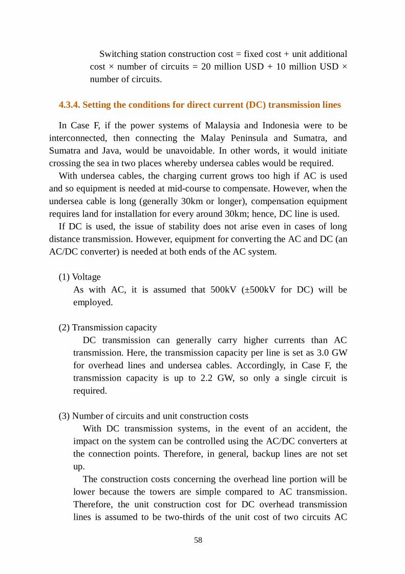
58

Switching station construction cost = fixed cost + unit additional

cost × number of circuits = 20 million USD + 10 million USD ×

number of circuits.

4.3.4. Setting the conditions for direct current (DC) transmission lines

In Case F, if the power systems of Malaysia and Indonesia were to be

interconnected, then connecting the Malay Peninsula and Sumatra, and

Sumatra and Java, would be unavoidable. In other words, it would initiate

crossing the sea in two places whereby undersea cables would be required.

With undersea cables, the charging current grows too high if AC is used

and so equipment is needed at mid-course to compensate. However, when the

undersea cable is long (generally 30km or longer), compensation equipment

requires land for installation for every around 30km; hence, DC line is used.

If DC is used, the issue of stability does not arise even in cases of long

distance transmission. However, equipment for converting the AC and DC (an

AC/DC converter) is needed at both ends of the AC system.

(1) Voltage

As with AC, it is assumed that 500kV (±500kV for DC) will be

employed.

(2) Transmission capacity

DC transmission can generally carry higher currents than AC

transmission. Here, the transmission capacity per line is set as 3.0 GW

for overhead lines and undersea cables. Accordingly, in Case F, the

transmission capacity is up to 2.2 GW, so only a single circuit is

required.

(3) Number of circuits and unit construction costs

With DC transmission systems, in the event of an accident, the

impact on the system can be controlled using the AC/DC converters at

the connection points. Therefore, in general, backup lines are not set

up.

The construction costs concerning the overhead line portion will be

lower because the towers are simple compared to AC transmission.

Therefore, the unit construction cost for DC overhead transmission

lines is assumed to be two-thirds of the unit cost of two circuits AC

59

No. of No. of Cost of

Circuit SS 1 SS

A THA-KHM Bangkok-Phnom Penh 3 3 50

B THA-LAO Bangkok-Vientiane 6 3 80

C THA-MYA Bangkok-Naypyidaw 8 5 100

D MYA-THA-MYS-SGP Naypyidaw-Bangkok 8 5 100 3,956

Bangkok-Kuala Lumpur 2 10 40 1,858

Kuala Lumpur-Singapore 2 2 40 458

E VNM-LAO-THA Hanoi-Vientiane 3 3 50 928

Vientiane-Bangkok 6 3 80 1,957

F MYS-IDN Kuala Lumpur-(coast of Malay Peninsula) 2 1 330 366

Malay Peninsula - Sumatra Island 1 0 302

in Sumatra Island 2 8 648

Sumatra Island - Java Island 1 0 168

(coast of Java Island)-Jakarta 2 1 330 416

G LAO-THA-MYS-SGP Vientiane – Bangkok 6 3 80 1,957

Bangkok – Kuala Lumpur 2 10 40 1,858 4,273

Kuala Lumpur – Singapore 2 2 40 458

1,957

3,956

6,272

2,885

1,901

Case Point NameConstruction Cost

[Mil USD]

1,009

lines (0.9 million USD/km) and is set at 0.6 million USD/km. With

regards to the undersea cable portion, the unit construction cost is set as

5 million USD/km, as found in section 4.3.2.

(4) AC/DC conversion stations

As stated above, DC transmission systems require installations of

AC/DC converters at the points of connection with the AC system.

Generally, these facilities resemble large substations, and the AC/DC

converters are costly. Here, a unit cost per 1 GW is set at 150 million

USD/GW. Because the transmission capacity in Case F is 2.2GW, the

cost per site will be 330 million USD.

With regards to the necessary number of converters, they will be

required at both ends (the Malaysia side and the Indonesia side) or at

two sites because with Route 1, DC transmission is to be applied on all

lines and with Route 2, they will be needed at both ends of the two

sections where crossing the sea takes place. Hence, a total of four sites

will be needed.

4.3.5. Cost calculation results

Based on the above assumptions, the construction costs that were

calculated for the interconnected transmission lines in the respective cases are

shown in Table 4.3.

Table 4.3: Transmission line construction costs (Route 1)

60

Table 4.4: Transmission line construction costs (Route 2)

4.4. Comparative calculation of benefits

Using the results above, the benefits of each case were calculated and

compared. In the previous chapter, the change in costs with or without

interconnection between the two countries was calculated for each case

(development cost increases for hydropower potential, reduced thermal power

generation fuel costs result from power interchange, and reduced power plant

development costs arise from lower reserve rates). The overall benefit

outcomes were calculated by adding the cost of interconnected transmission

lines.

Similar to the previous chapter’s cost calculations, the method for adding

the cost of the interconnected transmission lines was undertaken in the

following way:

The construction of the transmission lines was assumed to take place in

2025, with the full cost to be added that year.

The O&M cost was assumed to be added annually from the following

year of 2026.

A discount rate of 10 percent was assumed, and net present value at the

time of 2025 is calculated.

The difference compared for both cases -- [without interconnection]

minus [with interconnection] -- was calculated on a cumulative basis for

the 10-year period from 2025 to 2035.

* A plus value means gain in benefit.

No. of No. of Cost of

Circuit SS 1 SS

A THA-KHM Chanthaburi SS - Lower Stug Russey SS 3 0 50

B THA-LAO Ubon 3 SS - Ban Sok SS 6 1 80

C THA-MYA Mae Moh 3 SS - Yangon 8 3 100

D MYA-THA-MYS-SGP Yangon - Mae Moh 3 SS 8 3 100 2,244

Khlong Ngae SS - Gurun SS 2 0 40 119

2 0 40 22

E VNM-LAO-THA Pleiku SS - Ban Sok SS 3 0 50 194

Ban Sok SS- Ubon 3 SS 6 1 80 728

F MYS-IDN Malay Peninsula - Sumatra Island 3 0 50 962

Sumatra Island - Java Island 3 0 50 828

G LAO-THA-MYS-SGP Ban Sok SS- Ubon 3 SS 6 1 80 728

Khlong Ngae SS – Gurun SS 2 0 40 119

2 0 40 22

1790

162

728

2,244

2,384

922

868

Route Point NameConstruction Cost

[Mil USD]

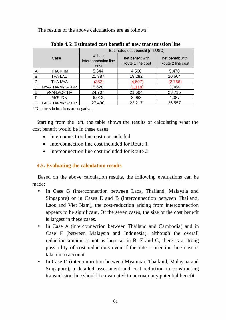
61

The results of the above calculations are as follows:

Table 4.5: Estimated cost benefit of new transmission line

* Numbers in brackets are negative.

Starting from the left, the table shows the results of calculating what the

cost benefit would be in these cases:

Interconnection line cost not included

Interconnection line cost included for Route 1

Interconnection line cost included for Route 2

4.5. Evaluating the calculation results

Based on the above calculation results, the following evaluations can be

made:

In Case G (interconnection between Laos, Thailand, Malaysia and

Singapore) or in Cases E and B (interconnection between Thailand,

Laos and Viet Nam), the cost-reduction arising from interconnection

appears to be significant. Of the seven cases, the size of the cost benefit

is largest in these cases.

In Case A (interconnection between Thailand and Cambodia) and in

Case F (between Malaysia and Indonesia), although the overall

reduction amount is not as large as in B, E and G, there is a strong

possibility of cost reductions even if the interconnection line cost is

taken into account.

In Case D (interconnection between Myanmar, Thailand, Malaysia and

Singapore), a detailed assessment and cost reduction in constructing

transmission line should be evaluated to uncover any potential benefit.

without

interconnection line

cost

net benefit with

Route 1 line cost

net benefit with

Route 2 line cost

A THA-KHM 5,644 4,560 5,470

B THA-LAO 21,387 19,282 20,604

C THA-MYA (352) (4,607) (2,766)

D MYA-THA-MYS-SGP 5,628 (1,118) 3,064

E VNM-LAO-THA 24,707 21,604 23,715

F MYS-IDN 6,012 3,968 4,087

G LAO-THA-MYS-SGP 27,490 23,217 26,557

Case

Estimated cost benefit [mil.USD]

62

In Case C (interconnection between Thailand and Myanmar), the cost

increases following hydropower development; thus, immediate benefit

from interconnected lines cannot be anticipated. However, it is possible

to anticipate further increase of benefit in the longer term.

Because this study is a preliminary assessment, the cost estimation is not

perfectly accurate. Therefore, while a comparative evaluation is possible to a

certain extent, a detailed and definitive evaluation is not possible at present.

In the future, it will therefore be necessary to utilise these cases and proceed

with a more detailed evaluation.

63

CHAPTER 5

KEY FINDINGS AND NEXT STEP

5.1. Key findings

The most fundamental thing that has been uncovered through this study is

how the entire region could benefit from the strengthening of international

grid interconnections. Within this region, there is a trend towards a

widespread increase in power demand. But the situation relating to the

presence of fuel resources for power generation differs from country to

country. For that reason, while one country may be blessed with abundant

resources, another country may have no choice but to rely on imports. Where

relationships among neighbouring countries are adversarial, each country has

no choice but to fulfil its own demand entirely with domestic supply.

However, given the trend towards promoting economic integration within this

region, from an economic perspective, it is more logical to find a balance

between power supply and demand at a regional level rather than at an

individual country level.

More specifically, in Laos, Cambodia, Myanmar and China’s Yunnan

Province, there is great potential for hydro power generation. Although the

cost of hydraulic power generation varies greatly by location, in many cases,

it is competitive with natural gas-fired power generation and coal-fired power

generation. Furthermore, in terms of making a response to the problem of

climate change, there is demand for the use of energy sources with the

smallest possible carbon footprint. On that point, hydraulic power generation

is thought to be an appropriate choice. In order to make the greatest possible

use of this latent resource, there is a need for a regional interconnected power

system.

In addition, utilising the different power demand patterns of each country, it

is possible to reduce the cost of the power supply throughout the entire region.

If a country is to meet its power demand on its own, it must maintain a

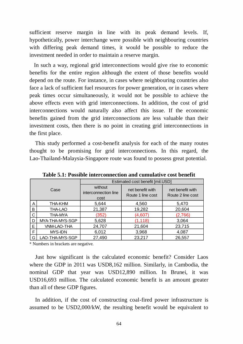
64

sufficient reserve margin in line with its peak demand levels. If,

hypothetically, power interchange were possible with neighbouring countries

with differing peak demand times, it would be possible to reduce the

investment needed in order to maintain a reserve margin.

In such a way, regional grid interconnections would give rise to economic

benefits for the entire region although the extent of those benefits would

depend on the route. For instance, in cases where neighbouring countries also

face a lack of sufficient fuel resources for power generation, or in cases where

peak times occur simultaneously, it would not be possible to achieve the

above effects even with grid interconnections. In addition, the cost of grid

interconnections would naturally also affect this issue. If the economic

benefits gained from the grid interconnections are less valuable than their

investment costs, then there is no point in creating grid interconnections in

the first place.

This study performed a cost-benefit analysis for each of the many routes

thought to be promising for grid interconnections. In this regard, the

Lao-Thailand-Malaysia-Singapore route was found to possess great potential.

Table 5.1: Possible interconnection and cumulative cost benefit

* Numbers in brackets are negative.

Just how significant is the calculated economic benefit? Consider Laos

where the GDP in 2011 was USD8,162 million. Similarly, in Cambodia, the

nominal GDP that year was USD12,890 million. In Brunei, it was

USD16,693 million. The calculated economic benefit is an amount greater

than all of these GDP figures.

In addition, if the cost of constructing coal-fired power infrastructure is

assumed to be USD2,000/kW, the resulting benefit would be equivalent to

without

interconnection line

cost

net benefit with

Route 1 line cost

net benefit with

Route 2 line cost

A THA-KHM 5,644 4,560 5,470

B THA-LAO 21,387 19,282 20,604

C THA-MYA (352) (4,607) (2,766)

D MYA-THA-MYS-SGP 5,628 (1,118) 3,064

E VNM-LAO-THA 24,707 21,604 23,715

F MYS-IDN 6,012 3,968 4,087

G LAO-THA-MYS-SGP 27,490 23,217 26,557

Case

Estimated cost benefit [mil.USD]

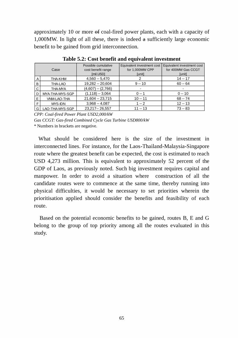
65

approximately 10 or more of coal-fired power plants, each with a capacity of

1,000MW. In light of all these, there is indeed a sufficiently large economic

benefit to be gained from grid interconnection.

Table 5.2: Cost benefit and equivalent investment

CPP: Coal-fired Power Plant USD2,000/kW

Gas CCGT: Gas-fired Combined Cycle Gas Turbine USD800/kW

* Numbers in brackets are negative.

What should be considered here is the size of the investment in

interconnected lines. For instance, for the Laos-Thailand-Malaysia-Singapore

route where the greatest benefit can be expected, the cost is estimated to reach

USD 4,273 million. This is equivalent to approximately 52 percent of the

GDP of Laos, as previously noted. Such big investment requires capital and

manpower. In order to avoid a situation where construction of all the

candidate routes were to commence at the same time, thereby running into

physical difficulties, it would be necessary to set priorities wherein the

prioritisation applied should consider the benefits and feasibility of each

route.

Based on the potential economic benefits to be gained, routes B, E and G

belong to the group of top priority among all the routes evaluated in this

study.

Possible cumulative

cost benefit range

[mil.USD]

Equivalent investment cost

for 1,000MW CPP

[unit]

Equivalent investment cost

for 400MW Gas CCGT

[unit]

A THA-KHM 4,560 -- 5,470 2 14 -- 17

B THA-LAO 19,282 -- 20,604 9 -- 10 60 -- 64

C THA-MYA (4,607) -- (2,766) - -

D MYA-THA-MYS-SGP (1,118) -- 3,064 0 -- 1 0 -- 10

E VNM-LAO-THA 21,604 -- 23,715 10 -- 11 68 -- 74

F MYS-IDN 3,968 -- 4,087 1 -- 2 12 -- 13

G LAO-THA-MYS-SGP 23,217-- 26,557 11 -- 13 73 -- 83

Case

66

Table 5.3: Possible interconnection line and their priority

* Numbers in brackets are negative.

Plans are already set in motion by the HAPUA to realize a grid

interconnection in ASEAN. Thus, there is a need to confirm whether the

candidate lines selected by this study conform with the plans that HAPUA is

currently advancing.

It should be noted that first and foremost, each of the routes selected by

this study has also been proposed by HAPUA. Second, the largest total

transmission capacity of any of the lines currently under construction in the

HAPUA plans is that of the Viet Nam-Laos-Thailand line, the same priority

plan proposed by this study. And third, this study and HAPUA conform in

terms of the recognition of a Thailand-Myanmar line as a future

interconnection candidate.

Beyond the above, however, there is a need to establish the differences in

the methodology employed by this study as compared to that of HAPUA.

This study is the result of analysis focused only on economic considerations.

On the other hand, HAPUA’s assessment took into account another criterion

meant to evaluate benefits of new interconnections beyond the economic

realm. . For instance, even if a line does not produce as large an economic

benefit as other lines, if it contributes to regional economic integration and

the power supply, there are instances where that line might receive high

prioritisation in the HAPUA plans. Indeed, decisions on selecting the

appropriate interconnected lines should be based on a comprehensive set of

criteria that considers a variety of aspects in addition to economic reasons.

Despite the slightly different approach, the results of this study can be said

to generally conform with the plan being promoted by HAPUA. In addition,

Possible cumulative cost

benefit range

[mil.USD]

Estimated cost of

trasmission line

[mil USD]

A THA-KHM 4,560 -- 5,470 162 -- 1,009 second priority

B THA-LAO 19,282 -- 20,604 728 -- 1,957 first priority

C THA-MYA (4,607) -- (2,766) 2,244 -- 3,956 need careful assess.

D MYA-THA-MYS-SGP (1,118) -- 3,064 2,384 -- 6,272 need careful assess.

E VNM-LAO-THA 21,604 -- 23,715 922 -- 2,885 first priority

F MYS-IDN 3,968 -- 4,087 1,790 -- 1,901 second priority

G LAO-THA-MYS-SGP 23,217-- 26,557 868 -- 4,273 first priority

Case

67

while HAPUA’s construction plans generally set a target of 2020, this study

considers the accumulated benefit from 2020 to 2035, and is thus an

extension of the HAPUA plans.

Table 5.4: HAPUA lead plan

Source: HAPUA

Based on the above analysis, this study makes the following proposals.

Accelerate construction of the Viet Nam – Laos – Thailand – Malaysia -

Singapore interconnection line.

Place increased priority on the Thailand-Cambodia line.

Going back to the premise of this study, the economic benefit to be gained

from the Viet Nam-Laos-Thailand-Malaysia-Singapore line is huge. There

already exists a transmission link connecting these countries and plans are

underway to reinforce that line. However, in order to enjoy the benefits that

would arise from such an interconnection line to the greatest extent possible, it

is desirable to further enhance transmission capacity and accelerate

construction.

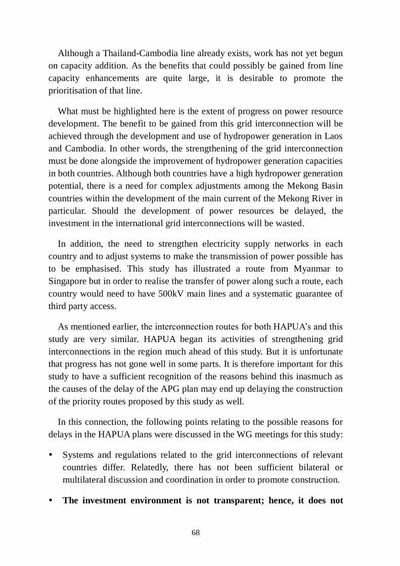
68

Although a Thailand-Cambodia line already exists, work has not yet begun

on capacity addition. As the benefits that could possibly be gained from line

capacity enhancements are quite large, it is desirable to promote the

prioritisation of that line.

What must be highlighted here is the extent of progress on power resource

development. The benefit to be gained from this grid interconnection will be

achieved through the development and use of hydropower generation in Laos

and Cambodia. In other words, the strengthening of the grid interconnection

must be done alongside the improvement of hydropower generation capacities

in both countries. Although both countries have a high hydropower generation

potential, there is a need for complex adjustments among the Mekong Basin

countries within the development of the main current of the Mekong River in

particular. Should the development of power resources be delayed, the

investment in the international grid interconnections will be wasted.

In addition, the need to strengthen electricity supply networks in each

country and to adjust systems to make the transmission of power possible has

to be emphasised. This study has illustrated a route from Myanmar to

Singapore but in order to realise the transfer of power along such a route, each

country would need to have 500kV main lines and a systematic guarantee of

third party access.

As mentioned earlier, the interconnection routes for both HAPUA’s and this

study are very similar. HAPUA began its activities of strengthening grid

interconnections in the region much ahead of this study. But it is unfortunate

that progress has not gone well in some parts. It is therefore important for this

study to have a sufficient recognition of the reasons behind this inasmuch as

the causes of the delay of the APG plan may end up delaying the construction

of the priority routes proposed by this study as well.

In this connection, the following points relating to the possible reasons for

delays in the HAPUA plans were discussed in the WG meetings for this study:

Systems and regulations related to the grid interconnections of relevant

countries differ. Relatedly, there has not been sufficient bilateral or

multilateral discussion and coordination in order to promote construction.

The investment environment is not transparent; hence, it does not

69

attract sufficient private companies and foreign capital. Accordingly,

there has not been a sufficient provision of capital.

Because the framework devised by HAPUA does not pursue economic

benefits alone, the plan is unable to gather sufficient investments in the form of

private and foreign capital. Therefore, direct and indirect participation by

governments, including construction by public power companies, becomes

indispensable.

In light of this, there is room for improvement in terms of relations between

countries. For instance, in Europe, the European Commission (EC) is

constructing unified regulation and market systems with the goal of achieving

increasing benefits for all member states. In addition, the EC is also unifying

regional power markets as well as selecting routes for which construction

should be prioritised in order to improve the stability of supply. It is also

offering capital support for this. It is believed that interstate frameworks are

functioning effectively for the construction of a region-wide power

transmission network running across national borders.

In the EAS region, the creation of a framework with the goal of streamlining

the enhancement of benefits for the entire region could be expected to

encourage the creation of grid interconnections. Specifically, taking the

European experience as a case study, there is a group comprising the regulating

bodies of each country, and a group comprising the power transmission

companies of each country. These groups set the common regulations they

believe should be applied, create common development plans, and set

obligations that each country within the region is expected to equally follow.

Because each county would have to relinquish part of its own market

regulatory functions for this, there would likely be strong resistance to the

formulation of such a system. However, this can also be said to be the logical

choice, building on the great push towards the creation of the ASEAN

Economic Community in 2015.

5.2. Next Step

Based on the results of the quantitative analysis done in this study of the

potential economic benefits and costs stemming from international grid

interconnections based on certain preconditions, a number of priority routes

were selected.

70

It is hoped that ultimately, actual investments will be made to realise the

construction of these routes and to reap the benefits expected to be gained.

While the results of the analysis in this research may lead to further

discussion and decisions, it has to be acknowledged that a number of issues

had been insufficiently addressed in this study. For instance, there has to be a

closer examination of the route selection for power transmission lines and of

the cost calculations. In addition, certain barriers in terms of policies and,

technology, among others, are believed to exist that affect the actual

realisation of grid interconnections. These issues need to be addressed

because the reliability of the analysis of this research would be improved by

addressing these points which have been insufficiently analyzed at the

moment. That is therefore the next step. And it is hoped that the improvement

of the validity of this analysis will create an opportunity for the realization of

investment. That is the direction aimed at by this study.

71

Appendix 1. Power generation mix in each case (2035)

(Case 0: 2035)

(Case 1: 2035)

(Case 2a: 2035)

Unit: TWh

SGP BRN IDN MYS PHL THA VNM MYA LAO KHM YNN NEI Total

Coal 0 0 316 187 133 49 322 8 14 7 88 3 1,126

Oil 0 0 0 0 0 0 0 0 1 0 0 0 1

Natural gas 61 8 231 166 31 254 136 21 0 0 49 31 989

Hydro 0 0 92 18 8 4 51 11 54 15 187 15 457

Nuclear & geothermal 0 0 65 0 12 23 29 0 0 0 0 0 128

Others 5 0 29 0 1 26 0 4 0 0 0 0 66

Net imports 0 0 0 0 0 0 0 0 0 0 0 0 0

Total 66 8 733 372 186 355 539 45 69 22 325 49 2,767

Unit: TWh

SGP BRN IDN MYS PHL THA VNM MYA LAO KHM YNN NEI Total

Coal 0 0 315 157 133 49 316 17 41 14 96 3 1,141

Oil 0 0 0 0 0 0 0 0 0 0 0 0 0

Natural gas 53 6 239 195 32 225 141 14 0 0 45 30 978

Hydro 0 0 92 18 8 4 51 11 54 15 187 15 457

Nuclear & geothermal 0 0 65 0 12 23 29 0 0 0 0 0 128

Others 5 0 29 0 1 26 0 4 0 0 0 0 66

Net imports 8 2 -6 1 -1 29 2 -2 -26 -7 -3 1 -2

Total 66 8 733 372 186 355 539 45 69 22 325 49 2,767

Unit: TWh

SGP BRN IDN MYS PHL THA VNM MYA LAO KHM YNN NEI Total

Coal 0 0 182 91 109 48 119 0 29 3 82 0 662

Oil 0 0 0 0 0 0 0 0 0 0 0 0 0

Natural gas 53 6 201 189 33 128 85 0 0 0 0 0 695

Hydro 0 0 265 88 32 16 240 95 81 35 319 56 1,227

Nuclear & geothermal 0 0 65 0 12 23 29 0 0 0 0 0 128

Others 5 0 29 0 1 26 0 4 0 0 0 0 66

Net imports 8 2 -9 4 -1 115 65 -55 -41 -16 -76 -8 -12

Total 66 8 733 372 186 355 539 45 69 22 325 49 2,767

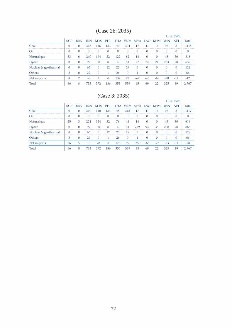
72

(Case 2b: 2035)

(Case 3: 2035)

Unit: TWh

SGP BRN IDN MYS PHL THA VNM MYA LAO KHM YNN NEI Total

Coal 0 0 313 146 133 49 304 17 41 14 96 3 1,115

Oil 0 0 0 0 0 0 0 0 0 0 0 0 0

Natural gas 53 6 240 194 32 122 82 14 0 0 45 30 818

Hydro 0 0 92 30 8 4 51 77 74 24 264 28 652

Nuclear & geothermal 0 0 65 0 12 23 29 0 0 0 0 0 128

Others 5 0 29 0 1 26 0 4 0 0 0 0 66

Net imports 8 2 -6 2 -1 132 72 -67 -46 -16 -80 -11 -12

Total 66 8 733 372 186 355 539 45 69 22 325 49 2,767

Unit: TWh

SGP BRN IDN MYS PHL THA VNM MYA LAO KHM YNN NEI Total

Coal 0 0 310 140 133 48 315 17 41 14 96 3 1,117

Oil 0 0 0 0 0 0 0 0 0 0 0 0 0

Natural gas 25 3 224 124 32 76 44 14 0 0 45 30 616

Hydro 0 0 92 30 8 4 51 259 93 35 268 28 868

Nuclear & geothermal 0 0 65 0 12 23 29 0 0 0 0 0 128

Others 5 0 29 0 1 26 0 4 0 0 0 0 66

Net imports 36 5 13 78 -1 178 99 -250 -65 -27 -83 -11 -28

Total 66 8 733 372 186 355 539 45 69 22 325 49 2,767

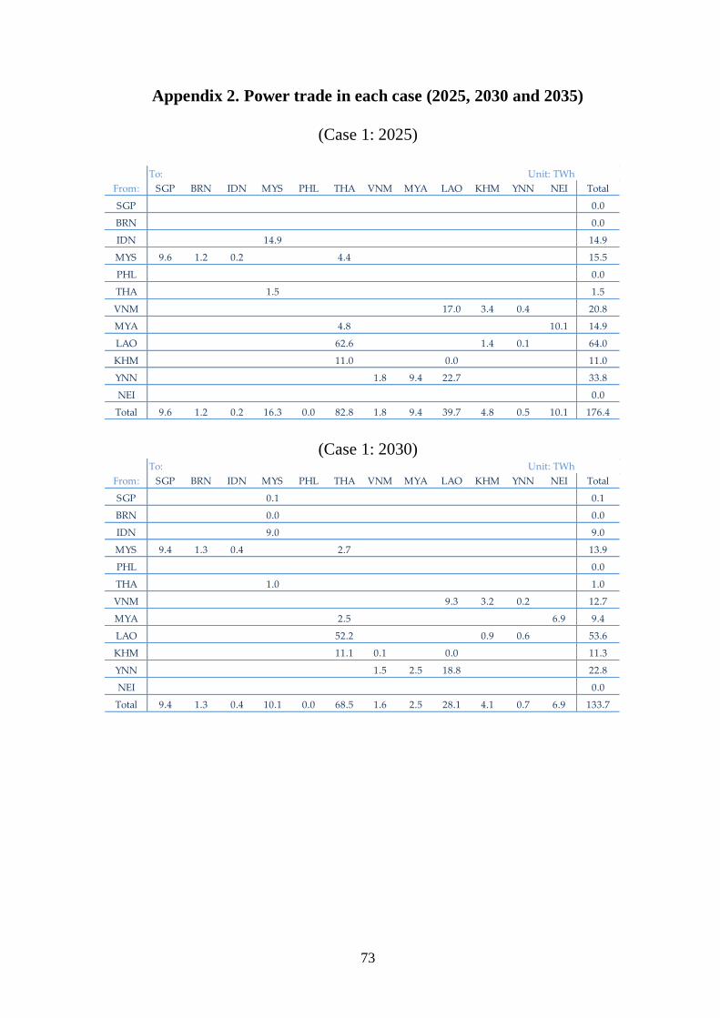
73

Appendix 2. Power trade in each case (2025, 2030 and 2035)

(Case 1: 2025)

(Case 1: 2030)

To: Unit: TWh

From: SGP BRN IDN MYS PHL THA VNM MYA LAO KHM YNN NEI Total

SGP 0.0

BRN 0.0

IDN 14.9 14.9

MYS 9.6 1.2 0.2 4.4 15.5

PHL 0.0

THA 1.5 1.5

VNM 17.0 3.4 0.4 20.8

MYA 4.8 10.1 14.9

LAO 62.6 1.4 0.1 64.0

KHM 11.0 0.0 11.0

YNN 1.8 9.4 22.7 33.8

NEI 0.0

Total 9.6 1.2 0.2 16.3 0.0 82.8 1.8 9.4 39.7 4.8 0.5 10.1 176.4

To: Unit: TWh

From: SGP BRN IDN MYS PHL THA VNM MYA LAO KHM YNN NEI Total

SGP 0.1 0.1

BRN 0.0 0.0

IDN 9.0 9.0

MYS 9.4 1.3 0.4 2.7 13.9

PHL 0.0

THA 1.0 1.0

VNM 9.3 3.2 0.2 12.7

MYA 2.5 6.9 9.4

LAO 52.2 0.9 0.6 53.6

KHM 11.1 0.1 0.0 11.3

YNN 1.5 2.5 18.8 22.8

NEI 0.0

Total 9.4 1.3 0.4 10.1 0.0 68.5 1.6 2.5 28.1 4.1 0.7 6.9 133.7

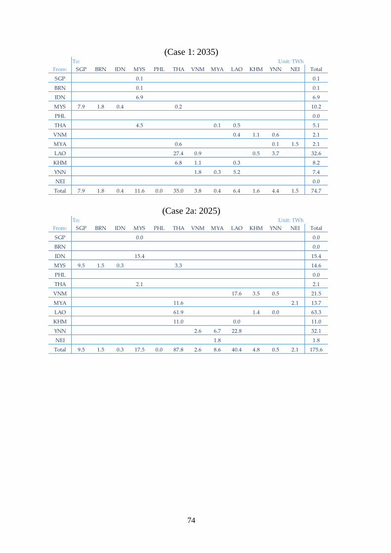
74

(Case 1: 2035)

(Case 2a: 2025)

To: Unit: TWh

From: SGP BRN IDN MYS PHL THA VNM MYA LAO KHM YNN NEI Total

SGP 0.1 0.1

BRN 0.1 0.1

IDN 6.9 6.9

MYS 7.9 1.8 0.4 0.2 10.2

PHL 0.0

THA 4.5 0.1 0.5 5.1

VNM 0.4 1.1 0.6 2.1

MYA 0.6 0.1 1.5 2.1

LAO 27.4 0.9 0.5 3.7 32.6

KHM 6.8 1.1 0.3 8.2

YNN 1.8 0.3 5.2 7.4

NEI 0.0

Total 7.9 1.8 0.4 11.6 0.0 35.0 3.8 0.4 6.4 1.6 4.4 1.5 74.7

To: Unit: TWh

From: SGP BRN IDN MYS PHL THA VNM MYA LAO KHM YNN NEI Total

SGP 0.0 0.0

BRN 0.0

IDN 15.4 15.4

MYS 9.5 1.5 0.3 3.3 14.6

PHL 0.0

THA 2.1 2.1

VNM 17.6 3.5 0.5 21.5

MYA 11.6 2.1 13.7

LAO 61.9 1.4 0.0 63.3

KHM 11.0 0.0 11.0

YNN 2.6 6.7 22.8 32.1

NEI 1.8 1.8

Total 9.5 1.5 0.3 17.5 0.0 87.8 2.6 8.6 40.4 4.8 0.5 2.1 175.6

75

(Case 2a: 2030)

(Case 2a: 2035)

To: Unit: TWh

From: SGP BRN IDN MYS PHL THA VNM MYA LAO KHM YNN NEI Total

SGP 0.2 0.2

BRN 0.0 0.0

IDN 8.9 8.9

MYS 9.4 1.5 0.4 1.1 12.4

PHL 0.0

THA 2.2 0.0 2.3

VNM 4.1 2.5 0.3 6.9

MYA 39.3 1.0 40.3

LAO 53.9 0.2 1.0 0.6 55.6

KHM 14.6 0.2 0.1 14.8

YNN 7.6 2.1 12.8 22.6

NEI 4.3 4.3

Total 9.4 1.5 0.4 11.3 0.0 108.9 8.0 6.4 16.9 3.5 0.9 1.0 168.1

To: Unit: TWh

From: SGP BRN IDN MYS PHL THA VNM MYA LAO KHM YNN NEI Total

SGP 0.2 0.2

BRN 0.1 0.1

IDN 9.2 9.2

MYS 8.0 1.8 0.4 0.6 10.8

PHL 0.0

THA 5.6 0.1 5.7

VNM 0.0

MYA 65.9 0.4 0.5 66.8

LAO 46.7 4.9 0.2 0.7 52.6

KHM 12.9 2.8 0.2 15.9

YNN 60.1 4.4 11.8 76.4

NEI 8.0 8.0

Total 8.0 1.8 0.4 15.0 0.0 126.1 67.8 12.4 12.1 0.2 1.1 0.5 245.4

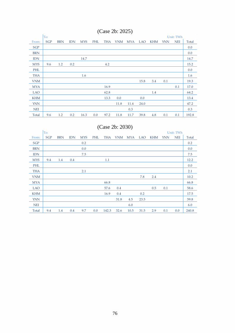
76

(Case 2b: 2025)

(Case 2b: 2030)

To: Unit: TWh

From: SGP BRN IDN MYS PHL THA VNM MYA LAO KHM YNN NEI Total

SGP 0.0

BRN 0.0

IDN 14.7 14.7

MYS 9.6 1.2 0.2 4.2 15.2

PHL 0.0

THA 1.6 1.6

VNM 15.8 3.4 0.1 19.3

MYA 16.9 0.1 17.0

LAO 62.8 1.4 64.2

KHM 13.3 0.0 0.0 13.4

YNN 11.8 11.4 24.0 47.2

NEI 0.3 0.3

Total 9.6 1.2 0.2 16.3 0.0 97.2 11.8 11.7 39.8 4.8 0.1 0.1 192.8

To: Unit: TWh

From: SGP BRN IDN MYS PHL THA VNM MYA LAO KHM YNN NEI Total

SGP 0.2 0.2

BRN 0.0 0.0

IDN 7.5 7.5

MYS 9.4 1.4 0.4 1.1 12.2

PHL 0.0

THA 2.1 2.1

VNM 7.8 2.4 10.2

MYA 66.8 66.8

LAO 57.6 0.4 0.5 0.1 58.6

KHM 16.9 0.4 0.2 17.5

YNN 31.8 4.5 23.5 59.8

NEI 6.0 6.0

Total 9.4 1.4 0.4 9.7 0.0 142.3 32.6 10.5 31.5 2.9 0.1 0.0 240.8

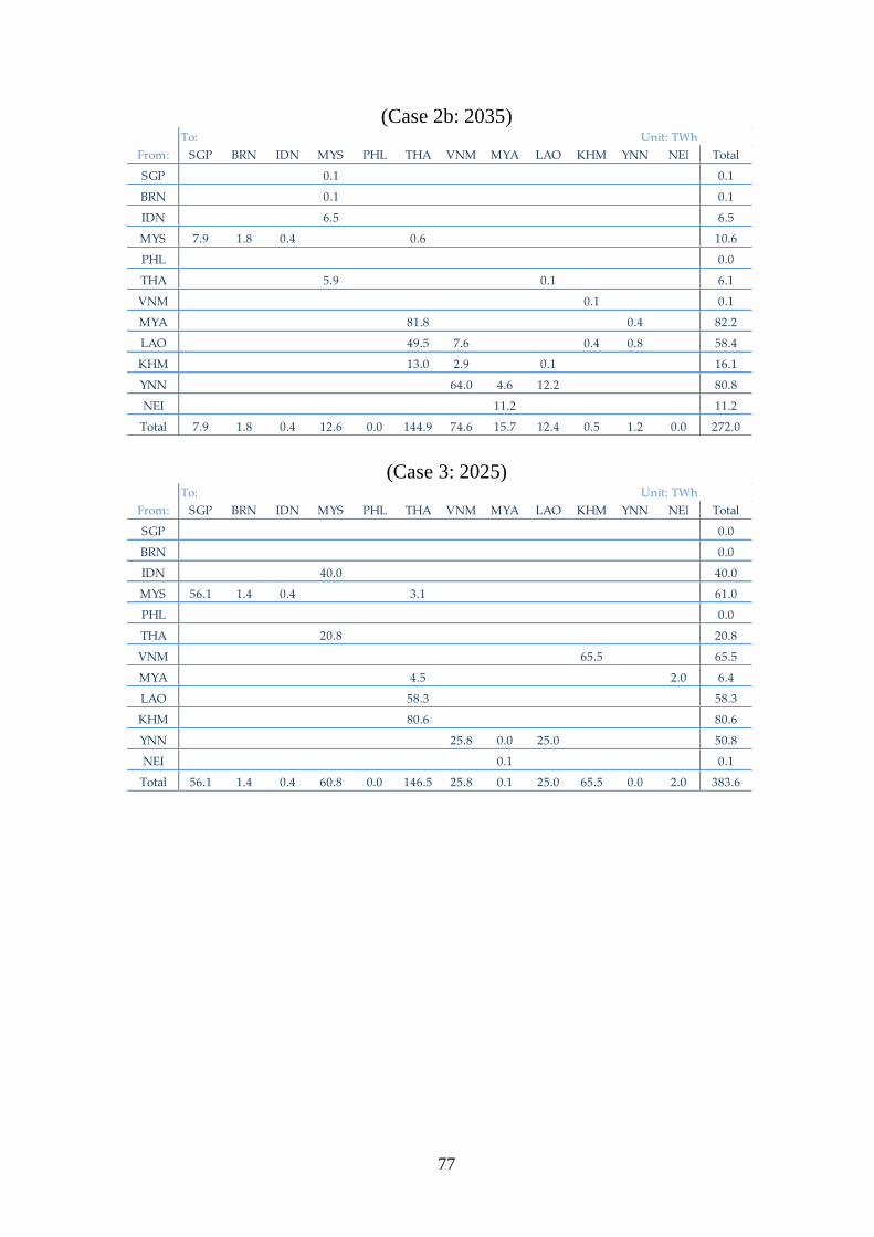
77

(Case 2b: 2035)

(Case 3: 2025)

To: Unit: TWh

From: SGP BRN IDN MYS PHL THA VNM MYA LAO KHM YNN NEI Total

SGP 0.1 0.1

BRN 0.1 0.1

IDN 6.5 6.5

MYS 7.9 1.8 0.4 0.6 10.6

PHL 0.0

THA 5.9 0.1 6.1

VNM 0.1 0.1

MYA 81.8 0.4 82.2

LAO 49.5 7.6 0.4 0.8 58.4

KHM 13.0 2.9 0.1 16.1

YNN 64.0 4.6 12.2 80.8

NEI 11.2 11.2

Total 7.9 1.8 0.4 12.6 0.0 144.9 74.6 15.7 12.4 0.5 1.2 0.0 272.0

To: Unit: TWh

From: SGP BRN IDN MYS PHL THA VNM MYA LAO KHM YNN NEI Total

SGP 0.0

BRN 0.0

IDN 40.0 40.0

MYS 56.1 1.4 0.4 3.1 61.0

PHL 0.0

THA 20.8 20.8

VNM 65.5 65.5

MYA 4.5 2.0 6.4

LAO 58.3 58.3

KHM 80.6 80.6

YNN 25.8 0.0 25.0 50.8

NEI 0.1 0.1

Total 56.1 1.4 0.4 60.8 0.0 146.5 25.8 0.1 25.0 65.5 0.0 2.0 383.6

78

(Case 3: 2030)

(Case 3: 2035)

To: Unit: TWh

From: SGP BRN IDN MYS PHL THA VNM MYA LAO KHM YNN NEI Total

SGP 0.0

BRN 0.0 0.0

IDN 16.4 16.4

MYS 58.7 1.7 1.5 61.9

PHL 0.0

THA 46.6 46.6

VNM 46.0 46.0

MYA 77.0 77.0

LAO 74.6 0.0 74.6

KHM 67.3 0.6 67.9

YNN 38.5 1.1 25.3 64.9

NEI 6.0 6.0

Total 58.7 1.7 1.5 63.0 0.0 218.8 39.1 7.1 25.3 46.0 0.0 0.0 461.0

To: Unit: TWh

From: SGP BRN IDN MYS PHL THA VNM MYA LAO KHM YNN NEI Total

SGP 0.0

BRN 0.0

IDN 0.6 0.6

MYS 35.8 4.8 14.2 54.8

PHL 0.0

THA 136.6 0.6 137.2

VNM 5.7 5.7

MYA 264.7 264.7

LAO 54.7 24.3 78.9

KHM 14.3 42.8 57.1

YNN 64.7 4.5 14.3 83.5

NEI 11.1 11.1

Total 35.8 4.8 14.2 137.2 0.0 333.6 107.5 15.6 14.3 30.5 0.0 0.0 693.6

79

Appendix 3. Cumulative costs up to 2035

(differences compared to Case 0)

Unit: USD million

Case 0 Case 1 Case 2b Case 3

Initial cost 0 -3,308 6,276 16,482

Fuel cost 0 -3,882 -15,790 -27,070

O&M cost 0 -1,883 2,952 6,827

Total cost 0 -9,073 -6,562 -3,761