INVESTIGATION ON EFFECTIVE MODULUS AND STRESS

i

INVESTIGATION ON EFFECTIVE MODULUS AND STRESS CONCENTRATION

FACTOR OF 3D REINFORCED COMPOSITE BY FINITE

ELEMENT ANALYSIS METHOD

by

CHANDRA BHASKAR REDDY PITTU

Presented to the Faculty of the Graduate School of

The University of Texas at Arlington in Partial Fulfillment

of the Requirements

for the Degree of

MASTER OF SCIENCE IN MECHANICAL ENGINEERING

THE UNIVERSITY OF TEXAS AT ARLINGTON

May 2018

ii

Copyright © by Chandra Bhaskar Reddy Pittu 2018

All Rights Reserved

iii

Acknowledgements

I owe deep gratitude to my family without whose support and encouragements this

wouldn’t have been possible.

I would like to thank my thesis guide Dr. Andrey Beyle, for guiding me throughout

the years with his time, ideas, insightful comments and stimulating discussions on various

topics during my thesis work. It has been an incredible journey and a great experience

working with him on research projects. His guidance helped me in all the time of research

and writing of this thesis. I could not have imagined having a better advisor and mentor for

my thesis study. I would also like to thank him for his encouragement to help me cross all

the obstacles.

I would also like to thank Dr. Robert Taylor and Dr. Dereje Agonafer for serving on

my committee and providing numerous learning opportunities by their insightful comments

and hard questions. I would like to extend a special Thanks to Late Dr. Wen S Chan for his

great insights and teachings that helped me to develop interests in the field of composites

without which it could not have been possible to complete this Thesis.

I acknowledge the support provided by the FABLAB staff and Student Co-

Employees in the toughest times of managing and helping me around work for

accomplishing this thesis.

Finally, I would like to express my appreciation to all my friends in UTA and all the

people from Mechanical and Aerospace Engineering Department who made my time in

Arlington memorable.

.

April 30, 2018

iv

Abstract

INVESTIGATION OF EFFECTIVE MODULUS AND STRESS CONCENTRATION

FACTOR OF 3D REINFORCED COMPOSITE BY FINITE

ELEMENT ANALYSIS METHOD

Chandra Bhaskar Reddy Pittu, MS

The University of Texas at Arlington, 2018

Supervising Professor: Andrey Beyle

Micromechanics of Composites aims to analyze the localized stresses inside any

given constituents of the composite structure. This Thesis is focused on Calculating the

effective modulus and the Stress concentration factor of the 3D straight Fiber Composite

using Finite Element(FE). The compressive and a Shear response of a 3D Straight fiber

composite comprising three directional E Glass Fibers reinforced in an epoxy matrix is

analysed. This result is the 10% of overall Composite Ductility and a 10% of overall Shear

displacement load in the orthogonal directions. FE calculations are reported to analyse the

response of 3d reinforcement as of with the reduced fiber volume fractions in the respective

orthogonal directions. The FE calculations demonstrate that the three dimensionality of the

microstructure constrains the kinks, and this results in the stable load response. Integrated

Stresses of Constituents are formulated by FE to calculate the Effective Modulus and then

Stress concentration factor(SCF) to understand the behavior along the orthogonally varied

volume fraction models.

SCF Gives us the vital information on how concentrated the stress are in loaded

constituents when there is change in volume fraction orthogonally and would help in

predicting the failure methods and fatigue life of the material. .

v

Table of Contents

Acknowledgements .............................................................................................................iii

Abstract .............................................................................................................................. iv

List of Illustrations ..............................................................................................................vii

List of Tables ...................................................................................................................... xi

1 Chapter INTRODUCTION .......................................................................................... 1

1.1 Classification of Composites ............................................................................. 3

1.2 Need of 3D Composites .................................................................................... 6

1.3 Objective ............................................................................................................ 7

1.3.1 Motivation ...................................................................................................... 7

1.3.2 Goal and Objective ........................................................................................ 7

2 Chapter LITERATURE REVIEW ................................................................................ 9

3 Chapter MATERIAL CHARACTERISATION ........................................................... 14

3.1 MATRIX ........................................................................................................... 14

3.1.1 Epoxy ........................................................................................................... 14

3.2 FIBER .............................................................................................................. 16

3.2.1 E Glass ........................................................................................................ 16

4 Chapter MODELLING AND SIMULATION ............................................................... 18

4.1 Modeling of 3D reinforced composites ............................................................ 18

4.2 GEOMETRY .................................................................................................... 19

4.3 VOLUME FRACTION ...................................................................................... 20

4.4 FINITE ELEMENT/ MESH GENERATION ...................................................... 23

4.5 ELASTIC PROPERTIES ................................................................................. 25

4.5.1 Youngs Modulus .......................................................................................... 26

4.5.2 SHEAR MODULUS ..................................................................................... 29

vi

4.6 LOAD SETUP .................................................................................................. 31

5 Chapter RESULTS AND DISCUSSION .................................................................. 34

5.1 Tensile Compressive Loads ............................................................................ 35

5.1.1 X Compressive Loads ................................................................................. 35

5.1.2 Y Compressive Load ................................................................................... 42

5.1.3 Z Compressive Load ................................................................................... 47

5.2 Shear Loads .................................................................................................... 53

5.2.1 X Axis Y Shear (XY Shear) ......................................................................... 53

5.2.2 X Axis Z Shear (XZ Shear) .......................................................................... 61

5.2.3 Y Axis X Shear (YX Shear) ......................................................................... 63

5.2.4 Y Axis Z Shear (YZ Shear) .......................................................................... 64

5.2.5 Z Axis X Shear (ZX Shear) .......................................................................... 65

5.2.6 Z Axis Y Shear (ZY Shear) .......................................................................... 66

6 Chapter RESULTS AND CONCLUSION ................................................................. 67

6.1 Discussion of the results .................................................................................. 67

6.2 Future Wok ...................................................................................................... 68

References ........................................................................................................................ 69

BIOGRAPHICAL STATEMENT ........................................................................................ 70

vii

List of Illustrations

Figure 1-1 Angled plies in Composite Structure ................................................................. 3

Figure 2-1: Composite Structure from Spatially reinforced composite book. ................... 10

Figure 2-2: 3-Dimensional Thread alignments .................................................................. 11

Figure 3-1: Epoxy Resin.................................................................................................... 15

Figure 3-2 : Fiber - E Glass ............................................................................................... 16

Figure 4-1: Microstructure unit cell Selection from the standard 3D composite structure 19

Figure 4-2: Designed 3D Composite Structure ................................................................. 20

Figure 4-3 : Reduced Z Fibers(Left) and Reduced Y Fibers (Right). ................................ 21

Figure 4-4 : Reduced Y & Z Fibers (Left) and Reduced X & Y Fibers(Right) ................... 22

Figure 4-5 : Mesh Convergence plot ................................................................................. 23

Figure 4-6 : Locations considered for mesh convergence test ......................................... 24

Figure 4-7 : Fully Meshed 3D Composite Unit Cell ........................................................... 25

Figure 4-8 : Unit cell volume. 3-dimensional anisotropic space........................................ 26

Figure 4-9 : Explanatory illustration of analytical approach for Young's modulus (2-D). .. 27

Figure 4-10 : Explanatory illustration of analytical approach for Young's modulus (3-D). 28

Figure 4-11 : Explanatory illustration of analytical approach for Shear modulus (2-D) .... 29

Figure 4-12 : Explanatory illustration of analytical approach for Shear modulus (3-D). ... 30

Figure 4-13 : Compressive Load setup 2D Representation .............................................. 31

Figure 4-14: Compressive Load setup 3D Isometric Representation ............................... 32

Figure 4-15 : Shear Load Setup 2D Representation ........................................................ 32

Figure 4-16 : Shear Load Setup 3d isometric representation ........................................... 33

Figure 5-1 : 3D Unit Cell.................................................................................................... 34

Figure 5-2 : X Compressive Load Setup (0.45 mm of displacement on each face) ......... 35

viii

Figure 5-3: Normal Stress(X) Integral in X Fibers and Matrix (Vf = 49.38%, 3D

Composite) ........................................................................................................................ 36

Figure 5-4 :Normal Stress(X) Integral on X Fibers and Matrix (Vf=45.5% Reduced Z

Fibers) ............................................................................................................................... 37

Figure 5-5: Normal Stress(X) Integral on X Fibers and Matrix (Vf=26.63% Reduced Y

Fibers) ............................................................................................................................... 37

Figure 5-6 :Normal Stress(X) Integral on X Fibers and Matrix (Vf=22.75% Reduced Y and

Z Fibers) ............................................................................................................................ 37

Figure 5-7: Used Defined Plots for Stress Max on X Fibers and Matrix (Vf=49.38%) ...... 39

Figure 5-8: User Defined Plots for Stress Max on X Fibers and Matrix (Vf=45.5%

Reduced Z Fibers) ............................................................................................................ 40

Figure 5-9: User Defined Plot for Max Stress on X Fibers and Matrix (Vf=26.63%

Reduced Y Fibers) ............................................................................................................ 40


Reduced Y and Z Fibers) .................................................................................................. 40

Figure 5-11: Y Compressive Load Setup (0.45 mm of displacement on each face) ........ 42

Figure 5-12: Normal Stress(Y) Integral in Y Fibers and Matrix (Vf = 49.38%, 3D

Composite) ........................................................................................................................ 42

Figure 5-13:Normal Stress(Y) Integral on Y Fibers and Matrix (Vf=45.5% Reduced Z

Fibers) ............................................................................................................................... 43

Figure 5-14: Used Defined Plots for Stress Max on Y Fibers and Matrix (Vf=49.38%) .... 45

Figure 5-15: User Defined Plots for Stress Max on Y Fibers and Matrix (Vf=45.50%

Reduced Z Fibers) ............................................................................................................ 45

Figure 5-16: Z Compressive Load Setup (0.45 mm of displacement on each face) ........ 47

ix

Figure 5-17:Normal Stress(Z) Integral in Z Fibers and Matrix (Vf = 49.38%, 3D

Composite) ........................................................................................................................ 47

Figure 5-18:Normal Stress(Z) Integral on Y Fibers and Matrix (Vf=26.63% Reduced Y

Fibers) ............................................................................................................................... 48

Figure 5-19:Normal Stress(Z) Integral on Y Fibers and Matrix (Vf=3.87% Reduced X and

Y Fibers) ............................................................................................................................ 48

Figure 5-20: Used Defined Plots for Stress Max on Z Fibers and Matrix (Vf=49.38%) .... 50

Figure 5-21: Used Defined Plots for Stress Max on Z Fibers and Matrix (Vf=22.75%

Reduced Y Fibers) ............................................................................................................ 50

Figure 5-22 : Used Defined Plots for Stress Max on Z Fibers and Matrix (Vf=3.87%

Reduced X and Y Fibers) .................................................................................................. 51

Figure 5-23: Load Setup for X Axis Y Shear (XY Shear- 0.9 mm Displacement of surface

A) ....................................................................................................................................... 53

Figure 5-24: Shear Stress(XY) Integral in X and Y Fibers Resp. (Vf = 49.38%, 3D

Composite) ........................................................................................................................ 55

Figure 5-25: Shear Stress(XY) Integral in Z Fiber and Matrix Resp. (Vf = 49.38%, 3D

Composite) ........................................................................................................................ 55

Figure 5-26: Shear Stress(XY) Integral in X and Y Fibers Resp. (Vf = 45.5%, Reduced Z

Fibers) ............................................................................................................................... 55

Figure 5-27: Shear Stress (XY) Integral in Matrix (Vf=45.5%, Reduced Z Fibers) ........... 56

Figure 5-28: Shear Stress (XY) Integral in X and Z Fibers Resp. (Vf=26.63%, Reduced Y

Fibers) ............................................................................................................................... 56

Figure 5-29: Shear Stress (XY) Integral in Matrix. (Vf=26.63%, Reduced Y Fibers) ....... 56

Figure 5-30: Shear Stress (XY) Integral in X Fibers and Matrix Resp. (Vf=22.75%,

Reduced Y and Z Fibers) .................................................................................................. 57

x

Figure 5-31: Shear Stress (XY) Integral in Z Fibers and Matrix Resp. (Vf=3.87%,

Reduced X and Y Fibers) .................................................................................................. 57

xi

List of Tables

Table 1: Material Properties of Epoxy Matrix .................................................................... 16

Table 2 : Material Properties of E Glass Fiber .................................................................. 17

Table 3: Effective Modulus results for X Compressive Load setup .................................. 38

Table 4 : Computed Stress Concentration Factors of X Fibers and Matrix when X

Compressive Load is applied ............................................................................................ 41

Table 5 : Effective Modulus results for Y Compressive Load setup ................................. 44

Table 6 : Computed Stress Concentration Factors of Y Fibers and Matrix when Y


Table 7 : Effective Modulus results for Z Compressive Load setup ................................. 49

Table 8 : Computed Stress Concentration Factors of Z Fibers and Matrix when Z


Table 9 :Effective Shear Modulus results for X Y Shear Load setup ................................ 58

Table 10 : Computed Stress Concentration Factors of Fibers and Matrix when X Y Shear

Load is applied .................................................................................................................. 60

Table 11 :Effective Shear Modulus results for X Z Shear Load setup .............................. 61

Table 12: Computed Stress Concentration Factors of Fibers and Matrix when X Z Shear

Load is applied .................................................................................................................. 62

Table 13 :Effective Shear Modulus results for YX Shear Load setup ............................... 63

Table 14: Computed Stress Concentration Factors of Fibers and Matrix when YX Shear

Load is applied .................................................................................................................. 63

Table 15 :Effective Shear Modulus results for YZ Shear Load setup ............................... 64

Table 16 : Computed Stress Concentration Factors of Fibers and Matrix when YZ Shear

Load is applied .................................................................................................................. 64

Table 17 :Effective Shear Modulus results for Z X Shear Load setup .............................. 65

xii

Table 18: Computed Stress Concentration Factors of Fibers and Matrix when ZX Shear

Load is applied .................................................................................................................. 65

Table 19:Effective Shear Modulus results for Z Y Shear Load setup ............................... 66

Table 20: Computed Stress Concentration Factors of Fibers and Matrix when Z Y Shear

Load is applied .................................................................................................................. 66

1

1 Chapter

INTRODUCTION

Composite materials consist of a combination of materials that are layered together

to achieve specific structural properties. The individual materials do not dissolve or merge

completely in the composite, but they act together as one. Normally components can be

physically identified as they interface with one another. The properties of the composite

material are superior to the properties of the individual materials from which it is

constructed. The composites provide various advantages like they are dimensionally stable

in space during temperature changes. They constitute an outstanding feature of high

strength to weight ratio & also possess high corrosion resistance property. This has

provided the main motivation for the research and development of composite materials [1].

Many researchers (Hashin, 1983) have extensively addressed the effective

properties for linear elastic composites. Based on the Eshelby–Mori–Tanaka theory, Zhao

and Weng (1990) derived nine effective elastic constants of an orthotropic composite

reinforced with monotonically aligned elliptic cylinders, and the five elastic moduli of a

transversely isotropic composite reinforced with two-dimensional randomly-oriented elliptic

cylinders. These moduli are given in terms of the cross-sectional aspect ratio and the

volume fraction of the elliptic cylinders. In the approach using homogenized theory

developed by Lene and Leguillon (1982), Lene (1986) and Jansson (1992), a unit cell

problem governing effective mechanical properties for composites with periodic micro-

structure has been derived by employing an asymptotic expansion of the field variables in

two length scales. Numerical computations using a finite element method are performed

on a fiber reinforced material. Since the displacement field is interpolated with iso-

parametric elements, selective reduced integration must be used to avoid locking

(Jansson, 1992) [2].

2

An advanced composite material is made up of a fibrous material embedded in a

resin matrix, generally laminated with fibers oriented in alternating directions to give the

material strength and stiffness. Wood is the most common fibrous structural material

Applications of composites on aircraft include:

• Fairings

• Flight control surfaces

• Landing gear doors

• Leading and trailing edge panels on the wing and stabilizer

• Interior components

• Floor beams and floor boards

• Vertical and horizontal stabilizer primary structure on large aircraft

• Primary wing and fuselage structure on new generation large aircraft

• Turbine engine fan blades

• Propellers.

3

Figure 1-1 Angled plies in Composite Structure

1.1 Classification of Composites

Organic and inorganic fibers are used to reinforce composite materials. Almost all

organic fibers have low density, flexibility, and elasticity. Inorganic fibers are of high

modulus, high thermal stability and possess greater rigidity than organic fibers and

notwithstanding the diverse advantages of organic fibers which render the composites in

which they are used. The different types of fibers are glass fibers, silicon carbide fibers,

high silica and quartz fibers, alumina fibers, metal fibers and wires, graphite fibers, boron

fibers, Kevlar fibers and multi-phase fibers are used. Among the glass fibers, it is again

classified into E-glass, S-glass, A- glass, R-glass etc.

4

Fibers are the principle constituents in the reinforcement. The various kinds of

reinforcements are fiber reinforced composites, laminar composites, and particulate

composites.

Fiber Reinforced Composites are further divided into continuous and

discontinuous fibers. Continuous fibers are the one where the properties of reinforcement

are same throughout the length of the fiber. Here the elastic modulus of the composite

does not change with the increase/decrease in the length of the fiber. On the other hand,

discontinuous fiber or short fiber composites are the one where the properties of

reinforcement vary with the fiber length. Fibers are short in diameter and bend easily when

pushed axially, although they have very good tensile properties. Therefore, fibers must be

supported to avoid them from bending and buckling.

Fibers are usually circular or near to circular in cross-section. In composite, fibers

occupy more volume than matrix and these are the major load carrying component. They

are used as reinforcement in composites to provide strength and stiffness to the materials.

They also provide heat resistance and protect the composite from corrosion. Performance

of fiber depends upon its length, shape, orientation, and composition of the fibers.

Anisotropic fibers have more strength in longitudinal direction when compared to

transversal direction.

Laminar Composites are formed by stacking number of layers of materials together.

Each layer has its own strength, stiffness, and modulus in metallic, ceramic, or polymeric

matrix material. Coupling may occur between the layers of laminates depending upon the

sequence of stacking. The most commonly used materials in laminar composites are

carbon, glass, boron, and silicon carbide for fiber, and epoxies, polyether ether ketone,

5

aluminum, and titanium for matrix. Layers having different materials can be bounded,

resulting in hybrid laminate.

Particulate Composites refers to the material where reinforcement is embedded in

the matrix. One best example of particulate composite is concrete, here rock or gravel acts

as the reinforcement and is integrated with the cement which is a matrix. In particulate

composites, fibers are of various shapes like triangle, square, or round but the dimensions

of their sides are found to be nearly equal. These composites can be very small, less than

0.25 microns, chopped glass fibers, carbon Nano-tubes, or hollow spheres. Each material

provides different properties and is embedded in the matrix.

There is a greater market and higher degree of commercial movement of organic

fibers. The potential of fibers of graphite, silicon carbide and boron are also exercising the

scientific mind due to their applications in advanced composites.

In practice, most composites consist of a bulk material ('matrix'), and reinforcement

added primarily to increase the strength and stiffness of the matrix. The role of a matrix is

to transfer the stresses between the fibers, protect the surface from abrasion, provide a

barrier against adverse environments, and to provide lateral support. The reinforcement

used usually in the form of fiber, composites can be divided into three main groups:

Polymer Matrix Composites (PMC's) - Polymer composites materials are widely

used in aerospace, aircraft, marine, sports and military industries. The materials provide

unique mechanical and tribological properties combined with a low specific weight and a

high resistance to degradation in order to ensure safety and economic efficiency. Also

6

known as FRP - Fiber Reinforced Polymers (or Plastics) - these materials use a polymer-

based resin as the matrix, and a variety of fibers such as glass, carbon and Kevlar/aramid

as the reinforcement.

Metal Matrix Composites (MMC's) - Increasingly found in the automotive industry,

these materials use a metal such as aluminum as the matrix and reinforce it with fibers

such as silicon carbide.

Ceramic Matrix Composites (CMC's) - Used in very high temperature

environments, these materials use a ceramic as the matrix and reinforced with short fibers,

or whiskers such as those made from silicon carbide and boron nitride.

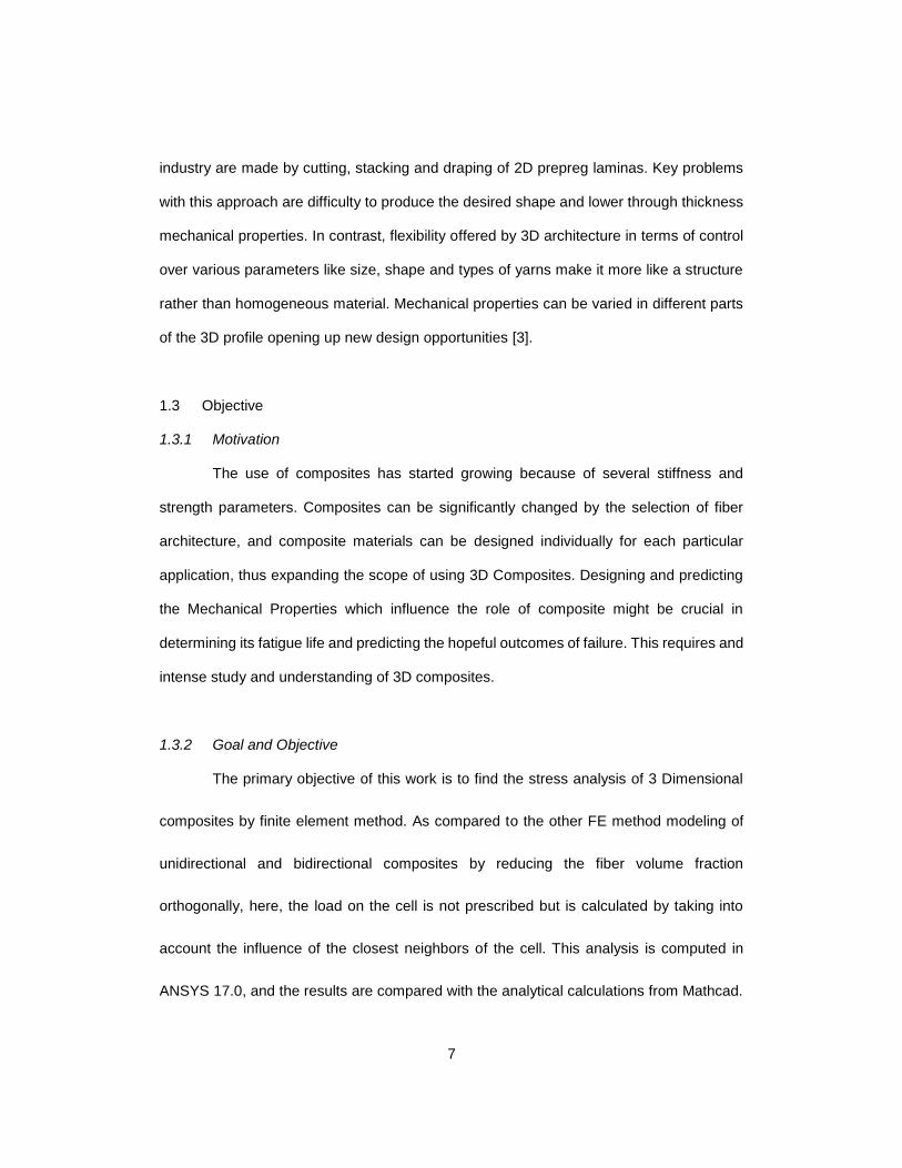
1.2 Need of 3D Composites

Tailoring the alignment of fibers in a composite material or structure is crucial for

maximizing properties like strength, stiffness, fracture toughness, damage resilience and

in order to achieve good multiaxial performance in three dimensions. Three dimensional

(3D) composites are characterized by yarns oriented not only in-plane but also out of plane

resulting in higher through thickness strength and stiffness of the composite material.

Freedom to manipulate cross-sectional size, shape and number of yarns means ‘3D

Architecturing’ makes the design space much bigger. Examples of possible application of

3D composite in this regard are stiffeners and stringers of an aircraft where loads can be

in-plane as well as out of plane. Limited growth of delamination in through thickness

direction results in higher penetration resistance of 3D composites. Also, it has been shown

that velocity corresponding to full penetration is higher for 3D orthogonal woven composite

compared to 2D plane weave composite. Most composite beams used today in aerospace

7

industry are made by cutting, stacking and draping of 2D prepreg laminas. Key problems

with this approach are difficulty to produce the desired shape and lower through thickness

mechanical properties. In contrast, flexibility offered by 3D architecture in terms of control

over various parameters like size, shape and types of yarns make it more like a structure

rather than homogeneous material. Mechanical properties can be varied in different parts

of the 3D profile opening up new design opportunities [3].

1.3 Objective

1.3.1 Motivation

The use of composites has started growing because of several stiffness and

strength parameters. Composites can be significantly changed by the selection of fiber

architecture, and composite materials can be designed individually for each particular

application, thus expanding the scope of using 3D Composites. Designing and predicting

the Mechanical Properties which influence the role of composite might be crucial in

determining its fatigue life and predicting the hopeful outcomes of failure. This requires and

intense study and understanding of 3D composites.

1.3.2 Goal and Objective

The primary objective of this work is to find the stress analysis of 3 Dimensional

composites by finite element method. As compared to the other FE method modeling of

unidirectional and bidirectional composites by reducing the fiber volume fraction

orthogonally, here, the load on the cell is not prescribed but is calculated by taking into

account the influence of the closest neighbors of the cell. This analysis is computed in

ANSYS 17.0, and the results are compared with the analytical calculations from Mathcad.

8

Since the strength along the thickness of the composites is not high, precise prediction of

it is important. It can be done by the detailed study of stress distribution on individual

components of composite material. Independently of boundary conditions at infinity

(applied stresses), the distribution of stresses in the main array is double periodic one.

Finite Element Modeling of a composite material is considered as of to compare

the Effective modulus of 3dimensional cell model as of with the reduced fiber volume

fraction cells in respective directions and also to determine the major difference in behavior

of the respective components of composites materials.

Objective of this thesis can be summarized into

• To Estimate effectiveness of reinforcement in 3rd direction.

• To compare with approximate theoretical models.

• To estimate stress concentration.

9

2 Chapter

LITERATURE REVIEW

Carbon fibre reinforced polymer (CFRP) composites are widely utilized in

aerospace and automotive structures due to their high strength and stiffness to weight

ratios. These long fibre composites are designed to possess high axial stiffness and tensile

strength but the compressive strength of unidirectional composites rarely exceeds 60% of

their tensile strength. The main competing mechanisms governing the compressive

strength of long fibre composites are: (i) elastic micro-buckling (an elastic instability

involving matrix shear); (ii) plastic microbuckling in which the matrix deforms plastically; (iii)

fibre crushing (a compressive fibre failure mode); (iv) splitting by matrix cracking parallel to

the main fibre direction; (v) buckle delamination and (vi) shear band formation at 45o to the

main axis of loading due to matrix yielding [3].

According to Spatially Reinforced Composites Book by I. G. Zhigun, I︠ U︡. M.

Tarnopolʹskiĭ, V. A. Polyakov [10]. In material with a regular picture, it is easy to isolate the

repeating elements in the form of a plane laminae. Disregarding the inhomogeneity of

structure in each lamina and finding out the significant characteristics as those of a quasi-

homogeneous material, the deformation model of material can be represented in the form

of an inhomogeneous block composed of different laminae. The elastic characteristics of

each lamina are determined by the properties of the components and their volume fraction;

construction of the calculation model of material is completed by imposition of laminae on

each other. For this reason, it is necessary to write out the stiffness components for each

lamina in the system of coordinates 1,2,3, turned relative to the initial, in the general case,

non-orthogonal vectors ai = 1, 2, 3, and employ, with the second assumption taken into

10

account, the general formulas that correspond to the joint deformation of a package of

laminae. In modelling of a laminated medium, the macro stresses relate to an individual

lamina, having its own deformation characteristics. The integral averaging of these

stresses throughout the volume of material comprising all the laminae leads to mean

stresses.

Figure 2-1: Composite Structure from Spatially reinforced composite book.

The procedure of calculation of the elastic constants is reduced to the following

stages. Let the reinforcement be represented by a system of three straight threads,

whose direction coincides with three non-coplanar vectors a1, a2, a3 (Figure 2-2). Let us

isolate the plane of a lamina, which passes through vectors a1, a2. Two laminae are

modelled in the material parallel to this plane, containing conditionally only the fibers of

a2, a3 directions and, respectively, a 2, a3 [5].

11

Figure 2-2: 3-Dimensional Thread alignments

The modelling of the laminae for a three-dimensional fibrous material is based on

two assumptions, corresponding to constant density of fiber packing. With bulk

reinforcement coefficient µ1, µ2, µ3 respectively for a1, a2, a3 directions, two laminae, being

parallel to the plane, and passing through a1, a2 vectors, have

1. Identical reinforcement coefficient equal to µ3 (in a3 direction) and µ1 + µ2 (in a3,

direction for the first lamina and a2 for the second lamina)

2. Different relative thicknesses, equal to µ1/ (µ2 + µ3) and µ2/ (µ1 + µ3) respectively.

The elastic characteristics of each lamina are determined by the properties of the

components and their volume fraction; construction of the calculation model of material is

completed by imposition of laminae on each other. For this reason, it is necessary to write

out the stiffness components for each lamina in the system of coordinates 1,2,3, turned

relative to the initial, in the general case, non-orthogonal! vectors ai, i = 1, 2, 3, and employ,

with the second assumption taken into account, the general formulas that correspond to

12

the joint deformation of a package of laminae. In modelling of a laminated medium, the

macro stresses relate to an individual lamina, having its own deformation characteristics.

The integral averaging of these stresses throughout the volume of material comprising all

the laminae leads to mean stresses [5].

For models of material, which will be examined further, the orthogonality of a3

vector to a1 and a2 vectors ((Figure 2-3) is characteristic. This special feature simplifies the

calculation of the characteristics of material and efficient constants of material through

imposition of laminae.

According to Das [3], The tailoring of fiber/tow architectures in CFRPs has also been widely

used to improve properties including the compressive response. The most common

approaches include modifying 2D composites by adding out-of-plane reinforcements. This

is typically achieved by Z-pinning, stitching and knitting More recently, a range of

techniques has been developed to manufacture three-dimensional (3D) fabrics wherein

tows are present in at-least three orthogonal directions; see [15] for a detailed review of

these techniques. In brief, 3D fabrics fall into three categories: (i) 2D woven 3D fabrics

produced by usual 2D weaving methods with monodirectional shedding5; (ii) 3D woven

fabrics produced by a dual-direction shedding system and (iii) non-woven 3D fabrics

without interlacing or interweaving produced by a technique known as “noobing” that is

described in Section 4.2. The ability to manipulate the volume fractions of fiber in three

directions not only allows tailoring of the multi-axial properties of composites; it also

reduces the susceptibility to delamination, which results in an improvement in the impact

performance of CFRPs. Moreover, 3D composites can add more functionality to any

eventual component as discussed by Stig.

13

(Whitney and Riley, 1965-66; Hermans, 1967) did the study on effective elastic moduli

of fiber-reinforced composite. The model they used was concentric cylinder matrix with

cylindrical fiber embedded in it, by considering Reuss and Voigt‘type estimation for elastic

moduli to find out the results. This work was followed by Hashin and Rosen. They used the

model that consisted of fiber embedded in an unbounded solid possessing the effective

moduli of the composite. They were able to formulate the result, but they never explicitly

solved the problem.

14

3 Chapter

MATERIAL CHARACTERISATION

One of the basic requirements to accurately run a model in ANSYS is the materials

and its properties. It is necessary to have all the required material properties to find the

stresses and deformation in a composite material. The properties required to run a model

in ANSYS are:

• Young ‘s modulus

• Poison ‘s ratio

• Density

• Shear modulus

• Coefficient of thermal expansion

Since, composite is made up of two constituents, i.e., matrix and fiber, each of the

constituent can be described with different materials and their respective properties [4].

3.1 MATRIX

A matrix in a composite is a surrounding medium in which fiber is cast or shaped. Its

function is to transfer stresses between the fibers and provide a barrier against adverse

environments. It also protects the surface from abrasion. The matrix materials used in this

work are:

3.1.1 Epoxy

Epoxies are polymerizable thermosetting resins and are available in a variety of

viscosities from liquid to solid. Epoxies are used widely in resins for prepreg materials and

structural adhesives. The processing or curing of epoxies is slower than polyester resins.

Processing techniques include autoclave molding, filament winding, press molding,

vacuum bag molding, resin transfer molding, and pultrusion [4]. Curing temperatures vary

15

from room temperature to approximately 350 °F (180 °C) [16]. The most common cure

temperatures range between 250° and 350°F (120–180 °C). According to L. S. Penn and

T. T. Chiao., when epoxy resin reacts with a curing agent, it does not release any volatiles

or water. Therefore, epoxy does not easily shrink as compared to polyesters or phenolic

resins. Moreover, epoxy resins which are cured provide excellent electrical insulation and

are resistant to chemicals (1982).

Figure 3-1: Epoxy Resin

The advantages of epoxies are high strength and modulus, low levels of volatiles,

excellent adhesion, low shrinkage, good chemical resistance, and ease of processing.

Their major disadvantages are brittleness and the reduction of properties in the presence

of moisture.

16

Density 1.17 gm/cm3

Tensile Strength 80 MPa

Youngs Modulus 3.4 GPa

Poisson’s Ratio 0.36

Table 1: Material Properties of Epoxy Matrix

3.2 FIBER

3.2.1 E Glass

Fibers are used to strengthen the composites; they are the principal constituents

in fiber reinforced composite materials. Fibers carry majority of the load in composites.

They occupy the largest volume fraction of the composite. As the amount of fiber increases

the specific strength of the composite increases, since fibers have low weight density.

Based upon the material characterization, various kinds of fibers are used.

Figure 3-2 : Fiber - E Glass

17

Density 2.54 gm/cm3

Tensile Strength 3.45 GPa

Youngs Modulus 72.4 GPa

Poisson’s Ratio 0.21

Table 2 : Material Properties of E Glass Fiber

18

4 Chapter

MODELLING AND SIMULATION

4.1 Modeling of 3D reinforced composites

This chapter deals with the FEA modeling and simulation techniques used for

unidirectional reinforced composites. The procedure used for the analysis is discussed in

the following steps:

1. Modeling: Create the geometric model according to the required dimensions in

Catia V5.

2. Preprocessing: Import the model from Catia V5 to ANSYS v14.5, define material

properties.

3. Meshing: Creating a refined mesh to provide a better approximation of the solution.

4. Solution process: Applying boundary conditions such as loads and supports to the

body, selecting output control, and obtaining the results.

5. Post processing: Review the obtained results and taking the values, plot the

graphs.

Few assumptions were made during processing of finite element analysis.

• The fibers are cylinders with circular in cross-section.

• The displacements are continuous across the fiber and matrix interface.

• The temperature is uniform, and the material properties do not vary with

temperature.

Normal to the surface and shear stresses are continuous.

19

4.2 GEOMETRY

The Standard Model Discussed in Book Spatially Reinforced Composites Book by

by Ivan Grigorʹevich Zhigun, I︠ U︡. M. Tarnopolʹskiĭ, V. A. and also Considering the work

Described by Satyajit Das [3], The Specimen Model was considered is 3D reinforced

composite comprising E-Glass Fiber (non-twisted E-Glass Fibers) in a epoxy matrix with a

glass transition temperature of 1800 C. The fibers are approximately 𝑑 = 2 mm in diameter

and the 3D composite was anisotropic with 7.8 % of the total number of tows in 𝑍-direction

and 46.07% each in the 𝑋 and 𝑌-directions. Blocks of the 3D reinforced composite of size

9 (𝑋)mm × 9 (𝑌)mm ×9.2 (𝑍)mm were Designed in CAD Software (CATIA V5 R20).

Figure 4-1: Microstructure unit cell Selection from the standard 3D composite structure

20

4.3 VOLUME FRACTION

The composite comprises four principal phases: (i) the 𝑋, 𝑌 and 𝑍-direction Fibers

and (ii) matrix pockets. Based on the unit cell with dimensions sketched in Figure 4-1, the

𝑋 and 𝑌-direction fibers comprise a volume fraction 𝑣𝑋 = 𝑣𝑌 ≈ 22.75% each of the composite

while the 𝑍-direction fiber occupy a volume fraction 𝑣𝑍 ≈ 3.9 % of the composite. The

remainder 𝑣𝑀 = 50.61 % of the volume is occupied by the matrix pockets. It now remains

to specify the overall fiber volume fraction within the composite.

Figure 4-2: Designed 3D Composite Structure

To Compare the 3D Reinforced Model with the reduced Volume Fractions

orthogonally, we have considered the other models which have reduced volume fractions

in respective orthogonal directions as shown in the Figures Below.

21

Figure 4-3 : Reduced Z Fibers(Left) and Reduced Y Fibers (Right).

The Reduced Z Fiber Model (Figure 4-3) Consists of the 𝑋 and 𝑌-direction fibers

comprise a volume fraction 𝑣𝑋 = 𝑣𝑌 ≈ 22.75% each of the composite while the 𝑍-direction

Fiber occupy a volume fraction 𝑣𝑍 = 0 % of the composite. The remainder 𝑣𝑀 ≈ 54.5 % of

the volume is occupied by the matrix pockets. Hence increase in Matrix Volume as of with

3D Reinforced Model.

The Reduced Y Fiber Model (Figure 4-3) Consists of the 𝑋 and 𝑌-direction fibers

comprise a volume fraction 𝑣𝑋 ≈ 22.75% and 𝑣𝑌 = 0% respectively of the composite while

the 𝑍-direction Fiber occupy a volume fraction 𝑣𝑍 ≈ 3.8 % of the composite. The remainder

𝑣𝑀 ≈ 73.3 % of the volume is occupied by the matrix pockets. Hence increase in Matrix

Volume as of with 3D Reinforced Model.

22

Figure 4-4 : Reduced Y & Z Fibers (Left) and Reduced X & Y Fibers(Right)

The Reduced Y and Z Fibers Model (Figure 4-6) Consists of the 𝑋 and 𝑌-direction

fibers comprise a volume fraction 𝑣𝑋 ≈ 22.75% and 𝑣𝑌 = 0% respectively of the composite

while the 𝑍-direction Fiber occupy a volume fraction 𝑣𝑍 = 0% of the composite. The

remainder 𝑣𝑀 ≈ 77.25 % of the volume is occupied by the matrix pockets. Hence increase

in Matrix Volume as of with 3D Reinforced Model.

The Reduced Z Fiber Model (Figure 4-6) Consists of the 𝑋 and 𝑌-direction fibers

comprise a volume fraction 𝑣𝑋 = 𝑣𝑌 =0% each of the composite while the 𝑍-direction Fiber

occupy a volume fraction 𝑣𝑍 ≈ 3.8 % of the composite. The remainder 𝑣𝑀 ≈ 96.2 % of the

volume is occupied by the matrix pockets. Hence increase in Matrix Volume as of with 3D

Reinforced Model.

23

4.4 FINITE ELEMENT/ MESH GENERATION

The goal of meshing in ANSYS Workbench is to provide robust, easy to use meshing

tools that will simplify the mesh generation process. These tools have the benefit of being

highly automated along with having a moderate to high degree of user control.

The required Model is meshed to Refinement till the values converge. The

convergence of the Refinement is judged by noting the results at different locations and

parameters in order to make it consistent and to overcome the singularities which might

affect the study of values which may be crucial in analyzing composite.

Mesh Convergence Report is generated by applying some test loads on the models.

The Table shows the stress report for convergence.

Figure 4-5 : Mesh Convergence plot

-60

-50

-40

-30

-20

-10

0

0 2000000 4000000 6000000 8000000

Stre

ss M

Pa

No of Nodes

Mesh Convergence Plot

1-Stress On XFibers

2-Stress On YFibers

3-Stress On ZFibers

4-Stress BetweenFibers/(-10)

Avg IntegrationMean Stress OnFiber(-ve)

24

1, Similarly for 2 on Y Fibers

4

3

The model was fully meshed in ANSYS with a body sizing of 15μm and face

meshing of size 10μm was done at the interface between matrix and fiber. Since the

stresses calculated are crucial in differentiating the difference between Reduced models,

the meshing has to be fine to obtain more accurate results.

No of Nodes: - 5014494

Min Edge Length: 2.2927e-003 mm

Max Edge Length: 2.9027e-003 mm

Error Ratio: 2.67 %

Figure 4-6 : Locations considered for mesh convergence test

25

Figure 4-7 : Fully Meshed 3D Composite Unit Cell

4.5 ELASTIC PROPERTIES

As discussed in The Stress Analysis Method for Three-Dimensional Composite

Materials by Kanehiro Nagai, Atsushi Yokoyama, Zen'ichiro Maekawa and Hiroyuki

Hamada. We will treat a unit cell volume as 3-D anisotropic space shown in Figure 4-10,

in which material properties would continuously vary in three orthogonal directions and

derive the fundamental formulas for equivalent mechanical properties to this space.

26

Figure 4-8 : Unit cell volume. 3-dimensional anisotropic space

These formulas are deduced for Young's modulus, shear modulus, and Poisson's

ratio. The size of unit cell volume is represented by Lx, Ly, and Lz as shown in Figure 4-10,

and the material properties of an infinitesimal representative volume with edges dx, dy, and

dz at an arbitrary point (x, y, z) in this space are defined.

Where the following Maxwell's Reciprocal Theorem between Young's moduli and Poisson's

ratio is assumed.

In the case of 3-D composite material, each point in this unit cell volume would

corresponds to fiber, resin, void, crack and so on.

4.5.1 Youngs Modulus

To understand the present analytical methodology for Young's modulus, firstly we

will derive the formulas about 2-D area as shown in Figure 4-9. In this region, Young's

moduli in 𝜁 and 𝜂 direction are defined as �̅�𝜍(𝜁) and �̅�𝜂(𝜁) respectively, which are assumed

here to be functions of 𝜁. For the 𝜁 -direction, the relation between the total strain 𝜖𝜍 to this

27

region and the local strain 𝜖(̅𝜁) to an infinitesimal rectangular area with sides 𝑑𝜁 and 𝐿𝜂 at

distance 𝜁 is formed as follows:

……………………………………………….………………….. (1)

As the 𝜁 -directional stress 𝜎𝜍 is independent of 𝜁, the strain �̅�𝜍(𝜁) is

………………………………………………………………………… (2)

Accordingly the 𝜁 -directional total Young's Modulus 𝐸𝜁 (can be obtained from Equations

(5) and (6) as follows:

Figure 4-9 : Explanatory illustration of analytical approach for Young's modulus (2-D).

For the 𝜂 -direction, the relation between the total strain 𝜖𝜂 to this region and the

local stress 𝜎𝜂 ̅̅̅̅ (𝜁) to an infinitesimal area with sides 𝑑𝜁 and 𝐿𝜂 at an arbitrary if, would be

formed as follows:

……………………………………………………………………. (3)

The 𝜂 -directional total stress 𝜎𝜂 is obtained as the following integrated form:

…………………………………………………………………… (4)

28

……………………………………………… (5, from 3 and 4)

Figure 4-10 : Explanatory illustration of analytical approach for Young's modulus (3-D).

Hence the Resulting equation is.

…………………………………… (6)

29

4.5.2 SHEAR MODULUS

Figure 4-11 : Explanatory illustration of analytical approach for Shear modulus (2-D)

To understand the present analytical methodology for the shear modulus, a

formula on 2-D area as shown in Figure 4-11 will be derived. In this region, the shear

modulus �̅�𝜍𝜂(𝜁) is assumed to be a function of 𝜁. The relation between the total shear strain

Υ, and the local shear strain Υ̅(𝜁) for an infinitesimal rectangular area with sides 𝑑𝜁 and 𝐿𝜂

at 𝜁, is given by

………………………………………………………………….. (7)

As the shear stress 𝜏𝜁𝜂 is independent of 𝜁, the following relation is formed.

….……………………………………………………………… (8)

Thus, using Equations (7) and (8), the total shear modulus 𝐺𝜍𝜂 could be expressed as

follows:

…………………………………………………………… (9)

30

Figure 4-12 : Explanatory illustration of analytical approach for Shear modulus (3-D).

Hence Shear Modulus 𝐺𝜍𝜂 is

31

4.6 LOAD SETUP

Knowing that the composite needs to be analyzed with both compressive and shear

loads. It requires a proper load set up. The following Figures shows the Load set for the

desired Composite unit cell.

Figure 4-13 : Compressive Load setup 2D Representation

A displacement of total 10% of the edge length is applied on the either sides of the

composite. Each side is applied a 0.45mm of displacement to form a compressive load.

Then the results are evaluated accordingly to note the changes and post process the

output.

32

Figure 4-14: Compressive Load setup 3D Isometric Representation

Figure 4-15 : Shear Load Setup 2D Representation

A displacement of total 10% of the edge length is applied on one side(A) of the

composite making other end fixed(B). Load acting side is applied a 0.45mm of

33

displacement to form a shear load in the plane. Then the results are evaluated accordingly

to note the changes and post process the output.

Figure 4-16 : Shear Load Setup 3d isometric representation

34

5 Chapter

RESULTS AND DISCUSSION

For finding the force exerted on individual components which can be further used

to find the Effective Modulus, we need a Volume integral Stress value. We can obtain

Integrated Avg Stress value directly from Ansys 14.5 User defined Values feature.

The 3-D integration of Rectangular blocks

Figure 5-1 : 3D Unit Cell

Where, 𝑓(𝑥, 𝑦, 𝑧) = 𝜎(𝑥, 𝑦, 𝑧) The numerical integration of general axisymmetric elements gives:

Where, 𝑓(𝑟, 𝑧, 𝜃) = 𝜎(𝑟, 𝑧, 𝜃)

35

5.1 Tensile Compressive Loads

5.1.1 X Compressive Loads

Figure 5-2 : X Compressive Load Setup (0.45 mm of displacement on each face)

From following figures, Compressive stress(-ve) integral at points concentrate

Maximum at outer bound and minimum occurs at interaction point with other fiber. This

stress is computed by integrating the stress at volumes on X Fibers, and then finding out

the required average value of Stress that can be computed to find total force on the

elements.

To find the Sum of Forces on System

∫ 𝛔(f) 𝑑𝑉(𝑥) + ∫𝛔(𝐦) 𝑑𝑉(𝑦 + 𝑧 + 𝑚)𝑉𝑉

= ∑ 𝐹

Where, ∫ 𝛔(f) 𝑑𝑉(𝑥)𝑉

is normal stress(x) integral along X fibers Volume

And ∫ 𝛔(𝐦) 𝑑𝑉(𝑦 + 𝑧 + 𝑚)𝑉

is normal stress(x) integral along Y Fibers, Z Fibers and Matrix

Volumes

Here, the contribution of Y and Z fibers Stresses are quite less, almost equal to Matrix

stress. Hence, Neglecting the individual contribution of Y and Z fibers and taking whole Y,

Z fibers and Matrix together with Matrix Stresses.

36

To find the Total Stress Induced on System

∑ 𝐹

∑ 𝐴= < 𝜎 >, Where ∑ 𝐴 is the total Cross-sectional area of the Unit Cell.

Therefore, Required Effective Modulus can be found by

< 𝐸 >=< 𝜎 >

< 𝜀 >

Where, Strain < 𝜀 >=𝑑

𝐿, d- Displacement, L- Edge Length.

And the computed Modulus can be compared to find the accuracy by <ERoughly>

<ERoughly> ∶= 𝐸𝑓. 𝐶𝑓𝑥

Where Ef is the Youngs modulus of Fiber and Cfx is the Volume fraction of Fibers in X

Direction.

Figure 5-3: Normal Stress(X) Integral in X Fibers and Matrix (Vf = 49.38%, 3D

Composite)

37

Figure 5-4 :Normal Stress(X) Integral on X Fibers and Matrix (Vf=45.5% Reduced Z

Fibers)

Figure 5-5: Normal Stress(X) Integral on X Fibers and Matrix (Vf=26.63% Reduced Y

Fibers)

Figure 5-6 :Normal Stress(X) Integral on X Fibers and Matrix (Vf=22.75% Reduced Y and

Z Fibers)

38

*All Stress and Modulus values are in MPa

Fiber (Stress)

Matrix (Stress)

Strain€ Sigma F <Stress> <E> <ERoughly> Difference Diff (%)

Vf =49.38 % All Fibers

-6929.1 -285.22 0.1 -148786.92 -1796.94 17969.43 16473.6 1495.81 8.32

Vf =45.5 % Reduced Z

Fibers

-7224.4 -395.54 0.1 -161406.43 -1949.35 19493.53 16473.6 3019.90 15.49

Vf= 26.63% Reduced Y

Fibers

-6899.1 -278.54 0.1 -147794.46 -1784.9 17849.57 16473.6 1375.95 7.71

Vf =22.75% Reduced Y and

Z Fibers

-7227.1 -346.49 0.1 -158320.06 -1912.08 19120.78 16473.6 2647.15 13.84

Table 3: Effective Modulus results for X Compressive Load setup

39

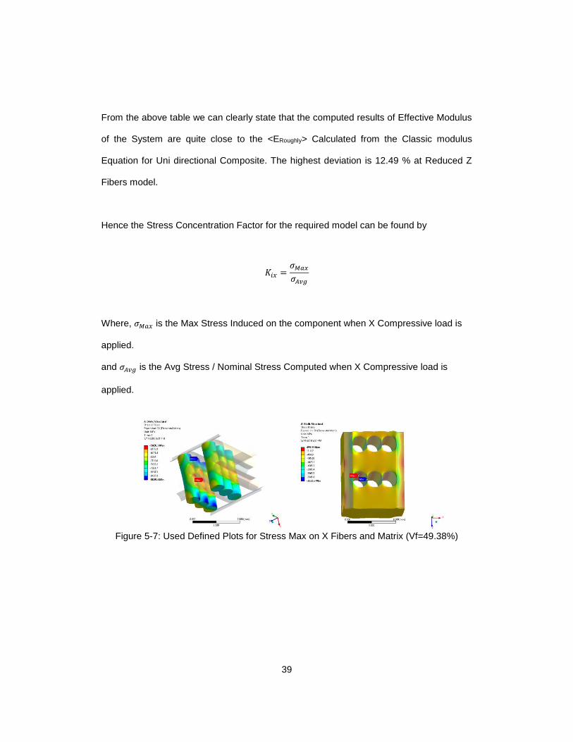
From the above table we can clearly state that the computed results of Effective Modulus

of the System are quite close to the <ERoughly> Calculated from the Classic modulus

Equation for Uni directional Composite. The highest deviation is 12.49 % at Reduced Z

Fibers model.

Hence the Stress Concentration Factor for the required model can be found by

𝐾𝑖𝑥 =𝜎𝑀𝑎𝑥

𝜎𝐴𝑣𝑔

Where, 𝜎𝑀𝑎𝑥 is the Max Stress Induced on the component when X Compressive load is

applied.

and 𝜎𝐴𝑣𝑔 is the Avg Stress / Nominal Stress Computed when X Compressive load is

applied.

Figure 5-7: Used Defined Plots for Stress Max on X Fibers and Matrix (Vf=49.38%)

40

Figure 5-8: User Defined Plots for Stress Max on X Fibers and Matrix (Vf=45.5%

Reduced Z Fibers)


Reduced Y Fibers)


Reduced Y and Z Fibers)

41

Fibers (X Fibers) Matrix

𝜎𝑀𝑎𝑥(𝐹𝑖𝑏𝑒𝑟𝑠) 𝜎𝐴𝑣𝑔(𝐹𝑖𝑏𝑒𝑟𝑠) 𝜎𝑀𝑎𝑥(𝑀𝑎𝑡𝑟𝑖𝑥) 𝜎𝐴𝑣𝑔(𝑀𝑎𝑡𝑟𝑖𝑥) 𝐾𝑓𝑥 𝐾𝑚𝑥


-8819.4 -6929.1 -3825.7 -285.22 1.27 13.41

Vf =45.5 % Reduced Z Fibers

-8954.8 -7224.4 -2989.9 -395.54 1.24 7.56

Vf =26.63% Reduced Y Fibers

-7506.2 -6899.1 -1015.2 -278.54 1.09 3.64

Vf =22.75% Reduced Y and Z

Fibers

-7239.6 -7227.1 -365.59 -346.49 1.00 1.06

* All Stress values are in MPa

Table 4 : Computed Stress Concentration Factors of X Fibers and Matrix when X Compressive Load is applied

42

5.1.2 Y Compressive Load

Figure 5-11: Y Compressive Load Setup (0.45 mm of displacement on each face)

Similarly, Y Compressive Computations on Unit cell are performed as X Compressive

Computations, and then the results are Post processed to obtain effective modulus(<E>)

and stress concentration factor(K).

Figure 5-12: Normal Stress(Y) Integral in Y Fibers and Matrix (Vf = 49.38%, 3D

Composite)

43

Figure 5-13:Normal Stress(Y) Integral on Y Fibers and Matrix (Vf=45.5% Reduced Z

Fibers)

44

Y Compressive

Fiber (Stress)

Matrix (Stress)

Strain€ Sigma F <Stress> <E> E Rough Difference Diff (%)


-6936.1 -309.7 0.1 -148786.92 -1817.45 18174.46 16473.62 1700.838 9.36

Vf =45.5 % Reduced Z

Fibers

-6893.5 -257.94 0.1 -146371.38 -1767.77 17677.7 16473.62 1204.08 6.81

Table 5 : Effective Modulus results for Y Compressive Load setup


45


of the System are quite close to the <ERoughly> Calculated from the Classic modulus

Equation for Uni directional Composite.


𝐾𝑖𝑦 =𝜎𝑀𝑎𝑥

𝜎𝐴𝑣𝑔

Where, 𝜎𝑀𝑎𝑥 is the Max Stress Induced on the component when Y Compressive load is

applied.

and 𝜎𝐴𝑣𝑔 is the Avg Stress / Nominal Stress Computed when Y Compressive load is

applied.

Figure 5-14: Used Defined Plots for Stress Max on Y Fibers and Matrix (Vf=49.38%)

Figure 5-15: User Defined Plots for Stress Max on Y Fibers and Matrix (Vf=45.50%

Reduced Z Fibers)

46

Fibers (Y Fibers) Matrix

𝜎𝑀𝑎𝑥(𝐹𝑖𝑏𝑒𝑟𝑠) 𝜎𝐴𝑣𝑔(𝐹𝑖𝑏𝑒𝑟𝑠) 𝜎𝑀𝑎𝑥(𝑀𝑎𝑡𝑟𝑖𝑥) 𝜎𝐴𝑣𝑔(𝑀𝑎𝑡𝑟𝑖𝑥) 𝐾𝑓𝑦 𝐾𝑚𝑦


-8873.3 -6936.1 -4027.4 -309.7 1.28 13.00

Vf =45.5 % Reduced Z Fibers

-8933.9 -6893.5 -2949.4 -257.94 1.29 11.43

Table 6 : Computed Stress Concentration Factors of Y Fibers and Matrix when Y Compressive Load is applied


47

5.1.3 Z Compressive Load

Figure 5-16: Z Compressive Load Setup (0.45 mm of displacement on each face)

Similarly, Z Compressive Computations on Unit cell are performed as X and Y

Compressive Computations, and then the results are Post processed to obtain effective

modulus(<E>) and stress concentration factor(K).

Figure 5-17:Normal Stress(Z) Integral in Z Fibers and Matrix (Vf = 49.38%, 3D

Composite)

48

Figure 5-18:Normal Stress(Z) Integral on Y Fibers and Matrix (Vf=26.63% Reduced Y

Fibers)

Figure 5-19:Normal Stress(Z) Integral on Y Fibers and Matrix (Vf=3.87% Reduced X and

Y Fibers)

49


Z Compressive Fiber (Stress)

Matrix (Stress)

Strain€ Sigma F <Stress> <E> E Rough Difference Diff (%)

Vf=49.38 % All Fibers

-7084.6 -871.09 0.0978261 -90068.71 -1111.96 11366.7 2806.617 8560.079 75.31

Vf=26.63% (Reduced Y

Fibers)

-7331.9 -253.92 0.0978261 -42792.38 -528.301 5400.41 2806.617 2593.792 48.03

Vf=3.87% (Reduced X

and Y Fibers

-7077.3 -333.04 0.0978261 -48153.22 -594.484 6076.949 2806.617 3270.332 53.82

Table 7 : Effective Modulus results for Z Compressive Load setup

50


of the System possess quite huge difference, this is due to low volume fraction in Z

Direction and the concentration of stress is directly impended on Matrix.


𝐾𝑖𝑧 =𝜎𝑀𝑎𝑥

𝜎𝐴𝑣𝑔

Where, 𝜎𝑀𝑎𝑥 is the Max Stress Induced on the component when Z Compressive load is

applied.

and 𝜎𝐴𝑣𝑔 is the Avg Stress / Nominal Stress Computed when Z Compressive load is

applied.

Figure 5-20: Used Defined Plots for Stress Max on Z Fibers and Matrix (Vf=49.38%)

Figure 5-21: Used Defined Plots for Stress Max on Z Fibers and Matrix (Vf=22.75%

Reduced Y Fibers)

51

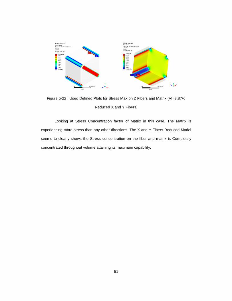
Figure 5-22 : Used Defined Plots for Stress Max on Z Fibers and Matrix (Vf=3.87%

Reduced X and Y Fibers)

Looking at Stress Concentration factor of Matrix in this case, The Matrix is

experiencing more stress than any other directions. The X and Y Fibers Reduced Model

seems to clearly shows the Stress concentration on the fiber and matrix is Completely

concentrated throughout volume attaining its maximum capability.

52

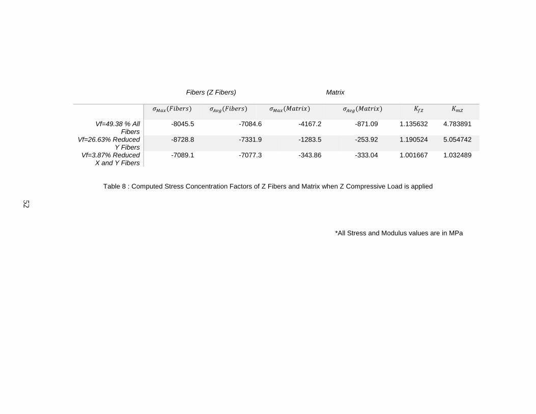
Fibers (Z Fibers) Matrix

𝜎𝑀𝑎𝑥(𝐹𝑖𝑏𝑒𝑟𝑠) 𝜎𝐴𝑣𝑔(𝐹𝑖𝑏𝑒𝑟𝑠) 𝜎𝑀𝑎𝑥(𝑀𝑎𝑡𝑟𝑖𝑥) 𝜎𝐴𝑣𝑔(𝑀𝑎𝑡𝑟𝑖𝑥) 𝐾𝑓𝑍 𝐾𝑚𝑍

Vf=49.38 % All Fibers

-8045.5 -7084.6 -4167.2 -871.09 1.135632 4.783891

Vf=26.63% Reduced Y Fibers

-8728.8 -7331.9 -1283.5 -253.92 1.190524 5.054742

Vf=3.87% Reduced X and Y Fibers

-7089.1 -7077.3 -343.86 -333.04 1.001667 1.032489

Table 8 : Computed Stress Concentration Factors of Z Fibers and Matrix when Z Compressive Load is applied


53

5.2 Shear Loads

5.2.1 X Axis Y Shear (XY Shear)

Figure 5-23: Load Setup for X Axis Y Shear (XY Shear- 0.9 mm Displacement of surface

A)

From following figures, Shear stress integral at points concentrate Maximum at outer bound

and minimum occurs at interaction point with other fiber. This Shear stress is computed by

integrating the stress at volumes on individual components, and then finding out the

required average value of Shear Stress that can be computed to find total force on the

elements.

To find the Sum of Forces on System

∫ 𝛕(fx) 𝑑𝑉(𝑥) + ∫𝛕(fy) 𝑑𝑉(𝑦)𝑉

+ ∫𝛕(fz) 𝑑𝑉(𝑧)𝑉

+ ∫𝛕(𝐦) 𝑑𝑉(𝑚)𝑉𝑉

= ∑ 𝐹

Where, ∫ 𝛕(fx) 𝑑𝑉(𝑥)𝑉

is Shear stress integral along X fibers Volume in acting plane

∫ 𝛕(fy) 𝑑𝑉(𝑦)𝑉

is Shear stress integral along Y fibers Volume in acting plane.

54

∫ 𝛕(fz) 𝑑𝑉(𝑍)𝑉

is Shear stress integral along Z fibers Volume in acting plane

And ∫ 𝛕(𝐦) 𝑑𝑉(𝑚)𝑉

is Shear stress integral along Matrix Volume in acting plane

To find the Total Stress Induced on System

∑ 𝐹

∑ 𝑉= < 𝛕 >, Where ∑ 𝑉 is the total Volume of the Unit Cell.

Formulae used for estimation of the effective properties of 3D composites

1. Recalculation of the properties of fiber (isotropic) and matrix

( )

;3(1 )

;2 1

bulk modulus

shear modulus

EK

EG

=−

=+

2. Shear modulus of modified matrix

( )23

23

4 (1 ) 1;

1(1 )

F M M

M

F M

M M

c G GG G

Gc c

G

c

⊥

⊥

⊥ ⊥

⊥

− −= +

+ + −

− is the volume concentration of all fibers perpendicular to the shear plane

3. Effective shear modulus in the plane

( )2

1 (1 )

F M

F

M

c G GG G

Gc c

G

c

⊥

−= +

+ + −

− is the total volume concentration of all fibers in the plane of shear or parallel to it

After applying load on the unit cell, the following plots have been noted for Avg Shear

Stress in XY Plane.

55

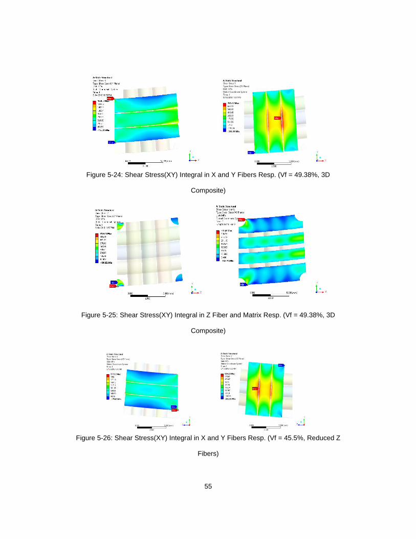
Figure 5-24: Shear Stress(XY) Integral in X and Y Fibers Resp. (Vf = 49.38%, 3D

Composite)

Figure 5-25: Shear Stress(XY) Integral in Z Fiber and Matrix Resp. (Vf = 49.38%, 3D

Composite)

Figure 5-26: Shear Stress(XY) Integral in X and Y Fibers Resp. (Vf = 45.5%, Reduced Z

Fibers)

56

Figure 5-27: Shear Stress (XY) Integral in Matrix (Vf=45.5%, Reduced Z Fibers)

Figure 5-28: Shear Stress (XY) Integral in X and Z Fibers Resp. (Vf=26.63%, Reduced Y

Fibers)

Figure 5-29: Shear Stress (XY) Integral in Matrix. (Vf=26.63%, Reduced Y Fibers)

57

Figure 5-30: Shear Stress (XY) Integral in X Fibers and Matrix Resp. (Vf=22.75%,

Reduced Y and Z Fibers)

Figure 5-31: Shear Stress (XY) Integral in Z Fibers and Matrix Resp. (Vf=3.87%,

Reduced X and Y Fibers)

58

X axis Y

Shear 𝛕𝑥 Avg 𝛕𝑌

Avg 𝛕𝑍

Avg 𝛕𝑀

Avg ∑ 𝐹 𝜀,

Strain 𝛕

<G> 𝐺⊥ 𝐺∥ Difference Difference %

Vf =49.38 % All

Fibers

792.975 433.11 226.48 62.902 238163.7 0.1 319.597 3195.97 1250.07 3049.881 146.0891 4.57

Vf=45.5 % Reduced Z

Fibers

505.94 233.29 0 52.939 146841.3 0.1 197.0495 1970.495 1250 2060.992 -90.4967 -4.59

Vf=26.63% Reduced Y

Fibers

515.27 0 155.21 119.96 157441.3 0.1 211.2738 2112.738 1250.07 1911.811 200.9269 9.51

Vf=22.75% Reduced Y

and Z Fibers

511.07 0 0 93.492 140474.8 0.1 188.5061 1885.061 1250 1911.709 -26.6475 -1.41

Vf=3.87% Reduced X

and Y Fibers

0 0 219.7 113.566 87695.38 0.1 117.6803 1176.803 1250.07 1250.07 -73.2664 -6.23

Table 9 :Effective Shear Modulus results for X Y Shear Load setup


59


𝐾𝑖 =𝜏𝑀𝑎𝑥

𝜏𝐴𝑣𝑔

Where, 𝜏𝑀𝑎𝑥 is the Max Stress Induced on the component when XY Shear load is

applied.

and 𝜏𝐴𝑣𝑔 is the Avg Stress / Nominal Stress Computed when XY Shear load is applied.

60

X axis Y Shear 𝜏𝑥 Max 𝜏𝑌 Max

𝜏𝑍 Max

𝜏𝑀 Max

𝜏𝑥 Avg 𝜏𝑌 Avg

𝜏𝑍 Avg

𝜏𝑀 Avg

Kfx 𝐾𝑓y 𝐾𝑓z 𝐾𝑚


1169.1 703.43 687.17 1250.6 792.97 433.11 226.48 62.902 1.47 1.62 3.03 19.88

Vf=45.5 % Reduced Z

Fibers

1139.3 615.17 0 1061.7 505.94 233.29 0 52.939 2.25 2.64 0 20.05

Vf=26.63% Reduced Y

Fibers

1031.5 0 392.77 1112.6 515.27 0 155.21 119.96 2.00 0 2.53 9.27

Vf=22.75% Reduced Y and

Z Fibers

985.75 0 0 1057.8 511.07 0 0 93.492 1.93 0 0 11.31

Vf=3.87% Reduced X and

Y Fibers

0 0 304.68 138.52 0 0 219.7 113.566 0 0 1.39 1.22

Table 10 : Computed Stress Concentration Factors of Fibers and Matrix when X Y Shear Load is applied


61

Similarly, the procedure is followed for all the shear loads in Different planes.

Hence the Results Follows.

5.2.2 X Axis Z Shear (XZ Shear)

X axis Z Shear 𝛕𝑥 Avg

𝛕𝑌 Avg

𝛕𝑍 Avg

𝛕𝑀 Avg

∑ 𝐹 𝜀, Strain

𝛕

<G> 𝐺⊥ 𝐺∥ Difference Difference %


370.33 306.75 201.76 127.40 168688.39 0.10 226.37 2263.67 1250.50 2061.79 201.88 8.92

Vf=45.5 % Reduced Z Fibers

378.65 319.39 0.00 127.70 170216.08 0.10 228.42 2284.17 1250.50 1912.45 371.72 16.27


448.36 0.00 260.52 100.31 138394.52 0.10 185.71 1857.15 1250.00 2060.99 -203.85 -10.98

Vf=22.75% Reduced Y and Z Fibers

449.82 0.00 0.00 100.01 133841.24 0.10 179.60 1796.04 1250.00 1911.71 -115.66 -6.44


0.00 0.00 219.84 133.88 102252.02 0.10 137.21 1372.14 1250.00 1342.44 29.71 2.16

Table 11 :Effective Shear Modulus results for X Z Shear Load setup


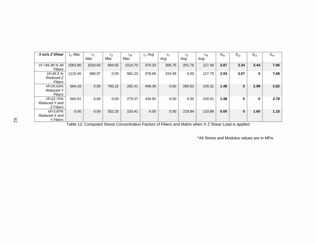
62

X axis Z Shear 𝜏𝑥 Max 𝜏𝑌 Max

𝜏𝑍 Max

𝜏𝑀 Max


𝜏𝑍 Avg

𝜏𝑀 Avg



1062.90 1024.60 694.65 1014.70 370.33 306.75 201.76 127.40 2.87 3.34 3.44 7.96

Vf=45.5 % Reduced Z

Fibers

1110.40 980.97 0.00 981.23 378.65 319.39 0.00 127.70 2.93 3.07 0 7.68

Vf=26.63% Reduced Y

Fibers

664.16 0.00 780.22 282.41 448.36 0.00 260.52 100.31 1.48 0 2.99 2.82


Z Fibers

665.61 0.00 0.00 279.07 449.82 0.00 0.00 100.01 1.48 0 0 2.79


Y Fibers

0.00 0.00 352.20 153.41 0.00 0.00 219.84 133.88 0.00 0 1.60 1.15

Table 12: Computed Stress Concentration Factors of Fibers and Matrix when X Z Shear Load is applied


63

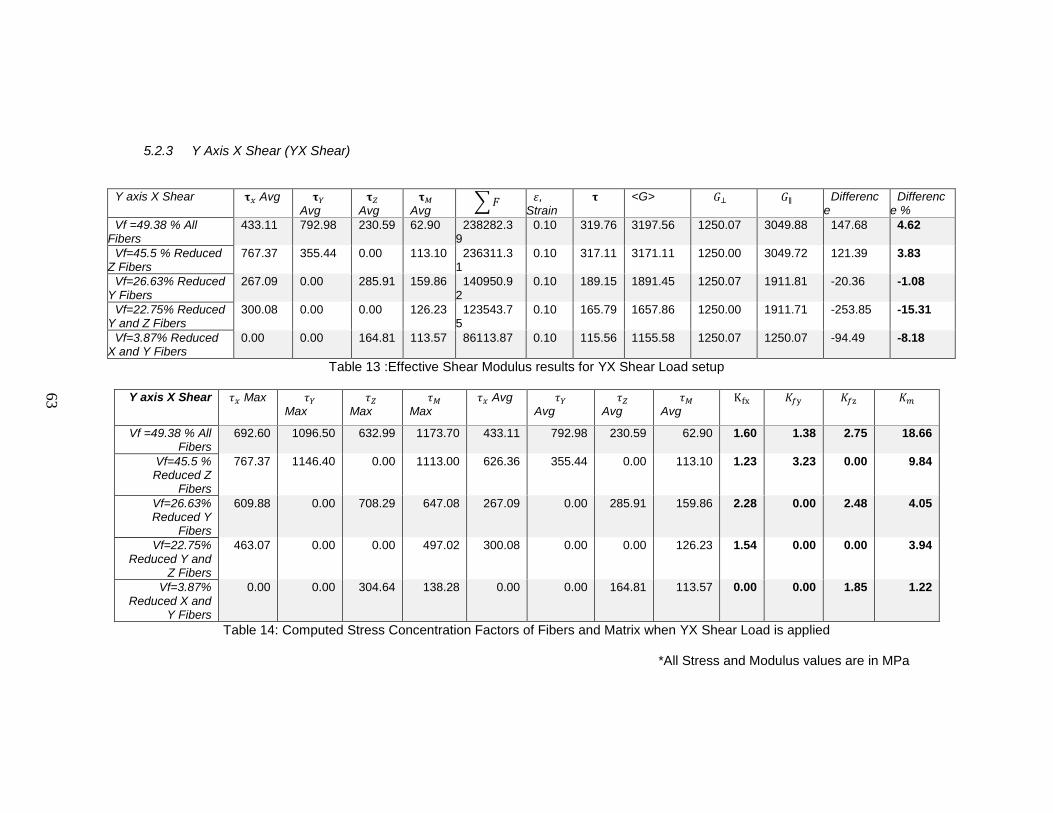
5.2.3 Y Axis X Shear (YX Shear)

Y axis X Shear 𝛕𝑥 Avg 𝛕𝑌

Avg 𝛕𝑍

Avg 𝛕𝑀

Avg ∑ 𝐹 𝜀,

Strain 𝛕

<G> 𝐺⊥ 𝐺∥ Difference

Difference %


433.11 792.98 230.59 62.90 238282.39

0.10 319.76 3197.56 1250.07 3049.88 147.68 4.62


767.37 355.44 0.00 113.10 236311.31

0.10 317.11 3171.11 1250.00 3049.72 121.39 3.83


267.09 0.00 285.91 159.86 140950.92

0.10 189.15 1891.45 1250.07 1911.81 -20.36 -1.08


300.08 0.00 0.00 126.23 123543.75

0.10 165.79 1657.86 1250.00 1911.71 -253.85 -15.31


0.00 0.00 164.81 113.57 86113.87 0.10 115.56 1155.58 1250.07 1250.07 -94.49 -8.18

Table 13 :Effective Shear Modulus results for YX Shear Load setup

Y axis X Shear 𝜏𝑥 Max 𝜏𝑌 Max

𝜏𝑍 Max

𝜏𝑀 Max


𝜏𝑍 Avg

𝜏𝑀 Avg



692.60 1096.50 632.99 1173.70 433.11 792.98 230.59 62.90 1.60 1.38 2.75 18.66

Vf=45.5 % Reduced Z

Fibers

767.37 1146.40 0.00 1113.00 626.36 355.44 0.00 113.10 1.23 3.23 0.00 9.84

Vf=26.63% Reduced Y

Fibers

609.88 0.00 708.29 647.08 267.09 0.00 285.91 159.86 2.28 0.00 2.48 4.05


Z Fibers

463.07 0.00 0.00 497.02 300.08 0.00 0.00 126.23 1.54 0.00 0.00 3.94


Y Fibers

0.00 0.00 304.64 138.28 0.00 0.00 164.81 113.57 0.00 0.00 1.85 1.22

Table 14: Computed Stress Concentration Factors of Fibers and Matrix when YX Shear Load is applied


64

5.2.4 Y Axis Z Shear (YZ Shear)

Y axis Z Shear 𝛕𝑥 Avg 𝛕𝑌

Avg 𝛕𝑍

Avg 𝛕𝑀

Avg ∑ 𝐹 𝜀,

Strain 𝛕


Difference %


322.29 380.95 196.57

127.92 173170.29

0.10 232.38 2323.81 1250.50 2061.79 262.02 11.28


304.29 368.61 0.00 127.16 165734.06

0.10 222.40 2224.02 1250.50 1912.45 311.57 14.01


243.44 0.00 350.26

133.10 124170.03

0.10 166.63 1666.26 1250.50 1912.45 -246.19 -14.77


191.87 0.00 0.00 133.22 109218.75

0.10 146.56 1465.63 1250.50 1250.50 215.13 14.68


0.00 0.00 214.52

111.42 86007.32 0.10 115.42 1154.15 1250.00 1342.44 -188.28 -16.31

Table 15 :Effective Shear Modulus results for YZ Shear Load setup

Y axis Z Shear 𝜏𝑥 Max 𝜏𝑌 Max

𝜏𝑍 Max

𝜏𝑀 Max


𝜏𝑍 Avg

𝜏𝑀 Avg



996.67 1082.90 724.60 1003.00 322.29 380.95 196.57 127.92 3.09 2.84 3.69 7.84

Vf=45.5 % Reduced Z

Fibers

999.77 1085.40 0.00 993.48 304.29 368.61 0.00 127.16 3.29 2.94 0.00 7.81

Vf=26.63% Reduced Y

Fibers

294.31 0.00 766.94 327.03 243.44 0.00 350.26 133.10 1.21 0.00 2.19 2.46


Z Fibers

228.30 0.00 0.00 227.62 191.87 0.00 0.00 133.22 1.19 0.00 0.00 1.71


Y Fibers

0.00 0.00 352.16 153.75 0.00 0.00 214.52 111.42 0.00 0.00 1.64 1.38

Table 16 : Computed Stress Concentration Factors of Fibers and Matrix when YZ Shear Load is applied


65

5.2.5 Z Axis X Shear (ZX Shear)

Z axis X Shear 𝛕𝑥 Avg 𝛕𝑌 Avg

𝛕𝑍 Avg

𝛕𝑀 Avg


𝛕


Difference %


280.43 223.25 154.00

112.31 132214.32

0.10 177.42 1813.64 1250.50 2061.79 -248.15 -13.68


214.38 224.46 0.00 113.47 120487.61

0.10 161.68 1652.78 1250.50 1912.45 -259.67 -15.71


239.88 0.00 229.64

209.24 161710.28

0.10 217.00 2218.25 1250.00 2060.99 157.26 7.09


217.06 0.00 0.00 184.76 143159.94

0.10 192.11 1963.79 1250.00 1911.71 52.08 2.65


0.00 0.00 179.96

154.16 115621.62

0.10 155.16 1586.03 1250.00 1342.44 243.59 15.36

Table 17 :Effective Shear Modulus results for Z X Shear Load setup

Z axis X Shear 𝜏𝑥 Max 𝜏𝑌

Max 𝜏𝑍

Max 𝜏𝑀

Max 𝜏𝑥 Avg 𝜏𝑌

Avg 𝜏𝑍

Avg 𝜏𝑀

Avg Kfx 𝐾𝑓y 𝐾𝑓z 𝐾𝑚


510.59 625.43 922.23 658.59 280.43 223.25 154.00 112.31 1.82 2.80 5.99 5.86

Vf=45.5 % Reduced Z

Fibers

471.76 575.56 0.00 599.61 214.38 224.46 0.00 113.47 2.20 2.56 0.00 5.28

Vf=26.63% Reduced Y

Fibers

383.30 0.00 571.21 320.70 239.88 0.00 229.64 209.24 1.60 0.00 2.49 1.53


Z Fibers

261.24 0.00 0.00 229.36 217.06 0.00 0.00 184.76 1.20 0.00 0.00 1.24


Y Fibers

0.00 0.00 612.93 180.43 0.00 0.00 179.96 154.16 0.00 0.00 3.41 1.17

Table 18: Computed Stress Concentration Factors of Fibers and Matrix when ZX Shear Load is applied


66

5.2.6 Z Axis Y Shear (ZY Shear)

Z axis Y Shear 𝛕𝑥 Avg 𝛕𝑌 Avg

𝛕𝑍 Avg

𝛕𝑀 Avg


𝛕


Difference %


274.43 206.38 166.48 119.57 131435.42

0.10 176.38 1802.95 1250.50 2061.79 -258.83 -14.36


316.92 357.89 0.00 94.61 152837.95

0.10 205.10 2096.54 1250.50 1912.45 184.09 8.78


227.04 0.00 263.08 131.95 118238.50

0.10 158.67 1621.93 1250.50 1463.26 158.67 9.78


202.22 0.00 0.00 112.69 99156.14 0.10 133.06 1360.17 1250.50 1250.50 109.66 8.06


0.00 0.00 179.82 154.16 115617.72

0.10 155.15 1585.98 1250.00 1342.44 243.54 15.36

Table 19:Effective Shear Modulus results for Z Y Shear Load setup

Z axis Y Shear 𝜏𝑥 Max 𝜏𝑌 Max

𝜏𝑍 Max

𝜏𝑀 Max


𝜏𝑍 Avg

𝜏𝑀 Avg



324.17 206.38 207.98 180.04 274.43 140.89 166.48 119.57 1.18 1.46 1.25 1.51

Vf=45.5 % Reduced Z

Fibers

521.29 456.55 0.00 560.32 316.92 357.89 0.00 94.61 1.64 1.28 0.00 5.92

Vf=26.63% Reduced Y

Fibers

349.43 0.00 626.05 399.42 227.04 0.00 263.08 131.95 1.54 0.00 2.38 3.03


Z Fibers

208.99 0.00 0.00 231.16 202.22 0.00 0.00 112.69 1.03 0.00 0.00 2.05


Y Fibers

0.00 0.00 613.01 180.42 0.00 0.00 179.82 154.16 0.00 0.00 3.41 1.17

Table 20: Computed Stress Concentration Factors of Fibers and Matrix when Z Y Shear Load is applied


67

6 Chapter

RESULTS AND CONCLUSION

6.1 Discussion of the results

Prediction of the 𝑋&Y-direction compressive response is included in Section 5.1.1

and Section 5.1.2 with deformed configurations shown in Figures mentioned in Sections at

applied load setups. The FE prediction of the Effective Modulus versus approximate

theoretical modulus response is in reasonable agreement with the measurements except

for the fact that the FE calculations over-predict the peak strength. This is because no initial

imperfection is included in these FE calculations since the 𝑋-direction fibers are not

explicitly modelled. Consistent with observations no significant localised deformation is

observed prior to the peak stress though the FE calculations .The Stress Concentration

Factor of Matrix is observed to be reduced more than ten times from 13.41 in 3D Model to

1.06 in reduced unidirectional model (Table 4 & 6). This reduction clearly states the

response from low fiber volume fraction in the structure.

Prediction of the Z-direction compressive response is included in Section 5.1.3 with

deformed configurations shown in Section 5.1.3 at applied load setup. The FE Prediction

of the effective modulus versus approximate theoretical modulus has comparatively huge

variation due non-considering the role of horizontal fibers contribution (X&Y Fibers) which

take up most of the cross section along Z Direction. But clearly the Stress concentration

factor shows us the response of change in volume fractions by making the matrix

concentrated with peak stresses throughout in Reduced models unlike to the 3d model.

In Case of Shear forces the Effective modulus computed by FE simulations where

having reasonable variations as compared to the derived theoretical modulus Max

difference being around 16%. The Stress concentration factor of the whole models were

68

reasonable with Maximum stress concentration factor being for the 3d Model as of with the

reduced models. The reduced models bare a concentrated stress throughout volume due

to low fiber volume fraction.

6.2 Future Wok

• Overall Structure failure prediction can be performed in order to understand the

growth rate and the fatigue life of the composite model.

• The Ultimate Tensile Strength of the model can be computed to compare the

results with reduced model.

• Considering the popularity of braided materials, this study can be performed on

Considered 3D Braided Composite material.

• Effect of Matrix/Fiber debonding can be studied by applying tensile loading in

transversal direction.

• Stress analysis of composites under thermal loading can be performed.

69

References

[1] H.B. Vinay, H.K. Govindaraju and Prashanth Banker- “A Review on Investigation on the

Influence of Reinforcement on Mechanical Properties of Hybrid Composites”.

[2] Huiyu Sun, Shenglin Di, Nong Zhang, Changchun Wu- “Micromechanics of composite

materials using multivariable finite element method and homogenization theory”.

[3] Satyajit Das- “Mechanics of 3D Composites”.

[4] Pavan Agrawal- “Finite element modeling and stress distribution of unidirectional

composite materials under transversal”.

[5] Kanehiro Nagai, Atsushi Yokoyama, Zen'ichiro Maekawa and Hiroyuki Hamada “The

Stress Analysis Method for Three-Dimensional Composite Materials”.

[6] Lotfi Toubal, Moussa Karama, Bernard Lorrian “Stress Concentration in a Circular hole

in composite plate”.

[7] Wooseok P. Ji and Anthony M. Waas “A Predictive Model for the Compressive Strength

of 3D Woven Textile Composites”.

[8] Christensen, R. M. (2012). Mechanics of composite materials. Courier Corporation.

[9] Van Fo Fy, G. A., Karpinos, D. M., & Tuchinskaya, L. I. (1970). Composite Materials of

Fibrous Structure.

[10] I. G. Zhigun, I︠ U︡. M. Tarnopolʹskiĭ, V. A. Polyakov. “Spatially Reinforced Composites”

Book.

70

BIOGRAPHICAL STATEMENT

Chandra Bhaskar Reddy Pittu received his bachelor’s degree in Aeronautical

Engineering from Jawaharlal Nehru Technological University, Hyderabad in the year 2015.

He then decided to pursue his masters in mechanical engineering from the University of

Texas at Arlington, USA in Fall 2016 and received his degree in Spring 2018.

Master’s Degree provided him a comprehensive background in Mechanical

Technology and kept him abreast of the latest evolutions in this area. In four years of study

of this science, subjects like Finite Element, Additive Manufacturing, Composites, and Fluid

Dynamics dragged his interest. Of all the courses, Computer aided design (CAD) has

evoked a particular stake in him. As a result, he got certified by Dassault systems as

“CATIA V5R20 Part Design Specialist”. Not only Catia, He have also learned other

CAD/CAE software’s like AutoCAD, ANSYS and Solidworks.

He did Internships at National Aerospace laboratories and Boeing when he was

pursuing his Bachelors in Hyderabad. He also published his work on Micro Aerial vehicles

in International Journals on Science and Technology(IJST).

Coming from a business background, Chandra was always ambitious to be an

entrepreneur and start his industry in the field of mechanical engineering. Chandra would

like to use his skills and experience to develop technology for the comfort of humankind by

keeping environmental factors in mind.

Documents

INVESTIGATION ON EFFECTIVE MODULUS AND STRESS