Embed Size (px)
Citation preview

University of Southern Queensland
Faculty of Health, Engineering and Sciences
INVESTIGATION OF SEEPAGE IN WATER SUPPLY
DISTRIBUTION CHANNELS IN ST GEORGE,
QUEENSLAND
A dissertation submitted by
Melissa A. McLean (Fairley)
in fulfilment of the requirements of
Courses ENG4111 and ENG4112 Research Project
towards the degree of
Bachelor of Engineering
Submitted: 29 October 2015

i
Abstract
Keywords: Seepage, Evaporation, Irrigation, Channel, Distribution, Losses, Semi-arid
The annual loss of water in agricultural storage and supply channels due to evaporation
and seepage is estimated to exceed several thousand gigalitres representing billions of
dollars lost to the Australian economy. There is a need for water-saving measures and a
structured approach to assess water loss in earthen supply channels.
The focus of this study (the St George Irrigation Area) [GDA94 S 28.048953°, E
148.582.746°] is the only public dam supplemented agricultural water supply system in
southwest Queensland supplied by earthen channels and it is a major contributor to the
fibre (mainly cotton lint) produced in Australia.
This study measured the seepages losses in 9 km of a 50 year old agricultural channel
water supply system constructed in St George, Queensland. The results of the study
were compared to the seepage losses measured in other Australian studies. The expected
seepage loss was less than 0.035 md-1
.
The ponding test method was used to calculate the daily seepage losses through the bed
and walls of the channel supply system at three sites. The sites were selected based on
soil types and the nature of the use. Absolute pressure sensors installed in three isolated
channel sections measured the rate of drop of the free water surface in the channel. The
daily seepage loss rate was calculated by subtracting the daily evaporation from the rate
of drop of the free water surface.
The estimated seepage loss during May 2015 at Site 3: Buckinbah B2/2 Channel
(designed capacity of 29 MLd-1
) was 0.008 md-1
± 0.002 m (95%).

ii
Certification
I certify that the ideas and experimental work, results, analyses and conclusions set out
in this dissertation are entirely my own effort, except where otherwise indicated and
acknowledged.
I further certify that the work is original and has not been previously submitted for
assessment in any other course or institution, except where specifically stated.
Melissa A. McLean (Fairley)
Student Number: 0019822581

iii
University of Southern Queensland
Faculty of Health, Engineering and Sciences
ENG4111/ENG4112 Research Project
Limitations of Use
The Council of the University of Southern Queensland, its Faculty of Health,
Engineering & Sciences, and the staff of the University of Southern Queensland, do not
accept any responsibility for the truth, accuracy or completeness of material contained
within or associated with this dissertation.
Persons using all or any part of this material do so at their own risk, and not at the risk
of the Council of the University of Southern Queensland, its Faculty of Health,
Engineering & Sciences or the University of Southern Queensland.
This dissertation reports an educational exercise and has no purpose or validity beyond
this exercise. The sole purpose of the course pair entitled “Research Project” is to
contribute to the overall education within the student’s chosen degree program. This
document, the associated hardware, software, drawings, and other material set out in the
associated appendices should not be used for any other purpose: if they are so used, it is
entirely at the risk of the user.

iv
Acknowledgements
The resources and information contributed in this study were provided in part by my
employer the DNRM. I would like to acknowledge the time and assistance offered by
Craig Johansen, DSITI; Justin Schultz, SunWater; my DNRM colleagues Ross Krebs
(decd), Jim Weller, John Ritchie, Sarah Rossiter and my faculty supervisor Malcolm
Gillies, NCEA.
I would like to acknowledge the foundation support that my parents, Evan and Julie
have given to me so that I can complete my tertiary studies and to my father in law,
Greg for helping me fabricate the site installations.
Finally, I would like to acknowledge my husband James, and the patience he has shared
with me during my part-time study and I acknowledge that without his support this
work would not have been realised.

v
Table of Contents
Abstract .............................................................................................................................. i
Certification....................................................................................................................... ii
Limitations of Use ............................................................................................................ iii
Acknowledgements .......................................................................................................... iv
List of Figures ................................................................................................................ viii
List of Tables.................................................................................................................... xi
List of Photographs ......................................................................................................... xii
List of Equations ............................................................................................................ xiii
List of Abbreviations and Units ..................................................................................... xiv
Chapter 1 Introduction ................................................................................................. 1
1.1 Need for the study (The Problem) ...................................................................... 1
1.2 Study objective ................................................................................................... 3
1.3 The use of seepage loss estimates ...................................................................... 4
1.4 Research question ............................................................................................... 6
1.5 Objectives of the study ....................................................................................... 6
Chapter 2 Literature review ......................................................................................... 7
2.1 Background ........................................................................................................ 7
2.1.1 The study area ............................................................................................. 7
2.1.2 Key issues facing the St George district ................................................... 16
2.2 Water distribution losses in channel distribution systems ................................ 18
2.2.1 Australian seepage loss studies ................................................................. 19
2.2.2 Other seepage loss studies outside of Australia ........................................ 21
2.3 Methods to measure seepage losses ................................................................. 21
2.3.1 The Idaho Seepage Meter.......................................................................... 21
2.3.2 Ponding tests ............................................................................................. 22
2.3.3 Inflow-outflow tests .................................................................................. 24
2.3.4 Geophysical methods ................................................................................ 24
vi
2.3.5 Summary of testing methods and method selected for the study .............. 25
2.4 Methods to reduce seepage loss ....................................................................... 26
2.5 Conclusion ........................................................................................................ 28
Chapter 3 Experimental techniques and equipment .................................................. 30
3.1 Introduction ...................................................................................................... 30
3.2 Measurement sites ............................................................................................ 30
3.2.1 Site 1: St George Main Channel ............................................................... 33
3.2.2 Site2: Buckinbah B2 Channel and Site 3: Buckinbah B2/2 Channel........ 35
3.3 Instruments used for the field measurements ................................................... 38
3.3.1 Selection of field instruments.................................................................... 41
3.4 Seepage calculation .......................................................................................... 46
3.4.1 Channel geometry used to estimate the volumetric losses ........................ 46
3.4.2 Monitoring parameters during the test ...................................................... 46
3.4.3 Seepage equations used to analyse the water level field measurements ... 47
3.5 Conclusion ........................................................................................................ 48
Chapter 4 Experimental results and discussion ......................................................... 50
4.1 Experimental measurement .............................................................................. 50
4.2 Water head data ................................................................................................ 51
4.2.1 Site 3: Sample data during normal channel operation .............................. 53
4.2.2 Site 3: Sample data during channel shutdown .......................................... 54
4.3 Fluctuations in the water depth data ................................................................. 56
4.3.1 Instrument error ......................................................................................... 56
4.3.2 Barometric compensation calculation ....................................................... 58
4.3.3 Random error ............................................................................................ 61
4.4 Evapotranspiration and rainfall data ................................................................. 62
4.4.1 Evapotranspiration data compared to evaporation data ............................ 62
4.4.2 Rainfall data .............................................................................................. 65
4.5 Results .............................................................................................................. 66
vii
4.5.1 Site 1: St George Main Channel ............................................................... 66
4.5.2 Site 2: Buckinbah B2 Channel .................................................................. 70
4.5.3 Site 3: Buckinbah B2/2 Channel ............................................................... 72
4.6 Conclusion and review of results ..................................................................... 76
Chapter 5 Conclusion ................................................................................................ 79
5.1 Further work and recommendations ................................................................. 81
References ....................................................................................................................... 83
Appendix A ..................................................................................................................... 86
Appendix B ..................................................................................................................... 85
Appendix C ..................................................................................................................... 94
Appendix D ..................................................................................................................... 98
Appendix E ................................................................................................................... 100
viii
List of Figures
Figure 1.1. Vertical seepage is more likely to be governed by soil conditions (SKM,
2003). ................................................................................................................................ 1
Figure 1.2. St George is located within the Murray-Darling Basin (MDBA, 2015)........ 3
Figure 1.3. Map of the Darling Downs – Maranoa Statistical Region (Queensland
Treasury, 2015). ................................................................................................................ 5
Figure 2.1. The plan area for the Condamine and Balonne catchments (Queensland
Government, 2015). .......................................................................................................... 9
Figure 2.2. St George Irrigation Area Locality Map (GHD, 2001). ............................... 12
Figure 2.3. SGIA Schematic Layout (GHD, 2001). ........................................................ 13
Figure 2.4. A mechanical dethridge wheel is a highly reliable method of water
measurement but has a lower accuracy than modern ultrasonic meters. ........................ 15
Figure 2.5. Idaho Seepage Meter used for point measurement of water
infiltration/seepage (ANCID, 2004b). ............................................................................ 22
Figure 2.6. Seepage rates for typical linings (Sonnichsen, 1993). .................................. 27
Figure 3.1. Site 1 was located on the St George Main Channel (GDA94 S 28.058725° E
148.577346°) to the east of Beeson Road (Google Earth, 2015). ................................... 31
Figure 3.2. Site 2 and Site 3 were located east of the intersection between McDonald
Road and Carnarvon Highway on the Buckinbah B2 Channel (GDA94 S 28.168073° E
148.726985°) and Buckinbah B2/2 Channel offtakes (GDA94 S 28.168295° E
148.727715°); respectively (Google Earth, 2015). ......................................................... 32
Figure 3.3. The measurement sites were located in trapezoidal channels (Irrigation and
Water Supply Commission Queensland, 1972a). ........................................................... 32
Figure 3.4. The typical remnant vegetation cover on a sodosol shown here in profile is
the tall poplar box woodland (CSIRO, 2013a)................................................................ 34
Figure 3.5. The gilgaied landscape shown on the right of the Vertosol profile originally
supported an open forest of brigalow (CSIRO, 2013b). ................................................. 36
Figure 3.6. Components of pondage test water balance per Eqn. 2 (SKM, 2003). ......... 48

ix
Figure 4.1. The seepage losses were estimated using data that suggested the falling
water depth was due to seepage alone............................................................................. 50
Figure 4.2. The time series pressure data and water depth data at Site 3 [April 2015]. . 52
Figure 4.3. The time series pressure data and water depth data at Site 3 [May 2015]. ... 53
Figure 4.4. The time series data and water depth data at Site 3 [11 April 2015]. ........... 54
Figure 4.5. The time series pressure data and water depth data at Site 3 [25 May 2015].
......................................................................................................................................... 55
Figure 4.6. The water depth data at Site 3 [25 May 2015].............................................. 56
Figure 4.7. The absolute pressure data and barometric data at Site 3 [25 May 2015]. ... 59
Figure 4.8. Schematic of the pressure sensor (PST) installation (not to scale). .............. 61
Figure 4.9. There were no periods during April 2015 where the falling water trend in the
St George Main Channel was clearly due to seepage losses. .......................................... 68
Figure 4.10. The hourly water depth data shows there was water flowing into and out of
the channel at Site 1 during the normal operation on 12 April 2015. ............................. 69
Figure 4.11. The hourly water depth data shows there was water flowing into and out of
the channel at Site 1 during the normal operation on 13 April 2015. ............................. 69
Figure 4.12. There were no periods when the water level dropped during May 2015 that
were due to seepage losses and evaporation losses alone that could be separated from
the channel flows............................................................................................................. 70
Figure 4.13. There were no periods during April 2015 where the falling water level
trend in the B2 channel was due to seepage losses. ........................................................ 71
Figure 4.14. There were no seepage water losses identified during May 2015. ............. 72
Figure 4.15. The B2/2 Channel was is operation during April 2015 and the falling water
level was equal to or less than the daily evapotranspiration recorded by the BoM
automated weather station. .............................................................................................. 73
Figure 4.16. There were 10 days of data during the shutdown in May 2015 where the
seepage losses were estimated to be 0.008 md-1
± 0.002 m (95 %). ............................... 74

x
Figure 4.17. The water losses in the Buckinbah B2/2 Channel alone during one
irrigation season was approximately 10 per cent of the 640 ML of water released from
Beardmore Dam. ............................................................................................................. 75

xi
List of Tables
Table 2.1. Main Channel Characteristics (GHD, 2001). ................................................ 11
Table 2.2. Average monthly evaporation at Inglewood, Queensland (mm) (GHD, 2001).
......................................................................................................................................... 14
Table 2.3. Estimated seepage rates for the SGIA (GHD, 2001). .................................... 14
Table 2.4. Summary of seepage measured at various Australian sites. .......................... 20
Table 3.1. Hydraulic properties for each site (DNR, 1998, Irrigation and Water Supply
Commission Queensland, 1972a, Irrigation and Water Supply Commission Queensland,
1972b). ............................................................................................................................ 33
Table 3.2. Summary of absolute pressure sensor parameters used at each site for the
field measurements.......................................................................................................... 38
Table 3.3. Summary of the absolute pressure sensor parameters used for the barometric
pressure measurements.................................................................................................... 39
Table 4.1. Hourly water depth data at Site 3 [25 May 2015]. ......................................... 57
Table 4.2. Hourly pressure depth comparison data at Site 3 [25 May 2015]. ................. 60
Table 4.3. Comparison of open water evaporation and evapotranspiration [May 2015].
......................................................................................................................................... 65

xii
List of Photographs
Photograph 2.1. Existing check structures like the one shown here can be used to pond
water in isolated channel sections. .................................................................................. 23
Photograph 3.1. The Johnstone Road check structure showing a number of domestic
pump inlets which may influence the daily estimated seepage rate (GDA94 S
28.062296°, E 148.606482°). .......................................................................................... 35
Photograph 3.2. The check structure at the beginning of the B2 (Site 2) channel section
(GDA94 S 28.152885°, E 148.772466°). ........................................................................ 37
Photograph 3.3. The check structure terminating the ponded length of the B2/2 (Site 3)
channel (GDA S 28.177834°, E 148.735402°). ............................................................... 37
Photograph 3.4. The field installation of the pressure transducers was completed using
hand tools and readily available materials. ..................................................................... 39
Photograph 3.5. Site 1 at Beeson Road on the St George Main Channel (GDA94 S
28.058725° E 148.577346°). ........................................................................................... 40
Photograph 3.6. Site 2 at Blenheim Farms on the St George Main Channel (GDA94 S
28.060413° E 148.591639°) at Blenheim Farms. ........................................................... 40
Photograph 3.7. Site 2 on the Buckinbah B2 Channel (GDA94 S 28.168073° E
148.726985°). .................................................................................................................. 41
Photograph 3.8. Site 3 on the Buckinbah B2/2 Channel (GDA94 S 28.168295° E
148.727715°). .................................................................................................................. 41
Photograph 4.1. This photograph shows one of the 2 inch rural polyethylene pipeline
pump inlets anchored in the channel to a length of white PVC in the Site 1 ponded
section. ............................................................................................................................ 67

xiii
List of Equations
Eqn. [1] ............................................................................................................................ 47
Eqn. [2] ............................................................................................................................ 48
Eqn. [3] ............................................................................................................................ 51
Eqn. [4] ............................................................................................................................ 58
Eqn. [5] ............................................................................................................................ 63
Eqn. [6] ............................................................................................................................ 63
Eqn. [7] ............................................................................................................................ 63

xiv
List of Abbreviations and Units
BoM Bureau of Meteorology
d day
DNR Department of Natural Resources
DNRM Department of Natural Resources and Mines
Eqn Equation
GDA94 Geographic Datum of Australia 1994 Coordinate System
GL gigalitres
km kilometres
kPa kilopascals
m metres
MDB Murray-Darling Basin
ML megalitres
mm millimetres
NCEA National Centre for Engineering in Agriculture (USQ)
PVC Polyvinylchloride
PST Pressure Sensitive Transducer
SGIA St George Irrigation Area
USQ University of Southern Queensland
y year
1
Chapter 1 Introduction
The study compared the results published from other seepage loss studies in channel
systems with the direct measurements of seepage losses in approximately 9 km of the
99 km of channels supplying the St George Irrigation Area (SGIA).
The aim of the study was to improve the knowledge of seepage losses in the SGIA.
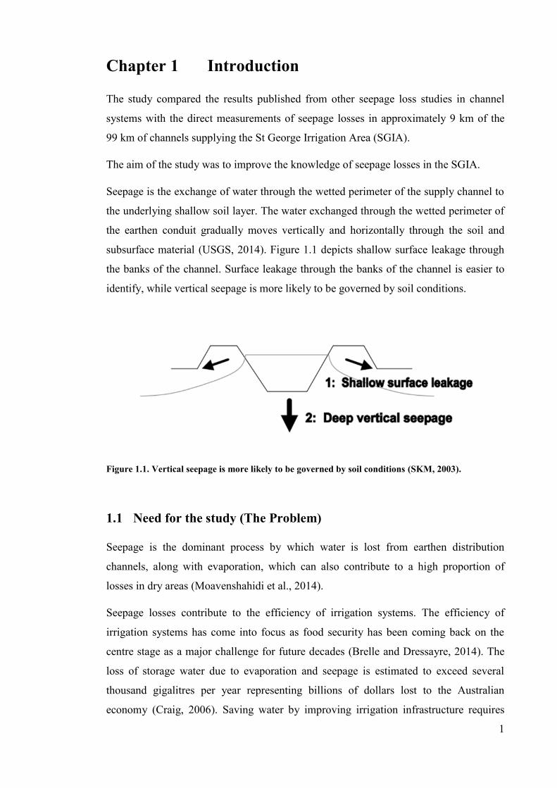
Seepage is the exchange of water through the wetted perimeter of the supply channel to
the underlying shallow soil layer. The water exchanged through the wetted perimeter of
the earthen conduit gradually moves vertically and horizontally through the soil and
subsurface material (USGS, 2014). Figure 1.1 depicts shallow surface leakage through
the banks of the channel. Surface leakage through the banks of the channel is easier to
identify, while vertical seepage is more likely to be governed by soil conditions.
Figure 1.1. Vertical seepage is more likely to be governed by soil conditions (SKM, 2003).
1.1 Need for the study (The Problem)
Seepage is the dominant process by which water is lost from earthen distribution
channels, along with evaporation, which can also contribute to a high proportion of
losses in dry areas (Moavenshahidi et al., 2014).
Seepage losses contribute to the efficiency of irrigation systems. The efficiency of
irrigation systems has come into focus as food security has been coming back on the
centre stage as a major challenge for future decades (Brelle and Dressayre, 2014). The
loss of storage water due to evaporation and seepage is estimated to exceed several
thousand gigalitres per year representing billions of dollars lost to the Australian
economy (Craig, 2006). Saving water by improving irrigation infrastructure requires
2
locating seepage ‘hotspots’ (channel sections where relatively high water loss occurs)
and quantifying water losses to facilitate investment decisions in irrigation systems
(Akbar et al., 2013). The spatial distribution of seepage rates along the channels must be
quantified to establish the economic and environmental merit of reducing conveyance
loss (Khan et al., 2009).
The seepage losses measured in this study were located in the earthen channels of a
water supply system in St George, Queensland. The earthen channels supply water from
E.J. Beardmore Dam on the Balonne River to farmers located within the SGIA. The
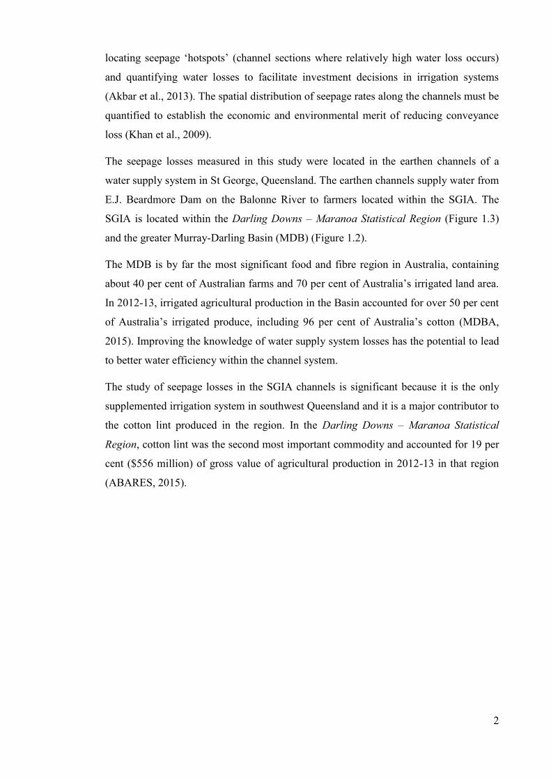
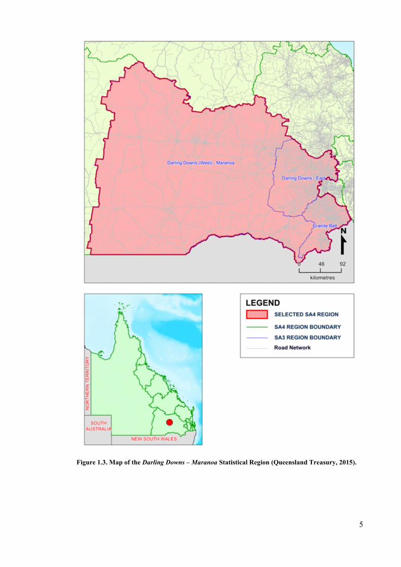
SGIA is located within the Darling Downs – Maranoa Statistical Region (Figure 1.3)
and the greater Murray-Darling Basin (MDB) (Figure 1.2).
The MDB is by far the most significant food and fibre region in Australia, containing
about 40 per cent of Australian farms and 70 per cent of Australia’s irrigated land area.
In 2012-13, irrigated agricultural production in the Basin accounted for over 50 per cent
of Australia’s irrigated produce, including 96 per cent of Australia’s cotton (MDBA,
2015). Improving the knowledge of water supply system losses has the potential to lead
to better water efficiency within the channel system.
The study of seepage losses in the SGIA channels is significant because it is the only
supplemented irrigation system in southwest Queensland and it is a major contributor to
the cotton lint produced in the region. In the Darling Downs – Maranoa Statistical
Region, cotton lint was the second most important commodity and accounted for 19 per
cent ($556 million) of gross value of agricultural production in 2012-13 in that region
(ABARES, 2015).

3
Figure 1.2. St George is located within the Murray-Darling Basin (MDBA, 2015).
Farms in the SGIA receive water via a gravity fed system of earthen channels from the
main storage, the E.J. Beardmore Dam. Transmission losses in the channels are due to
the following factors:
- Seepage (also described by infiltration to channel storage and/or floodplain
soils)
- Evaporation.
1.2 Study objective
The need for the study arises because there are no published estimates of seepage losses
in irrigation distribution systems in southwest Queensland. Therefore, the broad aim of
the study was to directly measuring seepage losses.

4
1.3 The use of seepage loss estimates
The seepage loss estimate is a portion of the loss factor used to estimate the operational
capacity to deliver water to users within the supply scheme area.
The Queensland Department of Natural Resources and Mines (DNRM) allocated shares
of the water available from the E.J. Beardmore Dam storage using historical simulations
of the SGIA (which is part of the St George Water Supply Scheme).
The simulations estimated daily stream flows, flow management, water extractions,
water demands (including operational losses) and other hydrologic events in the plan
area (Figure 2.1) between 1922 and 1995.
The average of the losses for releases from Beardmore Dam were calculated using a loss
factor of 1.15 times the supply volume – the 1.15 loss factor included all transmissions
losses (Harding, 2002) (i.e. seepage, evaporation, overflows et cetera). This means that
for every gigaltire of water released from the Beardmore Dam that 15 per cent or 150
ML of water is lost in the supply system.
The 1.15 loss factor was included in the simulation to estimate the operational capacity
to deliver water to users within the supply scheme. The exact loss factor varies
depending on the length of channel, the construction method used, vegetation,
groundwater level and soil type between the point of release and the farm gate, as well
as, climate factors, such as daily temperature, evaporation and rainfall at the time of
release (Harding, 2002).
5
Figure 1.3. Map of the Darling Downs – Maranoa Statistical Region (Queensland Treasury, 2015).

6
1.4 Research question
The history and development of the SGIA described later in Chapter 2 provides a strong
context for why water-savings are a critical area of focus for future food and fibre
security. The aim of the study is to answer the question:
- Does seepage represent a significant loss to the channel supply scheme in the
SGIA?
1.5 Objectives of the study
1. Research the background information relating to this distribution system and
seepage rates in earthen channels, measuring seepage in earthen channels and
usage of instrumentation in field measurement.
2. Design a field measurement programme to collect channel water level, and
evapotranspiration data, as appropriate.
3. Analyse field data and estimate seepage loss.
4. Research the effects that seepage loss has on efficiency in water distribution in
channel irrigation systems from other studies.
7
Chapter 2 Literature review
This chapter describes the study area and the background of the St George Water Supply
Scheme. The later sections of the chapter detail the results of other seepage loss studies
in Australia and the methods used to measure seepage loss. Finally, the chapter reviews
methods to reduce seepage losses.
2.1 Background
A reliable water source in the SGIA is a key to the future economic development and
the sustainable future of the irrigation industry in the local region. The history and
development of the SGIA provides a background understanding of how the demand for
irrigation water has increased since the St George Water Supply Scheme commenced
during the 1940s and why it is important to estimate seepage losses accurately.
2.1.1 The study area
The SGIA is part of the St George Water Supply Scheme and it is located within the
Balonne catchment of the northern MDB (Figure 2.1).
Rainfall is summer dominate in the SGIA and is influenced by the semi-arid nature of
the catchment and the average annual rainfall is 517 mm (BoM, 2015). Demands from
the distribution system are approximately 5 MLha-1
per year although these demands
are generally administered over a 7-month cotton growing cycle (GHD, 2001).
The main irrigated crop produced in the SGIA study area is cotton. There was a reduced
cotton harvest in the 2013 and 2014 seasons following the greatly reduced availability
of water due to a 10 year period of drought in Queensland (ABARES, 2014). In 2014-
15 the drought continued to affect Queensland farms subduing crop production (ABS,
2014).
Despite the decline in cotton production during the drought, cotton remains the
dominant irrigated summer crop in the upper MDB on clay soils, due to the expectations
of improved returns, relative to other summer crops (Gunawardena and McGarry,
2011).
8
Figure 2.1 shows the location of the St George Water Supply Scheme. The scheme is
located at the headwaters of the Balonne River (part of the Condamine River and
Balonne River catchments). The Condamine and Balonne catchment are the headwaters
of the Murray-Darling Basin river system that flows through Dirranbandi and Hebel
across the Queensland border to New South Wales.
2.1.1.1 Development history of the SGIA water supply
As early as 1889, the Queensland Government proposed to conserve water by building a
series of weirs on the Condamine River between Dalby and St George, but this idea was
abandoned when surveys showed that only very small storages could be constructed
along that section of the stream. Then, in 1953, the Commissioner of Irrigation and
Water Supply first presented the St George Irrigation Project (the original developed
area of the SGIA) to the Queensland Parliament. The project aimed to bring the benefits
of irrigation to the western area of Queensland. (Nimmo, 1953).
According to Nimmo, a combined concrete bridge and weir (the Jack Taylor Weir) –
was completed in 1948 for the primary purposes of providing a road crossing on the
Balonne River and a water supply for the town of St George. The surplus water stored
behind the weir was to be used as an experiment to discover what extent the benefits of
irrigation could be brought to the west.
The irrigation area developed in two stages. The first stage (the western St George Main
Channel system) was comprised of 17 farms, taking water from the quantity available
from the existing Jack Taylor Weir. The initial farms were not successful due to the
small size of the farms and low water allocations and later both of these allocations
increased when the capacity of Jack Taylor Weir increased.
In 1972, the irrigation area expanded (the eastern Buckinbah channel system) with the
opening of 32 new irrigation farms following the completion of Beardmore Dam and
associated weirs and channels. The area irrigated in the 1970s was constant at
approximate 8000 hectares. In the 1980s the irrigated area increased to approximately
9000 hectares and over the same period cotton became the dominant crop, exceeding 90
per cent of the area planted in the SGIA (QWRC, 1994).

9
Figure 2.1. The plan area for the Condamine and Balonne catchments (Queensland Government, 2015).

10
The trend in water use increased accordingly with the increase in cotton farming, and
the trend indicates that there is demand for 100 per cent of nominal allocation from
Beardmore Dam in most years. This demand has been confirmed more recently by the
Queensland Competition Authority (QCA) review of future price pathways that collated
up to 25 years of historical data for all water use and cited that SunWater (Queensland
Government Corporation, i.e. the scheme operator) assumed a water usage forecast of
95 per cent of the allocation in the river system (QCA, 2011).
Despite the increased water demand, the capacity of the channel system remained the
same, which created over-demand for water from Beardmore Dam.
The rising water demand trend occurred during a period following severe drought –
which was complicated further, following a detailed survey in 1993 that reduced the
estimated capacity of Beardmore Dam from 111 GL to 81.9 GL.
2.1.1.2 Overview of the supply system from the Beardmore Dam to the SGIA
In Australia the main mechanism for the supply of water from water supply schemes to
farms is through earthen channels (Khan et al., 2009). Beardmore Dam supplies water
through approximately 100 km of earthen channels to farms located within the SGIA
(Figure 2.2).
The E.J. Beardmore Dam is located approximately 20 km upstream from St George on
the Balonne River. The water supplied to the SGIA is gravity fed through the Balonne
River and Thuraggi Watercourse (SunWater, 2011). Since 1998, the channel operator
has controlled the water supplied within the channel system using a Supervisory Control
and Data Acquisition (SCADA) system installed at the major storages (e.g. Buckinbah
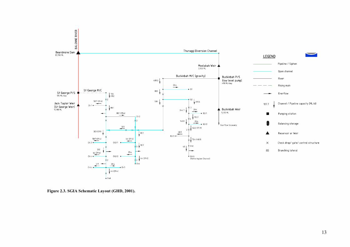
Weir) and manual gates (Figure 2.2). Figure 2.3 shows the system capacity, and the
locations of the connections between channels, pump stations, channel regulators and
channel overflows.
Water released from the Beardmore Dam flows along the Balonne River and Thuraggi
Watercourse and is supplied to the SGIA, where:
- the western portion is supplied by pumping from Jack Taylor Weir on the
Balonne River to the St George Main Channel

11
- the eastern portion is supplied by gravity via Thuraggi Watercourse released via
Moolibah Weir and Buckinbah Weir to the Buckinbah Main Channel.
The western channel system (the St George Main Channel) constructed during the
1950s was compacted earth and the eastern channel system (the Buckinbah Main
Channel) was constructed during the 1970s. The first 3 km (approximately) of the St
George Main Channel was clay lined during the 1980s. Table 2.1 shows the summary of
the construction types and lengths of the channels (GHD, 2001).
Table 2.1. Main Channel Characteristics (GHD, 2001).
Channel Total Length
[m]
Component Length [m]
Earth Unlined Clay Lined Pipe
St George Main Channel 53528 49753 2917 858
Buckinbah Main Channel 33785 33625 - 160
2.1.1.3 Estimated efficiency of the distribution system
The efficiency of water supplied to the SGIA is the ratio between water supplied to
SunWater customers and water delivered to the system (i.e. released from Beardmore
Dam).
In 1974, the maximum draft (demand plus losses) on the SGIA system was the customer
demand plus the system distribution losses and the assumed efficiency distribution for
the SGIA was 75 per cent (QWRC, 1994). Following the major expansion of the
channel system in the 1970s the estimated efficiency increased to 85 per cent under
current operating conditions (GHD, 1997). The efficiency gain was due to the increased
channel capacity and higher flow rates of the newly constructed extension area to the
east known as the Buckinbah Channel System.

12
Figure 2.2. St George Irrigation Area Locality Map (GHD, 2001).
13
Figure 2.3. SGIA Schematic Layout (GHD, 2001).

14
Despite the early development efficiency estimates cited above, there is limited
efficiency data available about the SGIA and an internal report commissioned by the
DNR estimated the annual distribution efficiency was between 76 per cent (average
operational efficiency) and 95 per cent (average theoretical efficiency) for the period
between 1993/1994 and 1997/1998 water years. GHD established these efficiency
estimates in 2001, which included distribution losses attributed to seepage and
evaporation. No efficiency data has been available since 1998 when SunWater
commenced operation of the scheme.
For the distribution system efficiency review, GHD estimated evaporation losses and
seepage rates (GHD, 2001) as shown in Table 2.2 and Table 2.3. The seepage rates
estimated by GHD were adopted based on measurements made in other Queensland
water supply systems. The pan factors reported by GHD are from Bureau of
Meteorology evaporation measurements (Table 2.2) recorded at Inglewood, Queensland
(approximately 300 km east of St George) and the adopted seepage rates (Table 2.3)
were “best guess” approximations.
Table 2.2. Average monthly evaporation at Inglewood, Queensland (mm) (GHD, 2001).
Station No. Jan Feb Mar Apr May Jun Jul Aug Sep Oct Nov Dec
043053 251 212 199 134 84 61 63 89 140 188 228 226
Pan Factors1 0.92 0.96 1.01 0.76 0.58 0.47 0.38 0.59 0.85 0.89 1.01 0.91
1. Pan factors Weeks (1991)
Table 2.3. Estimated seepage rates for the SGIA (GHD, 2001).
Channel Lining Type Seepage Rate [md-1]
Clay Lined 0.005
Unlined Earth 0.008
2.1.1.4 Water accounting in the SGIA
Water supplied through the system is regulated at a few measurement points located at
simple control structures used by the operators to change flow rates to different supply
zones in the channel system. Despite, the seemingly unsophisticated automation of the

15
water supplied to the SGIA, the operators indicated no noticeable seepage was
occurring along the channels. However, to the contrary, GHD cited irrigator
representatives suggested that particular sections of channel (through sandy soils)
showed signs of water loss through seepage (i.e. unusually green vegetation in a dry
landscape).
Individual meter outlets installed on the channel offtakes record each client’s monthly
water use. A combination of mechanical dethridge wheels (Figure 2.4) and modern
electronic ultrasonic meters measure water use. In some cases, the metering devices
measure more than one water allocation and the water user is responsible for recording
daily water use to reconcile the take of multiple water products, e.g. supplemented
supply and unsupplemented water harvesting. The advantage of the simple metering
system is that it lowers the labour/capital costs for water users and the disadvantage is
that it is naturally more open to error and time delay between the actual take of water
and record of the metered use.
Figure 2.4. A mechanical dethridge wheel is a highly reliable method of water measurement but has a lower accuracy than modern ultrasonic meters.
The delayed water use records mean that the water use record is not precise enough to
calculate accurate losses within the distribution system using flow data alone. The
measurement inaccuracies are also likely to contribute to potential errors in the
estimated operational and theoretical efficiency of the distribution system.
The overall bookkeeping (of the amount of water available in the dam for release) for
the St George Water Supply Scheme changed during 2000 as described further below.

16
Water accounting of water stored in the Beardmore Dam has been the main instrument
used to reallocate water to satisfy the increasing demand for a reliable water supply for
irrigation. Like many major irrigation water storages in Australia, water supplied to the
SGIA was historically on an announced allocation basis. In an announced allocation
system the available water for each season is determined by the water operator based on
the amount of water available for use at the commencement of the water year or
irrigation season given prevailing storage levels (Hughes and Goesch, 2008).
In 2000, the capacity share (also known as continuous sharing) water accounting system
replaced the announced allocation water accounting system used to manage the water in
storage in the St George Water Supply Scheme.
The capacity share water accounting system is a decentralised approach, cited by
Hughes and Goesch (2008), as first being proposed by Dudley in 1988, where irrigators
can make their own storage decisions. The capacity share system allocated a share of
the total storage capacity (as well as a share of inflows into, and losses from, the
storage) to each water user, rather than a share of total releases for the season.
In the capacity share system, each water user manages their shares of total storage
capacity independently, determining how much water to use and how much to store for
the future (Hughes and Goesch, 2008).
This method of water accounting helps irrigators decide the area of crop to plant and
their investment in crop inputs based on the share of the total available storage capacity
and a predicted crop yield forecast on an annual basis. However, equally, the flexibility
in this water accounting system and water demand provides a challenge for the operator
who must now attempt to distribute the water flow based on less predictable flows
required within different zones of the distribution system, which influences the
available daily channel capacity.
2.1.2 Key issues facing the St George district
The economy of the St George district relies heavily on irrigated agricultural
production. Almost 40 per cent of the population of the surrounding Balonne shire is
employed in the agricultural industry (Queensland Government Statician's Office,
2015). The semi-arid climate means that annual production is strongly dependant on
rainfall and a reliable water supply scheme.

17
The key issue facing the St George district is meeting the future demand for food and
fibre with potentially less available water and the flow on effects for the local economy.
Therefore, improving water loss estimates (such as seepage losses) should be studied to
better understand the overall contribution to water losses within the SGIA distribution
system.
This study seeks to improve the knowledge about seepage losses in the SGIA. There are
two main areas that may greatly benefit from a better understanding of the seepage
losses. The three main areas are:
1. the operational arrangements of the channel
2. farm watering decisions (improving the efficiency of on- and off- farm irrigation
infrastructure).
2.1.2.1 Operational arrangements
The operational arrangements are impacted by the capacity of the channel system to
deliver water to SunWater customers. The capacity of the channel system was based
originally upon the principle of supplying 5 ML per hectare of irrigable land. Based on
these calculations peak flow rates in the channel system were determined for individual
parcels of land. These peak flow rates also made allowances for the hydraulic
limitations of the individual channel sections (SunWater, 2015). The primary limitation
of the SGIA channel system is that the peak hydraulic demand of the distribution
system exceeds the design capacity of the channel delivery system. The peak operation
of the channel is restricted further by the principal transmission losses, discussed
elsewhere in the report, but may also be impacted by irrigation demand (seasonal)
within sections of the channel system and channel maintenance.
To overcome the system capacity limitation, all of SunWater’s customers must adhere
to peak flow rates to share channel capacity during periods when demand for water
exceeds the system’s capacity to delivery.
Improving the understanding of seepage loss in the channel system has the potential to
support future infrastructure investments, such as, future channel maintenance aimed at
improving peak/delivery flow rates.

18
2.1.2.2 Farm watering
Water users use the available water in storage at the beginning of the growing season to
estimate the area of crop to plant and DNRM rely on the IQQM computer simulation
program to understand the long-term security of each water user’s allocation. The
IQQM calculates the historical availability of water using streamflow recorded at
gauging stations, climate and land data based on allocated water user demands. The
long-term availability of the water can be used to temporarily or permanently move the
point of take of the water to suite water user demand (trading).
When a water user decides to trade water the availability of water is recalculated at the
new location or at the same location under the reduced volume using the IQQM. There
are two outcomes from the simulation:
- the DNRM can use the simulation as evidence that the average volume of water
available remains the same in the proposed location following the trade
- water users use the estimate of long-term diversions to give an indication of the
amount of water that will be available from the regulated system, so that they
can plan their crop areas. The growers can use the estimate to forecast their risk
profile and investment based on the availability of water at the beginning of the
growing season.
Improving the understanding of seepage loss in the distribution system has the potential
to improve the knowledge of water availability used by growers to plan crop plantings.
2.2 Water distribution losses in channel distribution systems
The main water supply losses in earthen channels are due to the following factors:
- seepage losses
- evaporation losses.
Other water losses may include overflows and theft.
According to Sonnichsen (1993) the seepage rate is controlled mainly by the effective
hydraulic continuity of the underlying base material, conveyance material, and the
hydraulic gradient.

19
The size of the soil particles and the pore space between the soil particles determine the
pathways for water to transmit from the channel bed and banks through the underlying
base material. The hydraulic gradient is the difference between the pressure exerted on
the soil surface by the column of water in the channel and the saturation of the
underlying base material. The saturation pressure of the underlying base materials can
be influenced by the conductivity of the nearby groundwater storage. For any given
degree of soil saturation, the hydraulic conductivity increases going from clay to sand
particles. With small pores there is a higher resistance to flow and with large pores there
is less resistance to flow.
Smith (1982) cited the distribution of irrigation water through a system of earthen
channels must result in seepage from earthen channels, and that seepage loss is one of
the largest remaining, but least definable, sources of water loss in the irrigation systems
(of Northern Victoria).
Seepage loss from any supply system can vary, but Sonnichsen (1993) cited
Christopher’s (1981) estimate of 25 per cent of any diversion/release to be an average
amount lost to seepage. Another factor on estimates cited by Moavenshahidi et al.
(2014), during a 3 year study, affecting the accuracy of the estimated seepage rates was
seasonal variation. For example, during a 3 year study, the estimated seepage rate was
almost 60 per cent higher in August than the rate estimated for September.
Hence, seepage rates vary widely throughout the year and a variation in rates is not
unusual especially where silt or sealing takes place over a period of time (United States
Department of the Interior, 1968) and as groundwater levels change during the season.
All of the seepage loss studies reviewed concluded that seepage losses reduced the
efficiency of water distribution; however, the cost benefit of reducing seepage losses
(discussed in section 2.4) can be prohibitive.
2.2.1 Australian seepage loss studies
The review of available Australian seepage studies showed that seepage varied between
0.002 md-1
and 0.088 md-1
. Table 2.4 shows the summary of the review. The seepage
loss studies focussed mainly on supply systems located in Victoria and Western
Australia. The summary shows the location, the lower and upper limits of the seepage
rates and the measurement technique used during the study. There is a large range of
20
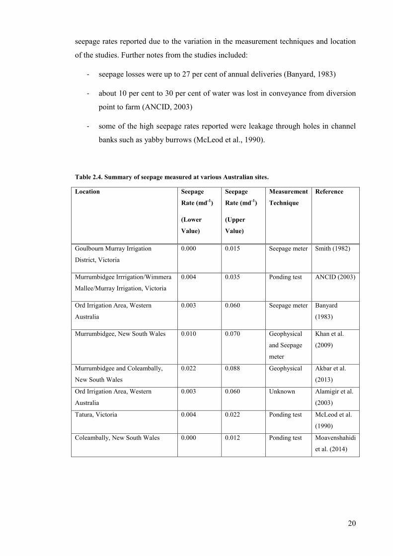
seepage rates reported due to the variation in the measurement techniques and location
of the studies. Further notes from the studies included:
- seepage losses were up to 27 per cent of annual deliveries (Banyard, 1983)
- about 10 per cent to 30 per cent of water was lost in conveyance from diversion
point to farm (ANCID, 2003)
- some of the high seepage rates reported were leakage through holes in channel
banks such as yabby burrows (McLeod et al., 1990).
Table 2.4. Summary of seepage measured at various Australian sites.
Location Seepage
Rate (md-1)
(Lower
Value)
Seepage
Rate (md-1)
(Upper
Value)
Measurement
Technique
Reference
Goulbourn Murray Irrigation
District, Victoria
0.000 0.015 Seepage meter Smith (1982)
Murrumbidgee Irrrigation/Wimmera
Mallee/Murray Irrigation, Victoria
0.004 0.035 Ponding test ANCID (2003)
Ord Irrigation Area, Western
Australia
0.003 0.060 Seepage meter Banyard
(1983)
Murrumbidgee, New South Wales 0.010 0.070 Geophysical
and Seepage
meter
Khan et al.
(2009)
Murrumbidgee and Coleambally,
New South Wales
0.022 0.088 Geophysical Akbar et al.
(2013)
Ord Irrigation Area, Western
Australia
0.003 0.060 Unknown Alamigir et al.
(2003)
Tatura, Victoria 0.004 0.022 Ponding test McLeod et al.
(1990)
Coleambally, New South Wales 0.000 0.012 Ponding test Moavenshahidi
et al. (2014)
21
2.2.2 Other seepage loss studies outside of Australia
The bulk of seepage studies outside of Australia found during the review were in the
United States of America (USA) and there was a significant difference to the rate of
seepage measured in Australian conditions. The rates appeared to be lower than for
Australian conditions. Although there were more recent studies, the results of the
seepage loss studies have not varied greatly since first published by the United States
Bureau of Reclamation in 1968.
According to the United States Bureau of Reclamation (1968), a well compacted or
“tight” channel might have a seepage rate of 0.003 md-1
or a seriously leaking unlined
channel might have a seepage rate of 0.017 md-1
or higher. A summary of the results of
the study are shown later in the Chapter in Figure 2.6.
A variety of measurement techniques were used to complete the studies on water supply
systems that were developed before the Australian systems. The summary in Figure 2.6
also shows additional data for seepage rates of linings other than compacted earth,
whereas, the Australian studies only show the seepage rates for compacted earth
channels.
2.3 Methods to measure seepage losses
According to Khan et al. (2009), commonly used methods for identifying seepage are:
- Local quantitative seepage estimates using the Idaho seepage meter (Shinn et al.,
2002)
- Ponding tests to determine bulk seepage from and isolated channel reach
- Inflow-outflow tests to determine bulk seepage from channel reaches
- Geophysical methods.
2.3.1 The Idaho Seepage Meter
Seepage meters are a point measurement used when the channel is operating or when it
is not running. This usually involves the application of water to the surface or hole
within the channel and measurement of the rate of water loss. The infiltration rate has a
22
direct relationship to the seepage at that point and can be useful for identifying seepage
hotspots and relative seepage potential.
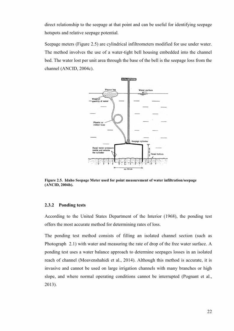
Seepage meters (Figure 2.5) are cylindrical infiltrometers modified for use under water.
The method involves the use of a water-tight bell housing embedded into the channel
bed. The water lost per unit area through the base of the bell is the seepage loss from the
channel (ANCID, 2004c).
Figure 2.5. Idaho Seepage Meter used for point measurement of water infiltration/seepage (ANCID, 2004b).
2.3.2 Ponding tests
According to the United States Department of the Interior (1968), the ponding test
offers the most accurate method for determining rates of loss.
The ponding test method consists of filling an isolated channel section (such as
Photograph 2.1) with water and measuring the rate of drop of the free water surface. A
ponding test uses a water balance approach to determine seepages losses in an isolated
reach of channel (Moavenshahidi et al., 2014). Although this method is accurate, it is
invasive and cannot be used on large irrigation channels with many branches or high
slope, and where normal operating conditions cannot be interrupted (Pognant et al.,
2013).

23
In this test, existing check structures can be used to pond water in an isolated channel
section – where, canvas or plastic is usually placed over the upstream side to cover open
joints and to prevent leakage around the isolating structure.
The test equipment used is a water stage recorder in a stilling well to measure the rate of
drop in the water surface and in some cases an evaporation pan. If the pond is long or
subject to wind conditions, the recorders are paired for use at upstream and downstream
ends of the pond. By having gauges at each end, average water surface elevation can be
determined. Each recorder should be referenced to water surface elevation so that
depths of water in the pond can be compared with design or operating depth. A check
on the recorder may be made when the pond water surface is absolutely still so that the
water surface elevation can be calibrated with the recorder.
Evaporation pans and rain gauges are not usually necessary; however, if evaporation is
significant in a pond with a low loss rate, an evaporation pan should be installed or may
be obtained from a nearby weather station representative of the test site.
A survey to establish the as-built shape and length of the pond is usually required. From
the survey of the pond, the water surface width according to elevation and wetted
perimeter according to elevation are established and volumes of water losses are
calculated.
Photograph 2.1. Existing check structures like the one shown here can be used to pond water in isolated channel sections.

24
2.3.3 Inflow-outflow tests
The inflow-outflow method consists of performing both upstream and downstream
discharge measurements, as well as time series of depth measurements and compares
the values obtained in those channel sections. The main advantage of this approach is
losses are measured under the normal operating conditions of the channel. The major
disadvantage of this method is the need for a large number of very accurate flow
measurements over time and the impossibility to identify localised losses (Pognant et
al., 2013).
When considering the accuracy of the measurements, Fairweather et al. (2009)
recommended that after identifying the boundaries of the channel sections and delivery
system and the time-frame for the test, the confidence that can be placed in them should
be reported. In some cases, the error in the measurement of the inflow-outflow test may
be many times greater than the magnitude of the seepage loss. This means that there is a
larger opportunity for error in the inflow-outflow technique unless the operator is very
confident that the measurements are very accurate for the duration of the test.
2.3.4 Geophysical methods
Seepage loss depends on soil properties. One method that used for decades for mapping
soil properties is Electromagnetic Induction (EM). EM is fast and user friendly, easy for
field applications and not excessively expensive (Pognant et al., 2013). EM devices
work on the theory that within an electromagnetic field any conductive object carries a
current. The instrument measures the soil apparent Electrical Conductivity. Each
instrument has two coils (a transmitter and a receiver) that are placed at either a fixed or
variable distance apart. EM does not provide quantitative seepage rates and the data
collected by the devices must be interpreted based on the apparent Electrical
Conductivity of the soil, hence, the same Electrical Conductivity may have different
seepage rates.
The instrument induces an electrical current into the soil, with depth penetration
determined by the separation of the coils and the frequency of the current. Electrical
Conductivity is affected by the soil’s salt content and type, clay content and type,
mineralogy, depth to bedrock, soil water content, organic matter and exposure. The
depths reached by the signal will be determined by the uniformity of the soil. If the soil

25
is very conductive near the surface then the signal will be dissipated and will not go
deeper (Pognant et al., 2013). Ideally, replicate EM electrical conductivity
measurements are performed while the channel is operating during a permanent flow in
steady operating conditions.
2.3.5 Summary of testing methods and method selected for the study
Based on the availability of the suitable short sections of isolated channel in the SGIA,
equipment and time resources available the ponding test method was selected to
measure seepage losses.
Due to the limited time resources and inaccurate inflow/outflow measurements available
during the study period the seepage meter method, the inflow/outflow test and the EM
method presented major impediments.
The major disadvantage with the seepage meter method was the labour-intensive nature
and inability to quantify distributed seepage losses along the length of the canal.
Similarly, the inflow-outflow and geophysical methods required access to a large
number of very accurate measurements over time.
The ponding method was the preferred method cited by the Channel Seepage
Management Tool and Best Practice Guidelines for identifying and measuring seepage
in channel network published by the Australian Government (ANCID, 2003). More
recently, the Commonwealth Scientific and Industrial Research Organisation (CSIRO,
2008) published the Technical Manual for Assessing Hotspots in Channel and Piped
Irrigation Systems that recommended that the best application for defining water loss
hotspots was a seepage meter, whereas, the pondage test was considered the most
accurate method for assessing channel seepage.
Many sources (Moavenshahidi et al., 2014, Sonnichsen, 1993, United States
Department of the Interior, 1968) cited ponding tests are acknowledged as the most
accurate direct method for seepage measurement in irrigation channels for relatively
short sections of channel because of the substantial improvement in the accuracy of the
seepage estimate. However, the method involved a considerable cost and disruption to
the operation of the channel, unless used only at the end of the irrigation season.

26
2.4 Methods to reduce seepage loss
The two most common solutions reported for reducing seepage were lining channels or
replacing them with pipes Burt (2008), however, these solutions are expensive. Lining
channels was not the only method to reduce seepage found during the literature review.
Typical linings included compacted earth, concrete, plastic membrane, and plastic pipe
(Sonnichsen, 1993). Other methods to reduce seepage included, changing the design
geometry of the channels to reduce the wetted perimeter, compatible soil compaction
techniques during construction and lining of channels with inactive materials. Burt
(2008) reported in-situ compaction for sandy loam soils in California with vibratory
roller reduced seepage by 89 per cent when both sides and bottom were compacted; and
cited the ANCID (2001) Open Channel Seepage and Control, Vol. 2.1 as the best source
for information on earth lining of channels.
The different lining methods reduced seepage but losses even under ideal operating
conditions were not eliminated unless the earthen channel was replaced by a closed pipe
system. Figure 2.6 shows the summary of the review of various seepage rates and lining
treatments.
- Compacted earth lining was reported to reduce seepage to below 0.002 md-1
with
an expected design life of 20 years (Kraatz, 1977, Sonnichsen, 1993)
- Unreinforced concrete linings of 0.076 m thickness were reported to reduce
seepage to 0.009 md-1
when new; with a life span of 50 years.
Sonnichsen cited findings by Worstell (1976) where channel seepage rates for broad
soil textural groups were evaluated by analysing results of 765 tests made in the western
United States where seepage rates varied between 0.006 md-1
and 0.060 md-1
.

27
Figure 2.6. Seepage rates for typical linings (Sonnichsen, 1993).
Figure 2.6 illustrates the relationship between hydraulic conductivity and the effect of
difference channel linings, seepage and soil properties described earlier in Chapter 2.
The measurements in Figure 2.6 are reported in US Customary Units of feet per day, 0.1
and 1 ftd-1
correspond to 0.00305 md-1
and 0.0305 md-1
. For example, large soil particle
sizes, such as gravels, have a greater pore space in the soil matrix and conduct water
better (1.22 md-1
) than smaller soil particles such as a clay loam (0.107 md-1
). The
seepage rates for typical linings demonstrates that as the pore space in the lining
becomes smaller that there will be less seepage.
In 1973, a three year study on factors contributing to natural sealing of irrigation
channels was published by the Water Resources Research Institute, University of Idaho
(Brockway, 1973). Brockway evaluated the effect of sedimentation, microbiological
activity and soil-water chemical reactions on the hydraulic conductivity of soils,
particularly, in the Portneuf silt-loam soil of southern Idaho.
According to Brockway (1973) earthen channels developed a natural lining with age.
The investigation of this ageing process identified two components, the depositions of
mineral colloids in a natural lining and biological activity within the lining. When well
developed, this natural lining effectively controlled the rate of seepage, that is, the
seepage rate was independent of the subsoil hydraulic conductivity. Brockway
concluded the long-term reduction in seepage rates of channels constructed in silt-loam

28
soils was due to the formation of an impeding layer on the channel bottom due primarily
to sedimentation.
Later in 1982, the evidence measured in Australia by Smith also suggested that the
natural ageing of earthen channels resulted in a reduction in seepage to a value
comparable with that achieved by constructed linings (e.g. plastic, clay, concrete).
Smith suggested artificial linings that complement (and perhaps even accelerated) the
natural sealing process achieved the most economical result.
All of the studies reviewed recommended that prior to any channel remediation works
the benefits of the capital cost of construction must be considered. For example, a
remediation technique may have a cheap capital cost, but it may need replacing every
year, and an alternative option may be expensive but have a 50-year life.
The calculation of remediation cost depends on the rate of seepage identified, the water
savings estimated by replacing the channel lining/construction and the cost to mobilise
plant, equipment and materials to site. While there are some costs published in the
literature, they are not easily applied to all channel remediation works in different
locations, however, ANCID (2004a) published a manual to evaluate channel
remediation works which takes these and other factors into consideration.
2.5 Conclusion
The SGIA is a key cotton production area located in southwest Queensland. The
economy of the St George district (in the Balonne shire) relies heavily on agricultural
production. Rainfall in the study area is summer dominant and average annual rainfall is
517 mm. Water for irrigation to supplement rainfall is supplied by a channel system
(part of the St George Water Supply Scheme) to irrigate approximately 9000 hectares of
cotton and horticulture in the SGIA. The key issue facing the SGIA is meeting the
future demand for food and fibre with potentially less water available.
The channel system delivers water stored in the Beardmore Dam to farms in the SGIA
using approximately 99 km of compacted earthen channels. The estimated efficiency of
the system is between 76 per cent and 95 per cent of water released from the dam. The
performance of the system is reduced by water losses. The main water losses in the
channel system are due to evaporation and seepage losses; other losses may include
overflows and theft. A loss factor of 1.15 is used to estimate losses.
29
There are currently no published estimates of seepage losses in irrigation systems in
southwest Queensland. Therefore, improving water loss estimates, such as seepage
losses, should be studied to better understand the overall contribution of water losses
within the SGIA distribution system. The lack of the known seepage losses limits the
ability to estimate improved delivery strategies. This chapter reviewed other seepage
losses studied in Australia and overseas.
The seepage rate is controlled mainly by the effective hydraulic conductivity of the
underlying base material. Seepage loss rates studied in Australian channel systems vary
between 0.002 md-1
and 0.088 md-1
.
There are four main methods to measure seepages losses. The ponding test was used for
recommended as the most accurate method.
Natural sealing of earthen irrigation channels may occur due to sedimentation,
microbiological activity and soil-water chemical reaction on the hydraulic conductivity
of soils with age. Once the seepage rate is determined, the two main methods to reduce
seepages losses are lining channels or replacing them with pipes. All of the other
seepage loss studies reviewed concluded that seepage losses reduce the efficiency of
water distribution; however, the cost benefit of reducing seepage losses (Section 2.4)
can be prohibitive.
Chapter 3 follows to discuss the available techniques in relation to the experimental
techniques and equipment used to measure seepage losses in this study.
30
Chapter 3 Experimental techniques and equipment
The aim of the study was to directly measure seepage losses in the channel system that
supplied the SGIA. This chapter describes the design of the measurement sites and how
water depths were measured during the ponding tests.
The objective of the experimental design was to minimise the equipment housing space
requirements and to maintain safe access to the instruments while producing the most
accurate results possible.
3.1 Introduction
This section describes the characteristics of the soil and vegetation located at each site
and the site selection process.
The site selection began in November 2014. The initial criteria used to select the sites
were remnant vegetation and high channel supply capacity. The secondary selection
reviewed the field observations during the initial inspection and compared the detailed
QWRC soil mapping compiled during the original investigation of the SGIA in the
1950s. The final criteria identified a length of channel between two check structures to
isolate a ponded length during shutdown periods.
The measurement sites were installed during two field trips between December 2014
and January 2015.
The sites were located within 20 km of the St George Airport weather station 043109,
(Bureau of Meteorology) site which published daily measured rainfall and
evapotranspiration derived from automatic weather station records.
3.2 Measurement sites
The three sites were:
- Site 1: St George Main Channel
- Site 2: Buckinbah B2 Channel
- Site 3: Buckinbah B2/2 Channel.
31
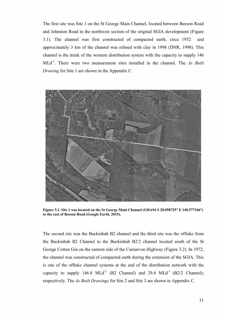
The first site was Site 1 on the St George Main Channel, located between Beeson Road
and Johnston Road in the northwest section of the original SGIA development (Figure
3.1). The channel was first constructed of compacted earth, circa 1952 and
approximately 3 km of the channel was relined with clay in 1998 (DNR, 1998). This
channel is the trunk of the western distribution system with the capacity to supply 146
MLd-1
. There were two measurement sites installed in the channel. The As Built
Drawing for Site 1 are shown in the Appendix C.
Figure 3.1. Site 1 was located on the St George Main Channel (GDA94 S 28.058725° E 148.577346°) to the east of Beeson Road (Google Earth, 2015).
The second site was the Buckinbah B2 channel and the third site was the offtake from
the Buckinbah B2 Channel to the Buckinbah B2/2 channel located south of the St
George Cotton Gin on the eastern side of the Carnarvon Highway (Figure 3.2). In 1972,
the channel was constructed of compacted earth during the extension of the SGIA. This
is one of the offtake channel systems at the end of the distribution network with the
capacity to supply 146.8 MLd-1
(B2 Channel) and 29.4 MLd-1
(B2/2 Channel);
respectively. The As Built Drawings for Site 2 and Site 3 are shown in Appendix C.

32
Figure 3.2. Site 2 and Site 3 were located east of the intersection between McDonald Road and Carnarvon Highway on the Buckinbah B2 Channel (GDA94 S 28.168073° E 148.726985°) and Buckinbah B2/2 Channel offtakes (GDA94 S 28.168295° E 148.727715°); respectively (Google Earth, 2015).
All of the measurement sites were located in trapezoidal channel sections as shown in
the Type Cross Section Figure 3.3. The hydraulic properties of the channels are in Table
3.1.
Figure 3.3. The measurement sites were located in trapezoidal channels (Irrigation and Water Supply Commission Queensland, 1972a).

33
Table 3.1. Hydraulic properties for each site (DNR, 1998, Irrigation and Water Supply Commission Queensland, 1972a, Irrigation and Water Supply Commission Queensland, 1972b).
Channel Chainage
[m]
Capacity
[cumecs]
Bed Width (B)
[m]
Water Depth (d)
[m]
Total Depth of Channel
(D) - [m]
Site 1 547 - 3550 1.60 3.0 1.2 1.7
Site 2 8868 –
10753
1.70 5.5 0.8 1.3
Site 3 0 – 1393 0.34 5.5 1.1 1.5
3.2.1 Site 1: St George Main Channel
Site 1, the St George Main Channel was a clay lined earth channel. The design drawing
indicated the thickness of the clay lining was 0.4 m. The water in the St George Main
Channel is accessed by horticultural farmers (i.e. grapes, onions) a Lucerne grower and
domestic water users.
The soil properties of the channel material were determined by reviewing remnant
vegetation and the available soil mapping. The predominant Australian Soil
Classification Soil Orders are Sodosols and Tenosols. The CSIRO cited the length of
the St George Main Channel was constructed in sandy or loamy duplex soils; deep
cracking clays (Woodward, 1974).
Tenosols generally have a low fertility and low water-holding capacity. Tenosols are
poorly developed which typically means that they are very sandy without obvious
horizons but widespread throughout Australia and can be shallow and stony. Generally,
Tenosols have a very low agricultural potential and low water-holding capacity (Gray
and Murphy, 2002).
Sodosols are texture-contrast soils with impermeable subsoils due to the concentration
of sodium (Figure 3.4). These soils occupy a large area of inland Queensland. Generally
Sodosols have a low-nutrient status and are very vulnerable to erosion and dryland
salinity when vegetation is removed (Queensland Government, 2013). The parent
material for the Sodosol is fine sandy and clayey alluvium with a hard setting surface.
The typical land use for Sodosols is grazing of native pastures with some cropping in
better rainfall areas. The A horizon texture-contrast soil is strongly sodic and not
strongly acid in the upper 0.2 m of the red clayey B horizon (CSIRO, 2013a). Generally,
Sodosols have very low agricultural potential with poor structure and low permeability
(Gray and Murphy, 2002).

34
Figure 3.4. The typical remnant vegetation cover on a sodosol shown here in profile is the tall poplar box woodland (CSIRO, 2013a).
The remnant vegetation cover nearby Site 1 was sparse open forest of Poplar box
(Figure 3.4) (Eucalptus populnea) woodland on Cainozoic alluvial plains, this
ecosystem was extensively cleared or modified by grazing (DEHP, 2015, DSITIA,
2015). Poplar box subsoils are usually a heavy impermeable clay, with surface soils
ranging from light loamy sand in the west of Queensland increasing in texture to clays
in the east of the state (Anderson, 2003).
During the initial inspection of Site 1 (Figure 3.1) the field observations made were:
- Starting at the intersection of the channel at Beeson Road the first check
structure on the western side of the road was located at [GDA94 S 28.058792°,
E 148.577186°] – the water in the channel was syphoned underneath the road.
The bordering land was grazed for approximately the first kilometre. Next, the
water in the channel was syphoned under the Commissioners Point Road. After
the Commissioners Point Road syphon, the land adjacent to the channel was drip
irrigation of cotton and onions (the drip irrigation was most likely due to the
sandy soil). The ponded section (Photograph 3.1) finished at the Johnston Road
check structure located at [GDA94 S 28.062296°, E 148.606482°]. No
observations were made of noticeably wet or sodden ground adjacent to the
channel. The soil type on the access track was noticeably smaller clay particles
and with a small amount of water ribboned well indicating a good clay content
in the sample.
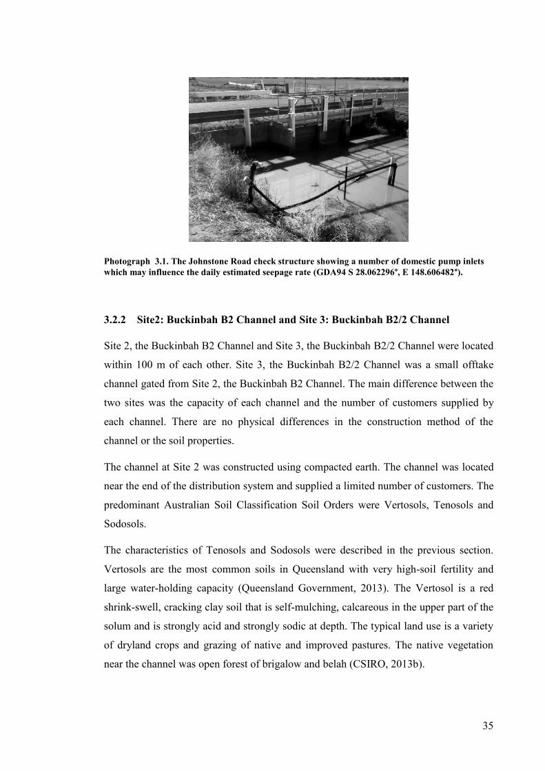
35
Photograph 3.1. The Johnstone Road check structure showing a number of domestic pump inlets which may influence the daily estimated seepage rate (GDA94 S 28.062296°, E 148.606482°).
3.2.2 Site2: Buckinbah B2 Channel and Site 3: Buckinbah B2/2 Channel
Site 2, the Buckinbah B2 Channel and Site 3, the Buckinbah B2/2 Channel were located
within 100 m of each other. Site 3, the Buckinbah B2/2 Channel was a small offtake
channel gated from Site 2, the Buckinbah B2 Channel. The main difference between the
two sites was the capacity of each channel and the number of customers supplied by
each channel. There are no physical differences in the construction method of the
channel or the soil properties.
The channel at Site 2 was constructed using compacted earth. The channel was located
near the end of the distribution system and supplied a limited number of customers. The
predominant Australian Soil Classification Soil Orders were Vertosols, Tenosols and
Sodosols.
The characteristics of Tenosols and Sodosols were described in the previous section.
Vertosols are the most common soils in Queensland with very high-soil fertility and
large water-holding capacity (Queensland Government, 2013). The Vertosol is a red
shrink-swell, cracking clay soil that is self-mulching, calcareous in the upper part of the
solum and is strongly acid and strongly sodic at depth. The typical land use is a variety
of dryland crops and grazing of native and improved pastures. The native vegetation
near the channel was open forest of brigalow and belah (CSIRO, 2013b).

36
Detailed soil mapping was available for the Buckinbah expansion area where the Site 2
and Site 3 channels were located. The channel crosses clay, then traverses
approximately 900 m of deep sands vegetated by carbeen (Moreton Bay ash) trees, 400
m of weakly solodized solonetz before returning to a further 1000 m of deep sands.
Figure 3.5. The gilgaied landscape shown on the right of the Vertosol profile originally supported an open forest of brigalow (CSIRO, 2013b).
The remnant vegetation cover was brigalow and belah and the ground layer of the
remnants of this regional ecosystem was often extensively modified by grazing (DEHP,
2015, DSITIA, 2015). The deep sand soils are noticeably vegetated by carbeen trees
which prefer lower slopes, with alluvial, often sandy soils (Anderson, 2003).
During the initial inspection of Site 2 and Site 3 (Figure 3.2) the field observations
made were:
- Starting near the intersection of Bundoran Road, the first check structure was a
set of 4 x 60 MLd-1
gates (Photograph 3.2) located at [GDA94 S 28.152885°, E
148.772466°], the adjacent land was grazed and noticeably populated by carbeen
trees on sandy soils. The terminating check structure) was located at the
intersection of McDonald Road with an unnamed road [GDA94 S 28.180524°, E
148.692948°]. The soil type on the access track was noticeably median course
sandy particles and with a small field sample did not ribbon well indicating a
lower clay content.
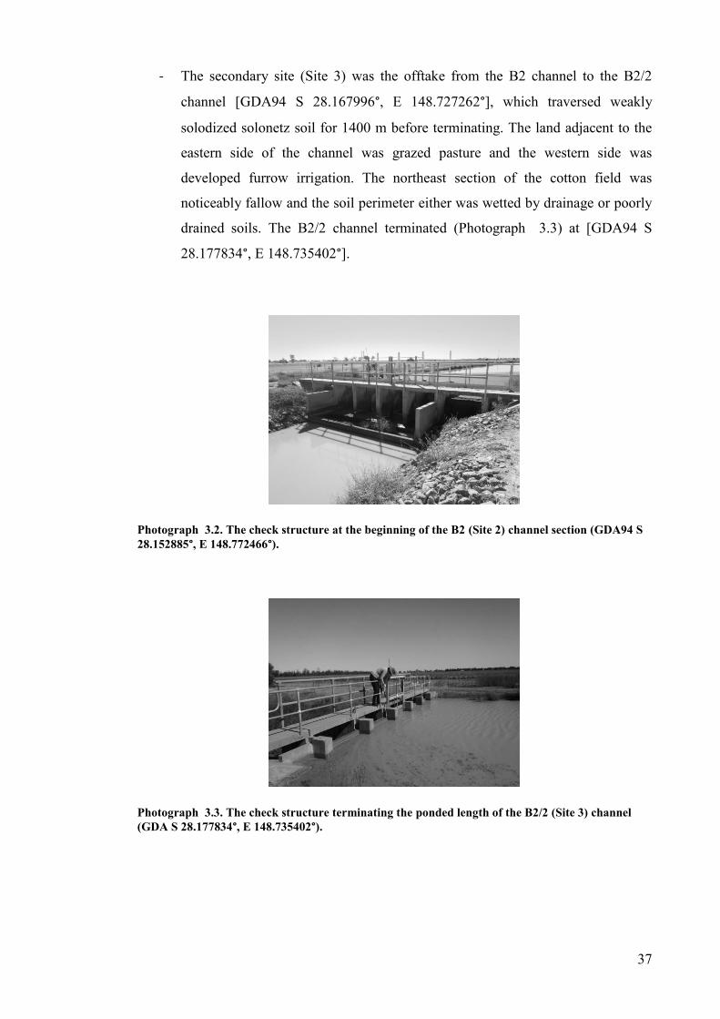
37
- The secondary site (Site 3) was the offtake from the B2 channel to the B2/2
channel [GDA94 S 28.167996°, E 148.727262°], which traversed weakly
solodized solonetz soil for 1400 m before terminating. The land adjacent to the
eastern side of the channel was grazed pasture and the western side was
developed furrow irrigation. The northeast section of the cotton field was
noticeably fallow and the soil perimeter either was wetted by drainage or poorly
drained soils. The B2/2 channel terminated (Photograph 3.3) at [GDA94 S
28.177834°, E 148.735402°].
Photograph 3.2. The check structure at the beginning of the B2 (Site 2) channel section (GDA94 S 28.152885°, E 148.772466°).
Photograph 3.3. The check structure terminating the ponded length of the B2/2 (Site 3) channel (GDA S 28.177834°, E 148.735402°).
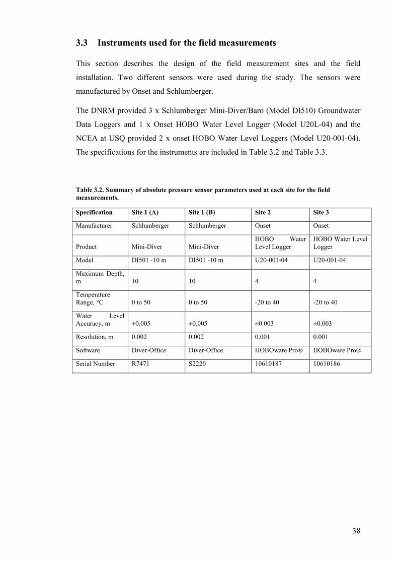
38
3.3 Instruments used for the field measurements
This section describes the design of the field measurement sites and the field
installation. Two different sensors were used during the study. The sensors were
manufactured by Onset and Schlumberger.
The DNRM provided 3 x Schlumberger Mini-Diver/Baro (Model DI510) Groundwater
Data Loggers and 1 x Onset HOBO Water Level Logger (Model U20L-04) and the
NCEA at USQ provided 2 x onset HOBO Water Level Loggers (Model U20-001-04).
The specifications for the instruments are included in Table 3.2 and Table 3.3.
Table 3.2. Summary of absolute pressure sensor parameters used at each site for the field measurements.
Specification Site 1 (A) Site 1 (B) Site 2 Site 3
Manufacturer Schlumberger Schlumberger Onset Onset
Product Mini-Diver Mini-Diver
HOBO Water
Level Logger
HOBO Water Level
Logger
Model DI501 -10 m DI501 -10 m U20-001-04 U20-001-04
Maximum Depth,
m 10 10 4 4
Temperature
Range, °C 0 to 50 0 to 50 -20 to 40 -20 to 40
Water Level
Accuracy, m ±0.005 ±0.005 ±0.003 ±0.003
Resolution, m 0.002 0.002 0.001 0.001
Software Diver-Office Diver-Office HOBOware Pro® HOBOware Pro®
Serial Number R7471 S2220 10610187 10610186

39
Table 3.3. Summary of the absolute pressure sensor parameters used for the barometric pressure measurements.
Specification Site 1 Site 3
Manufacturer Schlumberger Onset
Product Baro-Diver HOBO Water Level Logger
Model DI 500 U20L-04
Maximum Depth, m 1.5 4
Temperature Range, °C -10 to 50 -20 to 50
Water Level Accuracy, m ±0.005 ±0.1% FS
Resolution, m 0.001 0.001
Software Diver-Office HOBOware Pro®
Serial Number S4714 10662733
The site installation materials are shown in Photograph 3.4.
Photograph 3.4. The field installation of the pressure transducers was completed using hand tools and readily available materials.
Photograph 3.5 and Photograph 3.6 show the final Site 1 installations located on the St
George Main Channel. A swivel clamp bolted to the steel conduit anchored the conduit
(placed over a star picket) to the embankment. The 40 mm steel tube was sloped down
the embankment so the pressure transducer was located near the deepest part of the
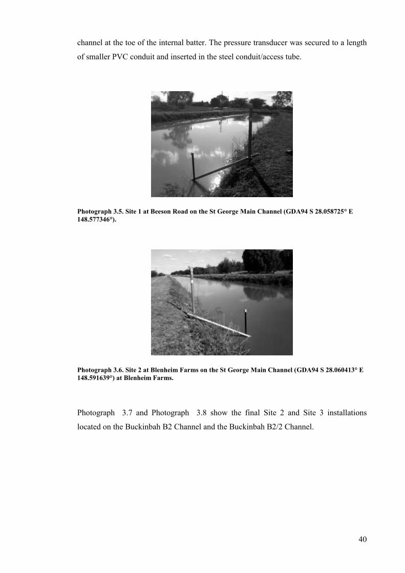
40
channel at the toe of the internal batter. The pressure transducer was secured to a length
of smaller PVC conduit and inserted in the steel conduit/access tube.
Photograph 3.5. Site 1 at Beeson Road on the St George Main Channel (GDA94 S 28.058725° E 148.577346°).
Photograph 3.6. Site 2 at Blenheim Farms on the St George Main Channel (GDA94 S 28.060413° E 148.591639°) at Blenheim Farms.
Photograph 3.7 and Photograph 3.8 show the final Site 2 and Site 3 installations
located on the Buckinbah B2 Channel and the Buckinbah B2/2 Channel.
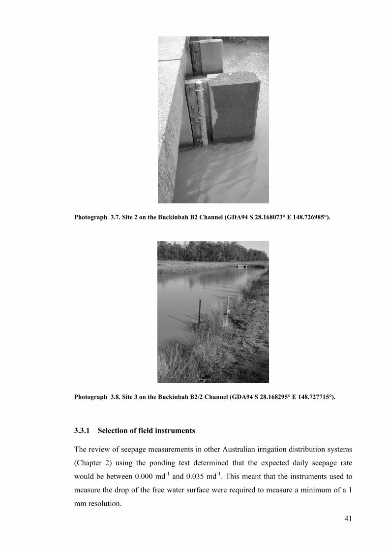
41
Photograph 3.7. Site 2 on the Buckinbah B2 Channel (GDA94 S 28.168073° E 148.726985°).
Photograph 3.8. Site 3 on the Buckinbah B2/2 Channel (GDA94 S 28.168295° E 148.727715°).
3.3.1 Selection of field instruments
The review of seepage measurements in other Australian irrigation distribution systems
(Chapter 2) using the ponding test determined that the expected daily seepage rate
would be between 0.000 md-1
and 0.035 md-1
. This meant that the instruments used to
measure the drop of the free water surface were required to measure a minimum of a 1
mm resolution.
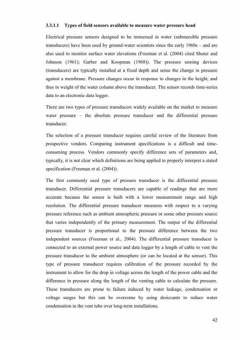
42
3.3.1.1 Types of field sensors available to measure water pressure head
Electrical pressure sensors designed to be immersed in water (submersible pressure
transducers) have been used by ground-water scientists since the early 1960s – and are
also used to monitor surface water elevations (Freeman et al. (2004) cited Shuter and
Johnson (1961); Garber and Koopman (1968)). The pressure sensing devices
(transducers) are typically installed at a fixed depth and sense the change in pressure
against a membrane. Pressure changes occur in response to changes in the height, and
thus in weight of the water column above the transducer. The sensor records time-series
data to an electronic data logger.
There are two types of pressure transducers widely available on the market to measure
water pressure – the absolute pressure transducer and the differential pressure
transducer.
The selection of a pressure transducer requires careful review of the literature from
prospective vendors. Comparing instrument specifications is a difficult and time-
consuming process. Vendors commonly specify difference sets of parameters and,
typically, it is not clear which definitions are being applied to properly interpret a stated
specification (Freeman et al. (2004)).
The first commonly used type of pressure transducer is the differential pressure
transducer. Differential pressure transducers are capable of readings that are more
accurate because the sensor is built with a lower measurement range and high
resolution. The differential pressure transducer measures with respect to a varying
pressure reference such as ambient atmospheric pressure or some other pressure source
that varies independently of the primary measurement. The output of the differential
pressure transducer is proportional to the pressure difference between the two
independent sources (Freeman et al., 2004). The differential pressure transducer is
connected to an external power source and data logger by a length of cable to vent the
pressure transducer to the ambient atmosphere (or can be located at the sensor). This
type of pressure transducer requires calibration of the pressure recorded by the
instrument to allow for the drop in voltage across the length of the power cable and the
difference in pressure along the length of the venting cable to calculate the pressure.
These transducers are prone to failure induced by water leakage, condensation or
voltage surges but this can be overcome by using desiccants to reduce water
condensation in the vent tube over long-term installations.

43
The second commonly used type of pressure transducer is the absolute pressure
transducer. The absolute pressure sensor measures the water pressure, as well as, the air
pressure pushing on the water surface – so, if the air pressure varies, the measured water
pressure will also vary, without having to vary the water level (Schlumberger Water
Services, 2014). Absolute pressure is measured in reference to a vacuum or zero
pressure – (pressure at sea level is 101.3 kPa) and pressures measured by an absolute
pressure transducer are always positive because these devices are referenced to a perfect
vacuum in which absolute pressure is zero (Dunn, 2010).
The main advantage of the absolute pressure transducer over the differential pressure
transducer is that it is an all-in-one unit, which includes a power supply housed with the
pressure membrane and data logger, so additional field equipment and calibration is
reduced, e.g. wiring and placement of power supply, cabling and housing. The main
disadvantage of the absolute pressure transducer is that the membrane can be more
sensitive to temperature changes and the pressure value recorded includes the
atmospheric pressure acting on the sensor. A second pressure transducer measuring the
atmospheric pressure must be used to calculate the water pressure head and this value is
subtracted from the absolute pressure reading – which introduces a potential instrument
error in the final pressure calculation.
Although two field measurement units are required to measure water pressure with the
absolute pressure sensor it can be programmed by the user to return a raw pressure
value which is already calibrated by the vendor. The absolute pressure sensor requires
smaller housing in the field and is easily deployed because no auxiliary power supplies
are required.
The second pressure transducer used to measure the on-site barometric pressure is used
to compensate for the difference in the absolute water pressure with the barometric
pressure. These transducers are also not prone to failure induced by water leakage or
voltage surges, as they are a completely sealed unit.
The absolute pressure transducer was selected for this study to measure the water
pressure and temperature of the water during the ponding tests based on availability and
ease of deployment.

44
3.3.1.2 Minimum measurement parameters and accuracy of the field
measurements
This study used two measurements to estimate the daily seepage rate at three sites.
The first source of measurement was the pressure sensor measuring the water level in
the channel. The second source of measurement was the daily evapotranspiration and
daily rainfall collated by the BoM automated weather station located at the St George
Airport.
The accuracy of the water level measurement was limited to the smallest resolution of
the pressure sensor shown previously in Table 3.2. The resolution of the pressure
sensors were:
- Site 1: St George Main Channel at the Beeson Road sites - 0.002 m
- Site 2: Buckinbah B2 Channel - 0.001 m
- Site 3: Buckinbah B2/2 Channel - 0.001 m.
The accuracy of the daily evapotranspiration and daily rainfall reported by the BoM was
five significant figures, e.g. 0.0048 m. The daily evapotranspiration data was more
readily available than pan evaporation data and the evapotranspiration data was used in
place of evaporation data (discussed later in Chapter 4). Evaporation is spatially less
variable than rainfall and so the 20 km distance between the field installations and the St
George Airport provided adequate accuracy.
3.3.1.3 Field installation and deployment of the pressure sensors
The pressure sensors measured the change of the water depth in the water supply
channel and were housed inside a steel conduit and anchored to the channel
embankment (Photograph 3.5). The steel conduit acted as a stilling well to protect the
logger from vibration, shock and movement, including current, wave action and debris
as recommended by the manufacturer product manual.
Where possible, the installation located the pressure sensors as near as possible to the
deepest part of the channel, i.e. the bed of the channel at the toe of the internal channel
embankment so that the logger reading could be calibrated by manual measurement.

45
The pressure sensor was secured to a length of small diameter PVC conduit and inserted
in the larger diameter steel conduit. A concrete plate was placed under the toe of the
steel conduit to reduce the distance the conduit settled into the silted channel during the
installation.
This installation configuration improved safe access to the pressure sensor as the
operator could stand on the bank of the channel to access the pressure sensor without
entering the water body. The main advantage was the elimination of the hazard of a
person entering the water to recover the instrument from the channel. It also allowed for
careful placement of the sensor and protected the instrument from shock.
The manufacturer recommended the sensor was oriented in the vertical, however, in this
study the steel conduit was anchored down a sloped bank, leaving the transducer
oriented out of vertical on the diagonal. Therefore, to reduce the drift (potentially
caused by the rise and fall in of the water in the steel conduit) of the reference datum for
the membrane housed inside the pressure sensor it was secured to a length of PVC
conduit inserted inside the steel conduit. The manufacturer of the Onset HOBO logger
advised the device would work equally well horizontally or vertically provided the
pressure pore was not impeded (Onset, 2015).
The reference water level recorded by the pressure sensor was calibrated by an
independent manual measurement of the water level in the channel following each
deployment.
To achieve the best level of accuracy from the pressure sensors, the HOBO product
manual recommended sudden temperature change should be avoided and some
consideration should be made to minimise the rate of temperature fluctuations. Ideally,
the barometric pressure reference logger should be hung several feet below ground level
in an observation well where ground temperatures are stable or if this is not possible, to
put the logger in a location where it will not be subject to rapid daily temperature
cycles.
In this study, the pressure sensors were housed in steel tubing, which absorbed and
released the heat caused by temperature fluctuations. The data recorded has been
analysed carefully to account for this known environmental factor (as discussed in
Chapter 4).

46
3.4 Seepage calculation
This section details the ponding test procedure previously introduced in section 2.3.2.
The principle measurement method used in this study was the ponding test. The
ponding test used a water balance to determine seepage losses in an isolated reach of a
channel. The ponded length of channel was isolated using existing check structures.
Seepage losses constitute the drop in water level over time in the pond after accounting
for evaporation, rainfall and any other inflows or outflows. As the water level in the
ponded channel section dropped, the pressure sensor measured the water level. The time
between measurements was set to hourly increments during the logger setup. Daily
rainfall and evapotranspiration data was collected by the nearby BoM automated
weather station located at the St George Airport, and the resulting seepage loss rate was
computed (using the equation introduced later in section 3.4.3).
3.4.1 Channel geometry used to estimate the volumetric losses
The As Built Drawings (DNR, 1998, Irrigation and Water Supply Commission
Queensland, 1972a, Irrigation and Water Supply Commission Queensland, 1972b)
(Appendix C) of the longitudinal cross sections of Site 1: St George Main Channel, Site
2: Buckinbah B2 Channel and Site 3: Buckinbah B2/2 Channel were used to calculate
the channel capacity and geometric relationships for each channel section.
The operating depth was used to calculate the surface area of the water body in the
channel and the area of the wetted perimeter of the channel below the water surface.
The calculated surface areas at the operating depth were used to estimate the daily
volume of water losses in the channel to seepage.
3.4.2 Monitoring parameters during the test
The three parameters monitored during the ponding test were the water level,
evapotranspiration and the rainfall.
The Best Practice Guidelines for Channel Seepage Identification and Measurement by
SKM (2003) recommended that water level, evapotranspiration and rainfall should be
taken daily. To increase the available data and monitor instrument error the water levels
were recorded hourly. The Bureau of Meteorology reported evapotranspiration on a
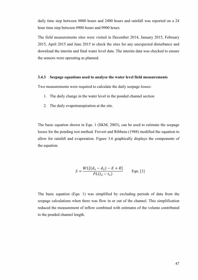
47
daily time step between 0000 hours and 2400 hours and rainfall was reported on a 24
hour time step between 0900 hours and 0900 hours.
The field measurements sites were visited in December 2014, January 2015, February
2015, April 2015 and June 2015 to check the sites for any unexpected disturbance and
download the interim and final water level data. The interim data was checked to ensure
the sensors were operating as planned.
3.4.3 Seepage equations used to analyse the water level field measurements
Two measurements were required to calculate the daily seepage losses:
1. The daily change in the water level in the ponded channel section
2. The daily evapotranspiration at the site.
The basic equation shown in Eqn. 1 (SKM, 2003), can be used to estimate the seepage
losses for the ponding test method. Frevert and Ribbens (1988) modified the equation to
allow for rainfall and evaporation. Figure 3.6 graphically displays the components of
the equation.
𝑆 = 𝑊𝐿[(𝑑1 − 𝑑2) − 𝐸 + 𝑅]𝑃𝐿(𝑡2 − 𝑡1)
Eqn. [1]
The basic equation (Eqn. 1) was simplified by excluding periods of data from the
seepage calculations when there was flow in or out of the channel. This simplification
reduced the measurement of inflow combined with estimates of the volume contributed
to the ponded channel length.
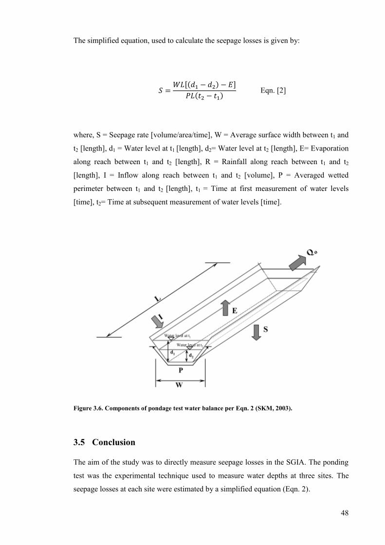
48
The simplified equation, used to calculate the seepage losses is given by:
𝑆 = 𝑊𝐿[(𝑑1 − 𝑑2) − 𝐸]𝑃𝐿(𝑡2 − 𝑡1)
Eqn. [2]
where, S = Seepage rate [volume/area/time], W = Average surface width between t1 and
t2 [length], d1 = Water level at t1 [length], d2= Water level at t2 [length], E= Evaporation
along reach between t1 and t2 [length], R = Rainfall along reach between t1 and t2
[length], I = Inflow along reach between t1 and t2 [volume], P = Averaged wetted
perimeter between t1 and t2 [length], t1 = Time at first measurement of water levels
[time], t2= Time at subsequent measurement of water levels [time].
Figure 3.6. Components of pondage test water balance per Eqn. 2 (SKM, 2003).
3.5 Conclusion
The aim of the study was to directly measure seepage losses in the SGIA. The ponding
test was the experimental technique used to measure water depths at three sites. The
seepage losses at each site were estimated by a simplified equation (Eqn. 2).

49
The measurement sites were selected due to supply capacity, soil types and channel
construction methods. Site 1: (The St George Main Channel) was a clay lined channel
constructed in low water-holding capacity soils. Site 2: (Buckinbah B2 Channel) and
Site 3: (Buckinbah B2/2 Channel) were constructed using compacted earth in sandy
soils.
The water depths in the isolated channel sections were measured using absolute pressure
sensors housed in stilling wells. The ponded length of channel was isolated using
existing check structures. The channels were in operation during the ponding tests.
Chapter 4 follows to present and discuss the results of the ponding tests.

50
Chapter 4 Experimental results and discussion
This chapter presents the results of the water depth data collected using the techniques
and equipment described in Chapter 3. The water depth data and evapotranspiration data
were collected to measure the seepage losses described in Chapter 1.
The aim of the study was to develop an estimate of seepage loss in the SGIA by
interpreting the daily water level data measured using the ponding test. Where seepage
losses were identified the results were compared against the results of the other studies
of seepage losses (Table 2.4).
Chapter 2 reviewed Australian studies of seepage loss and the estimates for a variety of
soils and channel linings were between 0.000 md-1
and 0.070 md-1
. The predicted
seepage losses for the study area were between 0.000 md-1
and 0.015 md-1
.
The analysis presented demonstrates the potential for improving the water level
measurement technique (outlined in Chapter 3) used during the ponding test.
The data trends were processed using the steps shown in Figure 4.1.
Figure 4.1. The seepage losses were estimated using data that suggested the falling water depth was due to seepage alone.
4.1 Experimental measurement
Two measurements were collected to estimate the daily seepage losses:
1. The daily water head in the ponded channel section
2. The daily rainfall and evapotranspiration measured by the automated weather
station located at the St George Airport.
The pressure sensors described in Chapter 3 were used to measure the water head
(depth) in the channel at three sites. The HOBOware software and Schlumberger Diver
Water Head Data Trend
Analyse Daily Depth
Trend
Estimate Seepage
Loss
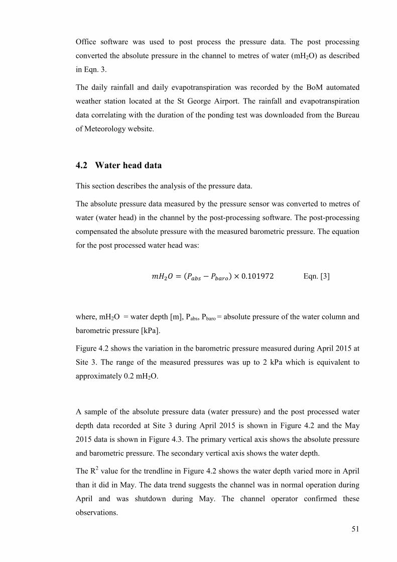
51
Office software was used to post process the pressure data. The post processing
converted the absolute pressure in the channel to metres of water (mH2O) as described
in Eqn. 3.
The daily rainfall and daily evapotranspiration was recorded by the BoM automated
weather station located at the St George Airport. The rainfall and evapotranspiration
data correlating with the duration of the ponding test was downloaded from the Bureau
of Meteorology website.
4.2 Water head data
This section describes the analysis of the pressure data.
The absolute pressure data measured by the pressure sensor was converted to metres of
water (water head) in the channel by the post-processing software. The post-processing
compensated the absolute pressure with the measured barometric pressure. The equation
for the post processed water head was:
𝑚𝐻2𝑂 = (𝑃𝑎𝑏𝑠 − 𝑃𝑏𝑎𝑟𝑜) × 0.101972 Eqn. [3]
where, mH2O = water depth [m], Pabs, Pbaro = absolute pressure of the water column and
barometric pressure [kPa].
Figure 4.2 shows the variation in the barometric pressure measured during April 2015 at
Site 3. The range of the measured pressures was up to 2 kPa which is equivalent to
approximately 0.2 mH2O.
A sample of the absolute pressure data (water pressure) and the post processed water
depth data recorded at Site 3 during April 2015 is shown in Figure 4.2 and the May
2015 data is shown in Figure 4.3. The primary vertical axis shows the absolute pressure
and barometric pressure. The secondary vertical axis shows the water depth.
The R2 value for the trendline in Figure 4.2 shows the water depth varied more in April
than it did in May. The data trend suggests the channel was in normal operation during
April and was shutdown during May. The channel operator confirmed these
observations.

52
Figure 4.2. The time series pressure data and water depth data at Site 3 [April 2015].
After it was confirmed that the channel was shutdown during May, the data was
analysed on a smaller daily timestep to identify data that suggested the falling water
depth trend was due to seepage losses.
To explain how the trend in the water depth data related to seepage loss was identified
during the data analysis the next section describes two data samples recorded over
smaller 24 hour periods during April and May 2015. The data samples were recorded
during:
1. Sample 1: Normal channel operation
2. Sample 2: Channel shutdown.
R² = 0.3819
0.5
0.6
0.7
0.8
9899
100101102103104105106107108
1 2 3 4 5 6 7 8 9 101112131415161718192021222324252627282930
Wat
er D
epth
[m]
Pres
sure
[kPa
]
Day
Logger Pressure Data and Water Depth B2/2 Channel [April 2015]
Water Pressure Barometric Pressure Water Depth Linear (Water Depth)

53
Figure 4.3. The time series pressure data and water depth data at Site 3 [May 2015].
4.2.1 Site 3: Sample data during normal channel operation
The post-processed water head data for 11 April 2015 is used to illustrate the typical
behaviour during channel shutdown where no inflows or outflows were occurring
(Figure 4.4). The data was recorded during normal channel operation. The primary
vertical axis shows the absolute pressure and barometric pressure. The secondary
vertical axis shows the water depth.
On 11 April 2015, the water depth started at 0.735 m at hour 1 and finished at 0.735 m
at hour 24. There was a slight rise in the water depth that coincided with a slight rise in
the barometric pressure at hour 10. A drop in the water depth followed the slight rise
during the middle of the day and after hour 16 the water depth rose again.
The expected trend in the post processed water head data was a smooth falling line over
each 24 hour period. As can be seen in Figure 4.4 the water depth did not fall smoothly
over the 24 hour period. The trend line for the processed water depth was a poor fit with
an R2 value of 0.0476.
R² = 0.835
0.5
0.6
0.7
0.8
9899
100101102103104105106107108
1 2 3 4 5 6 7 8 9 10111213141516171819202122232425262728293031
Wat
er D
epth
[m]
Pres
sure
[kPa
]
Day
Logger Pressure Data and Water Depth B2/2 Channel [May 2015]
Water Pressure Barometric Pressure Water Depth Linear (Water Depth)
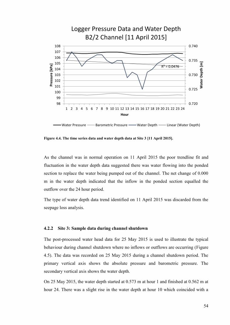
54
Figure 4.4. The time series data and water depth data at Site 3 [11 April 2015].
As the channel was in normal operation on 11 April 2015 the poor trendline fit and
fluctuation in the water depth data suggested there was water flowing into the ponded
section to replace the water being pumped out of the channel. The net change of 0.000
m in the water depth indicated that the inflow in the ponded section equalled the
outflow over the 24 hour period.
The type of water depth data trend identified on 11 April 2015 was discarded from the
seepage loss analysis.
4.2.2 Site 3: Sample data during channel shutdown
The post-processed water head data for 25 May 2015 is used to illustrate the typical
behaviour during channel shutdown where no inflows or outflows are occurring (Figure
4.5). The data was recorded on 25 May 2015 during a channel shutdown period. The
primary vertical axis shows the absolute pressure and barometric pressure. The
secondary vertical axis shows the water depth.
On 25 May 2015, the water depth started at 0.573 m at hour 1 and finished at 0.562 m at
hour 24. There was a slight rise in the water depth at hour 10 which coincided with a
R² = 0.0476
0.720
0.725
0.730
0.735
0.740
9899
100101102103104105106107108
1 2 3 4 5 6 7 8 9 10 11 12 13 14 15 16 17 18 19 20 21 22 23 24
Wat
er D
epth
[m]
Pres
sure
[kPa
]
Hour
Logger Pressure Data and Water Depth B2/2 Channel [11 April 2015]
Water Pressure Barometric Pressure Water Depth Linear (Water Depth)
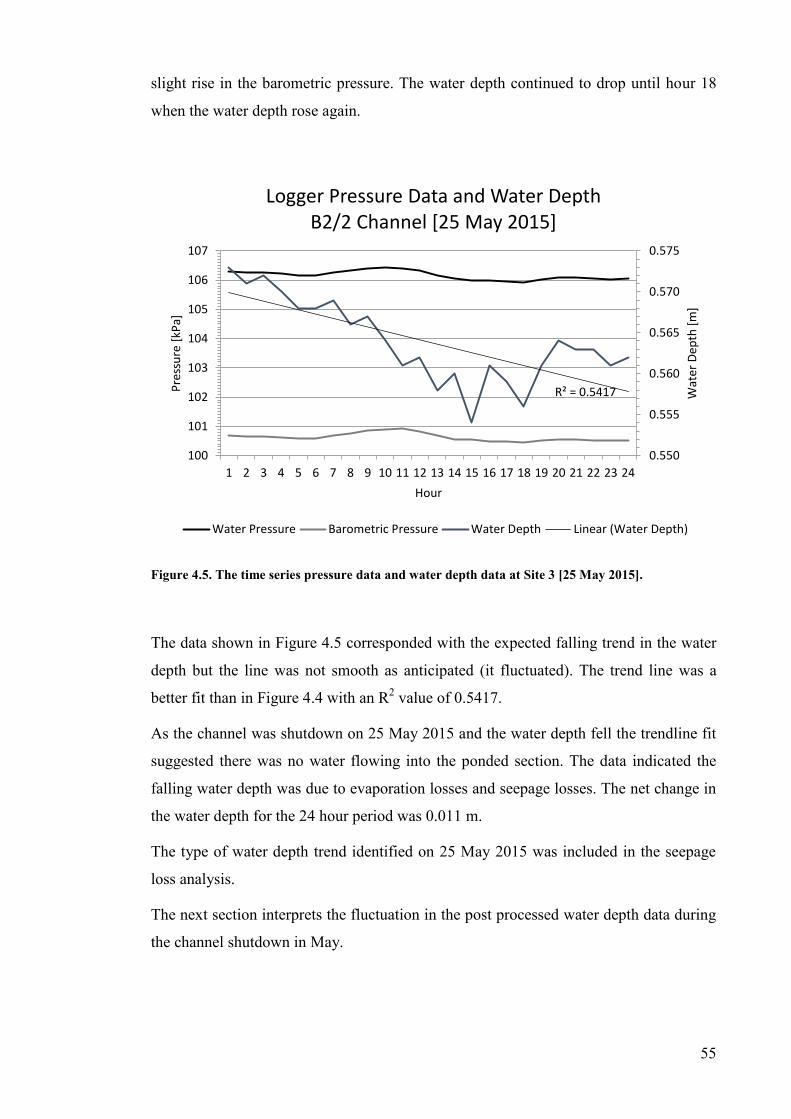
55
slight rise in the barometric pressure. The water depth continued to drop until hour 18
when the water depth rose again.
Figure 4.5. The time series pressure data and water depth data at Site 3 [25 May 2015].
The data shown in Figure 4.5 corresponded with the expected falling trend in the water
depth but the line was not smooth as anticipated (it fluctuated). The trend line was a
better fit than in Figure 4.4 with an R2 value of 0.5417.
As the channel was shutdown on 25 May 2015 and the water depth fell the trendline fit
suggested there was no water flowing into the ponded section. The data indicated the
falling water depth was due to evaporation losses and seepage losses. The net change in
the water depth for the 24 hour period was 0.011 m.
The type of water depth trend identified on 25 May 2015 was included in the seepage
loss analysis.
The next section interprets the fluctuation in the post processed water depth data during
the channel shutdown in May.
R² = 0.5417
0.550
0.555
0.560
0.565
0.570
0.575
100
101
102
103
104
105
106
107
1 2 3 4 5 6 7 8 9 10 11 12 13 14 15 16 17 18 19 20 21 22 23 24
Wat
er D
epth
[m]
Pres
sure
[kPa
]
Hour
Logger Pressure Data and Water Depth B2/2 Channel [25 May 2015]
Water Pressure Barometric Pressure Water Depth Linear (Water Depth)
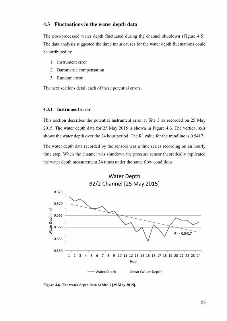
56
4.3 Fluctuations in the water depth data
The post-processed water depth fluctuated during the channel shutdown (Figure 4.5).
The data analysis suggested the three main causes for the water depth fluctuations could
be attributed to:
1. Instrument error
2. Barometric compensation
3. Random error.
The next sections detail each of these potential errors.
4.3.1 Instrument error
This section describes the potential instrument error at Site 3 as recorded on 25 May
2015. The water depth data for 25 May 2015 is shown in Figure 4.6. The vertical axis
shows the water depth over the 24 hour period. The R2 value for the trendline is 0.5417.
The water depth data recorded by the sensors was a time series recording on an hourly
time step. When the channel was shutdown the pressure sensor theoretically replicated
the water depth measurement 24 times under the same flow conditions.
Figure 4.6. The water depth data at Site 3 [25 May 2015].
R² = 0.5417
0.550
0.555
0.560
0.565
0.570
0.575
1 2 3 4 5 6 7 8 9 10 11 12 13 14 15 16 17 18 19 20 21 22 23 24
Wat
er D
epth
[m]
Hour
Water Depth B2/2 Channel [25 May 2015]
Water Depth Linear (Water Depth)

57
The accuracy of the water depth data at Site 3 was ± 0.003 m. The resolution of the
water depth data at Site 3 was 0.001 m. This meant that between each time step there
was a potential instrument error of ± 0.003 m.
When the channel was shutdown the daily water depth data in the channel was expected
to drop by a depth of up to 0.015 m due to evaporation and seepage water losses. The
hourly water depths are shown in Table 4.1. The data shows the water depth fluctuated
between hourly measurements by up to 0.007 m which was greater than the potential
instrument error (discussed later in section 4.3.2).
The change in the water depth was within the potential instrument error of ± 0.003 m
between hour 1 and hour 11 and again from hour 18 until hour 24. The instrument error
range suggested the true value for the water depth was more likely to be replicated when
the hourly water depths varied between ± 0.003 m of the previous value.
Table 4.1. Hourly water depth data at Site 3 [25 May 2015].
Hour Water Depth [m] Change from Previous Hour [m]
1 0.573 0.000
2 0.571 0.002
3 0.572 -0.001
4 0.570 0.002
5 0.568 0.002
6 0.568 0
7 0.569 -0.001
8 0.566 0.003
9 0.567 -0.001
10 0.564 0.003
11 0.561 0.003
12 0.562 -0.001
13 0.558 0.004
14 0.560 -0.002
15 0.554 0.006
16 0.561 -0.007
17 0.559 0.002
18 0.556 0.003
19 0.561 -0.005
20 0.564 -0.003
21 0.563 0.001
22 0.563 0
23 0.561 0.002
24 0.562 -0.001
58
During the first 11 hours, the water depth of 0.568 m was replicated by the sensor two
times at hour 4 and at hour 5. Over the entire 24 hour period the water depth of 0.561 m
was replicated by the sensor four times at hour 10, hour 15, hour 18 and hour 22.
The replication of the data indicated the true value at the start of the 24 hour period was
0.568 m and the true value at the end of the 24 hour period was 0.561 m. This analysis
suggested the water depth dropped by 0.007 m on 25 May 2015 due to evaporation and
seepage losses.
To add further confidence in the data - the water depth of 0.568 m was replicated at the
end of the data on the previous day, 24 May 2015. Further, the water depth of 0.561 m
was replicated at the beginning of the following day, 26 May 2015.
The data analysis showed the water depth fluctuated between readings by values greater
than the instrument error. Nonetheless, the instrument replicated water depth values
while producing water depth within the range of the instrument error. In conclusion, the
water depth data suggested the replicated readings were the true values for the water
depths.
The next sections suggest an explanation for the fluctuation in the water depth that were
greater than the instrument error of ± 0.003 m.
4.3.2 Barometric compensation calculation
The barometric pressure was subtracted from the absolute pressure measured in the
channel to convert the pressure readings to metres of water (mH2O). The barometric
pressure sensor and the absolute pressure sensor were located nearby each other to
reduce the spatial variation in barometric pressure readings. The barometric
compensation equation was shown earlier in this chapter as:
𝑚𝐻2𝑂 = (𝑃𝑎𝑏𝑠 − 𝑃𝑏𝑎𝑟𝑜) × 0.101972 Eqn. [4]
where, mH2O = water depth [m], Pabs, Pbaro = absolute pressure of the water column and
barometric pressure [kPa].

59
It can be seen from the Eqn. 4 that a slight fluctuation in the barometric pressure may
have a significant effect on the calculated water depth (mH2O); even though the
absolute pressure in the channel may not have varied. Hence, a slight fluctuation in
barometric pressure may explain a sudden change in the estimated water depth that was
outside the range of the instrument error of ± 0.003 m (e.g. hour 16 and hour 17 as
shown in Table 4.1).
The absolute pressure and barometric pressures logged on 25 May 2015 are shown in
Figure 4.7 and the data is shown in Table 4.2. The vertical axis shows the pressure
reading and the horizontal axis shows the hour the pressure was recorded.
Figure 4.7. The absolute pressure data and barometric data at Site 3 [25 May 2015].
100.00
101.00
102.00
103.00
104.00
105.00
106.00
107.00
1 2 3 4 5 6 7 8 9 10 11 12 13 14 15 16 17 18 19 20 21 22 23 24
Pres
sure
[kPa
]
Hour
Pressure Readings B2/2 Channel [25 May 2015]
Absolute Pressure Barometric Pressure

60
The data in Table 4.2 shows the absolute pressure of the water column in the channel
and the absolute pressure of the atmosphere (barometric). The water pressure was
calculated by subtracting the barometric pressure from the absolute pressure (Eqn. 3).
The water pressure in kPa was then multiplied by 0.101972 to convert the water
pressure to water depth (mH2O). The last column in Table 4.2 shows the difference in
the water pressure between each hourly reading.
Table 4.2. Hourly pressure depth comparison data at Site 3 [25 May 2015].
Hour Abs Pres [kPa] Abs Pres Barom [kPa] Water Pres[kPa] Difference in Hourly Water Pres [kPa]
1 106.30 100.68 5.62 -
2 106.27 100.67 5.60 0.03
3 106.25 100.64 5.61 -0.02
4 106.21 100.62 5.59 0.02
5 106.17 100.60 5.57 0.02
6 106.16 100.60 5.57 0.00
7 106.27 100.69 5.58 -0.01
8 106.32 100.76 5.55 0.03
9 106.41 100.85 5.56 -0.01
10 106.43 100.90 5.53 0.04
11 106.41 100.91 5.50 0.03
12 106.33 100.81 5.52 -0.02
13 106.16 100.68 5.48 0.04
14 106.05 100.56 5.49 -0.01
15 105.99 100.55 5.44 0.05
16 105.99 100.48 5.51 -0.07
17 105.95 100.47 5.48 0.03
18 105.90 100.45 5.46 0.02
19 106.03 100.52 5.51 -0.05
20 106.09 100.57 5.53 -0.02
21 106.09 100.56 5.52 0.00
22 106.06 100.54 5.53 0.00
23 106.03 100.53 5.50 0.03
24 106.04 100.53 5.51 -0.01
The barometric pressure change between hours on 25 May 2015 ranged between 0 kPa
and 0.07 kPa. The largest fluctuations in barometric pressure was between hour 15 (0.05
kPa) to hour 16 (0.07 kPa) and at hour 19 (0.05 kPa). At the same time, the change in
the water depth was greater than the instrument error of ± 0.003 m. The analysis of the
fluctuation in the barometric pressure indicated that when the channel was shutdown
that fluctuating water depth changes could be explained by the barometric compensation
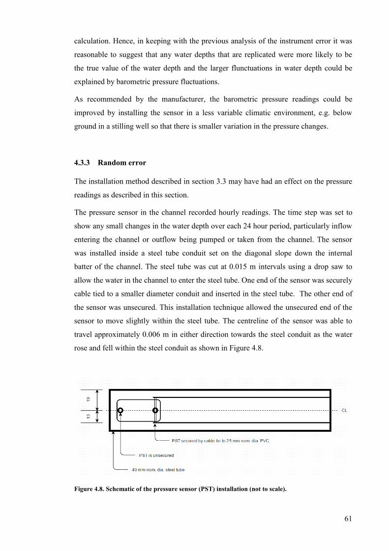
61
calculation. Hence, in keeping with the previous analysis of the instrument error it was
reasonable to suggest that any water depths that are replicated were more likely to be
the true value of the water depth and the larger flunctuations in water depth could be
explained by barometric pressure fluctuations.
As recommended by the manufacturer, the barometric pressure readings could be
improved by installing the sensor in a less variable climatic environment, e.g. below
ground in a stilling well so that there is smaller variation in the pressure changes.
4.3.3 Random error
The installation method described in section 3.3 may have had an effect on the pressure
readings as described in this section.
The pressure sensor in the channel recorded hourly readings. The time step was set to
show any small changes in the water depth over each 24 hour period, particularly inflow
entering the channel or outflow being pumped or taken from the channel. The sensor
was installed inside a steel tube conduit set on the diagonal slope down the internal
batter of the channel. The steel tube was cut at 0.015 m intervals using a drop saw to
allow the water in the channel to enter the steel tube. One end of the sensor was securely
cable tied to a smaller diameter conduit and inserted in the steel tube. The other end of
the sensor was unsecured. This installation technique allowed the unsecured end of the
sensor to move slightly within the steel tube. The centreline of the sensor was able to
travel approximately 0.006 m in either direction towards the steel conduit as the water
rose and fell within the steel conduit as shown in Figure 4.8.
Figure 4.8. Schematic of the pressure sensor (PST) installation (not to scale).
62
The fluctuation in the water depth data in the 25 May 2015 data sample was largely
attributed to the instrument error and barometric compensation described in the previous
sections. When there was a fluctuation that was not attributed to instrument error or
barometric compensation it was possible the error was random due to the installation
technique.
The installation technique could be improved by securing the both each of the sensor so
that the sensor cannot move within the steel tube.
The water depth data was analysed to reduce the errors as explained in this section. The
next section compares the difference between evapotranspiration data and evaporation
from open water.
4.4 Evapotranspiration and rainfall data
The second set of measurements used to estimate the daily seepage loss was the daily
evapotranspiration and rainfall measured by the automated weather station located at the
St George Airport. The St George Airport is located less than 2 km from Site 1 and less
than 20 km from Site 2 and Site 3. The seepage loss equation was described in Chapter
3. The equation subtracts evaporation along the ponded channel section from the water
depth to estimate seepage loss.
This study used evapotranspiration reported by the BoM to replace evaporation data.
The reasons for using evapotranspiration data in place of evaporation data and the
difference between evapotranspiration data and evaporation data is described in the next
section.
4.4.1 Evapotranspiration data compared to evaporation data
Evapotranspiration is not the same as evaporation. Evapotranspiration is the term used
to describe the part of the water cycle that removes liquid water from an area with
vegetation and into the atmosphere by the processes of both transpiration and
evaporation. Evaporation occurs when liquid water is converted to water vapour and
hence removed from a surface, such as a lake, soil or wet vegetation, into the air. Daily
evaporation is generally greater than daily evapotranspiration. Evapotranspiration is
related to evaporation from an open water body (such as a channel) by a pan coefficient
(Allen et al., 1998).

63
There was no evaporation data published for the St George region so for this
comparative analysis the evaporation was calculated using the widely accepted Penman
evaporation equation as simplified by Valiantzas’ (2006) (Eqn. 5).
Valiantzas’ (2006) simplified equation was used because he cited the main disadvantage
of the original Penman evaporation equation was that the main weather variables
appearing directly in the equation were usually not readily available and the complexity
of the calculation can result in significant errors. Valiantzas’ simplified version of the
standardized Penman equation uses routine weather records usually available at
standard weather stations, i.e. air temperature, solar radiation, relative humidity, and
wind velocity.
The simplified equation for estimating open water evaporation (EOW) not requiring wind
speed data is:
𝐸𝑂𝑊 ≈ 0.047𝑅𝑆√𝑇 + 9.5 − 2.4 (𝑅𝑆𝑅𝐴)2+ 0.09(𝑇 + 20) (1 − 𝑅𝐻
100) Eqn. [5]
where, Rs = solar radiation [MJ/m2/d], RA = extraterrestrial radiation [MJ/m
2/d], T =
average temperature [°C], RH = relative humidity [%].
The empirical equation for the extraterrestrial radiation, RA is:
𝑅𝐴 ≈ 3𝑁 sin(0.131𝑁 − 0.2𝜙) Eqn. [6]
where, N = daylight hours [hours], ϕ is the latitude for the site [radians].
The empirical equation for the daylight hours, N is:
𝑁 ≈ 4𝜙 sin(0.53𝑖 − 1.65) + 12 Eqn. [7]
where, i = rank of the month (i.e. first month is January).
64
The calculation of the evaporation data (EOW) is shown in Table 4.3. The EOW results
were compared with the evapotranspiration BoM calculations by using a pan factor.
McJannet et al. (2008) discussed the use of pan factors to estimate open water
evaporation in channels in Tatura, Victoria. There are numerous coefficients reported in
the literature but the shortfall of the technique is that coefficients are specific to the pan
type, its location and the nature of the water body and so require calibration for
individual applications. The uncertainty in developing coefficients makes this approach
unattractive. However, when modelled in Tatura, the estimates to test the performance
of the evaporation estimates based on pan evaporation data held a good correlation
when a pan coefficient of 0.7 was used. Hence, a pan coefficient of 0.7 was applied to
the estimated open water evaporation calculated by the Valiantzas’ equation.
The estimated open water evaporation for May 2015 was calculated using the BoM
weather station data recorded at the St George Airport and the Valiantzas’ (2006)
simplified equation as shown in Table 4.3. Where, EOW = estimated evaporation open
water, ET = BoM evapotranspiration, Pan Factor = EOW x 0.7 and Difference = ET –
Pan Factor.
Table 4.3 shows the daily difference in the estimated open water evaporation
(multiplied by the pan factor) and the evapotranspiration published by BoM is less than
1 mm with an average difference of 0.1 mm.
Given the uncertainty of developing a calibrated open water evaporation pan coefficient
and the relationship between the factors outlined in Table 4.3 the evapotranspiration
data published by the BoM was used for this study.
Further, the BoM has studied the evaporation and evapotranspiration data, from seven
weather stations located within the Murray-Darling Basin over a 29 year period and
concluded that there was a strong positive correlation between daily evaporation and
daily evapotranspiration at all sites (Webb, 2010).
The BoM publishes a monthly review of climate data and trends as well as long-term
data for each weather station. The cumulative evapotranspiration measured during the
ponding tests was 207.4 m, which was below the long-term sum of the mean potential
monthly evapotranspiration for April and May.

65
Table 4.3. Comparison of open water evaporation and evapotranspiration [May 2015].
Day EOW [mm] ET [mm] Pan Factor [mm] Difference [mm]
1 1.7 1.7 1.2 0.5
2 3.1 2.1 2.1 0.0
3 4.7 3.5 3.3 0.2
4 5.4 3.4 3.8 -0.4
5 5.5 3.4 3.8 -0.4
6 5.4 3.7 3.8 -0.1
7 5.0 3.3 3.5 -0.2
8 4.7 3.0 3.3 -0.3
9 4.2 2.5 2.9 -0.4
10 4.7 3.0 3.3 -0.3
11 5.1 3.7 3.6 0.1
12 4.7 2.6 3.3 -0.7
13 3.7 3.4 2.6 0.8
14 4.6 3.5 3.2 0.3
15 4.6 2.6 3.2 -0.6
16 4.7 3.3 3.3 0.0
17 3.9 2.8 2.8 0.0
18 4.7 3.2 3.3 -0.1
19 4.0 2.8 2.8 0.0
20 3.9 3.4 2.8 0.6
21 1.4 1.2 1.0 0.2
22 2.9 2.0 2.0 0.0
23 4.2 2.6 2.9 -0.3
24 4.2 2.6 2.9 -0.3
25 4.4 2.8 3.0 -0.2
26 3.8 2.3 2.7 -0.4
27 4.3 2.3 3.0 -0.7
28 4.4 2.3 3.1 -0.8
29 4.6 3.4 3.2 0.2
30 4.5 3.0 3.2 -0.2
31 3.8 2.7 2.6 0.1
4.4.2 Rainfall data
Rainfall intensity and volume varies spatially. The Australian Rainfall & Runoff Guide
suggests that a small catchment is defined as being less than 4 km2. Site 1 was located
less than 2 km from the BoM St George Airport automated weather station, however,
Site 2 and Site 3 were located 18 km away from the automated weather station. The
approximate catchment size was 50 km2. Hence, the rainfall recorded at the St George
Airport was merely an indicator of rainfall within the catchment. Despite the spatial
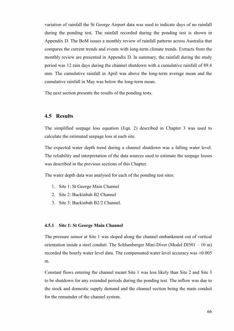
66
variation of rainfall the St George Airport data was used to indicate days of no rainfall
during the ponding test. The rainfall recorded during the ponding test is shown in
Appendix D. The BoM issues a monthly review of rainfall patterns across Australia that
compares the current trends and events with long-term climate trends. Extracts from the
monthly review are presented in Appendix D. In summary, the rainfall during the study
period was 12 rain days during the channel shutdown with a cumulative rainfall of 89.4
mm. The cumulative rainfall in April was above the long-term average mean and the
cumulative rainfall in May was below the long-term mean.
The next section presents the results of the ponding tests.
4.5 Results
The simplified seepage loss equation (Eqn. 2) described in Chapter 3 was used to
calculate the estimated seepage loss at each site.
The expected water depth trend during a channel shutdown was a falling water level.
The reliability and interpretation of the data sources used to estimate the seepage losses
was described in the previous sections of this Chapter.
The water depth data was analysed for each of the ponding test sites:
1. Site 1: St George Main Channel
2. Site 2: Buckinbah B2 Channel
3. Site 3: Buckinbah B2/2 Channel.
4.5.1 Site 1: St George Main Channel
The pressure sensor at Site 1 was sloped along the channel embankment out of vertical
orientation inside a steel conduit. The Schlumberger Mini-Diver (Model DI501 – 10 m)
recorded the hourly water level data. The compensated water level accuracy was ±0.005
m.
Constant flows entering the channel meant Site 1 was less likely than Site 2 and Site 3
to be shutdown for any extended periods during the ponding test. The inflow was due to
the stock and domestic supply demand and the channel section being the main conduit
for the remainder of the channel system.

67
Photograph 4.1 shows the gate structure at the end of the Site 1 ponded section
(Johnstone Road). There were a number of stock and domestic pump inlets supplied
from this section of the channel, which meant Site 1 was unlikely to be shutdown for
any extended periods.
Photograph 4.1. This photograph shows one of the 2 inch rural polyethylene pipeline pump inlets anchored in the channel to a length of white PVC in the Site 1 ponded section.
The water depth data was analysed over two periods recorded during April and May.
Figure 4.9 shows the water depth data measured at Site 1 during April 2015. The tabular
summary of the data is in Table E. 5. The primary vertical axis shows the change in the
water depth measured in the channel and the secondary vertical axis shows the water
losses due to evapotranspiration and seepage.
The data ranged between:
- Water depth [m]: 0.853 and 0.411 (0.442 m)
- Evapotranspiration [m]: 0.0055 and 0.0018 (0.0037 m).
There was a steady falling trend in the water depth between 4 April 2015 and 19 April
2015 (Figure 4.9). After 19 April 2015, there is a large inflow before normal operation
resumes at the end of the month. The chart shows the water depth at the beginning and
end of each 24-hour period. During this period the water depth was steadily falling,
however, closer examination of the hourly data showed there were inflows and outflows
from the channel during each 24-hour period.

68
The hourly water depth data (Figure 4.10) is used to illustrate the typical inflow and
outflow behaviour during each 24-hour period when the channel was in normal
operation. The data collected during normal channel operation was excluded from the
seepage loss analysis despite the steady falling trend in the 24-hour data (Figure 4.9).
The data was excluded due to the difficulty in separating the seepage losses and
evaporation losses from channel inflow and channel outflow and the resulting low
confidence in the calculated water depth data.
Figure 4.9. There were no periods during April 2015 where the falling water trend in the St George Main Channel was clearly due to seepage losses.
The combined analysis of the hourly water depth data and the 24-hour data (Figure 4.9)
indicated there were no periods during April 2015 when there were strong water depth
trends due to seepage losses. The hourly water depth data (Figure 4.10 and Figure 4.11)
showed constant inflow into the channel section and suggested there were no periods
when the channel section was shutdown.The tabular summary of the data is shown in
Table E.8a and Table E.8b.

69
Figure 4.10. The hourly water depth data shows there was water flowing into and out of the channel at Site 1 during the normal operation on 12 April 2015.
Figure 4.11. The hourly water depth data shows there was water flowing into and out of the channel at Site 1 during the normal operation on 13 April 2015.
0.500
0.505
0.510
0.515
0.520
0.525
0.530
0.535
1 2 3 4 5 6 7 8 9 10 11 12 13 14 15 16 17 18 19 20 21 22 23 24
Wat
er D
epth
[m]
Hour
Hourly Water Depth St George Main Channel [12 April 2015]
0.480
0.485
0.490
0.495
0.500
0.505
0.510
0.515
0.520
0.525
1 2 3 4 5 6 7 8 9 10 11 12 13 14 15 16 17 18 19 20 21 22 23 24
Wat
er D
epth
[m]
Hour
Hourly Water Depth St George Main Channel [13 April 2015]

70
Figure 4.12 shows the water depth data at Site 1 measured during May 2015. The
tabular summary of the data is in Table E. 6. The channel was in normal operation
during most of the month, with a large inflow around 9 May 2015 to maintain the
operating level.
The combined analysis of the hourly water depth data and the 24-hour data suggested
there were no periods during May 2015 when there was a strong water depth trend due
to seepage losses alone and the constant inflow and sharp outflow gradient suggested
there were no periods when the channel section was shutdown.
Figure 4.12. There were no periods when the water level dropped during May 2015 that were due to seepage losses and evaporation losses alone that could be separated from the channel flows.
4.5.2 Site 2: Buckinbah B2 Channel
The pressure sensor at Site 2 was in a vertical orientation inside a steel conduit anchored
to an abandoned culvert. A HOBO Water Level Logger (Model U20-001-04) recorded
the hourly water level data. The compensated water level accuracy was ±0.003 m. The
water depth data was analysed over two periods recorded during April and May.
Figure 4.13 shows the water depth data measured at Site 2 during April 2015. The
tabular summary of data is in Table E. 3. The primary vertical axis shows the water

71
depth measured in the channel and the secondary vertical axis shows the water losses
due to evapotranspiration and seepage.
There is a strong falling trend in the water between 9 April and 30 April, however, the
trend was the same as Site 1 and the combined analysis of the hourly water depth data
and the 24-hour data indicated there were no periods during April 2015 when there were
strong water level trends due to seepage losses. The water depth data indicated there
was constant inflow into the section during most of April or outflow due to water being
pumped from the channel.
The data ranged between:
- Water depth [m]: 0.376 and 0.284 (0.284 m)
- Evapotranspiration [m]: 0.0055 and 0.0018 (0.0037 m).
Figure 4.13. There were no periods during April 2015 where the falling water level trend in the B2 channel was due to seepage losses.
Figure 4.14 shows the water depth data measured at Site 2 during May 2015. The
tabular summary of the data shown in Figure 4.14 is in Table E. 4. The water depth was
below the pressure sensor during some of the ponding test. The analysis indicated there
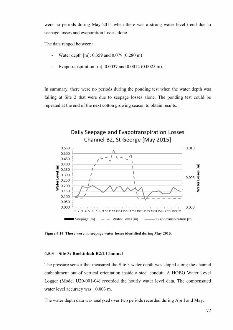
72
were no periods during May 2015 when there was a strong water level trend due to
seepage losses and evaporation losses alone.
The data ranged between:
- Water depth [m]: 0.359 and 0.079 (0.280 m)
- Evapotranspiration [m]: 0.0037 and 0.0012 (0.0025 m).
In summary, there were no periods during the ponding test when the water depth was
falling at Site 2 that were due to seepage losses alone. The ponding test could be
repeated at the end of the next cotton growing season to obtain results.
Figure 4.14. There were no seepage water losses identified during May 2015.
4.5.3 Site 3: Buckinbah B2/2 Channel
The pressure sensor that measured the Site 3 water depth was sloped along the channel
embankment out of vertical orientation inside a steel conduit. A HOBO Water Level
Logger (Model U20-001-04) recorded the hourly water level data. The compensated
water level accuracy was ±0.003 m.
The water depth data was analysed over two periods recorded during April and May.

73
Figure 4.15 shows the water depth data measured during April 2015 plotted as a line on
the primary vertical axis and the water losses plotted as a line on the secondary vertical
axis. The water depth data shows a steady fall in the water level between 1 April 2015
and 30 April 2015. The tabular summary of data shown in Figure 4.15 is in Table E. 1.
Despite the overall falling water level trend, the operator advised the channel was
operating during most of April 2015. The data analysis suggested water was being
pumped from the channel during the later stages of the month.
On days where there was potential seepage loss (at the end of April), the measured
water level fall was less than or equal to the water loss to evapotranspiration.
Subsequently, the same as at Site 1 and Site 2, the combined analysis of the hourly
water depth data and the 24-hour water depth data indicated there were no days in April
2015 when the falling water level was due to seepage losses and evaporation losses
alone.
Figure 4.15. The B2/2 Channel was is operation during April 2015 and the falling water level was equal to or less than the daily evapotranspiration recorded by the BoM automated weather station.
Figure 4.16 shows the water depth data measured at Site 3 during May 2015 plotted on
the primary vertical axis as a line. The secondary vertical axis shows the water losses;
the evapotranspiration loss is plotted in grey as a line and the seepage loss is plotted in
black as a column. There were 10 days between 19 May 2015 and 29 May 2015 when
74
the data indicated the falling water level was due to evapotranspiration and seepage
losses alone.
The data ranged between:
- Water depth [m]: 1.091 and 0.942 (0.149 m)
- Evapotranspiration [m]: 0.0012 and 0.0037 (0.0025 m)
- Seepage loss [m]: 0.004 and 0.013 (0.009 m).
Figure 4.16. There were 10 days of data during the shutdown in May 2015 where the seepage losses were estimated to be 0.008 md-1 ± 0.002 m (95 %).
These seepage losses were within the expected range of up to 0.015 m. The tabular
summary of data shown in Figure 4.16 is in Table E. 2. The seepage losses were
estimated to be 0.008 md-1
± 0.002 m (95 %) or in other words the true mean was
estimated to be within the range of 0.006 m and 0.010 m with a standard deviation of
0.002 m.
The As Built Drawings were used to calculate the water surface area and wetted
perimeter of the channel at the designed operating levels. These parameters were used to
estimate the annual losses due to seepage.

75
The wetted perimeter of the Buckinbah B2/2 Channel at the designed operating level
was 11100 m2. By extrapolation, a daily seepage loss of 0.008 md
-1 equates to an annual
loss of 32.5 ML.
The surface area of the Buckinbah B2/2 Channel at the designed operating level was
13900 m2. By using, an annual evaporation loss published from the Monthly
Evaporation Calculator (NCEA) of 2.485 m and the surface area of the B2/2 Channel,
the estimated annual loss to evaporation was 34.5 ML.
The Buckinbah B2/2 Channel supplies one SunWater customer 640 MLy-1
. Assuming
water was supplied between August and March only, the losses to seepage and
evaporation in the Buckinbah B2/2 Channel alone were approximately 10 per cent of
the total water released from Beardmore Dam as shown in Figure 4.17. There would be
additional losses to seepage and evaporation between the actual release point at the dam
and the following Thuraggi Channel, Buckinbah Main and B2/2 Channel (Figure 2.3).
Figure 4.17. The water losses in the Buckinbah B2/2 Channel alone during one irrigation season was approximately 10 per cent of the 640 ML of water released from Beardmore Dam.
There are approximately 14 km of earth channel between the Buckinbah Weir and the
offtake to the Buckinbah B2/2 Channel. By extrapolation, a daily seepage loss of 0.008
Total 90%
Evaporation loss 5%
Seepage loss 5%
Water delivery efficiency Buckinbah B2/2 Channel

76
md-1
equates to an annual loss of 365 ML and 295 ML annual loss to evaporation before
the water reaches the Buckinbah B2/2 Channel.
These losses would be distributed among all of the SunWater customers supplied by the
Buckinbah Channel system (supply capacity of 490 MLd-1
).
In summary, there was one period during the ponding test when the water depth was
falling at Site 3 that was due to seepage losses alone. The data suggested the daily
seepage loss was 0.008 md-1
± 0.002 m (95 %), which is approximately 5 per cent of the
water supplied to the Buckinbah B2/2 Channel annually.
4.6 Conclusion and review of results
The aim of the study was to develop an estimate of seepage loss in the SGIA by
interpreting the daily water level data measured using the ponding test. Where seepage
losses were identified, the results of this study were compared against the results of
other studies of seepage losses.
The water depth trends at Site 1 and Site 2 suggested the channel section was not
shutdown during the ponding test due to either normal inflow or outflow conditions
from the ponded section. Subsequently, there were no periods during the ponding tests
at Site 1 and Site 2 that could be attributed to seepage losses alone. Seepage estimates
for Site 1 and Site 2 could be obtained by future ponding tests.
Unfortunately, the null result at Site 1 and Site 2 meant that the seepage in a clay lined
channel on a contrasting soil type could not be compared to the results obtained at Site
3. Fortunately, the soil properties at Site 2 are similar to Site 3 (although the hydraulic
properties are different – refer Table 3.1) and so the seepage losses at Site 2 are likely to
be in the same order as the results obtained at Site 3; although due to the larger supply
capacity they may be greater.
The results of the ponding test at Site 3 identified a falling water depth trend in the
ponded section. The ponded section at Site 3 was approximately 1.4 km long. The water
depth data measured the fall in the water surface located approximately 100 m from the
start of the ponded section. The results of the ponding test indicated water ponded in the
section was as anticipated, being lost to both, evaporation and seepage; however, the
results do not indicate the precise location of the losses. The precise location of the

77
losses may be able to be identified during the initial filling at the beginning of the next
irrigation season or by using other methods to assess seepage losses described in
Chapter 2. The water depth measurements could be refined by placing multiple sensors
in the ponded section or by placing a sensor at a more centralised location.
The water depth trends at Site 3 indicated the seepage losses were 0.008 md-1
± 0.002 m
(95%). The soil mapping for Site 3 indicated the soils were texture contrast soils
comprised of Tenosols, Sodosols and Vertosols. While Tenosols have a high
permeability, Sodosols and Vertosols have low permeability. Soil properties are
generally not homogeneous for the entire length of an earth structure such as a channel,
therefore, the seepage losses may be unevenly distributed along the length of the
channel according to the soil property and channel maintenance/condition of the earth
structure, e.g. erosion.
Other studies of seepage losses irrigation channels in Australia that used the ponding
test (ANCID, 2003, McLeod et al., 1990, Moavenshahidi et al., 2014) estimated seepage
losses between 0.000 md-1
and 0.035 md-1
. The studies do not indicate the soil
properties, however, the results of this study are within the range reported. The results
of this study also compare well with the seepage rates of typical linings of clay loam
and hardpan, soil lining (Figure 2.6) reported in the USA study by Sonnichsen (1993).
Chapter 2 reviewed the methods to measure seepage losses. The ponding test used in
this study is an accurate method to identify overall losses in a channel, however, results
do not provide the spatial variation of losses but only a bulk figure for seepage. Smaller
seepage hotspots are identified by more localised methods such as, reducing the length
of the ponded section, the Idaho Seepage Meter or Geophysical methods. A channel
lining inspection may also identify localised damage in the channel, e.g. erosion or
tunnelling in the embankments. Although, the ponding test results are the most accurate
means of measuring channel seepage, they may still underestimate seepage compared to
channel flowing conditions (ANCID, 2003).
The results of this study are from one irrigation season. The data analysis identified one
10 day period where the falling water depths measured at Site 3 were clearly attributed
to seepage losses. As with all good scientific experiments the ponding test should be
duplicated under the same conditions to test the repeatability of the results obtained by
this study.

78
The cost of the ponding tests was minimised during this study as existing check
structures were used to pond the test sections and the measurement equipment cost less
than $5000 AUD. Other costs incurred were travel to the measurement sites and hours
spent analysing the water depth data and compiling the results of the study.
This chapter presented the results of the ponding tests at three sites. The sources of data
and the accuracy of the data were described in detail, including a discussion of:
1. The possible reasons for the fluctuation in the water depth data
2. The justification for using evapotranspiration data to estimate open water
channel evaporation.
The analysis of the trend in the water depth data during a shutdown period could be
improved by logging pressure readings at a finer interval (e.g. 15 minutes) to increase
the replication of the water depth measurements. Secondly, the barometric pressure
recording could be improved by installing the logger in a stilling well below ground
level where the atmospheric pressure fluctuates less. The pressure sensor installation
could also be improved by securing both ends of the sensor so the sensor cannot move
within the steel tube as the water depth changes. The absolute pressure transducers
could also be replaced by more accurate differential pressure transducers described in
Chapter 2.
79
Chapter 5 Conclusion
This chapter summarises the results of the study and sets a plan for further work to
improve and extend the results of the study.
The study area was the earthen channel distribution system located in the St George
Irrigation Area (SGIA) (part of the St George Water Supply Scheme). The demand for
irrigation water in the SGIA is influenced by the annual rainfall and semi-arid nature of
the catchment. The channel system supplies water mainly for irrigated cotton and some
horticulture.
The efficiency of irrigation systems has come into focus as food security has been
coming back on the centre stage as a major challenge for future decades. Seepage losses
contribute to the efficiency of irrigation systems. Seepage in the dominant process by
which water is lost from earthen distribution channels, along with evaporation, which
can also contribute to a high proportion of losses in dry areas.
The accurate estimation of seepage losses is a concern when optimising water supply
operations in channel systems and investigating in infrastructure improvements. The
SGIA is an important economic region for agricultural production in the MDB.
Improving the knowledge of supply system losses, such as seepage, has the potential to
lead to better water efficiency within the channel system.
There are currently no published estimates of seepage losses in irrigation systems in
southwest Queensland. This study estimated the seepage losses in the SGIA by directly
measuring water depths and using the ponding test. The seepage rate is controlled
mainly by the effective hydraulic continuity of the underlying base material. The other
studies (Chapter 2) of seepage losses identified that seepage losses are estimated to be
up to 25 per cent of any release into a channel supply system. All of the other seepage
loss studies reviewed concluded that seepage losses reduced the efficiency of water
distribution. Seepage loss rates estimated in Australian channel systems using the
ponding test vary between 0.000 md-1
and 0.035 md-1
. The results of seepage estimates
can be affected by seasonal variation. The IQQM computer simulation of the SGIA
currently uses a loss factor of 1.15 to estimate the operational efficiency of water
delivered to SunWater customers.
Chapter 3 described the experimental technique designed to measure the seepage losses
in the SGIA using the ponding test. The ponding test equation was simplified by

80
removing periods of data when water was flowing into or out of the isolated channel
section. Three measurement sites were selected based on the contrasting supply
volumes in the channel section and methods used to construct the channels (compacted
earth and clay lined compacted earth).
The experimental results (Chapter 4) of the ponding tests at Site 1 and Site 2 indicated
the channel was not shut down during the test and yielded no dropping water depth
trends that were due to seepage loss alone. The measurements at Site 3 indicated the
seepage loss was 0.008 md-1
± 0.002 (95 %). This seepage loss was within the range
reported by other Australian studies of seepage for compacted earth channels. This
measurement is also within the 1.15 loss factor used by the IQQM to estimate the
volume of water available to SunWater customers (used to estimate both evaporation
and seepage losses). GHD also estimated the loss to seepage in channel constructed
from compacted earth was 0.008 md-1
. Some may suggest, natural sealing in the earthen
channel lining with age may have influenced these results.
The findings of the study are limited to the measurements recorded at Site 3: the
Buckinbah B2/2 Channel, however, by extrapolation, a daily seepage loss of 0.008 md-1
equates to an annual loss of 32.5 ML (or at least 5 per cent of the water supplied to the
channel annually). The water supplied to the B2/2 Channel flows through
approximately 14 km of compacted earth channel through the Buckinbah B2 Channel.
By extrapolation this equates to an annual seepage loss of 365 ML.
In summary, this study achieved the objectives set out in section 1.5. An experimental
programme was designed and carried out to directly measure the seepage losses in the
SGIA. The results of the study identified water trends due to seepage losses at Site 2
using the ponding test. The results were within the range of the other seepage loss
studies reviewed.
The limited results obtained by this study suggest seepage loss represents an operational
loss to the channel scheme that should be investigated further. The further investigations
could refine the estimate to determine if it is significant by duplicating this study over
several cotton growing seasons. Once the accuracy of the estimates is confirmed the
cost benefit to remediate the channel system could be properly assessed.
81
5.1 Further work and recommendations
The literature review revealed that seepage rate estimates vary widely throughout the
year due to seasonal variation, the duration of the pondage condition and the operating
conditions of the channel system. To prove the accuracy and repeatability of the seepage
loss estimate the study requires further iterations of ponding tests over subsequent
growing seasons.
During the study, the cumulative rainfall and evapotranspiration were below the long-
term average at the St George Airport weather station therefore; ideally, the ponding test
would produce the best results during a growing season with average rainfall and
evapotranspiration recordings.
As can be seen from the results in Chapter 4 it was difficult to measure seepage losses
while the channels were in normal operation during the cotton growing season. There
were two short durations at the end of the cotton season (the cotton was planted late in
the 2014 season and was harvested late) during the end of April and the end of May
when the channel system was shutdown. Seepage estimates were only obtained for Site
3. The ideal testing period is at the end of the growing season when the flow into and
out of the channel is shutdown and the evaporation is low. A ponding test could be
scheduled at Site 1 and Site 2 to obtain results during a future growing season; as
operational constraints permit. This would allow a comparative study between channel
linings.
During this study, absolute pressure sensors were used to measure water depths on an
hourly increment at three channel sites. When measuring small changes in water level a
common observation suggested throughout the report and pressure sensor user guides
was to ensure the set up and measurement was reliable and accurate. The foundation of
the ponding test relied heavily on the accuracy of the water depth measurements and so
the accuracy of these measurements was critical.
Two different loggers were used during the study, the HOBO Water Level Loggers
provided better results than the Schlumberger Divers due to the highly accurate absolute
pressure measurements (± 0.003 m). The water pressure measurements could be
improved further by installing differential pressure transducers or moving to other
measurements such as ultrasonic that have a better level of accuracy. The data
fluctuations discussed in Chapter 4 may also be reduced by reducing the interval
between to logging water depths, e.g. 5 minutes.

82
The physical design of the site installations can be improved by securing the lower end
of the pressure transducer within the steel conduit to reduce movement of the pressure
sensor. The steel conduit could also be replaced by a material less sensitive to
temperature, i.e. PVC, to reduce the potential error caused by barometric measurements.
The evapotranspiration measurements used to calculate the seepage losses were
measured at the nearby St George Airport Bureau of Meteorology automated weather
station. These results could be refined by installing a weather station closer to the
measurement sites.
Chapter 2 presented methods to reduce seepage losses. The two most common solutions
for reducing seepage were lining channels or replacing them with pipes however, these
solutions are expensive. The condition and maintenance of the channels tested during
the study was unknown, e.g. thickness of compacted earth material or presence of leaks
caused by erosion and mechanical damage. The accurate cost benefit analysis of these
remediation solutions requires a clear understanding of the condition of the channel
construction.
Before any further studies of seepage are completed, soil compaction tests, soil
parameter tests and channel inspections could be completed while the channel is empty
during a shutdown period. This will help determine if the seepage loss rates are
acceptable for the condition of the channel and guide the cost benefit analysis of
channel remediation works, including general maintenance costs. A proper cost analysis
of the water savings and potential improved agricultural income can then be used to
estimate the economic value of the potential water savings based on the current dollars
per mega litre price of water supplied to scheme customers.

83
References
ABARES 2014. Agricultural commodity statistics 2014. Canberra: Australian Bureau of Agricultural and
Resource Economics and Sciences.
ABARES 2015. Agriculture and Forestry in the Darling Downs - Maranoa region of Queensland, 2015.
Canberra: Australian Bureau of Agricultural and Resource Economics and Sciences (ABARES).
ABS 2014. Agricultural Commodities, Australia, 2012-2013, cat. no. 7121.0. Canberra: Australian
Bureau of Statistics.
AKBAR, S., ABBAS, A., HANJRA, M. A. & KHAN, S. 2013. Structured analysis of seepage losses in
irrigation supply channels for cost-effective investments: case studies from the southern Murray-
Darling Basin of Australia. Irrigation Science, 31, 11-25.
ALLEN, R. G., PEREIRA, L. S., RAES, D. & SMITH, M. 1998. Crop evapotranspiration - Guidelines
for computing crop water requirements - FAO Irrigation and drainage paper 56. Rome.
ANCID. 2003. Pondage tests: applicability, practical implementation, experience from the trials, indicative costs [Online]. Available:
http://www.channelseepage.org.au/3_3_22_pondtestApp.html [Accessed 11 November 2014].
ANCID 2004a. Evaluation Tools for Channel Remediation Works. Malvern.
ANCID 2004b. Idaho Seepage Meter.
ANCID. 2004c. Point measurement: principle, method [Online]. Available:
http://www.channelseepage.org.au/3_3_31_pointMeasPrinc.html.
ANDERSON, E. R. 2003. Plants of central Queensland, Brisbane, The State of Queensland Department
of Primary Industries.
BOM. 2015. Climate statistics for Australian locations: Summary statistics St George Post Office [Site number 043034] [Online]. Commonwealth of Australia. Available:
http://www.bom.gov.au/climate/averages/tables/cw_043034.shtml [Accessed 21/04 2015].
BRELLE, F. & DRESSAYRE, E. 2014. Financing Irrigation. Irrigation and Drainage, 63, 199-211.
BROCKWAY, C. E. 1973. Investigation of Natural Sealing Effects in Irrigation Canals. University of
Idaho: Water Resources Research Institute.
BUREAU OF METEOROLOGY 2015a. Climate Data Online, Bureau of Meteorology station number
43109, Product code: IDCJAC0009. In: AUSTRALIAN GOVERNMENT (ed.).
BUREAU OF METEOROLOGY 2015b. Recent Evapotranspiration, Bureau of Meteorology station code
43109, Product code: IDCKWCDEA0. In: AUSTRALIAN GOVERNMENT (ed.).
BURT, C. M. 2008. Canal Seepage Reduction by Soil Compaction. IA Technical Conference. Anaheim,
California.
CRAIG, I. P. 2006. Comparison of precise water depth measurements on agricultural storages with open
water evaporation estimates. Agricultural Water Management, 85, 193-200.
CSIRO 2008. Water availability in the Condamine-Balonne. A report to the Australian Goverment from
the CSIRO Murray-Darling Basin Sustainable Yields Project. Canberra.
CSIRO. 2013a. Australian Soil Resource Information System [Online]. Canberra. Available:
http://www.asris.csiro.au/mapping/hyperdocs/ACLEP/SO6.pdf,
http://www.asris.csiro.au/mapping/viewer.htm [Accessed 13 Aug 2015.
CSIRO. 2013b. VE4: Epicalcareous-Endoacidic, Self-mulching, Red Vertosol [Online]. Canberra.
[Accessed 13 Aug 2015.
DEHP. 2015. Regional Ecosystems - Search regional ecosystem descriptions [Online]. Brisbane:
Queensland Government Department of Environment and Heritage Protections. Available:
https://environment.ehp.qld.gov.au/regional-ecosystems/ [Accessed 23/04/2015.
DNR 1998. St George Irrigation Area, Channel Earthworks Upgrade, St George Main Channel, 547 m -
5000 m, Longitudinal Section. In: A3-209123, D. N. (ed.). Queensland Government.
DSITIA. 2015. Pre-clearing Regional Ecosystems coloured by Broad Vegetation Groups. Brisbane:
Queensland Government Department of Science, Information Technology, Innovation and the
Arts.
DUNN, P. F. 2010. Measurement and data analysis for engineering and science, Boca Raton, FL, CRC
Press, Taylor and Francis Group.
FAIRWEATHER, H., AUSTIN, N. & HOPE, M. 2009. Water Use Efficiency. In: CURREY, A. (ed.) An Information Package. Number 5 ed. Canberra: Land & Water Australia.
FREEMAN, L. A., CARPENTER, M. C., ROSENBERRY, D. O., ROUSSEAU, J. P., UNGER, R. &
MCLEAN, J. S. 2004. Use of Submersible Pressure Transducers in Water-Resources
Investigations. Reston, VA.
GHD 1997. Investigation of Water Management Arrangements at St George - Preliminary Draft.
Gutteridge, Haskins & Davey Pty Ltd.

84
GHD 2001. SWP Distribution System Efficiency Review Report on St George Irrigation Area. Brisbane:
Gutteridge, Haskins & Davey Pty Ltd.
GOOGLE EARTH 2015. Channel Seepage Measurement; B2/2 Site 28.168295 S, 148.727715 E; B2 Site
28.168073 S, 148.726985 E; St George Main Channel Site 28.060413 S, 148.491639 E. Google Earth EC 7.0.3.8542.
GRAY, J. M. & MURPHY, B. W. 2002. Predicting Soil Distribution [Online]. Sydney. Available:
http://www.soil.org.au/soil-types.htm [Accessed 10 September 2015.
GUNAWARDENA, T. & MCGARRY, D. 2011. Deep Drainage under irrigated cotton - surface and
groundwater implications. Brisbane: Department of Environment and Resource Management,
Queensland Government.
HARDING, P. 2002. St George Irrigation Area - Water Resource Simulation Model. Brisbane.
HUGHES, N. & GOESCH, T. 2008. Management of irrigation water storages. Canberra: Australian
Bureau of Agricultural and Resource Economics, Commonwealth of Australia.
IRRIGATION AND WATER SUPPLY COMMISSION QUEENSLAND 1972a. St George Irrigation
Area, Channel B2, Longitudinal Section 4M000' - 8M000'. Unpublished: Queensland Irrigation
and Water Supply Commission.
IRRIGATION AND WATER SUPPLY COMMISSION QUEENSLAND 1972b. St George Irrigation
Area, Channel B2/2 & B2/3 Longitudinal Sections. In: 33936C (ed.). Brisbane: Queensland
Government.
KHAN, S., RANA, T., DASSANAYAKE, A., ABBAS, J., BLACKWELL, S., AKBAR, S. & GABRIEL,
H. F. 2009. Spatially distributed assessment of channel seepage using geophysics and artificial
intelligence. Irrigation and Drainage, 58, 307-320.
KRAATZ, D. B. 1977. Irrigation Canal Lining, Rome, Food and Agriculture Origanisation of the United
Nations.
MCJANNET, D. L., WEBSTER, I. T., STENSON, M. P. & SHERMAN, B. S. 2008. Estimating open
water evaporation for the Murray-Darling Basin. CSIRO, Australia.
MCLEOD, A. J., MCMAHON, T. A. & MOORE, P. J. Preliminary Results from Irrigation Channel
Seepage Study. Conference on Agricultural Engineering, 1990 Toowoomba, Queensland.
Barton, ACT: The Institution of Engineers Australia, 151-155.
MDBA. 2015. Irrigation Agriculture in the Basin - Facts and Figures [Online]. Canberra: Murray-
Darling Basin Authority. Available: http://www.mdba.gov.au/about-basin/irrigated-agriculture-
in-the-basin [Accessed 13/04/2015 2015].
MOAVENSHAHIDI, A., SMITH, R. & GILLIES, M. 2014. Factors Affecting the Estimation of Seepage
Rates from Channel Automation Data. Journal of Irrigation and Drainage Engineering, 141.
NCEA. Monthly Evaporation Calculator [Online]. Available:
http://readyreckoner.nceaprd.usq.edu.au/evaporationcalc.aspx [Accessed 31 Aug 2015.
NIMMO, W. H. R. 1953. Report on St. George Irrigation Project.
ONSET. 24 Aug 2015 2015. RE: Email Vertical Installation. Type to MCLEAN, M.
POGNANT, D., CANONE, D., PREVIATI, M. & FERRARIS, S. 2013. Using EM Equipment to Verify
the Presence of Seepage Losses in Irrigation Canals. Procedia Environmental Sciences, 19, 836-
845.
QCA 2011. Draft Report SunWater Irrigation Price Review: 2012-17
St George Water Supply Scheme. Queensland Competition Authority.
QUEENSLAND GOVERNMENT. 2013. Describing and testing soils, Common soil types [Online].
Brisbane. Available: https://www.qld.gov.au/environment/land/soil/soil-testing/types/ [Accessed
13 Aug 2015.
QUEENSLAND GOVERNMENT 2015. Condamine and Balonne Resource Operations Plan, December
2008, Amended July 2015 (Revision 5). In: DEPARTMENT OF NATURAL RESOURCES
AND MINES (ed.). Brisbane.
QUEENSLAND GOVERNMENT STATICIAN'S OFFICE 2015. Queensland Government Profiles,
Resident Profile - people who live in the region, Balonne Shire Local Government Area.
Brisbane.
QUEENSLAND TREASURY 2015. Queensland Regional Profiles: Resident Profile for Darling Downs -
Maranoa Statistical Area Level 4. In: OFFICE, Q. G. S. S. (ed.). Brisbane.
QWRC 1994. St. George Irrigation Project - History 1951 to 1994; Information Day May 1994. St
George, Queensland: Queensland Water Resources Commission.
SCHLUMBERGER WATER SERVICES 2014. Diver Manual. November 2014 ed. The Netherlands.
SHINN, E. A., REICH, C. D. & HICKEY, T. D. 2002. Seepage Meters and Bernoulli's Revenge.
Estuaries, 25, 126-132.
SKM 2003. Open Channel Seepage & Control - Best Practice Guidelines for Channel Seepage Identification and Measurement, Tatura, Victoria, Australian National Committee on Irrigation
and Drainage.

85
SMITH, R. 1982. Seepage from Earthen Channels - A Review. Conference of Agricultural Engineering. Armindale, NSW.
SONNICHSEN, R. P. 1993. Seepage Rates from Irrigation Canals. Water Resources Program. Washington State.
SUNWATER. 2011. Dams Owned And/Or Designed by SunWater [Online]. Queensland Government.
Available:
http://www.sunwater.com.au/__data/assets/pdf_file/0020/2099/SunWater_Dams_2011.pdf
[Accessed 4 December 2014 2014].
SUNWATER 2015. Water Supply Arrangements and Service Targets. St George Water Supply Scheme. Brisbane: SunWater.
UNITED STATES DEPARTMENT OF THE INTERIOR 1968. Measuring Seepage in Irrigation Canals
by the Ponding Method. In: DIVISION OF IRRIGATION OPERATIONS, O. O. C. E. (ed.)
Irrigation Operation and Maintenance. Denver, Colorado: Bureau of Reclamation.
USGS. 2014. Infiltration - The Water Cycle [Online]. Available:
https://water.usgs.gov/edu/watercycleinfiltration.html [Accessed 21/04 2015].
WEBB, C. P. 2010. Bureau of Meteorology Reference Evapotranspiration Calculations.
WOODWARD, M. J. 1974. Soils Balonne-Maranoa Area, Queensland Australia, 1:500 000. Canberra:
CSIRO.
WORSTELL, R. V. 1976. Estimating seepage losses from canal systems. Irrigation and Drainage, 137.

Appendix A
Project Specification

86
University of Southern Queensland
FACULTY OF ENGINEERING AND BUILT ENVIRONMENT
ENG 4111/4112 Research Project
PROJECT SPECIFICATION
FOR: MELISSA FAIRLEY
TOPIC: INVESTIGATION OF SEEPAGE IN IRRIGATION WATER SUPPLY
DISTRIBUTION CHANNEL IN ST GEORGE, QUEENSLAND
SUPERVISORS: Dr. Malcolm Gillies
ENROLMENT: ENG 4111 – S1, E, 2015;
ENG 4112 – S2, E, 2015
PROJECT AIM: This project seeks to measure the seepage loss through the bed and banks of an
open earthen channel used to distribute water between the EJ Beardmore Dam
to farms in the St George Irrigation Area.
SPONSORSHIP: Department of Natural Resources and Mines
PROGRAMME: Issue A, 12th February 2015
1. Research the background information relating to this distribution system and seepage rates in open
earthen channels, measuring seepage in open earthen channels and usage of instrumentation in field
measurement.
2. Design a field measurement programme to collect channel water level, geodetic survey data, and
evapotranspiration data, as appropriate.
3. Analyse field data and estimate seepage loss.
4. Research the effects that seepage loss has on efficiency in water distribution in channel irrigation
systems from other studies.
As time permits:
1. Evaluate practical channel design solutions to reduce seepage loss.
2. Research the development of the St George Irrigation Area.
3. Water balance between the volumes of water ponded channel in the channel and the seepage
loss.
AGREED:
Melissa Fairley (Student), Dr. Malcolm Gillies (Supervisor)
Date: 12/02/2015

Appendix B
Risk Assessment


3220
-Feb
-15
Brie
fly d
escr
ibe
the
task
/act
ivity
/pla
nt/e
quip
men
tM
onito
r dat
a lo
gger
site
on
dist
ribut
ion
chan
nel
Loca
tion
whe
re ta
sk/a
ctiv
ity is
bei
ng c
ondu
cted
St G
eorg
e
Asse
ssm
ent c
ompl
eted
by
(tea
m m
embe
rs)
Mel
issa
McL
ean
Date
of A
sses
smen
tRi
sk A
sses
smen
t ID
No
WHS
Ris
k As
sess
men
t Rep
ort
Haza
rds
Harm
Exist
ing
Cont
rols
Cons
eque
nces
Like
lihoo
dRa
ting
Anim
als
Inse
ct B
ites
* Sp
ider
, cen
tiped
e bi
tes,
Scor
pion
st
ings
*
Tick
& le
ech
bite
s, sc
rub
itch
* An
t bite
s / st
ings
* M
osqu
ito a
nd sa
ndfly
bite
s*
Was
p an
d be
e st
ings
Skin
irrit
atio
n, p
ain,
alle
rgic
reac
tion
Alw
ays s
can
for p
oten
tially
har
mfu
l cre
atur
es.
Use
bru
sh c
utte
r to
clea
r aro
und
wor
k ar
ea w
here
pos
sible
Use
inse
ct re
pelle
nt
Chec
k fo
r tic
ks a
nd le
eche
s and
rem
ove
Rem
ove
bees
tings
by
scra
ping
stin
ger o
ff w
ith fl
at e
dged
in
stru
men
t. En
sure
all
field
staf
f hol
d cu
rren
t firs
t aid
qua
lific
atio
ns.
Staf
f to
mak
e su
perv
isor a
war
e of
any
life
-thr
eate
ning
co
nditi
ons t
hey
may
be
pre-
disp
osed
to (e
.g. a
llerg
ic b
ee
reac
tion)
Util
ise P
PE g
ear i
nclu
ding
long
pan
ts, h
ats a
nd sh
irts t
o pr
even
t bite
s/st
ings
.If
safe
relo
cate
biti
ng/s
tingi
ng c
reat
ures
oth
erw
ise d
o no
t un
dert
ake
task
unt
il cr
eatu
res a
re re
mov
ed a
nd th
e ar
ea is
sa
fe –
repo
rt is
sue.
Carr
y fir
st a
id k
it in
veh
icle
s
Min
orPo
ssib
le8
- M
ediu
m
Oth
er a
nim
als &
bird
s (e
.g. w
ild p
igs,
catt
le,
hors
es, e
mus
, mag
pies
, pl
over
s)
Phys
ical
inju
ry d
ue to
att
ack
by
anim
als
Be w
ary
of a
nd d
on’t
clos
ely
appr
oach
em
us, w
ild p
igs,
ka
ngar
oos,
bulls
or s
talli
ons,
part
icul
arly
if th
ey a
re fe
ral.
If th
ey a
ppro
ach
you,
mov
e aw
ay.
If th
ey c
harg
e, tr
y to
get
beh
ind
or u
p a
tree
.Be
aw
are
of d
ivin
g at
tack
s fro
m m
agpi
es a
nd p
love
rs in
ear
ly
sprin
g - w
ear h
at &
gla
sses
if a
roun
dW
hen
wor
king
aro
und
unpr
edic
tabl
e an
imal
s, a
lway
s hav
e an
esc
ape
rout
e pl
anne
d.
Mod
erat
eRa
re6
- Low
Page
1 o
f 420
/02/
2015
Prin
ted
on
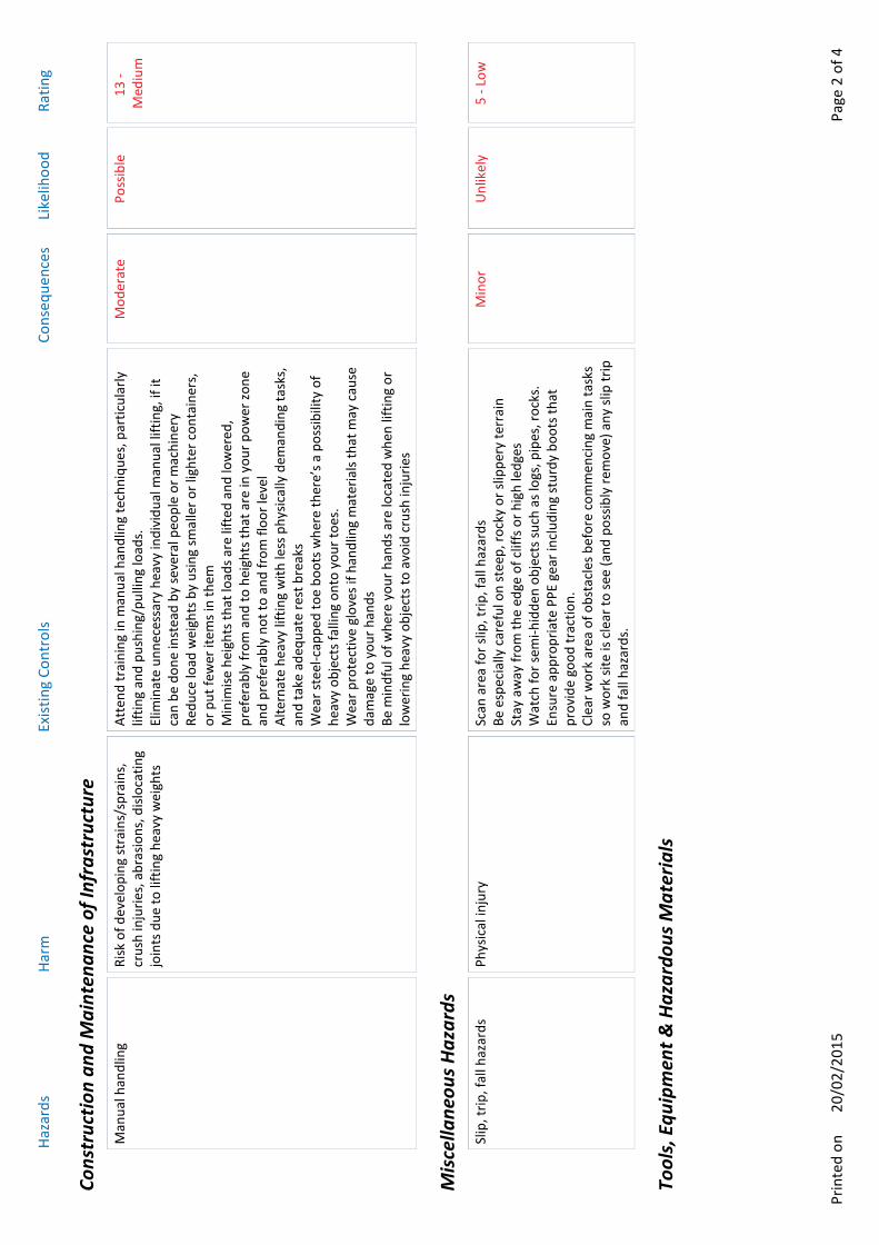
Haza
rds
Harm
Exist
ing
Cont
rols
Cons
eque
nces
Like
lihoo
dRa
ting
Cons
truc
tion
and
Mai
nten
ance
of I
nfra
stru
ctur
eM
anua
l han
dlin
gRi
sk o
f dev
elop
ing
stra
ins/
spra
ins,
cr
ush
inju
ries,
abra
sions
, disl
ocat
ing
join
ts d
ue to
lifti
ng h
eavy
wei
ghts
Atte
nd tr
aini
ng in
man
ual h
andl
ing
tech
niqu
es, p
artic
ular
ly
liftin
g an
d pu
shin
g/pu
lling
load
s.El
imin
ate
unne
cess
ary
heav
y in
divi
dual
man
ual l
iftin
g, if
it
can
be d
one
inst
ead
by se
vera
l peo
ple
or m
achi
nery
Redu
ce lo
ad w
eigh
ts b
y us
ing
smal
ler o
r lig
hter
con
tain
ers,
or p
ut fe
wer
item
s in
them
Min
imise
hei
ghts
that
load
s are
lift
ed a
nd lo
wer
ed,
pref
erab
ly fr
om a
nd to
hei
ghts
that
are
in y
our p
ower
zone
an
d pr
efer
ably
not
to a
nd fr
om fl
oor l
evel
Alte
rnat
e he
avy
liftin
g w
ith le
ss p
hysic
ally
dem
andi
ng ta
sks,
an
d ta
ke a
dequ
ate
rest
bre
aks
Wea
r ste
el-c
appe
d to
e bo
ots w
here
ther
e’s a
pos
sibili
ty o
f he
avy
obje
cts f
allin
g on
to y
our t
oes.
Wea
r pro
tect
ive
glov
es if
han
dlin
g m
ater
ials
that
may
cau
se
dam
age
to y
our h
ands
Be m
indf
ul o
f whe
re y
our h
ands
are
loca
ted
whe
n lif
ting
or
low
erin
g he
avy
obje
cts t
o av
oid
crus
h in
jurie
s
Mod
erat
ePo
ssib
le13
- M
ediu
m
Mis
cella
neou
s Haz
ards
Slip
, trip
, fal
l haz
ards
Phys
ical
inju
rySc
an a
rea
for s
lip, t
rip, f
all h
azar
dsBe
esp
ecia
lly c
aref
ul o
n st
eep,
rock
y or
slip
pery
terr
ain
Stay
aw
ay fr
om th
e ed
ge o
f clif
fs o
r hig
h le
dges
Wat
ch fo
r sem
i-hid
den
obje
cts s
uch
as lo
gs, p
ipes
, roc
ks.
Ensu
re a
ppro
pria
te P
PE g
ear i
nclu
ding
stur
dy b
oots
that
pr
ovid
e go
od tr
actio
n.Cl
ear w
ork
area
of o
bsta
cles
bef
ore
com
men
cing
mai
n ta
sks
so w
ork
site
is cl
ear t
o se
e (a
nd p
ossib
ly re
mov
e) a
ny sl
ip tr
ip
and
fall
haza
rds.
Min
orU
nlik
ely
5 - L
ow
Tool
s, E
quip
men
t & H
azar
dous
Mat
eria
ls
Page
2 o
f 420
/02/
2015
Prin
ted
on

Haza
rds
Harm
Exist
ing
Cont
rols
Cons
eque
nces
Like
lihoo
dRa
ting
Hand
tool
s (e.
g. h
amm
ers,
sle
dgeh
amm
ers,
pile
dr
iver
s, w
ood
saw
s,
hack
saw
s)
Phys
ical
inju
ry su
ch a
s cru
shin
g, c
uts
or a
bras
ions
Expe
rienc
ed st
aff n
eed
to c
oach
new
recr
uits
who
are
not
fa
mili
ar w
ith v
ario
us h
and
tool
s on
the
prop
er w
ay to
use
th
em.
Whe
n pi
le d
rivin
g lo
ng p
ipes
, use
a st
epla
dder
if c
onsid
ered
ne
cess
ary.
Sec
ure
it to
nea
rby
fixtu
res w
ith st
rong
taut
rope
sU
se 2
or 3
peo
ple
to li
ft p
ile d
river
s ont
o lo
ng p
ipes
Don’
t lift
pile
driv
ers s
o hi
gh w
hen
driv
ing
that
they
can
fall
off t
he p
ipe
or p
ost b
eing
driv
en.
Keep
han
ds w
ell a
way
from
impa
ct p
oint
of s
ledg
eham
mer
if
you
are
assis
ting
with
ope
ratio
ns
Mod
erat
eRa
re6
- Low
Pow
er to
ols (
e.g.
ele
ctric
sa
ws,
jack
ham
mer
s,
rota
ry a
nd h
amm
er d
rills,
gr
inde
rs e
tc)
Elec
tric
shoc
k or
in w
orst
cas
e sc
enar
io d
eath
from
ele
ctro
cutio
n.
Risk
of s
ever
e cu
ts a
nd a
bras
ions
.
Use
dou
ble-
insu
late
d po
wer
tool
sDo
n’t o
pera
te p
ower
tool
s whe
n st
andi
ng in
or n
ext t
o w
ater
.Ex
perie
nced
staf
f nee
d to
trai
n ne
w re
crui
ts in
ope
ratio
n of
to
ols i
f the
y ar
e no
t fam
iliar
with
how
to u
se th
em sa
fely
Use
a sa
fety
face
shie
ld w
hen
usin
g a
brus
h cu
tter
to g
uard
ag
ains
t stic
ks e
tc b
eing
thro
wn
up a
nd in
jurin
g yo
ur fa
ce.
Use
wha
teve
r saf
ety
equi
pmen
t is a
ppro
pria
te fo
r the
pow
er
tool
bei
ng u
sed
(e.g
. saf
ety
gogg
les o
r gla
sses
, ear
muf
fs,
glov
es)
Use
ear
th le
akag
e un
it w
ith g
ener
ator
s in
the
field
Mod
erat
eU
nlik
ely
9 -
Med
ium
Vehi
cles
& D
rivin
gCh
angi
ng a
flat
tyre
Refe
r to
Safe
Wor
k Pr
actic
e ST
HSW
P017
Mod
erat
eRa
re6
- Low
Wal
king In
bus
hlan
d - S
nake
sIll
ness
or d
eath
from
snak
e bi
teAl
way
s sca
n fo
r sna
kes
Mak
e no
ise w
hen
appr
oach
ing
wor
k ar
eaBe
aw
are
of p
oten
tial s
nake
refu
ge (e
.g. f
alle
n tim
ber,
tyre
s,
shee
t tin
, roc
ks)
Clea
r gra
ss &
veg
etat
ion
arou
nd w
ork
area
whe
re p
ossib
lePP
E - l
ong
pant
s and
stur
dy b
oots
Don’
t con
fron
t sna
kes,
allo
w th
em to
mov
e ou
t of t
he w
ay
befo
re c
ontin
uing
Staf
f to
have
cur
rent
firs
t aid
qua
lific
atio
ns &
refr
esh
on
snak
e bi
te p
roce
dure
sO
pen
inst
rum
ent h
ut d
oors
car
eful
ly b
efor
e en
terin
g
Min
orRa
re3
- Low
Page
3 o
f 420
/02/
2015
Prin
ted
on

Haza
rds
Harm
Exist
ing
Cont
rols
Cons
eque
nces
Like
lihoo
dRa
ting
Slip
ping
, trip
ping
, or
falli
ng fr
om h
eigh
tPo
ssib
le p
hysic
al in
jury
such
as
stra
ins,
spra
ins o
r bre
aks
Be e
spec
ially
car
eful
on
stee
p ro
cky
or sl
ippe
ry sl
opes
, w
here
any
boo
ts c
an b
e re
lativ
ely
inef
fect
ual,
part
icul
arly
if
wet
or c
over
ed w
ith g
rass
.St
ay a
way
from
, or e
xerc
ise e
xtre
me
caut
ion
near
the
edge
of
clif
fs o
r hig
h le
dges
.U
se tr
acks
that
hav
e pr
evio
usly
bee
n sa
fely
neg
otia
ted
On
very
stee
p st
ream
ban
ks, i
nsta
ll gu
ide
rails
or u
se a
stro
ng
rope
secu
red
to a
robu
st m
ount
ing
poin
t, to
hel
p ke
ep y
our
foot
ing
Inst
all p
ipe
acce
ss la
dder
s to
read
gau
ge b
oard
s in
deep
w
ater
nea
r ste
ep b
anks
Wea
r wor
k bo
ots o
r div
e bo
ots w
ith g
ood
trea
ds
Min
orU
nlik
ely
5 - L
ow
Wat
er -
In (e
.g. w
adin
g ga
ugin
gs, w
ater
sam
plin
g, st
atio
n m
aint
enan
ce)
Slip
ping
or t
rippi
ngPh
ysic
al in
jury
cau
sed
by lo
sing
foot
hold
Be e
spec
ially
car
eful
in st
ream
s with
mos
s-co
vere
d ro
cks
Wea
r div
e bo
ots o
r wad
ers w
ith fe
lted
sole
s tha
t grip
bet
ter
on ro
cks
Min
orU
nlik
ely
5 - L
ow
Wea
ther
Eve
nts
Heat
and
sun
expo
sure
Refe
r to
Safe
Wor
k Pr
actic
e ST
HSW
P008
Mod
erat
ePo
ssib
le13
- M
ediu
m
Addi
tiona
l Con
trol
s
Page
4 o
f 420
/02/
2015
Prin
ted
on

Appendix C
As Built Channel Drawings


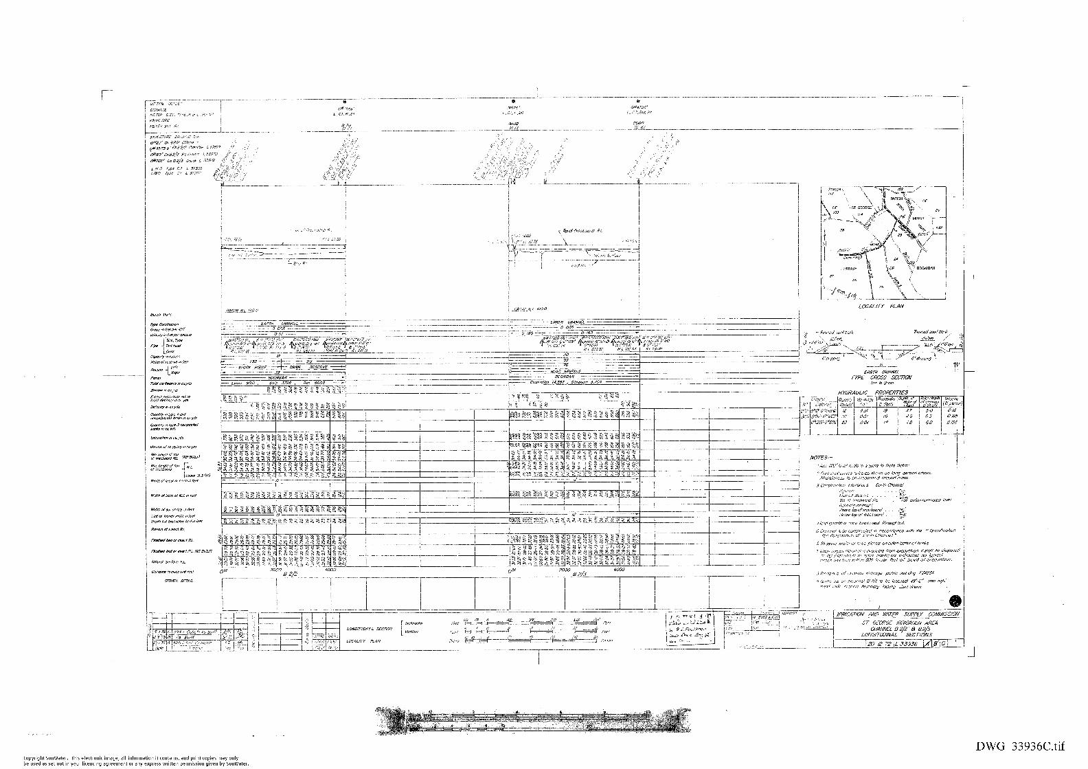

Appendix D
Rainfall Data
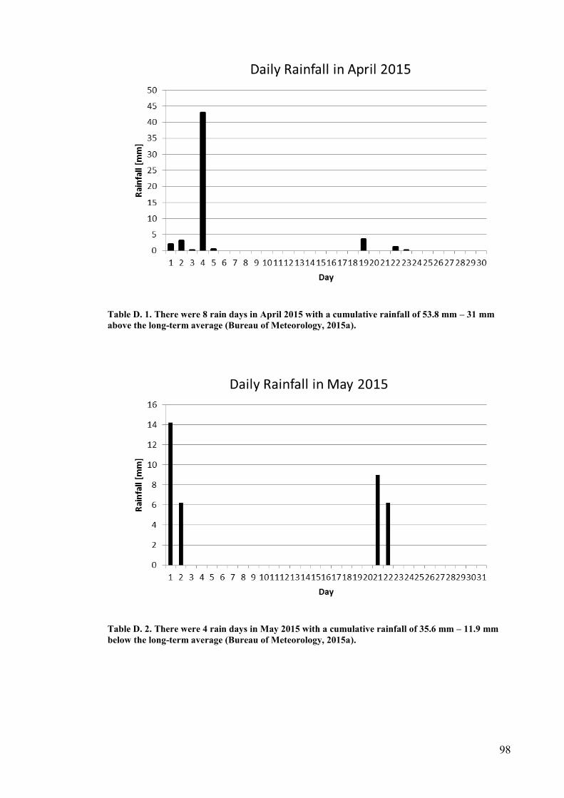
98
Table D. 1. There were 8 rain days in April 2015 with a cumulative rainfall of 53.8 mm – 31 mm above the long-term average (Bureau of Meteorology, 2015a).
Table D. 2. There were 4 rain days in May 2015 with a cumulative rainfall of 35.6 mm – 11.9 mm below the long-term average (Bureau of Meteorology, 2015a).

99
Table D. 3. The cumulative evapotranspiration during April 2015 was 199.3 mm (Bureau of Meteorology, 2015b).
Table D. 4. The cumulative evapotranspiration during May 2015 was 88.1 mm (Bureau of Meteorology, 2015b).

Appendix E
Summary Data for Seepage Losses
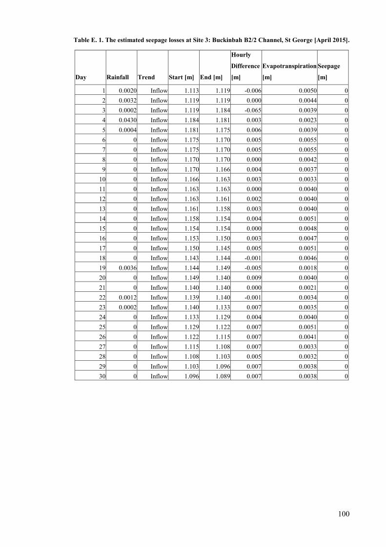
100
Table E. 1. The estimated seepage losses at Site 3: Buckinbah B2/2 Channel, St George [April 2015].
Day Rainfall Trend Start [m] End [m]
Hourly
Difference
[m]
Evapotranspiration
[m]
Seepage
[m]
1 0.0020 Inflow 1.113 1.119 -0.006 0.0050 0
2 0.0032 Inflow 1.119 1.119 0.000 0.0044 0
3 0.0002 Inflow 1.119 1.184 -0.065 0.0039 0
4 0.0430 Inflow 1.184 1.181 0.003 0.0023 0
5 0.0004 Inflow 1.181 1.175 0.006 0.0039 0
6 0 Inflow 1.175 1.170 0.005 0.0055 0
7 0 Inflow 1.175 1.170 0.005 0.0055 0
8 0 Inflow 1.170 1.170 0.000 0.0042 0
9 0 Inflow 1.170 1.166 0.004 0.0037 0
10 0 Inflow 1.166 1.163 0.003 0.0033 0
11 0 Inflow 1.163 1.163 0.000 0.0040 0
12 0 Inflow 1.163 1.161 0.002 0.0040 0
13 0 Inflow 1.161 1.158 0.003 0.0040 0
14 0 Inflow 1.158 1.154 0.004 0.0051 0
15 0 Inflow 1.154 1.154 0.000 0.0048 0
16 0 Inflow 1.153 1.150 0.003 0.0047 0
17 0 Inflow 1.150 1.145 0.005 0.0051 0
18 0 Inflow 1.143 1.144 -0.001 0.0046 0
19 0.0036 Inflow 1.144 1.149 -0.005 0.0018 0
20 0 Inflow 1.149 1.140 0.009 0.0040 0
21 0 Inflow 1.140 1.140 0.000 0.0021 0
22 0.0012 Inflow 1.139 1.140 -0.001 0.0034 0
23 0.0002 Inflow 1.140 1.133 0.007 0.0035 0
24 0 Inflow 1.133 1.129 0.004 0.0040 0
25 0 Inflow 1.129 1.122 0.007 0.0051 0
26 0 Inflow 1.122 1.115 0.007 0.0041 0
27 0 Inflow 1.115 1.108 0.007 0.0033 0
28 0 Inflow 1.108 1.103 0.005 0.0032 0
29 0 Inflow 1.103 1.096 0.007 0.0038 0
30 0 Inflow 1.096 1.089 0.007 0.0038 0

101
Table E. 2. The estimated seepage losses at Site 3: Buckinbah B2/2 Channel, St George [May 2015].
Day Rainfall Trend Start [m] End [m]
Hourly Difference [m]
Evapotranspiration [m]
Seepage [m]
1 0.1420 Inflow 1.089 1.091 -0.002 0.0017 0
2 0.0620 Inflow 1.091 1.088 0.003 0.0021 0
3 0 Inflow 1.088 1.084 0.004 0.0035 0
4 0 Inflow 1.084 1.081 0.003 0.0034 0
5 0 Inflow 1.081 1.079 0.002 0.0034 0
6 0 Inflow 1.081 1.081 0.000 0.0037 0
7 0 Inflow 1.081 1.081 0.000 0.0033 0
8 0 Inflow 1.081 1.076 0.005 0.0030 0
9 0 Inflow 1.076 1.073 0.003 0.0025 0
10 0 Inflow 1.076 1.073 0.003 0.0030 0
11 0 Inflow 1.073 1.073 0.000 0.0037 0
12 0 Inflow 1.073 1.076 -0.003 0.0026 0
13 0 Inflow 1.076 1.072 0.004 0.0034 0
14 0 Inflow 1.072 1.066 0.006 0.0035 0
15 0 Inflow 1.066 1.066 0.000 0.0026 0
16 0 Inflow 1.066 1.064 0.002 0.0033 0
17 0 Inflow 1.064 1.064 0.000 0.0028 0
18 0 Inflow 1.064 1.064 0.000 0.0032 0
19 0 Falling 1.064 1.055 0.009 0.0028 0.006
20 0 Falling 1.055 1.041 0.014 0.0034 0.011
21 0.0090 Falling 1.041 1.035 0.006 0.0012 0.005
22 0.0062 Falling 1.034 1.019 0.015 0.0020 0.013
23 0 Falling 1.019 1.007 0.012 0.0026 0.009
24 0 Falling 1.007 0.998 0.009 0.0026 0.006
25 0 Falling 0.998 0.987 0.011 0.0028 0.008
26 0 Falling 0.987 0.977 0.010 0.0023 0.008
27 0 Falling 0.977 0.971 0.006 0.0023 0.004
28 0 Falling 0.971 0.961 0.010 0.0023 0.008
29 0 Falling 0.959 0.953 0.006 0.0034 0
30 0 Falling 0.953 0.949 0.004 0.0030 0
31 0 Falling 0.949 0.942 0.007 0.0027 0

102
Table E. 3. The estimated seepage losses at Site 2: Buckinbah B2 Channel, St George [April 2015].
Day Rainfall Trend Start [m] End [m]
Hourly Difference [m]
Evapotranspiration [m]
Seepage [m]
1 0.0020 Inflow 0.342 0.309 0.033 0.0050 0
2 0.0032 Inflow 0.309 0.376 -0.067 0.0044 0
3 0.0002 Inflow 0.376 0.354 0.022 0.0039 0
4 0.0430 Inflow 0.354 0.278 0.076 0.0023 0
5 0.0004 Inflow 0.278 0.327 -0.049 0.0039 0
6 0 Falling 0.327 0.348 -0.021 0.0055 0
7 0 Falling 0.348 0.302 0.046 0.0055 0
8 0 Falling 0.302 0.236 0.066 0.0042 0
9 0 Falling 0.236 0.230 0.006 0.0037 0
10 0 Falling 0.23 0.243 -0.013 0.0033 0
11 0 Falling 0.243 0.235 0.008 0.0040 0
12 0 Falling 0.235 0.228 0.007 0.0040 0
13 Falling 0.228 0.219 0.009 0.0040 0
14 0 Falling 0.219 0.210 0.009 0.0051 0
15 0 Falling 0.21 0.197 0.013 0.0048 0.0082
16 0 Falling 0.197 0.191 0.006 0.0047 0
17 0 Falling 0.191 0.175 0.016 0.0051 0.0109
18 0 Falling 0.175 0.172 0.003 0.0046 0
19 0.0036 Inflow 0.172 0.172 0.000 0.0018 0
20 0 Inflow 0.172 0.157 0.015 0.0040 0.011
21 0 Inflow 0.157 0.152 0.005 0.0021 0
22 0.0012 Inflow 0.152 0.146 0.006 0.0034 0
23 0.0002 Inflow 0.146 0.143 0.003 0.0035 -0.0005
24 0 Falling 0.143 0.137 0.006 0.0040 0
25 0 Falling 0.137 0.127 0.010 0.0051 0
26 0 Falling 0.127 0.119 0.008 0.0041 0
27 0 Falling 0.119 0.111 0.008 0.0033 0
28 0 Falling 0.111 0.107 0.004 0.0032 0
29 0 Falling 0.107 0.095 0.012 0.0038 0.0082
30 0 Falling 0.095 0.092 0.003 0.0038 0
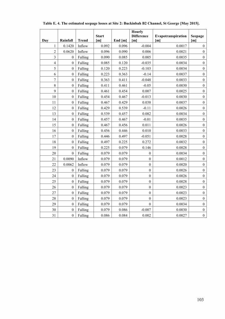
103
Table E. 4. The estimated seepage losses at Site 2: Buckinbah B2 Channel, St George [May 2015].
Day Rainfall Trend Start [m] End [m]
Hourly Difference [m]
Evapotranspiration [m]
Seepage [m]
1 0.1420 Inflow 0.092 0.096 -0.004 0.0017 0
2 0.0620 Inflow 0.096 0.090 0.006 0.0021 0
3 0 Falling 0.090 0.085 0.005 0.0035 0
4 0 Falling 0.085 0.120 -0.035 0.0034 0
5 0 Falling 0.120 0.223 -0.103 0.0034 0
6 0 Falling 0.223 0.363 -0.14 0.0037 0
7 0 Falling 0.363 0.411 -0.048 0.0033 0
8 0 Falling 0.411 0.461 -0.05 0.0030 0
9 0 Falling 0.461 0.454 0.007 0.0025 0
10 0 Falling 0.454 0.467 -0.013 0.0030 0
11 0 Falling 0.467 0.429 0.038 0.0037 0
12 0 Falling 0.429 0.539 -0.11 0.0026 0
13 0 Falling 0.539 0.457 0.082 0.0034 0
14 0 Falling 0.457 0.467 -0.01 0.0035 0
15 0 Falling 0.467 0.456 0.011 0.0026 0
16 0 Falling 0.456 0.446 0.010 0.0033 0
17 0 Falling 0.446 0.497 -0.051 0.0028 0
18 0 Falling 0.497 0.225 0.272 0.0032 0
19 0 Falling 0.225 0.079 0.146 0.0028 0
20 0 Falling 0.079 0.079 0 0.0034 0
21 0.0090 Inflow 0.079 0.079 0 0.0012 0
22 0.0062 Inflow 0.079 0.079 0 0.0020 0
23 0 Falling 0.079 0.079 0 0.0026 0
24 0 Falling 0.079 0.079 0 0.0026 0
25 0 Falling 0.079 0.079 0 0.0028 0
26 0 Falling 0.079 0.079 0 0.0023 0
27 0 Falling 0.079 0.079 0 0.0023 0
28 0 Falling 0.079 0.079 0 0.0023 0
29 0 Falling 0.079 0.079 0 0.0034 0
30 0 Falling 0.079 0.086 -0.007 0.0030 0
31 0 Falling 0.086 0.084 0.002 0.0027 0
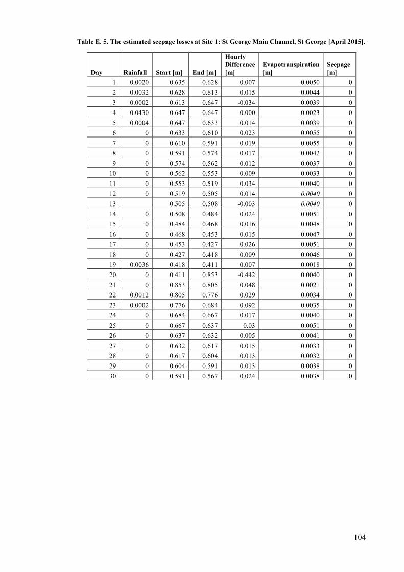
104
Table E. 5. The estimated seepage losses at Site 1: St George Main Channel, St George [April 2015].
Day Rainfall Start [m] End [m]
Hourly Difference [m]
Evapotranspiration [m]
Seepage [m]
1 0.0020 0.635 0.628 0.007 0.0050 0
2 0.0032 0.628 0.613 0.015 0.0044 0
3 0.0002 0.613 0.647 -0.034 0.0039 0
4 0.0430 0.647 0.647 0.000 0.0023 0
5 0.0004 0.647 0.633 0.014 0.0039 0
6 0 0.633 0.610 0.023 0.0055 0
7 0 0.610 0.591 0.019 0.0055 0
8 0 0.591 0.574 0.017 0.0042 0
9 0 0.574 0.562 0.012 0.0037 0
10 0 0.562 0.553 0.009 0.0033 0
11 0 0.553 0.519 0.034 0.0040 0
12 0 0.519 0.505 0.014 0.0040 0
13 0.505 0.508 -0.003 0.0040 0
14 0 0.508 0.484 0.024 0.0051 0
15 0 0.484 0.468 0.016 0.0048 0
16 0 0.468 0.453 0.015 0.0047 0
17 0 0.453 0.427 0.026 0.0051 0
18 0 0.427 0.418 0.009 0.0046 0
19 0.0036 0.418 0.411 0.007 0.0018 0
20 0 0.411 0.853 -0.442 0.0040 0
21 0 0.853 0.805 0.048 0.0021 0
22 0.0012 0.805 0.776 0.029 0.0034 0
23 0.0002 0.776 0.684 0.092 0.0035 0
24 0 0.684 0.667 0.017 0.0040 0
25 0 0.667 0.637 0.03 0.0051 0
26 0 0.637 0.632 0.005 0.0041 0
27 0 0.632 0.617 0.015 0.0033 0
28 0 0.617 0.604 0.013 0.0032 0
29 0 0.604 0.591 0.013 0.0038 0
30 0 0.591 0.567 0.024 0.0038 0

105
Table E. 6. The estimated seepage losses at Site 1: St George Main Channel, St George [May 2015].
Day Rainfall Start [m] End [m]
Hourly Difference [m]
Evapotranspiration [m]
Seepage [m]
1 0.0142 0.567 0.576 -0.009 0.0017 0
2 0.0062 0.576 0.714 -0.138 0.0021 0
3 0 0.714 0.681 0.033 0.0035 0
4 0 0.681 0.659 0.022 0.0034 0
5 0 0.659 0.641 0.018 0.0034 0
6 0 0.641 0.627 0.014 0.0037 0
7 0 0.627 0.627 0.000 0.0033 0
8 0 0.627 0.613 0.014 0.0030 0
9 0 0.613 0.593 0.020 0.0025 0
10 0 0.593 0.639 -0.046 0.0030 0
11 0 0.639 0.694 -0.055 0.0037 0
12 0 0.694 0.727 -0.033 0.0026 0
13 0 0.727 0.727 0.000 0.0034 0
14 0 0.727 0.726 0.001 0.0035 0
15 0 0.726 0.708 0.018 0.0026 0
16 0 0.708 0.708 0.000 0.0033 0
17 0 0.708 0.695 0.013 0.0028 0
18 0 0.695 0.698 -0.003 0.0032 0
19 0 0.698 0.711 -0.013 0.0028 0
20 0 0.711 0.730 -0.019 0.0034 0
21 0.009 0.730 0.730 0.000 0.0012 0
22 0.0062 0.730 0.730 0.000 0.0020 0
23 0 0.730 0.724 0.006 0.0026 0
24 0 0.724 0.728 -0.004 0.0026 0
25 0 0.728 0.698 0.030 0.0028 0
26 0 0.698 0.670 0.028 0.0023 0
27 0 0.670 0.665 0.005 0.0023 0
28 0 0.665 0.655 0.010 0.0023 0
29 0 0.655 0.641 0.014 0.0034 0
30 0 0.641 0.632 0.009 0.0030 0
31 0 0.632 0.631 0.001 0.0027 0
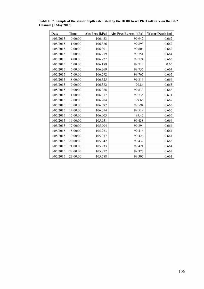
106
Table E. 7. Sample of the sensor depth calculated by the HOBOware PRO software on the B2/2 Channel [1 May 2015].
Date Time Abs Pres [kPa] Abs Pres Barom [kPa] Water Depth [m]
1/05/2015 0:00:00 106.433 99.942 0.662
1/05/2015 1:00:00 106.386 99.893 0.662
1/05/2015 2:00:00 106.301 99.806 0.662
1/05/2015 3:00:00 106.259 99.751 0.664
1/05/2015 4:00:00 106.227 99.724 0.663
1/05/2015 5:00:00 106.189 99.713 0.66
1/05/2015 6:00:00 106.269 99.756 0.664
1/05/2015 7:00:00 106.292 99.767 0.665
1/05/2015 8:00:00 106.325 99.816 0.664
1/05/2015 9:00:00 106.382 99.86 0.665
1/05/2015 10:00:00 106.368 99.833 0.666
1/05/2015 11:00:00 106.317 99.735 0.671
1/05/2015 12:00:00 106.204 99.66 0.667
1/05/2015 13:00:00 106.092 99.594 0.663
1/05/2015 14:00:00 106.054 99.519 0.666
1/05/2015 15:00:00 106.003 99.47 0.666
1/05/2015 16:00:00 105.951 99.438 0.664
1/05/2015 17:00:00 105.904 99.394 0.664
1/05/2015 18:00:00 105.923 99.416 0.664
1/05/2015 19:00:00 105.937 99.426 0.664
1/05/2015 20:00:00 105.942 99.437 0.663
1/05/2015 21:00:00 105.933 99.421 0.664
1/05/2015 22:00:00 105.872 99.377 0.662
1/05/2015 23:00:00 105.788 99.307 0.661
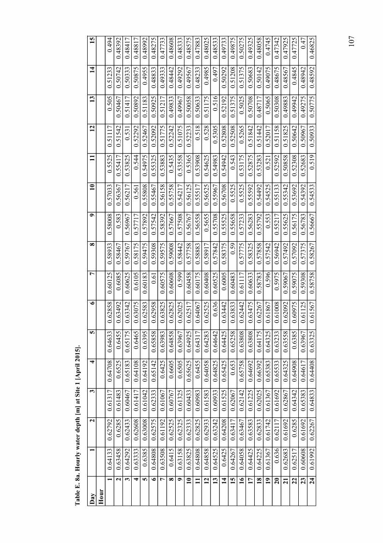
107
Tabl
e E
. 8a.
Hou
rly
wat
er d
epth
[m] a
t Site
1 [A
pril
2015
].
Day
12
34
56
78
910
1112
1314
15Hour
10.64133
0.62792
0.61317
0.64708
0.64633
0.62858
0.60125
0.58933
0.58008
0.57033
0.5525
0.51117
0.505
0.51233
0.494
20.63458
0.6285
0.61483
0.6525
0.6455
0.63492
0.6085
0.58467
0.583
0.56367
0.55417
0.51542
0.50467
0.50742
0.48392
30.64292
0.62433
0.60467
0.65183
0.65175
0.63342
0.60625
0.59767
0.56967
0.56217
0.53825
0.531
0.51417
0.50333
0.48417
40.63333
0.62608
0.61417
0.64108
0.6465
0.63075
0.6105
0.58175
0.57717
0.561
0.544
0.52292
0.50892
0.50875
0.48817
50.6385
0.63008
0.61042
0.64192
0.6395
0.62583
0.60183
0.59475
0.57892
0.55808
0.54975
0.52467
0.51183
0.4955
0.48992
60.64808
0.62575
0.62333
0.65142
0.65858
0.62958
0.61
0.59308
0.57542
0.55467
0.55325
0.52092
0.50925
0.48833
0.48275
70.63508
0.61192
0.61067
0.6425
0.63983
0.63825
0.60575
0.59575
0.58392
0.56158
0.53883
0.51775
0.51217
0.49333
0.47733
80.6415
0.62525
0.60767
0.6605
0.64858
0.62825
0.60608
0.59008
0.57667
0.55758
0.5435
0.52242
0.49833
0.48442
0.48608
90.63158
0.62325
0.61325
0.6505
0.63967
0.62025
0.599
0.58442
0.57508
0.54217
0.53558
0.51075
0.49967
0.49292
0.48333
100.63825
0.62333
0.60433
0.65625
0.64925
0.62517
0.60458
0.57758
0.56767
0.56125
0.5365
0.52233
0.50058
0.49567
0.48575
110.64808
0.62825
0.60983
0.6455
0.64317
0.64067
0.60175
0.58883
0.56558
0.55517
0.53908
0.518
0.50633
0.48233
0.47883
120.64858
0.62933
0.61583
0.64058
0.64283
0.62525
0.60408
0.58917
0.5655
0.56525
0.54625
0.528
0.51175
0.4985
0.48025
130.64525
0.63242
0.60933
0.64825
0.64642
0.636
0.60525
0.57842
0.55708
0.55967
0.54983
0.5305
0.516
0.497
0.48533
140.6425
0.64208
0.61525
0.65425
0.64425
0.63442
0.6005
0.58375
0.55525
0.56708
0.54942
0.52808
0.52192
0.50292
0.49733
150.64267
0.63417
0.62067
0.653
0.65258
0.63833
0.60483
0.59
0.55658
0.5525
0.543
0.52508
0.51375
0.51208
0.49875
160.64058
0.63467
0.62142
0.65758
0.63808
0.62442
0.61117
0.57775
0.57233
0.5525
0.53175
0.5265
0.5025
0.51375
0.50275
170.64425
0.63583
0.61225
0.64692
0.63808
0.63475
0.60633
0.58325
0.56283
0.55592
0.52875
0.51842
0.50708
0.50683
0.49325
180.64225
0.62833
0.62025
0.66392
0.64175
0.62267
0.58783
0.57858
0.55792
0.54492
0.53283
0.51442
0.48717
0.50142
0.48058
190.61367
0.61742
0.61367
0.65383
0.64325
0.61867
0.596
0.57542
0.553
0.54525
0.521
0.52017
0.5065
0.49075
0.4745
200.636
0.62117
0.61692
0.65533
0.63233
0.61008
0.5975
0.56942
0.55217
0.55133
0.52592
0.51158
0.50308
0.48675
0.47342
210.62683
0.61692
0.62867
0.64325
0.63558
0.62092
0.59067
0.57492
0.55625
0.55342
0.50858
0.51825
0.49883
0.48567
0.47925
220.62517
0.6285
0.64342
0.64908
0.6385
0.60975
0.59075
0.57092
0.56175
0.53692
0.52308
0.50642
0.49942
0.4845
0.47725
230.60608
0.61692
0.65383
0.64617
0.63967
0.61125
0.59308
0.57375
0.56783
0.54392
0.52683
0.50967
0.49275
0.48942
0.47
240.61992
0.62267
0.64833
0.64408
0.63325
0.61567
0.58758
0.58267
0.56667
0.54533
0.519
0.50933
0.50775
0.48592
0.46825

108
Tabl
e E
. 8b.
Hou
rly
wat
er d
epth
[m] a
t Site
1 [A
pril
2015
].
Day
1617
1819
2021
2223
2425
2627
2829
30Hour
10.46333
0.45625
0.42658
0.4105
0.41142
0.82308
0.8035
0.77592
0.68642
0.66442
0.64283
0.637
0.61658
0.60375
0.59067
20.4665
0.45533
0.4205
0.4175
0.40183
0.83775
0.80517
0.76717
0.68375
0.67275
0.63617
0.6265
0.62925
0.6055
0.58225
30.47183
0.453
0.42625
0.42142
0.41133
0.83075
0.80942
0.774
0.68142
0.66842
0.63242
0.63108
0.61967
0.5985
0.59242
40.468
0.46183
0.43658
0.41358
0.41275
0.81708
0.80742
0.76408
0.67383
0.66725
0.63017
0.62992
0.61675
0.60858
0.5845
50.45675
0.45725
0.4285
0.43008
0.40958
0.82575
0.81458
0.76458
0.66975
0.67558
0.63975
0.63458
0.61208
0.60075
0.57817
60.45967
0.45383
0.43633
0.41658
0.40842
0.83125
0.81117
0.7655
0.66658
0.66433
0.63492
0.62767
0.62342
0.5985
0.58392
70.47158
0.4585
0.42483
0.42325
0.4035
0.82175
0.81492
0.7545
0.65883
0.66292
0.63817
0.6225
0.61367
0.60458
0.58542
80.45958
0.45342
0.42833
0.423
0.40758
0.82433
0.81233
0.75833
0.66842
0.66417
0.63933
0.63875
0.60042
0.60008
0.57825
90.45192
0.44717
0.43508
0.42508
0.40208
0.82383
0.8115
0.74425
0.66383
0.66908
0.63167
0.6285
0.61125
0.58233
0.58208
100.46758
0.45675
0.43142
0.4145
0.403
0.79717
0.79833
0.74017
0.67342
0.65608
0.63208
0.62567
0.61017
0.58708
0.57408
110.4615
0.459
0.42875
0.41225
0.40017
0.80258
0.80325
0.72617
0.68025
0.66067
0.63092
0.62367
0.60325
0.59375
0.57492
120.46667
0.45
0.42033
0.41742
0.40617
0.80392
0.81933
0.722
0.68833
0.66233
0.628
0.61725
0.60925
0.58275
0.58842
130.46733
0.45992
0.43375
0.42225
0.40533
0.79633
0.80108
0.71808
0.68758
0.65733
0.63025
0.62633
0.61233
0.59792
0.57042
140.47125
0.46325
0.42608
0.4135
0.44983
0.80317
0.7995
0.70867
0.68575
0.66708
0.63308
0.6245
0.61625
0.60583
0.58125
150.46917
0.45817
0.42225
0.41058
0.50433
0.7945
0.80083
0.71083
0.68625
0.66042
0.63042
0.62133
0.60892
0.57775
0.56325
160.478
0.46642
0.42508
0.4135
0.58383
0.78617
0.80717
0.70008
0.68392
0.65167
0.63183
0.62042
0.59533
0.58833
0.57125
170.45667
0.45142
0.42192
0.42358
0.66458
0.79942
0.80883
0.69942
0.6755
0.66408
0.6255
0.62592
0.606
0.584
0.58658
180.47942
0.45058
0.436
0.4135
0.71917
0.81017
0.81125
0.69567
0.664
0.6575
0.62583
0.61325
0.59908
0.58917
0.56783
190.46642
0.44533
0.40892
0.42075
0.76633
0.805
0.80117
0.68383
0.66408
0.64892
0.6455
0.61875
0.6005
0.59492
0.56325
200.45575
0.44417
0.4245
0.41533
0.79325
0.80617
0.81817
0.68042
0.66067
0.64842
0.63833
0.62542
0.61125
0.59033
0.57408
210.45775
0.42658
0.42367
0.41308
0.80725
0.80875
0.79908
0.67725
0.67342
0.64158
0.63983
0.61683
0.61475
0.57883
0.57267
220.45342
0.43642
0.422
0.403
0.82242
0.807
0.78492
0.68392
0.6665
0.64308
0.64075
0.62408
0.60258
0.57675
0.57675
230.46525
0.42817
0.41633
0.40042
0.82133
0.805
0.78625
0.6885
0.67025
0.63733
0.64275
0.612
0.59975
0.57217
0.56808
240.46292
0.43217
0.41717
0.41225
0.81208
0.80583
0.7815
0.68442
0.66617
0.64108
0.6315
0.61833
0.60375
0.58717
0.56142