Embed Size (px)
Citation preview
1
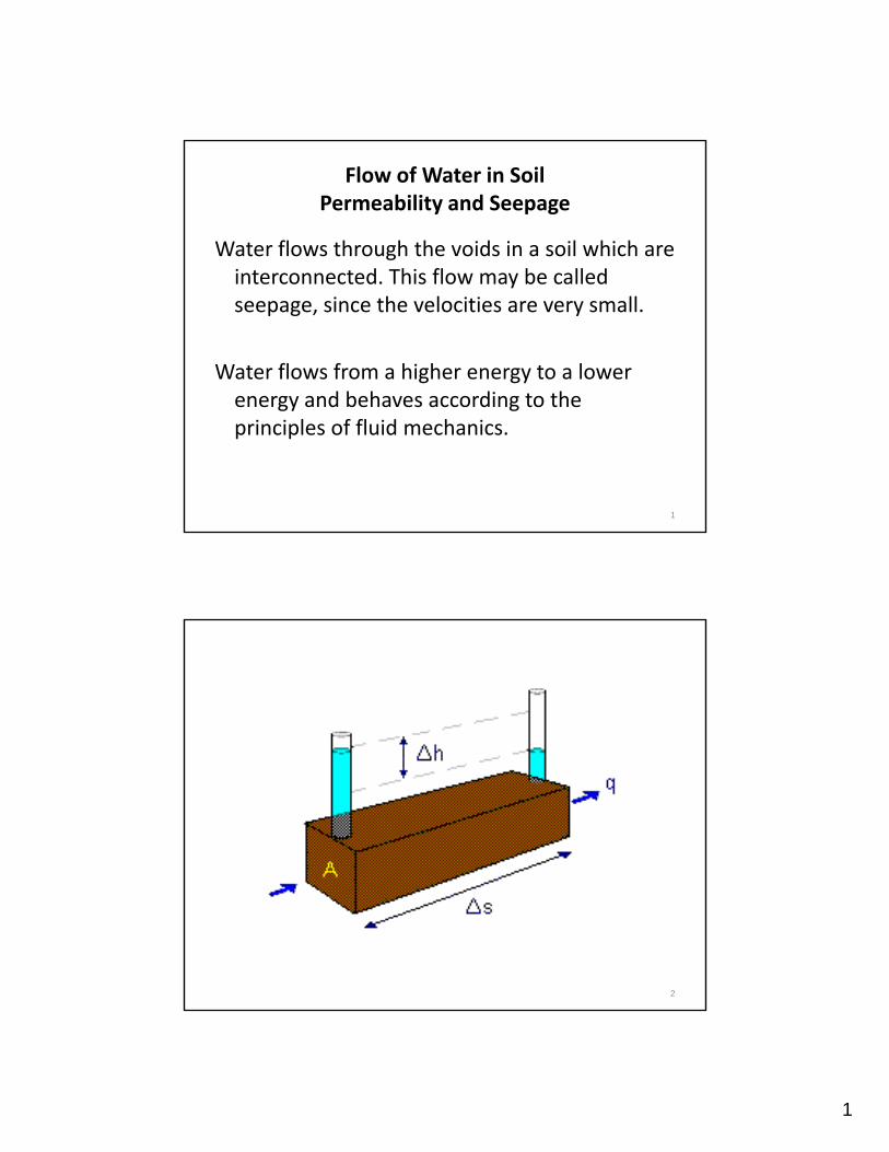
Flow of Water in Soil Permeability and Seepage
Water flows through the voids in a soil which are i t t d Thi fl b ll dinterconnected. This flow may be called seepage, since the velocities are very small.
Water flows from a higher energy to a lower energy and behaves according to theenergy and behaves according to the principles of fluid mechanics.
1
2
2
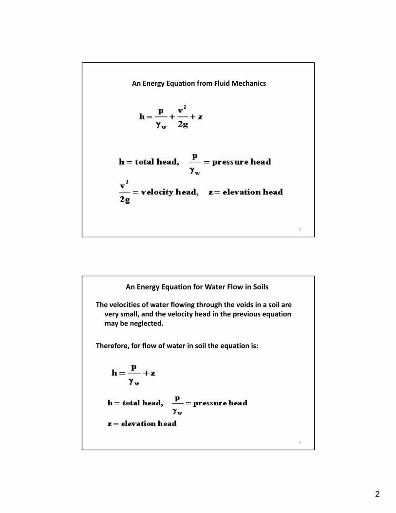
An Energy Equation from Fluid Mechanics
3
An Energy Equation for Water Flow in Soils
The velocities of water flowing through the voids in a soil are very small, and the velocity head in the previous equation may be neglected.
Therefore, for flow of water in soil the equation is:
4
3
Calculation of Heads
Basic Principles
• Total Head = Pressure Head + Elevation Head
• The pressure head is zero at a water surface.
• The head loss in the water is assumed to be zero.
• All head loss occurs in the soil.
5
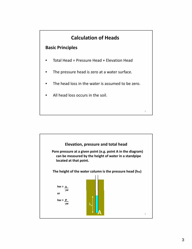
Elevation, pressure and total head
Pore pressure at a given point (e.g. point A in the diagram) can be measured by the height of water in a standpipe located at that point.p
The height of the water column is the pressure head (hw)
hw = uγw
6
γwor
hw = Pγw
4
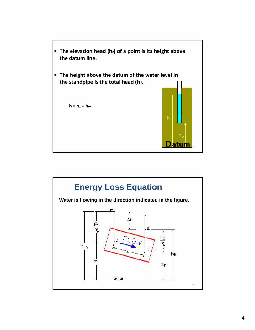
• The elevation head (hz) of a point is its height above the datum line.
• The height above the datum of the water level in gthe standpipe is the total head (h).
h = hz + hw
7
Water is flowing in the direction indicated in the figure.
Energy Loss Equation
8

5
Energy Loss Equation
9
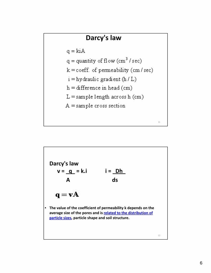
Darcy's law
• The rate of flow of water q (volume/time) through cross‐sectional area A is found to be proportional to hydraulic gradient i according to Darcy's law: to yd au c g ad e t acco d g to a cy s a :
10
6
Darcy's law
11
Darcy's lawv = q = k.i i = Dh
dA ds
• The value of the coefficient of permeability k depends on the
12
The value of the coefficient of permeability k depends on the average size of the pores and is related to the distribution of particle sizes, particle shape and soil structure.
7
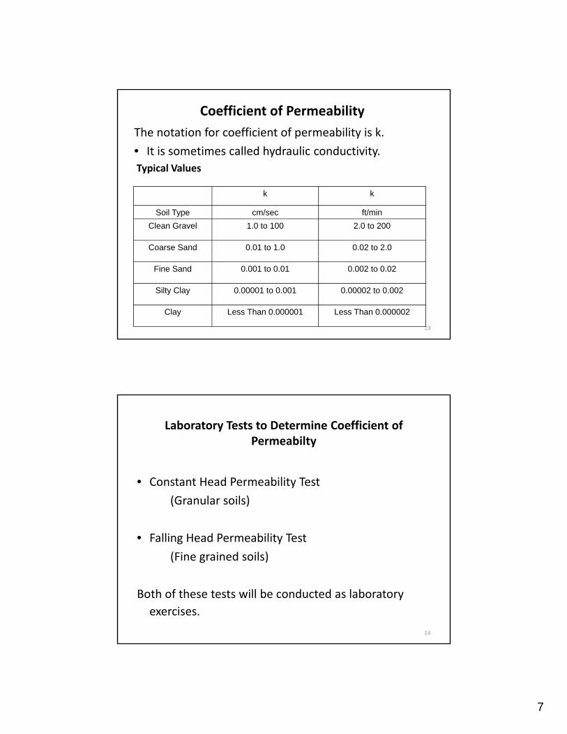
Coefficient of Permeability The notation for coefficient of permeability is k.
• It is sometimes called hydraulic conductivity.Typical Values yp
k k
Soil Type cm/sec ft/minClean Gravel 1.0 to 100 2.0 to 200
Coarse Sand 0.01 to 1.0 0.02 to 2.0
13
Fine Sand 0.001 to 0.01 0.002 to 0.02
Silty Clay 0.00001 to 0.001 0.00002 to 0.002
Clay Less Than 0.000001 Less Than 0.000002
Laboratory Tests to Determine Coefficient of Permeabilty
C d bili• Constant Head Permeability Test
(Granular soils)
• Falling Head Permeability Test
(Fine grained soils)( g )
Both of these tests will be conducted as laboratory exercises.
14
8
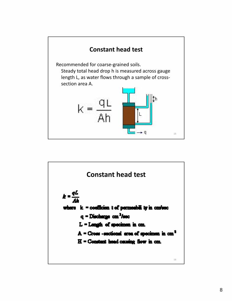
Constant head test
Recommended for coarse‐grained soils.Steady total head drop h is measured across gaugeSteady total head drop h is measured across gauge length L, as water flows through a sample of cross‐section area A.
15
Constant head test
16
9
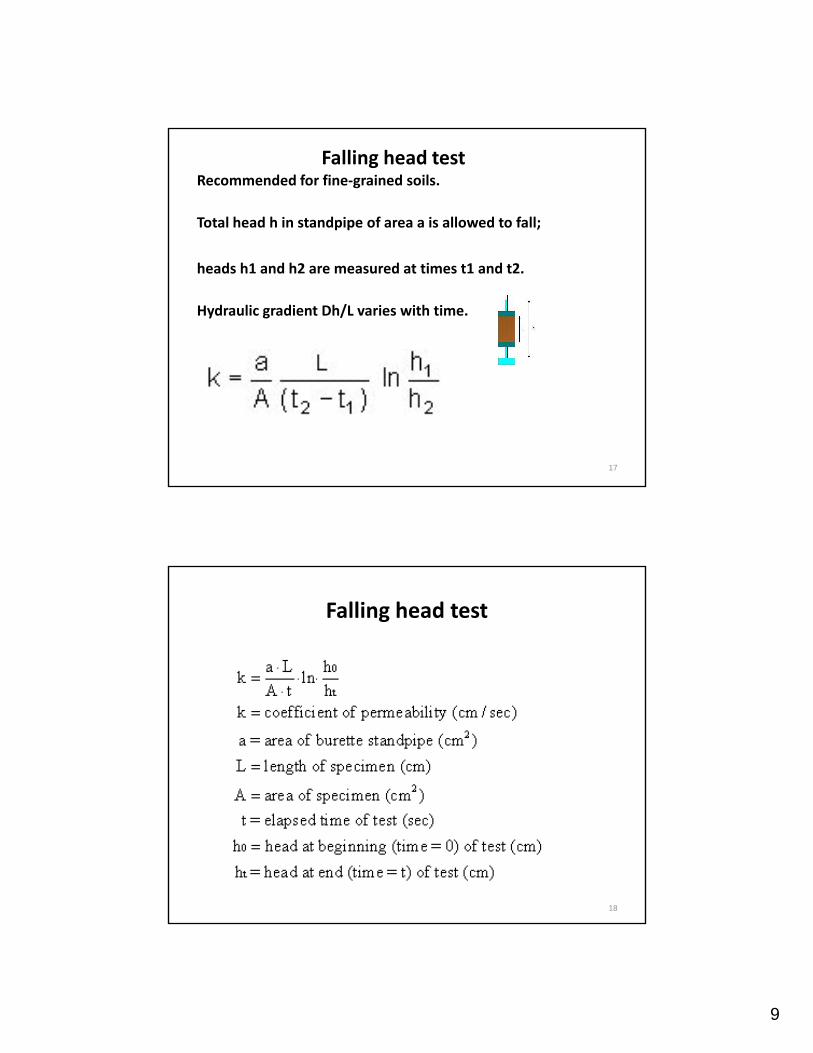
Falling head testRecommended for fine‐grained soils.
Total head h in standpipe of area a is allowed to fall;
heads h1 and h2 are measured at times t1 and t2.
Hydraulic gradient Dh/L varies with time.
17
Falling head test
18
10
Two‐Dimensional FlowSeepage and Flow Nets
• In the previous section the seepage problems discussed were all lab models consisting of one‐dimensional flow.
In field construction, structures used for water barriers generally involve two‐ or three‐dimensional seepage flow, such as:
(1) Cofferdam cells (sheet pile wall) and Concrete dams
(2) Earth dams and levees.
19
The purposes of studying the seepage conditions under or within these structures are:
• to estimate the rate of flow (reservoirs for keeping water cut‐off ability)keeping water cut‐off ability)
• to estimate seepage force (uplift force) (erosion)
• to estimate pore pressure distribution for effective stress analysis
20
11
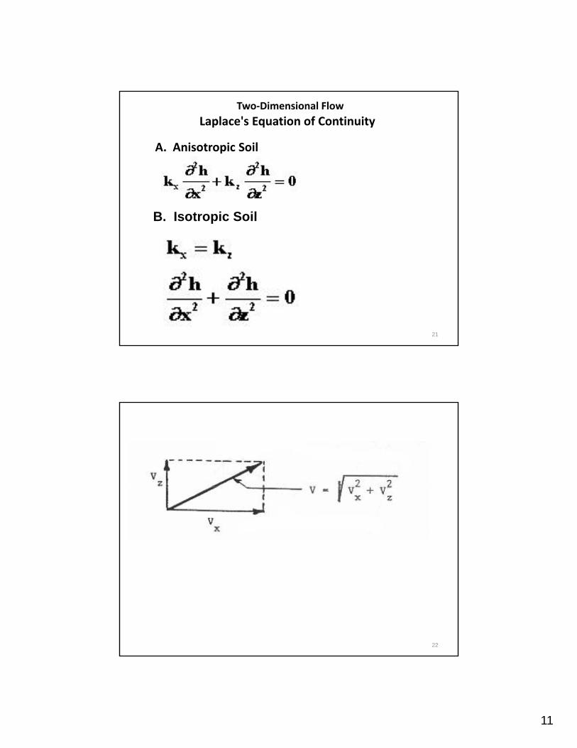
Two‐Dimensional FlowLaplace's Equation of Continuity
A. Anisotropic Soil
B. Isotropic Soil
21
22
12
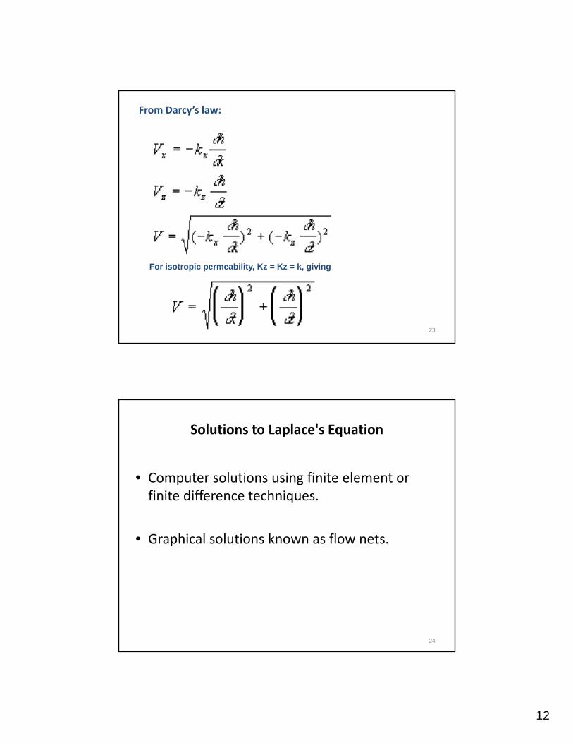
From Darcy’s law:
23
For isotropic permeability, Kz = Kz = k, giving
Solutions to Laplace's Equation
• Computer solutions using finite element or p gfinite difference techniques.
• Graphical solutions known as flow nets.
24
13
Solutions to Laplace's equation for two‐dimensional seepage can be presented as flow nets.
Two orthogonal sets of curves form a flow net:
• flow lines
• equipotentials
25
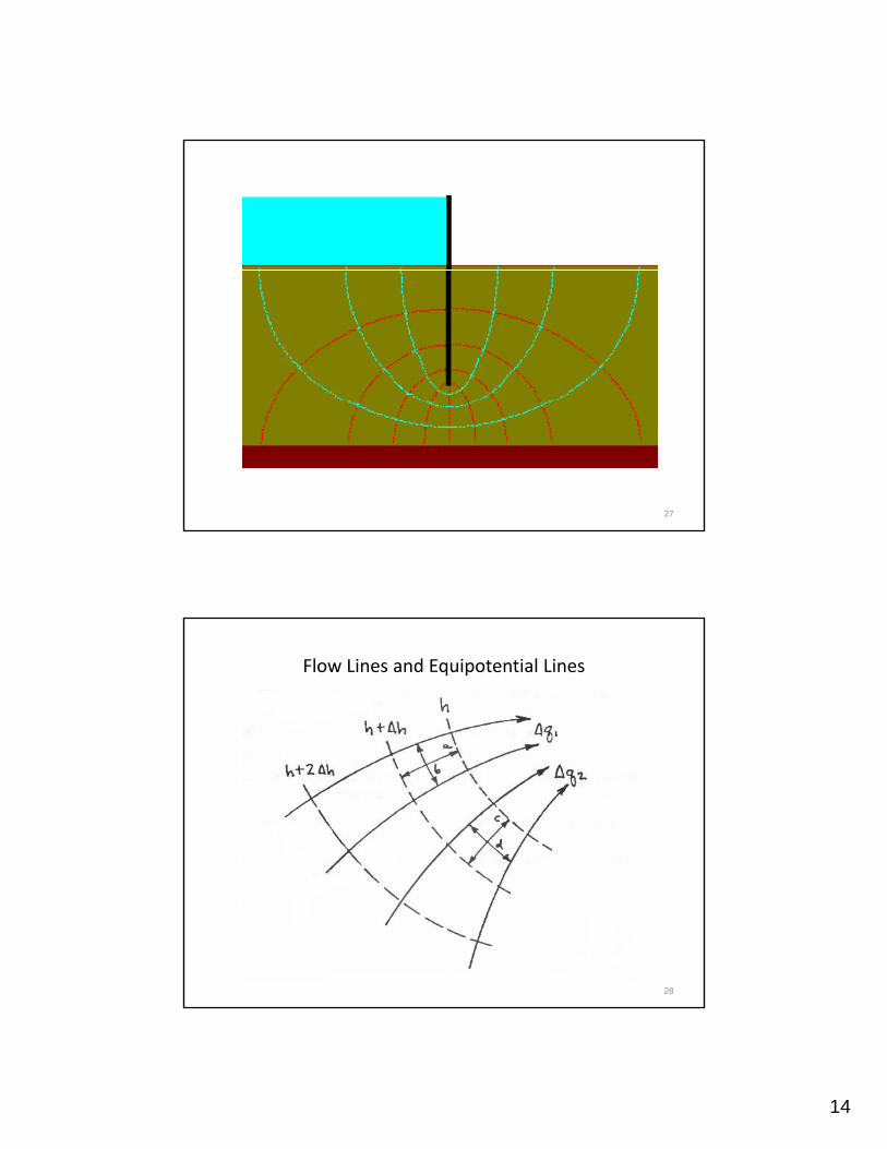
Flow Lines and Equipotential Lines
• A flow line is the path a water particle would follow in moving from upstream to downstream.
• An equipotential line is a line along which the total head, h, is a constant value. It is similar to a contour line, except that total head is constant, rather than elevation.
• A flow net is a combination of flow lines and equipotential lines that satisfy Laplace's equation and the boundary conditions.
26
14
27
Flow Lines and Equipotential Lines
28
15
29
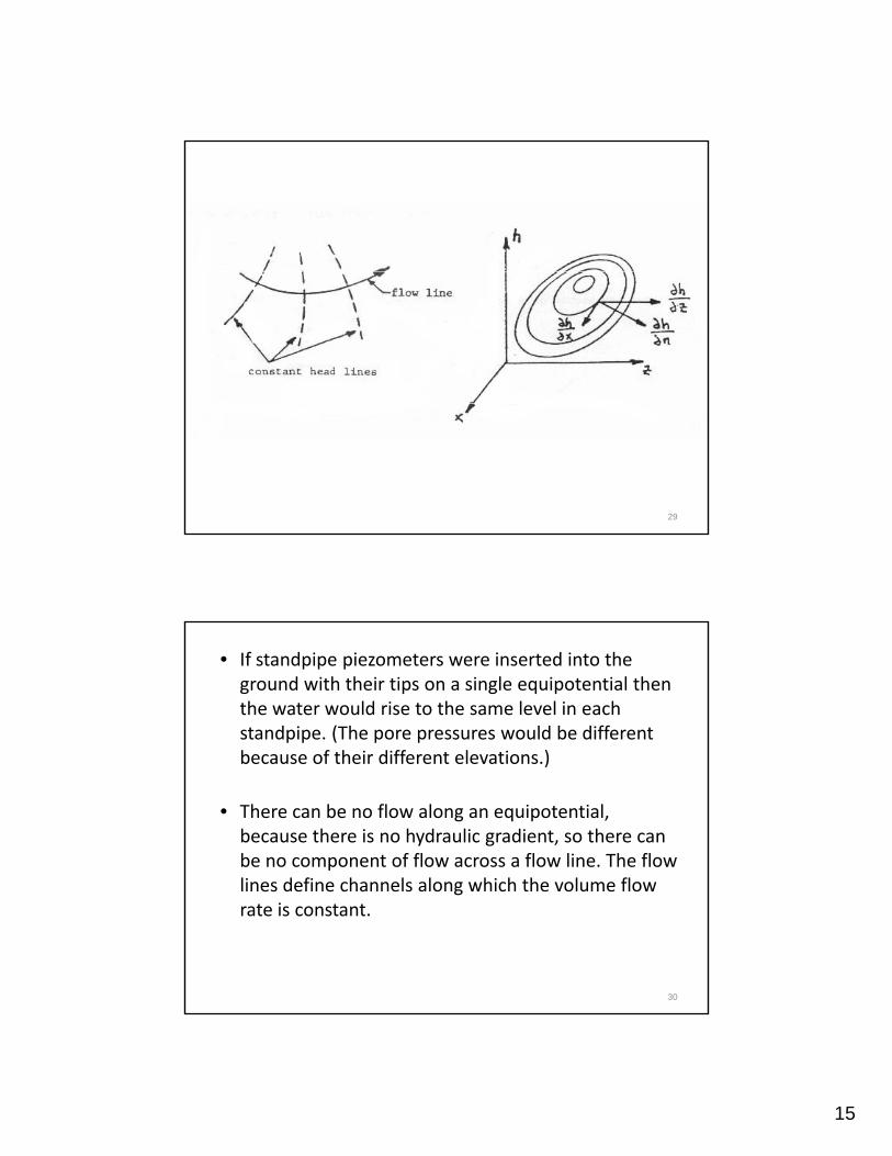
• If standpipe piezometers were inserted into the ground with their tips on a single equipotential then the water would rise to the same level in each standpipe. (The pore pressures would be different b f th i diff t l ti )because of their different elevations.)
• There can be no flow along an equipotential, because there is no hydraulic gradient, so there can be no component of flow across a flow line. The flow lines define channels along which the volume flowlines define channels along which the volume flow rate is constant.
30
16
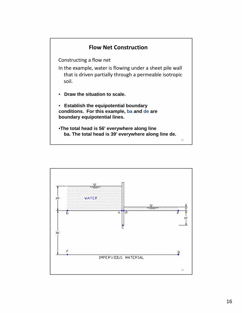
Flow Net Construction
Constructing a flow net
In the example, water is flowing under a sheet pile wall th t i d i ti ll th h bl i t ithat is driven partially through a permeable isotropic soil.
• Draw the situation to scale.
• Establish the equipotential boundary
31
conditions. For this example, ba and de are boundary equipotential lines.
•The total head is 56' everywhere along line ba. The total head is 39' everywhere along line de.
32
17
Rules for Flow Net Construction
• Establish the flow boundary conditions. For this example, acd and fg are boundary flow lines.
• Flow lines and equipotential lines must always intersect at right angles.
• The fields should be "square". By this we mean that the length and width of a field should be equal. Fields are the spaces in a flow net formed by theare the spaces in a flow net formed by the intersecting flow lines and equipotential lines. The sides of the fields are commonly curved, so the term "square" is a stretch of the normal definition.
33
Construction of the Flow Net
• The flow net for this example follows.
• Equipotential lines are red and dashed while flowEquipotential lines are red and dashed, while flow lines are green and solid.
• The length and width of one of the fields is shown.
• The length in the direction of flow is L, while theThe length in the direction of flow is L, while the width is b. To be "square" ( L= b ).
34
18
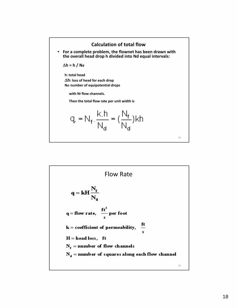
Calculation of total flow• For a complete problem, the flownet has been drawn with
the overall head drop h divided into Nd equal intervals:
Δh = h / Nd
h: total headΔh: loss of head for each dropNd: number of equipotential drops
with Nf flow channels.
Then the total flow rate per unit width is
35
Flow Rate
36

19
Flow Net Calculations
A. Example
• The flow net from the previous section will be pused for the calculations.
• The coefficient of permeability for the soil is 0.04 ft/s
37
38

20
39
For the example:
40
21
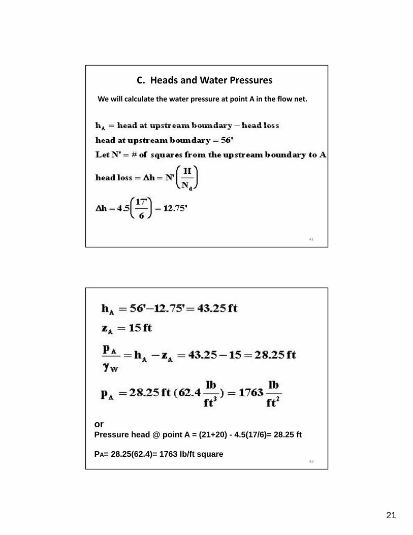
C. Heads and Water Pressures
We will calculate the water pressure at point A in the flow net.
41
42
orPressure head @ point A = (21+20) - 4.5(17/6)= 28.25 ft
PA= 28.25(62.4)= 1763 lb/ft square
22
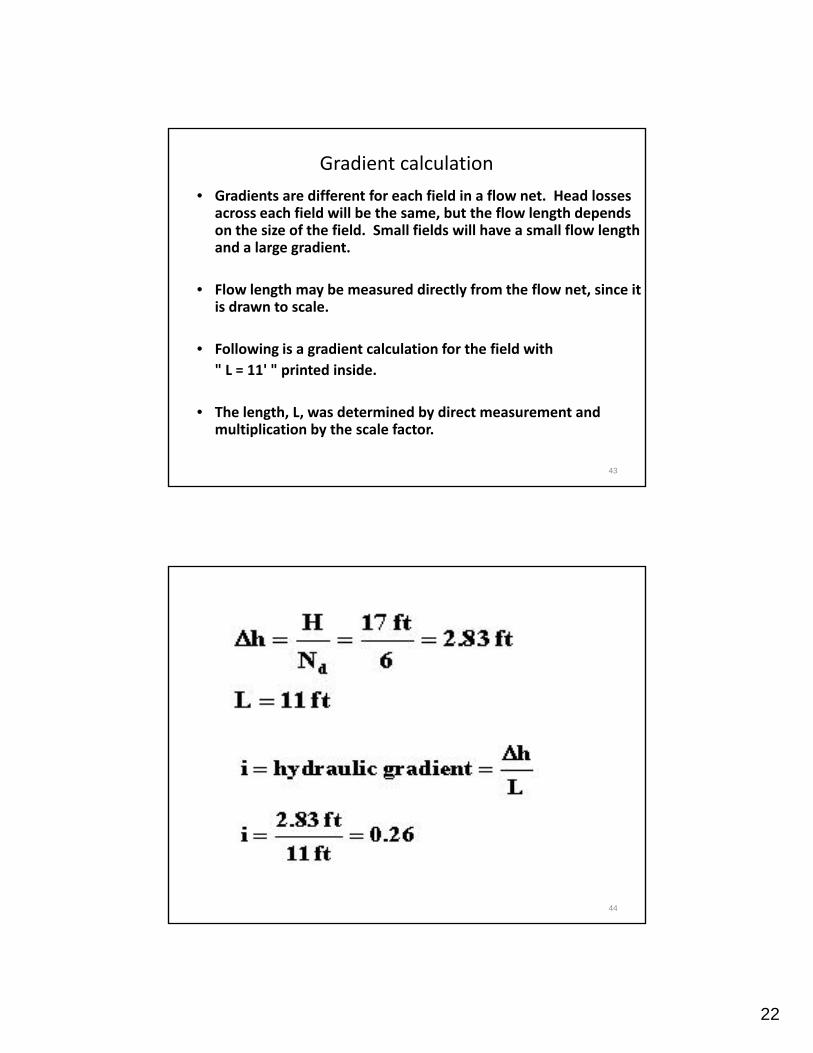
Gradient calculation
• Gradients are different for each field in a flow net. Head losses across each field will be the same, but the flow length depends on the size of the field. Small fields will have a small flow length and a large gradientand a large gradient.
• Flow length may be measured directly from the flow net, since it is drawn to scale.
• Following is a gradient calculation for the field with " L 11' " printed inside" L = 11' " printed inside.
• The length, L, was determined by direct measurement and multiplication by the scale factor.
43
44
23
critical hydraulic gradient (ic)
• The hydraulic gradient at which effective t b ith dstresses becomes zero; with upward seepage, sand may become quicksand.
45
Quick condition and piping
• If the flow is upward then the water pressure tends lif h il l f h dto lift the soil element. If the upward water pressure
is high enough the effective stresses in the soil disappear, no frictional strength can be mobilised and the soil behaves as a fluid.
• This is the quick or quicksand condition and is associated with piping instabilities around excavations and with liquefaction events in or following earthquakes.
46
24
Critical hydraulic gradient
• The quick condition occurs at a critical upward hydraulic gradient ic, when the seepage force j b l h b i h fjust balances the buoyant weight of an element of soil.
47