Embed Size (px)
Citation preview

SCHOOL OF ELECTRONIC, ELECTRICAL AND COMPUER
ENGINEERING
THE UNIVERSITY
OF BIRMINGHAM
INVESTIGATION OF MICROWAVE
TRI-RESONATOR STRUCTURES
Negassa Sori Gerba
A thesis submitted to the University of Birmingham for the degree of Master of
Research in Electronic, Electrical and Computer Engineering
April 2012

University of Birmingham Research Archive
e-theses repository This unpublished thesis/dissertation is copyright of the author and/or third parties. The intellectual property rights of the author or third parties in respect of this work are as defined by The Copyright Designs and Patents Act 1988 or as modified by any successor legislation. Any use made of information contained in this thesis/dissertation must be in accordance with that legislation and must be properly acknowledged. Further distribution or reproduction in any format is prohibited without the permission of the copyright holder.

i
Abstract
In this thesis a clear synthesis technique to design a power splitter based on three
resonators is introduced. A new analytic synthesis method is developed to investigate a
coupled resonator structure with only three resonators and three ports. The general
formulae to calculate the coupling coefficients between resonators are analytically
derived. This method avoids the use of the polynomial synthesis technique.
The mathematical analysis is extended for the realisation of an asymmetric frequency
response of a trisection filter. A simple mathematical function with a minimum number of
parameters is developed which can be used as a cost function when using optimisation.
These parameters are coupling coefficients and external quality factors, and are called
control variables. A coupling matrix optimisation technique is used to obtain optimised
values of control variables to realise an asymmetric frequency response of a trisection
filter. The optimisation algorithms effectively reduce the cost function, and generate
appropriate values of control variables when the function is minimised.

ii
Acknowledgments
Having completed this thesis, I thank the Almighty GOD for keeping me in good health to
accomplish the assignments that were expected of me in this thesis.
During my M.Res study at the University of Birmingham, I have been privileged to have
Professor Mike Lancaster as my supervisor. I would like to thank him for proving me an
opportunity to conduct this M.Res research. I am grateful to him for his patient mentoring,
inspiring suggestions and endless editing.
My deepest gratitude also goes to my wife for her all round support and encouragement
she has provided me throughout the year while studying my M.Res research. She has
endured much sacrifice for the sake of my education. I could not have accomplished what
I did without her boundless love, sacrifice, support, and encouragement.
I would like to extend my thanks to my peers in the Emerging Device Technology (EDT)
research group in general and Dr. Xiobang Shang in particular for providing discussions
on technical issues and suggestions that has always been granted without any hesitation.
Last, but not least, my acknowledgments also goes to UK-Council for Assisting Refugee
Academics (CARA) for covering the cost of my M.Res study.

Dedicated To my Wife
(Genet D Merera)
And
My Children
(Simeera and Hawwera)

iii
Table of Contents
Abstract .............................................................................................................................. i
Acknowledgments .......................................................................................................... ii
Table of Contents .......................................................................................................... iii
Chapter 1: Introduction .................................................................................... 1
1.1. Background ............................................................................................................ 1
1.2. Overview of Power Splitter.................................................................................... 2
1.3. Thesis Overview .................................................................................................... 3
1.4. Thesis Motivation .................................................................................................. 3
1.5. Thesis Outline ........................................................................................................ 4
Chapter 2: Microwave Resonators ............................................................. 6
2.1. Introduction ............................................................................................................ 6
2.2. Lumped Resonant Circuits ..................................................................................... 7
2.2.1. The Quality Factor, Q ..................................................................................... 8
2.2.1.1. Loaded and unloaded Quality Factor, Q...................................................10
Chapter 3: Coupling of Resonator Circuits ........................................ 12
3.1. Introduction .......................................................................................................... 12
3.2. Back Ground Theory of Coupling ....................................................................... 12
3.3. General 3 3 Coupling Matrix Derivation for Tri-resonator Structure .............. 15
3.3.1. Magnetic Coupling ....................................................................................... 15
3.3.2. Electric Coupling .......................................................................................... 25
3.4. Direct and Cross Coupling ................................................................................... 33
Chapter 4: Passive Microwave Circuits ................................................ 36
4.1. Introduction .......................................................................................................... 36
4.2. Passive Filters ...................................................................................................... 37

iv
4.2.1. Power Splitters .............................................................................................. 38
4.2.1.1. Insertion and Reflection Losses..........................................................40
4.2.1.2. Power Splitter Polynomial.......................................................................44
4.3. Coupling matrix Method for Designing Filters.................................................... 46
4.3.1. Derivation of Reflection and Transmission zero locations for a 3x3
Normalised Coupling Matrix....................................................................................... 47
4.3.1.1. Frequency Locations of Transmission zero.......................................40
4.3.1.2. Frequency Locations of Reflection zero............................................40
Chapter 5: Microwave Tri-resonator Filter Structure ................ 57
5.1. 3-dB Tri-resonator Power Splitter Coupling Matrix Synthesis ........................... 57
5.1.1. Design procedure for Power Splitter with no Coupling between
Resonators 2 and 3 ...................................................................................................... 57
5.1.2 Coupling Matrix Power Divider Examples ........................................................ 66
5.2. Trisection Filter .................................................................................................... 71
5.2.1. Analysis ........................................................................................................ 73
5.2.2. Optimisation ................................................................................................. 78
5.2.2.1. Frequency Locations of Transmission zero.......................................79
Chapter 6: Conclusion and Future Work ............................................ 87
6.1. Conclusion ........................................................................................................... 87
6.2. Future Work ......................................................................................................... 89
References .......................................................................................................................... 91
Appendix A ........................................................................................................................ 95
Solution to Polynomial Equation .................................................................................... 95
Appendix B ........................................................................................................................ 97
Calculations of Cofactors and Determinant of the Normalised Coupling Matrix, A .. 97

Chapter-1: Introduction
1
Chapter 1
Introduction
1.1. Background
This review considers methods of calculating coupling matrix and external quality factors
for a coupled resonator filter with multiple ports. Multiport microwave coupled resonator
synthesis has been presented in [11], in addition the two port formulation for n-coupled
resonator filter for both electrically and magnetically coupled resonators has also been
implemented in [1]. In the literature, different methods have been used to extract the
coupling matrix and external quality factors for multi port networks [8]. Coupling matrix
methods of synthesising microwave filters are discussed in chapter 4. For a two-port
network, an optimisation procedure utilizing a mathematical function for the extraction of
coupling coefficients and external quality factors has been proposed in [19].
In the literature, several approaches [1], [2], [11], [12], [17] have been proposed to realise
the frequency response of coupled resonators for different resonator structures. General
tri-resonator filters and their capability of providing both bandpass and band-reject
behaviour has been investigated in [10], however, to my knowledge, the tri-resonator
structure has not been investigated in detail.
The proposed equivalent circuit of a tri-resonator structure is shown in Figure 1.1. The
circuit demonstrate the coupling between adjacent and non-adjacent resonators. A general
coupling theory of resonator circuits and their applications are presented in Chapter 3.

Chapter-1: Introduction
2
Even though a large number of articles dealing with coupling matrix synthesis have
recently been and being published [8], [11], [12], [17], [18], none of them go into details
about how to calculate the coupling parameters of a three port network with only three
resonators by analytic method.
R1
R2C1
i1
i2
C2
L1
L2
es
m13
m23
m12
Resonator 1
Resonator 2
R3i3
C3
L3
Resonator 3
Figure 1.1 Equivalent circuit prototype of Tri-resonator filter structure.
In this thesis, for the realisation of a tri-resonator structure, the values of normalised
coupling coefficients and external quality factors that can realise a required response is to
be calculated analytically. This is attempted without recourse to polynomials.
1.2. Overview of Power Splitter
A power splitter is a three port network that splits incoming signals from an input port into
two paths or channels, dependent on frequency. It is used in multiport networks for the
transmission and reception of signals or channel separation. Power splitters are an RF
microwave accessory constructed with equivalent (often 50Ω) resistance at each port.
These components divide power of a uniform transmission line equally between ports.

Chapter-1: Introduction
3
They provide a good impedance match at both the output ports when the input is
terminated in the system characteristic impedance (usually 50Ω). Once a good source
match has been achieved, a power splitter can be used to divide the output into equal
signals.
1.3. Thesis Overview
By investigating a three resonator structure, looking at the coupling coefficients between
the resonators, simple power splitters are to be investigated. The investigation is based on
the radio frequency (RF) circuit analysis and coupling matrix optimisation techniques to
make the response of coupled tri-resonator structure close to the idealised circuit responses
of the power splitters. The work in this thesis also covers the theory and design of
trisection filter for two-port tri-coupled resonators.
Determination of coupling matrix, m and external quality factors, eiq for 1, 2, 3i of
the three resonators by analytic and coupling matrix optimisation techniques are the main
challenging aspect of this thesis. The thesis will try and determine what specifications of
power splitters are possible with only three resonators.
1.4. Thesis Motivation
There has been an increasing demand in reducing design complexity of microwave
components. The thesis addresses the method to calculate the normalised coupling
coefficients and external quality factors for the design of power splitter without the need to
use optimisation or even polynomials. Thus, it will investigate and develop simple
mathematical formulations to calculate the coupling parameters.
Chapter-1: Introduction
4
In this thesis, assumptions are made during a general 3 3 coupling matrix manipulation
in developing mathematical relations between normalised coupling coefficients and
external quality factors. The reflection zeros for the three port tri-coupled tri-resonator
structures have been specified and used in the analytical equations to reduce the
complexity of mathematical derivations. A 3 dB power splitter is designed using the
calculated normalised coupling coefficients and external quality factors. For the trisection
filter, a general equation with minimum number of parameters to be optimised is
developed from the transmission and reflection scattering parameters. The mathematical
relation developed has only 4 parameters rather than 12 for the full solution. Thus,
optimisation algorithms are only required for four variables.
1.5. Thesis Outline
The organisation of this thesis is as follows:
After the introduction in Chapter 1, chapter 2 looks in to the basics of the microwave
resonators. In this chapter, the basic operations of microwave resonators are briefly
discussed by using lumped resonant circuits. The loaded and unloaded quality factors of
microwave resonators are also discussed briefly.
Chapter 3 describes coupled resonator circuits in conjunction with the coupling theory of
coupled resonators. A detailed derivation of a general 3 3 coupling matrix of tri-coupled
resonators with a three-port network, which will be used in the rest of the thesis, is
presented. A combined relation for the transmission and reflection scattering parameters
are drawn from loop and node equation formulations for magnetically and electrically
coupled resonator circuits, respectively. Cross couplings and direct couplings are
discussed in this chapter to present them in coupling matrix synthesis which is also

Chapter-1: Introduction
5
covered here. A circuit prototype model for the tri-resonator structure and the proposed
coupling structure for the design of power splitter and for the realisation of trisection filter
are demonstrated.
Passive microwave filters such as power splitter theories are presented in chapter 4. The
basics of polynomial synthesis for the two ports and three ports network are briefly
introduced. Coupling matrix method for designing filters is discussed in detail. Lastly in
this chapter, detailed mathematical analysis is carried out to derive mathematical formulae
to calculate transmission and reflection zero locations for the proposed structure.
Chapter 5 describes an analytical design method for tri-resonator power splitters. This
section mainly focuses on developing the analytical design by calculating normalised
coupling coefficients and the scaled external quality factors. A general analysis of the
power splitter is presented, which is to develop a general equation for calculating the
normalised coupling coefficients and the external quality factors of resonators. In deriving
the general formulae, some assumptions are made to simplify the design. To develop a
general formulae, the frequency locations of reflection zeros are specified and used
throughout mathematical analysis to reduce the complexity. Specifying the frequency
locations of reflection zeros, and using them in the general formulae will also reduce the
number of unknown parameters within the equations. A design of a trisection filter can be
achieved by extending this equation; however, in this case optimisation methods are used
as it is not possible to calculate all the required coupling parameters. It is worth
mentioning here that the analytic approach has simplified the equation and reduces the
time taken by the optimisation routine.
The final chapter of the thesis (chapter 6) presents the conclusions and suggested works.
The significance and contribution of this thesis work is summarised in this Chapter.

Chapter-2: Microwave Resonators
6
Chapter 2
Microwave Resonators
2.1. Introduction
Resonators are lumped element networks or distributed circuits that allow the exchange of
electric and magnetic energies with low loss. Lumped elements such as inductors and
capacitors are usually employed for resonators at frequencies below 300 Megahertz
(MHz) [3]. At higher frequencies, the dimensions of the general lumped elements are
comparable to the wavelength in size. Smaller devices are possible with the advantage of
integrated circuit (IC) technology. However, small sizes result in poor power handling
capacity and low quality factors, and this is presented in the subsequent sections.
Therefore, resonators consisting of distributed components are usually constructed for
applications in the microwave frequency range. Distributed resonator circuits utilize the
resonant properties of standing waves and thus are generally of a size comparable to
wavelength. Although lumped circuits are not generally applicable at high frequencies,
they are good models to present the basic operation of all resonators.
In this chapter lumped resonant circuits and microstrip ring resonators are discussed. Ring
resonators can be easily cross coupled with the wide range of coupling coefficients
between resonators. This is presented in chapter 5 for the practical design of tri-resonator
power splitter and trisection filter.

Chapter-2: Microwave Resonators
7
2.2. Lumped Resonant Circuits
A resonant circuit or tuned circuit consists of an inductor, L , a capacitor, C and a resistor,
R in series or parallel. When connected together, they can act as an electrical resonator
storing electrical energy oscillating at the circuits’ resonant frequency.
RLC circuits are used in the generation of signals at a particular frequency, or picking out
a signal at a particular frequency from more complex filters. They are key components in
many applications such as oscillators, filters, tuners and frequency mixers. An LC circuit
is an idealized model since it assumes there is no dissipation of energy due to resistance.
The purpose of an RLC circuit is to oscillate with minimal damping, and for this reason
their resistance is made as low as possible. Even though there is no practical circuit, which
is without losses, it is instructive to study this pure form to gain a good understanding. A
parallel and series RLC lumped element resonator circuits are shown in figure 2.1(a) and
(b) respectively.
C1L1R1
V1
(a)
C2
L2
R2
(b)
V2
Figure 2.1 Resonant circuits (a) parallel and (b) series
Consider the simple parallel resonant circuit shown in figure 2.1 (a). In this case, lumped
elements 1 1 1, and R C L share a common voltage V1. If Ploss is the average power loss in
the resistor R1, Wm the average magnetic energy in the inductor L1 and We the average

Chapter-2: Microwave Resonators
8
electric energy stored in the capacitor C1, the average dissipated power can be expressed
as
2
1
1
1
2loss
VP
R (2.1)
Its input impedance is given by
1 1
1
1Z R j L
j C
(2.2)
At the resonance the input impedance is purely real and equal to R1. Resonance occurs when the
stored average magnetic and electric energies are equal, such as Wm=We. The frequency at which
resonance occurs is referred to as angular resonant frequency 0 , which is defined as
0
1 1
1
L C (2.3)
An important parameter of a resonant circuit is its quality factor, Q and this is discussed in the
following section briefly.
2.2.1. The Quality Factor, Q
The quality factor, Q is a useful measure of sharpness of resonance [3], and also it is used
to measure the loss of resonator circuit. Q can be defined as
time average energy stored in the system
average energy loss per second in the systemQ

Chapter-2: Microwave Resonators
9
As can be seen from this definition, low loss implies a higher quality factor, Q.
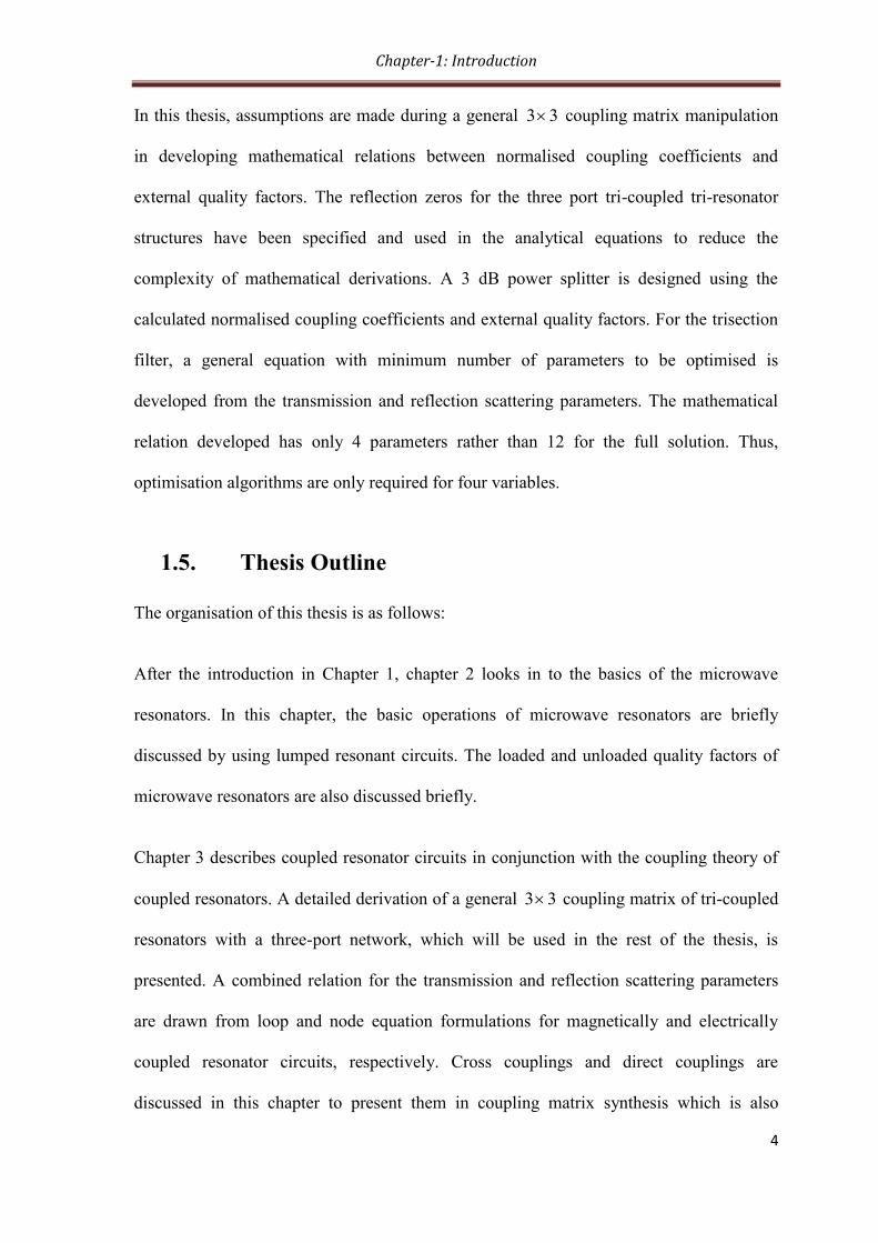
A high Q factor results in a steep roll-off and narrow bandwidth of the resonator [7] as
shown in figure 2.2. At resonance, Q can be expressed in terms of the magnetic and
electric energies stored in lumped element resonators as well as microwave resonators as
[7]
0
m e
loss
W WQ
P
(2.4)
In terms of lumped resonant circuit elements 1 1 1, and R C L , the Q of the parallel resonant
circuit can be evaluated as
1
0 1 1
0 1
RQ R C
L
(2.5)
Thus it can be seen from equation (2.5) that a small value of resistance in an RLC circuit
implies low Q-factor.
Q -factor can also be defined in terms of resonance frequency 0 and bandwidth of
the response of the resonator circuit as
0 0
2 1
Q
(2.6)

Chapter-2: Microwave Resonators
10
where 0 is the angular resonant frequency and 2 1 is the 3-dB bandwidth
Transmitted
power in
dB
-3dB
Frequency01 2
Figure 2.2 Graph of Q -factor
2.2.1.1. Loaded and Unloaded Quality Factor, Q
The quality factor defined in the previous section is in the absence of any loading effects
caused by external circuitry, and it is the characteristic of the resonant circuit itself and is
called unloaded uQ . The unloaded quality factor, uQ involves the power loss by resonant
circuit only. In practice, a resonant circuit is coupled to external circuitry, which dissipates
additional power denoted by eP . The external Q factor denoted by eQ is defined in terms
of the power dissipated in the external circuitry, and magnetic energy, Wm and electric
energy, We stored in inductor L1 and capacitor C1 respectively as
0
m e
e
e
W WQ
P
(2.7)
Similarly, the Q factor of the loaded resonator, QL
associated with the total loss can be
expressed as
0
m e
L
loss e
W WQ
P P
(2.8)
Chapter-2: Microwave Resonators
11
Looking at equation (2.8), it is clear that the effect of the external load always lowers the
overall Q factor of a resonator.
Using equations (2.4), (2.7) and (2.7), the relationship between QL, Qu and Qe can be
shown as
1 1 1
L u eQ Q Q
(2.9)
The degree of coupling between the external circuit and resonant circuit is measured by
coupling coefficient k, and in general, k can be defined in terms of the Q factor as [7]
or u u L
e L
Q Q Qk k
Q Q
(2.10)
The coupling coefficient k denotes the ratio of the power dissipated in the external circuit
to the power loss in the resonant circuit itself. For the condition k=1, the coupling is
referred to as critical coupling. If k >1, the resonator is said to be over coupled and k<1 is
called under coupled [9].

Chapter-3: Coupling of Resonator Circuits
12
Chapter 3
Coupling of Resonator Circuits
3.1. Introduction
For the design of RF/microwave filters, coupling of resonator circuits is one of the most
significant factors affecting filter performance. A set of microwave resonators electrically
and/or magnetically coupled to each other and coupled to an external feed circuit are used
to realize a filter. The number and the type of the couplings between the resonators
determine the overall performance of the device [1]. Design techniques are extended in
this thesis to a three-port network having a single input and two output port circuits such
as a power splitter. The general coupling matrix of a two-port n-coupled resonator filter is
formulated in detail in [1]. Based on the principle in [1], the general coupling matrix of a
three-port tri-coupled resonator is derived, and its relation to the scattering parameters is
presented in the next sections. For the design of power splitter, this thesis is mainly based
on the general formulae of scattering parameters in terms of normalised coupling matrix
derived in this section.
3.2. Back Ground Theory of Coupling
A general technique for designing coupled resonator filters is based on coupling
coefficients of inter- coupled resonators and the external Q -factors of the input and output
resonators [1].
The coupling coefficient, k , of two coupled microwave resonators as shown in figure 3.1

Chapter-3: Coupling of Resonator Circuits
13
can be defined on the basis of the ratio of coupled energy to stored energy, and it can be
defined mathematically as [1]
1 2 1 2
122 22 2
1 2 1 2
E E dv H H dvk
E dv E dv H dv H dv
(3.1)
where 1E and 2E are the electric fields in resonator 1 and 2, respectively, and 1H and 2H
are the magnetic fields in resonator 1 and 2, respectively.
coupling
1
2
HH
1
2
EE
Resonator 1 Resonator 2
Figure 3.1 General coupled microwave resonators where resonators 1 and 2 can have
different structure and have different resonant frequencies [1].
Mathematically, the dot operation of the space vector describes the interaction of the
coupled resonator as shown in equation (3.1). This allows the coupling to have either
positive or negative sign. A positive sign would imply that the coupling enhances the
stored energy of uncoupled resonators, whereas a negative sign indicates that coupling
reduces the stored energy of uncoupled resonator. Therefore, the electric and magnetic
coupling could either have same effect if they have the same sign, or have the opposite
effect if their signs are opposite [1].

Chapter-3: Coupling of Resonator Circuits
14
The typical resonant response of a coupled resonator is shown in figure 3.2. The
magnitude of the coupling coefficient defines the separation d of the two resonance peaks
as in Figure 3.2.
Normally, the stronger the coupling, the wider separation d of the two resonance peaks,
and the deeper the trough is in the middle [1].
1 2 Frequency
d
Am
pli
tude
(dB
)
Figure 3.2 Resonant response of coupled resonator structure [1]
For a pair of synchronously tuned resonators, the coupling coefficient in terms of 1 and
2 is defined as in [31]
2 2
2 1
2 2
2 1
k
(3.2)
where 1 and 2 are lower and upper cut-off angular frequencies, respectively.
As 2 f , equation (3.2) can be more simplified as
2 2
2 1
2 2
2 1
f fk
f f
(3.3)

Chapter-3: Coupling of Resonator Circuits
15
Equation (3.3) can be used for both magnetic and electric coupling calculations [1], but the
phase of 21S must be taken into account to get the sign of k . Magnetic and electric
coupling of resonators will be discussed in the next section.
3.3. General 3 3 Coupling Matrix Derivation for Tri-resonator
Structure
The equivalent circuit description for a three-port network of tri-coupled resonator
structure is shown in figure 3.3. In the subsequent sections, the equivalent circuit of
magnetically and electrically coupled resonators with only three resonators is considered
in the derivation of a 3 3 coupling matrix. The reflection and transmission scattering
parameters in terms of this coupling matrix for the magnetically coupled and electrically
coupled resonators are also generalised and incorporated into one form.
3.3.1. Magnetic Coupling
Energy may be coupled between adjacent resonators by either an electric or a magnetic or
both. Figure 3.3 shows the equivalent circuit of three resonators coupled to each other with
mutual inductances linking each inductor.
The impedance matrix for magnetically n-coupled or the admittance matrix for electrically
n- coupled resonators for the two port network is formulated in [2]. The coupling matrix
of n - coupled resonators in an N-port network is obtained from the equivalent circuit of n-
coupled resonators in [2]. A general normalised coupling matrix A in terms of coupling
coefficients and external quality factors for any coupled resonator structure with multiple
outputs has been derived in [2]. Using loop equation formulation used in [1] for the
magnetically coupled resonator, a normalised coupling matrix A can be derived from a

Chapter-3: Coupling of Resonator Circuits
16
tri-coupled tri-resonator structure shown in figure 3.3. Figure 3.3 depicts a low-pass circuit
prototype of tri-coupled resonators, where L , R and C denote the inductance, resistance
and capacitance, respectively. se represents the voltage source and i is the loop current
flowing in each resonator, and 12L , 13L and 23L represent the mutual inductances between
resonators 1 and 2, resonators 1 and 3 and resonators 2 and 3, respectively.
C3
L3
R3
C2
L2
R2
C1
L1
R1
esi2i1
L12
L23
L13
i3
Figure 3.3 Equivalent circuit prototype of magnetically tri-coupled tri-resonator structure
having three ports operating between source impedance 1R , representing port 1 and load
impedances 2R and 3R , representing ports 2 and 3 respectively.
The circuit is driven by a source of open-circuit voltage se with resistance 1R and
terminated by load impedances 2R and 3R . Each loop is coupled to every other loop
through mutual couplings and these couplings are assumed to be frequency-independent
due to the narrow-band approximation [20].
To write the loop equations of the equivalent circuit shown in figure 3.3, Kirchhoff’s
voltage law (or Kirchhoff’s loop rule) can be used. Kirchhoff’s law states that the total

Chapter-3: Coupling of Resonator Circuits
17
voltage around a closed loop must be zero. Therefore, the loop equations for figure 3.3 can
be written as
1 1 1 11 1 12 2 13 3
1
21 1 2 2 2 22 2 23 3
2
31 1 3 3 3 33 3 32 2
3
1
10
10
sR j L i j L i j L i j L i ej C
j L i R j L i j L i j L ij C
j L i R j L i j L i j L ij C
(3.4)
where ij jiL L represents the mutual inductance between resonators i and j where i =1,
2, 3 and j =1, 2, 3. A voltage-current relationship for each loop in equation (3.4) can be
combined into the matrix form as
1 1 11 12 13
11
21 2 2 22 23 2
2
3
31 32 3 3 33
3
1
10
01
s
R j L j L j L j Lj C
e i
j L R j L j L j L ij C
i
j L j L R j L j Lj C
(3.5)
Equation (3.5) can be expressed as
se Z i
where Z is a 3 3 impedance matrix.

Chapter-3: Coupling of Resonator Circuits
18
Since all series resonators have the same resonant frequency, the filter of the equivalent
circuit model in figure 3.3 is synchronously tuned. If all resonators are synchronously
tuned, they would resonate at the same resonant frequency, 0 given by
0
1
LC
where 1 2 3L L L L and 1 2 3C C C C
The impedance matrix in equation (3.5) can be expressed by
0. . .Z L FBW Z
(3.6)
where FBW is the fractional bandwidth of filter and given by 0FBW , and Z
is
the normalised impedance matrix shown as
0. .
ZZ
L FBW
(3.7)
Equation (3.7) may be written in more expanded form as
1311 12
0 0 0
2321 22
0 0 0
31 32 33
0 0 0
. . . . . .
. . . . . .
. . . . . .
ZZ Z
L FBW L FBW L FBW
ZZ ZZ
L FBW L FBW L FBW
Z Z Z
L FBW L FBW L FBW

Chapter-3: Coupling of Resonator Circuits
19
131 12
0 0 0
2321 2
0 0 0
31 32 3
0 0 0
. . . . . .
. . . . . .
. . . . . .
j LR j Lp
L FBW L FBW L FBW
j Lj L RZ p
L FBW L FBW L FBW
j L j L Rp
L FBW L FBW L FBW
(3.8)
Defining p as a complex lowpass frequency variable, and given by
0
, for 1, 2, 3. .
iiiZ R
p iL FBW
1 11
01 1 11
0 0 1 0
1
. . =
. . . . . .
j L j LL FBWj C j L j L
L FBW L FBW j C L FBW
0
0
1 -p j
FBW
Defining the external quality factors, 0 1,2,3ei iQ L R of the three resonators shown in
Figure 3.3 for i=1, 2, 3 and the coupling coefficient, ij ijM L L and assuming
0 1 for a narrow-band approximation, equation (3.8) can be simplified as
12 13
1
21 23
2
31 23
3
1
1
1
e
e
e
p jm imq
Z jm p jmq
jm jm pq
(3.9)

Chapter-3: Coupling of Resonator Circuits
20
Where 1 2 3, are e e eq q q are normalised external quality factors given by .ei eiq Q FBW , for
1, 2,3i and ijm is the normalised coupling coefficient and given by
ij
ij
Mm
FBW (3.10)
For the case that the coupled resonators are asynchronously tuned, the circuit prototype in
figure 3.3 can be modified by including the self couplings 11m , 22m and 33m as shown in
figure 3.4.
R
C2
L 1es C 3
L3
1
R 2C1i2L2
m13
m23
m12
Resonator 1
Resonator 2
R 3i3
Resonator 3
m22
m11
m33
i1
Figure 3.4 A circuit prototype for asynchronously tuned tri-coupled tri-resonator filter
showing self couplings.
Thus, the normalised impedance matrix for the asynchronously tuned filters can be shown
as

Chapter-3: Coupling of Resonator Circuits
21
11 12 13
1
21 22 23
2
31 23 33
3
1
1
1
e
e
e
p jm jm jmq
Z jm p jm jmq
jm jm p jmq
(3.11)
Asynchronously tuned coupled resonators indicate that there is a self coupling between
each resonator, represented by a non-zero coupling coefficient, iim for i in this case is 1, 2
and 3. The concept of coupling coefficient is further discussed in section 3.4 when we
discuss inter-resonator coupling and cross-coupling of resonators.
3-port tri-coupled
resonator network
R2
R1
es
R3
V1
V2
V3
a2
a3
I2
I3
I1a1
b1
b3
b2port 1
port 2
port 3
Figure 3.5 Network representation of an equivalent 3-port tri-coupled resonator circuit
shown in figure 3.3, where 1 2 3 1 2 3, , and , ,a a a b b b are wave variables representing incident
and reflected waves, respectively.

Chapter-3: Coupling of Resonator Circuits
22
Now consider the wave variables shown in figure (3.5). From the transmission line theory,
the incident and reflected waves are related by [9]
for 1, 2, 3,....nn
i ij j
j
b S a i (3.12)
where
th, is the reflection coefficient of the i port if with all other ports matched
th, is the forward transmisson coefficient of the j port if with all other ports
matched
, i
S i jij ij
S T i jij ij
S Tij ij
ths the reverse transmission coefficient of the j port if with all all other
ports matched
i j
In general, for n=3, equation (3.12) can be written as
1 11 1 12 2 13 3
2 21 1 22 2 23 3
3 31 3 32 2 33 3
b S a S a S a
b S a S a S a
b S a S a S a
(3.13)
Equation (3.13) may be described in matrix form as
1 111 12 13
2 21 22 23 2
31 32 333 3
b aS S S
b S S S a
S S Sb a
(3.14)
Chapter-3: Coupling of Resonator Circuits
23
The relationship between , , and a b V I are given by [9]
1 1,
2 2
i i
n i i n i i
i i
V Va R I b R I
R R
for i=1,2,…n (3.15)
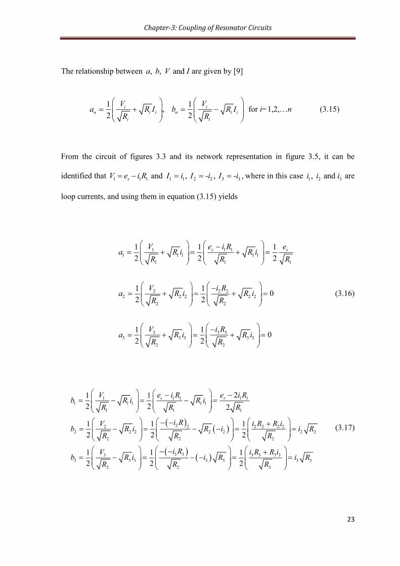
From the circuit of figures 3.3 and its network representation in figure 3.5, it can be
identified that 1 1 1sV e i R and 1 1 2 2 3 3, - , -I i I i I i , where in this case 1 2 3, and i i i are
loop currents, and using them in equation (3.15) yields
1 11
1 1 1 1 1
1 1 1
2 2 22 2 2 2 2
2 2
3 3 3
3 3 3 3 3
2 2
1 1 1
2 2 2
1 10
2 2
1 10
2 2
s se i R eVa R i R i
R R R
V i Ra R i R i
R R
V i Ra R i R i
R R
(3.16)
1 1 1 11
1 1 1 1 1
1 1 1
22 2 2 2 2 2
2 2 2 2 2 2 2
2 2 2
3 33 3 3 3 3
3 3 3 3 3
2 2 3
21 1
2 2 2
1 1 1
2 2 2
1 1 1
2 2 2
s se i R e i RVb R i R i
R R R
i RV i R R ib R i R i i R
R R R
i RV i R R ib R i i R
R R R
3 3i R
(3.17)

Chapter-3: Coupling of Resonator Circuits
24
Substituting equations (3.16) and (3.17) into equation (3.14) yields
1 1
1 111 12 13
2 2 21 22 23
31 32 333 3
2 1
2 2
0
0
s se i R e
R RS S S
i R S S S
S S Si R
(3.18)
From equation (3.18), the Scattering parameters 11 21, S S and 31S for a three port network
can be evaluated at 2 3 0a a as
2 3
2 3
2 3
1 11 1 111 0
1
2 1 2221 0
1
3 1 3331 0 31
1
2 21
2
2
sa a
s s
a a
s
a a
s
e i Rb i RS
a e e
i R RbS
a e
i R RbS S
a e
(3.19)
From equation (3.6) and (3.7), the loop current i is worked out as
1
00
1 1 1
1 2 311 21 31
0 0 0
. .. . .
, ,. . . . . .
s s
ij
ij
s s s
e ei Z
L FBWL FBW Z
e e ei Z i Z i Z
L FBW L FBW L FBW
(3.20)

Chapter-3: Coupling of Resonator Circuits
25
Making use of 0 1,2,3ei iQ L R , .ei eiq Q FBW and equation (3.20) into (3.19) we get
1
1111
1
1
2121
1 2
1
3131
1 3
21
12
12
e
e e
e e
S Zq
S Zq q
S Zq q
(3.21)
3.3.2. Electric Coupling
This section describes the derivation of 3 3 coupling matrix of electrically coupled tri-
resonator structure with three ports, where in this case the electric coupling is represented
by capacitor. In a similar way to the normalised impedance matrix Z
obtained in section
3.3.1 above, the normalised admittance matrix Y
will be derived in this section.
Electrically tri-coupled tri-resonator circuit is shown in figure 3.6, where iv for i =1, 2
and 3 denotes the node voltage, iG for i =1, 2 and 3 represents ports conductance, si is
the source current and 12C , 13C and 23C represent the mutual capacitances across
resonators 1 and 2, resonators 1 and 3 and resonators 2 and 3, respectively. Energy may be
coupled between adjacent resonators by electric coupling. To compute the node equations,
Kirchhoff’s current law is applied to the equivalent circuit prototype of tri-resonator
circuit shown in Figure 3.6. This law states that the algebraic sum of currents leaving a
node in a network is zero. The node voltage equations are formulated as

Chapter-3: Coupling of Resonator Circuits
26
1 1 1 11 1 12 2 13 3
1
21 1 2 2 2 22 2 23 3
2
31 1 3 3 3 33 3 32 2
3
1
10
10
sG j C v j C v j C v j C v ij L
j C v G j C v j C v j C vj L
j C v G j C v j C v j C vj L
(3.22)
Equation (3.22) can be expressed in matrix form as
1 1 11 12 13
11
21 2 2 22 23 2
2
3
31 32 3 3 33
3
1
10
01
s
G j C j C j C j Cj L
i v
j C G j C j C j C vj L
v
j C j C G j C j Cj L
(3.23)
or equivalently .i Y v , where Y is admittance matrix.
is
C1
G1
G2
v2
C11
C13
C23
v1
C2
G3
v3
C3
L2
L3
L1
Figure 3.6 Equivalent circuit prototype of electrically coupled tri-resonator having three
ports operating between source conductance 1G and load conductance 2G and 3G

Chapter-3: Coupling of Resonator Circuits
27
If all resonators are synchronously tuned at the same resonant frequency of
1
0 LC
, where 1 2 3 1 2 3 and C=L L L L C C C , the admittance matrix Y can
be expressed by
0. .Y C FBW Y
(3.24)
where FBW is the fractional bandwidth, and Y
is the normalised admittance matrix.
From equation (3.24), the admittance matrix can be expressed as
1311 12
0 0 0
2321 22
0 0 0 0
31 32 33
0 0 0
. . . . . .
. . . . . . . .
. . . . . .
YY Y
C FBW C FBW C FBW
YY YYY
C FBW C FBW C FBW C FBW
Y Y y
C FBW C FBW C FBW
3-port tri-coupled
resonator network
G2
G1is
G3
V1
V2
V3
a2
a3
I2
I3
I1a1
b1
b3
b2
port 1
port 2
port 3
Figure 3.7 Network representation of 3-port tri-coupled resonator in figure 3.6 where
1 2 3 1 2 3, , and , , a a a b b b are wave variables representing incident and reflected waves,
respectively.

Chapter-3: Coupling of Resonator Circuits
28
131 12
0 0 0
2321 2
0 0 0
31 32 3
0 0 0
. . . . . .
. . . . . .
. . . . . .
j CG j Cp
C FBW C FBW C FBW
j Cj C GY p
C FBW C FBW C FBW
j C j C Gp
C FBW C FBW C FBW
(3.25)
where p is the complex lowpass frequency variable as defined in the previous section.
Defining the external quality factors, 0 1,2,3ei iQ C G of the three resonators shown in
figure 3.6 for i=1, 2, 3 and the coupling coefficient, ij ijM C C and assuming
0 1 for a narrow-band approximation, equation (3.25) can be simplified as
12 13
1
21 23
2
31 23
3
1
1
1
e
e
e
p jm jmq
Y jm p jmq
jm jm pq
(3.26)
Where 1 2 3, are e e eq q q are normalised external quality factors given by .ei eiq Q FBW , for
i=1, 2, 3 and ijm is the normalised coupling coefficient given in equation (3.10).
For asynchronously tuning, where all resonators may resonate at different frequency,
normalised admittance matrix, Y
contains an additional entries 11 22 33, and m m m on the
main diagonal, which accounts for self coupling of each resonator to itself, and is

Chapter-3: Coupling of Resonator Circuits
29
analogous to the normalised impedance of asynchronously tuned resonators shown in
equation (3.11), and given by
11 12 13
1
21 22 23
2
31 23 33
3
1
1
1
e
e
e
p jm jm imq
Y jm p jm jmq
jm jm p jmq
(3.27)
To derive the three-port S-parameters of a tri-coupled resonator, the wave variables in the
three-port network representation in figure 3.7 are related to voltage and current variables,
nV and nI as in equation (3.28). The relationship between , , and a b V I in figure 3.6 can
be derived from equation (3.14) by replacing 1 nG for nR , and expressed as
1
2
1
2
n
n n n
n
n
n n n
n
Ia V G
G
Ib V G
G
for n=1,2, 3 (3.28)
By inspecting the circuit of figure 3.6, and its network representation in figure 3.7, one can
identify that 1 1 2 2 3 3, , V v V v V v and 1 1 1sI i v G , where 1v , 2v and 3v are node
voltages at resonators 1, 2 and 3, respectively, and thus equation (3.28) can be simplified
to

Chapter-3: Coupling of Resonator Circuits
30
1 1 1 1 1 111 1 1 1 1
1 1 1
1 1 1
2 2 2
s si v G e v G G vIa V G V G
G G G
1 2 3
1
1, 0, 0
2
sia a aG
(3.29)
Similarly from
1,
2
n
n n n
n
Ib V G
G
we obtain the reflected wave variables 1 2 3, and b b b as shown in equation (3.30)
1 11 2 2 2 3 3 3
1
2, ,
2
sv G ib b v G b v G
G
(3.30)
Substituting equations (3.29) and (3.30) into equation (3.18) yields
1 1
1 111 12 13
2 2 21 22 23
31 32 333 3
2 1
2 2
0
0
s sv G i i
G GS S S
v G S S S
S S Sv G
(3.31)
From equation (3.31) the S-parameters can be derived as

Chapter-3: Coupling of Resonator Circuits
31
2 3
2 3
2 3
1 11 1 1
11 0 11
1
2 1 22
21 0
1
3 1 33
31 0
1
2 2, 1
2
2
s
a a
s s
a a
s
a a
s
v G ib v GS S
a i i
v G GbS
a i
v G GbS
a i
(3.32)
By combining equations (3.23) and (3.24), the node voltage v can be obtained as
1
00
1 1 1
1 2 311 21 31
0 0 0
. .. . .
, ,. . . . . .
s s
ij
ij
s s s
i iv Y
C FBWC FBW Y
i i iv Y v Y v Y
C FBW C FBW C FBW
(3.33)
Substitution of equation (3.33) into (3.32), and making use of 0ei iQ C G and
.ei eiq Q FBW for 1, 2 and 3i into (3.32) yields
1
1111
1
1
2121
1 2
1
3131
1 3
21
12
12
e
e
e
S Yq
S Yq q
S Yq q
(3.34)
From the derivations in previous and this section, for magnetic and electric coupling of a
general 3 3 coupling matrix of magnetically and electrically coupled tri-resonator

Chapter-3: Coupling of Resonator Circuits
32
structure for three-port network, the normalised impedance matrix for magnetically
coupled and admittance matrix of electrically coupled resonators are identical. Therefore,
the S-parameters of a three-port network of a tri-coupled tri-resonator structure in
equations (3.21) and (3.34) can be incorporated into one form as
1
1111
1
1
2121
1 2
1
3131
1 3
21
12
12
e
e e
e e
S Aq
S Aq q
S Aq q
(3.35)
with A q p U j m , where U is a 3 3 identity matrix, q is a 3 3 matrix
with all entries zero except for 1
11
1
eqq , 22
2
1
e
and 33
3
1
e
, m is the general 3 3
normalised coupling matrix [1].
The extension of the general S-parameters shown in equation (3.35) for the synthesis of a
three-port coupled resonator power splitter is discussed in the next subsequent chapters in
detail.
The thesis realises the proposed tri-coupled resonator structures by developing
mathematical relations to calculate the normalised coupling coefficients, m and external
quality factor, eq at the input and output ports. This is one of the principal aims of this
work. From S-parameters of a three-port network in equation (3.35), a mathematical

Chapter-3: Coupling of Resonator Circuits
33
analysis is extended to derive general equations to compute coupling parameters so that a
power splitter is analysed and designed.
3.4. Direct and Cross Coupling
To demonstrate the concept of direct coupling between adjacent resonators and the cross
coupling between nonadjacent resonators, the bandpass circuit prototype shown in figure
3.8 is used.
The normalised coupling matrix, m for a tri-resonator filter is a 3 3 symmetric matrix,
i.e., Tm m , or ij jim m where the normalised coupling coefficients, ijm represent the
values of couplings between the resonators of the bandpass filter. The coupling
coefficients are the ratio of the coupled to the stored electromagnetic energies and may
take either a positive or negative sign. A negative sign indicates that the coupling
decreases the stored energy of the uncoupled resonators and a positive sign indicates that it
increases [1]. For a normalised coupling matrix m , which is a 3 3 symmetric coupling
matrix is given by
12 13
21 23
31 23
0
0
0
m m
m m m
m m
In the case of synchronously tuned resonators (and symmetric frequency responses), the
values of the coupling coefficients on the main diagonal ( iim ) are always zero. The sub-

Chapter-3: Coupling of Resonator Circuits
34
diagonal entries ( 12m and 23m ) are direct (or sequential) couplings between adjacent
resonators.
R1
R2C1
i1
i2
C2
L1
L2
es
m13
m23
m12
Resonator 1
Resonator 2
R3i3
C3
L3
Resonator 3
Figure 3.8 A bandpass circuit prototype for a tri-coupled tri-resonator filter.
The couplings between all non-sequentially numbered resonators are said to be cross-
couplings. The purpose of cross-coupling in filter design is for the reduction of the
coupling matrix so as to minimise the number of resonators to be coupled. For a bandpass
filter of the kind in figure 3.7, the cross coupling would occur only between resonators 1
and 3, and represented by 13m .
As mentioned in previous section, asymmetric filter frequency response (or
asynchronously tuned filter) has non-zero entries on the main diagonal of the normalised
coupling matrix, m , and are self coupling. The self coupling account for differences in
the resonant frequencies of the different resonators. A 3 3 asymmetric coupling matrix is
given as

Chapter-3: Coupling of Resonator Circuits
35
11 12 13
21 22 23
31 23 33
m m m
m m m m
m m m
where 11m , 22m and 33m are self-coupling coefficients.

Chapter-4: Passive Microwave Circuits
36
Chapter 4
Passive Microwave Circuits
4.1. Introduction
Microwave circuits are composed of distributed elements with dimensions such that the
voltage and phase over the length of the device can vary significantly [3]. They can also
be lumped elements. By modifying the lengths and dimensions of the device, the line
voltage, current amplitude and phase can be effectively controlled in such away to obtain a
specifically desired frequency response of the device [3].
A microwave filter is a two-port microwave circuit whose frequency response provides
transmission at desired frequencies and attenuation at other frequencies. An ideal filter
should perform this function without adding or generating new frequency components,
while at the same time having a linear phase response.
The microwave filter is a vital component in a huge variety of electronic systems;
including mobile radio, satellite communications and radar. They find their use in excess
of applications in areas of wireless communications, wireless networking, digital
communications, target detection and identification, imaging, deep space communications,
medical imaging and treatment, and radio spectrometry [28].
Such components are used to select or reject signals at different frequencies. Although the
physical realisation of microwave filters may vary, the circuit network theory is common
to all.

Chapter-4: Passive Microwave Circuits
37
In the next section passive microwave circuits such as power splitters will be presented,
and a practical filter design using coupling matrix synthesis is demonstrated. It is also
shown that coupling matrix synthesis may be used to have a better understanding and
examine the various calculated filter responses.
4.2. Passive Filters
Passive filters, often consisting of only two or three components are used to reduce
(attenuate) the amplitude of signals. They are frequency selective, so they can reduce the
signal amplitude at some frequencies without affecting others. To indicate the effect a
filter has on wave amplitude at different frequencies, a frequency response graph is shown
in Figure 4.1. This graph plots the loss (on the vertical axis) against the frequency of a
passive filter, and shows the relative output levels over a band of different frequencies.
-10 -8 -6 -4 -2 0 2 4 6 8 10-50
-45
-40
-35
-30
-25
-20
-15
-10
-5
0
Normalised frequency (rad/sec)
Loss
in d
B
Figure 4.1 Passive filter responses
Chapter-4: Passive Microwave Circuits
38
Passive filters only contain components such as capacitors and inductors. This means that,
the signal amplitude at a filter output cannot be larger than the input. Passive filters do not
require any external power supply and are adequately used in many applications.
4.2.1. Power Splitters
Power splitters are passive circuits with a paramount importance in signal splitting and
combining. As mentioned in previous section, they are widely used in base stations,
antenna arrays, and generally in building wireless communication systems and signal
processing applications.
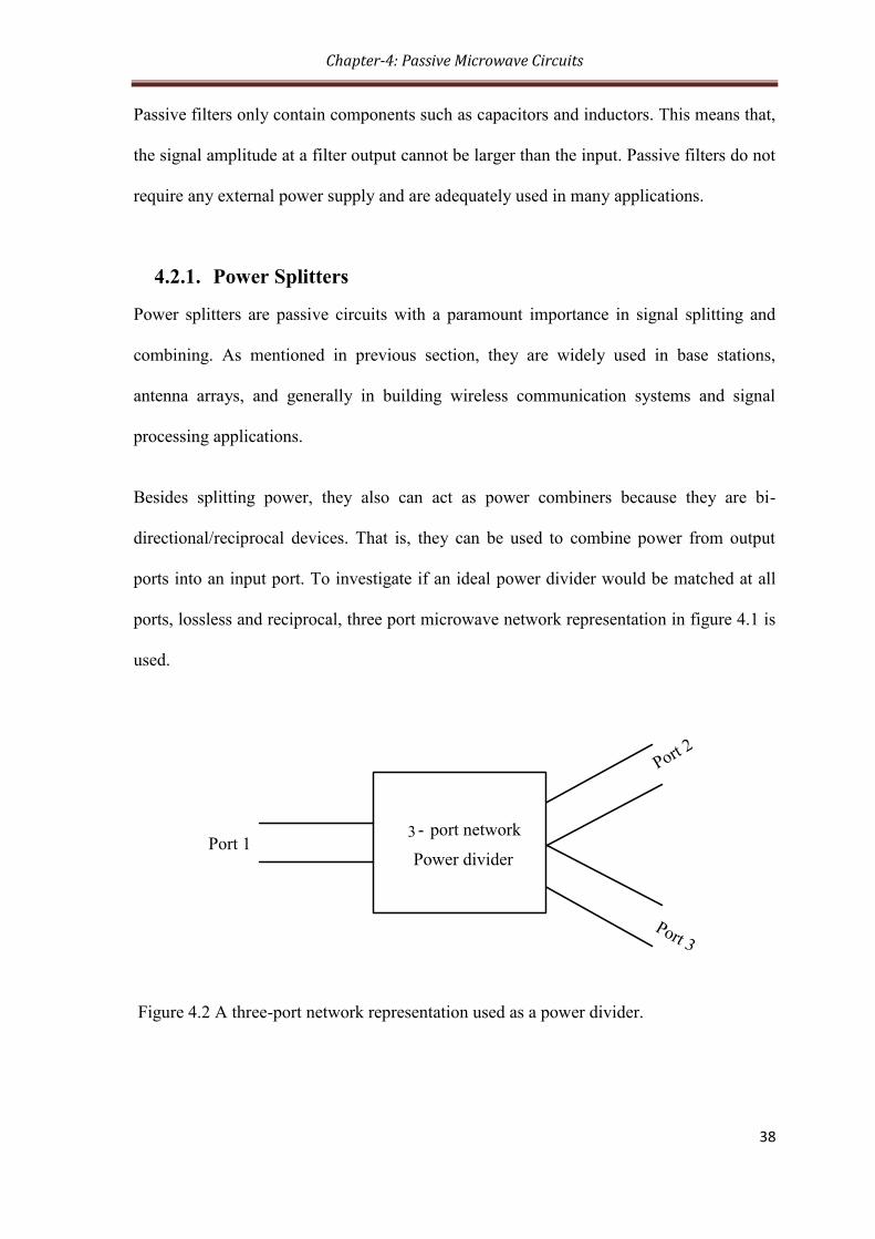
Besides splitting power, they also can act as power combiners because they are bi-
directional/reciprocal devices. That is, they can be used to combine power from output
ports into an input port. To investigate if an ideal power divider would be matched at all
ports, lossless and reciprocal, three port microwave network representation in figure 4.1 is
used.
3 - port network
Power divider
Port 2
Port 3
Port 1
Figure 4.2 A three-port network representation used as a power divider.
Chapter-4: Passive Microwave Circuits
39
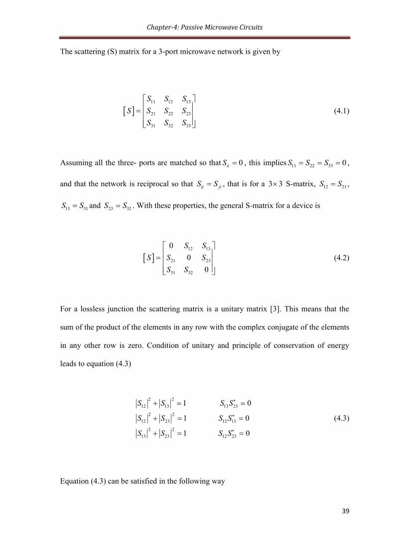
The scattering (S) matrix for a 3-port microwave network is given by
11 12 13
21 22 23
31 32 33
S S S
S S S S
S S S
(4.1)
Assuming all the three- ports are matched so that 0iiS , this implies 11 22 33 0S S S ,
and that the network is reciprocal so that ij jiS S , that is for a 3 3 S-matrix, 12 21S S ,
13 31S S and 23 32S S . With these properties, the general S-matrix for a device is
12 13
21 23
31 32
0
0
0
S S
S S S
S S
(4.2)
For a lossless junction the scattering matrix is a unitary matrix [3]. This means that the
sum of the product of the elements in any row with the complex conjugate of the elements
in any other row is zero. Condition of unitary and principle of conservation of energy
leads to equation (4.3)
2 2
12 13 13 23
2 2
12 23 12 13
2 2
13 23 12 23
1 0
1 0
1 0
S S S S
S S S S
S S S S
(4.3)
Equation (4.3) can be satisfied in the following way

Chapter-4: Passive Microwave Circuits
40
12 23 31 12 32 13
21 32 13 12 23 31
0 1
or
0 1
S S S S S S
S S S S S S
(4.4)
Equation (4.4) implies that for ij jiS S i j . Under this condition, the device must be
non reciprocal. The second column of equation (4.3) shows that at least two of the three
unique S-parameters must be zero. But if two of them were zero, then one of the equations
in the first column would be violated. From this we can conclude that it is impossible to
have a lossless, matched and reciprocal three port device.
4.2.1.1. Insertion and Reflection Losses
For a 3-port power splitter with tri-coupled resonators, the insertion loss parameters
between ports may be given by [8]
12 21
13 31
20log
20log
A
A
L S dB
L S dB
(4.5)
Where 12AL corresponds to the insertion loss between ports 1 and 2, and 13AL corresponds
to the insertion loss between ports 1 and 3 of figure 4.1. Similarly, the reflection loss at
port 1 may be defined as in [1] and [8]
2
11 1120log 10logRL S dB S dB (4.6)
The reflection loss is a measure of how well matched the network is. This is because it is a
measure of reflected signal attenuation.

Chapter-4: Passive Microwave Circuits
41
Applying conservation of energy formula to figure 4.3, we have
2 2 2
11 21 31 1S S S (4.7)
S13
12S
11S
Port 3
Port 2
Port 1
Represents resonator
Represents coupling
between resonators
Represents ports
Figure 4.3: Tri-resonator power splitter prototype
Assume that the power at the input port is divided between the two output ports 2 and 3
such that
2 2
21 31 , 1S S (4.8)
where is a constant.
Now substituting equation (4.8) into (4.7), we have
2 2
11 311 1 S S (4.9)
Now making use of equation (4.9) into equation (4.6) yields
2
3110log 1 1 RL S (4.10)

Chapter-4: Passive Microwave Circuits
42
Making 31S a subject gives
10
31
11 10
1RLS
(4.11)
and similarly, the transmission coefficient, 21S can be computed by substituting equation
(4.11) into equation (4.8), and this yields
10
21
1 10
1
RL
S
(4.12)
To obtain the insertion loss between input and output ports, equations (4.11) and (4.12)
can be used in (4.5) to yield
1
10 2
10
12
1
10 2
10
13
1 1020log = 10log 10log 1 10
1 1
1 10 120log = 10log 10log 1 10
1 1
R
R
R
R
L
L
A
L
L
A
L dB dB dB
L dB dB dB
(4.13)
And it follows that the insertion loss and return loss are related as in equation (4.13),
where the terms 10log 1
dB
and
110log
1dB
correspond to the maximum
values of 21 dBS and 31 dB
S , respectively [8].

Chapter-4: Passive Microwave Circuits
43
0
Ripple value
(dB)
-1 10 Frequency (Hz)
|S2
1| dB
10
log
1
dB
(a)
-20 -15 -10 -5 0 5 10 15 20
-33
-30
-27
-24
-21
-18
-15
-12
-9
-6
-3
0
Normalised frequency (rad/sec)
| S
21|(
dB
)
(b)
Figure 4.4: (a) Insertion Loss, S21 (dB) [8] and (b) 3-dB power splitter

Chapter-4: Passive Microwave Circuits
44
4.2.1.2. Power Splitter Polynomial
In the case of a two-port lossless filter network composed of series of N-inter-coupled
resonator filters, its reflection and transmission functions may be defined as a ratio of two
Nth
degree polynomials [30]
11 21( ) N N
N N
F s P sS s S s
E s E s (4.14)
where , and F P E are characteristic polynomials, and s j is the complex frequency
variable, and for Chebyshev filtering function, is a normalising constant for the
transmission coefficient to the equiripple level at 1 given by [30]
10
1
1.
10 1R
N
LN s
P s
F s
where RL is the return loss level in dB as defined in equation (4.10). It is assumed that
polynomials , and F s P s E s are normalised such that their highest degree
coefficients are unity.
For a 3-port power splitter consisting of tri-coupled resonators as described in figure 4.3,
equation (4.14) may be extended to describe the reflection and transmission functions as
follows [8]

Chapter-4: Passive Microwave Circuits
45
11 21 31
1 2
( ) F s P s P s
S s S s S sE s E s E s
(4.15)
and F s E s are the 3rd
order polynomials, and E s has its complex roots
corresponding to the filter pole positions. 1 and 2 are constants used to normalise
21 31( ) and ( )S s S s , respectively. E s can be constructed if , F s E s , 1 2 and are
known as in [8]. The expression for 1 2 and is shown in [30] as
1 210 10
1 1. .
10 1 10 1R RL L
s j s j
P s P s
F s F s
(4.16)
where is as in equation (4.8) in previous section.
1
2
3
Port 1
Port 2
Port 3
Figure 4.5 Topology of tri-resonator structure.
P s corresponds to the frequency locations of the transmission zeros. It is the
polynomial of order two because there are only two transmission zeros for the proposed
tri-resonator structure with 3-ports as shown in figure 4.5. This is mathematically proven

Chapter-4: Passive Microwave Circuits
46
and is presented in section 4.3.1.1. The solutions of F s describes the locations of
reflection zeros. In case of polynomial synthesis method, the reflection zeros can be
computed by using Cameron’s recursive technique as in [4], which will not be presented
in this thesis. A new approach is used to develop a clear synthesis procedure to design a
tri-coupled resonator power splitter consisting of only three resonators. To begin with, a
set of simple formulae to compute the coupling coefficients and external quality factors
are derived from reflection coefficient, 11S and transmission coefficients 21S and 31S . This
technique is discussed further in the next section.
4.3. Coupling matrix Method for Designing Filters
Coupling coefficients of inter-coupled resonator filters and external quality factors of the
input and output resonators are the basis for designing coupled resonator filters. Different
techniques of designing microwave filters such as network synthesis, polynomial and
coupling matrix synthesis method are presented in [2], [8], [11-13] and [17-18].
In this section practical filter design using normalised coupling matrix method will be
explored. The design procedure starts with developing mathematical expressions to
calculate the normalised coupling coefficients and the external quality factors using the
general equations of S-parameters in equation (3.35).

Chapter-4: Passive Microwave Circuits
47
4.3.1. Derivation of Reflection and Transmission zero locations for a
3x3 Normalised Coupling Matrix
The calculation of coupling parameters such as the normalised coupling coefficients and
the external quality factors is an important step in this new design procedure. To realise
the proposed tri-resonator structure shown in figure 4.6 analytically, a mathematical
expression will be developed using the general 3 3 normalised coupling matrix, A
analogous to the normalised impedance matrix for the asynchronously tuned resonators
shown in Chapter 3, equation 3.11. Thus, the normalised coupling matrix, A is given by
11 12 13
1
21 22 23
2
31 23 33
3
1
1
1
e
e
e
p jm jm jmq
A jm p jm jmq
jm jm p jmq
(4.17)
The general equation of S-parameters of a tri-coupled tri-resonator structure in terms of a
3 3 coupling matrix, A is given in Chapter 3 in equation (3.35) and is presented here
again as
1
21 21
1 2
1
31 31
1 3
1
11 111
12
12
21
e e
e e
e
S Aq q
S Aq q
S Aq
(4.18)

Chapter-4: Passive Microwave Circuits
48
The variables 1eq , 2eq and 3eq are the external quality factors, p j is the complex
frequency variable, U is the n n identity matrix and m is the normalised coupling
matrix.
The inverse of a normalised coupling matrix in equation (4.18) can be described in terms
of the adjugate and determinant of matrix A as follows [12]
1
, det 0det
adj AA A
A
(4.19)
where adj A is the adjugate of a square matrix A , and det A is its determinant.
Noting that the adjugate of a matrix is the transpose of a matrix of cofactors created from a
matrix, A . Thus, using this definition, equation (4.19) can be re-defined more precisely
as
1 1
1 , det 0
det
n
n
cof AA A
A
(4.20)
Where 1
1nA
is the ,1n element value of the inverse matrix, A , and 1ncof A is the
1,n element of the cofactor matrix, A for 1, 2n and 3.
Making use of equation (4.20) and substituting into equation (4.18) yields
12 13
21 31
1 2 1 3
11
11
1
2 2. .
det det
2 1 .
det
e e e e
e
cof A cof AS S
A Aq q q q
cof AS
q A
(4.21)
Chapter-4: Passive Microwave Circuits
49
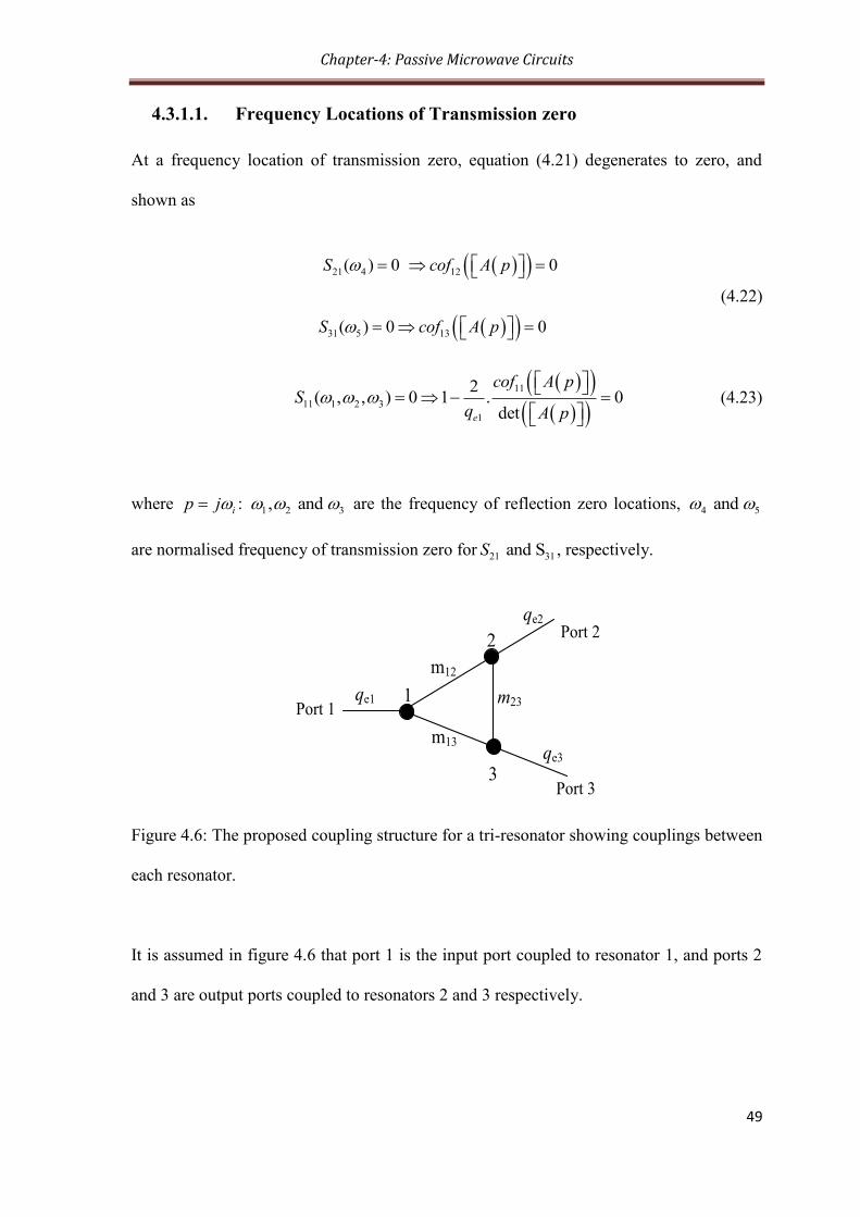
4.3.1.1. Frequency Locations of Transmission zero
At a frequency location of transmission zero, equation (4.21) degenerates to zero, and
shown as
21 4 12
31 5 13
( ) 0 0
( ) 0 0
S cof A p
S cof A p
(4.22)
11
11 1 2 3
1
2( , , ) 0 1 . 0
dete
cof A pS
q A p
(4.23)
where ip j : 1 2 3, and are the frequency of reflection zero locations, 4 5 and
are normalised frequency of transmission zero for 21 31 and SS , respectively.
m12
m13
m231
2
3
Port 1
Port 2
Port 3
qe1
qe2
qe3
Figure 4.6: The proposed coupling structure for a tri-resonator showing couplings between
each resonator.
It is assumed in figure 4.6 that port 1 is the input port coupled to resonator 1, and ports 2
and 3 are output ports coupled to resonators 2 and 3 respectively.

Chapter-4: Passive Microwave Circuits
50
From equation (4.22), the
12cof A p and 13cof A p can be computed and
shown as
12 12 33 13 23
43
13 12 23 13 22
52
1 c = 0
1 c ( ( )) 0
e
e
of A p jm jm p m mp jq
of A p m m jm jm pp jq
(4.24)
The detailed calculations are given in Appendix B. Rearranging equation (4.24) for the
transmission zero locations for 21 31 and SS yields
13 234 33
12 3
12 235 22
13 2
1
1
e
e
m mm j
m q
m mm j
m q
(4.25)
For synchronously tuned filter, where 11 22 33 0m m m , equation (4.25) will further
reduce to
13 234
12 3
12 235
13 2
1
1
e
e
m mj
m q
m mj
m q
(4.26)
From equation (4.26) it may readily be seen that there are two transmissions zero locations
for the proposed structure shown in figure 4.6 with all resonators are coupled to one
another.

Chapter-4: Passive Microwave Circuits
51
4.3.1.2. Frequency Locations of Reflection zeros
Similarly, we will continue to find 11cof A p and det A p as a function of
normalised coupling coefficients and external quality factors. Thus, from equation (4.23),
the 11cof A p is
2
11 22 33
3 2
2 332222 33 23
2 3 3 2
1 1( )
1 ( )
e e
e e e e
cof A p p jm jm pq q
mmm m m j j
q q q q
(4.27)
while the det A p
is
211 22 1111 22 33 11 22 11 33 11
3 3
211 33 22 3311 11 2211 23
2 2 2 3 1 1
2
33 3322
1 3 1 1 1 3 1 2 1 2 1 2 3
2
23
22 3
1
det
1
e e
e e e e e e
e e e e e e e e e e e e e
e
m m jm pA p jm m m m m p m m p jm p
q q
m m m mjm p jm jm pjm m
q q q q q q
jm p jmjm p p p
q q q q q q q q q q q q q
mm m
q
22 3 3322
3 22 33
3 3 2
222 2 2 12
23 12 33 12
2 2 3 3
22 2 13
12 13 23 13 22 13
2
( ) ( ) ( )
( )2 ( ) ( )
e e e
e e e e
e
jm pjm p pp jm p jm p p
q q q
mp pp m j m m m p
q q q q
mj m m m j m m m p
q
(4.28)
The detailed derivation of 11cof A p and det A p are shown in Appendix B.
Substituting equations (4.27) and (4.28) into equation (4.23), yields

Chapter-4: Passive Microwave Circuits
52
3 2
11 1 2 3 11 22 33
3 2 1
2 2 2
11 22 11 33 22 33 23 12 13
1 2 1 3 2 3
1 1 1( , , )
( )
1 1 1
e e e
e e e e e e
S j j j p j m m m pq q q
m m m m m m m m m p
pq q q q q q
22 33 11 33 11 22
1 2 3
2 2 2
22 33 23 13 11 33 12 11 22
1 2 3 1 2 3
11
2
1
e e e
e e e e e e
e e
m m m m m mj p
q q q
m m m m m m m m m
q q q q q q
mj
q q
2 2332211 23 22 13
3 1 3 1 2
2
33 12 13 12 23 11 22 33
2 0
e e e e
mmm m m m
q q q q
j m m m m m m m m
(4.29)
Equation (4.29) is the general expression to compute reflection zero locations for
asynchronously tuned tri-coupled tri-resonator filter structure shown in figure (4.6). It is
also applicable for synchronously tuned tri-resonator filters with the assumption that no
self couplings are considered, that is for 11 22 33 0m m m . It is worth mentioning that
there are 12 unknown parameters in equation (4.29). These are 6 normalised coupling
coefficients ( 11 12 13 22 23 33, , , , , m m m m m m ), 3 scaled external quality factors
( 1 2 3, and e e eq q q ) and 3 reflection zero locations ( 1 2 3, and p p p ).

Chapter-4: Passive Microwave Circuits
53
A complete solution will be sought to fully realise the proposed tri-coupled tri-resonator
structure. To find these analytically, mathematical manipulations of equation (4.29) along
with some assumptions are further explored and presented in chapter 5 in detail.
By defining
11 22 33
3 2 1
1 1 1
e e e
a j m m mq q q
(4.30)
2
11 22 11 33 22 33 23
2 2
12 13
1 2 1 3 2 3
22 33 11 33 11 22
1 2 3
1 1 1 ( )
e e e e e e
e e e
b m m m m m m m
m mq q q q q q
m m m m m mj
q q q
(4.31)
and
2 2 2
22 33 23 13 11 33 12 11 22
1 2 3 1 2 3
2 23311 2211 23 22 13
2 3 1 3 1 2
2
33 12 13 12 23 11 22 33
1
2
e e e e e e
e e e e e e
m m m m m m m m mc
q q q q q q
mm mj m m m m
q q q q q q
j m m m m m m m m
(4.32)
equation (4.29) can be rewritten

Chapter-4: Passive Microwave Circuits
54
3 2
11 ( ) 0S p f p p ap bp c (4.33)
The solution to this equation is what we require. This is given in Appendix A. It is clear
that this is a very complex to solve for the zeros of this function which is shown in
Appendix A. To simplify the problem, the cubic equation can be written in terms of the
three solutions as
3 2
11 1 1 1 1
3 2
11 2 2 2 2
3 2
11 3 3 3 3
0
0
0
S p p ap bp c
S p p ap bp c
S p p ap bp c
(4.34)
Where 1 2,p p and 3p are the zeros of (4.33) and the frequency locations of the reflection
zeros.
Now we can guess the frequency locations of the reflection zeros in order to avoid the
complexity. 1 1p j , 2 2p j and 3 3p j , where 1 1 , 2 0 and 3 1 are put a
first step in the process of trying to simplify the problem. There are of course no reasons
why these should be solutions of (4.33), but we will continue to investigate. Thus,
mathematical analysis in chapter 5 is based on these values of reflection zeros.
It should be pointed out that for the examples presented in this thesis, the responses of the
tri-resonator structures are not conventionally normalised, i.e., the cut off frequency is not
±1 rad/sec. However, these responses can be easily transformed (or normalised) simply by

Chapter-4: Passive Microwave Circuits
55
multiplying a constant with all the coupling coefficients of the coupling matrices to
renormalize the bandpass edge to ±1 rad/sec. This will of course make 1 1 and 3 1 .
Using these values in (4.33) will give us
11 1,2,3 0S p
11 ,0, 2 3S j j a c (4.35)
Substituting for a and c in (4.34) gives the following expression
11 22 33
3 2 1
2 2 2
22 33 23 13 11 33 12 11 22
1 2 3 1 2 3
2 23311 2211 23 22 13 33
2 3 1 3 1 2
1 1 1
1 3
3
11
e e e
e e e e e e
e e e e e e
S -j,0, j = -2 j m m m +q q q
m m m m m m m m m
q q q q q q
mm mj m m m m m m
q q q q q q
2
12 13 12 23 11 22 332 0m m m m m m
(4.36)
From equation (4.25)
12
23 33 4
13 3
1
e
mm m j
m q
(4.37)
or

Chapter-4: Passive Microwave Circuits
56
13
23 22 5
12 2
1
e
mm m j
m q
(4.38)
Note that equations (4.37) and (4.38) are equal. The back substitution of these equations
into equation (4.33) will further simplify the expression. We have now setup the solution
and manipulations of this will be seen in the next chapter. In the process of designing 3-dB
tri-resonator power splitter, the analysis and application of equation (4.33) or (4.30) are
also presented in the next chapter.

Chapter-5: Microwave Tri-resonator Filter Structures
57
Chapter 5
Microwave Tri-resonator Filter Structure
5.1. 3-dB Tri-resonator Power Splitter Coupling Matrix
Synthesis
The lowpass prototype design of a 3-dB power splitter is presented in this section. The
power splitter frequency response is assumed to be symmetrical. For a symmetrical
frequency response an equal power division between output ports 2 and 3 is considered.
This is illustrated analytically, and the design parameters for a 3-dB tri-resonator power
splitter are calculated. For the practical design, the following assumptions are made and
used throughout a mathematical analysis to calculate the normalised coupling coefficients
and external quality factors for splitter design.
5.1.1. Design procedure for Power Splitter with no Coupling between
Resonators 2 and 3
Consider the following assumptions and the topology shown in figure 5.1.
'
11 22 33 12 13 23 2 30, , 0, e e em m m m m m q q q (5.1)
m12
m12
1
2
3
Port 1
Port 2
Port 3
qe1
'
eq
'
eq
23 0m
Figure 5.1: 3-dB power divider topology with output ports 2 and 3 are uncoupled

Chapter-5: Microwave Tri-resonator Filter Structures
58
These assumptions will transform the topology proposed for tri-coupled tri-resonator
structure shown in chapter 4, figure 4.6 into tri-resonator power splitter structure as shown
in figure 5.1.
Based on the assumptions, there are only two possible reflection zeros for the topology
shown in figure 5.1. The same values of frequency locations of reflection zeros used in
equation (4.34) can also be assumed here but using 2 2 ,p j where 2 0 into equation
(4.34) gives non-zero value. This value is said to be the peak value of the return loss, r of
the response.
Thus recalling equation (4.32), and using 1 2 3, 0 and p j p p j , into it yields
11 1 0S p j j a jb c (5.2)
11 2 0S p c r (5.3)
11 3 0S p j j a jb c (5.4)
where 2010RL
r
in linear form, and RL in dB-scale and should be in the range of
0 RL .
Taking the summation of equation (5.2) and (5.4) gives
0a c
(5.5)
By using the assumptions in equation (5.1) into equation (4.30-4.32) in chapter 4, the
parameters a and c can be shown as
'
1
1 2
e e
aq q
, 2
12
' ' 2
1
2 1
e e e
mc
q q q (5.6)
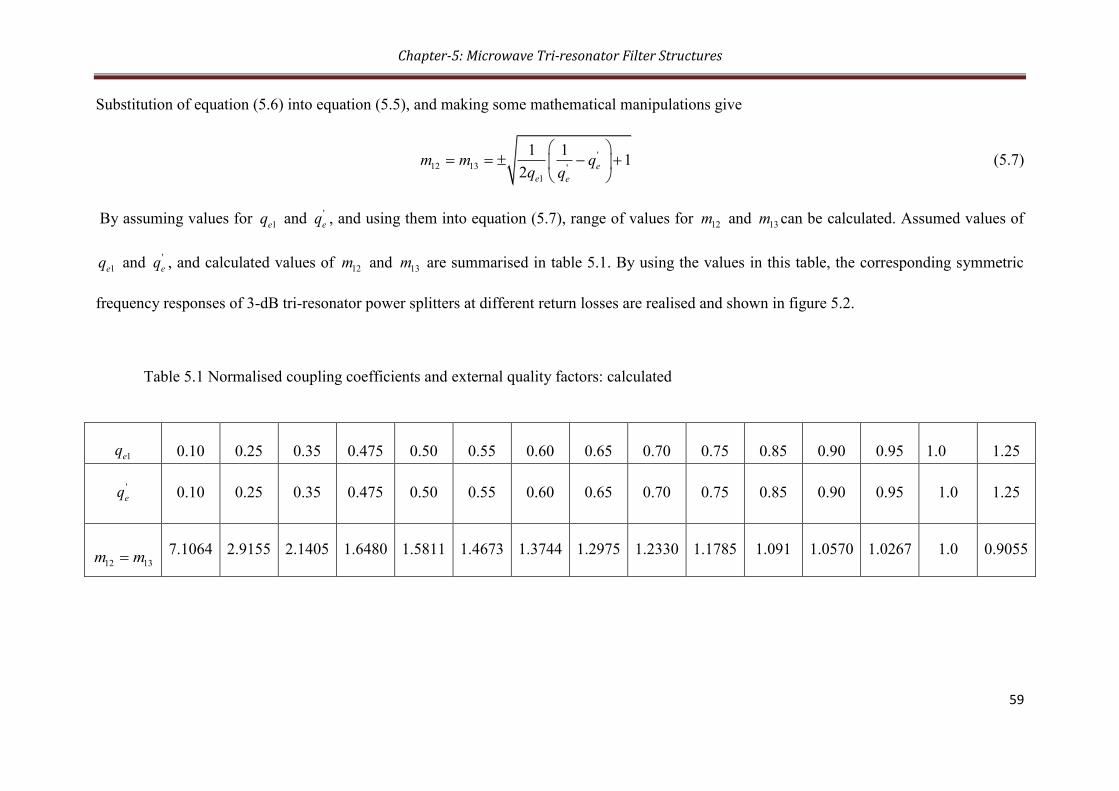
Chapter-5: Microwave Tri-resonator Filter Structures
59
Substitution of equation (5.6) into equation (5.5), and making some mathematical manipulations give
'
12 13 '
1
1 11
2e
e e
m m qq q
(5.7)
By assuming values for 1eq and '
eq , and using them into equation (5.7), range of values for 12m and 13m can be calculated. Assumed values of
1eq and
'
eq , and calculated values of 12m and 13m are summarised in table 5.1. By using the values in this table, the corresponding symmetric
frequency responses of 3-dB tri-resonator power splitters at different return losses are realised and shown in figure 5.2.
Table 5.1 Normalised coupling coefficients and external quality factors: calculated
1eq 0.10 0.25 0.35 0.475 0.50 0.55 0.60 0.65 0.70 0.75 0.85 0.90 0.95 1.0 1.25
'
eq 0.10 0.25 0.35 0.475 0.50 0.55 0.60 0.65 0.70 0.75 0.85 0.90 0.95 1.0 1.25
12 13m m 7.1064 2.9155 2.1405 1.6480 1.5811 1.4673 1.3744 1.2975 1.2330 1.1785 1.091 1.0570 1.0267 1.0 0.9055

Chapter-5: Microwave Tri-resonator Filter Structures
60
-20 -15 -10 -5 0 5 10 15 20-80
-70
-60
-50
-40
-30
-20
-10
0
Normalised frequency (rad/sec)
|S11| d
B,| S
21| d
B,|S 3
1| d
B
S11
1
S21
1
S31
1
S11
2
S21
2
S31
2
S11
3
S21
3
S31
3
S11
4
S21
4
S31
4
S11
5
S21
5
S31
5
S11
6
S21
6
S31
6
S11
7
S217
S317
S118
S218
S318
S119
S219
S319
S1110
S2110
S3110
S1111
S2111
S3111
S1112
S2112
S3112
S11
13
S21
13
S31
13
S11
14
S21
14
S31
14
S11
17
S21
17
S31
17
Figure 5.2 Frequency responses of a 3-dB tri-resonator power splitter for the topology
shown in figure 5.1.
Figure 5.2 demonstrates various splitter responses at reflection zeros of j with different
reflection losses. The reflection zero locations have been forced to be j as it has been
explained in the mathematical derivation to calculate the normalised coupling coefficients
and external quality factors in chapter 4, section 4.3.1.2.
By referring to table 5.1, one can design a 3-dB tri-resonator power splitter with a goal of
specific return loss (RL). For instance, if we want to realise a symmetric frequency
response of 3-dB tri-resonator power splitter at 20 dB return loss, the normalised coupling
coefficients, 12 13 and m m , and external quality factors, '
1 and e eq q can be read from table

Chapter-5: Microwave Tri-resonator Filter Structures
61
5.1 as '
1 e 12 13=q =0.475 and = =1.6480eq m m .The frequency response for this particular
values is given in figure 5.3.
-15 -10 -5 0 5 10 15-60
-50
-40
-30
-20
-10
0
|S1
1| d
B,|S
21
| d
B,|S
31
| d
B
Normalised frequency (rad/sec
S11
S21
=S31
Figure 5.3 A 3-dB power splitter response at -20 dB return loss
To investigate the return loss, r equations (5.2-5.4) are further simultaneously computed
as follows:
Subtracting equation (5.2) with equation (5.3) yields
j a jb r (5.8)
and subtracting equation (5.3) from equation (5.4) gives
j a jb r (5.9)
Chapter-5: Microwave Tri-resonator Filter Structures
62
Solving equation (5.8) and (5.9) simultaneously gives 1b , and using this into (5.8)
yields a r . Also it is clear from equation (5.3) that c r . Thus , and a r c are related as
a r c (5.10)
Recalling the definitions of a , b and c in equations (4.28-4.30), and making use of
equation (5.1) into them may give the following expressions for a , b and c as
'
1
1 2
e e
aq q
, 2
12
' ' 2
1
2 1
e e e
mc
q q q (5.11)
2
12 ' ' 2
1
2 12
e e e
b mq q q
(5.12)
Substitution of equation (5.11) into (5.10) gives
'
2
12 '
1 1
12 2e
e
qm r
q q q
2
12 '
1
12
e
r mq q
(5.13)
Using 1b in equation (5.12), and making 2
12m a subject yields
2
12 ' ' 2
1
1 2 11
2e e e
mq q q
(5.14)
Substitution of equation (5.14) into equation (5.13) gives the return loss as a function of
normalised external quality factors. This is shown as

Chapter-5: Microwave Tri-resonator Filter Structures
63
' 2 ' '
1
1 1 1 1
ee e e
rqq q q
(5.15)
It should be noted that the return loss lies in the range of 0 1r for passive circuit or in
the range of negative infinity to zero in the dB-scale; i.e., 0RL dB.
The graph of return loss versus the external quality factor, 2eq and 3eq at the output ports
2 and 3 respectively is presented in figure 5.4. For the sake of clarity, the relationship
between 1eq and '
eq is given by '
1e eq q where 0.15 1 is considered and shown as
a non-parabolic part of figure 5.4 for the range of 0 1r . However, for 1.25 6.25 ,
the return loss responses are parabolic as elaborated in figure 5.4.
0 0.1 0.2 0.3 0.4 0.5 0.6 0.7 0.8 0.9 10
1
2
3
4
5
6
7
8
9
10
Return loss (r)
Ex
tern
al
qu
ali
ty f
acto
r, q e2=
q e3=
q' e
qe1
=0.15q'e
qe1
=0.35q'e
qe1
=0.55q'e
qe1
=0.75q'e
qe1
=0.85q'e
qe1
=q'e
qe1
=1.25q'e
qe1
=1.75q'e
qe1
=2.25q'e
qe1
=2.75q'e
qe1
=3q'e
qe1
=3.25q'e
qe1
=3.75q'e
qe1
=4.25q'e
qe1
=4.75q'e
qe1
=5.25q'e
qe1
=5.75q'e
qe1
=6.25q'e
Figure 5.4 External quality factors versus, r , for '
1e eq q where 0.15 6.25

Chapter-5: Microwave Tri-resonator Filter Structures
64
From figure 5.4, it can be seen that an infinite number of external quality factors at the
output ports can be collected at a desired ripple value. For a specific return loss value, two
different values of '
eq can be read. This is because of the parabolic nature of the graphs in
figure 5.4 for the case when1.25 6.25 is considered. For instance, for the case
'
1 1.25e eq q in figure 5.4, at a particular value of r , say 0.25r , '
eq has two values,
and may be read as 0.49 and 4.0. At these two values of '
eq , there are two corresponding
values of normalised coupling coefficients, 12m where 12 13m m in figure 5.5, and this is
consistent with equation (5.7); i.e., 12 13m m can be negative or positive values.
Using the appropriate values of '
eq from figure 5.4 at a particular return loss, r , and the
corresponding values of coupling coefficients from figure 5.5, a 3-dB power splitter
parameters can be determined. Figure 5.5 shows the external quality factors versus the
positive coupling coefficients. For the negative coupling coefficients, 12 13m m versus
external quality factor can be drawn simply by taking the mirror image of figure 5.5, and
hence, the negative values of 12 13m m can be extracted. These illustrate that 12m and 13m
hold negative or positive values as discussed and has also been analytically proven and
shown in equation (5.7).
It should be noted that the mirror image of figure 5.5 which gives rise to the negative
values of coupling coefficients does not mean that the negative values of coupling
coefficients give rise to an image frequency response of the splitter. Instead, the positive
and negative values of 12m and 13m give same symmetric frequency response of 3-dB tri-
resonator power splitters and this is presented in the next section as examples.

Chapter-5: Microwave Tri-resonator Filter Structures
65
Figure 5.5 The relationship between normalised coupling coefficients and external quality
factors for 12 13 0m m in log scale.
The response in figure 5.5 describes the degree of freedom in reading multiple values of
12m and 13m for a corresponding values of '
eq directly from it. Besides this, we can have
3-dB tri-resonator power splitter of identical responses with diferent values of coupling
coefficients and external qaulity factors. These responses are shown in the design
examples 1 and 2 in the next section. It can be noted from figure 5.5 that; at a point 1, 1 ,
the responses of the coupling coefficients, m intersect.

Chapter-5: Microwave Tri-resonator Filter Structures
66
The design procedure can be summarised in 4 steps as follows:
1. Determine the return loss , r from figure 5.4
2. Read the values of external quality factors from figure 5.4 at input port 1 and
output ports 2 and 3
3. For the corresponding values of '
eq in figure 5.4, read the corresponding values of
coupling coefficients from figure 5.5
4. Determine the response of the power splitter topology shown in figure 5.1
5.1.2 Coupling Matrix Power Divider Examples
Using the design procedure outlined the following 3-dB tri-resonator power splitters are
designed and presented. The normalised coupling matrix and external quality factors
illustrated in examples 1 and 2 are extracted from figure 5.5. These are some of the values
we are interested in for the design purpose to get better responses. It is also interesting to
note that the coupling matrices and external quality factors demonstrated in design
examples 1 and 2 can also be calculated using equation 5.7, and found to be consistent
with the values from the graph of coupling coefficients versus '
eq -factor as expected.
The intention in the design examples 1 and 2 is to show how two different coupling
matrices and external quality factors can be used to design same tri-resonator power
splitter responses.
Design Example 1:
In this example, two different normalised coupling matrices and external quality factors
are used to give exactly the same response with a return loss of 20.33 dB as shown in

Chapter-5: Microwave Tri-resonator Filter Structures
67
figures 5.6 and 5.6. This is possible as the graph in figure 5.4 is parabolic and two values
of normalised external quality factors for a single value of return loss can be obtained.
'
1
0 1.6875 1.6875
= 1.6875 0 0
1.6875 0 0
0.4615=
a
e e
m
q q
-15 -14 -13 -12 -11 -10 -9 -8 -7 -6 -5 -4 -3 -2 -1 0 1 2 3 4 5 6 7 8 9 10 11 12 13 14 1515-60
-50
-40
-30
-20
-10
0
Inse
rtio
n a
nd R
efl
ecti
on L
oss
es
(dB
)
Normalised frequency (rad/sec)
S11
S21
=S31
(b)
Figure 5.6 (a) Normalised coupling matrix and external quality factors and (b) A 3-dB tri-
resonator power splitter with the bandpass edge of ±1.45 rad/s.

Chapter-5: Microwave Tri-resonator Filter Structures
68
'
1
0 1.6799 1.6799
= 1.6799 0 0 , = 0.4640
1.6799 0 0
e em q q
(a)
-15 -14 -13 -12 -11 -10 -9 -8 -7 -6 -5 -4 -3 -2 -1 0 1 2 3 4 5 6 7 8 9 10 11 12 13 14 1515-60
-50
-40
-30
-20
-10
0
Inse
rtio
n a
nd R
efl
ecti
on L
oss
es
(dB
)
Normalised frequency (rad/sec)
S11
S21
=S31
(b)
Figure 5.7 (a) Normalised coupling matrix and external quality factors and (b) A 3-dB tri-
resonator power splitter with the bandpass edge of ±1.45 rad/s.
The tri-resonator power splitter responses shown in figure 5.6 and 5.7 are the same as
expected except that the normalised coupling matrices and external quality factors
obtained are different. The two graphs are therefore, evident that exactly the same
responses of a tri-resonator power splitter can be designed using two different normalised
coupling matrices and external quality factors as discussed above in this section. The
power splitter responses in figure 5.6 and 5.7 have the same bandwidths. This is the case

Chapter-5: Microwave Tri-resonator Filter Structures
69
as their bandpass edges are equal and is ±1.45 rad/sec. Thus, both splitters have bandwidth
of 2.9 rad/sec.
Design Example 2:
In a similar way to design example 1, there are two distinct coupling matrices and external
quality factors that yield same 3-dB tri-resonator power splitter with a return loss goal of
21.75 dB as shown in figures 5.8 and 5.9. These responses are obtained by using the two
different coupling coefficients and external quality factors, and compared with each other.
'
1
0 1.8191 1.8191
= 1.8191 0 0 , 0.4219=
1.8191 0 0
e em q q
(a)
-15 -14 -13 -12 -11 -10 -9 -8 -7 -6 -5 -4 -3 -2 -1 0 1 2 3 4 5 6 7 8 9 10 11 12 13 14 1515-70
-60
-50
-40
-30
-20
-10
0
Inse
rtio
n a
nd R
efle
ctio
n L
oss
es (
dB
)
Normalised frequency (rad/sec)
S11
S21
=S31
(b)
Figure 5.8 (a) Normalised coupling matrix and external quality factors and (b) Response
of a 3-dB tri-resonator power splitter with the bandpass edge of ±1.5rad/s.

Chapter-5: Microwave Tri-resonator Filter Structures
70
'
1
1.832 1.832
0
1.832 0 0
1.832 0 0
0.4184=
e e
m
q q
(a)
-15 -14 -13 -12 -11 -10 -9 -8 -7 -6 -5 -4 -3 -2 -1 0 1 2 3 4 5 6 7 8 9 10 11 12 13 14 1515-70
-60
-50
-40
-30
-20
-10
0
Inse
rtio
n a
nd R
efl
ecti
on L
oss
es
(dB
)
Normalised frequency (rad/sec)
S11
S21
=S31
(b)
Figure 5.9 (a) Normalised coupling matrix and external quality factors and (b)
Response of a 3-dB tri-resonator power splitter with the bandpass edge of ±1.5
rad/sec.

Chapter-5: Microwave Tri-resonator Filter Structures
71
It can be seen from example 1 and 2 that the same 3-dB tri-resonator power splitter of
identical response has been designed with different normalised coupling coefficients and
external quality factors as explained earlier in this section.
The bandwidth of the power splitter responses shown in figure 5.8 and 5.9 are the same as
they have the same bandpass edge, i.e., ±1.5 rad/sec.
From the design examples, it can be concluded that the range of values of coupling matrix
and external quality factors can be calculated to design power splitters of identical
responses.
In both design examples, the 3-dB tri-resonator power splitters having only one pair of
transmission zeros have been designed.
5.2. Trisection Filter
A trisection filters comprise three couplings between three sequentially-numbered
resonator filters. The first and third of which may be source or load terminals or it might
be embedded within the coupling matrix of a higher-degree network [1]. As shown in
figure 4.14, trisections are able to realize one transmission zero, and this is analytically
proved in the next section. Figure 5.14 shows topology of trisection filter with the cross
coupling between resonators 1 and 3, where it is assumed that the input and output ports
are coupled to resonators 1 and 3 respectively. The cross coupling between resonators
along with other couplings gives controllable transmission zero. We will see this shortly in
this section when we work on the mathematical analysis of designing a trisection filter.

Chapter-5: Microwave Tri-resonator Filter Structures
72
The placement of transmission zero is determined by the polarity of the cross coupling
between resonator 1 and 3. The topology of the coupling arrangement is shown in figure
5.10.
Port 1 Port 2
m13
m12 m23
3 21
Source/load Resonator
Figure 5.10 A tri-section filter showing the coupling between each resonator.
The direct and cross coupling phenomenon shown in figure 5.10 may be illustrated as
follows:
12m represents the direct coupling between resonators 1 and 2, 13m describes the cross
coupling between resonators 1 and 3 and 23m stands for the main coupling between
resonators 2 and 3.
The ability to realise just one transmission zero at finite frequency, makes the trisection
filter very useful in synthesising filters with asymmetric characteristics. Trisection filters
can exist either as a stand-alone within the network or multiply as a cascade. We will
investigate a trisection filter with the type of topology shown in figure 5.10. We will not
go further for multiple trisection filters which exist as cascaded within a network.

Chapter-5: Microwave Tri-resonator Filter Structures
73
5.2.1. Analysis
Putting 2eq to infinity at port two of a three port tri-section filters topology described in
figure 4.6 gives tri-coupled trisection filter structure shown in figure 5.10. This will
transform the 3-port tri-resonator structure into two ports (input and output ports).
For a two port network the reflection and transmission S-parameters are given by
1 11
1111
1 1
1 13
2131
1 3 1 3
2 21 1 .
det
1 22 .
det
e e
e e e e
cof AS A
q q A
cof AS A
Aq q q q
(5.16)
The transmission zero location may be found from equation (4.26). This may be shown as
12 23
22 2
13
for e
m mm q
m (5.17)
where is the transmission zero.
A trisection filter requires the resonators to be asynchronously tuned to give an
asymmetric filter frequency response [1]. Thus the resonating frequency for each resonator
may be different. It will have an attenuation pole at one side of the passband.

Chapter-5: Microwave Tri-resonator Filter Structures
74
To keep the physical configuration of the filter symmetrical even though the frequency
response is asymmetric, the following assumptions are made [1]
''
12 23 1 3 01 03, , e e em m q q q (5.18)
where 01 and 03 are the angular frequencies of resonator 1 and 3, respectively.
Using these assumptions and 2eq in equation (4.32) yields
11 11 22 33 22 33 11 22''
2 22212 11 33 13 22 13 11 22 33'' 2
3,0, 2
3 2 0
e
e
S j j j m m m m m m mq
mj m m m m m m m m m
q
(5.19)
Equation (5.17) may be re-arranged for 12m and shown by
2
12 13 22m m m (5.20)
Substitution of equation (5.20) into (5.19) gives the general expression as the function of
transmission zero location, at reflection zeros, ,0 and j j , and presented as
11 11 22 33 22 33 11 22''
2 22
22 13 11 22 33 '' 2
13 22 11 33 13
3,0, 2
3
3 2 0
e
e
S j j j m m m m m m mq
mj m m m m m
q
j m m m m m
(5.21)

Chapter-5: Microwave Tri-resonator Filter Structures
75
This calculation can be taken one stage forward if 11 33m m is assumed, and substituted
into equation (5.21). Thus, shown as
11 22 13 22 11 13
2 2 2222 13 11 22 '' 2
2 2 3 2
3 3 0
e
j m m j m m m m
mj m m m m j
q
(5.22)
To have same return loss level (or equal ripple) design, the following mathematical
manipulations are carried out:
The first derivative of equation (4.33) is set to zero, and the peak frequency values of 11S
in the passband may be computed as
3 2
11
2 2
0 0
23 2 0
3 3
d dS p p ap bp c
dp dp
a bp ap b p p
where , and a b c are coefficients of the cubic function as defined in equations (4.30-
4.32).
The roots of p can be found by completing the square method, and given as
2 3
3
a a bp
(5.23)
Two peak frequency values can be picked up from equation (5.21), and these are given as

Chapter-5: Microwave Tri-resonator Filter Structures
76
2 2
1 2
3 3 s
3 3r r
a a b a a bs j j
The locations of these two peak frequency at which the return loss response will have
equiripple values are demonstrated in figure 5.11.
For 2 12 23 11 33, and q m m m m , the parameters , a b and c
are given as
11 22
2 2 2
11 22 11 12 13 '' 2
2 2
13 22 11 13 22 13 11 '' 2
2
22 2 ( )
12
a j m m
b m m m m mq
c j m m m m m m mq
Now evaluating 11S at 1rs and r2s gives return loss value r , where 2010
RL
r
for
0 dBRL . This is shown as
1 2 1 2, 0, 0r r r rS s r S s r S s r S s r
20 201 210 0, 10 0
RL RL
r rS s S s
(5.24)
Or equation (5.23) can be generalised as
2
2011
1
10 0sri
RL
i
S
(5.25)
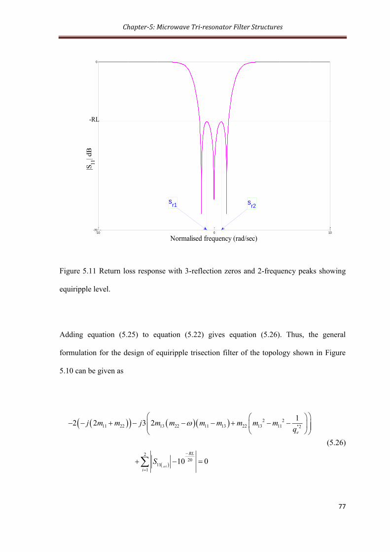
Chapter-5: Microwave Tri-resonator Filter Structures
77
-10 0 10-70
0
Normalised frequency (rad/sec)
|S11| d
B
sr1 s
r2
-RL
Figure 5.11 Return loss response with 3-reflection zeros and 2-frequency peaks showing
equiripple level.
Adding equation (5.25) to equation (5.22) gives equation (5.26). Thus, the general
formulation for the design of equiripple trisection filter of the topology shown in Figure
5.10 can be given as
2 2
11 22 13 22 11 13 22 13 11 ''2
2
2011
1
12 2 3 2
10 0sri
e
RL
i
j m m j m m m m m m mq
S
(5.26)

Chapter-5: Microwave Tri-resonator Filter Structures
78
It is evident from the mathematical function in equation (5.26) that there are only 3
unknown normalised coupling coefficients, 11 22 13, and m m m , and an external quality
factor, ''
eq that need to be evaluated. That means, only 4 unknown variables,
''
11 13 22, , , and em m m q appeared in equation (5.26). The frequency location of transmission
zero, in equation (5.26) can be controlled and set to a value. We have successfully
reduced the 12 full solutions in equation (4.29) to 4 solutions through the mathematical
analysis described. This has a benefit of reducing the computation time during the
optimisation process. By optimisation, we meant minimising the function expression in
equation (5.26). To do this, optimisation process has to be implemented to generate
optimal values of the normalised coupling coefficients and external quality factors so that
the given function in equation (5.26) is minimised. This is explained in the next section.
An optimisation algorithm used and the iteration process carried out to design trisection
filter is also presented in the next section.
5.2.2. Optimisation
Different techniques of optimisation have been utilized to synthesise coupled resonator
filters. One of these techniques is based on optimisation of the normalised coupling
coefficients in a normalised coupling matrix. The main advantage of coupling matrix
optimisation technique is that it requires considerably less computational time than full
scale EM simulations to complete the synthesis [8]. In this work, to realise a trisection
filter, coupling matrix optimisation technique is used to obtain the coupling coefficients
and the external quality factors in equation (5.26). Thus, equation (5.26) can be used as a
cost function when using optimisation. The cost function in equation (5.26) is provided as

Chapter-5: Microwave Tri-resonator Filter Structures
79
a function of 4 control variables (normalised coupling coefficients and external quality
factors).
We have used an optimisation algorithm that uses unconstrained control variables to un-
bound the search space so as to make a direct search starting from the initial guess. This is
known as local optimisation algorithms. Local optimisation algorithms strongly depend on
the initial values of the control parameters. The initial guess should be given as an input to
the algorithm that seeks a local minimum within the local neighbourhood of the initial
guess.
Initial values of control variables are guessed and provided. During optimisation process, a
number of iterations will be performed to modify the variables so as to minimise the
overall value of the function expression in equation (5.26). The iteration process will
continue till an optimal solution that minimises the cost function is found.
5.2.2.1 Design Examples
A useful optimization method (solving a set of non-linear equation in (5.26) in Matlab®
R2010B) is applied to the cost function in equation 5.26. The control variables in the
optimisation algorithm are:
''
11 13 22{ , , , }em m m q
Because the initial values in the optimization method depend on its convergence, the
appropriate values have to be chosen. First of all, the initial control variables are guessed
and systematically re-arranged putting the negative couplings into consideration. That is,
before operating the optimization, the values are adjusted by comparing between the sign

Chapter-5: Microwave Tri-resonator Filter Structures
80
of the control variables. The optimised normalised coupling parameters (or control
variables) and the number of iterations performed by an optimiser along with the final
errors are tabulated in table 5.2. The corresponding goal of return loss, RL in dB, at each
stage of optimisation performed is included in the table 5.2.
Table 5.2: Optimised normalised coupling coefficients and external quality factors
For each optimised normalised coupling coefficients and external quality factors, an
asymmetric frequency response of trisection filter are examined and shown in figures 5.12
to 5.17 along with their normalised coupling matrices, m . It is evident from table 5.2
that a systematic selection and arrangement of initial control variables improves the
number of iterations performed by an optimizer. That is, with a minimised function
expression in equation (5.26), the optimised normalised control variables converge to
11m 13m 22m ''
eq Iterations Error
Goal
RL (dB)
0.0486 0.2287 -0.2467 1.0544 159 -102.6621 10
-14.28
0.0623 0.1394 -0.1246 1.2091 155 -92.6595 10
-13.7
-0.1470 -0.5491 0.4787 0.6699 49 -104.8282 10 -20.0
-0.0974 -0.3919 0.3794 0.8556 43 -101.3583 10
-25.0
-0.0974 -0.3919 0.3794 0.8556 39 -101.3583 10
-30.0

Chapter-5: Microwave Tri-resonator Filter Structures
81
optimal values as shown in table 5.2. There are also improvements in the frequency
responses as shown in figures 5.12 to 5.16.
e1 e2
0.0486 0.9266 0.2287
0.9266 -0.2467 0.9266
0.2287 0.9266 0.0486
=0.9484 =
m
q q
(a)
-10 -8 -6 -4 -2 0 2 4 6 8 10-80
-70
-60
-50
-40
-30
-20
-10
0
Normalised frequency (rad/sec)
|S11| (dB
),
|S21| (dB
)
|S11
|
|S21
|
(b)
Figure 5. 12 (a) normalised coupling matrix and external quality factors and (b) response
of trisection filter with a return loss of 14.28 dB.

Chapter-5: Microwave Tri-resonator Filter Structures
82
e1 e2
0.0572 0.9374 0.2348
0.9374 -0.2578 0.9374 ,
0.2348 0.9374 0.0572
= 0.9441=
m
q q
(a)
-10 -8 -6 -4 -2 0 2 4 6 8 10-80
-70
-60
-50
-40
-30
-20
-10
0
Normalised frequency (rad/sec)
|S11| (d
B),
|S 2
1| (d
B)
|S11
|
|S21
|
(b)
Figure 5. 13 (a) normalised coupling matrix and external quality factors and (b) response
of trisection filter with a return loss of 13.7dB.
1 2
0.0974 -0.9740 0.3919
= -0.9740 -0.3794 -0.9740
0.3919 -0.9740 0.0974
= 0.8555e e
m
q q
(a)

Chapter-5: Microwave Tri-resonator Filter Structures
83
-10 -8 -6 -4 -2 0 2 4 6 8 10-100
-90
-80
-70
-60
-50
-40
-30
-20
-10
0
Normalised frequency (rad/sec)
|S1
1| (d
B),
|S
21| (d
B)
|S11
|
|S21
|
(b)
Figure 5. 14 (a) normalised coupling matrix and (b) response of trisection filter with a
return loss of 20 dB.
1 2
-0.1470 1.1290 -0.5491
= 1.1290 0.4787 1.1290
-0.5491 1.1290 -0.1470
= 0.6699e e
m
q q
(a)

Chapter-5: Microwave Tri-resonator Filter Structures
84
-10 -8 -6 -4 -2 0 2 4 6 8 10-90
-85
-80
-75
-70
-65
-60
-55
-50
-45
-40
-35
-30
-25
-20
-15
-10
-5
0
Normalised frequency (rad/sec)
|S1
1| (d
B),
|S
21| (d
B)
|S11
|
|S21
|
(b)
Figure 5. 15 (a) Normalised coupling matrix and external quality factors
(b) Response of trisection filter with a return loss of 25 dB.
1 2
0.1713 1.3667 0.5995
= 1.3667 -0.4843 1.3667
0.5995 1.3667 0.1713
= 0.5354e e
m
q q
(a)

Chapter-5: Microwave Tri-resonator Filter Structures
85
-10 -8 -6 -4 -2 0 2 4 6 8 10-90
-80
-70
-60
-50
-40
-30
-20
-10
0
Normalised frequency (rad/sec)
|S11| (d
B),
|S
21| (d
B)
|S11
|
|S21
|
(b)
Figure 5. 16 (a) Normalised coupling matrix and external quality factors
(b) Response of trisection filter with a return loss of 30 dB.
It has been mentioned in previous section that the placement of transmission zero of a
trisection filter is decided by the polarity of cross coupling between resonators 1 and 3.
This has been realised throughout the trisection filter responses shown in figures 5.12 to
5.16. That is, if the cross coupling is positive, that is 13 >0m , the attenuation pole of finite
frequency is on the high frequency side of the passband, whereas if the cross coupling is
negative, that is 13 <0m , the attenuation pole of finite frequency is on the low side of
passband. That means, an image frequency response is obtained by reversing the sign of

Chapter-5: Microwave Tri-resonator Filter Structures
86
the normalised coupling coefficients as illustrated in the asymmetric frequency response
graphs. This is of dual benefit given the possibility of designing the filter with the image
frequency response directly from the original coupling matrix simply by reversing their
signs.
Chapter-6: Conclusion and Future Work
87
Chapter 6
Conclusion and Future Work
6.1. Conclusion
An equivalent three-port circuit model for the tri-resonator filter including the coupling
between the input and the output ports has been proposed. Based on this circuit, the
general 3 3 coupling matrix of a 3-port network with only 3 resonators has been derived.
Electric and magnetic couplings have been considered in the derivation, and a combined
formula has been generalised for both types of coupling. Based on this unified solution,
the transmission zero locations for 21S and 31S has been analytically proved and
demonstrated.
Mathematical expressions have been derived to calculate the normalised coupling
coefficients and external quality factors. The derivations of equations have been carried
out without the use of conventional polynomial equations shown in equations 4.14 and
4.15. To avoid complexity of mathematical analysis, the three locations of reflection zeros
for the proposed structure have been specified. The mathematical manipulations to derive
the analytical formula for the computation of normalised coupling matrix and external
quality factors have been based on the specified reflection zero locations.
With the aid of the general formulae, the normalised coupling coefficients and external
quality factors have been calculated. Using these values, the 3-dB tri-resonator power
splitter has been designed. The splitter response has reflection zeros at and j j , and this
is consistent with the specified values of reflection zero locations as expected.

Chapter-6:Conclusion and Future Work
88
The thesis has presented a generalized synthesis method for tri-resonator filter structures.
The mathematical relationship between the normalised coupling matrix and external
quality factors has been given for the straight forward application of this new method. The
normalised external quality factors and the return loss are mathematically related and
graphically presented to have a better understanding of their relations. The graph of
external quality factor versus return loss were found to be very important in getting
particular values of normalised external quality factors at a particular return loss without
doing any calculations.
A clear synthesis procedure for the design of 3-dB tri-resonator power splitter has been
outlined, so that element values of coupling coefficients and external quality factors would
be calculated to design 3-dB tri-resonator power splitter. This synthesis method has been
applied to the symmetric 3-port network with two reflection zeros and infinite
transmission zero. It is interesting to note that various ranges of coupling coefficients and
external quality factors give rise to the same 3-dB power splitter as demonstrated in the
practical design of a 3-dB tri-resonator power splitter.
The general formulae, which have been developed in this new synthesis method, are
applied to the tri-coupled trisection filter having three reflection zeros and single
transmission zero. From the general formulae, a simple mathematical function with a
minimum number of control variables has been derived. The analytical function developed
is optimised to fully realise the trisection filter. In doing so, the minimum iteration is
achieved as the original control variables are reduced from 12 full solutions to 4. This
obviously reduces the time taken during optimisation process. In this case, an achievement
is attained in reducing the total control variables to a minimum.

Chapter-6:Conclusion and Future Work
89
Using the normalised optimised values of the control variables, an asymmetric frequency
response of a trisection filter at different transmission zero locations has been realised. The
transmission zero location for the trisection filter has not been included in the control
variables as it is possible to control by varying its frequency locations, and finding its
suitable place near the passband.
Similar to the 3-dB power splitter, various ranges of normalised coupling coefficients and
external quality factors have been obtained for the trisection filter during optimisation. In
the optimisation algorithm the initial values of control variables have been provided before
the start of optimisation. Systematic selections and re-arrangements of initial control
variables were found to be vital to get optimal values of control variables as shown in
table 5.2
An image frequency response is examined by simply changing the sign of the cross
coupling, 13m , between resonator 1 and 3, giving rise to design flexibility of the trisection
filter.
The limitation of the new method described in this thesis is that it may not be applicable
for higher order filters as the calculation will be clearly very complicated. As the order of
the filter increases, mathematical analysis may become extremely intricate, time
consuming, difficult to realise, and in some cases even impossible to perform.
6.2. Future Work
The work on power splitter design can be further implemented for coupled resonators
using four or more resonators. In a three-port network structure, increasing the number of
coupled resonators give rise to more reflection zeros. Thus, for a power-splitter with four

Chapter-6:Conclusion and Future Work
90
or more resonators coupled to one another, there may be more reflection zeros, and this
may be further investigated. Further work can also be conducted on asymmetrical power
splitter by using only three resonators.
The new analytic synthesis method introduced in this thesis may be used to realise a
coupled resonator diplexer using only three resonators. Hence, further work on coupled
resonators for a diplexer design may be conducted.
The design procedure outlined in this thesis for a tri-coupled tri-resonator power splitter
can be employed as a basis for a three-port power splitter using four or more coupled
resonators. Polynomial synthesis method for the two port network may also be adopted to
three port networks to realise a power splitter when the number of coupled resonators
within the structure increase.
The level of complexity of mathematical analysis to calculate coupling coefficients and
external quality factors increase as the number of coupled resonator within a given
structure increase. Thus, efficient optimisation techniques and algorithms are required to
get entries of the coupling matrices.

References
91
References
[1] J. S. Hong and M. J. Lancaster, Microstrip filters for RF/Microwave applications,
John Wiley and Sons, 2001
[2] T. Skaik, M. Lancaster, and F. Huang, “Coupled-Resonator 3-dB Power Divider”,
Proceedings of the IET seminar on Passive RF and Microwave Components,
Birmingham, UK, April 2010, pp. 21-36.
[3] Robert S. Elliot, An introduction to Guided Waves and microwave circuits,
Prentic-Hall, Inc. A Simon & Schuster Company, 1993.
[4] Kai Chang and Lung-Hwa Hsieh, Microwave Ring Circuits and Related
Structures, Second Edition, John Wiley & Sons, Inc., Publication, 2004.
[5] I.Wolff and N. Knoppik, “Microstrip ring resonator and dispersion measurements
on microstrip lines,” Electron. Lett.,Vol. 7, No. 26, pp. 779–781, December 30,
1971.
[6] R.E. Collin, Foundations for Microwave Engineering. 2nd
edition, John Wiley &
Sons, 2001.
[7] David M. Pozar, Microwave Engineering, 3rd
edition, John Wiley & Sons, 2005.
[8] Talal F. Skaik, Synthesis of Coupled Resonator Circuits with Multiple Outputs
using Coupling Matrix Optimization, P.hD thesis, University of Birmingham, UK,
2011.
[9] Samuel Y.Liao, Microwave devices and Circiuts, Prentic-Hall, Inc., Englewood
Cliffs, N.J, 1980.

References
92
[10] Kurzrok, R. M. “General Three-Resonator Filters in Waveguide”, IEEE
Transactions on Microwave Theory and Techniques, vol. 14, January 1966, pp.
46-47.
[11] A. Garcia-Lamperez, M. Salazar-Palma, and T.K. Sarkar, “Analytical synthesis of
microwave multiport networks”, IEEE MTT-S International Microwave
symposium digests vol. 2, pp. 455-458, 2004.
[12] A.B. Jayyousi, and M.J. Lancaster, “A gradient-based optimization technique
employing determinants for the synthesis of microwave coupled filters,” IEEE ,
MTT- S International Microwave Symposium, USA, vol. 3, pp. 1369-1372, June,
2004.
[13] Giuseppe Macchiarella and Stefano Tamiazzo, “Novel Approach to the Synthesis
of Microwave Diplexers”, IEEE Transactions on Microwave theory and
techniques, vol.54, No. 12, December 2006, 4281.
[14] Sanghoon Shin and Sridhar Kanamaluru, “Diplexer design using EM and circuit
simulation Techniques”, IEE microwave magazine, 1527-3342, pp., 77-82, April
2007.
[15] C. C. Yu and K. Chang, “Transmission-line analysis of a capacitively couple
microstrip-ring resonator,” IEEE Trans. Microwave Theory Tech., Vol. 45, No.
11, pp. 2018–2024, November 1997.
[16] H.I. Thal. Jr., “Design of microwave filters with arbitrary responses”, Int. J.
Microwave Millimetre-Wave CAE, vol. 7, no. 3, pp. 208–221, 1997.
[17] R.J. Cameron, “Advanced coupling matrix synthesis techniques for microwave
Filters,” IEEE Trans. Microwave Theory Tech., vol. 51, No. 1, January 2003,
pp.1-10

References
93
[18] Richard J. Cameron, “General Coupling Matrix Synthesis Methods for Chebyshev
Filtering Functions”, IEEE Transactions on Microwave theory and techniques”,
vol. No. 47, vol. 47, No. 4, April 1999.
[19] Walid A. Atia, Kawthar Zaki and Ali E. Atia, “Synthesis of General Topology:
Multiple Coupled Resonator Filters by optimization”, IEEE-Digest PP. 821- 824,
1998
[20] Matthieu Kowalski, Emmanuel Vincent “Beyond the Narrowband Approximation:
Wideband Convex Methods for Under-Determined Reverberant Audio Source
Separation” IEEE Transactions on Audio, Speech, and Language Processing 18,7
(2010) pp. 1818 – 1829
[21] P. Troughton, “Measurement technique in microstrip”, Electron. Lett., Vol. 5, No.
2, pp. 25–26, January 23, 1969.
[22] K. Chang, F. Hsu, J. Berenz and K. Nakano, “Find optimum substrate thickness for
Millimetre Wave GaAs MMICs,” Microwaves & RF, Vol. 27, pp. 123–128,
September 1984.
[23] W. Hoefer and A. Chattopadhyay, “Evaluation of the equivalent circuit parameters
of microstrip discontinuities through perturbation of a resonant ring”, IEEE Trans.
Microwave Theory Tech.,Vol. MTT-23, pp. 1067–1071, December 1975.
[24] I.Wolff and N. Knoppik, “Microstrip ring resonator and dispersion measurements
on microstrip lines”, Electron. Lett., Vol. 7, No. 26, pp. 779–781, December 30,
1971.
[25] S. Kanamaluru, M. Li, J. M. Carroll, J. M. Phillips, D. G. Naugle, and K. Chang,
“Slotline ring resonator test method for high-Tc superconducting films”, IEEE
Trans. App. Supercond., Vol. ASC-4, No. 3, pp. 183–187, September 1994.

References
94
[26] K. Chang, T. S. Martin, F.Wang, and J. L. Klein, “On the study of microstrip ring
and varactor-tuned ring circuits”, IEEE Trans. Microwave Theory Tech., Vol.
MTT- 35, pp. 1288–1295, December 1987.
[27] L. Zhu and K.Wu, “A joint field/circuit model of line-to-ring coupling structures
and its application to the design of microstrip dual-mode filters and ring resonator
circuits” , IEEE Trans. Microwave Theory Tech., Vol. 47, No. 10, pp. 1938–1948,
October 1999.
[28] H.I. Thal. Jr., “Computer aided filter alignment and diagnosis”, IEEE Trans,
Microwave Theory Tech., vol. MTT-26, pp. 958-963, December 1978.
[29] Robert J. Weber, “Introduction to Microwave Circuits: Radio Frequency and
Design Applications”, January 2001, Wiley-IEEE Press
[30] Richard J. Cameron, Chandra M. Kudsia and Raafat R. Mansour, “Microwave
filters for communication systems, fundamentals, design and applications”, 2nd
edition, John Wiley & Sons, 2007
[31] D. Swanson, “Narrow-band microwave filter design”, IEEE Microwave
Magazine, 8:105-114, 2007.
[32] R. Hopkins and C. Free, “Equivalent circuit for the microstrip ring resonator
suitable for broadband materials characterisation”, IET, 2008.
[33] Lung-Hwa Hsieh, “Equivalent Lumped Elements G, L, C, and Unloaded Q’s of
Closed- and Open-Loop Ring Resonators”, Student Member, IEEE, and Kai
Chang, IEE, IEEE Transactions on Microwave theory and techniques, vol. No. 2,
February 2002 .
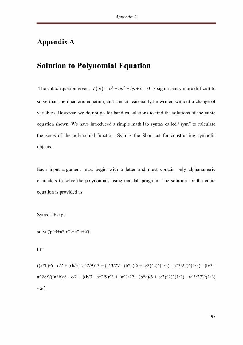
Appendix A
95
Appendix A
Solution to Polynomial Equation
The cubic equation given, 3 2 0f p p ap bp c is significantly more difficult to
solve than the quadratic equation, and cannot reasonably be written without a change of
variables. However, we do not go for hand calculations to find the solutions of the cubic
equation shown. We have introduced a simple math lab syntax called “sym” to calculate
the zeros of the polynomial function. Sym is the Short-cut for constructing symbolic
objects.
Each input argument must begin with a letter and must contain only alphanumeric
characters to solve the polynomials using mat lab program. The solution for the cubic
equation is provided as
Syms a b c p;
solve('p^3+a*p^2+b*p+c');
p1=
((a*b)/6 - c/2 + ((b/3 - a^2/9)^3 + (a^3/27 - (b*a)/6 + c/2)^2)^(1/2) - a^3/27)^(1/3) - (b/3 -
a^2/9)/((a*b)/6 - c/2 + ((b/3 - a^2/9)^3 + (a^3/27 - (b*a)/6 + c/2)^2)^(1/2) - a^3/27)^(1/3)
- a/3

Appendix A
96
P2=
(b/3 - a^2/9)/(2*((a*b)/6 - c/2 + ((b/3 - a^2/9)^3 + (a^3/27 - (b*a)/6 + c/2)^2)^(1/2) -
a^3/27)^(1/3)) - a/3 - ((a*b)/6 - c/2 + ((b/3 - a^2/9)^3 + (a^3/27 - (b*a)/6 + c/2)^2)^(1/2) -
a^3/27)^(1/3)/2 - (3^(1/2)*i*((b/3 - a^2/9)/((a*b)/6 - c/2 + ((b/3 - a^2/9)^3 + (a^3/27 -
(b*a)/6 + c/2)^2)^(1/2) - a^3/27)^(1/3) + ((a*b)/6 - c/2 + ((b/3 - a^2/9)^3 + (a^3/27 -
(b*a)/6 + c/2)^2)^(1/2) - a^3/27)^(1/3)))/2
P3=
(b/3 - a^2/9)/(2*((a*b)/6 - c/2 + ((b/3 - a^2/9)^3 + (a^3/27 - (b*a)/6 + c/2)^2)^(1/2) -
a^3/27)^(1/3)) - a/3 - ((a*b)/6 - c/2 + ((b/3 - a^2/9)^3 + (a^3/27 - (b*a)/6 + c/2)^2)^(1/2) -
a^3/27)^(1/3)/2 + (3^(1/2)*i*((b/3 - a^2/9)/((a*b)/6 - c/2 + ((b/3 - a^2/9)^3 + (a^3/27 -
(b*a)/6 + c/2)^2)^(1/2) - a^3/27)^(1/3) + ((a*b)/6 - c/2 + ((b/3 - a^2/9)^3 + (a^3/27 -
(b*a)/6 + c/2)^2)^(1/2) - a^3/27)^(1/3)))/2

Appendix B
97
Appendix B
Calculations of Cofactors and Determinant of the
Normalised Coupling Matrix, A
The normalised coupling matrix, A , is given by
11 12 13
1
12 22 23
2
13 23 33
3
1
1[ ]
1
e
e
e
jm p jm jmq
A jm jm p jmq
jm jm jm pq
1. 12cof A p
The cofactor, 12cof A p can be obtained by cancelling the first row and second
column of matrix, A , and this is shown as
12 13
( )
12
23 33
3
([ ]) ( 1) 1i j
e
jm jm
cof Ajm jm p
q
where i is a row number and j is a column number.

Appendix B
98
For this particular case 1i and 2j . Thus
12 12 33 13 23
3
12 33 12 12 13 23
3
12 33 12 12 13 23
3
1
1 ( . )
1
e
e
e
cof A p jm jm p m mq
jm jm jm p jm m mq
m m jm p jm m mq
2. 13cof A p
Similarly 13Cof A p may be calculated by cancelling the first row
and the third column of matrix, A , and this yields
12 13
( )
13
22 23
2
( 1) 1i j
e
jm jm
cof A pjm p jm
q
where 1i is the first row, and 3j is the third column of matrix, A . Thus
13 12 23 13 22
2
12 23 13 22
2
12 23 13 22
2
1( ( ))
1 ( ( ))
1 ( ( ))
e
e
e
cof A p m m jm jm pq
m m jm jm pq
m m jm jm pq

Appendix B
99
3. 11cof A
The cofactor, 11cof A p may be also computed by cancelling the first row and the
first column of matrix, A . This is shown as
22 23
2( )
11
23 33
3
1
( 1)1
ei j
e
jm p jmq
cof A p
jm jm pq
where 1i j is the first row and column of matrix, A .
Thus
2 3322
11 22 33 22 33
3 3 2
2
23
2 2 3
2
22 33 22 33
3 2 2 3
1 ( )
1 1 1 ( )
(
e e e
e e e
e e e e
mm pcof A p m m jm p j jm p p j
q q q
pm
q q q
p jm jm p m mq q q q
2 3322
23
3 2
)e e
mmm j j
q q
4. det A p
The determinant, det A p of the matrix, A is calculated as
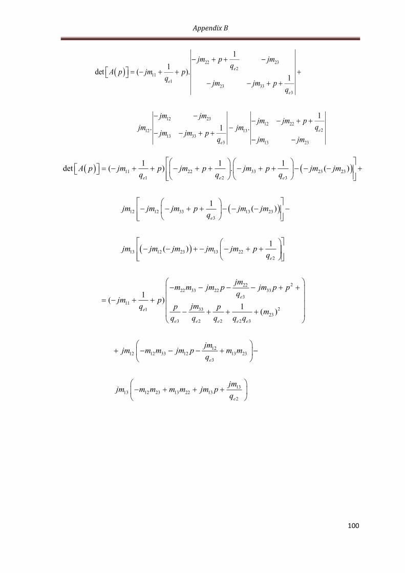
Appendix B
100
22 23
2
11
123 33
3
12 2312 22
212 13
13 33
3 13 23
1
1det ( ).
1
1
. .1
e
e
e
e
e
jm p jmq
A p jm pq
jm jm pq
jm jmjm jm p
qjm jmjm jm p
q jm jm
11 22 33 23 23
1 2 3
12 12 33 13 23
3
13 12 23 13 22
2
1 1 1det ( ) . ( )
1 ( )
1 ( )
(
e e e
e
e
A p jm p jm p jm p jm jmq q q
jm jm jm p jm jmq
jm jm jm jm jm pq
22222 33 22 33
3
11
233123
3 2 2 2 3
1212 12 33 12 13 23
3
13
13 12 23 13 22 13
2
1)
1( )
e
e
e e e e e
e
e
jmm m jm p jm p p
qjm p
jmq p pm
q q q q q
jmjm m m jm p m m
q
jmjm m m m m jm p
q

Appendix B
101
211 22 11
11 22 33 11 22 11 33 11
3 3
211 33 22 3311 11 22
11 23
2 2 2 3 1 1
2
33 3322
1 3 1 1 1 3 1 2 1 2 1 2 3
2
23
22 3
1
det
1
e e
e e e e e e
e e e e e e e e e e e e e
e
m m jm pA p jm m m m m p m m p jm p
q q
m m m mjm p jm jm pjm m
q q q q q q
jm p jmjm p p p
q q q q q q q q q q q q q
mm m
q
22 2 322
3 22 33
3 3
22 2 233
23 12 33 12
2 2 2 3
22
2 2 1312
12 13 23 13 22 13
3 2
( ) ( )
( )( )2 ( ) ( )
e e
e e e e
e e
jm p pp jm p jm p p
q q
jm p p pp m j m m m p
q q q q
mmj m m m j m m m p
q q
Thus, rearranging the equation above yields
3 2
11 22 33
1 3 2
3311 11 2211 22 11 33
3 2 1 1 1 3
3322
22 33
1 2 3 2 2 3
1 1 1det
1
1 1
e e e
e e e e e e
e e e e e e
A p p jm jm jm pq q q
jmjm jm jmm m m m p
q q q q q q
jmjmm m m
q q q q q q
2 2 2
23 12 13
211 33 22 3311 22 11
11 22 33 11 23
3 2 2 3 1
2 223 23322 12
12 33
1 3 1 2 1 2 3 1 3
( ) ( )
( )1 ( )
e e e e e
e e e e e e e e e
m m p
m m m mm m jmjm m m jm m
q q q q q
mjmjm mj m m
q q q q q q q q q
2
2 13
12 13 23 13 22
2
( ) 2 ( )
e
mj m m m j m m
q