Embed Size (px)
Citation preview

AEDC-TR-68-108
INVESTIGATION OF JET BOUNDARY
SIMULATION PARAMETERS
FOR UNDEREXPANDED JETS
IN A QUIESCENT ATMOSPHERE
6 ; ; .-'377
APR 1 6 1987
MAR 1 0 1389
R. D. Herron
ARO, Inc.
September 1968
This document has been approved for public release and sale; its distribution is unlimited.
'W"l "**? /*>■
U u. 1 J- 7
:i H-jS.
PROPULSION WIND TUNNEL FACILITY
ARNOLD ENGINEERING DEVELOPMENT CENTER
"AIR FORCE SYSTEMS COMMAND
ARNOLD AIR FORCE STATION, TENNESSEE
EBOOnSKZ 07 U. S. -** FCiiCS
4TJC LlBriLS P40000-£S-C-C001

mm When U. S. Government drawings specifications, or other data are used for any purpose other than a definitely related Government procurement operation, the Government thereby incurs no responsibility nor any obligation whatsoever, and the fact that the Government may have formulated, furnished, or in any way supplied the said drawings, specifications, or other data, is not to be regarded by implication or otherwise, or in any manner licensing the holder or any other person or corporation, or conveying any rights or permission to manufacture, use, or sell any patented invention that may in any way be related thereto,
Qualified users may obtain copies of this report from the Defense Documentation Center.
References to named commercial products in this report are not to be considered in any sense as an endorsement of the product by the United States Air Force or the Government.

AEDC-TR-6 8-108
INVESTIGATION OF JET BOUNDARY
SIMULATION PARAMETERS
FOR UNDEREXPANDED JETS
IN A QUIESCENT ATMOSPHERE
R. D. Herron
ARO, Inc.
This document has been approved for public release and sale; its distribution is unlimited.

AEDC-TR-68-108
FOREWORD
The research reported herein was sponsored by the Arnold Engi- neering Development Center (AEDC), Air Force Systems Command (AFSC), under Program Element 6540223F and is related to Project 8953, Task 895309.
The results of research presented in this report were obtained by ARO, Inc. (a subsidiary of Sverdrup & Parcel and Associates, Inc.), contract operator of the AEDC, AFSC, Arnold Air Force Station, Tennessee, under Contract F40600-69-C-0001. The work was performed from March 1965 to June 1967 under ARO Projects No. PW5728 and PW3517, and the manuscript was submitted for publication on April 18, 1968.
This technical report has been reviewed and is approved.
Carl E. Simmons Edward R. Feicht Captain, USAF Colonel, USAF Research Division Director of Plans Directorate of Plans and Technology
and Technology
li

AEDC-TR-68-108
ABSTRACT
An experimental and theoretical investigation was conducted to determine the degree of jet boundary simulation obtainable for under- expanded jets exhausting into a quiescent atmosphere. Tests were conducted with nitrogen, carbon dioxide, and helium gases, and theoretical boundaries were obtained by a method-of-characteristics solution. It was determined that the method-of-characteristics solu- tion accurately represents the experimental jet boundaries and that the matching of the parameters 6j and Mj/^ gives good boundary simulation for a wide range of jet conditions. Also a rapid, simple method for estimating jet boundary shape is developed from the method-of - characteristics results.
111

AEDC-TR-68-108
CONTENTS
page
ABSTRACT iii NOMENCLATURE viii
I. INTRODUCTION 1 II. THEORETICAL BOUNDARY CALCULATIONS
2. 1 Latvala's Approximation 2 2.2 Method-of-Characteristics Solution 2 2. 3 Jet Boundary Viscous Mixing Region 4
III. APPARATUS AND TEST PROCEDURE 3. 1 Te"st Hardware and Procedure 5 3. 2 Flow Visualization 6 3.3 Pressure Probe Traverses 7
IV. RESULTS AND DISCUSSION . . 4. 1 Theoretical Jet Boundaries 7 4. 2 Experimental Results 8 4. 3 Analysis of Other Simulation Parameters 9 4.4 Simulation Parameters 5j and M^/^ 10 4.5 A Rapid Method for Estimating the Inviscid
Boundary Location 11 V. CONCLUDING REMARKS 12
REFERENCES 12
APPENDIXES
I. ILLUSTRATIONS
Figure
1. 18-Inch Test Cell Installation 17
2. Test Nozzle Configuration 18
3. Model Installation in the 18-Inch Test Cell 19
4. Typical Photographs of Experimental Jet Plumes for 7Mi2/ßi = 14
a. CO2, 6j = 60 deg, 9N = 20 deg 36 min 21
b. N2, öj = 60 deg, 0N = !0 deg 21
c. He, 6j = 58 deg 28 min, 9^ = 10 deg ; 21
5. Typical Jet Density Distribution 23
6. Comparison of Boundaries Determined by the "Glow Discharge" Technique with the Pressure Measured by a Traversing Probe
a. N2, r/re = 18.22 24 b. C02, r/re = 8. 18 25
AEDC-TR-68-108
Figure Page
7. Range of Nozzle Area Ratio and Exit Pressure Ratio for Jets with Constant Values of YMI
2//3I
and 6j = 60 deg a. TM^/ßi =10 26 b. TM^/ß! =14 27 c. 7Mi2/3!, = 18 28 d. 7M12/ß1 =22 29
8. Comparison of Jet Boundaries as Determined by the Latvala Approximation
a. 7M12/ß1 = 10, 6 j = 60 deg 30 b. 7M1
2/j3i = 14, 6j = 60 deg 31 c. TM^/JSJ = 18, Sj = 60 deg 32
38
d. 71^2/0! = 22, 6j = 60 deg 33
9. Comparison of Jet Boundaries as Determined by a Method-of-Characteristics Solution
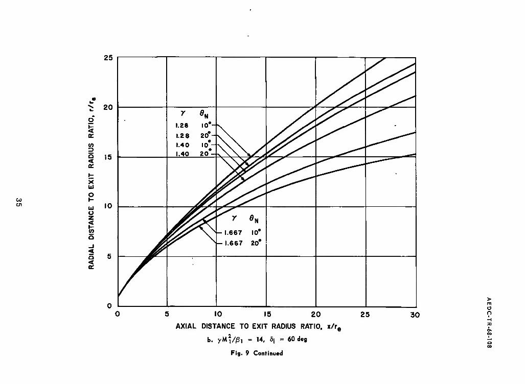
a. 7Mi2/ßr= 10, 6j = 60 deg 34 b. 7M12/ß1 = 14, 6j = 60 deg 35 c. 7M12/ß1 = 18, 6j = 60 deg 36 d. 7M12/ß1 = 22, 6-j = 60 deg 37
10. A Comparison of Experimentally Determined Jet Boundaries with a Method-of-Characteristics Solution for 7M1
2/ß1 = 14 a. CC-2, 0N ■ 10 deg, 5j = 60 deg b. C02, ON = 20 deg 36 min, Sj = 60 deg 39 c. N2, 0N
= 10 deg, 6j = 60 deg 40 d. N2, ©N = 20 deg 36 min, 6j = 60 deg 41 e. He, % = 10 deg, 6j = 58 deg 28 min 42 f. He, % = 20 deg 36 min, 6j = 61 deg 56 min. . . 43
11. A Comparison of Experimentally Determined Jet Boundaries with a Method-of-Characteristics Solution for 7M12/ßj = 18
a. N2, 0N = 10 deg, Sj = 60 deg 44 b. N2, 0N = 20 deg, öj = 60 deg 45 c. He, 0N = 10 deg, 6j = 60 deg 46 d. He, 0N = 20 deg, 6j = 60 deg 47
12. Location of Equilibrium Gas Saturation Conditions for an Expansion from the Experimental Stagnation Temperatures and Pressures
a. C02 48 b. N2 49
VI

AEDC-TR-68-108
Figure Page
13. Effect of the Nozzle Exit Reynolds Number on the Location of the Experimental Jet Boundary Relative to the Calculated Inviscid Boundary at x/re = 20. ... 50
14. Comparison of Jet Boundaries for Other Proposed Simulation Parameters
a. 7Mj/ßj =4.55, 6j = 60 deg 51 b. 7Mj2/ßj =4.45, Pj/p„ = 345 52 c. 7Mj2/ßj =4.55, Pj/Po, = 345, öj = 60 deg ... 53
15. Summary of Calculated Boundaries Presented in Figure 9
a. 0N = 10 deg, öj = 60 deg 54 b. 0N = 20 deg, 6j = 60 deg 55
16. Correlation of Jet Radii from Figure 15 at a Fixed Axial Distance to Exit Radius Ratio
a. x/re = 10 56 b. x/re = 18 57
17. Range of Nozzle Area Ratio and Exit Pressure Ratio for Jets with Constant Values of M1/7
a. öj = 75 deg 58 b. 6j = 60 deg 59 c. öj = 45 deg " 60
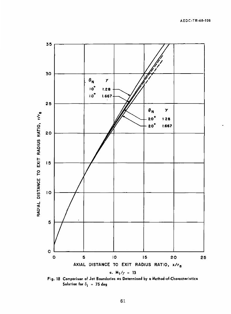
18. Comparison of Jet Boundaries as Determined by a Method-of-Characteristics Solution for öj = 75 deg
a. Mx/7 = 13 61 b. Mi/7 = 10 62 c. Mi/7 = 7 63 d. Mi/7 = 5 64
19. Comparison of Jet Boundaries as Determined by a Method-of-Characteristics Solution for öj = 60 deg
a. M1/7 =13 65 b. Mi/7 =10 66 c. M1/7 = 7 67 d. M1/7 =5 68
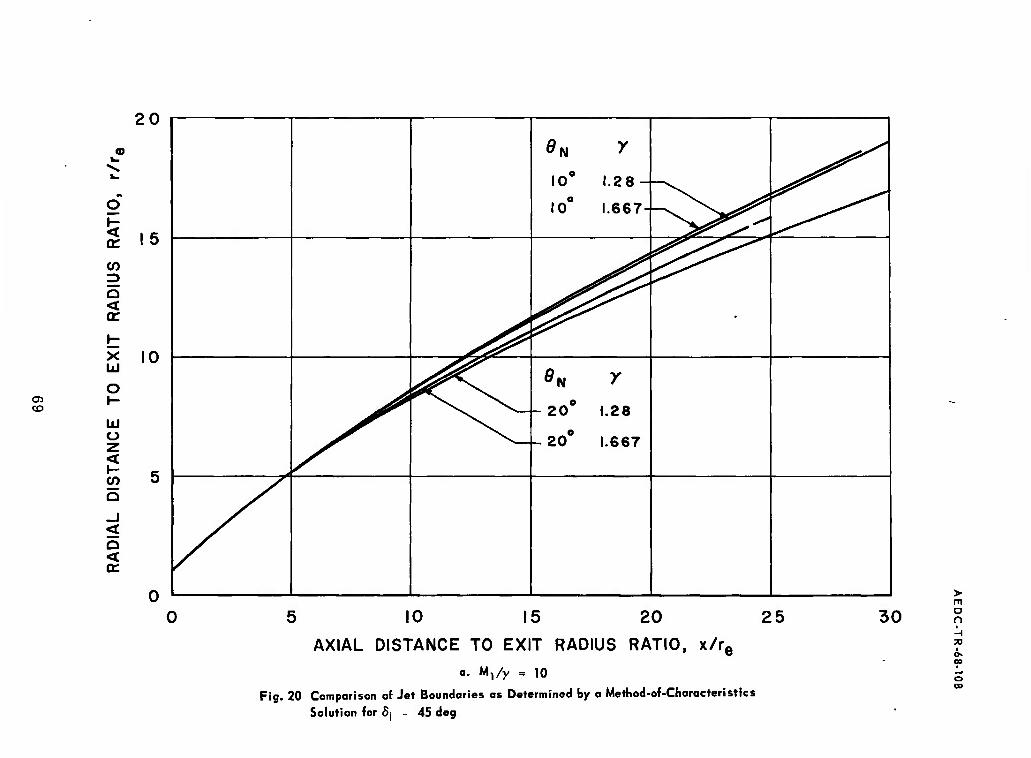
20. Comparison of Jet Boundaries as Determined by a Method-of-Characteristics Solution for öj = 45 deg
a. M1/7 =10 69 b. M1/7 = 7 70 c. M1/7 = 5 71
Vll

AEDC-TR-68-108
Figure Page
21. Effect of the Boundary Initial Angle on the Jet Radius at a Given Axial Distance for Nozzles with 0£j = 10 deg. . . .
a. x/re = 5 72 b. x/re = 10 73 c. x/re = 18 74 d. x/re = 25 75
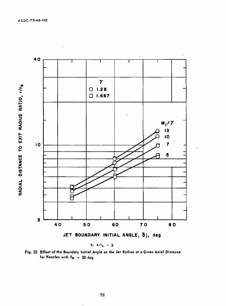
22. Effect of the Boundary Initial Angle on the Jet Radius at a Given Axial Distance for Nozzles with 6N = 20 deg
a. x/re = 5 76 b. x/re = 10 77 c. x/re = 18 78 d. x/re = 25 79
H. TABLES
I. Flow Properties of Computed Jets Matching the Simulation Parameters TM^/ßi and gj 80
II. Flow Properties of Computed Jets Matching the Simulation Parameters MJ/Y and fij 81
NOMENCLATURE
As/A* Nozzle spherical area ratio,
de Nozzle exit diameter
d* Nozzle throat diameter
2 1 + COS 0]\J
ij Distance along the nozzle wall measured from the throat to the nozzle exit
&l Distance measured from the nozzle exit along the inviscid jet boundary
M Mach number
n Distance measured normal to the inviscid jet boundary, positive outside the inviscid jet
p Pressure
Pp Pressure measured by the traversing probe
Vlll

AEDC-TR-68-108
X
ß
7
6H
>N
v
P
Jet radius
Nozzle exit radius
Temperature
Velocity at the nozzle exit
Distance from the nozzle exit measured along the nozzle axis, positive downstream
M2 - 1
Ratio of specific heats
Jet boundary initial angle relative to the nozzle axis
Nozzle half-angle
Coefficient of viscosity corresponding to static conditions at the nozzle exit
Prandti.-Meyer angle
Density
J
SUBSCRIPTS (Reference circled symbols in sketch below)
1 Jet boundary conditions
j Nozzle exit conditions
t Total or stagnation conditions
oo Atmospheric or ambient conditions
IX

AEDC-TR-68-108
SECTION I INTRODUCTION
In recent years, much interest has arisen in the structure and properties of highly underexpanded rocket or ramjet exhaust plumes. This interest has been created by problems such as heating and eros- ion of adjacent surfaces, radar and communication signal interference, separation of flow over the vehicle, and radiation emitted by the large exhaust plumes. Studies of and attempts to obtain solutions to these problems have led to the construction of high altitude test facilities and the adaptation of some existing facilities. Methods used for the experimental simulation of the full-scale jets vary in complexity from the use of small cold-gas jets to an almost exact duplication of the full- scale jets. The degree of similitude required and/or used depends on the particular problem under investigation and is discussed in Ref. 1. However the tremendous vacuum pumping capacities required and the complexity and cost of hot rocket tests frequently dictate that studies be conducted with small jets of cold gases.
One jet characteristic frequently desired is that the boundary of the experimental jet duplicates that of the full-scale jet. In an early study, Love (Ref. 2) concluded that for slightly underexpanded jets (P-i/p<n from 1 to 10) good boundary simulation was obtained if the initial angle, 6j, of the jet boundary was matched. Goethert (Ref. 3) later proposed matching the parameters Sj and 7Mj2/ß. for highly under- expanded jets. Pindzola (Ref. 4) concluded that better simulation could be obtained by matching 6A and YM^/JS^ where the Mach number is now based on the jet boundary conditions rather than the nozzle exit condi- tions as proposed by Goethert.
The objective of the investigation reported herein was to determine the degree of jet boundary simulation obtained using Pindzola's param- eters and to determine if other simulation parameters might prove more useful. The investigation included both experimental and theoretical studies of the jet boundaries. Values of the simulation parameters 6j and 7Mi2/ßi were selected that were representative of underexpanded jet plumes, and tests were conducted with nitrogen (N2), helium (He), and carbon dioxide "(CO2) jets at constant values of the parameters. In addition, jet boundaries were calculated for several sets of simu- lation parameters by an approximate method and also by a method-of- characteristics solution.
From these studies it was determined that although the parameters 6j and TMi^/ßi gave good jet boundary duplication, better duplication

AEDC-TR-68-108
could be obtained by matching the parameters 6j and MI/Y. Also, a simple method was developed for rapidly predicting the jet boundary for a wide range of conditions.
SECTION II
THEORETICAL BOLTOARY CALCULATIONS
2.1 LATVALA'S APPROXIMATION
The approximation used by Pindzola (Ref. 4) for the original evaluation of the simulation parameters 6j and TMi^/ßi Was devel- oped by Latvala in Ref. 5. Latvala's approximation is based on quasi- one-dimensional relations and the assumption of isentropic, radial flow from the nozzle. It is an adaptation of a method presented by Adams on and Nichols in Ref. 6, but uses a spherical rather than a planar area to define the flow area of the jet.
The approximate solution starts with the known initial angle of the jet, 6j, calculated from
8. = Vl - v. - eN (l)
The condition of constant pressure along the jet boundary is then used to determine the changes in jet boundary angle required to com- press the flow and balance the pressure decrease caused by the one- dimensional flow area increase. The relation between turning angle and pressure change is given by the Prandtl-Meyer expansion relation
Ap yM* (Ai/) + higher order terms in \v (2)
which is identical (except for sign of Ay) to the expression for a com- pression through an oblique shock wave, up to and including the term in (Av)2. It is apparent then that two jets that have the same value of the coefficient YMi^/ßi could be expected to have the same pressure change-deflection angle relation within the limits of the linearization of Eq. (2). This therefore gives rise to the use of 6j and TMi2/^ as the jet boundary simulation parameters.
2.2 METHOD-OF-CHARACTERISTICS SOLUTION
The most accurate method existing for calculating the properties of an inviscid expanding jet is the method of characteristics. However, the accuracy obtained in the actual application depends on factors such

AEDC-TR-68-108
as the knowledge of the actual flow properties at the start of the cal- culation (the nozzle exit), the frequent assumption of neglecting the jet boundary shock, and the nonideal behavior of the gas. Also, the accuracy is limited by the computer program used because of the finite mesh size rapidly becoming larger as the solution proceeds downstream. In most applications, the effects of the viscous mixing on the jet bound- ary must be considered.
Application of method-of-characteristics solutions to determine the free jet boundaries have been made by several authors (Refs. 2, 5, and 7 through 12). Among these, Refs. 2, 5, and 7 included limited experimental data for sonic nozzles or low to moderately expanding jets from supersonic nozzles. Experimental determination of jet boundaries for highly underexpanded jets has been prevented by the density limitations of conventional optical instrumentation; therefore a "glow discharge" technique was used in Ref. 12. The method-of- characteristics solution was also compared in Ref. 13 with experi- mental data on the internal structure of jets expanding into a vacuum. In general, the above authors found the method of characteristics to reasonably predict the jet boundaries and flow properties, within its inherent limitations. A good survey of some of the exact and approxi- mate solutions for the jet structure has been given by Adamson (Ref. 14).
The computer program used for the present calculations was developed by the Lockheed Missile and Space Corporation for use with the IBM 7090 computer. 'This program computes the supersonic flow properties of a gas discharging from an underexpanded nozzle into either a quiescent atmosphere or a hypersonic free stream. Ideal gas relations, oblique shock relations for the boundary shock, and the axisymmetric method of characteristics are employed. A complete description of the program is given in Ref. 15, and only the principal assumptions and the techniques used in the application of the program are given here.
Jet boundaries presented in this report were computed on an IBM 360/50 computer for the following conditions and assumptions:
1. For the case of a quiescent atmosphere only.
2. Nozzle exit flow properties were computed by the program from ideal gas, one-dimensional flow relations utilizing point source flow (spherical areas). Specific heat ratios of 1. 28, 1.40, and 1. 667 were used for both the nozzle and the jet flows. The value

AEDC-TR-68-108
of 1. 28 used for comparison with experimental tests of CO2 corresponds to excitation of one of the four modes of the molecular vibration.
3. The method-of-characteristics computation starts on the spherical nozzle exit surface; normally 4Q, points were used for the origin of the characteristic net.
4. Flow properties for the initial expansion around the nozzle lip are computed from Prandtl-Meyer relations. Approxi- mately 1. 5-deg increments were used for the Prandtl - Meyer expansion system.
Recently a new program has been developed (Ref. 16) which in- cludes equilibrium reacting gas mixtures and a wider variety of flow field problems. A comparison of this program with some experimental data is given in Ref. 17. These comparisons include limited data from jets with sonic nozzles and with low exit pressure ratio supersonic nozzles. In general the comparisons were considered very good. This program (Ref. 16) is currently being adapted to the AEDC computer system.
2.3 JET BOUNDARY VISCOUS MIXING REGION
The velocity gradients normal to the flow direction in the interior of the jet are usually small, and therefore viscosity effects are neg- lected. The jet interior structure can then be calculated by the method of characteristics as described previously. However, the gradients are not negligible at the jet boundary, and effects of viscous mixing must be considered.
Ideally, the inviscid boundary can be determined and the flow proper- ties at the inviscid boundary used to determine the corresponding mixing region flow properties. The viscid mixing solution can then be super- imposed on the inviscid jet solution to define the physical jet. This pro- cedure is probably valid if the mixing region is small compared to the jet radius and if no chemical reactions occur.
The growth of the turbulent mixing region was calculated for the conditions corresponding to the present experimental tests using the method given by Bauer in Ref. 18. The type of mixing considered is turbulent, two-dimensional, compressible, isobaric, isoenergetic, and without an initial boundary layer. It is of significance to note that for the high jet boundary Mach numbers considered in this report, the mixing region thickness and velocity distributions are almost identical for all jets. For these, the edges of the mixing regions are: n/re/jHi/re = 0.13 for the outer edge and -0. 01 for the inner edge.

AEDC-TR-68-108
SECTION III APPARATUS AND TEST PROCEDURE
3.1 TEST HARDWARE AND PROCEDURE
The experiments reported in this report were conducted in an 18-in. test cell connected to a six-stage steam ejector. The test cell installation is shown in Fig. 1, Appendix I. Test gases were heated by a resistance-type heater and expanded through conical nozzles into the test cell. Test nozzles had throat diameters of approximately 0. 1 in.
Two sets of values of the simulation parameters were selected as being representative of typical underexpanded jet plumes:
5j = 60deg, yMj/ft = 14
and , Sj = 60deg, ylA\tßx = 16
These values of the simulation parameters were maintained constant, and tests were conducted with pure gases in 10- and 20-deg half-angle conical nozzles. Nitrogen, CC^, and He gases were tested at a simu- lation parameter value of 14; N2 and He were tested at a value of 18. Different values of ambient pressure and nozzle area ratio were required for each of 10 different nozzles in order to maintain the selected values of the simulation parameters.
Since each gas required a different nozzle area ratio to match the selected value of the simulation parameters, testing began with CO2 (the largest nozzle area ratio). The nozzle exit was then cut off to give the required area ratios for N2 and He. The configurations of the various test nozzles are shown in Fig. 2.
Possible effects of nozzle boundary layer, jet viscous mixing, gas condensation, specific heat ratio variation, and gas nonequilibrium could not be precisely evaluated beforehand; therefore, tests were conducted over a range of stagnation pressures from 100 to 400 psia; and, temperatures from 100 to 1000°F. At each test condition, cell ambient pressure was adjusted to give the required jet expansion to match the chosen values of the simulation parameters. All tests were conducted under steady-state conditions.

AEDC-TR-68-108
3.2 FLOW VISUALIZATION
A glow discharge technique was used to illuminate the jet plume so that it could be photographed, since the required test cell pres- sures were well below the sensitivity limit of conventional optical techniques. The glow discharge technique, previously used for jet plume studies in Ref. 12, utilized an electrically charged probe approximately 5 in. downstream of the nozzle exit. This electrical charge was supplied by Osram®ignition unit originally designed for igni- tion of 2000-w high-pressure xenon arc lamps. This unit is rated at 40 kv-RF at 18 ma.
Very small amounts of N2 or CO2 gas were bled into the 'upstream end of the test cell through a manifold ring. This technique, discussed in Ref. 12, provides a fine adjustment of the test cell pressure but was used primarily to give a color contrast between the jet and the ambient atmosphere. This is achieved by inbleeding CO2 when using N2 as the jet gas and vice versa. Although the color of the gas discharge varies somewhat with pressure level and gas temperature, the generally blue glow of the CO2 improves the boundary contrast between the pink glow of the N2. Carbon dioxide was also used for the inbleed gas in the tests with He. Figure 3 gives an interior view of the test cell showing the electrical probe and the gas inbleed manifold installation.
The illuminated plumes were photographed with a 35-mm camera equipped with a 50-mm lens. Ektachrome® ER-ASA160-Tungsten Balance film was used, and exposure times were normally 1/30 sec. Data were obtained at several exposure settings at each test condi- tion, with f/4 generally giving best results. Optimum exposure varied with jet stagnation temperature and pressure. No change in boundary location could be detected as a result of a change in exposure.
Typical photographs of the jet plumes are shown in Fig. 4. Also shown in the figure are the boundary points that were selected as the experimental data as well as the theoretical method-of-characteristics solutions. The original color positives were projected, and both top and bottom boundaries were measured and averaged to give the plotted data presented later in this report.
The light emitted by the excited gas has been shown to be nearly a linear function of the gas density for the pressure range of these tests (Ref. 19). For the highly expanded plumes investigated, the gas density very rapidly decreases downstream of the nozzle exit as typically shown in Fig. 5. However, downstream at the boundary shock (which lies close to the inviscid boundary) an order-of-magnitude rise in density occurs,

AEDC-TR-68-108
giving the bright band of light. The outer edge of this band was meas- ured as being the jet boundary. Near the nozzle exit the jet boundary tends to disappear, particularly for the CO2 and the N2 jets. The disappearance of the boundary may be attributed to a number of effects, including the shorter viewing path through the three-dimensional jet at the smaller axial distances, glow phenomena electrode effects, and the nozzle boundary layer.
3.3 PRESSURE PROBE TRAVERSES
To confirm that the visible boundary did in fact closely represent the physical jet, limited pressure probe traverses were made through the CO2 and N2 jet-boundaries. These traverses were made parallel to the jet axis and do not necessarily give the pitot pressure. The probe tip was 1/8 in. in diameter and is shown in Fig. 3. Results of these tests are shown in Fig. 6. Generally good agreement is shown between the jet boundary indicated by the pressure probe traverse and that obtained with the glow discharge technique.
SECTION IV RESULTS AND DISCUSSION
4.1 THEORETICAL JET BOUNDARIES
Jet boundaries were calculated by the Latvala approximation and by the method of characteristics for values of the simulation param- eters of 6j = 60 deg and 7Mi2/ßi equal to 10, 14, 18, and 22. Boundaries were computed corresponding to nozzle half-angles of 10 and 20 deg with jet specific heat ratios of 1. 667, 1.40, and 1. 28. These calculations cover a very wide range oi possible operating conditions, as shown in Table I (Appendix ID and in Fig. 7.
Results of the calculations by the Latvala approximation are shown in Fig. 8, and by the method of characteristics in Fig. 9. Note that since the Latvala approximation starts after the jet expan- sion to ambient pressure, the calculations shown in Fig. 8 are valid for all values of the nozzle half-angle, 0jj. These computations show the Latvala approximation to give almost exact boundary duplication for all conditions calculated, whereas the method of characteristics predicts substantial divergence between boundaries, especially at the lower values of 7Mi2/ßj. Somewhat closer boundary duplication for

AEDC-TR-68-108
the method-of-characteristics solutions is obtained by adding the nozzle half-angle, 0]sj, as an additional parameter. Also note that the bound- aries with a specific heat ratio, 7, of 1.667 diverge the greatest, and that for most applications good boundary simulation would be obtained for axial distances of 10 to 15 nozzle exit radii by using air (7 = 1.4) to simulate a hot rocket (7 = 1. 28).
4.2 EXPERIMENTAL RESULTS
Results of experimental tests with CO2, N2, and He for 7Mi2/ßi = 14 are shown in Fig. 10, and tests with N2 and He for 7M -p/ß\ = 18 are shown in Fig. 11. Carbon dioxide was not used in the tests with 7Mi2/ßi = 18 because of the very low ambient pressures and the very large nozzle area ratios (Fig. 7) required. Data symbols are only shown for the portions of the boundaries for which a distinct boundary could be deter- mined from the projected negatives and are shown as read, without any fairing or smoothing. Also shown are the theoretical boundaries as calculated by the method of characteristics. Since tolerances in machining the test nozzles will cause errors in the jet initial angle, 6j, the actual initial angle is shown and the theoretical boundaries recalcu- lated if the test value deviated more than 1 deg from the desired 60 deg. The experimental data generally lie slightly outside the method-of- characteristics solutions, as would be expected for a viscid fluid. However, little effect of gas stagnation temperature or pressure is observed, indicating little effect of nozzle boundary layer, gas con- densation, or changes in the boundary viscous mixing. The exception is the data for N2 at high stagnation pressures.
The boundary increase shown for the high stagnation pressure N2
is real, as previously shown by the pressure probe data in Fig. 6a, and not just an apparent change caused by the flow visualization technique. Such a change could be caused by gas condensation in the test nozzles or in the jet plume. The very large rates of gas expansion in the noz- zles and in the plumes would give a substantial amount of supersatura- tion before condensation would occur. However, as shown in Fig. 12, even equilibrium condensation in the test nozzles is possible only for the C02 at 300°F and condensation with the 100°F, 100-psia stagnation test conditions would occur far before condensation at the 1000°F, 500-psia conditions. The close agreement of the nitrogen boundaries at low stagnation pressure test conditions and for all conditions with C02 shows that gas condensation in the jet plume either does not occur or has no effect on the measured jet boundaries.
An analysis was made of the experimental K2 data for possible effects of the nozzle boundary layer or changes in the jet boundary mixing region. The maximum change in the nozzle exit flow properties that can be caused
8

AEDC-TR-68-108
by the displacement thickness of a turbulent boundary layer will cause only a 0. 5-deg increase in jet boundary initial angle, 6j. This change is not sufficient to cause the boundary location increase shown for the high stagnation pressures. However, an analysis of the deviation of the experimental boundaries from the method-of-characteristics solutions shows excellent agreement when the data are correlated by the Reynolds number at the nozzle exit. This correlation is shown in Fig. 13, which also includes the data with He and CO2. The Reynolds number is based on the length along the nozzle wall from the throat to the exit and the viscosity data of Ref. 20 for He and of Ref. 21 (extrapolation required for lowest temperatures) for N2 and CO2. The critical Reynolds num- ber indicated in Fig. 13 is almost identical with the values given in Ref. 22 for flat plates with comparable Mach numbers. A somewhat higher critical Reynolds number would be expected for the nozzle flow because of the favorable pressure gradient; however, the choice of the proper length for nozzle flows is uncertain. Also shown in Fig. 13 are the edges of the turbulent mixing region calculated as described in Section 2. 3, which gives good agreement with the data at the higher Reynolds numbers. Although it would be attractive to attribute the smaller jet boundaries at the lower Reynolds numbers to a laminar jet boundary, Ref. 23 would indicate laminar boundary thicknesses com- parable to or thicker than that for a turbulent boundary. However the velocity profile assumed in Ref. 23 may not be valid at the very high Mach numbers of the experimental jet boundaries. It is significant that the inviscid method of characteristics does give a good representation of the physical jet boundary, although insufficient knowledge of the vis- cous mixing process and the factors affecting it may not always allow an absolute correction for the mixing.
In general, excellent agreement'is obtained between the inviscid method-of-characteristics solutions and the experimental data. It is therefore believed that the validity of this program with the inputs and techniques used has been confirmed and that a comparison of simu- lation parameters can now be made using the method-of-characteristics calculations for the jet boundaries rather than requiring experimental measurements.
4.3 ANALYSIS OF OTHER SIMULATION PARAMETERS
Although the proposed simulation parameters 6j and 7Mi2/j3i do provide good simulation for most cases of practical interest, they do not^appear to be the completely general tool that one desires. There- fore with the method-of-characteristics program confirmed as a method of calculating the physical jet boundary, a limited analysis of
9

AEDC-TR-68-108
some of the other proposed simulation parameters was made. Among the parameters investigated were:
1. yMj2//3j and 6j
2. yMj2/|3j and pj/p» (Ref. 3)
3. yM-j2//3j, pj/Pooand6j (Ref. 1)
Results of this limited analysis are shown in Fig. 14. Of the sets of parameters studied none except the third set gave results as good as the yMi^/lßi and 6j suggested in Ref. 4. However it should be noted that the third set requires the matching of three quantities rather than two, and is therefore a more restricted simulation.
The use of the third set of simulation parameters shown above implicitly specifies a value of 0jj. The required value of 0N is there- fore shown in Fig. 14c which presents a set of boundaries calculated for the given set of simulation parameters.
4.4 SIMULATION PARAMETERS 5, AND Mi/y
A rapid analysis of any other parameter in combination with 6j can be made from the existing method-of-characteristics solutions for 6j = 60 deg. This is done by observing the variation of the jet bound- ary radial locations at a fixed axial station as compared to changes of the parameter under study. Ideally then, boundary locations for all calculations should give a smooth progression for the changes of the selected parameter. A summary of the calculated boundaries from which the analysis can be made is shown in Fig. 15.
The analysis described above was made on several parameters involving combinations of Mi and y. This analysis shows excellent correlation of the boundary location when 6i and Mj/y are used as the simulation parameters. A slight improvement in correlation can be gained by also duplicating 0^ as a third parameter. Sample results of this analysis are shown in Fig. 16. Excellent correlation of the boundary locations is shown.
Based on the preceding analysis, additional boundary calculations were made by the method of characteristics to determine the range of applicability of the parameters 6j and Mj/y. Calculations were made for the following conditions:
10

AEDC-TR-68-108
1. Jet boundary initial angles, 6j, of 45, 60, and 75 deg.
2. Simulation parameter M1/7 values of 5, 7, 10, and 13.
3. Specific heat ratio of 1. 28 and 1. 667.
4. Nozzle half-angle, 6-^, of 10 and 20 deg.
The very wide range of conditions covered by these calculations is shown in Table II and in Fig. 17.
Results of the calculations are shown in Figs. 18, 19, and 20. Excellent agreement between the boundaries is obtained over the very wide range of conditions investigated. Some improvement is obtained by including the nozzle half-angle, ©N, as a third simulation parameter. Also note that the boundaries are presented for two extreme cases of the specific heat ratio, 1. 28 and 1. 667 only; for most practical applica- tions using diatomic gases, the boundaries would show even better agreement.
4.5 A RAPID METHOD FOR ESTIMATING THE INVISCID BOUNDARY LOCATION
The close correlation of jet boundaries with the simulation param- eters 6j, Mi/7, and 0N gives rise to a very simple method of rapidly estimating the inviscid boundary location. Boundary locations at fixed axial stations are shown in Figs. 21 and 22 as a function of the jet initial angle, 6j, and the parameter M1/7 for nozzle half-angles of 10 and 20 deg. The estimating procedure is as follows:
1. From Eq. (1) the initial angle of the jet, 6-j, is calcu- lated. This establishes the slope of the boundary at the nozzle exit.
2. Calculate M^/7 from the known stagnation pressure, ambient pressure, and specific heat ratio.
3. The boundary location r/re can then be located at x/re = 5, 10, 18, and 25 from Fig. 21 for 0N
= 10 deg or Fig. 22 for #N = 20 deg. This provides up to five known points plus the initial angle, 6j, and is normally enough for an accurate boundary. If desired, additional figures similar to Figs. 21 and 22 can be constructed at any x/re from Figs. 18, 19, and 20.
4. The small correction for other values of 0jj can be made by a comparison of the boundaries at 10 and 20 deg.
11

AEDC-TR-68-108
SECTION V CONCLUDING REMARKS
The theoretical and experimental investigation of jet boundary simulation parameters for underexpanded jets in a quiescent atmos- phere indicate the following conclusions:
1. Experimental jet boundaries are in excellent agreement with the inviscid jet boundaries as determined by the method of characteristics.
2. Pindzola's parameters (öj and YM^/ßj) give good boundary simulation for 10 to 15 nozzle exit radii for most applica- tions using air (y - 1.4) to simulate a hot rocket (7 = 1. 28).
3. However, the use of 6j and M1/7 provides excellent bound- ary duplication over a wider range of conditions and to much larger axial distances. In addition, a slight improvement in the correlation can be gained by also duplicating #N as a third parameter.
4. A procedure developed from the method-of-characteristics solutions gives a rapid, simple method for estimating the jet boundary shape for jets with boundary initial angles from 45 to 75 deg.
REFERENCES
1. Pindzola, M. "Jet Simulation in Ground Test Facilities. " AGARDograph No. 79, November 1963.
2. Love, Eugene S., Grigsby, Carl E., Lee, Louise P., and Woodling, Mildred J. "Experimental and Theoretical Studies of Axisymmetric Free Jets. " NASA TR R-6, 1959.
3. Goethert, B. H. and Barnes, L. T. "Some Studies of the Flow Pattern at the Base of Missiles with Rocket Exhaust Jets. " AEDC-TR-58-12 (AD302082), October 1958.
4. Pindzola, M. "Boundary Simulation Parameters for Under- expanded Jets in a Quiescent Atmosphere. " AEDC-TR-65-6 (AD454770), January 1965.
5. Latvala, E. K. "Spreading of Rocket Exhaust Jets at High Altitudes." AEDC-TR-59-11 (AD215866), June 1959.
12

AEDC-TR-68-108
6. Adamson, T. C. Jr. and Nicholls, J. A. "On the Structure of Jets from Highly Underexpanded Nozzles into Still Air." Journal of the Aerospace Sciences, Vol. 26, No. 1, p. 16, January 1959.
7. Vick, Allen R., Andrews, Earl H. Jr., Dennard, John S., and Craidon, Charlotte B. "Comparisons of Experimental Free- Jet Boundaries with Theoretical Results Obtained with the Method of Characteristics. " NASA TN D-2327, June 1964.
8. Eastman, D. W. and Radtke, L. P. "Two-Dimensional or Axially Symmetric Real Gas Flows by the Method of Characteristics, Part III: A Summary of Results from the IBM 7090 Program for Calculating the Flow Field of a Supersonic Jet. " The Boeing Company, Seattle, Washington, Document No. D2-10599, December 1961.
9. Wang, C. J. and Peterson, J. B. "Spreading of Supersonic Jets from Axially Symmetric Nozzles. " Jet Propulsion, Vol. 28, No. 5, p. 321, May 1958.
10. Moe, Mildred M. and Troesch, B. Andreas. "The Computation of Jet Flows with Shocks. " Space Technology Laboratories, Inc. , STL-TR-59-0000-00661.
11. Andrews, Earl H. , Jr., Vick, Allen R., and Craidon, Charlotte B. "Theoretical Boundaries and Internal Characteristics of Exhaust Plumes from Three Different Supersonic Nozzles." NASA TN D-2650, March 1965.
12. Prunty, C. C. "Jet Spreading Characteristics at Pressure Alti- tudes of 180,000 to 260,000 Feet." AEDC-TR-64-95 (AD603341), August 1964.
13. Cassanova, R. A. and Stephens on, W. B. "Expansion of a Jet into Near Vacuum. " AEDC-TR-65-151 (AD469041), August 1965.
14. Adamson, Thomas C., Jr. "The Structure of the Rocket Exhaust Plume without Reaction at Various Altitudes. " The University of Michigan, Institute of Science and Technology, Report No. 4613-45-T (AD421447), June 1963. .
15. Prozan, R. J. "PMS Jet Wake Study Program IMSC External Flow Jet Wake Program VN10. " Lockheed Aircraft Corporation Report No. LMSC 919901, 9 October 1961.
16. Prozan, R. J. "Development of a Method of Characteristics Solu- tion for Supersonic Flow of an Ideal, Frozen, or Equilibrium Reacting Gas Mixture. " Lockheed Missiles and Space Company Huntsville Research and Engineering Center, Technical Report LMSC/HREC A782535, April 1966.
13

AEDC-TR-68-108
17. Ratliff, A. W. "Comparisons of Experimental Supersonic Flow Fields with Results Obtained by using a Method of Character- istics Solution. " Lockheed Missiles and Space Company, Huntsville Research and Engineering Center, Technical Report LMSC/HREC A782592, April 1966.
18. Bauer, R. C. "Characteristics of Axisymmetric and Two- Dimensional Isoenergetic Jet Mixing Zones. " AEDC-TDR- 63-253 (AD426116), December 1963.
19. Muntz, E. P. and Marsden, D. J. "Electron Excitation Applied to the Experimental Investigation of Rarefied Gas Dynamics," Rarefied Gas Dynamics, Proceedings of the Third Inter- national Symposium on Rarefied Gas Dynamics, Held at the Palais De L'Unesco, Paris in 1962, Vol. II, 1963.
20. Keesom, W. H. Helium, pp. 106-110, Elsevier Publishing Company, New York, 1942.
21. Hilsenrath, Joseph, Beckett, Charles W., et al. Tables of Thermo- dynamic and Transport Properties of Air, Argon, Carbon Dioxide, Carbon Monoxide Hydrogen, Nitrogen, Oxygen, and Steam, p. 191 and p. 357, Pergamon Press, 1960.
22. Schlichting, Hermann. Boundary Layer Theory. Fourth Edition, p. 438. McGraw-Hill Book Company, 1960.
23. Bauer, R. C. "An Analysis of Two-Dimensional Laminar and Turbulent Compressible Mixing. " AIAA Journal, Vol. 4, No. 3, March 1966, pp. 392-395.
14

AEDC-TR-68-108
APPENDIXES
I. ILLUSTRATIONS II. TABLES
15

> m O
A E D cl o
7 707 -66 1 TO
-■-■>>?- OS
Fig. 1 18-Inch Test Cell Installation

AEDC-TR-68-108
r30°
FLOW »
*e \
■
t- 0.125 inches
yM^/01
14
18
% Gas d*
inches inches
As/A*
20°36" C02 0.0989 0.6470 44.21
N2 0.2818 8.39 1 1
He 1 0.1344 1.91
10°0' co2 0.1026 0.4680 20.97
N2 0.2181 4.55 ' He ' 0.1254 1.51
20°0« N2 0.1039 0.3585 12.28
1 He 1 0.1570 2.35
10°0' N2 0.1026 0.2630 6.62
1 1 He 1 I 0.1310 1.64
Fig. 2 Test Nozzle Configuration
18

CD
n
OS
Fig. 3 Model Installation in the 18-Inch Test Cel

a. CO2, 5| * 60 deg, 6H - 20 deg 36 min
CO
b. N2, Sj = 60 deg,
ON = 10 deg
c He, 5j = 58 deg 28 min, 0U = 10 deg 2
Fig. 4 Typical Photographs of Experimental Jet Plumes for y^-\/ß\ - 14
o 1
-t
I
o 00

to GO
< (r to
Q <
X UJ
O »- UJ Ü
to Q _l <
<
5 10 15 20 25
AXIAL DISTANCE TO EXIT RADIUS RATIO, x/re
Fig. 5 Typical Jet Density Distribution
r>

AEDC-TR-68-108
SOLID SYMBOLS CORRESPOND TO
BOUNDARY LOCATIONS FROM
GLOW DISCHARGE TECHNIQUE O x 2 10
< K
UJ DC
CO CO ill <E a
o
|
< »- to
id CD O CC 0.
CO
UJ
8
6
pt, psfa Tt, °F O 100 100 D 450 100 0 100 1000
oo
• C i c
\o
ij i h
Jl {
i 4 10 15 20 25
AXIAL DISTANCE TO EXIT RADIUS RATIO, x/re
a. N2, r/re = 18.22
Fig. 6 Comparison of Boundaries Determined by the "Glow Discharge" Technique with the Pressure Measured by a Traversing Probe
30
24

AEDC-TR-68-108
O
K
a a.
< cr UJ or CO CO Ui (C a
SOLID SYMBOLS CORRESPOND TO
BOUNDARY LOCATIONS FROM
GLOW DISCHARGE TECHNIQUE
I 2 z
CO
ui 8 a. C9
CO K UJ
5 i-
8 12 16 20
AXIAL DISTANCE TO EXIT RADIUS RATIO, x/r,
b. COfc r/r„ = 8.18
Fig. 6 Concluded
25

AEDC-TR-68-108
30,000
I 10,000 —
< K
UJ ec 3 CO co
a. o
£ 1,000 CO
< o
100
30
"" 1 ■ I I | I I ■T—r i ■ i <i
r = i.28
I ! I I I I I I .1.1.1
10
NOZZLE SPHERICAL AREA RATIO, A,/A
100 300
a. yM,/^ = 10
Fig. 7 Range of Nozzle Area Ratio and Exit Pressure Ratio for Jets with Constant
Values of yM, //3, and 5= = 60 deg
26

AEDC-TR-68-108
30,000 "" 1 I I I I I I ■>—I ' I I I M
8 10,000
o i- <
« IÜ
«9
U ffi
O I-
X toJ
UJ _J N N O
BH = 10°
1,000 1.28
SOLID SYMBOLS CORRESPOND TO
CONDITIONS FOR EXPERIMENTAL JETS
100
30 I.I.I
10
NOZZLE SPHERICAL AREA RATIO, A»/A
100 300
b. yMiV/Bi = 14
Fig. 7 Continued
27

AEDC-TR-68-108
30,000
8 10,000 —
o
to u K a. o
I CO
t- z w ffl
< O
t X U
Id -I N N O
1,000 —
100 —
30
1 ' 1 1 1 ' 1 < 1 1 ' 1 ' U 1 ' 1 |
— -
— . — — - -
_ *NS«0^^ \ —
— s^ \y = i.28 -
- -
^~ \l.40 ^ —
— _ - - — - - \l.667 ^/ - — — - - — -
- SOLID SYMBOLS CORRESPOND TO
CONDITIONS FOR EXPERIMENTAL JETS -
—
1 I 1 . 1,1,1 1 .1.1.1.1 1
-
10 4
NOZZLE SPHERICAL AREA RATIO, A,/A
c. yM,2/|8, = 18
Fig. 7 Continued
100 300
28

AEDC-TR-68-108
30,000 1 1 1 l f I I 1 1 1—' I ■ I l I
0N='° r = i.28
g 10,000
CL*
K
ui K
CO CO UI ac a o
£ 1,000
ca 3 < o
u -I Nl N O 100
90 J I ■ 1 ■ I i I _i I .lil.
10
NOZZLE SPHERICAL AREA RATIO, AJ/A"
100 300
d. yMi//3, = 22
Fig. 7 Concluded
29

25
20
CO o
<
CO
Q < tr
x
o
to Q
_l < <
15
10
■
>^v^ ̂ r
\— 1.667 N— 1.40 N— 1.28
o n ■ -i
10 15 20 25 30
AXIAL DISTANCE TO EXIT RADIUS RATIO, x/re
.2 a. yM\/ßi 10, Sj - 60deg
Fig. 8 Comparison of Jet Boundaries as Determined by the Latvala Approximation

25
20
co
<
CO
a <
X UJ
UJ o z
CO
o _l <
< a:
15
10
< y \— 1.667 \- 1.40
^^1.28
10 15 20 25 30
AXIAL DISTANCE TO EXIT RADIUS RATIO, x/rg
b. yM*//S, = 14, 5, - 60 deg
Fig. 8 Continued
> m O n I -a a 09'

25
GO to
20
< ac
Q < or
X Ld
LÜ Ü
CO
o -I < <
15
10
- 2*-1.667 <^-l.40 ^1.28
n
00
10 15 20 25 30
AXIAL DISTANCE TO EXIT RADIUS RATIO, x/re
c. yM,2//3, = 18, 5j - 60 deg
Fig. 8 Continued

25
00 00
20
»- < er (0
Q < er
x
U o z < I-
Q
< Q <
15
10
f r S— 1.667 ^— 1.40 ^— 1.28
5 10 15 20 AXIAL DISTANCE TO EXIT RADIUS RATIO, x/re
d. yM,2//3! = 22, 8, = 60 deg
Fig. 8 Concluded
25 30
> m o n i
-i

25
20
00
< DC
OT
< a:
UJ
O
Ul ü Z
12 CO
a < or
15
10
y *N 1.28 10-
1.28 20°- 1.40 IO->
o 1,40 20->
r *N ^_^_
^-1.667 10°
^-1.667 20°
n
as
10 15 20 25 30
AXIAL DISTANCE TO EXIT RADIUS RATIO, x/re
a. yM*//S, = 10, Sj = 60 deg
Fig. 9 Comparison of Jet Boundaries as Determined by a Method-of-Characteristics Solution
25
"£ 20
GO
<
CO
a < or
x UJ
o UJ Ü
CO
a
< tr
15
10
y dH
1.28 10°-
1.2 8 20°- 1.40 10°- 1.40 20°-
-
- 1.667 10°
- 1.667 20°
5 10 15 20
AXIAL DISTANCE TO EXIT RADIUS RATIO, x/re
b. yM*//3, = 14, S| = 60deg
Fig. 9 Continued
25 30 n
o 00

25
CO
20
< tr (O
a < DC
X Ul
Ul o z ? Q
-I < 5 <
15
10
^>
1.28 10°- 1.28 20°- 1.40 10°- 1.40 20*-
r eH
-1.667 10°
-1.667 20°
o n
10 15 20 25 30
AXIAL DISTANCE TO EXIT RADIUS RATIO, x/re
e. yMi/j8, = 18, S| = 60 deg
Fig. 9 Continued

25
CO. -Jl
- 20 o h- < DC
(/>
Q
2 15
x
Ul o
I Q
10
y ON
1.28 10° ~ 1.28 20°- 1.40 10° - 1.40 20°-
y eN
-1.667 10°
-1.667 20°
^
,'
5 10 15 20
AXIAL DISTANCE TO EXIT RADIUS RATIO, x/re;
«•• Y*\/ß\ = 22, $i = 60 deg
Fig. 9 Concluded
25 30
$

25
00 CO
w 20 o" t- < a: CO 3 a < 15 a. h- X ÜJ
O r-
o 10 32 < r- co Q
_l < O 5 < DT
<X /
A D
p/
X
Ay
* x \ -THEORETICAL, X = 1.28
pf, psia Tt, F
A/ D 200 A 400
C fU
420 1000
a o
00
0 5 10 15 20 25
AXIAL DISTANCE TO EXIT RADIUS RATIO, x/re
a. C02, du = 10 deg, 5, = 60 deg
Fig. 10 A Comparison of Experimentally Determined Jet Boundaries with a Method-of-Characteristics
Solution for Y^/ßi M '*
30

25
20
00 CD
< or CO => a <
X UJ
UJ u
to a
a < a:
15
D - THEORETICAL, Y- 1.28
Pt, psia Tt. F
- D 100 300
-
7^ ^- RADIUS OF PRESSURE
PROBE TRAVERSE
□ 200 345 0 300 970 A 500 950
A/
5 10 15 20 25
AXIAL DISTANCE TO EXIT RADIUS RATIO, x/re
b. C02, ON = 20 deg 36 min, 8\ = 60 deg
Fig. 10 Continued
30
> m O n

25
20
4*. o
< fr CO
Q <
x UJ
o I-
LÜ Ü
CO
Q
<
<
15
10
D o^y A D O,
■» o. O >
A D oX^l
□ vy A \s D y
A °/\ D -THEORETICAL, 7 = 1.40
AD
Pf> psia T|i F
O 100 100
D 500 100 0 100 1000 A 500 1000
o n
00
o 09
5 10 15 20 25
AXIAL DISTANCE TO EXIT RADIUS RATIO, x/re
c. N2, (>H = 10 deg, Sj = 60 deg
Fig. 10 Continued
30

25
^
<
<n
a < or
x u o
UJ o z
CO
o _I < Q < DC
20
15
10
D
□ O
RADIUS OF PRESSURE PROBE TRAVERSE *.
D ~i L/
-&*- -\j-^m
° <*^ o ^ Sy^
6 >
6/ -THEORETICAL, X = 1.40
ay pt, psia Tt, F
O 100 100
D 500 100 0 100 1000
5 10 15 20
AXIAL DISTANCE TO EXIT RADIUS RATIO, x/re
d. N2, ON = 20 deg 36 min, b\ = 60 deg
Fig. 10 Continued
25 30 n
■TO ■

25
tv3
<
CO
Q
Q:
X UJ
o H
UJ o z
CO
Q
Q
oc
20
15
10
• ^^-***C3
0
- THEORETICAL, X =1.667
Pt, psia Tt, °F
□ 300 0 100 A 300
100 1000 1000
> m O n i -i
■
o 00
5 10 15 20
AXIAL DISTANCE TO EXIT RADIUS RATIO, x/re
e. He, 0N - 10 «leg, <5j = 58 deg 28 min
Fig. 10 Continued
25 30

25
*" 20
a: CO
< 15
00
X UJ
id u
to
< Q < or
10
-<?£"
- THEORETICAL, Y = 1.667
Pt, psia Tt. °F
□ 300 0 100 A 300
100 1000 1000
5 10 15 20
AXIAL DISTANCE TO EXIT RADIUS RATIO, x/re
f. He, On =20 deg 36 min, Sj =■ 61 deg 56 min
Fig. 10 Concluded
25 30
> m o
CO

25
- 20
<
Q < IT
X UJ
o r-
UJ u
CO
o
<
15
10
D A 0 O P
6 A n 0 y
A
oD
A
A
-THEORETICAL, y=i.4o
8 Pt, Psia
O 200 D 400
100 100
0 200 1000 A 400 1000
•
> m O n i H A]
O 00
10 15 20 25 30
AXIAL DISTANCE TO EXIT RADIUS RATIO, x/re
a. N2, On - 10 deg, o, 60 deg
Fig. 11 A Comparison of Experimentally Determined Jet Boundaries with a Method-of•Character!sties
Solution for yM j/ß] - 18

25
20
CJ1
5 a: en 3 O <
X UJ
UJ Ü
i Q
-I <
< a:
15
10
a A^
D
OS 0 /
TurnecTir AI y - i An
Pt, psia Tt, °F
O 200 250
D 400 100 0 200 1000
D
10 15 20 25 30
AXIAL DISTANCE TO EXIT RADIUS RATIO, x/re
b. N2, On = 20 deg, $| =■ 60 deg
Fig. 11 Continued
a n
70
09
o CD

25
Ü cc (/> 2 a <
X Ul
o
UJ o z Ü CO
o _l < a <* cc
20
15
10
^
0
' 0
9^i -THEORETICAL, 7=1.667
pf, psia Tt, °F O 100 100 0 100 1000
o/
(y
a n
oo
5 10 15 20 25
AXIAL DISTANCE TO EXIT RADIUS RATIO, x/re
c. He, ON = 10 deg, 5j = 60 deg
Fig. 11 Continued
30

25
« v 20
< or en
Q <
X id o UJ Ü z
to o _J < <
15
10
& .^?
-THEORETICAL, /=l.667
v^T) pt, psia Tt, °F O 100 100 0 100 1000 A 300 1000
/o
5 10 15 20
AXIAL DISTANCE TO EXIT RADIUS RATIO, x/re
d. He, 0N = 20deg, 5j - 60 deg
Fig. 11 Concluded
25 30 a n
o 00

AEDC-TR-68-108
to -I
<
Id 0T 3 CO CO Id <r Q.
O
r- <
CO
o u
I CO
10 -
10
r l 1 1 i I ' .
GAS SATURATION POINTS "™
— Pti PSia Tf. °F ~"
- O D
too 200
300 300
-
0 300 1000 ~
A 500 1000 -
.-■ -
NOZZLE EXIT
ÖN yM,2//3,
10° 14
20° 14
•
i
-s
-
-
ISENTROPIC EXPANSION FOR r = 1.28 \^ ™"
r4 , i i
10 " -
3.0 4.0 6.0 7.0 5.0
MACH NUMBER
o. co2
Fig. 12 Location of Equilibrium Gas Saturation Conditions for an Expansion
from the Experimental Stagnation Temperatures and Pressures
48

AEDC-TR-68-108
- 10
a o" Ü
10 in ui
a.
NOZZLE EXIT
eN XM|2//3
10° 14
10° 18
20° 14
20° 18
10
(9
CO
en 10
ISENTROPIC EXPANSION FOR 7 = 1.4
GAS SATURATION POINTS Pf. P»ia Tp
o 100 100
D 500 100
0 100 1000
A 500 1000
10 -5 _L _1_ 3.0 4.0 5.0 6.0 7.0
MACH NUMBER
b. N2
Fig. 12 .Concluded
8.0 9.0 10.0
49

o n
en o
<
K. U Q. X Li
IE < Q Z o m o o CO
>
o
tu o z
CO o
CO
Q <
x Id
Id
N O •* 7
GAS
O N2
D He
A C02 <n/re MEASURED ATx/re = IO)
OPEN SYMBOLS Tt = MINIMUM
SOLID SYMBOLS Tt = MAXIMUM
T T^
O OUTER EDGE
-Q.
#TP-*
"O"
Ä
TURBULENT
MIXING REGION,
SEE SECTION 1A
INNER EDGE THEORETICAL INVISCID BOUNDARY
I ■ I I.I.I I
NOZZLE EXIT REYNOLDS NUMBER,
10 70
xlO -5
Fig. 13 Effect of the Nozzle Exit Reynolds Number on the Location of the Experimental Jet Boundary Relative to
the Calculated Inviscid Boundary at x/re = 20
o-

25
20
ai
or
Q 4 or
X ÜJ
UJ u
(0 a _i < a < or
15
y °H 1.28 10°.
1.40 10°- 1.667 10° -
r «N - 1.28 20°
• - 1.40 20 - 1.667 20V
5 10 15 20 25
AXIAL DISTANCE TO EXIT RADIUS RATIO, x/re
a. yMj/^j = 4.55, 5j - 60 deg
Fig. 14 Comparison of Jet Boundaries for Other Proposed Simulation Parameters
30 n
00

25
20
to
< or CO 3 Q < or
x UJ
UJ o z
CO a
< o < a:
15
- 1.28 10° - 1.40 10* - 1.667 10°
v<\ r
\S- 1.40 ^- 1.667
20° 20°
o n
at
5 10 15 20
AXIAL DISTANCE TO EXIT RADIUS RATIO, x/re
b. yMJV/ij = 4.45, p/p™ = 345
Fig. 14 Continued
25 30

25
20
<
w 2 15 O <
Id
U O
I o _J < < or
10
3 5
1.28 10.0° ■ 1.40 13.70° 1.667 19.0° ■
5 10 15 20
AXIAL DISTANCE TO EXIT RADIUS RATIO, x/re
«=• yMjV/Sj = 4.55, Pj/Poo = 345, 8, = 60 deg
Fig. 14 Concluded
25 30
> m O n
09

25
20
CM
<
CO
o < or
X IÜ
O r- Id Ü
<o Q
< or
I 5
10
REFERENCE TABLE X p0R
CASE NO. IDENTIFICATION
1 1 S Jf;/ CASE NO. 19/2^^3 v^^X^^X^® ^-'
S S yV^y"^ / ^""17 ^^" ^\^\
>i-<^ ^^^i
5
o n ■ H ^)
o 00
5 10 15 20
AXIAL DISTANCE TO EXIT RADIUS RATIO, x/re
a. ON = 10 deg, Sj = 60 deg
Fig. 15 Summary of Calculated Boundaries Presented in Figure 9
25 30

25
ai
20
< <r CO 3
a < a:
X UJ
LÜ CJ z 12 CO
Q
_l < < a:
15
10
REFERENCE TABLE I_ FOR
CASE NO. IDENTIFICATION
CASE NO. 2 0 / / 1 ^>
X S& l4 s/Z//r
7 S&SZ* ^^^^-^
^^" 10
12
4
6 *~
5 10 15 20
AXIAL DISTANCE TO EXIT RADIUS RATIO, x/re
b. ON =20 deg, Sj - 60 deg
Fig. 15 Concluded
25 30
> m a n
o 00

20
< rr
< er
en
Ul O
CO
Q
_l <
<
15
5 '0 UJ
20 -
XM,2//S|
O 10 D 14 A 18 0 22
2 4 6 8 10 12
BOUNDARY MACH NUMBER TO SPECIFIC HEAT RATIO, M,/y a. x/re = 10
Fig. 16 Correlation of Jet Radii from Figure 15 at a Fixed Axial Distance to Exit Radius Ratio
14
o n
70

25
20
Ul
< oc
co 3 Q < 15
t- X Ul
o »-
Ul 1 0 o z «I K CO o
_i < a 5 < ac
0N = IO- -^ 20° —v\ A
v\
<SJ
8j = 60°
/M2/£, O 10 D 14 A 18
0 22
6 8 10 12 14
BOUNDARY MACH NUMBER TO SPECIFIC HEAT RATIO, M,//
b. x/re = 18
Fig. 16 Concluded
> m o n
o 09

AEDC-TR.68-108
100,000
< et
V)
o
I 09
I- z UJ
CD 3 <
o
X Hi
ID -I N N O
10,000
1,000
100
1—' I 1] ' I
I ■ 111 10
1—I I I I I I
M,/r
A S
D 7
O 10
b 13
I.I.I
100
NOZZLE SPHERICAL AREA RATIO, A&/A*
a. Sj == 75 deg
Fig. 17 Range of Nozzle Area Ratio and Exit Pressure Ratio for Jets with Constant Values of M^y
58

AEDC-TR-6B-108
30,000
^ 10,000 —
o
V) in ui
is 1,000 v>
z t
bl
CD 2 <
o »-
X UI
UI -I 100 N IM O
30
T 1 1 ' I l I ' I 1 1 1 i I l I > 1
I , hlii -L 1 i I ■!
10 100 NOZZLE SPHERICAL AREA RATIO, A,/A*
b. & = 60
300
Fig. 17 Continued
59

AEDC-TR-68-108
10,000
a.
in
K a.
2 at
UJ
CD 2 <
1,000
100 -
N N o
10
I ' I ' I
Id
I ■ I ' I ■ I
J ■ I ■ I ■ 1.1
I ' I ' I
1 I.I.I 10 100
NOZZLE SPHERICAL AREA RATIO, A, /A*
1,000
c. Ö: 45deg
Fig. 17 Concluded
60
AEDC-TR-68-108
35
30
25
< a: V)
< a.
x
ÜJ o
Q
a < or
20
15
10
10° 1.28 -
10° 1.667-
Mrr /// /
eu r -20° 126
- 20° 1.667
0 5 10 15 20
AXIAL DISTANCE TO EXIT RADIUS RATIO, x/re
a. M,/y = 13
Fig. 18 Comparison of Jet Boundaries as Determined by a Method-of-Characteristics Solution for 5j = 75 deg
25
61

AEDC-TR-68-108
35
30
25
<x a:
O <t tr
t x UJ
ill o z < </> a
20
15
I '0
ON 7
10° 1. 28 -
10« 1.667-
9N Y
-20° 1.28
-20° 1.667
i I
/
5 10 15 20
AXIAL DISTANCE TO EXIT RADIUS RATIO, x/re
b. M,/y = 10
Fig. 18 Continued
25
62

AEDC-TR-68-108
35
30
25
o
K 10
Q <
x 1Ü
UJ o z < <0
o
20
15
^T t
*N r O
10 1.2 6 -
10° 1.667-
ON r -20° 1.26
-20° 1.667
1 i
5 10 15 20
AXIAL DISTANCE TO EXIT RADIUS RATIO, x/re
e. M,/y = 7
Fig. 18 Continued
25
63

AEDC-TR-68-108
30
25
<
xn 3 Q < 0C
X UJ
20
15
CO Q
a <
eH r 10° 1 28 -
10° 1.667- >^
eN r - 20° 1.28
-2 0° 1 667
5 10 15 20
AXIAL DISTANCE TO EXIT RADIUS RATIO, x/re
d. M,/y = 5
Fig. 18 Concluded
25
64

AEDC-TR-68-108
30
25
< DC
to r> Q <
X Id
P Ü z 15 to Q
_l <
< a:
20
15
c?N Y
10° 128-
10* 1.667
eN y
-20° 1.2 8
-20° 1.667
0 5 10 15 20 AXIAL DISTANCE TO EXIT RADIUS RATIO, x/re
a. M,/y = 13
Fig. 19 Comparison of Jet Boundaries as Determined by a Method-of-Characteristics Solution for S-. = 60 deg
25
65

AEDC-TR-68-108
30
25
20 1 er to
Q <
5 15 UJ
UJ o z <t
a 10
Q
a:
ON r 10« 1.28 —
10» 1.667-
6n r -20° 1.28
-2 0° 1.667
1 5 10 15 20
AXIAL DISTANCE TO EXIT RADIUS RATIO, */re
b. M,/y = 10
Fig. 19 Continued
25
66

AEDC-TR-68-108
30
25
to
Q <
X UJ
Ul o z < V) a
a <
20
15
10
9u y
10° 1.28-
10« 1.667-
^BH y -20* 1.28
-20° 1.667
5 10 15 20
AXIAL DISTANCE TO EXIT RADIUS RATIO, x/re
e. M,/y = 7
Fig. 19 Continued
25
67

AEDC-TR-68-108
30
25
< a: to
a <
X UJ
UJ o < t- £2 o
a < tr
20
15
10
10° 1.28 -
10° 1.667
- 20° 1.28
- 20° 1.667
5 10 15 20
AXIAL DISTANCE TO EXIT RADIUS RATIO, x/re
d. M!/}- = 5
Fig. 19 Concluded
25
68
20
OS CO
<
en
Q < tr
x UJ
o
o
<n o _J <
< IT
I 5
10
ON r 10* 1.28-
10° 1.667-
öN r - 20° 1.28
- 20° 1.667
5 10 15 20 25
AXIAL DISTANCE TO EXIT RADIUS RATIO, x/re
a. M,/y = 10
Fig. 20 Comparison of Jet Boundaries as Determined by a Method-of-Characteristies
Solution for S-. - 45 deg
30
> m o n H 73

2.0
-a o
5 a:
O <
X UJ
hi O
O
<
a:
15
10
ON 7
10° 1.2 8-
10° 1.667-
\ * \ ON 7
-20° 1.28
-20° 1.667
o n
to
5 10 15 20 25
AXIAL DISTANCE TO EXIT RADIUS RATIO, x/re
b. M,/y = 7
Fig. 20 Continued

20
a:
a <
X UJ
ÜJ ü z <
<
<
15
10
'
ON y 10° 1.28 — 10° 1.667-
~ w ̂
ON r - 20° 1.28 -20° 1.667
5 10 15 20 25
AXIAL DISTANCE TO EXIT RADIUS RATIO, x/re
C. Mi/y 5
Fig. 20 Concluded
30 > m O n
CO
o CD

AEDC-TR-68-108
40
< rr
a <
X LÜ
U
I CO
a
<
<
10
-
1 1—
y OI.28 D 1.667
1 1
-
- -
-
Q 13
>"x^ l0
y^n 7
f
-
— ^Q " - -
- -
- -
- -
-
i 1 ■
-
40 50 60 70 80
' JET BOUNDARY INITIAL ANGLE, 8j, deg
a. x/re = 5
Fig. 21 Effect of the Boundary Initial Angle on the Jet Radius at a Given Axial Distance for Nozzles with Q\\ = 10 deg
72

AEDC-TR-68-108
40
< AC
CO 3
Q <
l±J
o
UJ o z < I- tO 5
<
10
-
1
y O 1.28 G 1.667
1
-
- M,/y
Q 13 —
-
- "j~ -
- -
- bV^ -
- -
- -
- -
-
1 i I .. L J
-
40 50 60 70 JET BOUNDARY INITIAL ANGLE, 8j, deg
b. x/re = 10
Fig. 21 Continued
80
73

AEDC-TR-68-108
40
0)
< or
a < or
X ÜJ
o I-
ÜJ O z
CO
o _l <
<
10
1 ■ i
>ti 13 r
01.28 ^^Q 10
-
D 1.667
^O k8' -
^n 5
-
- -
- —
- -
- -
- -
- -
-
1 < i »
—
40 50 60 70
JET BOUNDARY INITIAL ANGLE, Sj, deg
c. x/re = 18
Fig. 21 Continued
80
74

AEDC-TR-68-108
40
<
CO
5 < or
x UJ
UJ u
CO
Q
5 0?
10
-
1 1 1 1
£\ 7
i
i iii
-
r 0 1.28 D 1.667
) l0 ^
-
- -
- -
- -
- -
- -
- —
-
i " I "
—
40 50 60 70
JET BOUNDARY INITIAL ANGLE, 8j, deg
d. x/re = 25
Fig. 21 Concluded
80
75
AEDC-TR-68-10B
40
< or CO
o < DT
X Id
UJ U z
to
<
< (IC
10
- 1 1 1 1
-
y
o D
1.28 1.667
— •
M,/y n i3
y/\P 10 /n 7
^3 5 -
-
- -
- -
- -
- -
-
1 i 1 1
-
40 50 60 70 80
JET BOUNDARY INITIAL ANGLE, Sj, deg
a. x/re - 5
Fig. 22 Effect of the Boundary Initial Angle on the Jet Radius at a Given Axial Distance for Nozzles with 6^ = 20 deg
76

AEDC-TR-68-108
40
< or
CO
5 < or
x tu
lü o z
<0
_J < 5 <
10
-
1 1 I 1 1
-
r O 1.28 D 1.667
M,/y
Q 13
jQ 7
-
-
- -
- -
- -
- -
- -
- -
-
1 1 1 i
4 0 50 6 0 70
JET BOUNDARY INITIAL ANGLE, 8j, deg
b. x/re = 10
Fig. 22 Continued
80
77

AEDC-TR-68-108
40
IE
CO 2 o < or
x UJ
UJ o
CO
o -I < 5
10
1 1 y 'M,/y O 1.28 D 1.667
Q 13
'J& io
r} 7
-
^<dB 5
-
- -
- -
- -
- -
- -
- -
-
1 1 ' 1
-
40 50 60 70
JET BOUNDARY INITIAL ANGLE, Sj, decj
c. x/re = 18
Fig. 22 Continued
80
78

AEDC-TR-68-108
40
g
tr to
ö < or H X U
O I-
bJ O Z
£ CO
o
< 5 <
10
-
1 1 1 I 1
M,// -
- Y
O 1.28 D 1.667
3 ,0 ^
jQ 7
5
-
- -
- -
- -
- -
- -
- -
-
I 1 1 i
-
40 50 60 70
JET BOUNDARY INITIAL ANGLE, Sj, deg
d. x/re = 25
Fig. 22 Concluded
80
79

AEDC-TR-68-108
TABLE I FLOW PROPERTIES OF COMPUTED JETS MATCHING THE
SIMULATION PARAMETERS }'M2/^, AND Sj
Case 6
de
6
1- r*l g
/P1 deg
10
r
1.28
Ml
7.747
A /A* s
3.399
Pj/P.
1 0 1 0 8.677 345.5
2 20 1.28 7.747 16.016 3.920 147.8
3 10 1.40 7.071 2.887 2.597 222.4
4 1
20 1.40 7.071 4.585 3.083 106.1
5 10 1.667 5.912 1.187 1.566 127.7
6 i 20 1.667 5.912 1.533 2.002 68.2
7 l 4 10 1.28 10.891 20.946 4.152 1806
8 20 1.28 10.891 44.896 4.836 646.7
9 10 1.40 9.949 4.786 3.129 921.9
10 20 1.40 9.949 8.472 3.740 384.5
11 10 1.667 8.338 1.441 1.904 396.0
12 1 ' 20 1.667 8.338 2.006 2.406 195.4
13 l 8 10 1.28 14.027 38.124 4.686 7331
14 20 1.28 14.027 90.935 5.509 2304
15 10 1.40 12.818 6.719 3.489 3010
16 20 1.40 12.818 12.807 4.201 1143
17 10 1.667 10.751 1.649 2.114 1003
18 ' 20 1.667 10.751 2.404 2.672 467.3
19 22 10 1.28 17.158 58.573 5.084 24714
20 20 1.28 17.158 151.41 6.024 7033
21 10 1.40 15.682 8.549 3.750 8279
22 20 1.40 15.682 17.197 4.545 2927
23 10 1.667 13.159 1.816 2.259 2200
24 1 20 1.667 13.159 2.733 2.861 982.5
80

oo
Case
25
26
27
28 29
30
31 32
33 34
35 36
37
38
39
40
41
42 43
44
6J' deg
75
TABLE II FLOW PROPERTIES OF COMPUTED JETS MATCHING THE
SIMULATION PARAMETERS M,/y AND d\
Mx/r
10
13
*
60
ON. deg
Y
1.28
Ml
6.400
As/A* M. J
2.405
Pj/P.
10 2.728 406.6 20 1.28 6.400 4.135 2.771 217.3 10 1.667 8.335 1.047 1.270 976.9 20 1.667 8.335 1.265 1.685 541.5 10 1.28 8.960 5.504 3.015 2201.0 20 1.28 8.960 9.418 3.468 1029.0 10 1.667 11.669 1.152 1.506 3580.0 20 1.667 11.669 1.469 1.934 1933.0 10 1.28 12.800 11.123 3.609 17527.0 20 1.28 12.800 21.404 4.171 7144.0 10 1.667 16.670 1.265 1.686 15806.0 20 1.667 16.670 1.679 2.141 8227.0 10 1.28 16.640 17.541 3.998 95410.0 20 1.28 16.640 36.465 4.645 35450.0 10 1.667 21 671 1.341 1.787 50404.0 20 1.667 21.671 1.820 2.262 25621.0 10 1.28 6.400 5.230 2.972 154.1 20 1.28 6.400 8.810 3.412 73.2 10 1.667 8.335 1.410 1.940 395.6 20 1.667 8.335 2.005 2.406 195.1
n
■
00

co to
TABLE II (Concluded)
Case 8j.
Mx/V oN. r Ml As/A* M.
J J 00 > m
deg
60
deg
10 1.28 8.960 3.723
O •
45 7 12.729 677.6
H
1 O CD
1
46 20 1.28 8.960 25.054 4.310 268.8 O CO
47 10 1.667 11.669 1.717 2.175 1373.0
48 ' 20 1.667 11.669 2.536 2.751 628.4
49 10 10 1.28 12.800 30.918 4.497 4345.0
50 - 20 1.28 12.800 70.991 5.268 1431.0
51 10 1.667 16.670 2.005 2.406 5694.0
52 1 20 1.667 16.670 3.116 3.057 2434.0
53 13 10 1.28 16.640 55.084 5.026 20419.0
54 20 1.28 16.640 140.680 5.948 5898.0
55 10 1.667 21.671 2.202 2.543 17450.0
56 ■ > • 20 1.667 21.671 3.536 3.250 7101.0
57 45 5 10 1.28 6.400 11.930 3.669 47.7
58 20 1.28 6.400 23.200 4.243 19.4
59 10 1.667 8.335 2.462 2.707 13.0
60 ' 20 1.667 8.335 4.085 3.475 50.6
61 7 10 1.28 8.960 36.667 4.650 160.9
62 20 1.28 8.960 86.839 5.463 51.0
63 10 1.667 11.669 3.224 3.109 399.5
64 ' 20 1.667 11.669 5.844 4.061 136.0
65 10 10 1.28 12.800 113.81 5.732 765.9
66 20 1.28 12.800 335.63 6.887 185.0
67 10 1.667 16.670 4.084 3.474 1479.0
68 1 • 20 1.667 16.670 8.035 4.625 443.7

UNCLASSIFIED Security Classification
DOCUMENT CONTROL DATA .R&D (Security classification ol Ulla, body of abstract and Indexing annotation must be entered when the overall report Is classified)
I ORIGINATING ACTIVITY (Corporate author)
Arnold Engineering Development Center ARO, Inc., Operating Contractor Arnold Air Force Station, Tennessee 37389
2a. REPORT SECURITY CLASSIFICATION
UNCLASSIFIED 2b. GROUP
N/A 3 REPORT TITLE
INVESTIGATION OF JET BOUNDARY SIMULATION PARAMETERS FOR UNDEREXPANDED JETS IN A QUIESCENT ATMOSPHERE
4 OESCRIPTIVE NOTES (Type ol report end Inclusive dates)
Final Report March 1965 to June 1967 5. AUTHOR(S) (First name, middle Initial, last name)
R. D. Herron, ARO, Inc.
8- REPORT DATE
September 1968 7«. TOTAL NO. OF PAGES
91 76. NO. OF REFS
23 6a. CONTRACT OR GRANT NO.
F40600-69-C-0001 b. PROJEC T NO.
Related to 8953, Task 895309 c'Program Element 6540223F
»a. ORIGINATOR'S REPORT NUMBER(S)
AEDC-TR-68-108
Ob. OTHER REPORT NO<S) (Any other numbers that may be assigned this report)
N/A 10 DISTRIBUTION STATEMENT
This document has been approved for public release and sale; its distribution is unlimited.
II. SUPPLEMENTARY NOTES
Available in DDC,
12. SPONSORING MILITARY ACTIVITY
Arnold Engineering Development Center (AETS), Arnold Air Force Station, Tennessee 37389
13. ABSTRACT
An experimental and theoretical investigation was conducted to determine the degree of jet boundary simulation obtainable for under- expanded jets exhausting into a quiescent atmosphere. Tests were conducted with nitrogen, carbon dioxide, and helium gases, and theoretical boundaries were obtained by a method-of-characteristics solution. It was determined that the method-of-characteristics solu- tion accurately represents the experimental jet boundaries and that the matching of the parameters 5j and M3.A, gives good boundary simulation for a wide range of jet conditions. Also a rapid, simple method for estimating jet boundary shape is developed from the method-of-characteristics results.
DD FORM ,1473 UNCLASSIFIED Security Classification

UNCLASSIFIED Security Classification
K EV WORDS ROLE WT ROLE
boundaries, jet
simulation techniques
jets, cold
jets, underexpanded
nitrogen
carbon dioxide
helium
UNCLASSIFIED Security Classification