Embed Size (px)
Citation preview

THE STEADY-STATE STRUCTURE OF RELATIVISTIC MAGNETIC JETS
Mark R Dubal Center for Relativity
The University of Texas at Austin Austin Texas 78712-1081
USA
Ornella Pantano Dipartimento di Fisica G Galilei
via Marzolo 8 35131 Padova Italy
June 1992
The steady-state structure ofrelativistic magnetic jets
Mark R DubaP and Ornella Pantano
I Center for Relativity University of Texas at Austin Austin Texas 78712-1081 USA
2Dipartimento di Fisica G Galilei via Marzolo 8 35131 Parlova Italy
Abstract The method of characteristics is used to study the structure of
steady relativistic jets containing a toroidal magnetic field component We assume
axisymmetry and perfect conductivity for the Buid Bows Oblique relativistic
magnetic shocks are handled using a shock fitting procedure The effects of the
magnetic field on the collimation and propagation of the jets are studied when the
external medium has a constant or decreasing pressure distribution Our parameter
study is confined to underexpanded jet Bows which have an ultra-relativistic equation
of stHk aud extremely supermagnetosonic bulk velocities The magnetic energy
density however may range from zero to extreme dominance These simulations are
therefore relevant to compact radio jet sources which exhibit superluminal motion
For slightly underexpanded jets propagating into a constant pressure external
medium the jet structure is quite periodic This periodicity is enhanced as the toroidal
field strength increases and the jet is strongly pinched Recollimation occurs whether
or not a toroidal field is present
When the jet propagates into an external medium of decr~asing pressure its
structure is very dependent upon the pressure gradient For a pressure law p ex z-2
where z is the distance from the jet BOurce the periodic structure is lost A nonshy
magnetic jet expands freely into the external medium and eventually comes into
pressure equilibrium with it A toroidal magnetic field cannot stop the jet from
expanding When p ex z-1 a semi-periodic structure is regained again this periodicity
is pArticularly noticeable when a strong toroidal field is present Also in this case
however the magnetic field cannot prevent the jet from expanding although it can
reduce greatly the rate at which it does so
1 2
1 Introduction
Many observations of extragalatic radio sources show highly collimated jets of gas
emanating from a central galaxy These outflows possibly composed ofelectron-proton
or electron-positron relativistic plasma sometimes exhibit apparent superluminal
lUotiollS implying relativistic bulk velocities with Lorentz factors of r 10 (Zensus
and Pearson 1987) The radiation from the jets is typically highly polarized and
follows a power-law spectrum indicating emission by the synchrotron process This
characteristic signature in turn denotes the presence of magnetic fields which in
many cases will play a significant role in determining the jet structure It is well
known for example that helical fields are capable of collimating plasma streams via
the pinch effect In the case of high power radio jets measurements of the X-ray
emissivity indicate that the pressure of the surrounding medium alone is insufficient
to confine the jet material and therefore magnetic fields must be invoked Moreover
with suitable magnetic field configurations it is possible to reduce the tendency of jet
disruption by Kelvin-Helmholtz and other shearing instabilities (Ferrari et al 1981)
This would then allow the formation of jets with lengths 103 times their beam
radius
Thus it is clear that both relativistic motion and magnetic fields play dominant
roles in determining the structure of astrophysical jets For this reason in this paper
we construct jet models by solving numerically the equations of special relativistic
magnetohydrodynamics (MHO) Our models necessarily have a number of simplifying
assumptions in particular we assume axisynunetric adiabatic and steady flows
with only a toroidal magnetic field component These assumptions require some
justification since real jets are three-dimensional lose energy by radiative mechanisms
and are turbulent to some extent
The two-dimensional nature ofour calculations is in the spirit of previous numerical
jet investigations (see for example Norman and Winkler 1984 Kassl et alI990abc)
ie that much can be learned from such simulations before moving onto more complex
and costly three-dimensional models Since our jet flows are stationary we do
not model instabilities axisymmetric or otherwise and therefore we are neglecting
completely the turbulent sheath that appears in the dynamical simulations of Norman
and Winkler and others Sanders (1983) Wilson and FaIle (1985) and F-dlle and
Wilson (1985) have investigated some of the properties of steady hydrodynamical jets
in the context of active galaxies Close to the jet source (or nozzel) steady flow is
thought to be a good approximation and therefore structures similar to those seen
in laboratory jets may appear Significant portions of the jet could be steady in
very high Mach number flows where large scale features respond slowly to pressure
changegt (Falle 1991) Thus our interest is in the average overall structure of the jet
ie the shape of the boundary and the positions of prominent features such as knots
and wiggles etc which vary slowly when compared to longitudinal flow time-scales
Perturbation theory also indicates that highly relativistic flows are stabilized against
shearing instabilities and that the presence of a magnetic field enhances this stability
still further (Ferrari et al 1981) Such results need to be verified in the non-linear
regime by the use of high resolution time-dependent relativistic MHO codes (Oubal
1991) however for the present we take the perturbation results to indicate that a
turbulent sheath (if one should form) plays a minor role in the overall jet structure
It would be interesting to test whether the steady jet models we construct are indeed
stable
Our approach to solving the relativistic MHO equations employs the method
of characteristics which requires that the system of partial differential equations
be purely hyperbolic This means that in steady two-dimensional flow the
(magnetoacoustic) Mach number must always be greater th~ one and no dissipative
terms can be handled The neglect of radiation losses in the jet flow is probably the
most serious approximation we make Wilson (1987b) has modelled relativistic steady
jets which are supersonic along their entire length Many shocks occur so that the gas
remains very hot and an ultra-relativistic equation of state (adiabatic index ( = 43)
is appropriate
The method of characteristics is well suited to studying the structure of steady
jets (Courant and Friedrichs 1948 Anderson 1982 for astrophysical applications see
Sanders 1983 and Daly and Marscher 1988) Its power lies in the fact that domains of
influence and dependence are modelled precisely and thus it is possible to treat waves
and discontinuities with high accuracy and efficiency A number of three-dimensional
characteristic techniques do exist however they are complicated and unlike the twoshy
dimensional ease the approach is not unique leading to hybrid schemes which often
lose the original power of the characteristic approach Therefore we have chosen to
3 4
start with the simpler two-dimensional problem
In principle our approach can handle any (axisymmetric) magnetic field
eoufiglllatioll however we include only a toroidal component he since this is the
most important one for collimation of the jet material (Kossl et al 1990c) It is
probable that he helps confine the jet at the nozzel exit (Wardle and Potash 1982) a
large he can stabilize the nozzel wall reducing incursion of wall material into the jet
and preventing its fragmentation by Kelvin-Helmholtz instabilities In addition hoseshy
pipe motions are reduced if the toroidal field is present in a surrounding conducting
sheath while beam disruption due to pinching modes is reduced if velocities are highly
relativistic Therefore the transverse field hi would be large near the nozzel and
would decay as the jet expands while the parallel field hilI increases due to the
shearing of hJ and dominates far from the source region A large hll at the source can
disrupt nozzel formation thus any asymmetry in the magnetic field configuration can
lead to one-sided jets (Benford 1987)
Taking into account the above discussion we aim to model high Mach number
compact jets close enough to the nozzel region that h dominates but sufficiently far
that the flow is already supermagnetosonic and therefore the gravitational influence
of the primary energy source (a black hole or otherwise) may be neglected
The plan of this paper is as follows In the next section we derive the characteristic
and compatibility equations for two-dimensional (axisymmetric) relativistic gas
flows with a single toroidal magnetic field component Following analogous work
in aerodynamic nozzel design we rewrite the equations in terms of quantities
which simplify the task of numerically solving these equations via the method of
characteristics Internal shocks can occur in the jet and their trajectories must be
tracked across the characteristic grid Therefore in section 3 we discuss the relations
between the values of the fluid variables on either side of a relativistic magnetic
oblique shock surface In section 4 the numerical approach is described in detail
Section 5 presents first some tests of the numerical code and then a parameter survey
of the general flow properties of the jets In particular we study the effect of an
increasingly large toroidal magnetic field on the initial expansion of the jet in constant
and decreasing pressure external mediums Some conclusions are drawn in section 6
5
2 The characteristic form of the Relativistic MHD equations
The equations which describe the flow of a perfectly conducting non-selfshy
gravitating relativistic fluid in the presence of a magnetic field are (i) the conservation
of baryons (ii) the conservation of energy-momentum and (iii) Maxwells equations
These may be written down as (eg Lichnerowicz 1967 Anile 1989)
Vo(pUO ) = 0 V o Toll =0 vo(uahll ullha) = 0 (1)
where p is the rest-mass density ua is the 4-velocity of the fluid Tall is the total
stress-energy tensor and ha represents the magnetic field The symbol Va denotes
the covariant derivative compatible with a flat spacetime metric goll For a perfect
(non-viscous) fluid the total stress-energy tensor takes the following form
1 Tall = (e +p + Ilhl2)uo ull + (p+ -llhI2 )gall Ihohll (lb)
2
where p is the isotropic fluid pressure e is the total fluid energy density I is the
magnetic permeability and Ih 12 = hoho gt O Note that the magnetic field is defined
such that U O ha 0 ie ha is orthogonal to the fluid 4-velocity The quantities p p
and e are all measured in the fluid comoving frame We are assuming isotropy and
infinite conductivity of the fluid so that the conductivity tldeg ll = tlOgoll with tlo -+ 00
and thus the field is frozen into the fluid The speed of light is taken to be unity
To complete the system of equations (1) we need to add an appropriate equation
of state of the form
p p(eS) (2)
where S is the specific entropy From Anile and Pennisi (1985) the system (1) may be
manipulated to give
e~uoVaP+ (e +p)VauQ = 0 (3a)
uOVoS = 0 (3b)
uOV hll- hOV ull + (ullhQ - e hlluQ) VaP = 0 (3c) a a P (e +p)
6
1 (e + p + plhl2)uaVaUfl phaVahll + (gall + 2uaull )phVah respectively Note that equation (3e) is satisfied trivially In equations (5d) and (5e)
1 + (e + p) [(e + p)gafl + (e + p - e~plhI2)uaull + phahfljVaP = 0 (3d) we have written w e +p + p( 1amp)2 which is the relativistic enthalpy of the fluid plus
the magnetic contribution Equation (5b) indicates that the fluid motion is adiabatic
however this condition is satisfied trivially by our choice of a perfect fluid equation of uaullVahll +Vaha 0 (3e) state and therefore (5b) can be discarded This does introduce a small error at strong
where shock fronts (Sanders 1983) but for weak or moderate shocks it is quite accurate The
remaining equations of the system (5) need to be solved for the unknown quantities p e~ = (oeop)s = lv~ and therefore e~ - 1 = (1 - v~)v~ = lc~ (4)
h v r and V Z bull In order to achieve this they will be written as compatibility equations
Here Vs is the thermal sound speed of the fluid and cs = rsvs where rev) = holding along characteristic curves
I - V2 )-12 is the usual special relativistic Lorentz factor We first look for combinations of (5) such that the new system has the form
In this paper we will use a cylindrical coordinate system (t r 9 z) but consider oU oU-+Amiddot-+B=O (6)only steady (oat = 0) axi-symmetric jets (ie no 9 dependence) with a single OZ Or
toroidal magnetic field component h Thus we can write ua = r1 vr0 vr) and where the state vector U T (p h v r VZ) We find that
ha =(OOhO) since uaha = O In this case there is never a time component of ha 2 rThen the system of equations (3) produces firstly from (3a) ph B)vrv z wr2vrB(1+ 1B) vv
v r -wr v B )
r Cvrv [1 +(A 1)Bvrv cwr2v -cwr2
(OP z lJp) ( )Jvr Jv v A= (7)t v-+v- +e+p -+-+shyp Or oz Or oz r 1wr2 v) ph(wr2v) vrv z
+ r 2 [
Jvr (Jvr ov) OVZ] -vr(wBc~) -phvr(wBc~) -AB r2vrvz~(BC~)(Vr)2_ + vrv _ + _ + (V)2_ = 0 (5a)Or oz Or oz and
and secondly from (3b)
B l = _r2vrvz -r2vrvr 0 __vr (8)(w Cw A ) r Br r Brv + v~ = o (5b)
whereThe t r and z components of equation (3c) are identically zero while the 9 component
gives 2c B = (rvr)2A r S 2+I -2-- A and C=~ (9)
Cs Cs BJlh r oh Z eP h rVPoh (A op) _
V a + v Tz - (e + p) v Or + v OZ - o (5c) In the expression for A we have defined the quantity CA = r AVA where
The r and z components of equation (3d) can be manipulated using the t component VA = [p(h)2wf2 (10)
to produce
r ovr Jvr) oh op which is the relativistic Alfven wave velocity in the rest frame of the fluid (see Appl wr2 v _ +vz _ + ph- + - =0 (5d)( or OZ Or Or and Camenzind 1988 Sloan and Smarr 1987) and The eigenvalues of the matrix A are found to be the double root
Jvz JvZ) oh op rwr2 vr_+v- +ph-+-=O (oo) Ao v( or OZ OZ oz V Z
(11)
7 8
representing the Alfven and slow magnetoacoustic waves and
MMZ plusmnJAM2 - A2 Aplusmn=--~(~M~z~)2--A~-- (12)
representing the fast magnetoacoustic waves Here Mi is the relativistic Mach number
ddiucd by M rvics and M2 = MiMi The system (6) is now re-written as
au au Imiddotmiddot-+Amiddotmiddotmiddot-+middotmiddotB deg with i = oplusmn (13)I az bulllOr
where Ii denotes the left eigenvectors which are found by solving Ii A Aii From
(7) the left eigenvectors are found to be first using (12)
Awr2vz Awr2v) Iplusmn ( 1lhplusmnJAM2 _ A2=F vAM2 _ A2 (14)
Then from (11) since Au is a double root there are two eigenvectors associated with
this solution we find
dz
I 0
( AIh8 v)
= 0 (A -1)r2vz w V Z I and II 0 = (A v)-rvZw 0-12 V Z
(15)
The compatibility equations are then
Ii dU + Ii Bdz = deg along dr Ai (16)
From (16) for the case of Ai = Aplusmn we have that
2 2d + hdh8 plusmn Awr v dv Awr v dv z
P I VAM2 _ A2 =F JAM2 _ A2 2 r
Awr [ AV] v+-- vzplusmn -dz=O (17)B JAM2 _A2 r
which are satisfied along the characteristic curve
dr MrMz plusmn AM2 A2 (18)dz B
while for Ai = Ao we obtain
r I Alh dh + v dv +dvz =deg (19)
V Z
and
A vII Z
r 2v zw dp + vzdvr +dv = deg (20)
9
which both hold along the characteristic curve
dr v (21)
V Zdz
If we had included equation (5b) in the scheme then Ao would have been a triple root
with the third solution giving dS =degalong the streamline (21)
At this point equations (17)-(21) may be written in a form more suitable for a
numerical solution Following Courant and Friedrichs (1967) (see also Sanders 1983
Daly and Marscher 1988 and Anderson 1985) we write the fluid 3-velocity components
as
v = Vsina and v = VC089 (22)
where a is the angle between the velocity vector of magnitude V and the symmetry
axis (z-axis) of the jet We also introduce the relativistic Mach angle 1 defined by
sin I = 11M (23)
however for the magnetic flows considered here it is more convenient to use a modified
version of this which is given by
sin2 e A sin2 1 (24)
We note from (18) that in order for the characteristics to be real (ie for the system
to be hyperbolic) we must have M2 ~ A or equivalently Isin eI ~ 1 and therefore
the substitution (24) is valid for the purposes of the solution method described here
This is just the condition that the flow be supermagnetosonic in order to maintain a
hyperbolic system Substituting (22) and (24) into equations (17)-(21) produces the
following compatibility equations
dp + ~ldH +w(r2 - l)tane [(cote ~ cot a) din r plusmn da] deg (25)
holding along the C+ and C- curves
dr - = tan(a plusmn e) (26)dz
and
AI --ldH + dlnr =deg (27)
10
AII -dp+dlnr=O (28)
w
holding along the streamline
dr dz = tane (29)
where H = (h)2
By combining equations (27) and (28) it is possible to obtain a generalization of
the relativistic Bernoulli equation when a magnetic field is present
p~tllr = constant along a streamline (30)
where p = p + tpH is the effective total pressure
3 Junction conditions at an oblique shock front
If the ratio of the jet pressure to the external pressure is sufficiently high or low
then internal shocks will occur Since the characteristic method cannot capture
shocks it is necessary to use a shock fitting scheme For this we require the relations
between fluid variables on either side of the shock region These are given by the
following jump conditions (Lichnerowicz 1967)
(puOt] Ndeg = 0 (31)
[TOtP] Ndeg = 0 (32)
and
[uOhP - uPhO] NOt = 0 (33)
where (Z] denotes the jump in the quantity Z across the shock and No are the
components of the unit four-vector normal to the shock surface We call p the
angle between the shock normal and the positive z-direction (see figure 1) then the
components of No are
No (OsinpOcosp) (34)
11
The configurations considered in this paper are such that the magnetic field always
acts transversely to the direction of propagation of the shock surface ie
hOtNOt =0 (35)
Thus in our case the system (31)-(33) reduces to the following
PuTV1 = prv1 (36)
WrV1 = wrv 1 (37)
2 2 1 2 2 1wrvbull 1 + p + 2IH = wr v1 + P + 2IH (38)
wrv1V w rv 1 v II (39)
and
hrv1 = hrv1 (40)
where V1 and VII are the velocity components perpendicular and parallel to the
shock surface respectively The unshocked values of the fluid variables (upstream
of the shock) are indicated by the subscript u while the subscript s is used for the
shocked values The component of fluid velocity parallel to the shock surface must
be continuous across the shock as can be easily verified by combining equations (37)
and (39) For a stable shock the normal component of velocity must instead decrease
across it so as in Konigl (1980) we introduce the quantity
x = v1 = tan(p-e) lt 1 (41)V bull 1 tan(p - e ) shy
which provides a measure of the shock strength
For the purpose of numerical integration it is convenient to rewrite equations
(36)-(40) such that the shocked values are expressed only in terms of the upstream
values and the angle p Assuming an ultra-relativistic (barotropic) equation of state
p = b - l)e we obtain a quadratic for X with solutions
(2 -l)IHY [1 plusmnx =
1 + Y-Y(Pu + tIH) (42)
12
where
y 1 (Pu + pH) (rv1 +1) r 2V2 = (r 1)(I+tanptane)2 2wu rv1 and
u bull 1 (1 + tan2fjJ)(1 + tan2e)
From (42) we see that only the plus sign provides a physical solution in which case
tane = xtanp(I+tanptane)-(tanp tan e) (43)
tanp(tanp - tan e) + x(1 + tanptane)
r r = VI + rv1 (1 -= x2 )
(44)
hh = - I +rv1 (1 - X2) (45)
bull X V
p = [1 + rv1 (1 - X2)] [Pu - (1 1)(1 - X) 1 (46)X 1X2 pHbull
Given the conditions of the flow upstream of the shock it is clear that once p is
known all quantities on the downstream side can be found However to determinep
information from the downstream side of the shock must be provided This information
is obtained via the C- or C+ curves depending on whether the shock is incident or
reflected Further details and a description of the numerical procedure adopted are
given in the next section
Figures 2 and 3 show solutions of the jump conditions (42)-(46) when 1 = 43
The parts of the figures show logarithmic contour plots of (a) the downstream Mach
number and (b) the thermal pressure jump PP for the upstream Mach number
between 1 and 50 and the shock angle 6 = p - e between 0deg and 90deg In the case of
figure 2 no magnetic field is present (hydrodynamical shocks) while for figure 3 the
upstream thermal and magnetic pressures are equal (ie P = pH) The magnetic
field jump hh~ is qualitatively identical to the pressure jump
Since we are using the method of characteristics it is necessary for the flow to
be supermagnetosonic (ie M2 gt A) everywhere The shaded region on the left of
the figures is where this condition is not satisfied Apart from slightly supersonic
upstream flows the transition from super to submagnetosonic flows occurs at almost
constant values of shock angle these being 6 30deg and 6 45deg for figures 2 and
3 respectively It is interesting to note that once the upstream flow is moderately
supersonic eg M ~ 4 then the downstream Mach number is essentially only a
function of the shock angle 6 Unless the shocks are quite oblique the bulk fluid
velocity can be reduced very substantially For example a fluid with an initial Mach
number of 20 passing through a shock with 6 = 60deg has a final Mach number of
25 if no magnetic field is present For equal thermal and magnetic pressures the
final Mach number is higher at 35 (and is increasing for increasing field strength)
nevertheless it is still substantially reduced This does not of course take account
of jet expansion which for a supersonic flow would increase the velocity However
if the jet is well collimated at least near the nozzel as we assume then no such
speed up would occur This suggests that in order for a jet to form and progress into
the surrounding medium then close to the nozzel either no or very weak shocks are
present or they are very oblique A very small number (two or three) of moderately
perpendicular shocks (6 lt 60deg) would rapidly disrupt the progress of the jet due to
the flow becoming subsonic and turbulent For an increasing magnetic field the shock
strength (as measured by the ratio PP) decreases This is due to a stiffening of
the jet fluid since it behaves with an effective adiabatic index 1 -+ 2 as the field
increases This is because the magnetoacoustic and Alfven wave speeds approach the
velocity of light Then it becomes increasingly difficult to produce strong shocks (see
De Hoffman and Teller 1950 Kennel and Coroniti 1984 Appl and Camenzind 1988)
Thus the toroidal magnetic field could have a number of vital roles in the production
and propagation of the jet First the toroidal field helps to form the nozzel itself
second it can reduce the tendency of nozzel breakup due to fluid instabilities third a
strong toroidal field can inhibit the formation of strong shocks which could otherwise
cause a rapid termination of the jet Since the toroidal field strength appears to be a
crucial factor any significant asymmetries in the field configuration can easily lead to
one-sided sources (Benford 1987)
When X gt 1 the fluid velocity component normal to the shock front is not
supermagnetosonic and therefore a shock cannot form This condition is indicated
by the shaded region on the right-hand--side of figures 2 and 3 The boundary of the
region at X = 1 corresponds to the solution log(pp) = o
13 14
4 Numerical solution method
The system (25)-(29) is a set of seven equations which must be solved for the
unknown variables p a H and r on a grid constructed from characteristic curves
ie the grid itself must be obtained as part of the solution We will outline the salient
features of the numerical procedure adopted to do this since although the techniques
are well known in engineering fluid dynamics they may not be familiar to many
astrophysicists Moreover there are a number of novel features in our problem which
make the integration procedure somewhat non-standard in particular the presence of
the magnetic field and the fact that we will integrate along the streamlines in addition
to the forward and backward characteristic curves
The basic techniques described here are similar to those used in jet nozzel design
(see eg Anderson 1982 1985 or Owczarek 1964) except that in this case the outer
boundary is a free surface rather than a wall There are primarily four different types
of grid point (i) an internal point (ii) an axis point (iii) a free surface point and (iv)
a shock point shown in figures 4(a)-(d) respectively We will consider the treatment
of each type of point in tum
(i) Internal points
Since the system is hyperbolic the equations are integrated in the z-direction (taken
to be a pseudo time) from an initial r =constant Cauchy slice Consider the situation
shown in figure 4( a) in which the filled circles represent grid points at which the data
is known The goal is to use this data to compute not only the unknowns at the new
grid points (open circle) but also the positions of such points This requires the use of
an iterative procedure First the position of point 3 in figure 4( a) is determined by the
intersection of the C+ and C- characteristic curves from points 1 and 2 respectively
the slopes of which are given by equation (26) We will approximate the characteristic
curves between adjacent grid points by straight lines Referring to figure 4(a) it is
also necessary for the streamline to pass through grid point 3 and therefore initial
data must be interpolated from points 1 and 2 to a point 4 where the base of the
streamline intersects a line joining 1 and 2 A simple linear interpolation scheme is
adequate for this purpose Thus at the general point 3 all seven equations need to be
solved together iteratively to find Pa aa H3t r a ra Za and r4 where the subscript
refers to the grid point numbers shown in figure 4( a)
The equations (25)-(29) are finite-differenced in a very simple way eg from (26)
the C+ curve from 1 to 3 is written as
1r3 - rl = 2(tan(S3 + ~3) + tan(e l +~dl(z3 ZI) (47)
and from (25) the equation holding along this curve is written as
1 (H H) 1 [W3(r~ - 1) tan~3 wl(rl- 1) tan ~1] I (r3)(P3 - PI ) + -I 3 - 1 + - + n shy2 2 cot 6 +cot a 3 cot~l +cot e 1 rl
+ ~(W3(r~ - 1) tan~3 + Wl(r~ - 1) tan~11(aa - ad = o (48)
The other equations are differenced in a similar way With initial estimates for the
unknowns the coupled non-linear algebraic equations can be solved at each grid point
using the MINPACK iteration routine HYBRD1 this has proved to be an efficient
solution method
(ii) Azis points
The jets are axisymmetric and therefore the z-axis is a coordinate singularity and
special treatment is required for equation (25) There are two possible situations to
consider (a) when the data at the axis point is known and is being used to propagate
data forward or (b) when the data is to be computed on the axis point Figure 4(b)
shows both situations which occur alternately as we integrate in ~he z-direction In
case (a) the equation holding along the C+ characteristic curve from point 1 must be
modified Consider the term dlnr(cot~ + cot a) in the limit r --+ O We have that
a --+ 0 also since at r = 0 the flow must be along the axis Therefore
( 1 dr l l - de d (49)11mmiddot ) - = 1m tan e -dr = 1m adr = - r de r8-+0 cot ~ + cot a r r8-+0 r r8-+0 r dr
With this modification grid point 3 is treated in exactly the same way as an ordinary
internal point described above For case (b) (grid point 5 in figure 4(braquo due to
axisymmetry not all seven equations are required The position of the grid point is
r = 0 with the z value to be obtained from the intersection of the C- curve with the
axis By symmetry the C+ equation is the Inirror image and so can be discarded In
addition the streamline itself is known it is simply the z-axis thus e = 0 which implies
that equation (29) can also be discarded Another condition on the axis concerns
the magnetic field component h which in order to be non-singular must vanish
15 16
Therefore equation (27) is discarded and H = 0 on the axis may be used to simplify
the remaining equations Then the unknown quantities at grid point 5 are P5 r5 and
Z5 and the equations used are the c- curve from (26) its compatibility equation from
(25) which must be modified using the limit shown in (49) and equation (28) holding
along the streamline between points 1 and 5
(iii) Boundary point
The outer boundary is a free surface where the pressure of the external medium
is specified In principle it is possible to specify the flow angle e rather than the
pressure so that the jet shape can be customized leading to a particular behaviour
of the external pressure gradient This was done by Wilson (1987a) however here we
will use only specified external pressure values
The grid structure at the boundary is shown in figure 4( c) where the data is known
at points 1 and 2 and the boundary values of e H r and position r z at point 3
are to be determined Noting that the jet boundary curve 2 to 3 is a streamline the
equations required are the C+ curve from 1 to 3 and its compatibility equation (from
(26) and (25) respectively) and the streamline equations (27)-(29) Again an iterative
procedure is used
(iv) Shock point
As discussed in the previous section if the ratio of jet pressure to external pressure
is sufficiently high or low then internal shocks will occur There are two problems to
consider in the numerical treatment of these shocks firstly their detection and secondly
their propagation through the characteristic grid
A shock is indicated when two characteristics of the same family say C+
intersect The position of the shock point is easily determined from the slopes of the
characteristic curves At the shock point it is then necessary to solve the relativistic
Rankine-Hugoniot relations (42)-(46) along with the characteristic and compatibility
equations The shock detection and fitting procedure is essentially the same as that
used to propagate a previously inserted shock point which we now describe
Once a shock point has been detected it must be propagated throughout the
characteristic grid The following procedure is based on that described by Moe and
Troesch (1960) and Illingworth (1953) for their Newtonian jet calculations
Consider the situation shown in figure 4(d) where 1 2 and 3 are known data points
17
and 2 is a shock point (which is double valued in that it carries a set of unshocked
and shocked values of the fluid variables) First point 4 is obtained from 1 and the
unshocked side of 2 using the standard procedure for an internal point as described
above From the value of the shock angle 62 = (tIJ - ez at 2 point 5 may be
determined as the intersection of the shock path with the C+ characteristic curve 1 to
4 At 5 the unshocked values e r P and H may be determined by interpolation
between 1 and 4 To find the shocked values of the quantities and the new shock
angle it is necessary to solve the jump conditions (42)-(46) at 5 along with the Cshy
characteristic and compatibility equations extending back from point 5 with base
values at point 6 interpolated from points 2 (shocked side) and 3 From equations
(25) and (26) we have that these last two equations are
1r5 r6 = 2[tan(e - e) t tan(e - e)(Z5 - Z6) (50)
and
1 (H H) 1 [w(r l)tane w(r~ -1)tane6jl (r)(P - P6 ) + -I bull- 6 + - + n shy2 2 cote-cote cote6- cotS r6
- ~[w(r -l)tane +W6(r 1) tan e(e - e 6 ) o (51)
Once again this is an iterative procedure to find the shocked values e r P and H
the new shock angle 65 = (tIJ - e)5 and the foot of the interpolated C- characteristic
curve r6 Z6 a total of seven equations for seven unknowns
5 Results of calculations
In a constant external medium our jet models are characterized by three
parameters a J and Mjd where
a = (press~e ~~ external medium at base of jet) 12 = (pCZ)12 ImtIal pressure at base of Jet Pjd
J = (larg~t ~agnetic pressure at b~e of jet) = (tIHmu)1mtlal pressure at base of Jet Pj d
Mjd initial Mach number of jet flow
18
Note that our p is the reciprocal of the usual plasma fJ For all the models shown in
this paper an ultra-relativistic equation of state p =h - l)e with adiabatic index
Y = 43 is used The initial conditions at the nozzel entrance are shown in figure 5 In
practise the step function at the boundary is modelled by three grid points Given the
pressure and magnetic field values on the boundary it is possible to obtain the Lorentz
factor there by using the Bernoulli relation (30) and assuming the streamline constant
is approximately the same for adjacent points The toroidal field configuration is given
by
H = Hmu(rratclt)J if r lt rCcl
H = Hmas(ratctr)J if r ~ rtcl
where usually ratct = 098rjd This configuration is similar to that used by Lind
et al (1989) in their dynamical simulations For a typical case the initial data line
is modelled using 80 grid points As the calculation proceeds grid points may be
added if the distance between adjacent points exceeds a certain value (with linear
interpolation to the new points) or deleted if they are too close This facility is vital
for the success of the characteristic method A complete calculation may consist of
more than 105 data points
51 Teats of the code
In order to check that the code is performing as expected we have used the analytic
expressions obtained by Daly and Marscher (1988) for the maximum radius rmu and
length-scale Zmas (the distance from the nozzel entrance to the next minimum radius
see figure 1 of Daly and Marscher) of a non-magnetic supersonic jet propagating in a
uniform pressure medium They state that
rmas rjd
1 + 19 ( 1 - vfa ) 2vfa-l
(52)
and
Zmas rjd
33 (rjd) 0 2 (53)
These expressions have been obtained by taking small angle expansions in the twoshy
dimensional (planar) characteristic equations (Daly and Marscher 1988) They are
accurate for large r jet and 0 close to one
19
Taking rjel = 1 and rjd = 714 (corresponding to Mjee = 10) we have computed
rmu and Zmazo for various values of a As can be seen from Table 1 the numerical and
theoretical values are close for 0 1 but diverge as the pressure ratio becomes larger
as would be expected Some additional discreeancy occurs because we are simulating
axisymmetric jets rather than planar ones From expression (49) we see that on the
z-axis there is a factor of 2 difference in equation (Ud) of Daly and Marscher between
planar and axisymmetric jets Their expression (23) for the minimum pressure is
therefore invalid in our case and indeed we obtain significantly lower values of the
minimum pressure This would aid collimation leading to lower values of r max and
Zmu which is consistent with our results
A consistency check on the code is possible by making use of the Bernoulli equation
(30) along the z-axis which is a streamline The percentage deviation from a constant
value for expression (30) is shown in figure 6 for two jets with 1a2 12 p = 0 (solid
lines) and 1a2 = 12 fJ = 1 (broken lines) both of which have either 40 or 80 grid
points across the nozzel entrance No shocks occur in these jets It can be seen that
the Bernoulli equation is satisfied to lt 1 in the case of 40 points and lt 05 in
the case of 80 points Thus the discretization error can be reduced by increasing the
number of points in the jet Some numerical experiments have indicated that the
error behaves in a first-order way ie doubling the number of points across the nozzel
reduces the percentage deviation by approximately half
52 Collimation via a toroidal magnetic field - constant external pressure
For a first application of our code we will study the effect of an increasingly strong
toroidal magnetic field on the structure of an underexpanded jet propagating into an
external medium of uniform pressure As mentioned previously in section 3 such a
magnetic field could be responsible fOJ the initial creation stability and continued
propagation of the jet
There are four characteristic velocities associated with the flows under
consideration here These are
(i) sound velocity Vs = 1-13 (ii) Alfven wave velocity VA = (8(2 + fJ)J12
(iii) fluid bulk velocity Vjet (Mle(2 + MletW2
20
(iv) fast magnetosonic velocity VM = [(c~ + r~~)(1 + c~ +r~c~gtp2
All of these quantities can also be written in a quasi-Newtonian form (they
can approach infinity and there is some formal similarity with the corresponding
Newtonian equations when such quantities are used see Konigl 1980) ie
sound velocity Cs = 1-12 (ii) Alfven wave velocity CA = (fJ2)12
(iii) fluid bulk velocity Cjd = Mjd-12 2(iv) fast magnetosonic velocity CM = (cs + r2~ )12SA
Note that eM is a particular case of equation (45) in Konigl (1980) Of course the
quasi-Newtonian quantities are not physical in the special relativity regime From
these expressions it can be seen tha~ for a flow to be super-Alfvenic only a modest
Mach number is required even if the magnetic field is extremely strong ie M]ee 2 f3 Thus if f3 = 4 we require only that Mjd 2 2 The relativistic Alfven Mach number
can be written as MA = CACS = J7l For our simulations typically Mjd 2 10 so
the jets are always highly supermagnetosonic at least close to the nozzel
Initially we take fixed parameter values of la2 = 15 and Mjd = 10 Then f3 is
varied from f3 0 (purely hydro dynamical) to fJ = 2 (dominant magnetic field) In
these cases the pressure discontinuity is sufficiently weak that the jets do not produce
shocks even when the magnetic field is zero The results of the calculations are
shown in figures 7(a)-(c) In 7(a) the jet radius is plotted as a function of distance
along the z-axis Even when no magnetic field is present the jet is well collimated
due to the existence of the constant pressure external medium The maximum radial
expansion is only 20 larger than the starting radius In addition it can be seen
that a small toroidal field can substantially reduce the jet expansion For fJ gt 05
the jet is severely pinched and it contracts The least variation in the jet boundary
shape is produced when fJ rv 05 As fJ increases the jet oscillations become more
frequent and the jet boundary shape more periodic Thus portions of a jet with
a strong toroidal magnetic field component could exhibit several very periodic bright
feat ures (eg knots) particularly since at such points the pressure on the axis is greatly
enhanced and radio emission is likely to follow the fluid pressure This pinch effect is
clearly seen in figure 7(b) which plots the logarithm of the jet pressure on the z-axis
21
The external pressure is constant at put = 1 However figure 7(c) shows that the bulk
fluid velocity is reduced as the magnetic field strength increases and this would then
reduce the relativistic beaming The high pressure regions work against collimation
but this is more than compensated for by the pinching effect of the toroidal field In
figure 8 we show contour plots for (a) the logarithm of the thermal pressure (b) the
logarithm of the Mach number and (c) the magnetic pressure for the case of f3 = 2
These plots clearly show the very periodic formation of islands of slowly moving high
pressure gas pinched by an intense magnetic field
From the results of these simulations the following comments can be made about
the effects of the toroidal magnetic field When no field is present the jet can have
very large pressure and velocity changes along its length From figure 7(a) when P= 0
the maximum z-axis pressure is approximately equal to that at the nozzel entrance
On the other hand the maximum Mach number (or equivalently r) can increase by
a factor of two These variations decrease as f3 increases The least variation in jet
pressure and velocity occurs approximately for f3 = 05 Above this value the jet
radius decreases When fJ is large the thermal pressure on the z-axis can be much
larger than the external pressure without decollimation occurring Thus bright knots
could be associated with a locally strong toroidal magnetic field However if a strong
longitudinal magnetic field were present this could work against collimation (Kossl et
alI990c)
53 Collimation via a toroidal magnetic field - decreasing external pressure
A more realistic environment for astrophysical jets is one of an external medium
with varying pressure distribution X-ray data seem to indicate a general power-law
fall-off in pressure with distance from the jet source at least for elliptical galaxies
(Schreier et alI982) Here we will investigate the effects of the toroidal magnetic field
on the structure of the jet when it propagates into an external medium with a pressure
distribution given by
( ) Puc (54)P z = [1 + (ZZcore)r]mnmiddot
This is similar to that used by Wilson and Falle (1985) Within the core radius Zcore
the external pressure is roughly constant but outside it has a power-law fall-off as
p (X Z -m Typically 1 5 m 5 2 and Zcore rv a few jet radii
22
In this investigation the values of the parameters describing the underexpanded
jets of the previous subsection will again be used but this time with the external
pressure given by (54) We will first take Zcore = 15 n = 4 and m = 2 Then
the external pressure drops sufficiently rapidly that a pure hydrodynamical jet will
undergo free expansion (Wilson and FalIe 1985) The range of fJ is again taken to be
from fJ = 0 to fJ = 2 Figures 9(a)~(d) shows the results of the simulations Since
the struct ures of these jets are much less periodic than those in a constant pressure
external medium we have allowed them to propagate much further
As expected the fJ = 0 jet expands continuously giving rise to a region of extremely
low pressure and high velocity gas This gas is quite strongly shocked which brings
it into near pressure equilibrium with the external medium (the pressure distribution
of the external medium is shown as the thick solid line in 9(braquo There is no evidence
of recollimation of the jet In fact from figure 9(80) it can be seen that no significant
recollimation occurs for any value of fJ used here This is because as the jet expands
and the external pressure decreases the magnetic field strength is reduced and becomes
less effective at pinching the plasma (see figure 9(draquo The magnetic field however
does prevent shock formation and keeps the jet pressure substantially higher than
that of the external medium Moreover when the toroidal field is very strong (fJ gt 2)
pressure perturbations at the nozzel are efficiently propagated downstream to produce
a number of peaks in the z-axis pressure Such jets would appear with bright knots of
increasing separation (and decreasing brightness) In figure 10(80)-(c) we show contours
of (a) the logarithm of pressure (b) logarithm of Mach number and (c) magnetic field
strength for the fJ =2 model
We have repeated a similar experiment to the above but this time with Zcore = 15
n =4 and m = 1 so that the external pressure drops as p ex Z -1 In this case as can
be seen from figure 11(80)-(d) the periodic structure seen in the Puc = constant models
reappears particularly as f3 increases Again however the jets continue to expand
although this time reconfinement shoulders do appear even in the fJ 0 model When
f3 = 0 the jet pressure oscillates continuously about the external pressure value For
f3 gt 0 as in the previous cases the jet pressure is always much higher than the external
pressure In figure 12(a)-(c) we show contour plots of (a) the logarithm of pressure
(b) logarithm of Mach number and (c) magnetic field strength for the fJ = 2 model
23
6 Conclusions and Discussion
The previous results show aspects of steady relativistic MHD flows which may be
of direct relevance to astrophysical jets in particular compact radio jets which exhibit
superluminal motion (Blandford and Konigl 1979) No attempt has been made to
model any specific observed jet since the physics we have used is far too simplified for
detailed comparisons with observations We can however make a number of general
comments
An important dynamical effect of the magnetic field is in reducing the tendency
for strong shock formation in the flow however large pressure peaks still form when
the jet reconfines These high pressure regions coincide with large toroidal magnetic
field strengths and low bulk fluid velocities As such they would be identified with
the bright knots in a jet but while the high pressure and magnetic field enhances
synchrotron emission beaming is reduced due to a lower Lorentz factor The actual
brightness of the knots in a synthesised radio map requires a correct treatment of the
synchrotron radiation process taking into account beaming and line~of~sight effects
(see eg Matthews and Scheuer 1990ab) It is also of interest to note that while the
toroidal field can keep the jet pressure well above that of the external medium it
cannot stop the radial expansion of the jet when the external pressure drops The
rate of radial expansion however is reduced with increasing toroidal field strength
The constant external pressure scenario is not a realistic one for astrophysical jets
but it illustrates an important phenomenon which persists when the external medium
has varying pressure As the toroidal field strength increases the jet structure becomes
more and more periodic In addition reconfinement and reexpansion of the jet occurs
on a shorter and shorter length scale This is due to the dynamics being taken over
by the magnetic field which has as its characteristic velocity the Alfven wave speed
Then as the magnetic field strength increases this velocity approaches light speed
When the external pressure varies as p ex z-2 no periodic structures appear in the
jet in the absence of a magnetic field In this case the jet ultimately reduces to a stream
of gas with a very high Mach number (gt 40) in approximate pressure equilibrium with
its surroundings and with an almost constant opening angle This portion of the jet
is unlikely to be visible Moreover there are no significant pressure enhancements
anywhere even close to the nozzel (see figure 9) Therefore none of this jet may be
24
visible As the magnetic field strength is increased the pressure perturbation which is
formed close to the nozzel by the pinching effect of the field is propagated downstream
with greater and greater efficiency The first pressure peak is always the largest and
can be identified with the bright core of tke jet Subsequent pressure peaks could
give rise to knots which probably decrease in brightness and have an increasing intershy
knot distance moving out along the jet axis (see figure 9(b)) For a fixed pressure
distribution of the external medium the knots would increase in brightness and
decrease in separation as the toroidal field strength increases Moreover additional
knots could appear where none existed before
If the external pressure p ltX z-l some periodicity of the jet structure returns
particularly when the magnetic field strength is large From figure 11 however it is
seen that there are many pressure peaks when fJ = 2 This would give rise to a large
number of bright knots and since there are no observations of this type it is unlikely
that a combination of p ltX z-l and fJ ~ 2 occurs in practice The best parameters
for observed jets seems to be around p ltX z-2 and fJ 2 In any case it could
be possible to arrange the number positions and brightness of knots in a jet using a
simple combination of the external pressure distribution and the toroidal field strength
in much the same way that FaIle and Wilson (1985) did with the external pressure
distribution to model specific knots in M87 This will be investigated in future work
Acknowledgments
We are very grateful to John Miller for reading the manuscript and making
helpful suggestions for its improvement This work was undertaken at SISSA Trieste
Dipartimento di Fisica Padova and the Center for Relativity Austin Texas We
thank all of these institutions for their hospitality MRD acknowledges the receipt of
a SERCNATO postdoctoral fellowship Some ofthe computations in this paper were
performed using the Cray Y-MP8864 at the Center for High Performance Computing
University of Texas System with Cray time supported by a Cray University Research
grant to Richard Matzner The Ministero Italiano per lUniversita e la Ricerca
Scientifica e Tecnologica is acknowledged for financial support This work was
supported in part by NSF Grant No PHY-8806567
25
References
Anderson JD (1982) Modern Compressible Flow With Historical Perspective
McGraw-Hill
Anderson JD (1985) FUndamentals of Aerodynamics McGraw-Hill
Anile AM and Pennisi S (1985) Ann Inst Henri Poincare 46 27
Anile AM (1989) Relativistic Fluids and Magneto-Buids with Applications in
Astrophysics and Plasma Physics Cambridge University Press
Appl S and Camenzind M (1988) Astron Astropbys 206258
Benford G (1987) in Astropbysical Jets and tbeir Engines ed W Kundt D Reidel
Publishing p197
Blandford RD and Konigl A (1979) Astropbys J 23234
Courant R and Friedrichs KO (1948) Supersonic Flows and Shockwaves Springer-
Verlag
Daly RA and Marscher AP (1988) Astropbys J 334539
De Hoffman F and Teller E (1950) Pbys Rev 80692
Dubal MR (1991) Compo Pbys Conunun 64 221
FaIle SAEG and Wilson MJ (1985) MNRAS 21679
FaIle SAEG (1991) MNRAS 250 581
FaIle SAEG (1987) in Astropbysical Jets and tbeir Engines ed W Kundt Reidel
p151
Ferrari A Trussoni E and Zaninetti L (1981) MNRAS 196 1051
Illingworth CR (1953) in Modern Developments in Fluid Dynamics High Speed
Flow Vol 1 ed L Howarth Oxford University Press
Kennel CF and Coroniti FV (1984) Astropbys J 283694
Konigl A (1980) Pbys Fluid 23 1083
Kossl D Miiller E and Hillebrandt W (1990a) Astron Astrophys 229378
Kossl D Miiller E and Hillebrandt W (1990b) Astron Astrophys 229397
Kossl D Miiller E and Hillebrandt W (1990c) Astron Astrophys 229401
Lichnerowicz A (1967) Relativistic Hydrodynamics and Magnetollydrodynamics
Benjamin New York
Lind KR Payne DG Meier DL and Blandford RD (1989) Astrophys J344
89
26
Matthews AP and Scheuer PAG (1990a) MNRAS 242616
Matthews AP and Scheuer PAG (1990b) MNRAS 242623
Moe MM and Troesch BA (1960) ARS 30487
Norman ML and Winkler K-HA (1984) in Astropbysical Radiation Hydrodynamshy
ics eds K-HA Winkler and ML Nonnan D Reidel Publishing
Owczarek JA (1964) FUndamentals of Gas Dynamics Scraton International
Textbook Co
Sanders RH (1983) Astropbys J 266 75
Schreier EJ Gorenstein P and Feigelson ED (1982) Astropbys J 261 42
Sloan JH and Smarr LL (1987) in Numerical Astropbysics eds JM Centrella J
LeBlanc and R Bowers Jones and Bartlett Boston
Wardle JFC and Potash RI (1982) in Proc of IAU Symp no 97 D Reidel
Publishing
Wilson MJ and FaIle SAEG (1985) MNRAS 216971
Wilson MJ (1984) MNRAS 209923
Wilson MJ (1987a) MNRAS 224 155
Wilson MJ (1987b) MNRAS 226 447
Zensus JA and Pearson TJ (1987) Super luminal Radio Sources Cambridge
University Press
Tables and table captions
Table 1 Test of the code using the expressions for rmcu and Zmax given by Daly and
Marscher (1988) denoted by D-M Here Mjd = 10 and p = o
la2 rmax
D-M
rmax
Code
Diff
Zmax
D-M
Zmax
Code
Diff
11
13
15
20
10469
11382
12269
14434
10393
11137
11841
13462
073
215
349
673
25923
30637
35350
47133
25425
27450
30705
38433
192
1040
1314
1845
27 28
Figure captions
Figure 1 Flow geometry at an incident oblique shock See the text for details
Figure 2 Logarithmic contour plots of (a) the post-shock Mach number and (b) the
pressure jump for a range of upstream Mach numbers and shock angles when Y = 43
In this case no magnetic field is present The shaded area on the left denotes the
region where the characteristics are no longer real ie M2 ~ A and is therefore not
accessible using our numerical method The shaded region on the right is where X gt 1
and so does not correspond to shock solutions
Figure 3 Same as figure 2 except that the upstream thermal and magnetic pressures
are equal
Figure 4 Calculation of data at the four different types of grid point occurring during
the integration The filled black areas denote points at which the data is known open
areas are points at which data is to be determined (a) Calculation of data at an
internal point 3 Cplusmn are the forward and backward characteristics from point 3 and
S is the streamline passing through 3 The foot of the streamline is at point 4 (b)
Computation of axis points Data points 3 and 5 require special treatment due to the
axis singularity (c) Computation of jet boundary points The streamline B (2 -+ 3)
is the jets surface (d) Propagation of the known shock point 2 (shown as a black
square) through the grid Point 5 is determined using the shock angle 6 = tP - 8 at
2 The curve 3 -+ 5 is an interpolated backward characteristic from the new shock
point (white square)
Figure 5 Input conditions at base of jet (z = 0) showing the radial profiles of the
thermal pressure Lorentz factor and H
Figure 6 Consistency check on the code The Bernoulli equation (30) is evaluated
along the z-axis for 102 = 12 with J = 0 (solid lines) and J = 1 (broken lines) when
40 or 80 grid points are placed along the nozzel entrance The inconsistency behaves
in a first-order way
Figure 7 Results for a jet with 102 = 15 and Mjd = 10 for various values of (J
propagating into a constant pressure external medium (a) Suppression of the radial
expansion of the jet due to an increasingly strong toroidal magnetic field The values
of J are denoted by J = 0 (solid line) J = 025 (short dashed line) J = 05 (long
dash-short dash line) J = 1 (dash-dot line) J = 2 (dotted line) (b) Variation of the
thermal pressure on the jet axis and (c) variation of the Mach number on the jet axis
In (b) and (c) for clarity only the values J = 0 J = 05 and (J = 2 are shown
Figure 8 Contours of (a) logarithm of the thermal pressure (b) logarithm of the
Mach number and (c) the toroidal magnetic field strength for the jet with J = 2
High values are denoted by the darkest regions and low values by the white regions
(scaled between the maximum and minimum values of the quantity within the jet)
Note that these figures have been greatly expanded in the radial direction The initial
jet radius is r jd = 1 while the jet length is z ~ 100
Figure 9 Results for a jet with 102 = 15 and Mjd = 10 for various valuesof J
with the external pressure p given by (54) Here n = 4 and m = 2 so that p ex z-2
Values of (J are as indicated in figure 1 (a) Suppression of the radial expansion of the
jet due to an increasingly strong toroidal magnetic field (b) Variation of the thermal
pressure on the jet axis (p denoted by the thick solid line) (c) variation of the Mach
number on the jet axis and (d) the decay of the magnetic field on the jet boundary
Figure 10 Contours of (a) logarithm of the thermal pressure (b) logarithm of the
Mach number and (c) the toroidal magnetic field strength for the jet of figure 9 with
J = 2 Values are scaled as in figure 8 and again the radial direction has been greatly
expanded Here rjd = 1 and length z Fl$ 250
Figure 11 Results for a jet with 102 = 15 and Mjd = 10 for various values of (J
with the external pressure p given by (54) Here n = 4 and m = 1 so that p ex z-l
(a) Suppression of the radial expansion of the jet due to an increasingly strong toroidal
magnetic field Values of J are as indicated in figure 1 (b) Variation of the thermal
pressure on the jet axis (p denoted by the thick solid line) (c) variation of the Mach
number on the jet axis and (d) the decay of the magnetic field on the jet boundary
Figure 12 Contours of (a) logarithm of the thermal pressure (b) logarithm of the
Mach number and (c) the toroidal magnetic field strength for the jet of figure 11 with
29middot 30
fJ = 2 Values are scaled as in figure 8 and again the radial direction has been greatly
expanded Here Tjel = 1 and length z ~ 250
31
z-axis
flow streamline
I
bull I
bull bullbull I
bull
shock surface
r-axis
9 81Duy 10018 0middot01 0middot01 OmiddotOt 0middot01 0middot0
oc a-a Ibullbullbullamp1o ibullor
~~~6JI bullbull
sshyea
9 -IDuy 110018 0middot01 0middot01 omiddotDt 0middot01 0middot0
s-a
wbullo
t I08n W8_J18 UMOa 1501
PCGI-a bullIf
-bullGI
I
bullbullamp1o i ~ r
Log Down Stream Mach bull
bullbull I
~ E E~bullbullbullI aJO cI
9 o o~__~~~~~__~__-~
00 100 400 100 100 Shock Angle f5
Log PahockPup-atream
00 100 400 100 100 Shock Angle f5
z
STXfl (q)
-z
(9)
(c)
z
-
(d)
r
z
shock path r
Pressure
P jet
P ext
r jet
B
H max
r
r ext
r jet
radius r radius jet
rpatch
radiusrJet
~~ pound
bull bull
o
-r--------------------------------------------------------------------~
~
I bull
t~_~-__-_bull
IG 0 bull
bull ~ ~~ ~ shyI ~~ I -0
c
I ~ -I _- 1 I ~ as bull ~ I I I I bull I ~ ~ I I~ middot1 I
bull-gt 0 0 II I 1 ~
II I I I - I - ICD t~ I I bull I I fC III bull I bull I I
IGbull0bull
o 9-~----------------------------------------------------------------~
00 500 1000 1500 2000 Z-Axis
bull
bull
L j
81XV shyomiddotoo~ 0middot08 0middot08
~--------------------------------------------------------~----------~~
~ ~
t1 riJ
Vmiddot
f v
- - V
~ ~ I Vj
Z
o
It=raquoC01 bullbullbull bullC0bull 0
0 I
0 gt)Ie01 -
bull
81XV - Z omiddotoo~
0middot08
0middot08 OmiddotOt
21 o
~
a
bullc
o shy
c
~----------------------~~------------------------~~ (~)N
obull0---------------------------_______________________ w
obull a~--------~--------~--------_--------_------~
00 200 400 800 800 1000 Z-Axis
-~-fi c ( to f )h~ 7 J
J
0
~bull
~
1 ~
I s ~
-51 tJi ~
~
8 ~JJ
(q)
______
bull bull10bull
10 bull
0
s 01bull
-a ata
10bull
10bull
bullbullbullbullbullbull bullbull bull bullbullbull
bullbullbullbullbullbullbullbullbullbullbull
bullbull --shy - fIII-shy shy~ __-shy ~ --- ~ ~ -shy
~ fill - bull bullbullbullbullbull
~~ bull bullbullbullbullbullbullbullbull bull bullbullbullbullbull~ ~
r
_----
O~----------------~~--------~--------~--------~---------400 100 1000 1100 1000 1100 3000
Z-Axis
o-
bull 0 0 bullgtC -c
c
bull0 0 bulls bull It bullbullbull aC
9 obull
~ -bullbull - bull
-shy-
- - ~-~~ -shy0iIII-__
~----------------~~--------~--------~--------~---------4bull 00 100 1000 1100 1000 1100 3000 Z-Axis
I
PUJT 1 152825 nut 7 MY 1992 middotttorh Dubl lAverJ or Tnoe 01SSPlft 110
r--shy ~ ~
Log H on Boundary Proper Mach on Axis -20 -11 -10 -01 00~I I
010shy
1
bullo
j I0_ obull I o
I
i
N
~ _0
shybull
N0_ Io
i zbullo
bull g cUo - Ii I I-Sgt
(-0 ~
g amp
-- - bullo obullo
01 10 00 200 400 800 o 1 s 1I~) I bullo
~
01 obullo
o obullo
N I -~bull ~ l
I
N o bull obull o
I
i Ii
bull I Ii~ f Imiddot o
bull
(a) (b) (c)
jiJ 10
bullbullbullbullbullbullbullbullbullbullbullbullbull
1
81XV - Z OmiddotOOS OmiddotOIL
bullr-------------------------------~--------~--------------------i_~o
sshybull a bull ~ o ~
CD - -~ ~~
i ~ bullbullbullbull l bullbullbullc - tI - ~ ~ - CD -- ~ ~ ~ - bull ~ -WI _ - ~ ~ bull o
-A _Imiddot ~ bull bull bullbull - ~ ~ o I ~ obull - -
~ ~ gtshy shy bull
)C
2 ~
~------------------------------------------~s (9)
0middot00middot0010middot008
bullP-------------------~--------------------------------------Oell
bull 0
- 7middot
D1 _ _ bullr-
bullbullbullbullbullbullbullbull - bullbullbullbull bullbullbull bullabullbull bullbull 0 bullbullbullbullbullbullbullbullbull bull 0- ~ -- -c~-------- ~ - ~ bull bullell ----------- - bullbull 0
bullbullbullbullbullbullbullbullbullbullbullbullbullbull
bullbullbullbull CDe-
Nbull0
~------------------------------------------------~c ~~)
obullo~----------------____________________________________~ GO
-bull)(-lt0Co omiddotbull c ~ ~ - -
~ ~ - t- bull - -
l ~
bull bull
~ -I -
~ -- - ~ imiddot~ - ~o e
CD~
~
~ - l ~ -- -- l - l ~ ~e shy
__ 11 _bull
Q fI_ ~ ~
o o~______bull
00
(rA) o
C
~~______~______~~______~______~________~
800 1000 1800 2000 2800 8000 Z-Axis
- p~----------------------------------------------------~ c fi bull-t0
-I shy shy 0
C
bullbullbullbullbullbullbull1bullbullbullbullbullbullbulli bullbullbullbullbullbullbullbullbullbull 1
bullbull t bullbullbullbullbullbullbullbullbullbull
II bullbullbullbullbullbullbullbullbullbullbullbull
~
I i It --shyf -shyPI 0 bull 8 8
bull 00 800 1000 1800 2000 2800 8000 Z-Axis
I I ( t()v- )~ a
c
61 ~Ij
(~)(0) (q)
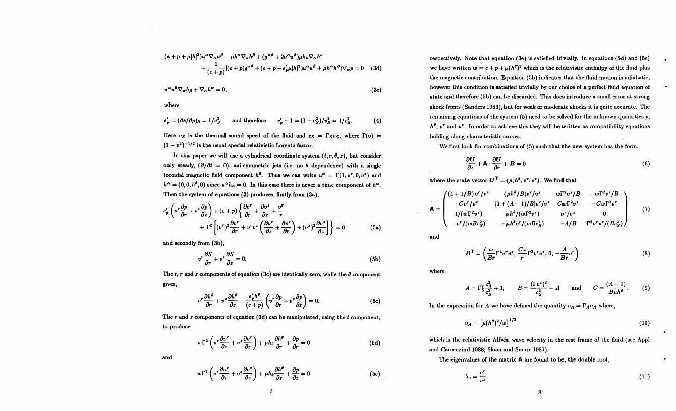
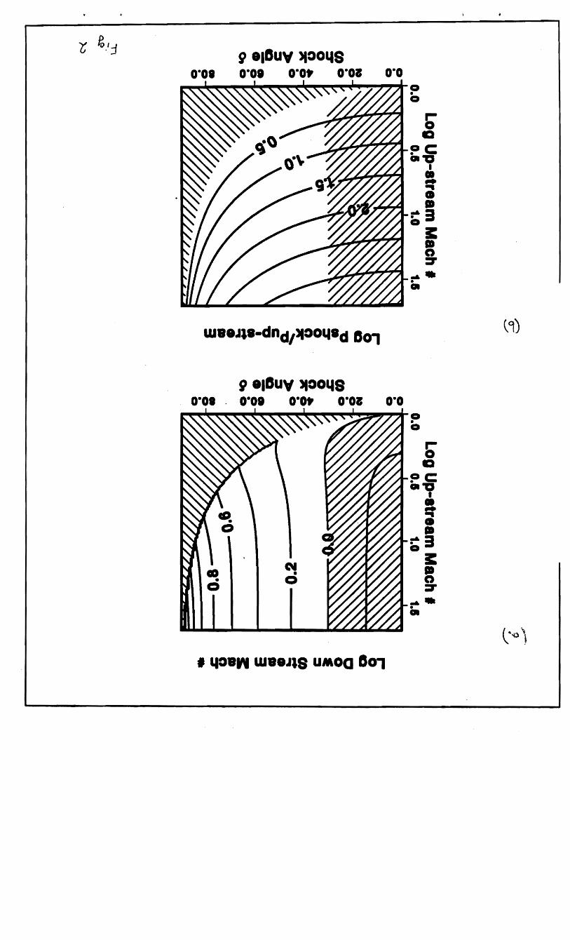

z
STXfl (q)
-z
(9)
(c)
z
-
(d)
r
z
shock path r
Pressure
P jet
P ext
r jet
B
H max
r
r ext
r jet
radius r radius jet
rpatch
radiusrJet
~~ pound
bull bull
o
-r--------------------------------------------------------------------~
~
I bull
t~_~-__-_bull
IG 0 bull
bull ~ ~~ ~ shyI ~~ I -0
c
I ~ -I _- 1 I ~ as bull ~ I I I I bull I ~ ~ I I~ middot1 I
bull-gt 0 0 II I 1 ~
II I I I - I - ICD t~ I I bull I I fC III bull I bull I I
IGbull0bull
o 9-~----------------------------------------------------------------~
00 500 1000 1500 2000 Z-Axis
bull
bull
L j
81XV shyomiddotoo~ 0middot08 0middot08
~--------------------------------------------------------~----------~~
~ ~
t1 riJ
Vmiddot
f v
- - V
~ ~ I Vj
Z
o
It=raquoC01 bullbullbull bullC0bull 0
0 I
0 gt)Ie01 -
bull
81XV - Z omiddotoo~
0middot08
0middot08 OmiddotOt
21 o
~
a
bullc
o shy
c
~----------------------~~------------------------~~ (~)N
obull0---------------------------_______________________ w
obull a~--------~--------~--------_--------_------~
00 200 400 800 800 1000 Z-Axis
-~-fi c ( to f )h~ 7 J
J
0
~bull
~
1 ~
I s ~
-51 tJi ~
~
8 ~JJ
(q)
______
bull bull10bull
10 bull
0
s 01bull
-a ata
10bull
10bull
bullbullbullbullbullbull bullbull bull bullbullbull
bullbullbullbullbullbullbullbullbullbullbull
bullbull --shy - fIII-shy shy~ __-shy ~ --- ~ ~ -shy
~ fill - bull bullbullbullbullbull
~~ bull bullbullbullbullbullbullbullbull bull bullbullbullbullbull~ ~
r
_----
O~----------------~~--------~--------~--------~---------400 100 1000 1100 1000 1100 3000
Z-Axis
o-
bull 0 0 bullgtC -c
c
bull0 0 bulls bull It bullbullbull aC
9 obull
~ -bullbull - bull
-shy-
- - ~-~~ -shy0iIII-__
~----------------~~--------~--------~--------~---------4bull 00 100 1000 1100 1000 1100 3000 Z-Axis
I
PUJT 1 152825 nut 7 MY 1992 middotttorh Dubl lAverJ or Tnoe 01SSPlft 110
r--shy ~ ~
Log H on Boundary Proper Mach on Axis -20 -11 -10 -01 00~I I
010shy
1
bullo
j I0_ obull I o
I
i
N
~ _0
shybull
N0_ Io
i zbullo
bull g cUo - Ii I I-Sgt
(-0 ~
g amp
-- - bullo obullo
01 10 00 200 400 800 o 1 s 1I~) I bullo
~
01 obullo
o obullo
N I -~bull ~ l
I
N o bull obull o
I
i Ii
bull I Ii~ f Imiddot o
bull
(a) (b) (c)
jiJ 10
bullbullbullbullbullbullbullbullbullbullbullbullbull
1
81XV - Z OmiddotOOS OmiddotOIL
bullr-------------------------------~--------~--------------------i_~o
sshybull a bull ~ o ~
CD - -~ ~~
i ~ bullbullbullbull l bullbullbullc - tI - ~ ~ - CD -- ~ ~ ~ - bull ~ -WI _ - ~ ~ bull o
-A _Imiddot ~ bull bull bullbull - ~ ~ o I ~ obull - -
~ ~ gtshy shy bull
)C
2 ~
~------------------------------------------~s (9)
0middot00middot0010middot008
bullP-------------------~--------------------------------------Oell
bull 0
- 7middot
D1 _ _ bullr-
bullbullbullbullbullbullbullbull - bullbullbullbull bullbullbull bullabullbull bullbull 0 bullbullbullbullbullbullbullbullbull bull 0- ~ -- -c~-------- ~ - ~ bull bullell ----------- - bullbull 0
bullbullbullbullbullbullbullbullbullbullbullbullbullbull
bullbullbullbull CDe-
Nbull0
~------------------------------------------------~c ~~)
obullo~----------------____________________________________~ GO
-bull)(-lt0Co omiddotbull c ~ ~ - -
~ ~ - t- bull - -
l ~
bull bull
~ -I -
~ -- - ~ imiddot~ - ~o e
CD~
~
~ - l ~ -- -- l - l ~ ~e shy
__ 11 _bull
Q fI_ ~ ~
o o~______bull
00
(rA) o
C
~~______~______~~______~______~________~
800 1000 1800 2000 2800 8000 Z-Axis
- p~----------------------------------------------------~ c fi bull-t0
-I shy shy 0
C
bullbullbullbullbullbullbull1bullbullbullbullbullbullbulli bullbullbullbullbullbullbullbullbullbull 1
bullbull t bullbullbullbullbullbullbullbullbullbull
II bullbullbullbullbullbullbullbullbullbullbullbull
~
I i It --shyf -shyPI 0 bull 8 8
bull 00 800 1000 1800 2000 2800 8000 Z-Axis
I I ( t()v- )~ a
c
61 ~Ij
(~)(0) (q)

bull bull
o
-r--------------------------------------------------------------------~
~
I bull
t~_~-__-_bull
IG 0 bull
bull ~ ~~ ~ shyI ~~ I -0
c
I ~ -I _- 1 I ~ as bull ~ I I I I bull I ~ ~ I I~ middot1 I
bull-gt 0 0 II I 1 ~
II I I I - I - ICD t~ I I bull I I fC III bull I bull I I
IGbull0bull
o 9-~----------------------------------------------------------------~
00 500 1000 1500 2000 Z-Axis
bull
bull
L j
81XV shyomiddotoo~ 0middot08 0middot08
~--------------------------------------------------------~----------~~
~ ~
t1 riJ
Vmiddot
f v
- - V
~ ~ I Vj
Z
o
It=raquoC01 bullbullbull bullC0bull 0
0 I
0 gt)Ie01 -
bull
81XV - Z omiddotoo~
0middot08
0middot08 OmiddotOt
21 o
~
a
bullc
o shy
c
~----------------------~~------------------------~~ (~)N
obull0---------------------------_______________________ w
obull a~--------~--------~--------_--------_------~
00 200 400 800 800 1000 Z-Axis
-~-fi c ( to f )h~ 7 J
J
0
~bull
~
1 ~
I s ~
-51 tJi ~
~
8 ~JJ
(q)
______
bull bull10bull
10 bull
0
s 01bull
-a ata
10bull
10bull
bullbullbullbullbullbull bullbull bull bullbullbull
bullbullbullbullbullbullbullbullbullbullbull
bullbull --shy - fIII-shy shy~ __-shy ~ --- ~ ~ -shy
~ fill - bull bullbullbullbullbull
~~ bull bullbullbullbullbullbullbullbull bull bullbullbullbullbull~ ~
r
_----
O~----------------~~--------~--------~--------~---------400 100 1000 1100 1000 1100 3000
Z-Axis
o-
bull 0 0 bullgtC -c
c
bull0 0 bulls bull It bullbullbull aC
9 obull
~ -bullbull - bull
-shy-
- - ~-~~ -shy0iIII-__
~----------------~~--------~--------~--------~---------4bull 00 100 1000 1100 1000 1100 3000 Z-Axis
I
PUJT 1 152825 nut 7 MY 1992 middotttorh Dubl lAverJ or Tnoe 01SSPlft 110
r--shy ~ ~
Log H on Boundary Proper Mach on Axis -20 -11 -10 -01 00~I I
010shy
1
bullo
j I0_ obull I o
I
i
N
~ _0
shybull
N0_ Io
i zbullo
bull g cUo - Ii I I-Sgt
(-0 ~
g amp
-- - bullo obullo
01 10 00 200 400 800 o 1 s 1I~) I bullo
~
01 obullo
o obullo
N I -~bull ~ l
I
N o bull obull o
I
i Ii
bull I Ii~ f Imiddot o
bull
(a) (b) (c)
jiJ 10
bullbullbullbullbullbullbullbullbullbullbullbullbull
1
81XV - Z OmiddotOOS OmiddotOIL
bullr-------------------------------~--------~--------------------i_~o
sshybull a bull ~ o ~
CD - -~ ~~
i ~ bullbullbullbull l bullbullbullc - tI - ~ ~ - CD -- ~ ~ ~ - bull ~ -WI _ - ~ ~ bull o
-A _Imiddot ~ bull bull bullbull - ~ ~ o I ~ obull - -
~ ~ gtshy shy bull
)C
2 ~
~------------------------------------------~s (9)
0middot00middot0010middot008
bullP-------------------~--------------------------------------Oell
bull 0
- 7middot
D1 _ _ bullr-
bullbullbullbullbullbullbullbull - bullbullbullbull bullbullbull bullabullbull bullbull 0 bullbullbullbullbullbullbullbullbull bull 0- ~ -- -c~-------- ~ - ~ bull bullell ----------- - bullbull 0
bullbullbullbullbullbullbullbullbullbullbullbullbullbull
bullbullbullbull CDe-
Nbull0
~------------------------------------------------~c ~~)
obullo~----------------____________________________________~ GO
-bull)(-lt0Co omiddotbull c ~ ~ - -
~ ~ - t- bull - -
l ~
bull bull
~ -I -
~ -- - ~ imiddot~ - ~o e
CD~
~
~ - l ~ -- -- l - l ~ ~e shy
__ 11 _bull
Q fI_ ~ ~
o o~______bull
00
(rA) o
C
~~______~______~~______~______~________~
800 1000 1800 2000 2800 8000 Z-Axis
- p~----------------------------------------------------~ c fi bull-t0
-I shy shy 0
C
bullbullbullbullbullbullbull1bullbullbullbullbullbullbulli bullbullbullbullbullbullbullbullbullbull 1
bullbull t bullbullbullbullbullbullbullbullbullbull
II bullbullbullbullbullbullbullbullbullbullbullbull
~
I i It --shyf -shyPI 0 bull 8 8
bull 00 800 1000 1800 2000 2800 8000 Z-Axis
I I ( t()v- )~ a
c
61 ~Ij
(~)(0) (q)
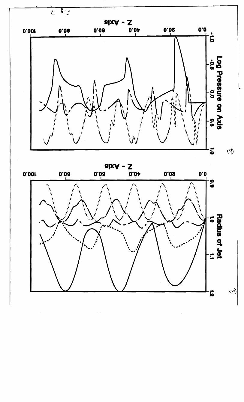
bull
bull
L j
81XV shyomiddotoo~ 0middot08 0middot08
~--------------------------------------------------------~----------~~
~ ~
t1 riJ
Vmiddot
f v
- - V
~ ~ I Vj
Z
o
It=raquoC01 bullbullbull bullC0bull 0
0 I
0 gt)Ie01 -
bull
81XV - Z omiddotoo~
0middot08
0middot08 OmiddotOt
21 o
~
a
bullc
o shy
c
~----------------------~~------------------------~~ (~)N
obull0---------------------------_______________________ w
obull a~--------~--------~--------_--------_------~
00 200 400 800 800 1000 Z-Axis
-~-fi c ( to f )h~ 7 J
J
0
~bull
~
1 ~
I s ~
-51 tJi ~
~
8 ~JJ
(q)
______
bull bull10bull
10 bull
0
s 01bull
-a ata
10bull
10bull
bullbullbullbullbullbull bullbull bull bullbullbull
bullbullbullbullbullbullbullbullbullbullbull
bullbull --shy - fIII-shy shy~ __-shy ~ --- ~ ~ -shy
~ fill - bull bullbullbullbullbull
~~ bull bullbullbullbullbullbullbullbull bull bullbullbullbullbull~ ~
r
_----
O~----------------~~--------~--------~--------~---------400 100 1000 1100 1000 1100 3000
Z-Axis
o-
bull 0 0 bullgtC -c
c
bull0 0 bulls bull It bullbullbull aC
9 obull
~ -bullbull - bull
-shy-
- - ~-~~ -shy0iIII-__
~----------------~~--------~--------~--------~---------4bull 00 100 1000 1100 1000 1100 3000 Z-Axis
I
PUJT 1 152825 nut 7 MY 1992 middotttorh Dubl lAverJ or Tnoe 01SSPlft 110
r--shy ~ ~
Log H on Boundary Proper Mach on Axis -20 -11 -10 -01 00~I I
010shy
1
bullo
j I0_ obull I o
I
i
N
~ _0
shybull
N0_ Io
i zbullo
bull g cUo - Ii I I-Sgt
(-0 ~
g amp
-- - bullo obullo
01 10 00 200 400 800 o 1 s 1I~) I bullo
~
01 obullo
o obullo
N I -~bull ~ l
I
N o bull obull o
I
i Ii
bull I Ii~ f Imiddot o
bull
(a) (b) (c)
jiJ 10
bullbullbullbullbullbullbullbullbullbullbullbullbull
1
81XV - Z OmiddotOOS OmiddotOIL
bullr-------------------------------~--------~--------------------i_~o
sshybull a bull ~ o ~
CD - -~ ~~
i ~ bullbullbullbull l bullbullbullc - tI - ~ ~ - CD -- ~ ~ ~ - bull ~ -WI _ - ~ ~ bull o
-A _Imiddot ~ bull bull bullbull - ~ ~ o I ~ obull - -
~ ~ gtshy shy bull
)C
2 ~
~------------------------------------------~s (9)
0middot00middot0010middot008
bullP-------------------~--------------------------------------Oell
bull 0
- 7middot
D1 _ _ bullr-
bullbullbullbullbullbullbullbull - bullbullbullbull bullbullbull bullabullbull bullbull 0 bullbullbullbullbullbullbullbullbull bull 0- ~ -- -c~-------- ~ - ~ bull bullell ----------- - bullbull 0
bullbullbullbullbullbullbullbullbullbullbullbullbullbull
bullbullbullbull CDe-
Nbull0
~------------------------------------------------~c ~~)
obullo~----------------____________________________________~ GO
-bull)(-lt0Co omiddotbull c ~ ~ - -
~ ~ - t- bull - -
l ~
bull bull
~ -I -
~ -- - ~ imiddot~ - ~o e
CD~
~
~ - l ~ -- -- l - l ~ ~e shy
__ 11 _bull
Q fI_ ~ ~
o o~______bull
00
(rA) o
C
~~______~______~~______~______~________~
800 1000 1800 2000 2800 8000 Z-Axis
- p~----------------------------------------------------~ c fi bull-t0
-I shy shy 0
C
bullbullbullbullbullbullbull1bullbullbullbullbullbullbulli bullbullbullbullbullbullbullbullbullbull 1
bullbull t bullbullbullbullbullbullbullbullbullbull
II bullbullbullbullbullbullbullbullbullbullbullbull
~
I i It --shyf -shyPI 0 bull 8 8
bull 00 800 1000 1800 2000 2800 8000 Z-Axis
I I ( t()v- )~ a
c
61 ~Ij
(~)(0) (q)
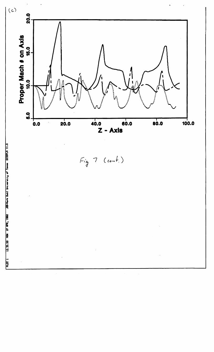
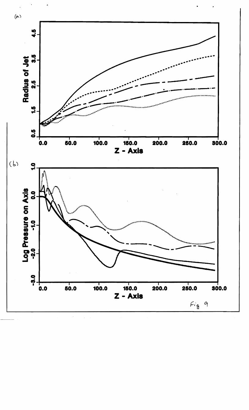

I
PUJT 1 152825 nut 7 MY 1992 middotttorh Dubl lAverJ or Tnoe 01SSPlft 110
r--shy ~ ~
Log H on Boundary Proper Mach on Axis -20 -11 -10 -01 00~I I
010shy
1
bullo
j I0_ obull I o
I
i
N
~ _0
shybull
N0_ Io
i zbullo
bull g cUo - Ii I I-Sgt
(-0 ~
g amp
-- - bullo obullo
01 10 00 200 400 800 o 1 s 1I~) I bullo
~
01 obullo
o obullo
N I -~bull ~ l
I
N o bull obull o
I
i Ii
bull I Ii~ f Imiddot o
bull
(a) (b) (c)
jiJ 10
bullbullbullbullbullbullbullbullbullbullbullbullbull
1
81XV - Z OmiddotOOS OmiddotOIL
bullr-------------------------------~--------~--------------------i_~o
sshybull a bull ~ o ~
CD - -~ ~~
i ~ bullbullbullbull l bullbullbullc - tI - ~ ~ - CD -- ~ ~ ~ - bull ~ -WI _ - ~ ~ bull o
-A _Imiddot ~ bull bull bullbull - ~ ~ o I ~ obull - -
~ ~ gtshy shy bull
)C
2 ~
~------------------------------------------~s (9)
0middot00middot0010middot008
bullP-------------------~--------------------------------------Oell
bull 0
- 7middot
D1 _ _ bullr-
bullbullbullbullbullbullbullbull - bullbullbullbull bullbullbull bullabullbull bullbull 0 bullbullbullbullbullbullbullbullbull bull 0- ~ -- -c~-------- ~ - ~ bull bullell ----------- - bullbull 0
bullbullbullbullbullbullbullbullbullbullbullbullbullbull
bullbullbullbull CDe-
Nbull0
~------------------------------------------------~c ~~)
obullo~----------------____________________________________~ GO
-bull)(-lt0Co omiddotbull c ~ ~ - -
~ ~ - t- bull - -
l ~
bull bull
~ -I -
~ -- - ~ imiddot~ - ~o e
CD~
~
~ - l ~ -- -- l - l ~ ~e shy
__ 11 _bull
Q fI_ ~ ~
o o~______bull
00
(rA) o
C
~~______~______~~______~______~________~
800 1000 1800 2000 2800 8000 Z-Axis
- p~----------------------------------------------------~ c fi bull-t0
-I shy shy 0
C
bullbullbullbullbullbullbull1bullbullbullbullbullbullbulli bullbullbullbullbullbullbullbullbullbull 1
bullbull t bullbullbullbullbullbullbullbullbullbull
II bullbullbullbullbullbullbullbullbullbullbullbull
~
I i It --shyf -shyPI 0 bull 8 8
bull 00 800 1000 1800 2000 2800 8000 Z-Axis
I I ( t()v- )~ a
c
61 ~Ij
(~)(0) (q)

c
61 ~Ij
(~)(0) (q)