Master project Artificial Intelligence:Investigating consonant inventories with acoustic and

articulatory models

Jan-Willem van Leussen, 0240184

University of AmsterdamSeptember 30, 2009

Examination comittee:prof. dr. P. Boersma

prof. dr. ir. R. Scha (chair)dr. M. van Someren (supervisor)

dr. D. Weenink (supervisor)

Abstract

The basic inventory of sounds (phonemes) used to encode speech varies considerably betweenlanguages. Nevertheless these inventories show an unmistakable preference for certain phonemesand phoneme configurations. It has oten been remarked that phonemic systems seem to strikesome balance between maximal perceptual distinctiveness and minimal speaker effort. Computermodels formalizing these principles have yielded phonetically quite accurate results for vowelconfigurations. This thesis describes a computational model that attempts to apply these sameprinciples to consonant phonemes, which are much more complex than vowels in articulatoryand acoustic terms.

The model makes use of an articulatory synthesizer to generate speech sounds and usesdynamic time warping (DTW) to judge perceptual similarity between these sounds. DTW isalso used to compare the resulting phonemes to those found in natural languages.

Results indicate that the model is able to arrive at a set of perceptually distinct consonantphonemes. However, the effort minimization parameter used in the model is not shown toresult in more common phonemes. I argue that the model may be a useful means of researchingphonological universals in consonant inventories but needs to be improved in several ways, whichare discussed at the end of the paper.

Contents

1 Introduction 41.1 Phonological patterns . . . . . . . . . . . . . . . . . . . . . . . . . . . . . . . . . 41.2 Innatism versus emergentism . . . . . . . . . . . . . . . . . . . . . . . . . . . . . 51.3 Computer models of language and speech evolution . . . . . . . . . . . . . . . . . 61.4 Modeling consonant inventories . . . . . . . . . . . . . . . . . . . . . . . . . . . . 8

2 Approach 102.1 Articulatory synthesis . . . . . . . . . . . . . . . . . . . . . . . . . . . . . . . . . 10

2.1.1 The articulatory model of Boersma (1998) . . . . . . . . . . . . . . . . . . 112.1.2 Constraining Boersma’s model to explore consonant space . . . . . . . . . 12

2.2 Creating a cost function for consonants . . . . . . . . . . . . . . . . . . . . . . . 142.2.1 Defining perceptual distinctiveness . . . . . . . . . . . . . . . . . . . . . . 162.2.2 Measuring perceptual distance with DTW and MFCCs . . . . . . . . . . 172.2.3 Defining articulatory effort . . . . . . . . . . . . . . . . . . . . . . . . . . 182.2.4 Combining effort and distinctiveness into a cost function . . . . . . . . . . 20

3 Search method 223.1 Searching a complex landscape . . . . . . . . . . . . . . . . . . . . . . . . . . . . 22

3.1.1 Overview . . . . . . . . . . . . . . . . . . . . . . . . . . . . . . . . . . . . 223.1.2 Initialization . . . . . . . . . . . . . . . . . . . . . . . . . . . . . . . . . . 233.1.3 Mutations . . . . . . . . . . . . . . . . . . . . . . . . . . . . . . . . . . . . 24

3.2 Summary . . . . . . . . . . . . . . . . . . . . . . . . . . . . . . . . . . . . . . . . 24

4 Evaluation method 274.1 Natural language data . . . . . . . . . . . . . . . . . . . . . . . . . . . . . . . . . 274.2 From auditory/articulatory data to phonemic classification . . . . . . . . . . . . 27

4.2.1 Incorporating articulatory features . . . . . . . . . . . . . . . . . . . . . . 284.3 Phoneme frequency as a naturalness metric . . . . . . . . . . . . . . . . . . . . . 294.4 Hypotheses . . . . . . . . . . . . . . . . . . . . . . . . . . . . . . . . . . . . . . . 32

4.4.1 The size principle . . . . . . . . . . . . . . . . . . . . . . . . . . . . . . . . 324.4.2 Balancing maximal distinctiveness and minimal effort . . . . . . . . . . . 32

5 Results 335.1 Qualitative analysis of results . . . . . . . . . . . . . . . . . . . . . . . . . . . . . 335.2 Quantitative analysis of results . . . . . . . . . . . . . . . . . . . . . . . . . . . . 34

5.2.1 Overview . . . . . . . . . . . . . . . . . . . . . . . . . . . . . . . . . . . . 355.2.2 Results for individual phonemes . . . . . . . . . . . . . . . . . . . . . . . 355.2.3 Effect of effort cost weight on naturalness . . . . . . . . . . . . . . . . . . 375.2.4 Effect of inventory size on naturalness . . . . . . . . . . . . . . . . . . . . 37

1

6 Conclusion and discussion 396.1 Summary and analysis of results . . . . . . . . . . . . . . . . . . . . . . . . . . . 396.2 Future work . . . . . . . . . . . . . . . . . . . . . . . . . . . . . . . . . . . . . . . 40

6.2.1 Improving the optimization model . . . . . . . . . . . . . . . . . . . . . . 406.2.2 Towards a non-teleological, speaker-oriented model . . . . . . . . . . . . . 41

7 Acknowledgements 42

List of Figures

1.1 Plot of relative frequency versus frequency ranking of UPSID segments . . . . . . 41.2 Maximizing F1/F2 distance in the vowel triangle . . . . . . . . . . . . . . . . . . 71.3 Relative frequencies of the 15 most frequent consonant phonemes in UPSID . . . 71.4 Schematic representation of constraints on consonant inventories . . . . . . . . . 9

2.1 Representation of the vocal tract in Boersma’s model . . . . . . . . . . . . . . . . 112.2 Synthesis example: /@B@/ . . . . . . . . . . . . . . . . . . . . . . . . . . . . . . . 132.3 Comparison of natural and synthesized nasal consonant . . . . . . . . . . . . . . 142.4 Overview of muscle parameters used in the model . . . . . . . . . . . . . . . . . . 142.5 Schematic representation of variation allowed in the articulatory model . . . . . . 162.6 Illustration of dynamic time warping of MFCC pairs . . . . . . . . . . . . . . . . 182.7 Scatterplot of DTW distances between 60 phonemes in an /a a/ context . . . . . 192.8 Schematic summary of cost function . . . . . . . . . . . . . . . . . . . . . . . . . 21

3.1 Effect of raising muscle activity on perceptual distance . . . . . . . . . . . . . . . 233.2 Example DTW distance matrix . . . . . . . . . . . . . . . . . . . . . . . . . . . . 24

4.1 Scatterplot of DTW distances between template segments . . . . . . . . . . . . . 29

5.1 Example of a 5-segment inventory after optimization . . . . . . . . . . . . . . . . 335.2 Synthetic vocal tract during /Q/-like articulation . . . . . . . . . . . . . . . . . . 345.3 Development of DTW distance between segments in a simulation run . . . . . . . 355.4 Frequencies of phoneme labels emerging from the simulations . . . . . . . . . . . 365.5 Effect of varying effort cost . . . . . . . . . . . . . . . . . . . . . . . . . . . . . . 375.6 Effect of inventory size on naturalness . . . . . . . . . . . . . . . . . . . . . . . . 38

These figures were drawn in Praat (Boersma and Weenink 2009), with the following excep-tions:

• Figures 1.1, 1.3, 3.1, 5.4, 5.5 and 5.6 were created in OpenOffice.org Calc.

• Figures 1.2 (adapted from Liljencrants and Lindblom 1972), 1.4 (adapted from Lindblom and Maddieson1988), 2.1 (adapted from Boersma 1998) and 2.8 were created in the vector graphics editorInkscape.

2

List of Tables

2.1 List of muscle parameters used in the model of Boersma (1998) . . . . . . . . . . 152.2 Displacement values for muscles in the model . . . . . . . . . . . . . . . . . . . . 20

4.1 Overview of the 18 consonant labels assigned to model output . . . . . . . . . . . 284.2 Frequency scores for phoneme labels . . . . . . . . . . . . . . . . . . . . . . . . . 31

5.1 Overview of simulation runs . . . . . . . . . . . . . . . . . . . . . . . . . . . . . . 365.2 p-values of t-test results comparing the effect of effort cost . . . . . . . . . . . . . 37

3

Chapter 1

Introduction

1.1 Phonological patterns

Natural languages show remarkable variety in the number of different sounds (phonemes) thatare used as units in speech. The conventional method of transcribing speech sounds, the Inter-national Phonetic Alphabet IPA (1999), uses 107 distinct symbols to encode speech sounds, andalso includes more than 50 diacritics to indicate slight specifications on this basic set of symbols.Indeed, some languages distinguish between a large number of these sounds. For instance, theEnglish phoneme inventory distinguishes approximately 45 phonemes, of which about 20 arevowels and about 25 are consonants (Roach 2000). The Khoisan language !Xoo has the largestknown phoneme inventory, with at least 58 consonants and 31 vowels (Traill 1985). Smallerphoneme inventories are more common, however; the average seems to lie somewhere between20 and 40 (Clark et al. 2006).

Figure 1.1: Plot of relative frequency (in percent, vertical axis) versus frequency ranking (absolute,horizontal axis) of UPSID phoneme segments

4

Despite this variety, the distribution of phonemes among different languages is far from ar-bitrary. The UPSID (UCLA Phonological Segment Inventory Database, Maddieson and Disner1984), a statistical survey of the phonological inventories of 451 languages, shows that the con-sonants /m/, /k/, /p/ and /j/ and the vowels /a/, /i/ and /u/ all occur in over 80% of thelanguages in the database. On the other hand the front rounded vowel /y/ occurs in only about5% of the surveyed languages, and many consonant segments are even rarer (like the click conso-nants of the aforementioned !Xoo, some of which are only attested in that language). Generallythe segments in the database show a Zipfian distribution (Zipf 1949), where a small number ofphonemes are extremely common crosslinguistically, whereas a large number of phonemes occuronly very rarely (Figure 1.1).

Looking beyond the distributions of individual phonemes, there are are also common pat-terns to be found in the organisation of sounds within phoneme inventories. Rarer (marked)phonemes tend to occur more frequently in larger inventories, and the appearance of a markedphoneme in an inventory often implies the presence of a similar unmarked phoneme. For in-stance, the presence of the marked close rounded front vowel /y/ in a phoneme inventory impliesthat this language also has its unmarked counterpart, the close unrounded front vowel /i/. Ten-dencies of this sort are called phonological universals, and occur across languages that are notprovably related.

Languages and their phoneme inventories are not static entities; as they are transmitted fromgeneration to generation they are subject to change. A well-documented historical exampleis the branching of the Romance language family: the 10-vowel inventory of Classical Latin(Allen 1989) grew to 17 vowels in modern French and shrank to 5 vowels in modern Spanish(Battye et al. 2000). From a diachronic perspective, saying that certain phonological patternsare more common than others can be rephrased as stating that certain phonological states aremore stable or attractive than others over time. However, there is considerable controversy anddebate over the mechanisms behind this stability. The next section examines these differentviewpoints in more detail.

1.2 Innatism versus emergentism

Broadly speaking, explanations for phonological tendencies or universals come in two forms.The first type of hypothesis argues that preferences for certain phonological patterns are to someextent innate, that is to say, hard-wired into the human capacity for language learning. Thesecond type of hypothesis views phonological patterns as emergent : they arise as a consequenceof phonetic properties of the phonemes themselves and the way they are transmitted. Moreton(2008) calls the two types of hypotheses analytical bias and channel bias respectively, andstresses that they need not be mutually exclusive.

Theories of innate phonological bias are usually connected to Chomsky (1965)’s theory ofGenerative Grammar (which primarily concerns syntax) and were made explicit for phonologyin Chomsky and Halle (1968). Generative views on phonology often describe phonemes in termsof basic distinctive features. Each phoneme can be described in terms of a unique combinationof these features, and sets of features can describe classes of phonemes which undergo somephonological process. Innatist approaches to phonological typology state that features do notmerely serve a descriptive purpose: rather, the crosslinguistic predisposition toward certainfeature combinations and classes suggest that there is a cognitive basis to the features.

There has also been some psychological research supporting an innate bias. For example,Caramazza et al. (2000) found evidence from two aphasics that consonants and vowels areprocessed separately, suggesting a cognitive basis for the universal phonological distinctionbetween vowels and consonants. Indications of neurological correlates for more fine-grained

5

phonemic distinctions have also been found (e.g. Eulitz and Lahiri 2004).Proponents of emergentist theories (sometimes also called substance-based theories) point

out that many aspects of phonological typology seem to be governed by phonetic principles. Onesuch property is perceptual contrast : phonological inventories tend to organize sounds in such away that they are maximally auditorily distinct from one another. This is especially apparentin the organisation of vowel inventories. The UPSID shows that languages with three vowelsoverwhelmingly have the configuration (/a/, /i/, /u/) (Maddieson and Disner 1984). Thesethree vowels are maximally dispersed in terms of their first and second formant frequencies,which are considered the most important cues in vowel perception (Klein et al. 1970). Obviouslythere are benefits to such dispersion: it diminishes the probability of confusing one phonemefor another, making communication in a noisy environment more efficient.

This tendency towards maximal auditory dispersion seems to be counterbalanced by atendency toward maximizing articulatory efficiency (see e.g. ten Bosch 1991). According toBoersma and Hamann (2008), languages with only one phoneme on a given auditory contin-uum often place it in the center of this continuum, corresponding to an articulation whichrequires least effort. The Quantal Theory of Stevens (1972) explains phoneme distributions inboth articulatory and acoustic terms: it states that languages prefer phonemes which are robustto small variations in articulations.

As the long-term acquisition of spoken language is impossible to recreate in a laboratorysetting, direct empirical research into either hypothesis is not feasible. However, it can beargued that generally, emergentist explanations are more elegant: they refer to measurableproperties of speech production and perception. On the other hand explanations in terms ofinnateness often rely on postulating complex neurological structures, about which much remainsunknown and which can only be verified indirectly, at best. This means that explanationsviewing phonological patterns as emergent are preferable per Occam’s Razor; if a phonologicaluniversal has a plausible explanation in emergentist terms, this eliminates the need for a morecomplicated model of innate bias. The next section will focus on some computational researchon language and speech acquisition supporting an emergentist view.

1.3 Computer models of language and speech evolution

Over the last decades, computer modeling has gained popularity as a means of research intolanguage evolution. These models concern both the biological evolution of language (simulatingthe emergence of the language faculty in our hominid ancestors) and the cultural evolutionof language (simulating sound and language change). An example of the latter is the Iter-ated Learning Model (ILM) of Kirby and Hurford (2002). In this model, interaction betweenindividuals is modeled in a simple ‘protolanguage’. Even without pressuring for efficient com-munication, essential properties of natural language such as compositionality and recursivityemerge spontaneously in a population of simulated learners (Kirby 2001). This indicates thatlinguistic structure and regularity may emerge without any a priori innate preference for it.

In the field of phonetics and phonology, computational research into sound systems haslikewise indicated that many properties of sound systems are emergent. An pioneering study inthis respect was performed by Liljencrants and Lindblom (1972), who found that many commonvowel systems can be easily explained in terms of acoustic properties of the vowels themselves:by calculating for a given number of vowels a configuration that maximizes the distance betweenvowels in terms of their first and second formant, configurations closely resembling those foundin many languages emerged. (Figure 1.2). These results have more recently been refined bySchwartz et al. (1997).

6

3 4 5

Figure 1.2: Maximizing F1/F2 distance between 3, 4 and 5-vowel configurations, adapted fromLiljencrants and Lindblom (1972); the rightmost figure shows a plot of Dutch vowels for comparison(data from Pols et al. 1973), with the corner vowels /a/, /i/ and /u/ circled.

de Boer (2001) simulated the emergence of dispersed vowel systems in a population of simu-lated speakers (agents) without explicitly modeling a need for maximization of acoustic distance:rather, the agents strived toward minimizing communication errors, and realistic dispersionemerged in their shared language as a consequence. Oudeyer (2001) elaborated on these re-sults with a simulation that included a simple articulation model capable of producing syllablesconsisting of both consonants and vowels. Zuidema and de Boer (2009) showed, again throughan agent-based simulation, that phonemic coding (re-using different combinations of sounds)emerges as a better means of communication than a sound system consisting of only holis-tic signals. Sounds in this simulation were represented as trajectories on an abstract plane.van Leussen (2008) combined the model of de Boer (2001) with a model of phoneme dispersionby Boersma and Hamann (2008) based on Optimality Theory (Prince and Smolensky 1993) toshow how articulatory effort might be incorporated in an agent-based model of vowel dispersion.

Figure 1.3: Relative frequencies of the 15 most frequent consonant phonemes in UPSID. The mostfrequenct consonant, the bilabial nasal /m/, occurs in the inventories about 94% of the languages in thedatabase.

7

1.4 Modeling consonant inventories

While computer models into phonological patterns have yielded phonetically very accuratepredictions for vowel systems, modeling consonant inventories has remained more elusive. Sim-ulations involving consonants or consonant-vowel combinations often represent the space ofpossible phonemes abstractly (see e.g. Boersma 1989, Mielke 2005), or in terms of their phono-logical features. Using predefined categories or abstractions limits the explanatory power ofthese simulations, since the outcome is shaped by the phonological categories assigned to theinput. The reason for these abstractions must probably be sought in the difficulty of formalizingthe phonetic properties of consonants.

By their nature consonants are often more complex than vowels in terms of their articulation,acoustics, and the relation between these two. Vowels can be classified quite accurately in termsof just the first and second formant frequencies (or effective second formant frequency, see Bladon1983). Articulation of vowels is usually reduced to three dimensions: tongue height, tonguebackness, and lip rounding (for example de Boer 2001). Furthermore, there is a clear monotoniccorrelation between these articulatory dimensions and the first and second formant frequencies(Traunmuller 1981, Ladefoged 2005). On the other hand cues for consonant perception aremore numerous, harder to place on a continuum, and often depend on spectral transitions anddurations rather than static qualities (Delattre et al. 1955). Articulatory aspects of consonants,particularly manner of articulation, often do not form a clear continuum; and there is oftennot a monotonic relation between articulatory gestures and acoustic properties of the resultingsound the way there is for vowels.

Nevertheless, languages show a clear preference for a small subset of consonants out of thehundreds of distinct possible consonants sounds (see Figure 1.3). Emergentist explanationsof these tendencies in consonant inventories often state that the same principles that accountfor vowel typology apply to consonants. Figure 1.4, adapted from Lindblom and Maddieson(1988), ilustrates the tension between two of these principles mentioned earlier: maximizingperceptual distinctiveness and minimizing articulatory effort. ‘Phonetic space’ is representedas an amorphous blob, indicating the difficulty of defining the acoustics of consonant phonemeson any sort of numerical scale.

This paper presents a model for finding optimal consonant configurations under the afore-mentioned constraints on distinctiveness and effort. If these are indeed the main forces actingupon consonant inventories, the model should predict the clear preference for certain conso-nants above others found in natural language (Figure 1.3). Optimizing within consonant spacerequires the following ingredients:

1. A means of defining the articulatory borders of the phonetic space, and generating allpossible states within these borders;

2. A means of defining perceptual distance between points in this space;

3. A means of translating this perceptual distance and other properties of consonant inven-tories to parameters in a cost function, and a method to optimize this function.

4. A means of comparing the results of the optimization to natural language data, in orderto test the the relative importance of the cost parameters in the model.

This paper will attempt to show that all ingredients are within reach using existing tech-niques from speech synthesis, speech recognition, and artificial intelligence. By using an articu-latory synthesizer, articulatory properties of phonemes may be formalized, and the state spacecan automatically be constrained to the set of speech sounds that can be produced by human

8

beings - provided the synthesizer is realistic enough. Methods of defining perceptual distancebetween pairs of sounds have been studied extensively in automated speech recognition andrelated fields, and these same techniques can be used to interpret the results. Finally, findinga global optimum in a complex multidimensional landscape is at the heart of many problemsin AI. While these techniques have all been applied to research into speech sound patterns inearlier studies, I believe combining them in a single model of consonant typology has not beenattempted so far.

Phonetic

space

Neutral articulations

"Magnets" (perceptual distinctiveness)

"Rubber band" (articulatory simplification)

Figure 1.4: Schematic representation of the main phonetic forces acting upon consonant inventories,adapted from Lindblom and Maddieson (1988). Phonemes are magnetically pulled toward perceptuallydistinctive states, but at the same time rubber bands tie them toward neutral, less effortful articulations.

The paper is organised as follows: Chapter 2 provides more details on the different com-ponents of the model and explains some of the choices made, and Chapter 3 describes theimplementation of these components in an optimization algorithm. Chapter 4 explains how thesimulation outcomes may be evaluated against natural language data. Chapter 5 shows theoutcome of running simulations with the model using different optimization parameters. Therelevance of these results, and suggestions for future improvements on the model, are discussedin Chapter 6.

9

Chapter 2

Approach

2.1 Articulatory synthesis

Although mechanical emulation of the human speech apparatus has been attempted for cen-turies1, nowadays the term articulatory speech synthesis is normally taken to mean softwaremodels. Articulatory synthesizers produce sound by modeling the movement of air through thevocal tract, which is usually represented as a series of interconnected tubes. Manipulating thewidth of the tubes at various points, either directly or through parameters representing themuscles controlling certain articulators in the vocal tract, affects the resulting waveforms. Anearly model that synthesized vowels was made by Kelly and Lochbaum (1962). More sophisti-cated models capable of synthesizing consonants and consonant-vowel combinations have alsobeen developed (eg. Mermelstein 1973, Maeda 1982); and more recently, a three-dimensionalvocal tract model, based on articulatory data from MRI studies, has been developed by Birkholz(2005).

Articulatory synthesis is theoretically an attractive model for text-to-speech (TTS) systems,since perceived speaker attributes such as age and gender can be varied simply by changing therelevant parameters controlling the simulated vocal tract (Shadle and Damper 2001). Neverthe-less, over the years commercial TTS systems have moved away from articulatory synthesis to-ward concatenative synthesis based on pre-recorded segments (Klatt 1987, Jurafsky and Martin2008). The acoustical calculations involved in realistic articulatory synthesis are still too de-manding to perform in real-time; and despite the advances described in the previous paragraph,natural-sounding voice quality in running speech remains hard to attain.

However, articulatory synthesis has seen extensive use as a tool in phonetic and phonologicalresearch. For instance, modifications of human articulatory models have been used to investigatethe vocal abilities of apes and monkeys (de Boer 2008) and Neanderthals (Boe et al. 2002).The model of Birkholz (2005) has been used to investigate the effect of larynx height on vowelproduction by Lasarcyk (2007).

For the research into phonetic properties of consonant inventories described in this paper, Ihave decided to use the articulatory synthesizer of Boersma (1998). The choice for this modelwas primarily based on the following:

• While the model is limited in its ability to synthesize vowels (Boersma, personal com-munication, May 2009), it is capable of synthesizing many different types of consonants,including ejectives, trills and clicks, making it well-suited for research into consonantinventories.

1An extensive overview of the history of speech synthesis is available at the website of Haskins Laboratories:http://www.haskins.yale.edu/featured/heads/heads.html

10

• Rather than vocal tract shapes or phonologically informed gestures, the model takes mus-cle activity as input, which can be directly related to the notion of articulatory effortmentioned in Chapter 1.2. This also means that the model is not biased toward certainphonemes a priori.

• A working and scriptable version of the model is available in the software package Praat(Boersma and Weenink 2009), which conveniently can also be used for phonetic analysisof the articulations and resulting waveforms.

2.1.1 The articulatory model of Boersma (1998)

This section will provide a short overview of Boersma’s model necessary to explain its role in thesimulations described in this paper, and also describes a number of limitations in its ability tosynthesize consonant sounds. For an exhaustive description of the model, including the physicalequations used to model airflow and movement of the vocal tract walls, the reader is referredto Boersma (1998).

A major difference between Boersma’s model and most other articulatory models is thatsource and filter (Fant 1970) are not independent components. Instead, the entire vocal appa-ratus is modelled as a series of interconnected tubes, starting at the lungs and radiating intothe atmosphere at the lips and nostrils. The vocal cords are also modelled in this manner.Springs are connected to the walls of these tubes, controlling their position and stiffness (seeFigure 2.1). A set of 29 muscles controls these springs; thus, the shape of the tract is ultimatelydetermined by the activities of each of these muscles. By varying the shape of the tract overtime while causing air to flow through it, speech sounds may be created.

Lungs Pharynx Lips

Figure 2.1: The vocal tract as represented in Boersma’s model. The position and elasticity of the walls arecontrolled by various muscles through springs, and by the flow of air through the tract. Neighbouringwalls are also connected by springs. Acoustic output is determined by the airflow radiating into theatmosphere at the lips (and at the nostrils; the nasal tract is not shown in this figure). Adapted fromBoersma (1998).

Utterances in the model are specified as a series of muscle activity targets on a timelinerunning from zero to a user-specified length. These targets represent muscle activity as avariable between zero (at rest) and one (fully contracted) 2. By default two targets are specified

2The activity parameters may actually also take on negative values. However, since these are not necessary toproduce realistic articulatory movements and represent an anatomical impossibility (muscles may only contractin one direction), the activity parameters are kept within the range of [0,1] in the model described herein.

11

for each muscle: zero activity at the start of the utterance, and zero activity at the end ofthe utterance. The amount of activity at a given point on the timeline is linearly interpolatedbetween target points. By setting a nonzero target for a muscle on a point on the timeline,contraction of this muscle is initiated, resulting in movement of the associated articulator.

As an example, creating a 0.5 second utterance that sounds like /@B@/ requires setting atleast four muscle parameters:

• To cause an outward movement of air, the air in the lungs must be compressed. This isdone by decreasing the Lungs parameter from 0.1 at 0 seconds to 0.0 at 30 ms.

• To make the vocal cords vibrate when air passes them, they must be tensed somewhat,but not completely (which would close them and prevent air from escaping). This is doneby setting the Interarytenoid parameter to 0.5 throughout the utterance.

• To make sure air only escapes through the mouth, the velum must be raised so thatthe nasal tract is closed off. This is done by setting the LevatorPalatini parameter to 1throughout the utterance.

• To create a transition from the vowel /@/ to the consonant /B/ and back again, the lipsmust be brought close together (but not closed) in the middle of the utterance. This isdone by setting the OrbicularisOris parameter to 0.7 between 200 and 300 ms. To makesure the vowel quality remains constant for an instant before and after articulation of theconsonant, this same parameter is kept at 0 between 0 and 100 ms and between 400 and500 ms.

Figure 2.2 illustrates the effect of superimposing these muscle gestures on a male-like vocaltract.

A variety of different consonant sounds can be synthesized in this manner; nevertheless,there are also sounds that cannot be synthesized convincingly with the articulatory model asset out in Boersma (1998). Most notably, I have not been able to synthesize natural soundingnasal consonants (/m/,/M/,/n/,/ n/,/ñ/,/N/ and / N/). Articulatory, nasal consonants are char-acterized by a complete closure somewhere in the oral cavity, so that all air flows out throughthe nose. Acoustically this results in a sound with clearly distinguishable formants, which arehowever much fainter than in vowels (Ladefoged 2005). While Boersma’s model does allow forthe modeling of these types of consonants by creating an oral closure and lowering the velum,the resulting sound cannot be said to resemble a nasal consonant (Figure 2.3).

The class of sibilant fricatives (/s/,/z/,/S/,/Z/,/ s/ and / z/) also cannot be synthesized well.This class of sounds is characterized by a high amount of noise in the upper region of the auditoryspectrum, which is caused by a jet of air directed against the upper teeth through a narrowconstriction between the tongue and the roof of the mouth. The aerodynamic calculationsrequired for modeling this process are not incorporated in the articulatory model (Boersma,personal communication, June 2009).

These limitations, which are intrinsic to the model, regrettably constrain the number ofspeech sounds that can be explored using Boersma’s model. Some of these limitations onlybecame apparent after significant time had already been invested in incorporating this articula-tory synthesizer into the model. The following section will explain some additional constraintswhich I imposed to prevent the search space from growing too large.

2.1.2 Constraining Boersma’s model to explore consonant space

Because input to Boersma’s model comes in the form of parameters specifying muscle activity,it is very well suited to computational exploration of the phonetic space available to humans

12

0 0.5-1

0

1Lungs

Time (s)0 0.5

-1

0

1LevatorPalatini

Time (s)0 0.5

-1

0

1Interarytenoid

Time (s)0 0.5

-1

0

1OrbicularisOris

Time (s)

@ B @

Time (s)0 0.5

0

5000

Fre

quen

cy (

Hz)

Fre

quen

cy (

Hz)

0 0.1 0.2 0.3 0.4 0.5

Figure 2.2: Synthesizing an /@B@/-like utterance in a male voice. The top graphs show the values of themuscle parameters over time; the middle figure shows an annotated oscillogram of the sound; the bottomfigure is a spectrogram of the sound.

in the production of consonant sounds. However, the realism of the model comes at a highcomputational cost: at the moment of writing, synthesis of a single 0.5 second utterance takesseveral seconds on a reasonably modern personal computer. Any search of articulatory spacewill therefore be severely bottlenecked by the synthesis component. Furthermore, since only asmall number of muscle movements will actually cause the airflow necessary to produce speech,a lot of search time may be wasted on finding articulations that result in any sound at all,rather than those that produce distinct consonants. To keep the time taken by the simulationswithin acceptable bounds, it was necessary to put some constraints on the articulations that aretried during search, both in terms of the muscle parameters used and in terms of their temporalspecification.

An important constraint is that of the 29 muscle parameters available in the model, I allowonly a subset of 14 to change during search. Specifically, only muscle parameters that controlthe tongue, mouth and oropharyngeal cavity can be changed. I will call this subset of musclesM. Table 2.1 and Figure 2.4 give an overview of the muscles used and their effect on vocaltract shape. The other muscles are not used in the articulations produced during search, withthe exception of the following parameters which are standard for each articulation:

• The Lungs parameter is set to 0.1 at 0 ms and to 0.0 at 30 ms to create air pressure inthe vocal tract.

• The InterArytenoid parameter is set to 0.5 throughout the utterance to create phonationwhen air passes the vocal folds.

• The LevatorPalatini parameter is set to 1.0 throughout the utterance, sealing off the nasal

13

Time (s)0 0.4682

0

5000

Fre

quen

cy (

Hz)

Time (s)0 0.46

0

5000

Fre

quen

cy (

Hz)

a m a a “m” a

Figure 2.3: A spectrogram of a real male speaker saying /ama/ (left) and of a synthesized male speakermaking /ama/-like articulatory movements in Boersma’s model (right). The fainter formants associatedwith nasal consonants are not reproduced faithfully in articulatory synthesis; the resulting utterancesounds more like /ala/.

tract.

Hyoglossus Styloglossus Genioglossus UpperTongue LowerTongue TransverseTongue VerticalTongue

Risorius OrbicularisOris TensorPalatini Masseter Mylohyoid LateralPterygoid Buccinator

Figure 2.4: Overview of muscle parameters that are changed during search, showing a sagittal cross-section of the vocal tract when the value of that parameter is 1. Note that some muscles do not showa change in tract shape, as they either control tenseness rather than position of a wall, or cause onlylateral movement.

A second important constraint is that I limit the time during which the activity of the musclescan vary. The consonant segments tried during search are embedded in an unchangeable /@ @/environment: that is, they are preceded and succeeded by the neutral vowel schwa, which isproduced by making the vocal cords vibrate while keeping the nasal tract closed and relaxing thetongue and mouth muscles. The choice of schwa should prevent the vowel context from exertingtoo large an influence on the consonants. To make sure the beginning and end of the producedutterances remain constant, the muscle parameters are fixed at zero during the vowel segments,and may only take on another value in the middle segment. During this middle segment theirvalue also remains fixed: movement of articulators only takes place during a transitory periodbetween the vowel and consonant segment (Figure 2.5). With these constraints, we can definethe activity of a muscle m from the set M using a single real-valued parameter am, and definea consonant segment c as a set of activity values {am1

, am2· · · amn

}, where n = |M|.

2.2 Creating a cost function for consonants

The articulatory model of Boersma, described in the previous section, is able to generate astate space for our model of consonant distribution. To optimize in this space, it is necessaryto find a cost function that reflects proposed optimal properties of consonants and consonantinventories. Two of these properties will be investigated in this paper: maximal perceptual

14

Table 2.1: List of muscle parameters in the articulatory model of Boersma (1998). Note that someof these muscles have overlapping functions, while others are antagonists of one another, i.e. pull thearticulators into opposite directions. Only a subset of these 29 muscles is explored in the optimizationmodel described in this paper. The rows shaded gray represent parameters for which the value is fixedduring search; the unshaded rows are the subset of musclesM that are explored in search.

Name of muscle (group) Function

Buccinator Tenses oral wallsLateralPterygoid Moves jaw horizontallyMylohyoid Lowers mandible, opening mouthMasseter Raises mandible, closing mouthTensorPalatini Lowers velumOrbicularisOris Purses lipsRisorius Spreads lipsVerticalTongue Makes tongue thinnerTransverseTongue Makes tongue thickerLowerTongue Lowers tongue tipUpperTongue Raises tongue tipGenioglossus Moves tongue forwardStyloglossus Moves tongue back and upwardsHyoglossus Moves tongue downwards

LevatorPalatini Raises velumSphincter Constricts pharynxUpperConstrictor Constricts upper part of pharynxMiddleConstrictor Constricts middle part of pharynxLowerConstrictor Constricts lower part of pharynxThyropharyngeus Constricts ventricular foldsSternohyoid Lowers larynxStylohyoid Raises larynxLateralCricoarytenoid Opens glottisPosteriorCricoarytenoid Closes glottisThyroarytenoid Relaxes vocal foldsVocalis Tenses vocal foldsCricothyroid Tenses vocal foldsInterarytenoid Adducts vocal foldsLungs Expands lungs

15

Mutable (consonant) segment

Transition segments

Fixed (vocalic) segments

Figure 2.5: A graph representing possible articulatory movement over time for the 14 muscles that areused in search. A single real-valued parameter between 0 and 1 represents the activity of a given muscleduring the middle (consonantal) segment. The activity will be 0 (relaxed) during the vowel segment,and movement from zero activity to the specified level of activity takes place in the transition segment.

contrast and minimal articulatory effort. The first is a property of consonant sets which canbe derived by comparing the waveforms of different utterances generated by the articulatorysynthesizer; the second is a property of consonants themselves, and can be derived directly fromthe muscle activity patterns which serve as input to the synthesizer.

2.2.1 Defining perceptual distinctiveness

Computational models of vowel sytems usually define perceptual distance using some weightedcombination of their first and second (and sometimes third and fourth) formant values, whichnumerous perception experiments have shown to be the primary cues for vowel perception.Cues for consonant perception are also to be found in the spectrum. For example, in languagesthat have a contrast between voiced and voiceless plosives, an important cue that determineswhether voicing is perceived is Voice Onset Time (VOT), the time elapsed between release of aplosive and the start of vocal cord vibration (Lisker and Abramson 1963). However this samecue plays no role in the perception of sibilant fricatives, which are primarily identified throughthe location of intensity peaks in the spectrum (Harris 1958). Cues for place of articulationare often found in formant transitions, making them dependent on the preceding and followingsegments. Clearly, combining these different types of cues into a single perceptual distancemetric is not as straightforward as it is for vowels.

The problem of defining a global measure of perceptual contrast is briefly considered byBoersma (1998). However, he ultimately dismisses the notion of a global contrast measure as”linguistically irrelevant”, since perceptual difference is known to depend heavily on the lan-guage(s) the hearer is proficient in; the language one is exposed to can determine the perceivedcontrast between two segments (e.g. Kazanina et al. 2006). This holds true when modelinglanguage at the level of the speaker, but as the model described in this paper concerns crosslin-guistic notions of optimal distance, a global distance metric is indeed relevant. Furthermore,the ubiquity of certain types of vowel systems mentioned in Maddieson and Disner (1984), and

16

research on perception of speech sounds by nonhuman animals (e.g. Kuhl 1981) indicate thatperceptual distance is at least partially grounded in common properties of mammalian hearing.

At this point it is instructive to take a look at best practices in the area of automatic speechrecognition. After all, speech recognition is also concerned with mapping an incoming speechsignal to a best fit among a set of stored signals. An effective metric of similarity betweensegments is therefore desirable for accurate recognition. The next section describes how onesuch measure, dynamic time warping on mel-frequency cepstral coefficients, can be used as aneffective method for computing perceptual distance between two consonant segments.

2.2.2 Measuring perceptual distance with DTW and MFCCs

Dynamic time warping (DTW) is an algorithm for measuring similarity between two signals orsequences, which is robust to variations in time and speed (speaking rate). Both signals aredivided into a number of frames, which contain vectors representing features or measurementsfrom that point in the signal. A matrix representing the distance between each frame of thefirst signal and each frame of the second signal may be computed according to some distancefunction defined on the feature vectors. The least costly path through this matrix may thenbe computed, for instance using the Viterbi algorithm (Viterbi 1967). The length of this pathrepresents the ‘warp’ or distance between the two signals. The accuracy of DTW as a distancemeasure can be improved by placing some constraints on the minimum and maximum slope ofthe path (Sakoe and Chiba 1978).

Perceptual features for comparing speech signals can be extracted by dividing the powerspectrum into a number of frequency bins and taking the power of the signal inside eachof these bins. Because human hearing is not organized along a linear scale, more accuratefeature vectors can be created by first transforming the sound signals to the psychoacous-tic Mel scale (Stevens and Volkmann 1940) using mel-frequency cepstral coefficients (MFCCs,Bridle and Brown 1974; Davis and Mermelstein 1980). MFCCs are a fairly effective metric forthe recognition of isolated segments (e.g. Sroka and Braida 2005) and are also used in the fieldof automatic music recognition and retrieval (Tzanetakis and Cook 2002). Employing DTW asa measure of perceptual distance between phonemes was inspired by Mielke (2005).

For this paper, I have used the MFCC and DTW implementations of Praat (Boersma and Weenink2009), using the standard settings for creating MFCCs from waveforms. Under these settings,the sound is divided into windowed frames of 15 ms, with a sampling period of 5 ms, and 12mel-frequency cepstral coefficients are calculated on these frames using the method described inDavis and Mermelstein (1980). Distances between frames can then be calculated as a weightedsum of three components:

1. euclidean distances between the cepstral coefficients

2. euclidean distance between the log energy (loudness) of frames

3. the regression coefficient of the cepstral coefficients over a number of subsequent frames

However, weights (2) and (3) were set to zero in the experiments described in this paper, asthey did not seem to have a positive effect on the effectiveness of the distance metric. Thereforethe mutual distance dij between two MFCC frames i and j is calculated with the formula

numCoefficients∑

k=1

(cik − cjk)2 (2.1)

where numCoefficients = 12 and cij is the jth coefficient of frame i. The optimal Viterbipath through the matrix of frame distances is then calculated, with the constraint that the first

17

and final frames of the two signals match, and that the path lie between two lines with slopes1

3and 3.Figure 2.6 shows DTW paths for comparisons of a male speaker saying /asa/, /apa/ and

/aza/. In terms of phonological features, the segment pair /s/-/p/ is more distant than thepair /s/-/z/; the first pair differs both in place of articulation (Alveolar vs Bilabial) andmanner of articulation (Fricative vs Plosive), the second pair only in voicing (Voiceless

vs Voiced). This is reflected by a shorter DTW path for the pair /asa/-aza/.

0

0.6556

0 0.488027211

DTW of /asa/ vs /apa/ (distance: 142.007)

0

0.6556

0 0.683673469

DTW of /asa/ vs /aza/ (distance: 86.813)

Figure 2.6: An illustration of dynamic time warping on two pairs of MFCCs. Left shows /asa/ (vertical)versus /apa/ (horizontal), right shows /asa/ (vertical) versus /aza/ (horizontal). The distance matricesare shown, with darker cells representing a greater distance. The more the path through the matrixresembles a straight line, the smaller the distance between the two signals.

The length of the paths calculated between MFCC representations of two sounds thus pro-vides a metric that may correspond to the perceptual distance between these two sounds. Figure2.7 illustrates that the DTW distance corresponds quite well with phonologically informed ideasof perceptual distance, clustering a number of natural classes together.

As said, the distinctiveness of a consonant segment s is not an intrinsic property of conso-nants themselves, but must be stated in terms of its relation with the other segments in theinventory S. Let us define the mutual perceptual distance between two sound signals createdfrom a pair of consonant segments s1 and s2 as DTW (s1, s2). We then define a cost functionover the perceptual distinctiveness d of a given segment s as the smallest distance between itand the other sounds in the inventory S:

d(s) =50

minsj

(DTW (s, sj))such that s 6= sj (2.2)

This metric will be used as a variable that is to be minimized during search; hence the choice toused inverted distance for distinctiveness cost. The choice of 50 as a numerator was to ensurethat the values for d(s) lie in approximately the same range as the effort values discusses in thenext section. DTW will also be used as a method to interpret the results of the simulations(4.2).

2.2.3 Defining articulatory effort

The obervation that speakers aim to reduce the amount of effort they spend on enunciatinghas often been made, both in connection to running speech and to the organization of sounds

18

R

ë

P

Bà

ç

D

M

G

å

å

ñ

Í

Í

ìŋ

Ïî

N

ð

V

K

ö

S

TXè

Z

b

b

c d

d

ã

f

g

gh

j

J

kk‘

lí

m

n

ï

p

F

p‘

qq‘

r ô

õ

ó

s

C

s‘

ù

tt‘ ú

v w

x z

ý

ü

|||

-0.3 0.3dimension1

-0.25

0.35

dim

ensi

on2

B

ç

D G

Í

Í

K

S

TXè

Z

fh

J

F

s

C

ù

v

x z

ý

ü

-0.3 0.3dimension1

-0.25

0.35

dim

ensi

on2

P

å

å

b

b

d

d

ã

g

g

k

pq

t

ú

-0.3 0.3dimension1

-0.25

0.35

dim

ensi

on2

M

ñ N

ðm

n

ï

-0.3 0.3dimension1

-0.25

0.35

dim

ensi

on2

Figure 2.7: A scatterplot representing the DTW distances between 60 phonemes in an /a a/ context. Forvisualization purposes, the 59-dimensional space has been reduced to two dimensions using individualdifference scaling (as implemented in Praat’s INDSCAL function on distance matrices). Nasal soundsare drawn in green, fricatives in red, and plosives in blue; other categories (trills, taps, clicks, ejectives,affricates, laterals and approximants) are drawn in black

in inventories; but formalizing the notion of ‘articulatory effort’ is difficult (e.g. Trubetzkoy1939). Nevertheless, since the articulatory model used for this research receives input in theform of parameters which directly or indirectly represent muscle contraction, we can employthese parameters in a (naive) approximation of articulatory effort.

A first approximation of an effort function e(s) over segments would be to simply sum theactivities of the muscle parameters during the mutable middle segment, as in 2.3. This favorsarticulations which are articulatorily close to a neutral articulation, as well as articulationswhich utilize a smaller number of muscles.

e(s) =∑

m∈M

am (2.3)

This would divide articulatory cost equally among the different muscles. However, theamount of tissue that is moved by contracting each of the muscles in this set varies considerably.Giving activation of the UpperTongue parameter, which only raises the tongue tip, the sameweight as the Masseter parameter, which raises the entire lower jaw, is probably too crude anassumption. We can approximate articulatory cost more closely by taking into account theamount of mass displaced by activation of each of the muscle parameters.

Praat allows the calculation of a VocalTract vector from an articulation, which contains thecross-sectional areas (in m2) of all tubes in the modeled vocal tract at a particular time. Theapproximation displacementm of the amount of area moved by a muscle m can be given bycomparing two VocalTract vectors: one representing the shape of the tract when this muscleis fully contracted, and one representing the shape of the neutral articulation sneut, i.e. whenall muscle parameters are set to 0 (creating the sound /@:/). The summed absolute differencebetween each of the tubes in the VocalTract objects of sneut and sm was then taken as the valuefor displacementm. Table 2.2 shows the values for all 14 muscles in M. We can now define aslightly more informed version of equation 2.3:

19

Table 2.2: Values representing the displacement of vocal tract walls caused by setting each of the muscleparameters to 1 (compared to a neutral vocal tract). These values are used to give more articulatoryeffort ‘weight’ to some muscles.

Name of muscle (group) Displacement

Hyoglossus 0.014Styloglossus 0.012Genioglossus 0.012UpperTongue 0.009LowerTongue 0.002TransverseTongue 0VerticalTongue 0Risorius 0OrbicularisOris 0.004TensorPalatini 0Masseter 0.021Mylohyoid 0.032LateralPterygoid 0Buccinator 0

e(s) =∑

m∈M

am · (1 + displacementm)2 (2.4)

This definition of effort has the desirable property that articulations involving large move-ments are punished more severely in the optimization search, and should suffice for this ex-ploratory study. However it is admittedly somewhat arbitrary and ignores many factors thatprobably also play a role in effort. Chapter 6 discusses a number of ways the effort functionmight be made more realistic.

2.2.4 Combining effort and distinctiveness into a cost function

Having established definitions of effort e(s) (Equation 2.4) and distinctiveness d(s) (Equation2.2) over a consonant segment s, they can be combined into a single cost function f(s)

f(s) = (wd · d(s) + we · e(s)) (2.5)

where wd and we are real-valued weights between 0 and 1 such that wd = (1 − we). Figure2.8 summarizes how the different components of articulation and perception combine in thecost function. With this function we can test the optimization model as a means of formalizingoptimal properties of consonant inventories. In Chapter 5, this is done by varying two parame-ters: the size of the segment inventory S and the relative importance of effort weight we versusdistinctivity weight wd in the cost function.

20

Articulatory targets Vocal tract shape Waveform

defines defines

Perceptual space

defin

esdef

ines

Articulatory effort Perceptual distinctiveness

Segment cost

weighted sum

Figure 2.8: Summary of how a cost function is derived from a set of articulatory targets. The articulatorycost is directly defined by the amount of muscle activity set in the list of targets. The perceptual cost isdefined by the smallest DTW distance between the synthesized segment and the other segments in theinventory. Total cost is a weighted combination of these two components.

21

Chapter 3

Search method

This chapter explains the search method used to find consonant inventories using the constraintsand costs set out in Chapter 2. A variation of hill-climbing is used to find a set of segmentsthat is optimal under these constraints. Section 3.2 gives an overview of the algorithm inpseudocode. A complete collection of Java and Praat code used for the experiments can befound at the author’s website1.

3.1 Searching a complex landscape

Chapter 1.4 briefly discussed the complex nature of perceptual distance, articulatory effort andthe relation between these two in consonamt inventories. Figure 3.1 illustrates the consequencesof this complexity for the optimization model described in this paper. It shows a transition fromthe neutral segment sneut to a segment where the parameter UpperTongue (which raises thetongue tip) is fully active, in 20 increments of 0.05. The curves show the DTW distance from thissegment to a neutral segment /@:/, to a segment containing a bilabial plosive /@p@/, and to theprevious value of the UpperTongue parameter. While increasing muscle activity (and therebyeffort) generally increases the perceptual distance to the neutral articulation, the relationshipbetween activity of the UpperTongue parameter and perceptual distance to the segment /@p@/does not show any linearity. The amount of change wrought by an increment of 0.05 alsofluctuates considerably.

It can be assumed that the actual state space for our optimization problem, which involvesmutual distance between multiple segments and multiple active muscles per segment, is manytimes more complex. As a result the state space will contain a large number of local minima.Because of this, it is necessary to ensure that the distance between neighbouring states is initiallylarge, to avoid getting stuck in local minima (suboptimal inventories).

3.1.1 Overview

The search algorithm used to find optimal consonant configurations is a form of hill-climbing,which takes as input five parameters:

• numSegments, the size of the consonant inventory that will be explored;

• numRounds, the number of iterations of the search algorithm;

• numMutations, the number of ‘mutations’ (neighbouring states) that is created for eachsegment per round;

1http://home.student.uva.nl/jan-willem.vanleussen

22

Figure 3.1: This graph shows the effect of varying the value of the UpperTongue parameter in an otherwiseneutral articulation. It illustrates that the effect of increasing articulatory effort on perceptual distanceis hard to predict. A comparison to a whole set of segments would likely show an even more complicatedrelationship.

• maxTargets, the maximum number of muscle parameters that may be active in a consonantsegment;

• effortWeight, the relative importance of the effort parameter in the cost function.

A state in the search space is represented as a set of segments {s1 . . . sn}, where n representsthe number of phoneme segments in the simulation numSegments. For numRounds iterations,the algorithm generates neighbouring states by creating numMutations of mutations sx

′ of eachsegment. If the segment with the lowest cost among these mutations has a lower cost than theoriginal segment, the new state {s1 . . . sx

′ . . . sn} will replace the old state.In all simulations described in this paper, numRounds was set to 20, numMutations to 10

and maxTargets to 5. The values for effortWeight and numSegments were varied per simulationto test the effects of these parameters on the resulting inventories (Chapter 5.2). The followingsections explain how the simulation is initialized and details the mutation process on segments.

3.1.2 Initialization

Each segment s in the total set of segments S is initialized by selecting maxTargets muscleparameters at random from M, and setting them to a random value between 0 and 0.3. Thisensures that the inital set of segments are all slightly different while staying close to the neutralarticulation. Next, all segments are synthesized in Praat and a (symmetric) matrix representingthe mutual DTW distance between all pairs is calculated on the synthesized signals. The lowestnonzero number in each row of this matrix represents the minimal mutual distance betweenpairs containing that segment. Figure 3.2 shows an example of an initial segment set of 8phonemes.

23

s1 s2 s3 s4 s5 s6 s7 s8

s1 0 62.31 55.17 37.36 60.11 51.05 38.90 47.63s2 · 0 33.70 50.44 25.56 35.62 58.32 40.59s3 · · 0 45.82 30.34 27.78 52.63 34.66s4 · · · 0 48.98 37.39 35.01 37.30s5 · (25.56) · · 0 33.92 56.69 38.60s6 · · · · · 0 44.74 20.18s7 · · · (35.01) · · 0 41.55s8 · · · · · (20.18) · 0

Figure 3.2: An example DTW distance matrix. The lowest number in each row, representing the smallestdistance between two segments in that row, is set in bold.

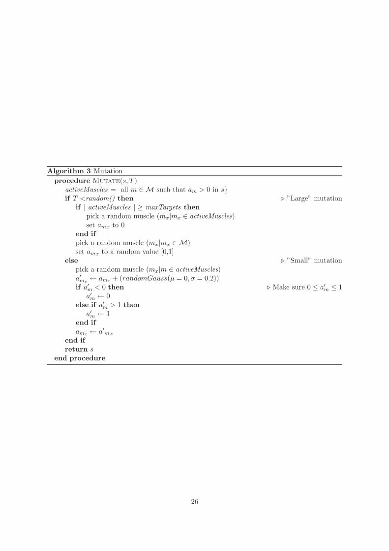
3.1.3 Mutations

After the set of segments S has been initialized, the algorithm will proceed to cycle throughthe segments and create numMutation mutations of this segment. These mutations come intwo types: large and small. A large mutation consists of picking a random muscle parameterfrom M and assigning it a random value between 0 and 1. If there are already maxTargetsactive muscle parameters in the segment, a random active muscle will first be set to 0 (i.e.deactivated). Thus large mutations can result in very different articulations compared to theoriginal segment.

A small mutation, on the other hand, does not add any new muscles to the list of activemuscles, but rather changes the activity of an already active muscle by adding a small valueto its activity am. This value is drawn from a normal distribution with a mean of zero anda standard deviation of 0.2. If the resulting activity value exceeds the upper limit of 1, it isclamped to 1. Likewise, if the resulting value is lower than zero, it will be set to zero, effectivelyremoving this muscle parameter from the list of active targets. The changes wrought by a smallmutation will usually have less impact on the resulting articulation.

A variable T determines the probability of choosing a small mutation rather than a largeone; for each mutation, a random uniform number between 0 and 1 is generated. If this numberis greater than T , a large mutation is made on the segment s; else, a small mutation is made.The value of T increases linearly throughout the simulation, as its value is equal to the numberof the current round divided by the total number of simulation rounds. In this way, the distancebetween the current state and neighbouring states becomes progressively smaller throughoutthe simulation.

Each of the mutated segments is synthesized in Praat, and DTW distances between it andthe other segments in S is calculated, so that the cost f(sij) can be determined for each of themutations {si1 . . . sinumMutations}. The cost of the ‘best’ mutation s′i is then compared to thatof the original segment si; if it is lower, the original segment is replaced by this mutation andthe DTW matrix is updated to reflect the new distances.

3.2 Summary

A pseudocode overview of the main loop (Algorithm 1), the optimization procedure (Algorithm2) and the mutation procedure (Algorithm 3) can be found in this section.

24

Algorithm 1 Initialization. (For this and subsequent algorithms, text in small caps refersto another procedure; if this text is also underlined, it refers to an operation in Praat(Boersma and Weenink 2009).

procedure Main(numRounds,numSegments,numMutations,maxTargets,effortWeight)S ← ∅for i to numSegments do

for j from 1 to maxTargets do ⊲ Initialize segmentspick a random muscle (mx|mx ∈M)amx ← (random([0, 0.3])

end forSynthesize(si)add si to S

end forCalculate DTW distance matrix

S ← Optimize(S,numRounds,numMutations,effortWeight)end procedure

Algorithm 2 Optimization. This is the main loop of the algorithm.

procedure Optimize(S, numRounds,numMutations,effortWeight)we := effortWeightwp := 1−effortWeightfor round from 1 to numRounds do

T ← (round/numRounds)for si ∈ S do

Mutationsi ← ∅for j from 1 to numMutations do

sij ← Mutate (si, T )add sij to MutationsSynthesize(sij )f(sij) = (wd · d(sij ) + we · e(sij ))

end fors ′i ← arg min(f(sij)|sij ∈Mutationsi))if f(s′i) < f(si) then

si ← s′iUpdate DTW matrix

end ifend for

end forreturn S

end procedure

25

Algorithm 3 Mutation

procedure Mutate(s, T )activeMuscles = all m ∈M such that am > 0 in s}if T <random() then ⊲ ”Large” mutation

if | activeMuscles | ≥ maxTargets thenpick a random muscle (mx|mx ∈ activeMuscles)set amx to 0

end ifpick a random muscle (mx|mx ∈M)set amx to a random value [0,1]

else ⊲ ”Small” mutationpick a random muscle (mx|m ∈ activeMuscles)a′mx← amx

+ (randomGauss(µ = 0, σ = 0.2))if a′m < 0 then ⊲ Make sure 0 ≤ a′m ≤ 1

a′m ← 0else if a′m > 1 then

a′m ← 1end ifamx← a′mx

end ifreturn s

end procedure

26

Chapter 4

Evaluation method

In this chapter I will explain how my model of consonant optimization will be tested by com-paring the simulation outcomes to actual spoken language data. In section 4.4, a number ofhypotheses will be stated to test how well the model predicts trends and patterns found innatural consonant inventories.

4.1 Natural language data

The fact that we can speak with some certainty of phonological patterns in the languages of theworld is mainly due to the efforts of numerous descriptive linguists, who have dedicated yearsto the study of previously undescribed languages in remote parts of the world. Data gatheredin this manner have been compiled into various databases, such as the aforementioned UPSID1

(Maddieson and Disner 1984) and P-BASE2 (Mielke 2008). These databases aim to provide arepresentative sample of phonological inventories and processes in the languages of the world.Note that representative must not be interpreted in terms of number of speakers; the fact thatroughly a third of the world’s population speaks some form of Chinese, Spanish, English orArabic (Lewis 2009) must be attributed to historical and political factors, not to properties ofthese languages. Instead, these databases are compiled such that as many language families(groupings of languages known to be related by common descent) as possible are represented.

Information in these phonological databases usually does not come in the form of audiorecordings, but as classifications based on phonetic/phonological features (IPA symbols for P-BASE, an idiosyncratic encoding scheme for UPSID). This means that the notions of perceptualdistinctiveness and articulatory effort (Chapter 2) cannot be applied directly to these data. Tocompare the outcome of the simulations to the crosslinguistic tendencies that can be foundin these datasets, it is therefore necessary to first convert them to the same format, i.e. givesome sort of phonological label to the results. The metric of DTW distance, discussed inChapter 2.2.2, will also be used for converting the articulatory/acoustic data of the simulationsto abstract phonological categories.

4.2 From auditory/articulatory data to phonemic classification

Although the articulatory synthesizer of Boersma was initially chosen for its ability to synthesizemany different types of consonants found in language, the intrinsic and imposed limitations

1http://www.linguistics.ucla.edu/faciliti/sales/software.htm2http://aix1.uottawa.ca/˜jmielke/pbase/index.html

27

Table 4.1: Overview of the 18 consonant labels assigned to the output of the model, sorted by manner(rows) and place (columns) of articulation. The place categories ‘labial’ and ‘labiodental’ have beenmerged; likewise, the coronal consonants and the palatal consonant /j/ have been grouped into a singleplace category. Gaps in the table represent sounds deemed articulatorily impossible, either in naturallanguage or in the articulatory model.

Labial Coronal/palatal Velar Uvular PharyngealPlosive p t k qTrill r ö

Fricative B, v D G K Q(Lateral) approximant w, V ô, l, j î

described in section 2.1 diminish the amount of possible phoneme labelings that may resultfrom the simulations:

• As the source of airflow in the model is determined through fixing the activity of theLungs parameter during search, the results are limited to the class of pulmonic egressivesounds. This excludes implosives from appearing in the simulation.

• As the position of the larynx is fixed in search, ejectives will also not be generated inthe simulations.

• Because timing differences between different articulatory gestures are not allowed underthe constraints I put on Boersma’s model, clicks will not be present in the simulationresults.

• The fixing of the tension of the vocal cords through the Interarytenoid parameter excludesvoicing distinctions.

• The inability of Boersma’s model to accurately synthesize nasals, sibilant fricatives andsibilant affricates effectively excludes these classes from appearing in the simulation.

Based on these limitations, a set of 18 IPA symbols was chosen to label the segments; Table 4.1displays an overview.

The most accurate method of labeling the sounds with these symbols would be to have aphonetically trained linguist annotate them manually. However, annotating the thousands ofsegments generated in the simulations by hand is a very labour-intensive task, and possiblyintroduces the danger of shaping the results toward a desired outcome. I therefore decidedto automate the labeling of segments generated by the model, using the method of dynamictime warping on MFCCs described in section 2.2.2. For this I obtained four sets of comparisontemplate consonants. Each of these sets contains recordings of a male phonetician pronouncingvarious consonant segments in an /a a/ context.3 Figure 4.1 illustrates how the templatesrelated to one another in perceptual space according to the DTW distance metric.

4.2.1 Incorporating articulatory features

As it turned out that labeling the sounds purely on the basis of auditory properties was quiteinaccurate, I have decided to also use articulatory information in classifying the sounds. By

3These sets of recordings were created by Peter Ladefoged, Peter Isotalo, Paul Boersma and JeffMielke. The first two datasets are available online at http://www.ladefogeds.com/vowels/contents.html andhttp://commons.wikimedia.org/wiki/Category:General phonetics respectively. The latter two were obtainedfrom their respective authors.

28

Q

BD

Gîö

K

ô

V

j

k

l

pq

r

t

v

w

-0.25 0.25dimension1

-0.25

0.25

dim

ensi

on2

Figure 4.1: A scatterplot representing the DTW distances between the 18 template segments (averagedover four speakers) used to label the sounds resulting from the simulations. As in Figure 2.7 the 17-dimensional space has been reduced to two dimensions using individual difference scaling.

comparing the shape of the vocal tract in each segment to the shape of a neutral vocal tract, thetube in which the constriction is the smallest may be located. This tube is used to determine theplace of articulation for the sound to be labeled, and limits the set of 18 labels from Table 4.1to the subset with this place feature. If the vocal tract is not notably constricted at any point,the subset will be limited by manner of articulation Approximant instead. Next, dynamictime warping is performed on MFCC representations of the sound and the subset of templatesounds to determine manner of articulation. Algorithm 4 details this procedure.

4.3 Phoneme frequency as a naturalness metric

Now that we have established a method to phonemically label the articulations emerging fromthe simulations, the results can be compared to the crosslinguistic databases mentioned in 4.1.The preferred approach would be to measure closeness of fit of the inventories to those found innatural languages, as for example de Boer (2001) and ten Bosch (1991) did for vowel systems.Unfortunately this is not feasible as the phonemic gaps listed in 4.2 are too large to meaningfullycompare natural consonant systems to the simulation results. Nasal consonants, fricatives andvoicing distinctions are quite common in natural systems, being present in approximately 98%,91% and 68% of languages respectively (Maddieson 2008a), yet cannot be (completely) producedin the current version of the model. The size and variation of natural consonant inventories istherefore not reproducible in the model, making direct comparisons between inventories difficult.

An alternative approach, which is less affected by the phonemic gaps in the current model,is to measure optimality of inventories through the phonemic quality of individual phonemes.As Figure 1.1 shows, the distribution of different phonemes across languages is quite skewed;most phonemes occur only in a fraction of languages, while a handful of phonemes are present inthe inventories of a large majority of languages. This supports the idea that certain individualphonemes are somehow intrinsically preferable to others, perhaps because they occupy a spot

29

Algorithm 4 Algorithm for labeling sounds

procedure LabelSound(s)Calculate VocalTracts from s

for i to 175 do ⊲ (175 = number of tubes in neutral vocal tract)widthsi

= width of tubei in VocalTracts

widthneuti= width of tubei in VocalTractneut

differencei =widthsi

widthneuti

end forsmallestConstrictionIndex = argmin

i∈{1...175}

(differencei)

Calculate standard deviation of differenceif standard deviation< 0.2 then ⊲ No notable constriction

Subset ← Approximant ⊲ Restrict to {/w/,/V/,/ô/,/j/,/l/,î/}else

if smallestConstrictionIndex ≤ 65 thenSubset ← Pharyngeal ⊲ Restrict to {/Q/}

else if smallestConstrictionIndex ≤ 70 thenSubset ← Uvular ⊲ Restrict to {/q/,/ö/,/K/}

else if smallestConstrictionIndex ≤ 80 thenSubset ← Velar ⊲ Restrict to {/k/,/G/,/î/}

else if smallestConstrictionIndex ≤ 160 thenSubset ← Coronal ⊲ Restrict to {/t/,/r/,/D/,/j/,/l/,/ô/}

elseSubset ← Labial ⊲ Restrict to {/V/,/v/,/p/,/B/,/w/}

end ifend ifSynthesize(s)for all 4 speakers in template sets do

for all labels l in Subset doCalculate DTW distance(s, l)

end forNormalize distances

end forCalculate mean distance between speakers per labelreturn label with lowest distance

end procedure

30

Table 4.2: Phoneme labels with their frequencies in P-BASE, and the log10 of this percentage which isused as an index for phoneme optimality.

Label Phoneme group Frequency % in P-BASE Log frequency score

/p/ /p/,/b/ 97.81 1.99

/k/ /k/,/g/ 93.24 1.97

/j/ /j/ 88.50 1.95

/t/ /t/,/d/ 83.75 1.92

/w/ /w/ 78.83 1.90

/l/ /l/ 78.46 1.90

/r/ /r/ 59.67 1.78

/v/ /v/,/f/ 58.39 1.77

/G/ /G/,/x/ 29.19 1.47

/B/ /B/,/F/ 10.76 1.03

/q/ /q/,/ G/ 10.03 1.00

/K/ /K/ 7.48 0.87

/D/ /D/,/T/ 7.29 0.86

/V/ /V/ 5.10 0.71

/Q/ /Q/,/è/ 5.10 0.71

/ô/ /ô/ 3.10 0.49

/î/ /î/ 1.27 0.10

/ö/ /ö/ 1.27 0.10

in the abstract auditory space of Figure 1.4 that is optimal in both auditory terms (distinctivefrom other possible consonants) and in articulatory terms (easy to produce). A good modelof consonant inventories should therefore predict a larger frequency for these phonemes. Forthis reason, I use the estimated frequency of a given phoneme in natural language as a measureof optimality. The source for these frequency estimates is P-BASE (Mielke 2008), as it is themost recent and to my knowledge also largest (in terms of number of represented languages)phoneme database available.

For each of the phoneme labels in table 4.1, I have looked up the relative frequency percent-age of this phoneme over all languages in P-BASE, i.e. the number of languages possessing thisphoneme divided by the total number of languages in the database. In the case of articulationswhich allow voicing distinction in the basic IPA set (i.e. plosives and fricatives), the frequencyof languages containing any phoneme of the voiceless/voiced pair was counted. The base 10logarithm of these percentages was then used as the frequency score for a phoneme (see Table4.3). The naturalness of an inventory is defined as the summed frequency score of all uniquephonemes in the inventory, divided by the size of the simulated inventory numSegments. In-ventories which contain a relatively large number or uncommon or marked phonemes will bescored as less ‘natural’. The next section will discuss a number of phenomena related to markedphonemes that should be explained by a model of consonant inventories, and which can bemeasured using the naturalness metric defined in this section.

31

4.4 Hypotheses

4.4.1 The size principle

A number of trends and common properties found in phoneme systems were briefly mentionedin Chapter 1. One such trend is that the size of a phoneme inventory correlates with thenumber of rare or uncommon phonemes it contains. This is quite visible in vowel inventories,where 3-vowel systems are almost exclusively made up out of the configuration {/a/, /i/, /u/},while larger systems often contain these ‘corner vowels’ plus additional, rarer vowels. Com-puter simulations such as Liljencrants and Lindblom (1972) and de Boer (2001) confirm thatthis trend is replicated in computer simulations operating under simple phonetic principles.Lindblom and Maddieson (1988) show that the size principle also applies to consonant sys-tems; smaller consonant inventories usually contain only members from a ‘basic set’ of about 20consonants. Larger consonant inventories mostly consist of members from this set, plus otherconsonants which are more complex or ‘marked’.

Inventory size can be set as a parameter in the optimization model for consonant inventoriesdescribed in this paper. In a correct model of consonant phoneme distributions, the numberof rare segments in an inventory should correlate positively with the size of the simulatedinventory. The ability of the model to account for the size principle can therefore be tested,using the naturalness metric defined in the previous section and the numSegments parameterdefining the size of the segment inventory S. This will be done in the next chapter.

4.4.2 Balancing maximal distinctiveness and minimal effort

In Chapter 1, the observation that phonemic systems balance between maximal distinctivityand minimal articulatory effort was made. For vowel systems, the first property was shown tobe a deciding factor in the optimization model of Liljencrants and Lindblom (1972). The twoproperties were combined in the vowel optimization model of ten Bosch (1991), showing thatconservation of effort may also play an important role in vowel systems.

Chapter 2 discussed how the two principles are formalized in a cost function for my optimiza-tion model of consonant inventories. If the organization of consonant inventories is organizedalong these lines, it is to be expected that some weighted combination of the effort cost anddistinctivity cost will perform better, i.e. result in an inventory containing more common con-sonants, than just optimizing for optimal distinctivity. This hypothesis can be tested by settingthe relative weight of the effort cost function to various nonzero values and observing the effecton the resulting inventories using the naturalness metric. A comparison of results under varyingsettings of the effortWeight parameter will be made in the next chapter.

32

Chapter 5

Results

In this chapter the simulation results are analyzed. First, an impressionistic analysis of the re-sulting phonemes and inventories is given. Next, the results are quantitatively analysed throughthe method described in 4.2, and the hypotheses put forward in 4.4 will be evaluated.

5.1 Qualitative analysis of results

Praat is able to draw a schematic representation of the vocal tract at any point during anarticulation. By taking several slices per second of an articulation and aligning these with thesynthesized sound resulting from the articulation, I was able to generate movie files from thearticulations. I used these movie files to obtain a general ‘impressionistic-phonetic’ descriptionof the articulatory and acoustic properties of the results.

The resulting inventories generally show perceptual dispersal: several distinct consonantsemerge from the simulations, especially in inventories of sizes 3 and 5. An interesting result isthat the results are almost always articulatorily distinct, even though this was not an optimiza-tion criterion in any of the simulations. Rather, the optimization of perceptual distance seemsto cause, as a side effect, utilization of different muscle groups per segment. Also of interestis that generally, manner of articulation seems to be the optimal way of making perceptualdistinctions within the inventories: the 3-segment inventories often contain a plosive-like sound(usually /t/), a fricative-like sound (often /Q/) and an approximant-like sound. Figure 5.1 showsan example of a 5 segment-inventory found in the model.

/t/ /Q/ /ô/ /p/ /q/

Figure 5.1: Schematic drawing (top) and spectrogram representation (bottom) of a 5-segment inventorythat resulted from search (with EffortWeight=0 ). The phoneme symbols above the images are thoseassigned by the labeling algorithm.

When comparing the types of sounds resulting from the simulation runs to the phonemes ofnatural languages, the most glaringly wrong prediction of the model is that sounds which involve

33

a constriction very far back in the throat are quite abundant in the results. Natural languagescontaining these segments, however, are quite rare (Maddieson 2008b, Mielke 2008). Figure 5.2shows a paurticular type of articulation that showed up quite often in the results, which wasusually labeled as a pharyngeal fricative /Q/. The principally active muscle parameter in thistype of articulation is Mylohyoid, which causes the jaw to move downwards and backwards; asit approaches 1, a constriction is created at the pharynx. If we assume that the rarity of thesetypes of sounds are mainly due to conservation of effort, the conclusion must be that the effortfunction in the current version of the model is not yet sufficient.

Another shortcoming clearly visible in the results is that some of the resulting segmentsare nearly vocalic - that is, the constriction and resulting sound are nearer to a vowel thanto a consonant. This is especially apparent in larger inventories and in simulations wherethe effortWeight parameter was set to a high value. The results were nevertheless labeled asapproximant consonants, rather than vowels.

Figure 5.2: A still of the synthesized vocal tract during a segment that sounds like a pharyngeal fricative/Q/. This type of segment emerged often during the simulations, despite its rarity in natural language.The top of the picture shows a sagittal cross-section of the mouth and throat, the bottom represents therelative tube widths at different points in the vocal tract.

.

Chapter 6.2 discusses how the model might be improved to alleviate the general shortcomingslisted above. The next section will provide a numerical analysis of the optimization results basedon the phoneme labels assigned to the segments.

5.2 Quantitative analysis of results

In the course of a simulation run, the optimization algorithm tries to maximally disperse thesegments in available acoustic space while minimizing the values of the different muscle param-eters. Figure 5.3 shows the effect of this optimization on the DTW distance metric over thecourse of a single simulation run. The results generally show this type of pattern, with the

34

perceptual distance between phonemes quickly rising in the first few rounds of the simulation,after which growth tapers off steadily.

0 1 2 3 4 5 6 7 8 91011121314151617181920210

53.4

106.8

160.2

213.6

267Mean (black), max (blue) and min (red) distances

DT

W d

ista

nce

Round

Figure 5.3: Minimum, mean and maximum DTW distance between segments in one run of the simulation(8 segments, relative effort weight at zero). The pattern shown here is typical for most of the simulationruns.

However, as de Boer (2006) points out, it is not particularly interesting or informative toshow that an optimization algorithm which aims to minimize a cost function reaches a certainminimum. What we are interested in are the linguistic consequences of the optimization process:namely, if dispersion of consonants does indeed take place during the optimization procedure;and if so, under what parameters the end results resemble natural language most closely. Forthis, I will use the naturalness score of phonemes established in 4.3.

5.2.1 Overview

Table 5.2.1 gives an overview of the number of simulations executed to test the model underdifferent values of the effortWeight and numSegments parameters. Effort weight was variouslyset to the values {0, 0.25, 0.5, 0.75, 0.9}. Since setting effort weight to 1 would trivially resultin only ‘effortless’ neutral articulations, this was not attempted in the simulations. For each ofthese settings, inventories of sizes 3, 5 and 8 were created. At least 10 runs of the model wereexecuted under each possible combination of these parameter settings; an additional 10 eachwere executed for effortWeight= 0, to get a more accurate view of the effect of inventory sizeindependent of effort weight.

5.2.2 Results for individual phonemes

Figure 5.4 shows the distribution of segment labels after the final round at the end of all 180simulations. When compared to the frequencies found for these phonemes in P-BASE (see Table4.3, it becomes clear that the predictions of the model are quite inaccurate in some respects.The phonemes /Q/, /V/ and /î/ are much more frequent in the simulation results than theyare in natural language. The latter two, however, are especially frequent in the outcome ofsimulations where the effortWeight parameter has a relatively high value. Figure 5.4 also shows

35

Table 5.1: Overview of the number of simulation runs for the values of the effortWeight and num-Phonemes parameters

number of segments 3 5 8

effortWeight = 0 20 20 20

effortWeight = 0.25 10 10 10

effortWeight = 0.5 10 10 10

effortWeight = 0.75 10 10 10

effortWeight = 0.9 10 10 10

that these two approximant phonemes are much less likely to appear in the results if onlyperceptual distinctivity is taken into account.

The palatal approximant /j/ and the alveolar trill /r/ do not occur at all in the results,while both are attested in a majority of the languages represented in P-BASE. In the case of/r/, it might be that the specific limitations I have imposed on the articulatory model preventthis phoneme from emerging in search; Boersma (1998) reports that the articulatory model isable to synthesize an utterance sounding like /ErE/, but does not specify the settings of thearticulatory parameters required to achieve this.

Two segments which are reported as very frequent in P-base, the bilabial plosive /p/ andthe velar plosive /k/, are a lot rarer in the results. For instance the uvular plosive /q/ is morefrequent in the resulting segments than the velar plosive /k/. In natural language, however, thereverse is the case: /k/ is nearly ubiquitous in the world’s languages, whereas /q/ is present inonly about 10 percent of P-BASE languages. As with the overrepresentation of /Q/, it is likelythe case that the amount of effort involved in making a uvular plosive is not reflected accuratelyin the effort metric.

Figure 5.4: An overview of the frequencies of each of the phoneme labels in the end results for allsimulations (left) and for simulations with effortWeight=0 (right). Some rare phonemes like /Q/, /V/and /î/ occur quite often in the results; some phoneme labels are much less frequent when the relativeweight of effort cost is low.

36

Table 5.2: p values of 2-sided t-tests comparing the effect of zero effort to the effort values 0.25, 0.5, 0.75and 0.9. Degrees of freedom was 28 for all tests. Starred values are significant at α < 0.05

we=0.25 we=0.5 we=0.75 we=0.9

3 phonemes 0.39392 0.83581 0.49550 0.00002*

5 phonemes 0.56597 0.15946 0.17014 0.00001*

8 phonemes 0.94417 0.50545 0.15307 0.00000*

5.2.3 Effect of effort cost weight on naturalness

To test the effects of varying the effort parameter, the results for several simulation runs underdiffering values of the effortWeight parameter were compared to simulation runs with thisparameter set to zero. Significance was tested using Student’s t-test (two-sided, α = 0.05).Figure 5.5 and Table 5.2 summarize the results.

0

0.4

0.8

1.2

1.6

2

0 0.25 0.5 0.75 0.9Effort weight

Freq

uenc

y sc

ore

Number of segments: 3

0

0.4

0.8

1.2

1.6

2

0 0.25 0.5 0.75 0.9Effort weight

Freq

uenc

y sc

ore

Number of segments: 5

0

0.4

0.8

1.2

1.6

2

0 0.25 0.5 0.75 0.9Effort weight

Freq

uenc

y sc

ore

Number of segments: 8

Figure 5.5: Comparing the effect of different values for the effortWeight parameter. The vertical axisshows the naturalness score (summed frequency score of all unique phoneme labels divided by numSeg-ments). Red bars show plus and minus one standard deviation. Regardless of the number of segments,in the range from 0.25 to 0.75 no significant effect of effort is found; if effortWeight is 0.9, there is asignificant negative effect on the naturalness of the resulting inventory.

The results show that for intermediate values (0,25, 0.5, 0.75) of the effortWeight parameter,no significant effect on the naturalness of the resulting inventories is found. If effortWeight is setto the high value of 0.9, there is a significant negative impact on naturalness of the results. Thisis caused by the large number of (relatively rare) approximant phonemes appearing in inventoriesgenerated under a high value for the effort weight parameter, as shown in the previous section.

5.2.4 Effect of inventory size on naturalness

Figure 5.6 shows the naturalness scores for inventories of 3, 5 and 8 segments under variousvalues of the effortWeight parameter. To test the hypothesis that rarer phonemes should appearmore often in larger inventories (as is generally the case in natural language), I calculated thePearson’s ρ correlation coefficient between the value of the parameter numSegments and thenaturalness score of the inventories generated with effortWeight = 0. The correlation is -0.214,which is not significant (α = 0.025, one-tailed, df=58). This indicates that the model does notaccurately predict the size principle (Lindblom and Maddieson 1988) acting on the consonantinventories of natural languages.

37

0

0.4

0.8

1.2

1.6

2

3 5 8Number of segments

Effort weight: 0

0

0.4

0.8

1.2

1.6

2

3 5 8Number of segments

Freq

uenc

y sc

ore

Effort weight: 0

0

0.4

0.8

1.2

1.6

2

3 5 8Number of segments

Effort weight: 0.25

0

0.4

0.8

1.2

1.6

2

3 5 8Number of segments

Effort weight: 0.5

0

0.4

0.8

1.2

1.6

2

3 5 8Number of segments

Freq

uenc

y sc

ore

Effort weight: 0.75

0

0.4

0.8

1.2

1.6

2

3 5 8Number of segments

Effort weight: 0.9

0

0.4

0.8

1.2

1.6

2

3 5 8Number of segments

All effort weight values

Figure 5.6: Effect of inventory size on naturalness. As in figure 5.5, the naturalness scores indicated onthe vertical axis, and red bars indicate plus and minus one standard deviation.

38

Chapter 6

Conclusion and discussion

6.1 Summary and analysis of results

This paper presents a computational model of consonant inventories in natural language. Themodel is based on previous simulations of vowel systems, in which vowel configurations similarto those of natural languages were found by optimizing for maximal perceptual contrast andminimal articulatory effort. These results support an emergentist explanation of crosslinguis-tic patterns in phoneme inventories. Consonant inventories, although more diverse than vowelinventories, are often assumed to emerge under similar constraints. To extend the vowel opti-mization methods to the more complex domain of consonants, a novel optimization method wasdeveloped. This method uses an articulatory synthesizer (Boersma 1998) to explore the articu-latory and acoustic space available in consonant production, and a model of acoustic dispersionbased on Dynamic Time Warping (DTW) of pairs of signals thus synthesized. DTW was alsoused to give a phonemic label to the resulting sound signals.

The articulatory model used to produce consonants was regrettably found to be incapableof synthesizing a number of consonant sounds that are quite abundant in natural language.As a consequence, the phonemic repertoire available to the optimisation model is limited incomparison to that of real speakers. Because of this, direct comparison of the configurationsemerging from the model to those found in the various languages and language families of theworld was not feasible. Instead, an alternative evaluation method was developed, in which thenaturalness of an inventory was defined as a function of the relative frequencies of its membersin a database of phonological inventories (P-BASE, Mielke 2008).

A qualitative analysis of the resulting inventories confirmed that dispersion of consonantstakes place in the optimization algorithm. As in natural language, certain phonemes werepresent in the inventories much more frequently than others; at the same time no single ‘op-timal’ solution emerged from the results. This is probably due to the complex shape of theoptimization landscape, and in fact reflects the diversity of consonant systems found in language(there is generally much greater variety for consonants than there is for vowels). However, theresults are not very accurate with respect to the quality of the resulting consonants. Consonantphonemes which are abundant in natural languages, such as /k/, /j/ and /p/, were absent oronly marginally present in the simulation results. At the same time, several phonemes whichoccur only rarely in natural language such as /Q/ and /q/ are quite frequent in the labeledresults. Generally, the model seems too inclined towards consonants made in the back of theoropharyngeal cavity. The optimality of these consonants according to the model is not reflectedin natural language data.

The naturalness metric was used to test two hypotheses. The first concerns the size principle,which states that there is a positive correlation between the number of phonemes in an inventory

39

and the relative number of rare or more complex phonemes it contains. This would translate toa lower naturalness for larger inventories in the model. However, no significant correlation wasfound between the number of phonemes modeled and the naturalness scores of the resultinginventories. The second hypothesis concerned the proposed balance between maximal inter-phoneme distinctiveness and minimal articulatory effort. Simulation results did not confirmthat these constraints apply to consonant inventories: varying the relative weight of articulatoryeffort in the cost function did not have a significant positive effect on naturalness.

Quantitative analysis of the results thus supports the conclusion that unlike vowel inven-tories, patterns in consonant inventories do not emerge from a combination of the phoneticprinciples of minimal effort and maximal distinctiveness. However, I believe the qualitativeanalysis suggests that the optimization approach may not be a dead end. The overrepresenta-tion of crosslinguistically rare segments in the results indicates that some aspects of consonantinventory optimality are not represented faithfully in the current version of the model. The nextsection therefore lists a number of improvements that could be made on the model to betteraccount for linguistic data.

6.2 Future work

6.2.1 Improving the optimization model

As set out in chapter 2.1, the articulatory model of Boersma (1998) used in the optimizationmodel described in this paper was constrained in a number of ways. Some of these constraintsare intrinsic to the synthesizer, such as the inability to accurately synthesize sibilants andnasals. I imposed additional constraints to limit the size of the search space. Abstracting fromcertain properties of sounds is to some extent necessary in a phonetic model, but in this casethe predictive power of the model is too severely hampered by the abstractions. Given itsinability to synthesize the important classes of nasal and sibilant consonants, in retrospect thearticulatory model of Boersma does not suffice for accurate modelling of consonant inventories.In order to improve the optimization model it will therefore be necessary to either switch toanother articulatory model, such as that of Birkholz (2005), or to extend Boersma’s model sothat it can account for a richer set of sounds. Increasing the phonetic space available to themodel will also allow for a better comparison of model output to natural language data.

While increasing weight of the effort cost parameter was shown to impact the results, itdid not have the hypothesized effect of increasing naturalness of the resulting inventories. Ibelieve this does not disprove the notion of conservation of effort ; rather, the effort cost functionintroduced in this paper likely does not reflect actual articulatory effort well enough. A first steptowards improving the effort cost function is probably to increase the differences in effort cost forindividual muscle parameters; particularly the articulations resulting in uvular and pharyngealconstrictions should be punished more severely in the effort cost function. The assumption thateffort is directly determined by muscle activity may also be too naive. Considerations like theprecision required for a gesture (or robustness to articulatory fluctuations, see Stevens 1972)may also contribute to the concept of articulatory effort.

Perceptual distance is defined purely in auditory terms in the current model. However, whilenot strictly necessary to acquire and use speech, visual perception also plays an important role inspeech perception, aiding in discriminating speech distorted by noise (Sumby and Pollack 1954)and able to overrule auditory information under certain circumstances (McGurk and MacDonald1976). It is plausible that visually distinct articulations, like bilabials, may be generally pre-ferred in the world’s languages for these reasons. The lack of a visual modality in the currentmodel may be partially responsible for the unrealistic proclivity toward sounds made in the

40

back of the throat.In terms of evaluation of the results, the automatic labeling of simulated phonemes through

DTW comparison with template phonemes is another component of the model that can be im-proved. While manually labeling large numbers of synthesized phonemes is too labour-intensiveto classify all results by hand, the classification algorithm could be improved through supervisedtraining on a number of hand-labeled examples. For a more principled analysis of the results, itis also necessary to develop an evaluation method which is able to compare resulting inventoriesas a whole to the inventories of natural languages, instead of basing naturalness of inventorieson properties of its individual members. A feature-based approach similar to that of Mielke(2005) might be taken here.

Finally, the current model could be improved by modelling sound variation in a largercontext. As is, the model only allows for limited variation within a static /@ @/ context. Thisserves to keep the search space of the model, and the range of possible results, within reasonablelimits. Actual articulation of speech sounds, however, is often conditioned by the phonemicenvironment in which the sound occurs. A more thorough model of consonant inventoriesshould therefore be able to account for this, for instance by allowing more variation on thevowel context surrounding the synthesized consonants.

6.2.2 Towards a non-teleological, speaker-oriented model

The model described in this paper optimizes at the level of the language. While many commonsound changes and inventory states can be stated in terms of global processes such as acousticdispersion and effort minimization, this ultimately does not explain the mechanisms responsiblefor sound change and inventory formation. Rather, these global processes are thought to beset in motion by local processes at the level of the speaker and hearer (Ohala 1981, Blevins2004). Computer simulations confirm that optimal phoneme inventories may emerge as a resultof small-scale interactions between simulated individuals (agents) who do not explicitly aim tooptimize the inventory (de Boer 2001).

Many of the components of the current model, such as the use of articulatory synthesisand the use of techniques from speech recognition to define perceptual similarity or distance,could probably be incorporated without much trouble in an agent-based model of consonantinventories. An agent-based model could also incorporate the concept of learnability, reflectingthe fact that some articulations are more difficult to master than others, and that learned motorgestures can be reused in other articulations. However, as the computational cost of realisticarticulatory synthesis is quite high at the moment of writing, the computing power required formodelling even a modest number of interacting agents equipped with such a synthesizer mayyet be too substantial.

41

Chapter 7

Acknowledgements

I am grateful to my supervisors David Weenink and Maarten van Someren for their guidance,suggestions and discussions during the time spent on this report. I also thank Remko Schafor agreeing to partake in the examination committee. Thanks also go out to Paul Boersmafor answering my questions on the articulatory synthesizer and on one occasion fixing a veryspecific feature that I needed in Praat. For commenting on some ideas and earlier drafts of thereport I thank Adi Ben-Arieh, Titia Benders and Tessa Verhoef. For allowing me to use theirrecordings of various IPA consonants I thank Paul Boersma and Jeff Mielke.

Finally, I thank all my loved ones for their patience and trust, even at times when I had lostthese myself, during the long months spent on this thesis.

42

Bibliography

(1999). Handbook of the International Phonetic Association : A Guide to the Use of the Inter-national Phonetic Alphabet. International Phonetic Association.

Allen, W. (1989). Vox Latina: a guide to the pronunciation of classical Latin. CambridgeUniversity Press.

Battye, A., Hintze, M., and Rowlett, P. (2000). The French language today: a linguistic intro-duction. Routledge, London.

Birkholz, P. (2005). 3D-artikulatorische Sprachsynthese. Logos, Berlin.

Bladon, A. (1983). Two-formant models of vowel perception: shortcomings and enhancements.Speech Communication, 2(4):305–313.

Blevins, J. (2004). Evolutionary phonology: The emergence of sound patterns. CambridgeUniversity Press.

Boe, L., Heim, J., Honda, K., and Maeda, S. (2002). The potential Neandertal vowel space wasas large as that of modern humans. Journal of Phonetics, 30(3):465–484.

Boersma, P. (1989). Modelling the distribution of consonant inventories by taking a function-alist approach to sound change. In Proceedings of the Institute of Phonetic Sciences of theUniversity of Amsterdam, volume 13, pages 107–123.

Boersma, P. (1998). Functional phonology. Holland Academic Graphics, Den Haag.

Boersma, P. and Hamann, S. (2008). The evolution of auditory dispersion in bidirectionalconstraint grammars. Phonology, 25(02):217–270.

Boersma, P. and Weenink, D. (2009). Praat: doing phonetics by computer (v 5.1.03). Computerprogram.

Bridle, J. and Brown, M. (1974). An experimental automatic word recognition system. Technicalreport, Joint Speech Research Unit, Ruislip, England.

Caramazza, A., Chialant, D., Capasso, R., and Miceli, G. (2000). Separable processing ofconsonants and vowels. Nature, 403(6768):428–430.

Chomsky, N. (1965). Aspects of the Theory of Syntax. MIT press.

Chomsky, N. and Halle, M. (1968). The sound pattern of English. Studies in Language. Harper& Row, New York.

Clark, J., Yallop, C., and Fletcher, J. (2006). An introduction to phonetics and phonology.Wiley-Blackwell.

43

Davis, S. and Mermelstein, P. (1980). Comparison of parametric representations for monosyl-labic word recognition in continuously spoken sentences. IEEE Transactions on Acoustics,Speech and Signal Processing, 28(4):357–366.

de Boer, B. (2001). The origins of vowel systems. Oxford University Press.

de Boer, B. (2006). Computer modelling as a tool for understanding language evolution. In Gon-tier, N., Van Bendegem, J. P., and Aerts, D., editors, Evolutionary Epistemology, Languageand Culture, pages 381–406. Springer.

de Boer, B. (2008). The acoustic role of supralaryngeal air sacs. Journal of the AcousticalSociety of America, 123(5):3779–3779.

Delattre, P., Liberman, A., and Cooper, F. (1955). Acoustic loci and transitional cues forconsonants. The Journal of the Acoustical Society of America, 27:769.

Eulitz, C. and Lahiri, A. (2004). Neurobiological evidence for abstract phonological represen-tations in the mental lexicon during speech recognition. Journal of cognitive neuroscience,16(4):577–583.

Fant, G. (1970). Acoustic theory of speech production. Mouton De Gruyter, den Haag.

Harris, K. (1958). Cues for the discrimination of American English fricatives in spoken syllables.Language and Speech, 1(1):1–7.

Jurafsky, D. and Martin, J. (2008). Speech and language processing. Prentice Hall.

Kazanina, N., Phillips, C., and Idsardi, W. (2006). The influence of meaning on the perceptionof speech sounds. Proceedings of the National Academy of Sciences, 103(30):11381.

Kelly, J. L. and Lochbaum, C. C. (1962). Speech synthesis. In Proceedings of the FourthInternational Congress on Acoustics, pages 1–4, Copenhagen, Denmark.

Kirby, S. (2001). Spontaneous evolution of linguistic structure-an iterated learning model of theemergence of regularity and irregularity. IEEE Transactions on Evolutionary Computation,5(2):102–110.

Kirby, S. and Hurford, J. (2002). The emergence of linguistic structure: An overview of theiterated learning model. In Cangelosi, A. and Parisi, D., editors, Simulating the Evolution ofLanguage, chapter 6, pages 121–148. Springer Verlag, London.

Klatt, D. (1987). Review of text-to-speech conversion for English. Journal of the AcousticalSociety of America, 82(3):737–793.

Klein, W., Plomp, R., and Pols, L. (1970). Vowel Spectra, Vowel Spaces, and Vowel Identifica-tion. The Journal of the Acoustical Society of America, 48:999.

Kuhl, P. (1981). Discrimination of speech by nonhuman animals: Basic auditory sensitivitiesconducive to the perception of speech-sound categories. The Journal of the Acoustical Societyof America, 70:340.

Ladefoged, P. (2005). Vowels and consonants: An introduction to the sounds of languages.Blackwell, London.

Lasarcyk, E. (2007). Investigating larynx height with an articulatory speech synthesizer. InProceedings of the 16 th ICPhS, Saarbrucken.

44

Lewis, M. P., editor (2009). Ethnologue: Languages of the World, Sixteenth edition. SILInternational, Dallas, Texas. Online version: http://www.ethnologue.com/.

Liljencrants, J. and Lindblom, B. (1972). Numerical simulation of vowel quality systems: Therole of perceptual contrast. Language, 48:839–862.

Lindblom, B. and Maddieson, I. (1988). Phonetic universals in consonant systems. In Language,speech and mind. Studies in honour of Victoria A. Fromkin, chapter 6, pages 62–78.

Lisker, L. and Abramson, A. S. (1963). Crosslanguage study of voicing in initial stops. TheJournal of the Acoustical Society of America, 35(11):1889–1890.

Maddieson, I. (2008a). Absence of common consonants. In Haspelmath, M., Dryer, M. S., Gil,D., and Comrie, B., editors, World Atlas of Language Structures Online. Max Planck DigitalLibrary, Munich. Available online at http://wals.info/feature/8. Accessed on August 4 2009.

Maddieson, I. (2008b). Presence of uncommon consonants. In Haspelmath, M., Dryer, M. S.,Gil, D., and Comrie, B., editors, World Atlas of Language Structures Online. Max PlanckDigital Library, Munich. Available online at http://wals.info/feature/19. Accessed on August4 2009.

Maddieson, I. and Disner, S. (1984). Patterns of sounds. Cambridge university press New York.

Maeda, S. (1982). A digital simulation method of the vocal tract system. Speech Communication,1(3-4):199–229.

McGurk, H. and MacDonald, J. (1976). Hearing lips and seeing voices. Nature, 264(5588):746–748.

Mermelstein, P. (1973). Articulatory model for the study of speech production. The Journal ofthe Acoustical Society of America, 53:1070.

Mielke, J. (2005). Modeling distinctive feature emergence. In Proceedings of the West CoastConference on Formal Linguistics, volume 24, pages 281–289.

Mielke, J. (2008). The emergence of distinctive features. Oxford Univ Press.

Moreton, E. (2008). Analytic bias and phonological typology. Phonology, 25(01):83–127.

Ohala, J. (1981). The listener as a source of sound change. parasession on language and behavior,pages 178–203.

Oudeyer, P. (2001). The origins of syllable systems: an operational model. In proceedings ofthe International Conference on Cognitive science, COGSCI.

Pols, L., Tromp, H., and Plomp, R. (1973). Frequency analysis of Dutch vowels from 50 malespeakers. The journal of the Acoustical Society of America, 53:1093.

Prince, A. and Smolensky, P. (1993). Optimality theory: Constraint interaction in generativegrammar. Manuscript, Rutgers University and University of Colorado at Boulder. Availableat ROA.

Roach, P. (2000). English phonetics and phonology: A practical course. Cambridge UniversityPress, 3 edition.

45

Sakoe, H. and Chiba, S. (1978). Dynamic programming algorithm optimization for spoken wordrecognition. IEEE Transactions on acoustics, speech and signal processing, 26(1):43–49.

Schwartz, J., Boe, L., Vallee, N., and Abry, C. (1997). The dispersion-focalization theory ofvowel systems. Journal of phonetics, 25(3):255–286.

Shadle, C. and Damper, R. (2001). Prospects for articulatory synthesis: A position paper. In4th ISCA Tutorial and Research Workshop (ITRW) on Speech Synthesis. ISCA.

Sroka, J. J. and Braida, L. D. (2005). Human and machine consonant recognition. SpeechCommunication, 45(4):401–423.

Stevens, K. (1972). The quantal nature of speech: Evidence from articulatory-acoustic data,pages 51–66. McGraw-Hill Companies.

Stevens, S. S. and Volkmann, J. (1940). The relation of pitch to frequency: A revised scale.The American Journal of Psychology, 53(3):329–353.

Sumby, W. H. and Pollack, I. (1954). Visual contribution to speech intelligibility in noise. TheJournal of the Acoustical Society of America, 26(2):212–215.

ten Bosch, L. (1991). On the Structure of Vowel Systems. Aspects of an extended vowel modelusing effort and contrast. PhD thesis, Universiteit van Amsterdam.

Traill, A. (1985). Phonetic and phonological studies of !Xoo Bushman. John Benjamins PubCo.

Traunmuller, H. (1981). Perceptual dimension of openness in vowels. The Journal of theAcoustical Society of America, 69:1465.

Trubetzkoy, N. (1939). Grundzuge der Phonologie [Principles of Phonology, translated 1969 byC. Baltaxe]. Berkeley and Los Angeles: University of California Press.

Tzanetakis, G. and Cook, P. (2002). Musical genre classification of audio signals. IEEE Trans-actions on speech and audio processing, 10(5):293–302.

van Leussen, J.-W. (2008). Emergent optimal vowel systems. Master’s thesis, University ofAmsterdam. Available as ROA-1006 at http://roa.rutgers.edu.

Viterbi, A. (1967). Error bounds for convolutional codes and an asymptotically optimum de-coding algorithm. IEEE transactions on Information Theory, 13(2):260–269.

Zipf, G. (1949). Human behavior and the principle of least effort: An introduction to humanecology. Addison-Wesley Press, Massachusetts.

Zuidema, W. and de Boer, B. (2009). The evolution of combinatorial phonology. Journal ofPhonetics, 37(2):125–144.

46