A Deep Belief Network for the Acoustic-Articulatory ... · A Deep Belief Network for the Acoustic-Articulatory Inversion Mapping ... The acoustic-articulatory inversion mapping problem

A Deep Belief Network for the Acoustic-Articulatory

Inversion Mapping Problem

Benigno Uría

TH

E

U N I V E RS

IT

Y

OF

ED I N B U

RG

H

Master of Science

Artificial Intelligence

School of Informatics

University of Edinburgh

2011

Abstract

In this work, we implement a deep belief network for the acoustic-articulatory inversion

mapping problem.

We find that adding up to 3 hidden-layers improves inversion accuracy. We also show this

is due to the higher expressive capability of a deep model and not a consequence of adding

more adjustable parameters. Besides, we show unsupervised pretraining of the system im-

proves its performance in all cases, even for a 1 hidden-layer model.

Our implementation obtained an average root mean square error of 0.95 mm on the MNGU0

test dataset, beating all previously published results.

iii

Acknowledgements

Thanks to Steve Renals and Korin Richmond, for their encouragement, patience and teach-

ings. It has been a pleasure working with such knowledgeable and approachable supervi-

sors.

Thanks as well to Iain Murray, and all the people at the ANC, for giving me unlimited

access to their GPU equipment. Without them I would still be waiting.

iv

Declaration

I declare that this thesis was composed by myself, that the work contained herein is my

own except where explicitly stated otherwise in the text, and that this work has not been

submitted for any other degree or professional qualification except as specified.

(Benigno Uría)

v

Contents

1 Introduction 1

2 Background 5

2.1 Previous approaches to articulatory inversion . . . . . . . . . . . . . . . . 5

2.1.1 Early approaches: synthetic datasets . . . . . . . . . . . . . . . . . 5

2.1.2 Articulography and EMA datasets . . . . . . . . . . . . . . . . . . 6

2.1.3 Modern approaches: Learning from EMA data . . . . . . . . . . . 8

2.2 Deep architectures . . . . . . . . . . . . . . . . . . . . . . . . . . . . . . 10

2.2.1 Introduction . . . . . . . . . . . . . . . . . . . . . . . . . . . . . . 10

2.2.2 Restricted Boltzmann machines . . . . . . . . . . . . . . . . . . . 11

2.2.3 Deep belief networks . . . . . . . . . . . . . . . . . . . . . . . . . 14

2.3 Deep belief networks in phone recognition . . . . . . . . . . . . . . . . . . 16

3 Data and Evaluation Criteria 21

3.1 The MNGU0 dataset . . . . . . . . . . . . . . . . . . . . . . . . . . . . . 21

3.1.1 Data setup . . . . . . . . . . . . . . . . . . . . . . . . . . . . . . . 22

3.2 Evaluation criteria . . . . . . . . . . . . . . . . . . . . . . . . . . . . . . . 23

3.3 Benchmarks . . . . . . . . . . . . . . . . . . . . . . . . . . . . . . . . . . 23

4 Implementation and Results 25

4.1 A deep belief network for articulatory inversion . . . . . . . . . . . . . . . 25

4.1.1 Pretraining . . . . . . . . . . . . . . . . . . . . . . . . . . . . . . 25

4.1.2 Adaptation of the DBN for articulatory regression . . . . . . . . . . 29

4.1.3 Results . . . . . . . . . . . . . . . . . . . . . . . . . . . . . . . . 30

4.2 Low-pass filtering . . . . . . . . . . . . . . . . . . . . . . . . . . . . . . . 35

4.3 Output augmentation, multitask learning . . . . . . . . . . . . . . . . . . . 39

5 Conclusion 45

5.1 Contributions . . . . . . . . . . . . . . . . . . . . . . . . . . . . . . . . . 45

5.2 Limitations . . . . . . . . . . . . . . . . . . . . . . . . . . . . . . . . . . 45

5.3 Future work . . . . . . . . . . . . . . . . . . . . . . . . . . . . . . . . . . 46

vii

Bibliography 47

A Computational setup 53

viii

Chapter 1

Introduction

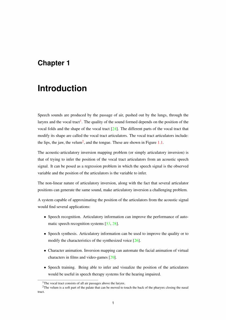
Speech sounds are produced by the passage of air, pushed out by the lungs, through the

larynx and the vocal tract1. The quality of the sound formed depends on the position of the

vocal folds and the shape of the vocal tract [24]. The different parts of the vocal tract that

modify its shape are called the vocal tract articulators. The vocal tract articulators include:

the lips, the jaw, the velum2, and the tongue. These are shown in Figure 1.1.

The acoustic-articulatory inversion mapping problem (or simply articulatory inversion) is

that of trying to infer the position of the vocal tract articulators from an acoustic speech

signal. It can be posed as a regression problem in which the speech signal is the observed

variable and the position of the articulators is the variable to infer.

The non-linear nature of articulatory inversion, along with the fact that several articulator

positions can generate the same sound, make articulatory inversion a challenging problem.

A system capable of approximating the position of the articulators from the acoustic signal

would find several applications:

• Speech recognition. Articulatory information can improve the performance of auto-

matic speech recognition systems [53, 28].

• Speech synthesis. Articulatory information can be used to improve the quality or to

modify the characteristics of the synthesized voice [26].

• Character animation. Inversion mapping can automate the facial animation of virtual

characters in films and video-games [20].

• Speech training. Being able to infer and visualize the position of the articulators

would be useful in speech therapy systems for the hearing impaired.

1The vocal tract consists of all air passages above the larynx.2The velum is a soft part of the palate that can be moved to touch the back of the pharynx closing the nasal

tract.

1

2 Chapter 1. Introduction

Upper lip

Lower lip

JawTongue

Velum

Figure 1.1: Vocal tract articulators shown on a midsagittal section of the head.

• Very low bit-rate speech coding. Speech can be synthesized back from the position

of the vocal tract articulators, and very low sampling rates are needed.

Several mathematical techniques have been applied in the past to tackle the articulatory

inversion problem. The introduction of rich articulography datasets of precise quantitative

articulatory position data along with recordings of the acoustic data produced, has made it

possible to use standard machine learning methodologies like artificial neural networks [44]

or hidden Markov models [19, 56].

Artificial neural networks with more than one or two hidden layers have usually been con-

sidered too difficult to train to be of practical use [3]. However, they have become a practical

option after new theoretical insights on the potential advantages of this kind of deep archi-

tectures [3], and the introduction in 2006 of an algorithm capable of training an artificial

neural network with many hidden layers, by first training a deep generative model called

deep belief network [18].

Deep architectures (more specifically, deep belief networks) have recently been used to

obtain state-of-the-art accuracies in phone classification [30, 10, 33, 32, 31, 22] (i.e. in

classifying speech acoustic signals into phonemes). Motivated by these successes in phone

recognition, and given its similarities with articulatory inversion, we hypothesised a deep

belief network would be able to obtain high accuracy in articulatory inversion.

In this work we have implemented a deep belief network for articulatory inversion. We

have evaluated its performance using the MNGU0 test dataset for which we obtained a

root mean squared error (RMSE) of 0.95 mm. A significant improvement with respect

3

to the best previously published results of 0.99 mm obtained by Richmond [46] using a

trajectory mixture density network. This favourable result leads us to conclude that deep

architectures are a suitable approach to articulatory inversion. Furthermore, given that our

implementation uses a very simple dynamical model, we hypothesise an even higher degree

of accuracy could be obtained using a more elaborate trajectory model which we propose

as future work.

The rest of this dissertation is organized as follows: in Chapter 2, we will review the pre-

vious literature on articulatory inversion. After that we will introduce the functioning of

deep architectures, focusing on deep belief networks. Then, we will review the previous

literature on the use of deep belief networks in speech processingm more specifically, in

phone classification. In Chapter 3, we will introduce the dataset and evaluation criteria we

will use to judge the performance of our system. In Chapter 4, we will detail our implemen-

tation, analyse its performance and discuss the different implementation variants we have

tried, comparing them with each other and with results from previous research. To finish, in

Chapter 5 we will draw some conclusions and outline future research directions we intend

to pursue.

Chapter 2

Background

2.1 Previous approaches to articulatory inversion

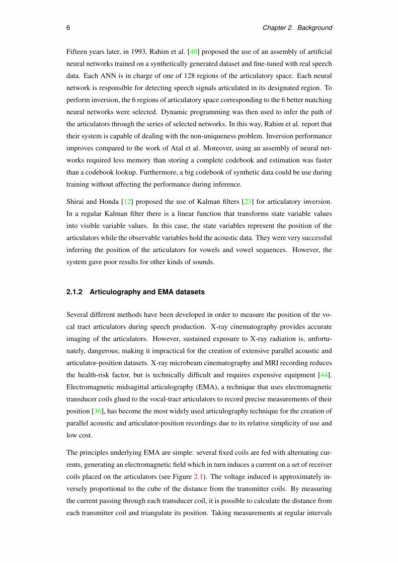
2.1.1 Early approaches: synthetic datasets

Early work on the acoustic-articulatory inversion problem was hampered by the lack, at the

time, of precise quantitative data on articulator-position acoustic-signal correspondences.

Two different approaches were taken to avoid this obstacle:

1. Inversion by mathematical analysis of the speech signal in order to calculate the size

of the resonance tubes that could have produced it. These techniques have several

disadvantages: they are only suitable for a small subset of sounds like vowels and

some voiced consonants, it is not easy to find out whether the areas calculated are

physically possible to articulate, and they require special measurement techniques of

the acoustic signal [44].

2. Use of computer simulations of the vocal tract in order to produce synthetic datasets

of articulator-position to acoustic-output correspondences [1, 40, 12], which are then

used to train standard regression techniques.

The work of Atal et al. [1] in 1978 is an example of inversion using synthetic datasets. In

their work, the authors generated a codebook of many articulator-position acoustic-output

pairs by simulating a vocal tract while regularly varying four articulator position parame-

ters. Once the codebook had been created, inversion was done simply by looking up in the

codebook the articulator configuration corresponding to the best match for the acoustic in-

put to invert. In their work, Atal et al. noticed that some sounds can be produced by several

articulator configurations. The solution, therefore, may be non-unique, making articulatory

inversion an ill-poised problem.

5

6 Chapter 2. Background

Fifteen years later, in 1993, Rahim et al. [40] proposed the use of an assembly of artificial

neural networks trained on a synthetically generated dataset and fine-tuned with real speech

data. Each ANN is in charge of one of 128 regions of the articulatory space. Each neural

network is responsible for detecting speech signals articulated in its designated region. To

perform inversion, the 6 regions of articulatory space corresponding to the 6 better matching

neural networks were selected. Dynamic programming was then used to infer the path of

the articulators through the series of selected networks. In this way, Rahim et al. report that

their system is capable of dealing with the non-uniqueness problem. Inversion performance

improves compared to the work of Atal et al. Moreover, using an assembly of neural net-

works required less memory than storing a complete codebook and estimation was faster

than a codebook lookup. Furthermore, a big codebook of synthetic data could be use during

training without affecting the performance during inference.

Shirai and Honda [12] proposed the use of Kalman filters [23] for articulatory inversion.

In a regular Kalman filter there is a linear function that transforms state variable values

into visible variable values. In this case, the state variables represent the position of the

articulators while the observable variables hold the acoustic data. They were very successful

inferring the position of the articulators for vowels and vowel sequences. However, the

system gave poor results for other kinds of sounds.

2.1.2 Articulography and EMA datasets

Several different methods have been developed in order to measure the position of the vo-

cal tract articulators during speech production. X-ray cinematography provides accurate

imaging of the articulators. However, sustained exposure to X-ray radiation is, unfortu-

nately, dangerous; making it impractical for the creation of extensive parallel acoustic and

articulator-position datasets. X-ray microbeam cinematography and MRI recording reduces

the health-risk factor, but is technically difficult and requires expensive equipment [44].

Electromagnetic midsagittal articulography (EMA), a technique that uses electromagnetic

transducer coils glued to the vocal-tract articulators to record precise measurements of their

position [36], has become the most widely used articulography technique for the creation of

parallel acoustic and articulator-position recordings due to its relative simplicity of use and

low cost.

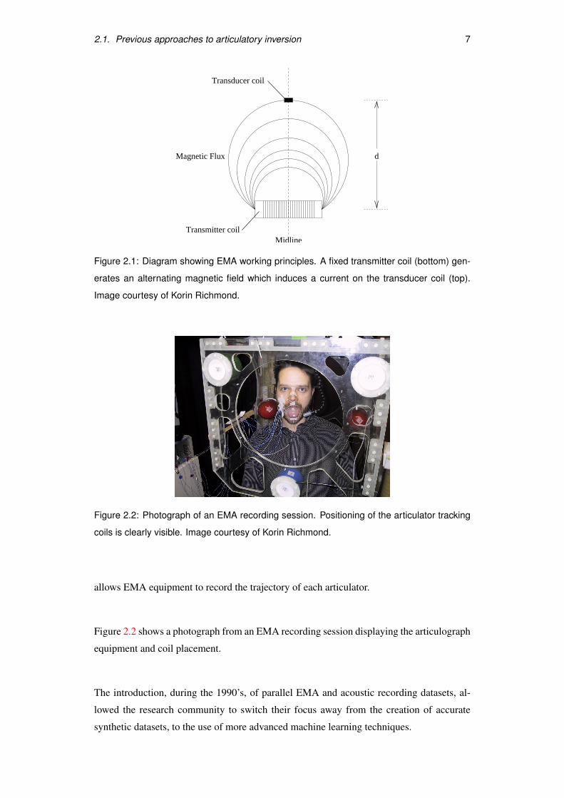
The principles underlying EMA are simple: several fixed coils are fed with alternating cur-

rents, generating an electromagnetic field which in turn induces a current on a set of receiver

coils placed on the articulators (see Figure 2.1). The voltage induced is approximately in-

versely proportional to the cube of the distance from the transmitter coils. By measuring

the current passing through each transducer coil, it is possible to calculate the distance from

each transmitter coil and triangulate its position. Taking measurements at regular intervals

2.1. Previous approaches to articulatory inversion 7

Midline

dMagnetic Flux

Transducer coil

Transmitter coil

Figure 2.1: Diagram showing EMA working principles. A fixed transmitter coil (bottom) gen-

erates an alternating magnetic field which induces a current on the transducer coil (top).

Image courtesy of Korin Richmond.

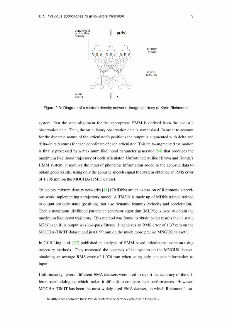
Figure 2.2: Photograph of an EMA recording session. Positioning of the articulator tracking

coils is clearly visible. Image courtesy of Korin Richmond.

allows EMA equipment to record the trajectory of each articulator.

Figure 2.2 shows a photograph from an EMA recording session displaying the articulograph

equipment and coil placement.

The introduction, during the 1990’s, of parallel EMA and acoustic recording datasets, al-

lowed the research community to switch their focus away from the creation of accurate

synthetic datasets, to the use of more advanced machine learning techniques.


2.1.3 Modern approaches: Learning from EMA data

In 1998 Dusan and Deng [12] proposed using extended Kalman filters for the articulatory

inversion problem. Extended Kalman filters are similar to regular Kalman filters but the

function that transforms state variable to observed variables has no linearity constraint. They

reported a root mean square error (RMSE) of 2 mm on their own EMA dataset.

In 2002 Hiroya and Honda [19] took a different approach suggesting the use of hidden

Markov models [39]. Their system is made up of HMMs of articulatory parameters for

each phoneme and an articulatory-to-acoustic function for each state. They use maximum

a posteriori estimation of the articulatory states for the acoustic input presented. Unfortu-

nately, their system has to be fed with phonemic information input to obtain good results.

Hiroya and Honda reported a 1.50 mm RMSE with phonemic information and 1.73 mm

RMSE without it, on their own EMA dataset.

In his doctoral thesis, also in 2002, Richmond [44] created an inversion system based on

artificial neural networks (ANN) trained using acoustic and EMA data from the MOCHA-

TIMIT dataset [55].Richmond raised a concern about his artificial neural network system,

the problem of non-uniqueness: several configurations of the vocal articulators can produce

the same sound.

To tackle the non-uniqueness problem in an explicit manner, Richmond also implemented

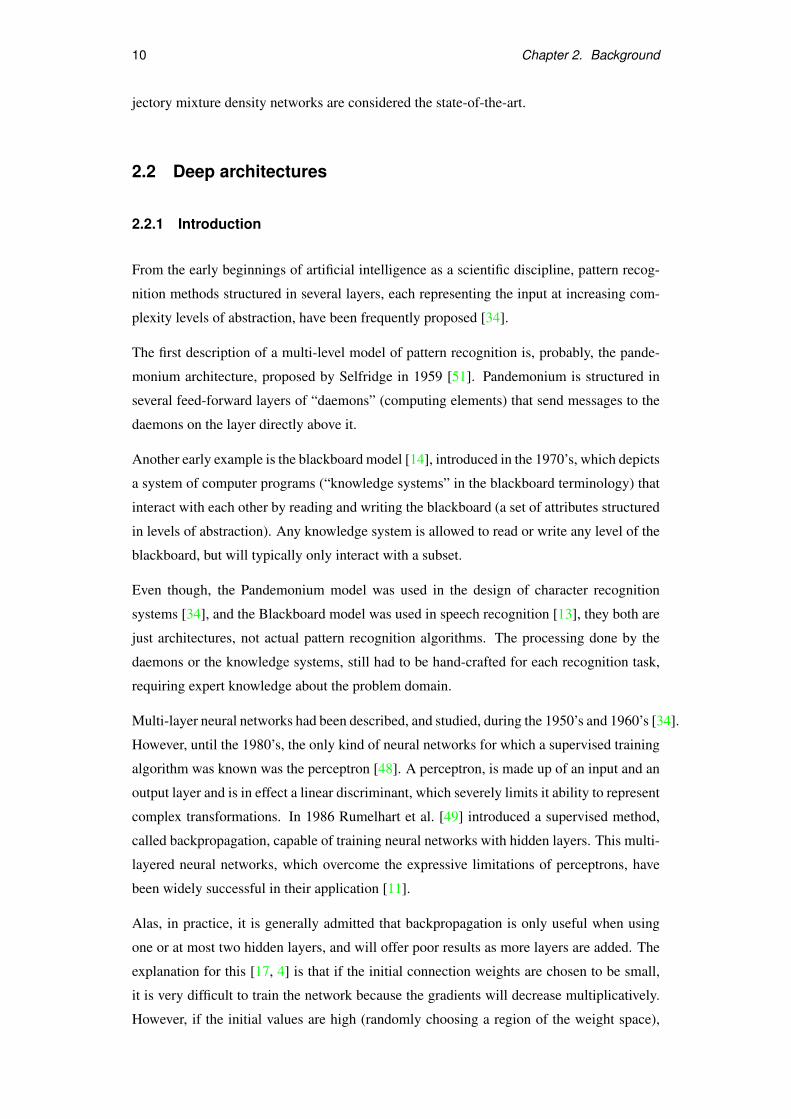
a mixture density network (MDN) [44], a methodology first proposed by Bishop [5]. A

MDN uses a ANN to calculate the parameters of the components of a mixture model (usu-

ally Gaussian), mapping the input to a (potentially multi-modal) probability distribution

(instead of a point) in the output space. The experimental setup is similar to the one used

for ANN. However, in this case 14 separate MDNs were trained (one for each dimension

of movement of seven articulators) using 2 Gaussians for the output density mixtures, each

Gaussian requiring a mixing factor, a mean and a variance. Although, Richmond’s initial

work obtained what, at the time, were state-of-the-art results of 1.42 mm average RMS error

on the MOCHA-TIMIT dataset, it did not use any dynamic constraints, just a low pass-filter

of the output to account for the slowly varying nature of articulator movement compared to

acoustic data.

In order to take into account the dynamic constraints of articulatory movements, a statistical

trajectory model can be used. These kind of models augment the output with dynamic (delta

and delta-delta) features and then use these position, velocity and acceleration estimation

series to calculate the most likely trajectory.

An example of a trajectory model is that proposed in 2008 by Zhang and Renals’ [56]:

a trajectory hidden Markov model using a two-stream HMM where acoustic recognition

and articulatory synthesis are modelled jointly. To perform inversion mapping with this

2.1. Previous approaches to articulatory inversion 9

Figure 2.3: Diagram of a mixture density network. Image courtesy of Korin Richmond.

system, first the state alignment for the appropriate HMM is derived from the acoustic

observation data. Then, the articulatory observation data is synthesised. In order to account

for the dynamic nature of the articulator’s positions the output is augmented with delta and

delta-delta features for each coordinate of each articulator. This delta-augmented estimation

is finally processed by a maximum likelihood parameter generator [54] that produces the

maximum likelihood trajectory of each articulator. Unfortunately, like Hiroya and Honda’s

HMM system. it requires the input of phonemic information added to the acoustic data to

obtain good results. using only the acoustic speech signal the system obtained an RMS error

of 1.705 mm on the MOCHA-TIMIT dataset.

Trajectory mixture density networks [45] (TMDNs) are an extension of Richmond’s previ-

ous work implementing a trajectory model. A TMDN is made up of MDNs trained trained

to output not only static (position), but also dynamic features (velocity and acceleration).

Then a maximum likelihood parameter generator algorithm (MLPG) is used to obtain the

maximum likelihood trajectory. This method was found to obtain better results than a static

MDN even if its output was low-pass filtered. It achieves an RMS error of 1.37 mm on the

MOCHA-TIMIT dataset and just 0.99 mm on the much more precise MNGU0 dataset1.

In 2010 Ling et al. [27] published an analysis of HMM-based articulatory inversion using

trajectory methods. They measured the accuracy of the system on the MNGU0 dataset,

obtaining an average RMS error of 1.076 mm when using only acoustic information as

input.

Unfortunately, several different EMA datasets were used to report the accuracy of the dif-

ferent methodologies, which makes it difficult to compare their performances. However,

MOCHA-TIMIT has been the most widely used EMA dataset, on which Richmond’s tra-

1The differences between these two datasets will be further explained in Chapter 3


jectory mixture density networks are considered the state-of-the-art.

2.2 Deep architectures

2.2.1 Introduction

From the early beginnings of artificial intelligence as a scientific discipline, pattern recog-

nition methods structured in several layers, each representing the input at increasing com-

plexity levels of abstraction, have been frequently proposed [34].

The first description of a multi-level model of pattern recognition is, probably, the pande-

monium architecture, proposed by Selfridge in 1959 [51]. Pandemonium is structured in

several feed-forward layers of “daemons” (computing elements) that send messages to the

daemons on the layer directly above it.

Another early example is the blackboard model [14], introduced in the 1970’s, which depicts

a system of computer programs (“knowledge systems” in the blackboard terminology) that

interact with each other by reading and writing the blackboard (a set of attributes structured

in levels of abstraction). Any knowledge system is allowed to read or write any level of the

blackboard, but will typically only interact with a subset.

Even though, the Pandemonium model was used in the design of character recognition

systems [34], and the Blackboard model was used in speech recognition [13], they both are

just architectures, not actual pattern recognition algorithms. The processing done by the

daemons or the knowledge systems, still had to be hand-crafted for each recognition task,

requiring expert knowledge about the problem domain.

Multi-layer neural networks had been described, and studied, during the 1950’s and 1960’s [34].

However, until the 1980’s, the only kind of neural networks for which a supervised training

algorithm was known was the perceptron [48]. A perceptron, is made up of an input and an

output layer and is in effect a linear discriminant, which severely limits it ability to represent

complex transformations. In 1986 Rumelhart et al. [49] introduced a supervised method,

called backpropagation, capable of training neural networks with hidden layers. This multi-

layered neural networks, which overcome the expressive limitations of perceptrons, have

been widely successful in their application [11].

Alas, in practice, it is generally admitted that backpropagation is only useful when using

one or at most two hidden layers, and will offer poor results as more layers are added. The

explanation for this [17, 4] is that if the initial connection weights are chosen to be small,

it is very difficult to train the network because the gradients will decrease multiplicatively.

However, if the initial values are high (randomly choosing a region of the weight space),

2.2. Deep architectures 11

v

h

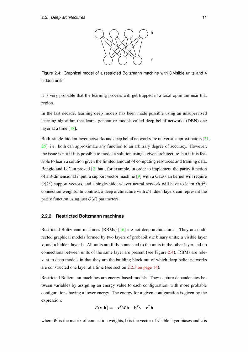
Figure 2.4: Graphical model of a restricted Boltzmann machine with 3 visible units and 4

hidden units.

it is very probable that the learning process will get trapped in a local optimum near that

region.

In the last decade, learning deep models has been made possible using an unsupervised

learning algorithm that learns generative models called deep belief networks (DBN) one

layer at a time [18].

Both, single-hidden-layer networks and deep belief networks are universal approximators [21,

25], i.e. both can approximate any function to an arbitrary degree of accuracy. However,

the issue is not if it is possible to model a solution using a given architecture, but if it is fea-

sible to learn a solution given the limited amount of computing resources and training data.

Bengio and LeCun proved [2]that , for example, in order to implement the parity function

of a d-dimensional input, a support vector machine [9] with a Gaussian kernel will require

O(2d) support vectors, and a single-hidden-layer neural network will have to learn O(d2)

connection weights. In contrast, a deep architecture with d-hidden layers can represent the

parity function using just O(d) parameters.

2.2.2 Restricted Boltzmann machines

Restricted Boltzmann machines (RBMs) [16] are not deep architectures. They are undi-

rected graphical models formed by two layers of probabilistic binary units: a visible layer

v, and a hidden layer h. All units are fully connected to the units in the other layer and no

connections between units of the same layer are present (see Figure 2.4). RBMs are rele-

vant to deep models in that they are the building block out of which deep belief networks

are constructed one layer at a time (see section 2.2.3 on page 14).

Restricted Boltzmann machines are energy-based models. They capture dependencies be-

tween variables by assigning an energy value to each configuration, with more probable

configurations having a lower energy. The energy for a given configuration is given by the

expression:

E(v,h) =−vTW h−bT v− cT h

where W is the matrix of connection weights, b is the vector of visible layer biases and c is


the vector of hidden layer biases.

The probability of a given configuration will be:

P(v,h) =1Z

e−E(v,h)

where Z = ∑v,h e−E(v,h)

Because no connections exist between units of the same layer, the probability of the units

in the top two layers factorize given the state of the other layer (i.e. the state of the units in

one layer are conditionally independent given the state of the units in the other layer), and

have the expression:

P(v j = 1 | h) = σ(−b j−Wj·h) (2.1)

P(h j = 1 | v) = σ(−c j−W T· j v) (2.2)

where, σ is the logistic sigmoid function σ(x) = 1(1+e−x) , W· j corresponds to the j-th column

of the weights matrix, and Wj· to the j-th row.

Sampling from the distribution modelled by the RBM can be done by performing Gibbs

sampling [8], initialising all units to arbitrary values and updating the two layers alternately

using equations 2.1 and 2.2.

RBMs can be used as associative memories. To sample from this memory, the state of some

of the units is clamped and Gibbs sampling is performed to obtain the state for the rest of

units.

Training an energy based model to capture a probability distribution is done by reducing the

energy of the more probable regions of the state space, and increasing the energy of the less

probable ones. “Shovelling” energy from regions of higher probability to regions of lower

probability [4].

Maximum likelihood learning in an RBM can be done using the following expressions [16]:

∆Wi j = 〈vih j〉0−〈vih j〉∞

∆bi = 〈vi〉0−〈vi〉∞

∆ci = 〈h1i 〉0−〈h1

i 〉∞

where:

• 〈·〉0 denotes the average when the visible units are clamped to the input values and

the hidden units are sampled from their conditional distribution (Equation 2.2).

• 〈·〉∞ denotes the average after assigning the input data to the visible units and running

Gibbs sampling until the stationary distribution is reached.


Unfortunately, maximum likelihood learning is too slow to be applied in a practical setting.

An alternative often used is contrastive divergence (CD) learning [16, 6] which uses the

following update rules for the weights and biases:

∆W 0i j ∝ 〈vih j〉0−〈vih j〉n

∆b0i ∝ 〈vi〉0−〈vi〉n

∆b1i ∝ 〈h1

i 〉0−〈h1i 〉n

where 〈·〉n denotes the average after assigning the input data to the visible units and per-

forming just n updates (as in Gibbs sampling) to each layer. Whereas in Gibbs sampling

the number of updates required to reach the stationary distribution can be very high, in con-

trastive divergence learning a very low number of updates is used, usually just 1. Contrastive

divergence has been empirically shown to work reasonably well [18]. Bengio’s "Learning

deep architectures for AI" [4] can be consulted for a tentative explanation of why it works.

2.2.2.1 Gaussian-Bernoulli RBM

For some kind of problems with real valued input features, having binary visible units is

not an appropriate representation of the data. An option is to normalize the value of the

input features to have magnitudes in the range [0,1] and use that value as the probability of

activation of the unit [4]. However, even this is not an appropriate representation in many

cases as the sampling introduces a lot of noise. An alternative that has received a lot of

attention in visual and acoustic data modelling is the use of Gaussian-Bernoulli RBMs [2].

In these kind of restricted Boltzmann machines, the value of visible units follows a Gaussian

activation probability and the hidden units are normal binary units that follow a Bernoulli

distribution.

In order to obtain simpler mathematical equations, the input data to Gaussian-Bernoulli

RBMs is usually normalized over the training dataset to have mean 0 and standard deviation

1 for each unit. In that case the energy of a given configuration is:

E(v,h) =12(v−b)T (v−b)−vTW h− cT h

and as in the standard RBM the conditional distribution of v given h factorizes with expres-

sion:

P(vj | h)∼N(−b j−Wj·h,1

)


...

v

h1

hn-1

hn

Figure 2.5: Graphical model of a deep belief network.

2.2.3 Deep belief networks

A deep belief network (DBN) [18] is a multi-layer generative probabilistic model, made up

of stochastic binary units organized in layers. The bottom layer is the visible layer v, while

the rest of the layers are hidden layers h1,h2, . . . ,hl .

In a DBN the top two layers (hl−1 and hl) are connected in an undirected manner and form

an RBM. The rest of layers are connected in a top-down directed fashion, see Figure 2.5.

The joint probability of a DBN factorizes as follows:

P(v,h1,h2, . . . ,hl) = P(v | h1)P(h1 | h2) . . .P(hl−2 | hl−1)P(hl−1,hl)

The probability of activation of a unit in any layer below the top two is conditionally inde-

pendent of the rest of units given the state of the layer directly on top of it, and follows the

expression:

P(hij | hi+1) = σ(−bi

j−W ij·h

i+1) (2.3)

Therefore, generating samples from a DBN can be achieved by doing Gibbs sampling of

the top two layers (i.e. alternately update h1−1 and h1 using equations (2.1) and (2.2) until

the stationary distribution is reached). Then, doing ancestral sampling of the lower layers

until we reach the visible layer using equation (2.3).

2.2.3.1 Training a deep belief network

The key to successfully train a DBN is to do it in a greedy, layer-wise manner [18]; adding

layers on top one at a time.


Initially, a DBN will consist of only 2 layers, the visible and the first hidden layer. These

initial two layers are connected in an undirected way (because they are the top two layers),

and trained as an RBM.

If a new layer is to be put on top, the connections between the previous top two layers

are transformed into directed top-down (directed from the hidden to the visible layer of the

RBM) connections. The new layer is added on top, connected to the previous top layer in

an undirected fashion. This new top two layers are, again, trained as an RBM. To obtain

the visible data of this new RBM, we must get samples from the previous top layer (now

visible layer of the top RBM) by running the data examples through the previous layers of

the DBN using equation23:

P(hlj | hl−1) = σ(−bl

j−W l−1· j

T hl−1)

2.2.3.2 Using a DBN for regression

As we have seen, a DBN is a generative model, it can not be used directly to perform

regression or classification. The purpose of creating a DBN if the aim is doing regression or

classification is to create a model capable of representing the visible data at different levels;

in the hope that higher layers will contain simpler representations of the data corresponding

to higher levels of abstraction. Therefore, obtaining features more useful for the purpose

of doing regression or classification. A trained DBN can be easily transformed into such a

regression or classification architecture.

There are several ways in which a DBN can be transformed into a classification architec-

ture. In this work, we are only interested in their use for regression. Hinton’s “A Practical

Guide to Training Restricted Boltzmann Machines” [15] can be consulted if the purpose is

classification.

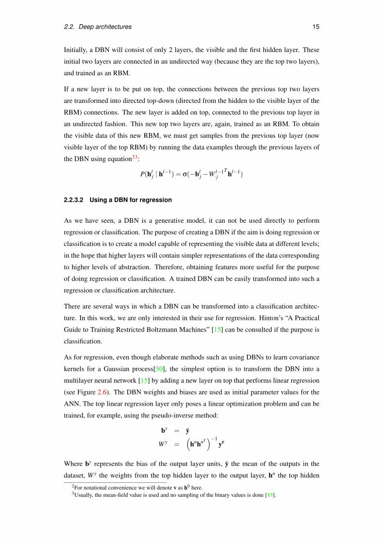
As for regression, even though elaborate methods such as using DBNs to learn covariance

kernels for a Gaussian process[50], the simplest option is to transform the DBN into a

multilayer neural network [15] by adding a new layer on top that performs linear regression

(see Figure 2.6). The DBN weights and biases are used as initial parameter values for the

ANN. The top linear regression layer only poses a linear optimization problem and can be

trained, for example, using the pseudo-inverse method:

by = y

W y =(

hnhnT)−1

yr

Where by represents the bias of the output layer units, y the mean of the outputs in the

dataset, W y the weights from the top hidden layer to the output layer, hn the top hidden2For notational convenience we will denote v as h0 here.3Usually, the mean-field value is used and no sampling of the binary values is done [15].


...

h

y

1

h n

v

Figure 2.6: DBN transformed into an regression ANN. Output y is calculated by performing

liner regression from the features in hn.

layer states for all datapoints in the dataset, and yr the mean-substracted outputs in the

dataset.

However, performance using the initial weights originated from a DBN, is usually not very

good. To improve its performance the model is fine-tuned by performing gradient descent;

generally, using the backpropagation algorithm.

Given that the model will have to be fine-tuned anyway, it may seem we have gained noth-

ing from creating the model from a DBN instead of creating an ANN with random initial

weights. However, empirical results show that an ANN with more than one or two layers

initialised with random weights is usually very difficult to train and tends to get stuck in un-

derperforming local optima. In contrast, ANN initialised with weights from a DBN usually

obtain better results [4].

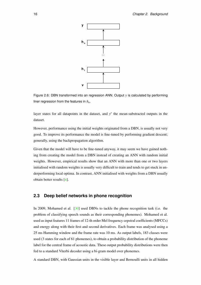
2.3 Deep belief networks in phone recognition

In 2009, Mohamed et al. [30] used DBNs to tackle the phone recognition task (i.e. the

problem of classifying speech sounds as their corresponding phonemes). Mohamed et al.

used as input features 11 frames of 12-th order Mel frequency cepstral coefficients (MFCCs)

and energy along with their first and second derivatives. Each frame was analysed using a

25 ms Hamming window and the frame rate was 10 ms. As output labels, 183 classes were

used (3 states for each of 61 phonemes), to obtain a probability distribution of the phoneme

label for the central frame of acoustic data. These output probability distributions were then

fed to a standard Viterbi decoder using a bi-gram model over phonemes.

A standard DBN, with Gaussian units in the visible layer and Bernoulli units in all hidden

2.3. Deep belief networks in phone recognition 17

... ...

x

h

y

1

h ny

x

h 1

h n

h n+1

BP-DBN AM-DBN

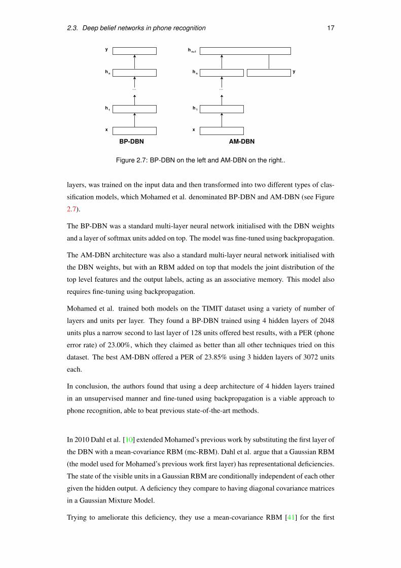
Figure 2.7: BP-DBN on the left and AM-DBN on the right..

layers, was trained on the input data and then transformed into two different types of clas-

sification models, which Mohamed et al. denominated BP-DBN and AM-DBN (see Figure

2.7).

The BP-DBN was a standard multi-layer neural network initialised with the DBN weights

and a layer of softmax units added on top. The model was fine-tuned using backpropagation.

The AM-DBN architecture was also a standard multi-layer neural network initialised with

the DBN weights, but with an RBM added on top that models the joint distribution of the

top level features and the output labels, acting as an associative memory. This model also

requires fine-tuning using backpropagation.

Mohamed et al. trained both models on the TIMIT dataset using a variety of number of

layers and units per layer. They found a BP-DBN trained using 4 hidden layers of 2048

units plus a narrow second to last layer of 128 units offered best results, with a PER (phone

error rate) of 23.00%, which they claimed as better than all other techniques tried on this

dataset. The best AM-DBN offered a PER of 23.85% using 3 hidden layers of 3072 units

each.

In conclusion, the authors found that using a deep architecture of 4 hidden layers trained

in an unsupervised manner and fine-tuned using backpropagation is a viable approach to

phone recognition, able to beat previous state-of-the-art methods.

In 2010 Dahl et al. [10] extended Mohamed’s previous work by substituting the first layer of

the DBN with a mean-covariance RBM (mc-RBM). Dahl et al. argue that a Gaussian RBM

(the model used for Mohamed’s previous work first layer) has representational deficiencies.

The state of the visible units in a Gaussian RBM are conditionally independent of each other

given the hidden output. A deficiency they compare to having diagonal covariance matrices

in a Gaussian Mixture Model.

Trying to ameliorate this deficiency, they use a mean-covariance RBM [41] for the first


layer of their system. A mean-covariance RBM is made-up of a set of Gaussian units (also

called mean units) and another set of units called the precision units. The precision units

form a third order Boltzmann machine, and define a sample-specific covariance matrix by

capturing multiplicative interactions between two visible units and one precision unit.

The output of this mc-RBM was used as the input to a DBN. No backpropagation is done

to the mc-RBM when the system is transformed into an ANN after unsupervised training.

The acoustic features used as input in this paper differ from Mohamed’s previous work:

15 acoustic frames each formed by 39 Mel scale filterbank coefficients and 1 energy log

magnitudes were concatenated and PCA whitening applied, after which only the 384 most

important components were used as inputs. Of special relevance is the absence of delta

features, which purportedly are not needed when using an mc-RBM.

Best results, measured on the TIMIT test dataset, were achieved using 1024 precision units

and 512 mean units for the mc-RBM, and 8 more hidden layers of 2048 units each; obtaining

a phone error rate of 21.7%.

Dahl et al. report training a system equivalent to that of Mohamed’s previous work but

with an mc-RBM as the first layer in order to “isolate the advantage of using an mc-RBM

instead of a Gaussian-RBM” from the improvement due to the new kind of inputs. They

obtained a phone error rate of 22.3% (a 1.4% improvement with respect to Mohamed’s

work). However no details about the configuration are reported in the paper. Of special

interest would be whether they utilized delta features as inputs, as they consider the ability

of the mc-RBM to “extract its own useful features that make explicit inclusion of difference

features unnecessary” the main advantage of its use. Therefore, if they were not used, the

improvement would be more indicative of the advantage of using first layer an mc-RBM

instead of a Gaussian-RBM for the first layer.

It must be kept in mind that Dahl et al. report that using an mc-RBM more than doubled

the training time of the system. Dahl et al. have abandoned the use of mc-RBM in their

more recent publications. Whether this is because their accuracy improvement disappears

when adding other modifications or because they result impractical due to their long train-

ing times has not been specified.

In 2011, Mohamed et al. published [31] a review of their previous work. In this paper they

introduce the use of filterbank coefficients augmented with delta and delta-delta features (a

simpler representation than Mel frequency cepstral coefficients). They obtain a phone error

rate of 20.7% on the TIMIT test dataset, and conclude that a deep architecture is able to

extract better features out of these less processed input features.

2.3. Deep belief networks in phone recognition 19

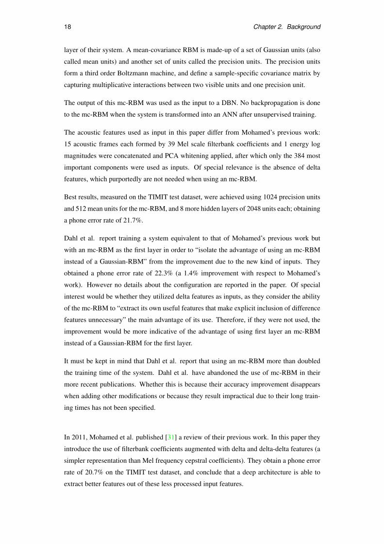
Figure 2.8: On the left forty random features learned by the first layer RBM in Jaitly and

Hinton [22](each features is shown by plotting the connection weights from a hidden unit

to all visible units). On the right the Fourier transform of the features. (Image reproduced

from [22] with the author’s permission)

In 2011, Mohamed et al. [32] published an extension of Mohamed’s previous work. In this

work, they compare their previous results using Mel frequency cepstral coefficients with

three modification: (1) the use of a vector of 40 linear discriminant analysis features (LDA),

(2) the combination of LDA features using speaker adaptation by vocal tract length normal-

isation, and (3) the addition of discriminative features trained using the boosted maximum

mutual information criterion [37].

As in previous papers, the performance is measured on the test TIMIT dataset. Raw LDA

features were found to offer no accuracy improvement. However, both speaker adaptation

and discriminative features offered improved results. A 4 hidden-layers ANN pretrained as

a DBN, with 1024 units per hidden layer using as inputs LDA features after speaker adapta-

tions obtained a phone recognition error of 20.3%. Adding discriminative features reduced

the error even further to 19.6%.

In 2011, Jaitly and Hinton [22] introduced the use of an specialized type of RBMs to model

speech data directly from the raw acoustic signal, instead of using a low dimensional en-

coding as filterbank coefficients, Mel cepstrum coefficients or linear predictive coding.

In their work, Jaitly and Hinton, use as the first layer of their system an RBM that has Gaus-

sian visible units and rectified linear hidden units (RLU). The value of a rectified linear unit

is max(0,N(x,σ(x)) where x represents the input to the unit. This kind of units where first

used by Nair and Hinton and are reported to improve the performance of DBN based sys-

tems in comparison with other kinds of continuously valued hidden units (like for example

Gaussian units).

Jaitly and Hinton, trained this kind of RBM on the TIMIT development dataset raw input

signal and found it captured features like those shown in Figure 2.8.


Finally, they trained a standard 3 hidden layers (4000 units each) DBN using these features

as input, and use it for phone recognition using 183 states as in Mohamed’s work. They

obtain a phone error rate on the TIMIT test dataset of 21.8%. A remarkable result given

that they use the raw acoustic signal as input.

The good results obtained by deep belief network systems in phone recognition led us to

hypothesise they could be a good system for articulatory inversion. The similarity is ob-

vious, both problems process acoustic speech signals. However, there is a very important

difference between both: phone recognition is a classification problem, while articulatory

inversion is a regression problem.

Chapter 3

Data and Evaluation Criteria

3.1 The MNGU0 dataset

Although the FSEW0 dataset (part of the MOCHA-TIMIT corpus [55]) has been the elec-

tromagnetic midsagittal articulography dataset most widely used in previous articulatory

inversion research, in this dissertation we have opted for using the recently introduced

MNGU0 dataset [47]. Our preference for the MNGU0 dataset is based on several issues

concerning the quality of the MOCHA-TIMIT EMA measurements.

MOCHA-TIMIT is an older dataset and was recorded using a Cartsens AG200 electromag-

netic articulograph. This articulograph consists of only 3 fixed transmitter coils. These

make it possible to measure the position of the transducer coils only on a 2-dimensional

plane. Therefore, movement of the head during a EMA recording session or rotation of the

transducer coils due to articulator movement can have a negative impact on the precision of

the measurements. Moreover, during the recording of the MOCHA-TIMIT fsew0 dataset, a

coil became detached and had to be re-attached; since it is impossible to attach it at exactly

the same position, inevitably this also added a certain degree of inconsistency to the dataset.

In contrast, the MNGU0 [46] dataset was recorded using a more modern Cartsens AG500

electromagnetic articulograph. This newer model consists of 6 transmitter coils, which

make it possible to track the position of the transducer coils in three dimensions along

with two angles of rotation. This makes movement of the head during the EMA session

irrelevant, as the articulator positions are calculated relative to the position of other reference

coils placed on the skull. Moreover, no coil became detached during the recording of the

MNGU0 dataset.

To show that the MNGU0 dataset has a higher level of precision than the FSEW0 dataset,

Richmond [46] measured the accuracy of his trajectory mixture density network articulatory

inversion system on both, obtaining an RMSE of 1.54mm for FSEW0 and 0.99mm for

21

22 Chapter 3. Data and Evaluation Criteria

T3T2T1

UL

LL

LI

Figure 3.1: Midsagittal plane figure showing the positioning of electromagnetic coils for vocal

tract articulator tracking in the MNGU0 dataset. The articulators tracked are: upper lip (UL),

lower lip (LL), lower incisor (LI), tongue tip (T1), tongue blade (T2), and tongue dorsum (T3).

Image courtesy of Korin Richmond.

MNGU0.

3.1.1 Data setup

The MNGU0 EMA dataset used in this dissertation, consists of 1263 utterances recorded

from a single speaker in a single session. Parallel recordings of acoustic data and the po-

sition of 6 coils is available. Transducer coils were placed in the midsagittal plane at the

upper lip, lower lip, lower incisors, tongue tip, tongue blade and tongue dorsum (see Figure

3.1).

Although MNGU0 EMA data consists of 3-dimensional measurements, only movement

in the midsagittal plane (therefore 2-dimensional) was considered. The reason for this is

twofold, movement perpendicular to the midsagittal plane was very small, and it eases com-

parison with results from previous research by Richmond [46].

Each EMA data frame is made up by 12 coordinates, two (x and y position) for each articu-

lator tracked, with a sampling frequency of 200 Hz. The acoustic data consists on frames of

40 frequency warped line spectral frequencies (LSFs) [52] and a gain value, the frame shift

step is 5 ms in order to obtain acoustic features at the same frequency as the EMA data.

In our experiments we will use the same data setup as Richmond in [46]. As input, we use

a context window of 10 acoustic frames selecting only every other frame. Therefore, each

input window will span a period of 100 ms. As output, we will use the EMA frame that

corresponds to the time at the middle of the current acoustic window, i.e. between acoustic

3.2. Evaluation criteria 23

frames 5 and 6.

The dataset is partitioned in three sets: a validation and a training set comprising 63 utter-

ances each, and a training set consisting of the other 1137 utterances.

3.2 Evaluation criteria

In this work, we will use two metrics to measure the accuracy of our system:

• The root mean-squared error (RMSE), this is the most widely used measure of an

articulatory inversion system performance, and is defined as

RMSE =

√1N ∑

i(ei− ti)2

where ei is the estimated tract variable and ti the actual tract variable at time i.

• The correlation with the actual articulator trajectories, defined as

r =∑i(ei− e)(ti− t)√

∑i(ei− e)2 ∑i(ti− t)2

where e is the mean value of the estimated tract variable, t the mean value of the

actual tract variable.

A good articulatory inversion system must obtain low RMSE and high correlation with

respect to real articulatory data.

We will focus on the root mean-squared error as it is the most widely reported measure of

articulatory inversion accuracy and is the only measure for which we have previous results

on the MNGU0 dataset. However, we will also report the correlation of the most important

results.

3.3 Benchmarks

In order to judge the relevance of our results, we need to set some reference points with

which we can compare them using the test set of the MNGU0 dataset.

A linear model that uses as input a window of acoustic data and as output a frame of artic-

ulatory data, obtains an average RMSE of 1.52 mm. This result gives us an idea of what

can be achieved with a very simple model. Any RMSE greater than that would indicate our

system is obtaining very bad results.

A regular one-hidden-layer artificial neural network with 300 units, obtains an average

RMSE of about 1.13 mm. this sets a benchmark for a simple model but one not so naive as

a linear model.

24 Chapter 3. Data and Evaluation Criteria

Then we can set some reference points for what would be state-of-the-art accuracies. Rich-

mond’s trajectory mixture density networks1 obtain when using one Gaussian-mixture per

articulatory channel an average RMSE of 1.03 mm. When using 1,2 or 4 Gaussian-mixtures

(the number is optimized for each channel) the average RMSE shrinks to 0.99 mm [46].

Recently, Richmond’s trajectory mixture density network have obtained a new, still unpub-

lished, record accuracy of 0.96 mm RMSE [43].

We cannot know how much variability is due to measurement error of the EMA machine.

Moreover, because not all articulators are equally relevant in the production of a given

sound [35], a slight change of position of some of them will not affect the sound produced

much, this also introduces a certain degree of variability in the articulatory data that is

inherent to the speech production process and cannot be avoided. Therefore, it is impossible

for us to know what is the smallest RMS error achievable.

1We consider Richmond’s TMDN as the state-of-the-art given that he obtains the best accuracies on theMOCHA-TIMIT , which is the most widely tried EMA dataset. Fortunately, we also have results for the novelMNGU0 dataset.

Chapter 4

Implementation and Results

Motivated by their good performance in phone recognition, we introduce in this dissertation

a deep belief network for articulatory inversion.

Given that the process of training restricted Boltzmann machines is computationally expen-

sive, we designed our system to take advantage of the computational speed-up provided by

GP-GPU (general purpose computation on graphics processing units). In our implementa-

tion we used the matrix algebra CUDAMat Python library [29]. We obtained approximately

5 times shorter RBM training times and 2.5 times shorter backpropagation times compared

to using 6 CPUs. More details about our specific hardware configuration and training times

can be found in Appendix A.

4.1 A deep belief network for articulatory inversion

4.1.1 Pretraining

To create our articulatory inversion system, first we trained a deep belief network to model

speech acoustic data1. Given that acoustic data is not binary, but continuous, we used a

Gaussian-Bernoulli restricted Boltzmann machine (see page 13) for the first layer of our

DBN. To train it we used the contrastive divergence criterion using, as it is common, just 1

sampling step2 (CD1).

The final training configuration parameters are shown in table 4.1, and were the result of

manually tuning them to obtain a low reconstruction error. The heuristics in Hinton’s “A

1To be more precise speech acoustic data produced by the speaker in the MNGU0 dataset.2A better generative model is usually obtained using a higher number of sampling steps [4]. However, it is

considered not worth it to use a higher number of steps [15] when the model is going to be transformed into anartificial neural network and fine-tuned with backpropagation.

25

26 Chapter 4. Implementation and Results

Parameter Value

Learning rate 0.00001

Momentum 0.5 (10 first epochs) 0.9 (rest of epochs)

Total epochs 200

Minibatch size 100

Initial weights N (0, 0.01)

Initial visible bias 0

Initial hidden bias −4

Weight decay 0.0001

Table 4.1: Training configuration for the Gaussian-Bernoulli RBM used as the first layer of

the articulatory inversion DBN.

practical guide to training restricted Boltzmann machines” [15] were of great help in this

endeavour.

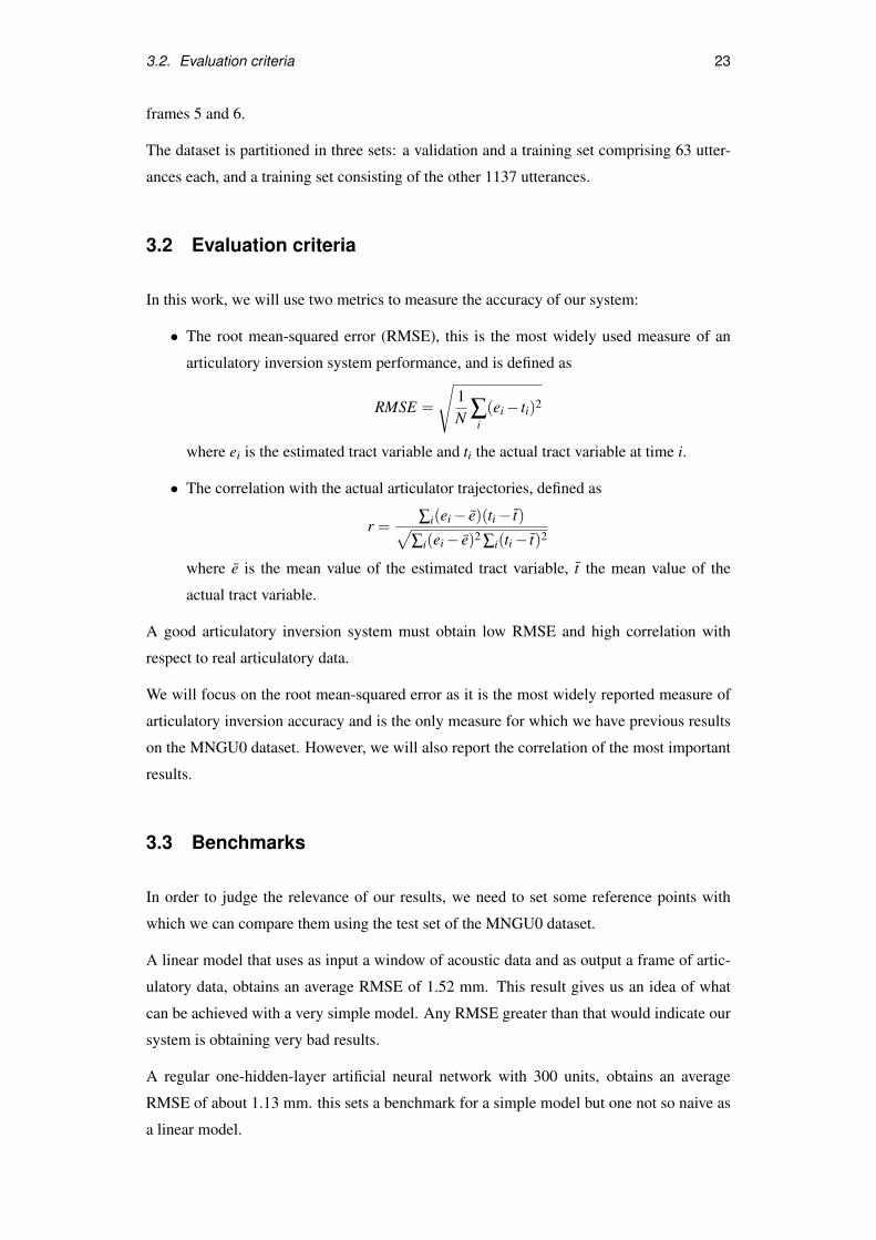
Figure 4.1 shows some of the receptive fields learned by sixty hidden units of the Gaussian-

Bernoulli RBM.

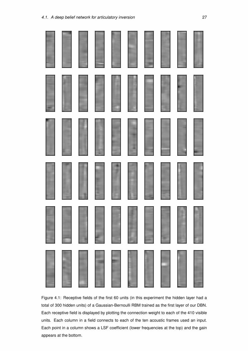
We can observe some of them show blobs of high or low activation (light and dark regions

respectively), this blobs capture continuity patterns of the acoustic data in the time and

frequency domains. Four examples can be seen in Figure 4.2 on page 28.

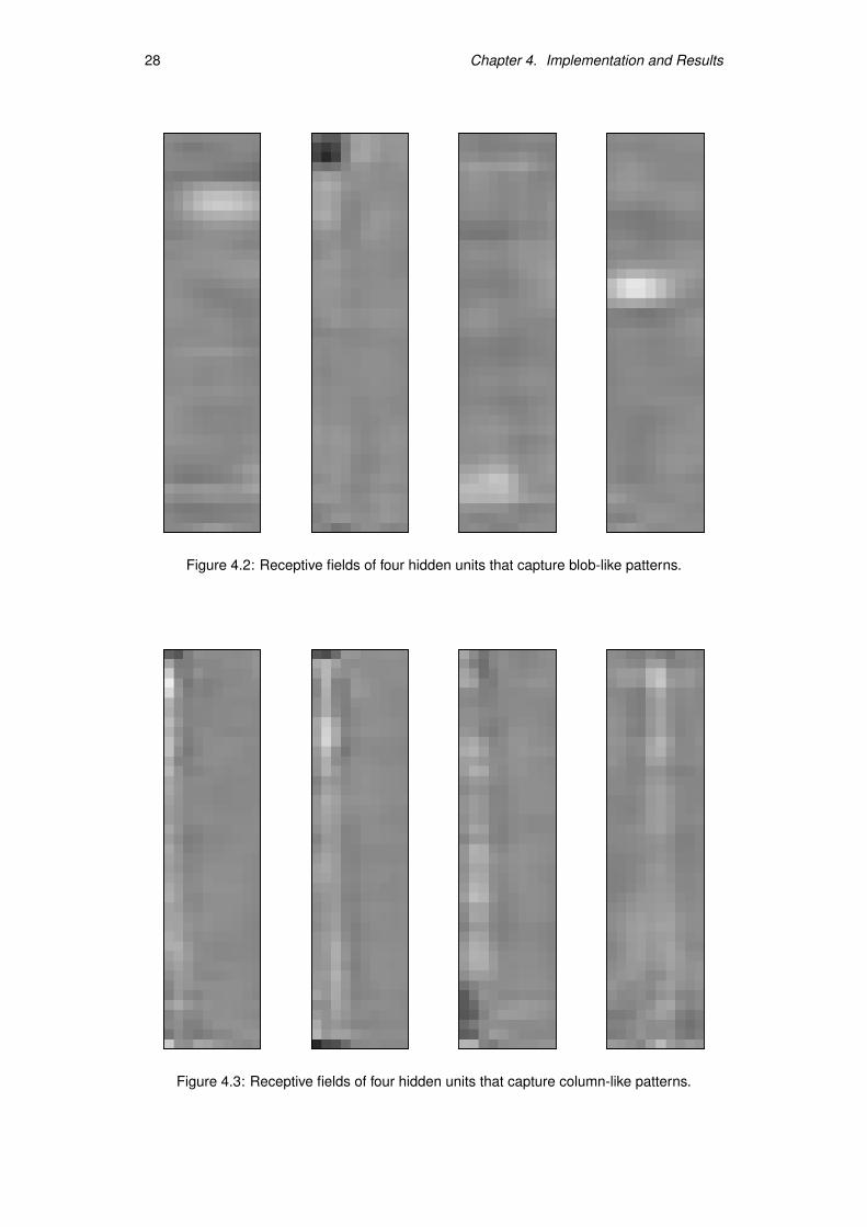
Some other units, display vertical patterns of high activity flanked by low activity (light ver-

tical lines flanked by dark vertical lines) and usually occupy the whole frequency (vertical)

spectrum. These features capture activation contrasts between contiguous acoustic frames.

Four examples can be seen in Figure 4.3.

We tried different sizes for the hidden layer of the Gaussian-Bernoulli RBM. We found that

the final average reconstruction error decreases as the number of hidden units is increased,

but saturates at 300 units and does not improve by adding more hidden units after that.

More layers were trained on top by following the conventional procedure for DBNs: freez-

ing the weights of the layer just trained and using its hidden layer activation probabilities as

input for the new layer. In these higher layers both visible and hidden units take binary val-

ues3 and are therefore Bernoulli-Bernoulli RBMs. The training configuration for the higher

layers is shown in Table 4.2 on page 29.

3However, no sampling is performed of the input, it is the activation probability that is used as input for thenew visible layer.

4.1. A deep belief network for articulatory inversion 27

Figure 4.1: Receptive fields of the first 60 units (in this experiment the hidden layer had a

total of 300 hidden units) of a Gaussian-Bernoulli RBM trained as the first layer of our DBN.

Each receptive field is displayed by plotting the connection weight to each of the 410 visible

units. Each column in a field connects to each of the ten acoustic frames used an input.

Each point in a column shows a LSF coefficient (lower frequencies at the top) and the gain

appears at the bottom.


Figure 4.2: Receptive fields of four hidden units that capture blob-like patterns.

Figure 4.3: Receptive fields of four hidden units that capture column-like patterns.


Parameter Value



Total epochs 200

Minibatch size 100

Initial weights N (0, 0.01)

Initial visible bias 0

Initial hidden bias −4

Weight decay 0.0001

Table 4.2: Training configuration for the Bernoulli-Bernoulli RBMs used for all layers of the

articulatory inversion DBN except the first.

...

h1

h n-1

v

y

h n

...

h1

h n-1

v

h n

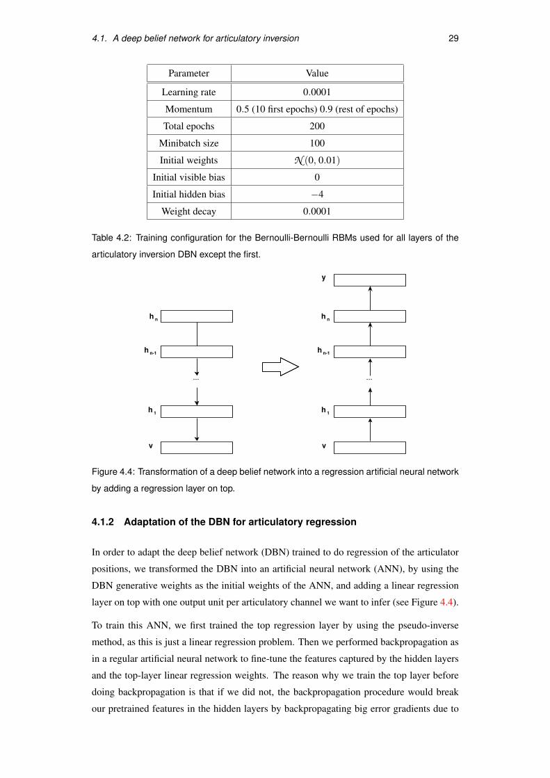
Figure 4.4: Transformation of a deep belief network into a regression artificial neural network

by adding a regression layer on top.

4.1.2 Adaptation of the DBN for articulatory regression

In order to adapt the deep belief network (DBN) trained to do regression of the articulator

positions, we transformed the DBN into an artificial neural network (ANN), by using the

DBN generative weights as the initial weights of the ANN, and adding a linear regression

layer on top with one output unit per articulatory channel we want to infer (see Figure 4.4).

To train this ANN, we first trained the top regression layer by using the pseudo-inverse

method, as this is just a linear regression problem. Then we performed backpropagation as

in a regular artificial neural network to fine-tune the features captured by the hidden layers

and the top-layer linear regression weights. The reason why we train the top layer before

doing backpropagation is that if we did not, the backpropagation procedure would break

our pretrained features in the hidden layers by backpropagating big error gradients due to


Parameter Value



Total epochs 150

Minibatch size 100

Weight decay 0.0001

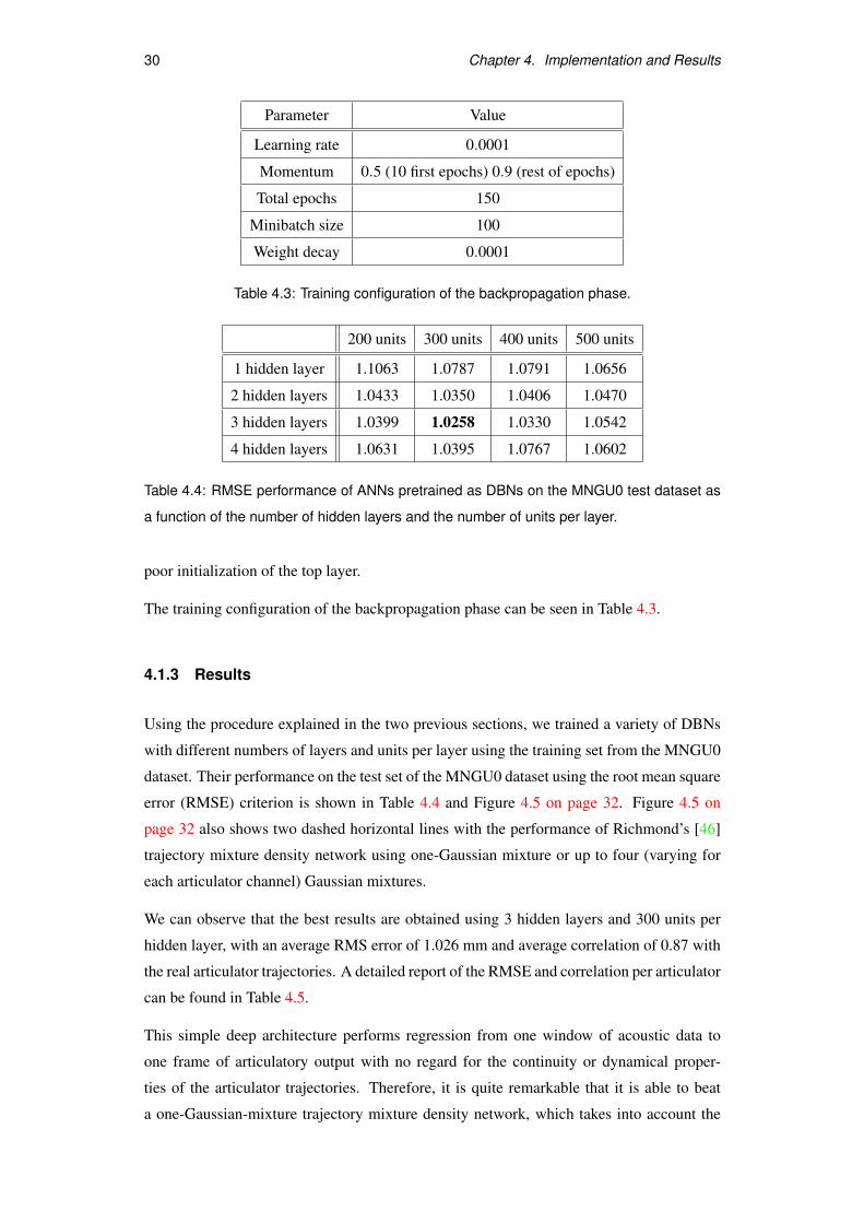
Table 4.3: Training configuration of the backpropagation phase.

200 units 300 units 400 units 500 units

1 hidden layer 1.1063 1.0787 1.0791 1.0656

2 hidden layers 1.0433 1.0350 1.0406 1.0470

3 hidden layers 1.0399 1.0258 1.0330 1.0542

4 hidden layers 1.0631 1.0395 1.0767 1.0602

Table 4.4: RMSE performance of ANNs pretrained as DBNs on the MNGU0 test dataset as

a function of the number of hidden layers and the number of units per layer.

poor initialization of the top layer.

The training configuration of the backpropagation phase can be seen in Table 4.3.

4.1.3 Results

Using the procedure explained in the two previous sections, we trained a variety of DBNs

with different numbers of layers and units per layer using the training set from the MNGU0

dataset. Their performance on the test set of the MNGU0 dataset using the root mean square

error (RMSE) criterion is shown in Table 4.4 and Figure 4.5 on page 32. Figure 4.5 on

page 32 also shows two dashed horizontal lines with the performance of Richmond’s [46]

trajectory mixture density network using one-Gaussian mixture or up to four (varying for

each articulator channel) Gaussian mixtures.

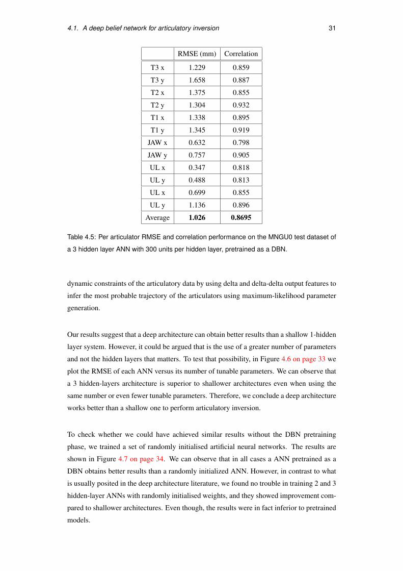
We can observe that the best results are obtained using 3 hidden layers and 300 units per

hidden layer, with an average RMS error of 1.026 mm and average correlation of 0.87 with

the real articulator trajectories. A detailed report of the RMSE and correlation per articulator

can be found in Table 4.5.

This simple deep architecture performs regression from one window of acoustic data to

one frame of articulatory output with no regard for the continuity or dynamical proper-

ties of the articulator trajectories. Therefore, it is quite remarkable that it is able to beat

a one-Gaussian-mixture trajectory mixture density network, which takes into account the


RMSE (mm) Correlation

T3 x 1.229 0.859

T3 y 1.658 0.887

T2 x 1.375 0.855

T2 y 1.304 0.932

T1 x 1.338 0.895

T1 y 1.345 0.919

JAW x 0.632 0.798

JAW y 0.757 0.905

UL x 0.347 0.818

UL y 0.488 0.813

UL x 0.699 0.855

UL y 1.136 0.896

Average 1.026 0.8695

Table 4.5: Per articulator RMSE and correlation performance on the MNGU0 test dataset of

a 3 hidden layer ANN with 300 units per hidden layer, pretrained as a DBN.

dynamic constraints of the articulatory data by using delta and delta-delta output features to

infer the most probable trajectory of the articulators using maximum-likelihood parameter

generation.

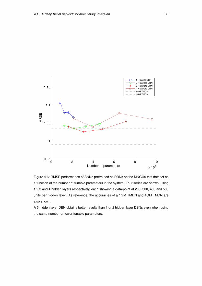
Our results suggest that a deep architecture can obtain better results than a shallow 1-hidden

layer system. However, it could be argued that is the use of a greater number of parameters

and not the hidden layers that matters. To test that possibility, in Figure 4.6 on page 33 we

plot the RMSE of each ANN versus its number of tunable parameters. We can observe that

a 3 hidden-layers architecture is superior to shallower architectures even when using the

same number or even fewer tunable parameters. Therefore, we conclude a deep architecture

works better than a shallow one to perform articulatory inversion.

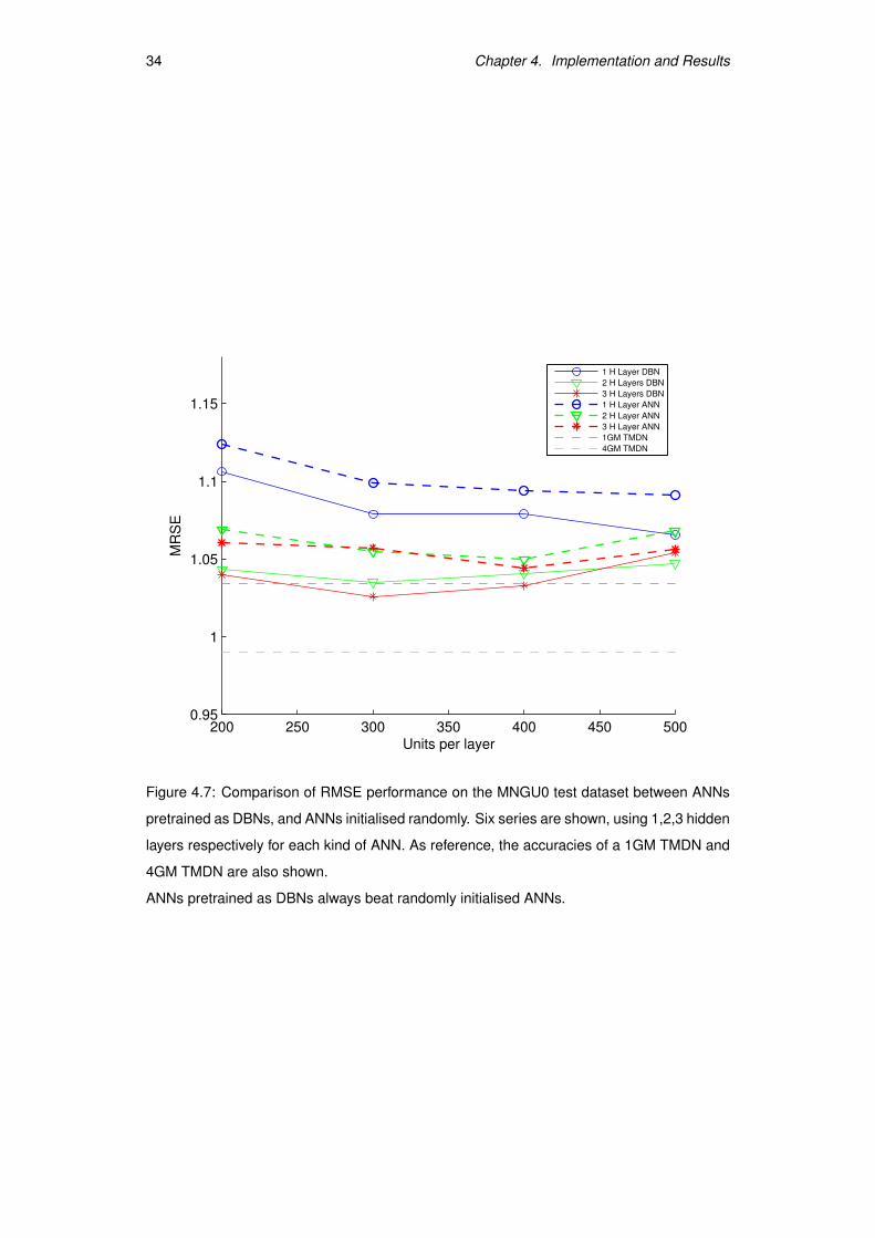
To check whether we could have achieved similar results without the DBN pretraining

phase, we trained a set of randomly initialised artificial neural networks. The results are

shown in Figure 4.7 on page 34. We can observe that in all cases a ANN pretrained as a

DBN obtains better results than a randomly initialized ANN. However, in contrast to what

is usually posited in the deep architecture literature, we found no trouble in training 2 and 3

hidden-layer ANNs with randomly initialised weights, and they showed improvement com-

pared to shallower architectures. Even though, the results were in fact inferior to pretrained

models.


200 250 300 350 400 450 5000.95

1

1.05

1.1

1.15

MR

SE

Units per layer

1 H Layer DBN

2 H Layers DBN

3 H Layers DBN

4 H Layers DBN

1GM TMDN

4GM TMDN

Figure 4.5: RMSE performance of ANNs pretrained as DBNs on the MNGU0 test dataset as

a function of the number of units per layer. Four series are shown, using 1,2,3 and 4 hidden

layers respectively. As reference, the accuracies of a 1GM TMDN and 4GM TMDN are also

shown.

Best results are obtained using a 3 hidden layers DBN with 300 units per hidden layer.


0 2 4 6 8 10

x 105

0.95

1

1.05

1.1

1.15

MR

SE

Number of parameters

1 H Layer DBN

2 H Layers DBN

3 H Layers DBN

4 H Layers DBN

1GM TMDN

4GM TMDN


a function of the number of tunable parameters in the system. Four series are shown, using

1,2,3 and 4 hidden layers respectively, each showing a data-point at 200, 300, 400 and 500

units per hidden layer. As reference, the accuracies of a 1GM TMDN and 4GM TMDN are

also shown.

A 3 hidden layer DBN obtains better results than 1 or 2 hidden layer DBNs even when using

the same number or fewer tunable parameters.


200 250 300 350 400 450 5000.95

1

1.05

1.1

1.15

MR

SE

Units per layer

1 H Layer DBN

2 H Layers DBN

3 H Layers DBN

1 H Layer ANN

2 H Layer ANN

3 H Layer ANN

1GM TMDN

4GM TMDN

Figure 4.7: Comparison of RMSE performance on the MNGU0 test dataset between ANNs

pretrained as DBNs, and ANNs initialised randomly. Six series are shown, using 1,2,3 hidden

layers respectively for each kind of ANN. As reference, the accuracies of a 1GM TMDN and

4GM TMDN are also shown.

ANNs pretrained as DBNs always beat randomly initialised ANNs.

4.2. Low-pass filtering 35

T3 x T3 y T2 x T2 y T1 x T1 y JAW x JAW y UL x UL y LL x LL y

7 Hz 6 Hz 7 Hz 8 Hz 7 Hz 9 Hz 6 Hz 9 Hz 6 Hz 6 Hz 7 Hz 10 Hz

Table 4.6: List of optimal integer cut-off frequency for each articulator channel

4.2 Low-pass filtering

So far in our system each frame of articulatory data is inferred from a window of acous-

tic data with no regard for the fact that the articulatory data forms a time series and will

have some dynamical characteristics. In Richmond’s recent work, dynamical constraints are

added by inferring delta and delta-delta (velocity and acceleration) features along with the

static estimation of the articulator’s position. Using these static and dynamic features Rich-

mond runs a maximum likelihood parameter generation (MLPG) that infers the most likely

trajectory in conformance with the dynamic constraints [45]. Unfortunately, the MLPG

algorithm requires probability distributions of the static and dynamic features, not point es-

timations, and due to the limited time we had for this dissertation, we considered it out of

reach.

In order to account for the dynamic nature of articulatory data in a simpler manner, we can

take the approach followed by Richmond in his earlier work. In his doctoral dissertation,

Richmond noticed the output of his articulatory inversion system based on artificial neural

networks had a higher variability (higher frequency components) than real articulatory data.

To eliminate the higher frequency components of his output, Richmond applied a low-pass

filter obtaining as a result articulatory trajectory estimations with a lower root mean square

error and higher correlation.

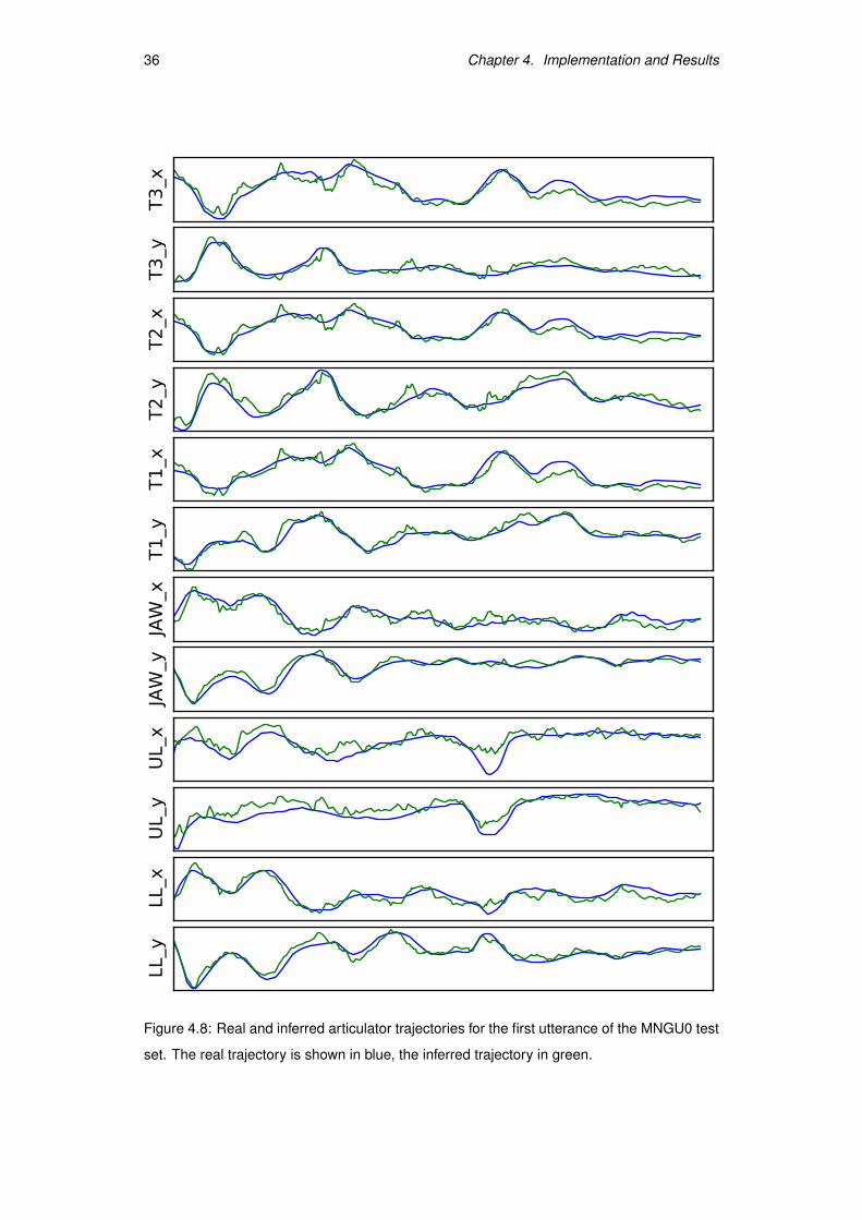
If we plot the output of our system, for example for the first utterance in the MNGU0 test

set as shown in Figure 4.8 on the following page, we can observe our output also has high

frequency components that appear absent in the real articulatory data.

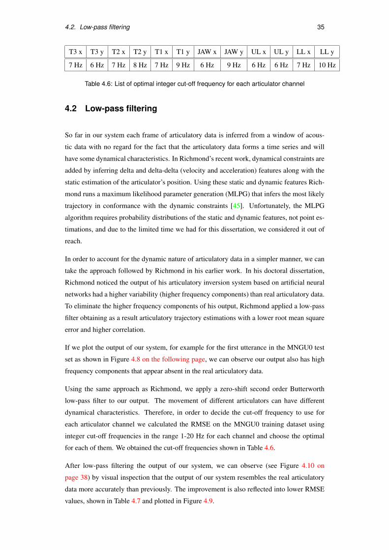
Using the same approach as Richmond, we apply a zero-shift second order Butterworth

low-pass filter to our output. The movement of different articulators can have different

dynamical characteristics. Therefore, in order to decide the cut-off frequency to use for

each articulator channel we calculated the RMSE on the MNGU0 training dataset using

integer cut-off frequencies in the range 1-20 Hz for each channel and choose the optimal

for each of them. We obtained the cut-off frequencies shown in Table 4.6.

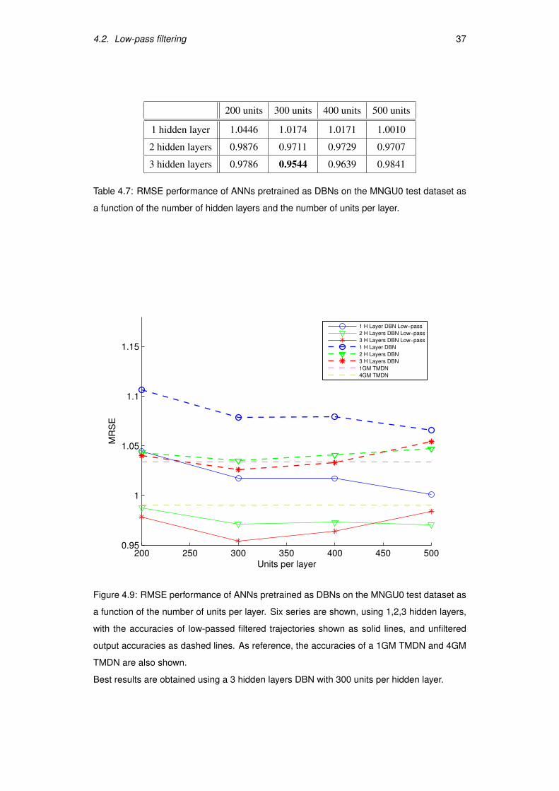
After low-pass filtering the output of our system, we can observe (see Figure 4.10 on

page 38) by visual inspection that the output of our system resembles the real articulatory

data more accurately than previously. The improvement is also reflected into lower RMSE

values, shown in Table 4.7 and plotted in Figure 4.9.


T3_x

T3_y

T2_x

T2_y

T1_x

T1_y

JAW_x

JAW_y

UL_x

UL_y

LL_x

LL_y

Figure 4.8: Real and inferred articulator trajectories for the first utterance of the MNGU0 test

set. The real trajectory is shown in blue, the inferred trajectory in green.

4.2. Low-pass filtering 37

200 units 300 units 400 units 500 units

1 hidden layer 1.0446 1.0174 1.0171 1.0010

2 hidden layers 0.9876 0.9711 0.9729 0.9707

3 hidden layers 0.9786 0.9544 0.9639 0.9841

Table 4.7: RMSE performance of ANNs pretrained as DBNs on the MNGU0 test dataset as

a function of the number of hidden layers and the number of units per layer.

200 250 300 350 400 450 5000.95

1

1.05

1.1

1.15

MR

SE

Units per layer

1 H Layer DBN Low−pass

2 H Layers DBN Low−pass


1 H Layer DBN

2 H Layers DBN

3 H Layers DBN

1GM TMDN

4GM TMDN


a function of the number of units per layer. Six series are shown, using 1,2,3 hidden layers,

with the accuracies of low-passed filtered trajectories shown as solid lines, and unfiltered

output accuracies as dashed lines. As reference, the accuracies of a 1GM TMDN and 4GM

TMDN are also shown.

Best results are obtained using a 3 hidden layers DBN with 300 units per hidden layer.


T3_x

T3_y

T2_x

T2_y

T1_x

T1_y

JAW_x

JAW_y

UL_x

UL_y

LL_x

LL_y

Figure 4.10: Real and inferred articulator trajectories for the first utterance of the MNGU0 test

set. The inferred trajectory has been low-pass filtered using the cut-off frequencies shown in

Table 4.6.The real trajectory is shown in blue, the inferred trajectory in green.

4.3. Output augmentation, multitask learning 39


T3 x 1.143 0.877

T3 y 1.503 0.910

T2 x 1.268 0.876

T2 y 1.225 0.941

T1 x 1.221 0.912

T1 y 1.277 0.927

JAW x 0.581 0.828

JAW y 0.722 0.914

UL x 0.324 0.840

UL y 0.454 0.843

UL x 0.647 0.875

UL y 1.083 0.905

Average 0.9544 0.8877

Table 4.8: Per articulator RMSE and correlation performance on the MNGU0 test dataset of

a 3 hidden layer ANN with 300 units per hidden layer, pretrained as a DBN. The output of the

ANN is low-pass filtered using the cut-off frequencies on Table 4.6 on page 35.

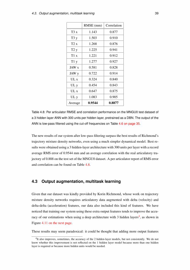
The new results of our system after low-pass filtering surpass the best results of Richmond’s

trajectory mixture density networks, even using a much simpler dynamical model. Best re-

sults were obtained using a 3 hidden-layer architecture with 300 units per layer with a record

average RMS error of 0.9544 mm and an average correlation with the real articulatory tra-

jectory of 0.888 on the test set of the MNGU0 dataset. A per articulator report of RMS error

and correlation can be found on Table 4.8.

4.3 Output augmentation, multitask learning

Given that our dataset was kindly provided by Korin Richmond, whose work on trajectory

mixture density networks requires articulatory data augmented with delta (velocity) and

delta-delta (acceleration) features, our data also included this kind of features. We have

noticed that training our system using these extra output features tends to improve the accu-

racy of our estimations when using a deep architecture with 3 hidden layers4, as shown in

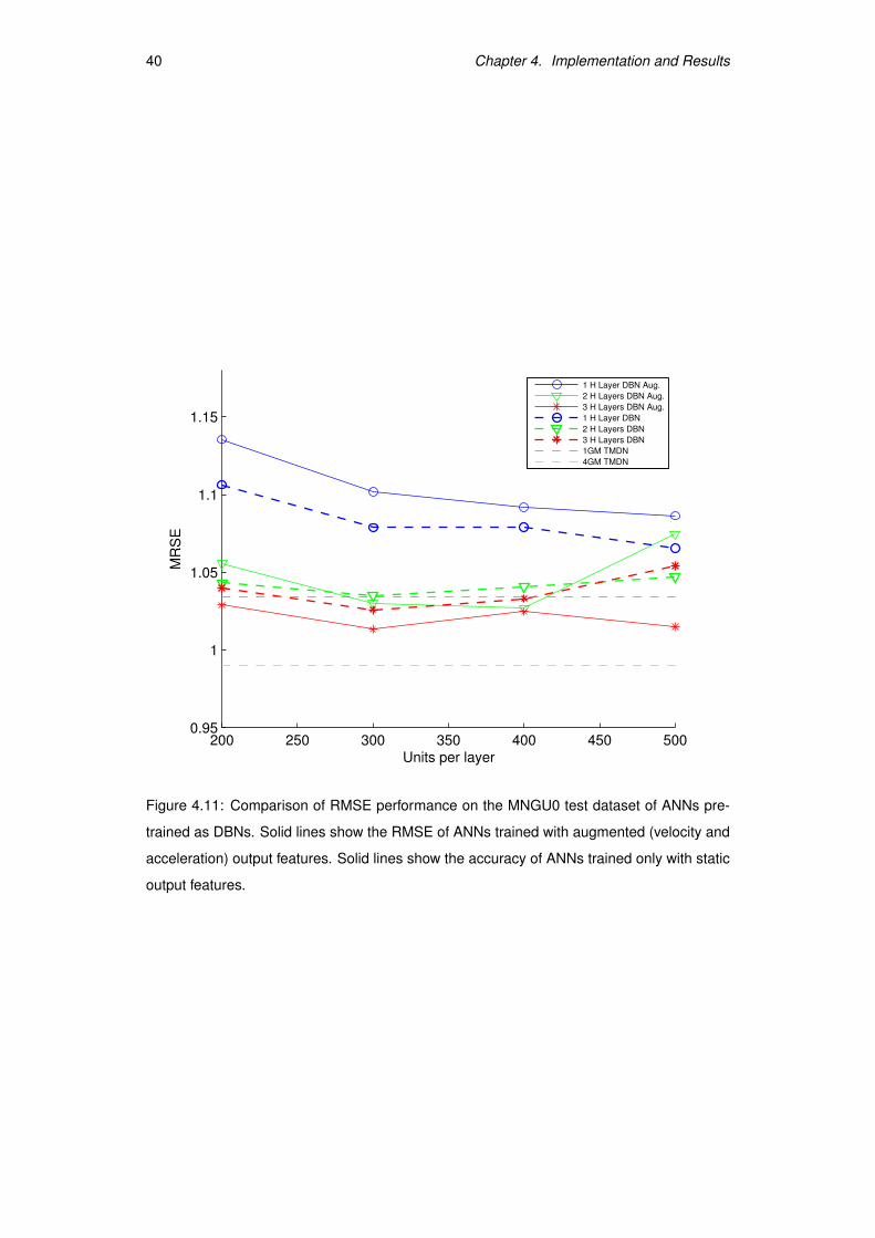
Figure 4.11 on the next page.

These results may seem paradoxical: it could be thought that adding more output features

4It also improves, sometimes, the accuracy of the 2 hidden-layer models, but not consistently. We do notknow whether this improvement is not reflected on the 1 hidden layer model because more than one hiddenlayer is required or because more hidden units would be needed.


200 250 300 350 400 450 5000.95

1

1.05

1.1

1.15

MR

SE

Units per layer

1 H Layer DBN Aug.

2 H Layers DBN Aug.

3 H Layers DBN Aug.

1 H Layer DBN

2 H Layers DBN

3 H Layers DBN

1GM TMDN

4GM TMDN

Figure 4.11: Comparison of RMSE performance on the MNGU0 test dataset of ANNs pre-

trained as DBNs. Solid lines show the RMSE of ANNs trained with augmented (velocity and

acceleration) output features. Solid lines show the accuracy of ANNs trained only with static

output features.



T3 x 1.150 0.880

T3 y 1.526 0.912

T2 x 1.268 0.881

T2 y 1.218 0.942

T1 x 1.189 0.919

T1 y 1.274 0.927

JAW x 0.580 0.829

JAW y 0.716 0.917

UL x 0.319 0.847

UL y 0.445 0.854

UL x 0.639 0.879

UL y 1.074 0.908

Average 0.9501 0.8916

Table 4.9: Per articulator RMSE and correlation performance on the MNGU0 test dataset

of a 3 hidden layer ANN with 300 units per hidden layer, pretrained as a DBN and fine-

tuned using augmented outputs. The output of the ANN is low-pass filtered using the cut-off

frequencies on Table 4.6 on page 35.

would interfere with the learning of features useful for the outputs we are really interested

in, and “compete” for the use of the internal representations. However, the beneficial effect

of augmenting the output with the right kind features has been previously recognised and

studied and is known as “multitask learning” [7].

Multitask learning argues that by trying to learn several related tasks at the same time, the

internal representation that is learned for one task can be useful in learning another task.

We ignore what kind of internal representations do dynamic (velocity and acceleration)

output features add to our network, but they appear to be useful in the light of results.

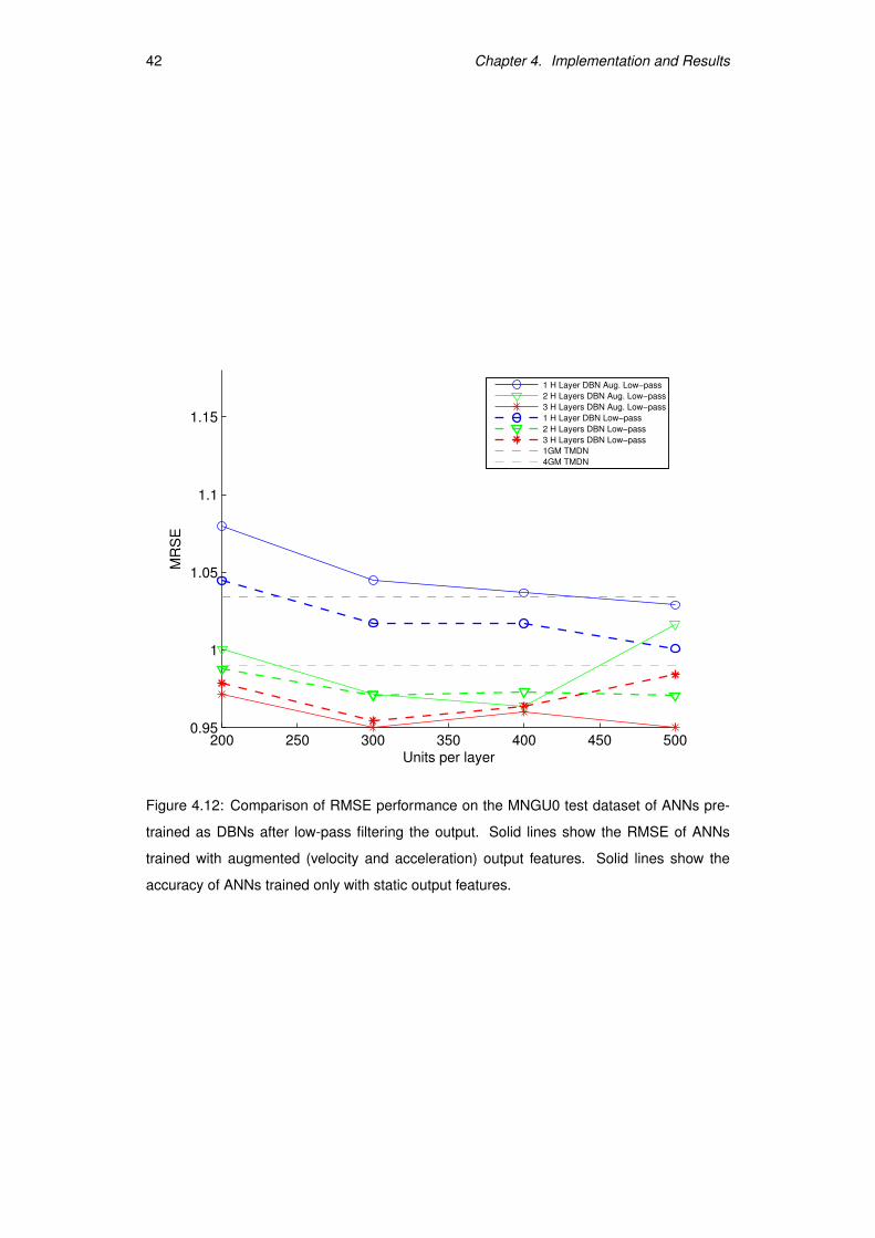
We have found a clue for the kind of representation forced by augmentation of the output,

when we low-pass filtered the output. As can be observed in Figure 4.12 on the following

page, most of the improvement acquired by doing output augmentation is lost after low-

pass filtering. This could indicate that dynamical augmentation of the output encouraged

the internal representation in the hidden layers to learn continuity features [42].

Regardless, the augmented-output 3 hidden-layer architecture with 300 units per layer achieved

slightly better results than the non-augmented version, with a record RMSE of 0.9501 mm

and a correlation with the real articulatory trajectory of 0.892 on the test set of the MNGU0

dataset. A per articulator report of RMS error and correlation can be found on Table 4.9.


200 250 300 350 400 450 5000.95

1

1.05

1.1

1.15

MR

SE

Units per layer

1 H Layer DBN Aug. Low−pass

2 H Layers DBN Aug. Low−pass

3 H Layers DBN Aug. Low−pass

1 H Layer DBN Low−pass



1GM TMDN

4GM TMDN

Figure 4.12: Comparison of RMSE performance on the MNGU0 test dataset of ANNs pre-

trained as DBNs after low-pass filtering the output. Solid lines show the RMSE of ANNs

trained with augmented (velocity and acceleration) output features. Solid lines show the

accuracy of ANNs trained only with static output features.


Unfortunately, due to the heavy computational burden of training these models, we have

not been able yet to repeat the experiments with augmented outputs a sufficient number of

times to discard the possibility of the improvement seen being just a coincidence.

Chapter 5

Conclusion

5.1 Contributions

In this work we have implemented what is, to the best of our knowledge, the first deep

architecture for articulatory inversion. We have shown that this kind of architectures are

capable of obtaining accurate estimations of the articulatory trajectories. Best results were

obtained using 3 hidden layers of 300 units each, with an RMSE of 0.95 mm on the test set

of the MNGU0 dataset. A significant error reduction compared to the previous best results

published on the same dataset of 0.99 mm using trajectory mixture density networks.

In our work, we show that adding hidden layers (up to three) to the architecture, improves

the accuracy. We also show, this is a result of a higher expressive capability of a deep

architecture [4], and not only a result of adding more parameters to the model, since a

shallow model with the same or more parameters was unable to equal the accuracy obtained

by the 3 hidden layers model.

We also show the advantage of doing unsupervised pretraining, where a deep belief network

is trained before being transformed into an artificial neural network. In all cases analysed

this had a positive effect on the results.

5.2 Limitations

There are two main limitations in our work. The first one is procedural: in order to claim

that our system is better than previous published work, we would need to repeat our exper-

iments a number of times, obtain averages of the accuracies and calculate error intervals.

However, as explained in Appendix A, training these models has a high computational cost

and no time for it was available. Nevertheless, we are confident our results will hold as

45

46 Chapter 5. Conclusion

the improvement over previous methods are quite significant in magnitude and are present

across a variety of number of hidden layers and units per layer.

The second main limitation relates to our methodology. Even though low-pass filtering im-

proves our results considerably, it would be desirable to implement a more advanced trajec-

tory method as it is done in the most recent publications by Richmond [45] or Renals [56].

Using the maximum likelihood parameter generation algorithm requires a probability dis-

tribution of the position, velocity and acceleration of the articulators. However, our present

system is only capable of inferring point estimates of those features.

5.3 Future work

In order to be able to use the maximum likelihood parameter generation algorithm, we

intend to adapt our present system to act as a “deep” mixture density network. To do this we

will have to modify our system to have as output features the mean, covariance matrix and

mixing factors of a Gaussian mixture model. These changes only affect the backpropagation

phase of the training and not the unsupervised pretraining stage. Besides, having a Gaussian

mixture as the output of our system will also allow us to explicitly tackle the non-uniqueness

of the articulatory inversion problem, leaving for the MLPG algorithm to decide the most

likely trajectory through that multimodal probability estimation.

Another research line worth exploring would include doing articulatory inversion from an

acoustic speech representation less processed than line spectral frequencies (LSF). Although

LSF appeared the best acoustic encoding for articulatory inversion in a previous comparative

study by Qin and Carreira-Perpinan [38], those studies did not include the use of deep

architectures. Given that deep architectures for phone recognition obtain better results using

simple encodings like filterbank coefficients, we hypothesise those improvements could also

be translated to the articulatory inversion domain.

Bibliography

[1] BS Atal, JJ Chang, MV Mathews, and JW Tukey. Inversion of articulatory-to-acoustic

transformation in the vocal tract by a computer-sorting technique. The Journal of the

Acoustical Society of America, 63:1535, 1978.

[2] Y. Bengio, P. Lamblin, D. Popovici, and H. Larochelle. Greedy layer-wise training of

deep networks. In Advances in Neural Information Processing Systems 19: Proceed-

ings of the 2006 Conference, volume 19, page 153. The MIT Press, 2007.

[3] Y. Bengio and Y. LeCun. Scaling learning algorithms towards AI. Large-Scale Kernel

Machines, 34, 2007.

[4] Yoshua Bengio. Learning deep architectures for AI. Foundations and Trends in Ma-

chine Learning, 2(1):1–127, 2009.

[5] C.M. Bishop. Mixture density networks. 1994.

[6] M.A. Carreira-Perpiñán and G.E. Hinton. On contrastive divergence learning.

2005:17, 2005.

[7] R. Caruana. Multitask learning. Machine Learning, 28(1):41–75, 1997.

[8] G. Casella and E.I. George. Explaining the Gibbs sampler. American Statistician,

46(3):167–174, 1992.

[9] C. Cortes and V. Vapnik. Support-vector networks. Machine learning, 20(3):273–297,

1995.

[10] G.E. Dahl, A.M. Marc Aurelio Ranzato, and G. Hinton. Phone Recognition with the

Mean-Covariance Restricted Boltzmann Machine. Advances in Neural Information

Processing Systems, 24, 2010.

[11] R.O. Duda, P.E. Hart, and D.G. Stork. Pattern classification, volume 2. Citeseer, 2001.

[12] S. Dusan and L. Deng. Estimation of articulatory parameters from speech acoustics

by kalman filtering. Proc. of CITO Researcher Retreat-Hamilton Canada, 1998.

47

48 Bibliography

[13] L.D. Erman, F. Hayes-Roth, V.R. Lesser, and D.R. Reddy. The Hearsay-II speech-

understanding system: Integrating knowledge to resolve uncertainty. ACM Computing

Surveys (CSUR), 12(2):213–253, 1980.

[14] Lee D. Erman and Victor R. Lesser. A multi-level organization for problem solving

using many, diverse, cooperating sources of knowledge. In Proceedings of the 4th

international joint conference on Artificial intelligence - Volume 1, pages 483–490,

San Francisco, CA, USA, 1975. Morgan Kaufmann Publishers Inc.

[15] G. Hinton. A practical guide to training restricted boltzmann machines. Technical

report, Department of Computer Science, University of Toronto, 2010.

[16] G.E. Hinton. Training products of experts by minimizing contrastive divergence. Neu-

ral Computation, 14(8):1771–1800, 2002.

[17] G.E. Hinton. To recognize shapes, first learn to generate images. Progress in brain

research, 165:535–547, 2007.

[18] G.E. Hinton, S. Osindero, and Y.W. Teh. A fast learning algorithm for deep belief

nets. Neural computation, 18(7):1527–1554, 2006.

[19] S. Hiroya and M. Honda. Acoustic-to-articulatory inverse mapping using an HMM-

based speech production model. In Seventh International Conference on Spoken Lan-

guage Processing, 2002.

[20] Gregor Hofer and Korin Richmond. Comparison of HMM and TMDN methods for lip

synchronisation. In Proc. Interspeech, pages 454–457, Makuhari, Japan, September

2010.

[21] K. Hornik Maxwell and H. White. Multilayer feedforward networks are universal

approximators. Neural networks, 2(5):359–366, 1989.

[22] Navdeep Jaitly and Geoffrey E. Hinton. Learning a better representation of speech

soundwaves using restricted boltzmann machines. In ICASSP, pages 5884–5887,

2011.

[23] R.E. Kalman et al. A new approach to linear filtering and prediction problems. Journal

of basic Engineering, 82(1):35–45, 1960.

[24] P. Ladefoged and K. Johnson. A course in phonetics. Wadsworth Pub Co, 2010.

[25] N. Le Roux and Y. Bengio. Representational power of restricted Boltzmann machines

and deep belief networks. Neural Computation, 20(6):1631–1649, 2008.

[26] Z. Ling, K. Richmond, J. Yamagishi, and R. Wang. Integrating articulatory features

into HMM-based parametric speech synthesis. IEEE Transactions on Audio, Speech

and Language Processing, 17(6):1171–1185, August 2009.

Bibliography 49

[27] Z.H. Ling, K. Richmond, and J. Yamagishi. An analysis of hmm-based prediction of

articulatory movements. Speech Communication, 52(10):834–846, 2010.

[28] V. Mitra, H. Nam, C.Y. Espy-Wilson, E. Saltzman, and L. Goldstein. Retrieving tract

variables from acoustics: A comparison of different machine learning strategies. Se-

lected Topics in Signal Processing, IEEE Journal of, 4(6):1027 –1045, 2010.

[29] V. Mnih. Cudamat: a cuda-based matrix class for python. Department of Computer

Science, University of Toronto, Tech. Rep. UTML TR, 4, 2009.

[30] A. Mohamed, G. Dahl, and G. Hinton. Deep Belief Networks for phone recognition. In

Proc. of NIPS 2009 Workshop on Deep Learning for Speech Recognition and Related

Applications. Citeseer, 2009.

[31] A. Mohamed, G. Dahl, and G. Hinton. Acoustic modeling using deep belief networks.

Audio, Speech, and Language Processing, IEEE Transactions on, (99), 2011.

[32] A. Mohamed, T. Sainath, G. Dahl, B. Ramabhadran, G. Hinton, and Picheny M. Deep

belief networks using discriminative features for phone recognition. In ICASSP, pages

5884–5887, 2011.

[33] A.R. Mohamed and G. Hinton. Phone recognition using restricted boltzmann ma-

chines. In Acoustics Speech and Signal Processing (ICASSP), 2010 IEEE Interna-

tional Conference on, pages 4354–4357. IEEE, 2010.

[34] N.J. Nilsson. The quest for artificial intelligence. Cambridge University Press New

York, NY, USA, 2009.

[35] G. Papcun, J. Hochberg, T.R. Thomas, F. Laroche, J. Zacks, and S. Levy. Inferring

articulation and recognizing gestures from acoustics with a neural network trained on

x-ray microbeam data. The Journal of the Acoustical Society of America, 92:688,

1992.

[36] J.S. Perkell, M.H. Cohen, M.A. Svirsky, M.L. Matthies, I. Garabieta, and M.T.T. Jack-

son. Electromagnetic midsagittal articulometer systems for transducing speech artic-

ulatory movements. The Journal of the Acoustical Society of America, 92:3078, 1992.

[37] D. Povey, D. Kanevsky, B. Kingsbury, B. Ramabhadran, G. Saon, and

K. Visweswariah. Boosted mmi for model and feature-space discriminative training.

In Acoustics, Speech and Signal Processing, 2008. ICASSP 2008. IEEE International

Conference on, pages 4057–4060. IEEE, 2008.

[38] C. Qin and M.A. Carreira-Perpiñán. A comparison of acoustic features for articulatory

inversion. In Proc. Interspeech, pages 2469–2472. Citeseer, 2007.

50 Bibliography

[39] L.R. Rabiner. A tutorial on hidden markov models and selected applications in speech

recognition. Proceedings of the IEEE, 77(2):257–286, 1989.

[40] M.G. Rahim, C.C. Goodyear, W.B. Kleijn, J. Schroeter, and M.M. Sondhi. On the

use of neural networks in articulatory speech synthesis. The Journal of the Acoustical

Society of America, 93:1109, 1993.

[41] M.A. Ranzato and G.E. Hinton. Modeling pixel means and covariances using factor-

ized third-order boltzmann machines. In Computer Vision and Pattern Recognition

(CVPR), 2010 IEEE Conference on, pages 2551–2558. IEEE, 2010.

[42] S. Renals and K. Richmond. Private communication. August 2011.

[43] K. Richmond. On exploring non-uniqueness in the inversion mapping using MDNs.

Unpublished manuscript.

[44] K. Richmond. Estimating Articulatory Parameters from the Acoustic Speech Signal.

PhD thesis, The Centre for Speech Technology Research, Edinburgh University, 2002.

[45] K. Richmond. A trajectory mixture density network for the acoustic-articulatory in-

version mapping. In Proc. Interspeech, Pittsburgh, USA, September 2006.

[46] K. Richmond. Preliminary inversion mapping results with a new EMA corpus. In

Proc. Interspeech, pages 2835–2838, Brighton, UK, September 2009.

[47] K. Richmond, P. Hoole, and King S. Announcing the electromagnetic articulography

(day 1) subset of the mngu0 articulatory corpus. In Proc. Interspeech, 2011.

[48] F. Rosenblatt. The perceptron: A probabilistic model for information storage and

organization in the brain. Psychological review, 65(6):386–408, 1958.

[49] D.E. Rumelhart, G.E. Hinton, and R.J. Williams. Learning internal representations by

error backpropagation. Parallel distributed processing, 1:318–362, 1986.

[50] R. Salakhutdinov and G. Hinton. Using deep belief nets to learn covariance kernels

for gaussian processes. Advances in neural information processing systems, 20:1249–

1256, 2008.

[51] O. Selfridge. Pandemonium: A Paradigm for Learning, Proceedings of Symposium

on the Mechanization of Thought Processes. National Physics Laboratory, 1959.

[52] H.W. Strube. Linear prediction on a warped frequency scale. The Journal of the

Acoustical Society of America, 68:1071, 1980.

[53] J. Sun and L. Deng. An overlapping-feature-based phonological model incorporating

linguistic constraints: Applications to speech recognition. The Journal of the Acousti-

cal Society of America, 111:1086, 2002.

Bibliography 51

[54] K. Tokuda, T. Yoshimura, T. Masuko, T. Kobayashi, and T. Kitamura. Speech pa-

rameter generation algorithms for HMM-based speech synthesis. pages 1315–1318,

2000.

[55] A. Wrench. Mocha-timit, 1999.

[56] L. Zhang and S. Renals. Acoustic-articulatory modeling with the trajectory HMM.

IEEE Signal Processing Letters, 15:245–248, 2008.

Appendix A

Computational setup

Comparing the performance of our GPU-based system with an initial CPU implementa-

tion we obtained a 20-fold reduction of training times when using nVidia GTX480 GPU

compared with single core of an Intel Core i7 930 CPU (5-fold when using 6 CPU cores).

However, the use of a GPU comes with some limitations, namely our system had 1.5 GB of

GPU memory which limited the number of units per layer to about 500 if we wanted to keep

the internal representations of the whole MNGU0 training dataset in the GPU’s memory. A

way to avoid this problem is to feedforward through previous layers the data just when it is

needed. Unfortunately, that solution takes away a good portion of the GPU speed-up.

Even taking advantage of GP-GPU processing, training a restricted Boltzmann machine

is a slow process. Training an RBM with 300 units in each layer takes about 30 seconds

per epoch, an RBM with 500 units per layer about 60s per epoch. Given that a typical

training experiment requires about 200 epochs, it amounts to 1.5 to 3 hours. The training

times are multiplied by the fact that an RBM has to be trained for each layer of the deep

belief network, and the many experiments required to find appropriate values for the training

configuration.

The backpropagation fine-tuning process was also implemented using GP-GPU processing.

It was found to take 1 to 3 hours depending on the number of layers and units per layer,

obtaining a 2.5 fold reduction of training times compared to using 6 CPU cores. Even

though faster algorithms could have been implemented for the fine-tuning phase, for ex-

ample scaled conjugate gradients optimization, we considered the simple backpropagation

algorithm satisfactory enough, given that most of the training time is spent, anyway, training

the restricted Boltzmann machines.

53

Documents

A Deep Belief Network for the Acoustic-Articulatory ... · A Deep Belief Network for the Acoustic-Articulatory Inversion Mapping ... The acoustic-articulatory inversion mapping problem