Inverting and Visualizing Features for Object Detection∗

Carl Vondrick, Aditya Khosla, Tomasz Malisiewicz, Antonio TorralbaMassachusetts Institute of Technology

{vondrick,khosla,tomasz,torralba}@csail.mit.edu

Abstract

This paper presents methods to visualize feature spacescommonly used in object detection. The tools in this paperallow a human to put on “feature space glasses” and seethe visual world as a computer might see it. We found thatthese “glasses” allow us to gain insight into the behaviorof computer vision systems. We show a variety of experi-ments with our visualizations, such as examining the linearseparability of recognition in HOG space, generating highscoring “super objects” for an object detector, and diag-nosing false positives. We pose the visualization problem asone of feature inversion, i.e. recovering the natural imagethat generated a feature descriptor. We describe four algo-rithms to tackle this task, with different trade-offs in speed,accuracy, and scalability. Our most successful algorithmuses ideas from sparse coding to learn a pair of dictionar-ies that enable regression between HOG features and natu-ral images, and can invert features at interactive rates. Webelieve these visualizations are useful tools to add to an ob-ject detector researcher’s toolbox, and code is available.

1. IntroductionA core building block for most modern recognition sys-

tems is a histogram of oriented gradients (HOG) [5]. Whilemachines struggle to comprehend raw pixel values, HOGprovides computers with a higher level representation of animage. The computational power of this representation hasbeen substantially demonstrated by the community in objectdetection [3, 10, 19, 24, 31] as well as scene classification[22, 29] and motion tracking [2, 11].

Yet, the human vision system processes photons—nothigh dimensional vectors—making human interpretation ofHOG features potentially counter-intuitive. As object detec-tion researchers, we often spend considerable time staring atfalse positives and asking ourselves: why does our detectorthink there is a microwave flying in the sky?

∗This paper is a pre-print of our conference paper. We have made itpublicly available early in the hopes that others find the tools described inthis paper useful. Last modified December 10, 2012.

(a) HOG (b) Inverse (This Paper) (c) Original

Figure 1: In this paper, we present several algorithms forinverting HOG descriptors back to images. The middle col-umn is generated only from HOG features.

In this paper, we attempt to give humans a microscopeinto the world of HOG. We present four algorithms for vi-sualizing and inverting HOG features back into natural im-ages. Each algorithm has different trade-offs, varying inspeed, accuracy, and scalability. Some of our algorithmsuse large databases; some are parametric. All of our algo-rithms are simple to use and understand.1

Our visualizations, shown in Fig.1, are intuitive for hu-mans to grasp while still remaining true to the informationstored inside each HOG feature, a claim we support with auser study. We found that this visualization power can giveus insight into the behavior of object detectors. For exam-

1The tools in this paper can be downloaded from http://mit.edu/vondrick/ihog.

1

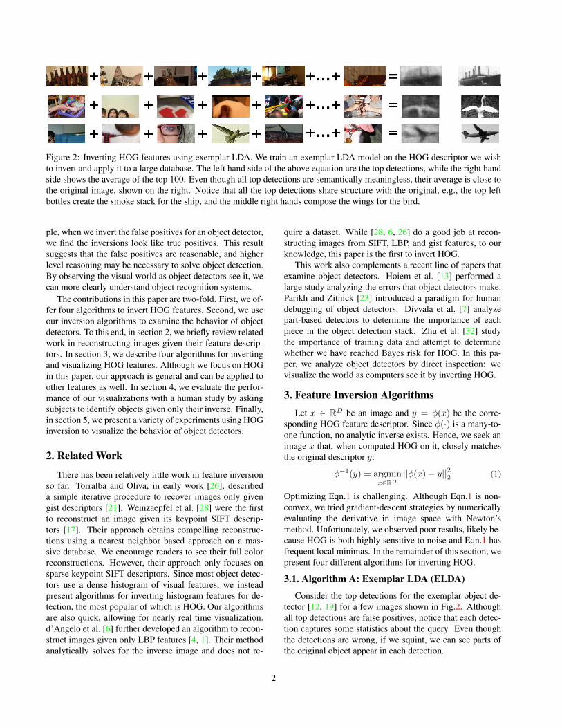
Figure 2: Inverting HOG features using exemplar LDA. We train an exemplar LDA model on the HOG descriptor we wishto invert and apply it to a large database. The left hand side of the above equation are the top detections, while the right handside shows the average of the top 100. Even though all top detections are semantically meaningless, their average is close tothe original image, shown on the right. Notice that all the top detections share structure with the original, e.g., the top leftbottles create the smoke stack for the ship, and the middle right hands compose the wings for the bird.

ple, when we invert the false positives for an object detector,we find the inversions look like true positives. This resultsuggests that the false positives are reasonable, and higherlevel reasoning may be necessary to solve object detection.By observing the visual world as object detectors see it, wecan more clearly understand object recognition systems.

The contributions in this paper are two-fold. First, we of-fer four algorithms to invert HOG features. Second, we useour inversion algorithms to examine the behavior of objectdetectors. To this end, in section 2, we briefly review relatedwork in reconstructing images given their feature descrip-tors. In section 3, we describe four algorithms for invertingand visualizing HOG features. Although we focus on HOGin this paper, our approach is general and can be applied toother features as well. In section 4, we evaluate the perfor-mance of our visualizations with a human study by askingsubjects to identify objects given only their inverse. Finally,in section 5, we present a variety of experiments using HOGinversion to visualize the behavior of object detectors.

2. Related Work

There has been relatively little work in feature inversionso far. Torralba and Oliva, in early work [26], describeda simple iterative procedure to recover images only givengist descriptors [21]. Weinzaepfel et al. [28] were the firstto reconstruct an image given its keypoint SIFT descrip-tors [17]. Their approach obtains compelling reconstruc-tions using a nearest neighbor based approach on a mas-sive database. We encourage readers to see their full colorreconstructions. However, their approach only focuses onsparse keypoint SIFT descriptors. Since most object detec-tors use a dense histogram of visual features, we insteadpresent algorithms for inverting histogram features for de-tection, the most popular of which is HOG. Our algorithmsare also quick, allowing for nearly real time visualization.d’Angelo et al. [6] further developed an algorithm to recon-struct images given only LBP features [4, 1]. Their methodanalytically solves for the inverse image and does not re-

quire a dataset. While [28, 6, 26] do a good job at recon-structing images from SIFT, LBP, and gist features, to ourknowledge, this paper is the first to invert HOG.

This work also complements a recent line of papers thatexamine object detectors. Hoiem et al. [13] performed alarge study analyzing the errors that object detectors make.Parikh and Zitnick [23] introduced a paradigm for humandebugging of object detectors. Divvala et al. [7] analyzepart-based detectors to determine the importance of eachpiece in the object detection stack. Zhu et al. [32] studythe importance of training data and attempt to determinewhether we have reached Bayes risk for HOG. In this pa-per, we analyze object detectors by direct inspection: wevisualize the world as computers see it by inverting HOG.

3. Feature Inversion AlgorithmsLet x ∈ RD be an image and y = φ(x) be the corre-

sponding HOG feature descriptor. Since φ(·) is a many-to-one function, no analytic inverse exists. Hence, we seek animage x that, when computed HOG on it, closely matchesthe original descriptor y:

φ−1(y) = argminx∈RD

||φ(x)− y||22 (1)

Optimizing Eqn.1 is challenging. Although Eqn.1 is non-convex, we tried gradient-descent strategies by numericallyevaluating the derivative in image space with Newton’smethod. Unfortunately, we observed poor results, likely be-cause HOG is both highly sensitive to noise and Eqn.1 hasfrequent local minimas. In the remainder of this section, wepresent four different algorithms for inverting HOG.

3.1. Algorithm A: Exemplar LDA (ELDA)

Consider the top detections for the exemplar object de-tector [12, 19] for a few images shown in Fig.2. Althoughall top detections are false positives, notice that each detec-tion captures some statistics about the query. Even thoughthe detections are wrong, if we squint, we can see parts ofthe original object appear in each detection.

2

We use this simple observation to produce our first inver-sion algorithm. Suppose we wish to invert HOG feature y.We first train an exemplar LDA detector [12] for this query,w = Σ−1(y − µ). We then score w against every slid-ing window on a large database. The HOG inverse is thensimply the average of the top K detections in RGB space:φ−1A (y) = 1

K

∑Ki=1 zi where zi is a top detection.

This method, although simple, produces surprisingly ac-curate reconstructions, even when the database does notcontain the category of the HOG template. We note thatthis method may be subject to dataset bias [25] but couldbe overcome [15]. We also point out that a similar nearestneighbor method is used in brain research to visualize whata person might be seeing [20].

3.2. Algorithm B: Ridge Regression

Unfortunately, running an object detector across a largedatabase is computationally expensive. In this section, wepresent a fast, parametric inversion algorithm.

Let X ∈ RD be a random variable representing a grayscale image and Y ∈ Rd be a random variable of its corre-sponding HOG point. We define these random variablesto be normally distributed on a D + d-variate GaussianP (X,Y ) ∼ N (µ,Σ) with parameters µ = [ µX µY ] andΣ =

[ΣXX ΣXY

ΣTXY ΣY Y

]. In order to invert a HOG feature y, we

calculate the most likely image from the Gaussian P condi-tioned on Y = y:

φ−1B (y) = argmax

x∈RD

P (X = x|Y = y) (2)

It is well known that Gaussians have a closed form condi-tional mode:

φ−1B (y) = ΣXY Σ−1

Y Y (y − µY ) + µX (3)

Under this inversion algorithm, any HOG point can be in-verted by a single matrix multiplication, allowing for inver-sion in under a second.

We estimate µ and Σ on a large database. In practice, Σis not positive definite; we add a small uniform prior (i.e.,Σ = Σ + λI) so Σ can be inverted. Since we wish to invertany HOG point, we assume that P (X,Y ) is stationary [12],allowing us to efficiently learn the covariance across mas-sive datasets. We invert a arbitrary dimensional HOG pointby marginalizing out unused dimensions.

3.3. Algorithm C: Direct Optimization

We found that ridge regression yields blurred inversions.Intuitively, since HOG is invariant to shifts up to its bin size,there are many images that map to the same HOG point.Ridge regression is reporting the statistically most likelyimage, which is the average over all shifts. This causesridge regression to only recover the low frequencies of theoriginal image.

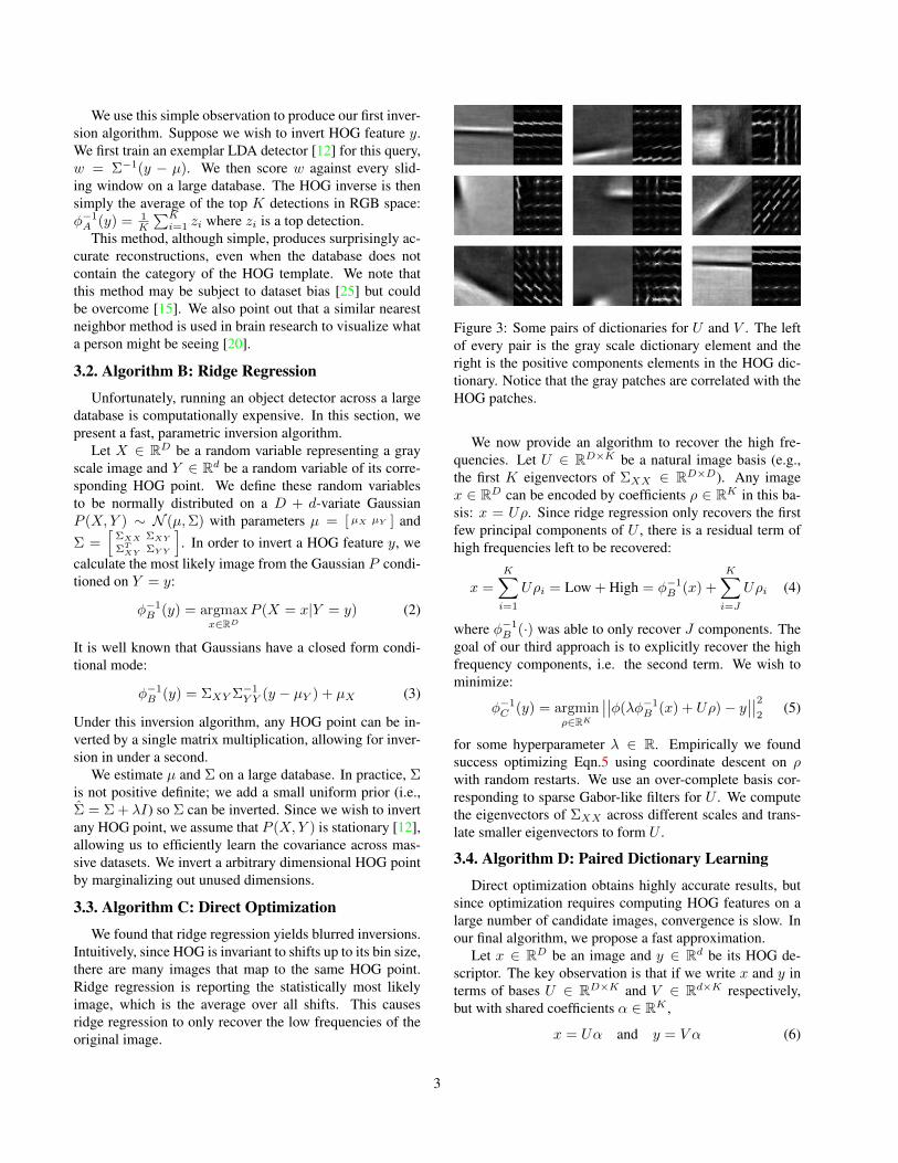
Figure 3: Some pairs of dictionaries for U and V . The leftof every pair is the gray scale dictionary element and theright is the positive components elements in the HOG dic-tionary. Notice that the gray patches are correlated with theHOG patches.

We now provide an algorithm to recover the high fre-quencies. Let U ∈ RD×K be a natural image basis (e.g.,the first K eigenvectors of ΣXX ∈ RD×D). Any imagex ∈ RD can be encoded by coefficients ρ ∈ RK in this ba-sis: x = Uρ. Since ridge regression only recovers the firstfew principal components of U , there is a residual term ofhigh frequencies left to be recovered:

x =

K∑i=1

Uρi = Low + High = φ−1B (x) +

K∑i=J

Uρi (4)

where φ−1B (·) was able to only recover J components. The

goal of our third approach is to explicitly recover the highfrequency components, i.e. the second term. We wish tominimize:

φ−1C (y) = argmin

ρ∈RK

∣∣∣∣φ(λφ−1B (x) + Uρ)− y

∣∣∣∣22

(5)

for some hyperparameter λ ∈ R. Empirically we foundsuccess optimizing Eqn.5 using coordinate descent on ρwith random restarts. We use an over-complete basis cor-responding to sparse Gabor-like filters for U . We computethe eigenvectors of ΣXX across different scales and trans-late smaller eigenvectors to form U .

3.4. Algorithm D: Paired Dictionary Learning

Direct optimization obtains highly accurate results, butsince optimization requires computing HOG features on alarge number of candidate images, convergence is slow. Inour final algorithm, we propose a fast approximation.

Let x ∈ RD be an image and y ∈ Rd be its HOG de-scriptor. The key observation is that if we write x and y interms of bases U ∈ RD×K and V ∈ Rd×K respectively,but with shared coefficients α ∈ RK ,

x = Uα and y = V α (6)

3

then inversion can be obtained by first projecting the HOGfeatures y onto the HOG basis V , then projecting α into thenatural image basis U :

φ−1D (y) = Uα (7)

where α = argminα||y − V α|| s.t. ||α||1 ≤ λ (8)

Since efficient solvers for Eqn.8 exist [18, 16], we are ableto invert HOG patches in under a second.

This paired dictionary trick requires finding appropriatebases U and V such that Eqn.6 holds. To do this, we solvea paired dictionary learning problem, inspired by recent su-perresolution sparse coding work [30, 27]:

argminU,V,α

N∑i=1

(||xi − Uαi||22 + ||φ(xi)− V αi||22

)s.t. ||αi||1 ≤ λ ∀i, ||U ||22 ≤ γ1, ||V ||22 ≤ γ2

(9)

After a few algebraic manipulations, the above objectivesimplifies to a standard sparse coding and dictionary learn-ing problem with concatenated dictionaries, which we opti-mize using SPAMS [18]. Optimization typically took a fewhours on medium sized problems. We estimate U and Vwith a dictionary size K ∈ O(103) and training samplesN ∈ O(106) from a large database. See Fig.3 for a visual-ization of the learned dictionary pairs.

Unfortunately, the paired dictionary learning formula-tion suffers on problems of nontrivial scale. In practice, weonly learn dictionaries for 5 × 5 HOG templates. In orderto invert a w × h HOG template y, we invert every 5 × 5subpatch inside y and average overlapping patches in the fi-nal reconstruction. We found that this approximation workswell in practice.

4. EvaluationIn this section, we evaluate our four inversion algorithms

using both qualitative and quantitative measures. We usePASCAL VOC 2011 [8] as our dataset and we invert patchescorresponding to objects. Any algorithm that required train-ing could only access the training set. During evaluation,only images from the validation set are examined. Thedatabase for exemplar LDA excluded the category of thepatch we were inverting to reduce the effect of biases.

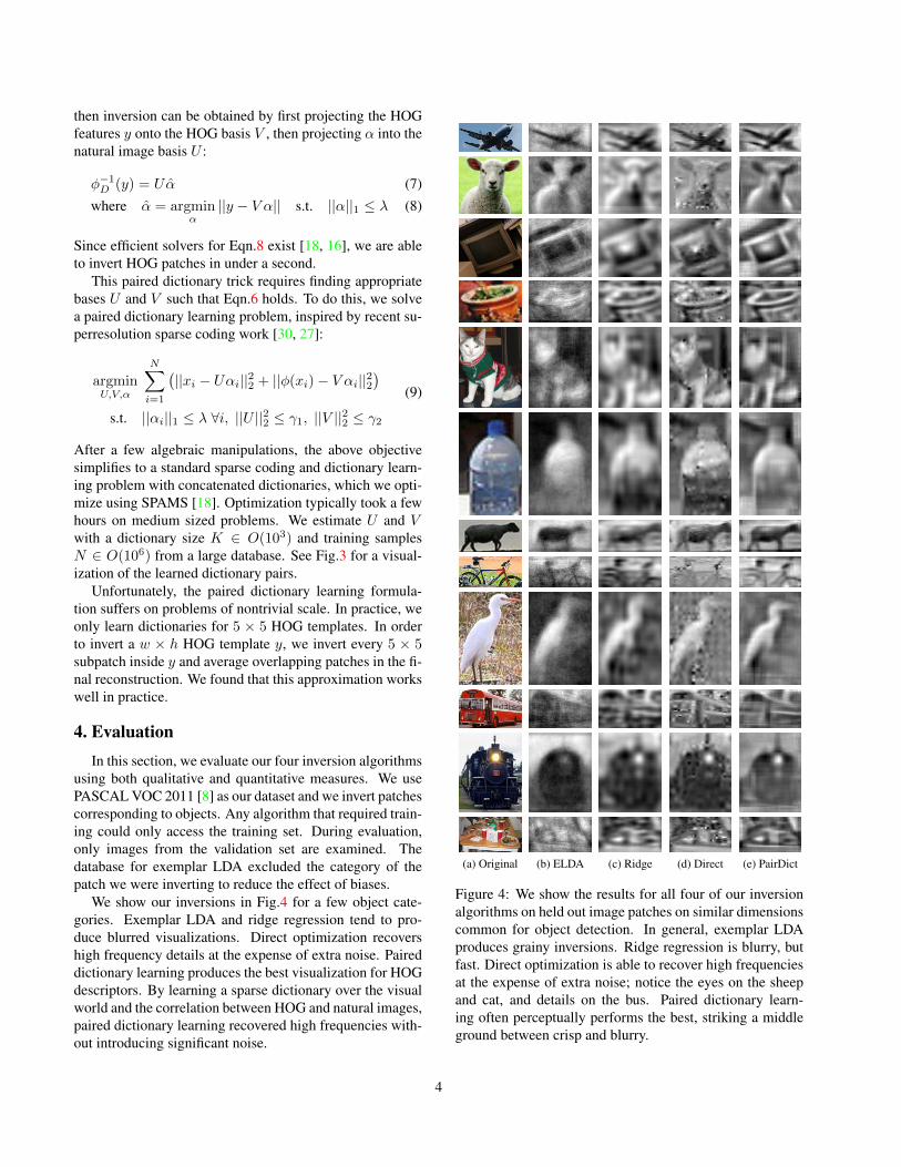
We show our inversions in Fig.4 for a few object cate-gories. Exemplar LDA and ridge regression tend to pro-duce blurred visualizations. Direct optimization recovershigh frequency details at the expense of extra noise. Paireddictionary learning produces the best visualization for HOGdescriptors. By learning a sparse dictionary over the visualworld and the correlation between HOG and natural images,paired dictionary learning recovered high frequencies with-out introducing significant noise.

(a) Original (b) ELDA (c) Ridge (d) Direct (e) PairDict

Figure 4: We show the results for all four of our inversionalgorithms on held out image patches on similar dimensionscommon for object detection. In general, exemplar LDAproduces grainy inversions. Ridge regression is blurry, butfast. Direct optimization is able to recover high frequenciesat the expense of extra noise; notice the eyes on the sheepand cat, and details on the bus. Paired dictionary learn-ing often perceptually performs the best, striking a middleground between crisp and blurry.

4

Category ELDA Ridge Direct PairDictaeroplane 0.634 0.633 0.596 0.609bicycle 0.452 0.577 0.513 0.561bus 0.627 0.632 0.587 0.585cat 0.749 0.712 0.687 0.705cow 0.720 0.663 0.632 0.650horse 0.686 0.633 0.586 0.635tvmonitor 0.711 0.640 0.638 0.629Mean 0.671 0.656 0.620 0.637

Table 1: We evaluate the performance of our inversion al-gorithm by comparing the inverse to the ground truth imageusing the mean normalized cross correlation. Higher is bet-ter; a score of 1 is perfect. In general, exemplar LDA doesslightly better at reconstructing the original pixels.

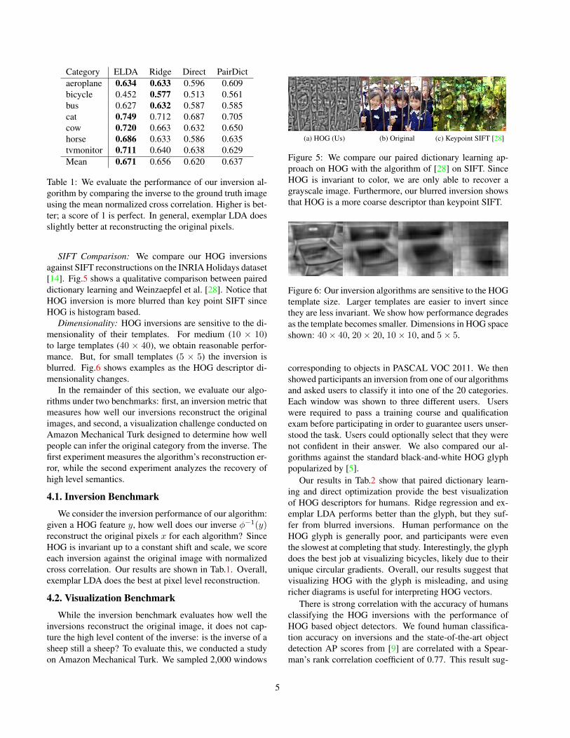
SIFT Comparison: We compare our HOG inversionsagainst SIFT reconstructions on the INRIA Holidays dataset[14]. Fig.5 shows a qualitative comparison between paireddictionary learning and Weinzaepfel et al. [28]. Notice thatHOG inversion is more blurred than key point SIFT sinceHOG is histogram based.

Dimensionality: HOG inversions are sensitive to the di-mensionality of their templates. For medium (10 × 10)to large templates (40 × 40), we obtain reasonable perfor-mance. But, for small templates (5 × 5) the inversion isblurred. Fig.6 shows examples as the HOG descriptor di-mensionality changes.

In the remainder of this section, we evaluate our algo-rithms under two benchmarks: first, an inversion metric thatmeasures how well our inversions reconstruct the originalimages, and second, a visualization challenge conducted onAmazon Mechanical Turk designed to determine how wellpeople can infer the original category from the inverse. Thefirst experiment measures the algorithm’s reconstruction er-ror, while the second experiment analyzes the recovery ofhigh level semantics.

4.1. Inversion Benchmark

We consider the inversion performance of our algorithm:given a HOG feature y, how well does our inverse φ−1(y)reconstruct the original pixels x for each algorithm? SinceHOG is invariant up to a constant shift and scale, we scoreeach inversion against the original image with normalizedcross correlation. Our results are shown in Tab.1. Overall,exemplar LDA does the best at pixel level reconstruction.

4.2. Visualization Benchmark

While the inversion benchmark evaluates how well theinversions reconstruct the original image, it does not cap-ture the high level content of the inverse: is the inverse of asheep still a sheep? To evaluate this, we conducted a studyon Amazon Mechanical Turk. We sampled 2,000 windows

(a) HOG (Us) (b) Original (c) Keypoint SIFT [28]

Figure 5: We compare our paired dictionary learning ap-proach on HOG with the algorithm of [28] on SIFT. SinceHOG is invariant to color, we are only able to recover agrayscale image. Furthermore, our blurred inversion showsthat HOG is a more coarse descriptor than keypoint SIFT.

Figure 6: Our inversion algorithms are sensitive to the HOGtemplate size. Larger templates are easier to invert sincethey are less invariant. We show how performance degradesas the template becomes smaller. Dimensions in HOG spaceshown: 40× 40, 20× 20, 10× 10, and 5× 5.

corresponding to objects in PASCAL VOC 2011. We thenshowed participants an inversion from one of our algorithmsand asked users to classify it into one of the 20 categories.Each window was shown to three different users. Userswere required to pass a training course and qualificationexam before participating in order to guarantee users unser-stood the task. Users could optionally select that they werenot confident in their answer. We also compared our al-gorithms against the standard black-and-white HOG glyphpopularized by [5].

Our results in Tab.2 show that paired dictionary learn-ing and direct optimization provide the best visualizationof HOG descriptors for humans. Ridge regression and ex-emplar LDA performs better than the glyph, but they suf-fer from blurred inversions. Human performance on theHOG glyph is generally poor, and participants were eventhe slowest at completing that study. Interestingly, the glyphdoes the best job at visualizing bicycles, likely due to theirunique circular gradients. Overall, our results suggest thatvisualizing HOG with the glyph is misleading, and usingricher diagrams is useful for interpreting HOG vectors.

There is strong correlation with the accuracy of humansclassifying the HOG inversions with the performance ofHOG based object detectors. We found human classifica-tion accuracy on inversions and the state-of-the-art objectdetection AP scores from [9] are correlated with a Spear-man’s rank correlation coefficient of 0.77. This result sug-

5

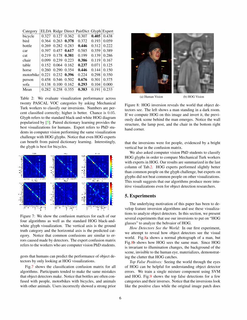
Category ELDA Ridge Direct PairDict Glyph Expertbicycle 0.327 0.127 0.362 0.307 0.405 0.438bird 0.364 0.263 0.378 0.372 0.193 0.059bottle 0.269 0.282 0.283 0.446 0.312 0.222car 0.397 0.457 0.617 0.585 0.359 0.389cat 0.219 0.178 0.381 0.199 0.139 0.286chair 0.099 0.239 0.223 0.386 0.119 0.167table 0.152 0.064 0.162 0.237 0.071 0.125horse 0.260 0.290 0.354 0.446 0.144 0.150motorbike 0.221 0.232 0.396 0.224 0.298 0.350person 0.458 0.546 0.502 0.676 0.301 0.375sofa 0.138 0.100 0.162 0.293 0.104 0.000Mean 0.282 0.258 0.355 0.383 0.191 0.233

Table 2: We evaluate visualization performance acrosstwenty PASCAL VOC categories by asking MechanicalTurk workers to classify our inversions. Numbers are per-cent classified correctly; higher is better. Chance is 0.05.Glyph refers to the standard black-and-white HOG diagrampopularized by [5]. Paired dictionary learning provides thebest visualizations for humans. Expert refers to PhD stu-dents in computer vision performing the same visualizationchallenge with HOG glyphs. Notice that even HOG expertscan benefit from paired dictionary learning. Interestingly,the glyph is best for bicycles.

Figure 7: We show the confusion matrices for each of ourfour algorithms as well as the standard HOG black-and-white glyph visualization. The vertical axis is the groundtruth category and the horizontal axis is the predicted cat-egory. Notice that common confusions are similar to er-rors caused made by detectors. The expert confusion matrixrefers to the workers who are computer vision PhD students.

gests that humans can predict the performance of object de-tectors by only looking at HOG visualizations.

Fig.7 shows the classification confusion matrix for allalgorithms. Participants tended to make the same mistakesthat object detectors make. Notice that bottles are often con-fused with people, motorbikes with bicycles, and animalswith other animals. Users incorrectly showed a strong prior

(a) Human Vision (b) HOG Vision

Figure 8: HOG inversion reveals the world that object de-tectors see. The left shows a man standing in a dark room.If we compute HOG on this image and invert it, the previ-ously dark scene behind the man emerges. Notice the wallstructure, the lamp post, and the chair in the bottom righthand corner.

that the inversions were for people, evidenced by a brightvertical bar in the confusion matrix.

We also asked computer vision PhD students to classifyHOG glyphs in order to compare Mechanical Turk workerswith experts in HOG. Our results are summarized in the lastcolumn of Tab.2. HOG experts performed slightly betterthan common people on the glyph challenge, but experts onglyphs did not beat common people on other visualizations.This result suggests that our algorithms produce more intu-itive visualizations even for object detection researchers.

5. ExperimentsThe underlying motivation of this paper has been to de-

velop feature inversion algorithms and use these visualiza-tions to analyze object detectors. In this section, we presentseveral experiments that use our inversions to put on “HOGglasses” to analyze the behvaior of HOG.

How Detectors See the World: In our first experiment,we attempt to reveal how object detectors see the visualworld. Fig.8a shows a normal photograph of a man, butFig.8b shows how HOG sees the same man. Since HOGis invariant to illumination changes, the background of thescene, invisible to the human eye, materializes, demonstrat-ing the clutter that HOG catches.

Top False Positives: Seeing the world through the eyesof HOG can be helpful for understanding object detectorerrors. We train a single mixture component using SVMand HOG. Fig.9 shows the top false detections for a fewcategories and their inverses. Notice that the inversions looklike the positive class while the original image patch does

6

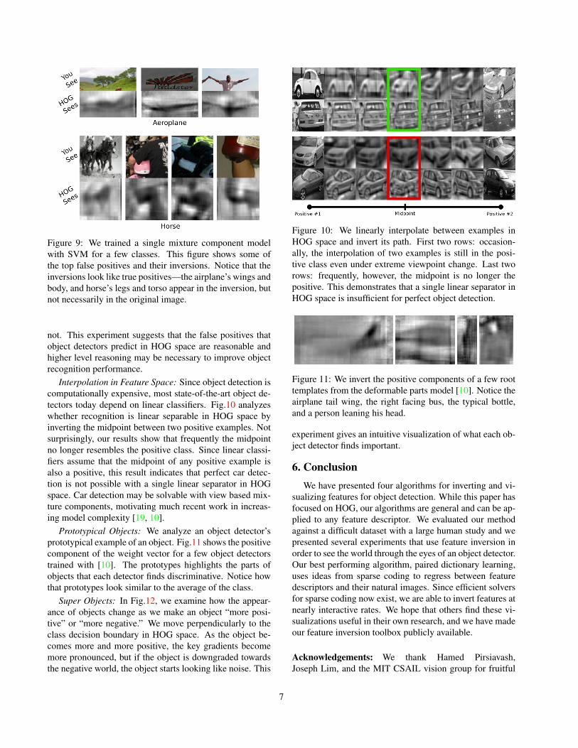
Figure 9: We trained a single mixture component modelwith SVM for a few classes. This figure shows some ofthe top false positives and their inversions. Notice that theinversions look like true positives—the airplane’s wings andbody, and horse’s legs and torso appear in the inversion, butnot necessarily in the original image.

not. This experiment suggests that the false positives thatobject detectors predict in HOG space are reasonable andhigher level reasoning may be necessary to improve objectrecognition performance.

Interpolation in Feature Space: Since object detection iscomputationally expensive, most state-of-the-art object de-tectors today depend on linear classifiers. Fig.10 analyzeswhether recognition is linear separable in HOG space byinverting the midpoint between two positive examples. Notsurprisingly, our results show that frequently the midpointno longer resembles the positive class. Since linear classi-fiers assume that the midpoint of any positive example isalso a positive, this result indicates that perfect car detec-tion is not possible with a single linear separator in HOGspace. Car detection may be solvable with view based mix-ture components, motivating much recent work in increas-ing model complexity [19, 10].

Prototypical Objects: We analyze an object detector’sprototypical example of an object. Fig.11 shows the positivecomponent of the weight vector for a few object detectorstrained with [10]. The prototypes highlights the parts ofobjects that each detector finds discriminative. Notice howthat prototypes look similar to the average of the class.

Super Objects: In Fig.12, we examine how the appear-ance of objects change as we make an object “more posi-tive” or “more negative.” We move perpendicularly to theclass decision boundary in HOG space. As the object be-comes more and more positive, the key gradients becomemore pronounced, but if the object is downgraded towardsthe negative world, the object starts looking like noise. This

Figure 10: We linearly interpolate between examples inHOG space and invert its path. First two rows: occasion-ally, the interpolation of two examples is still in the posi-tive class even under extreme viewpoint change. Last tworows: frequently, however, the midpoint is no longer thepositive. This demonstrates that a single linear separator inHOG space is insufficient for perfect object detection.

Figure 11: We invert the positive components of a few roottemplates from the deformable parts model [10]. Notice theairplane tail wing, the right facing bus, the typical bottle,and a person leaning his head.

experiment gives an intuitive visualization of what each ob-ject detector finds important.

6. ConclusionWe have presented four algorithms for inverting and vi-

sualizing features for object detection. While this paper hasfocused on HOG, our algorithms are general and can be ap-plied to any feature descriptor. We evaluated our methodagainst a difficult dataset with a large human study and wepresented several experiments that use feature inversion inorder to see the world through the eyes of an object detector.Our best performing algorithm, paired dictionary learning,uses ideas from sparse coding to regress between featuredescriptors and their natural images. Since efficient solversfor sparse coding now exist, we are able to invert features atnearly interactive rates. We hope that others find these vi-sualizations useful in their own research, and we have madeour feature inversion toolbox publicly available.

Acknowledgements: We thank Hamed Pirsiavash,Joseph Lim, and the MIT CSAIL vision group for fruitful

7

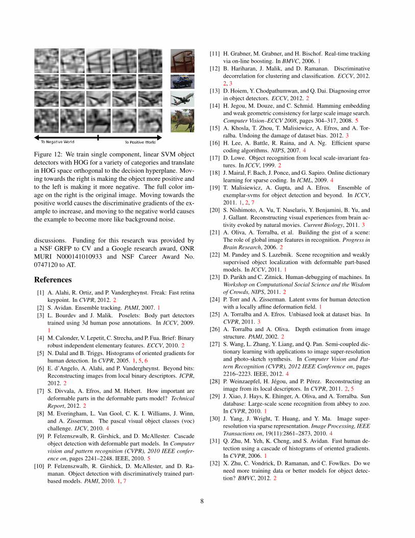
Figure 12: We train single component, linear SVM objectdetectors with HOG for a variety of categories and translatein HOG space orthogonal to the decision hyperplane. Mov-ing towards the right is making the object more positive andto the left is making it more negative. The full color im-age on the right is the original image. Moving towards thepositive world causes the discriminative gradients of the ex-ample to increase, and moving to the negative world causesthe example to become more like background noise.

discussions. Funding for this research was provided bya NSF GRFP to CV and a Google research award, ONRMURI N000141010933 and NSF Career Award No.0747120 to AT.

References[1] A. Alahi, R. Ortiz, and P. Vandergheynst. Freak: Fast retina

keypoint. In CVPR, 2012. 2[2] S. Avidan. Ensemble tracking. PAMI, 2007. 1[3] L. Bourdev and J. Malik. Poselets: Body part detectors

trained using 3d human pose annotations. In ICCV, 2009.1

[4] M. Calonder, V. Lepetit, C. Strecha, and P. Fua. Brief: Binaryrobust independent elementary features. ECCV, 2010. 2

[5] N. Dalal and B. Triggs. Histograms of oriented gradients forhuman detection. In CVPR, 2005. 1, 5, 6

[6] E. d’Angelo, A. Alahi, and P. Vandergheynst. Beyond bits:Reconstructing images from local binary descriptors. ICPR,2012. 2

[7] S. Divvala, A. Efros, and M. Hebert. How important aredeformable parts in the deformable parts model? TechnicalReport, 2012. 2

[8] M. Everingham, L. Van Gool, C. K. I. Williams, J. Winn,and A. Zisserman. The pascal visual object classes (voc)challenge. IJCV, 2010. 4

[9] P. Felzenszwalb, R. Girshick, and D. McAllester. Cascadeobject detection with deformable part models. In Computervision and pattern recognition (CVPR), 2010 IEEE confer-ence on, pages 2241–2248. IEEE, 2010. 5

[10] P. Felzenszwalb, R. Girshick, D. McAllester, and D. Ra-manan. Object detection with discriminatively trained part-based models. PAMI, 2010. 1, 7

[11] H. Grabner, M. Grabner, and H. Bischof. Real-time trackingvia on-line boosting. In BMVC, 2006. 1

[12] B. Hariharan, J. Malik, and D. Ramanan. Discriminativedecorrelation for clustering and classification. ECCV, 2012.2, 3

[13] D. Hoiem, Y. Chodpathumwan, and Q. Dai. Diagnosing errorin object detectors. ECCV, 2012. 2

[14] H. Jegou, M. Douze, and C. Schmid. Hamming embeddingand weak geometric consistency for large scale image search.Computer Vision–ECCV 2008, pages 304–317, 2008. 5

[15] A. Khosla, T. Zhou, T. Malisiewicz, A. Efros, and A. Tor-ralba. Undoing the damage of dataset bias. 2012. 3

[16] H. Lee, A. Battle, R. Raina, and A. Ng. Efficient sparsecoding algorithms. NIPS, 2007. 4

[17] D. Lowe. Object recognition from local scale-invariant fea-tures. In ICCV, 1999. 2

[18] J. Mairal, F. Bach, J. Ponce, and G. Sapiro. Online dictionarylearning for sparse coding. In ICML, 2009. 4

[19] T. Malisiewicz, A. Gupta, and A. Efros. Ensemble ofexemplar-svms for object detection and beyond. In ICCV,2011. 1, 2, 7

[20] S. Nishimoto, A. Vu, T. Naselaris, Y. Benjamini, B. Yu, andJ. Gallant. Reconstructing visual experiences from brain ac-tivity evoked by natural movies. Current Biology, 2011. 3

[21] A. Oliva, A. Torralba, et al. Building the gist of a scene:The role of global image features in recognition. Progress inBrain Research, 2006. 2

[22] M. Pandey and S. Lazebnik. Scene recognition and weaklysupervised object localization with deformable part-basedmodels. In ICCV, 2011. 1

[23] D. Parikh and C. Zitnick. Human-debugging of machines. InWorkshop on Computational Social Science and the Wisdomof Crowds, NIPS, 2011. 2

[24] P. Torr and A. Zisserman. Latent svms for human detectionwith a locally affine deformation field. 1

[25] A. Torralba and A. Efros. Unbiased look at dataset bias. InCVPR, 2011. 3

[26] A. Torralba and A. Oliva. Depth estimation from imagestructure. PAMI, 2002. 2

[27] S. Wang, L. Zhang, Y. Liang, and Q. Pan. Semi-coupled dic-tionary learning with applications to image super-resolutionand photo-sketch synthesis. In Computer Vision and Pat-tern Recognition (CVPR), 2012 IEEE Conference on, pages2216–2223. IEEE, 2012. 4

[28] P. Weinzaepfel, H. Jegou, and P. Perez. Reconstructing animage from its local descriptors. In CVPR, 2011. 2, 5

[29] J. Xiao, J. Hays, K. Ehinger, A. Oliva, and A. Torralba. Sundatabase: Large-scale scene recognition from abbey to zoo.In CVPR, 2010. 1

[30] J. Yang, J. Wright, T. Huang, and Y. Ma. Image super-resolution via sparse representation. Image Processing, IEEETransactions on, 19(11):2861–2873, 2010. 4

[31] Q. Zhu, M. Yeh, K. Cheng, and S. Avidan. Fast human de-tection using a cascade of histograms of oriented gradients.In CVPR, 2006. 1

[32] X. Zhu, C. Vondrick, D. Ramanan, and C. Fowlkes. Do weneed more training data or better models for object detec-tion? BMVC, 2012. 2

8