Inverse Problems: Recovery of BV Coefficients

from Nodes

by

Ole H. Hald

University of California, Berkeley

Berkeley, California 94720

and

Joyce R. McLaughlin

Rensselaer Polytechnic Institute

Troy, New York 12181

1

Abstract

Consider the Sturm-Liouville problem on a finite interval with Dirichlet bound-

ary conditions. Let the elastic modulus and the density be of bounded variation.

Results for both the forward problem and the inverse problem are established.

For the forward problem, new bounds are established for the eigenfrequencies.

The bounds are sharp. For the inverse problem, it is shown that the elastic

modulus is uniquely determined, up to one arbitrary constant, by a dense sub-

set of the nodes of the eigenfunctions when the density is known. Similarly

it is shown that the density is uniquely determined, up to one arbitrary con-

stant, by a dense subset of the nodes of the eigenfunctions when the elastic

modulus is known. Algorithms for finding piecewise constant approximates to

the unknown elastic modulus or density are established and shown to converge

to the unknown function at every point of continuity. Results from numerical

calculations are exhibited.

Running head: Recovery of BV Coefficients

Subject Classification: 34B24, 34L15, 73D50

2

Section 1: Introduction

Consider the longitudinal vibrations of a rod. Consider the transverse vibrations of a

string. Suppose that the density and/or the elastic modulus are variable and possess sharp

discontinuities. We then ask two questions. The first is: Can an accurate estimate be

made of the natural frequencies? Our answer is to give new bounds for the frequencies.

The second question is: Can the density and/or the elastic modulus be determined from the

nodal positions? We prove uniqueness results, present algorithms for finding the density

or stiffness, and exhibit the results of numerical experiments.

The squares of the natural frequencies are the eigenvalues for a Sturm-Liouville bound-

ary value problem. The asymptotic forms for these eigenvalues has a long history. If the

density and the elastic modulus have integrable second derivatives the asymptotic forms

are well known, see e.g. [B], [GL], [Ho], [L], [M], [PT], and more recently [C2] when the

ends of the beam are fixed and [B], [GL], [IT], [Ho], [L], [M], [HMcL] when mixed bound-

ary conditions are satisfied. In each case the nth eigenvalue is equal to a constant times

(nπ)2 plus a term of order one. If the density and elastic modulus are not that smooth,

then results are more recent. For the case where these coefficients have integrable first

derivatives, see [HMcL], [CMcL], [A1], [A2]. There it is shown that the square root of the

eigenvalue is a constant times nπ plus a small o(1) term. If the coefficients have square

integrable first derivatives, then the sequence of o(1) terms is in `2. Finally, if the coef-

ficients have a finite number of discontinuities and have continuous or square integrable

second derivatives between the discontinuities, results on the distribution of eigenvalues

can be found in [MAL],[H], [Wi], or [C1]. For coefficients of bounded variation see also

[A2] where an asymptotic form is not exhibited but it is shown that the eigenvalues are

roots of a function with specified properties. The new feature when the elastic modulus

and density can have discontinuities is that the square root of the eigenvalue does not, in

general, approach a constant multiple of nπ.

Here we assume that the stiffness and density are of bounded variation and hence

can have a countable number of discontinuities. We exhibit four separate bounds for the

3

difference between a constant times the square root of the eigenvalue and nπ. The first

bound applies when the density and stiffness coefficients are of bounded variation. We

show that this bound is sharp for continuous functions of bounded variation. The second

bound is for piecewise constant functions with a finite number of discontinuities. We

demonstrate that this bound is sharp. The third bound is a combination of the first two.

It applies when the stiffness and density are of bounded variation and have a finite number

of discontinuities. The final bound applies when the stiffness and density have an infinite

number of discontinuities. Numerical calculations are presented to support our results.

This is done in Section 2.

The remaining sections of this paper address the inverse nodal problem. One-dimensional

inverse nodal problems have previously been considered in [McL], [HMcL1], [HMcL2], [S],

[ST]. There it is shown that under sufficient smoothness assumptions for the coefficients,

a single coefficient is uniquely determined up to one arbitrary constant by a dense subset

of nodes. See also [BS] for uniqueness results when the boundary conditions contain the

eigenvalue parameter. Further, it is announced in [HMcL1] that two sufficiently smooth

coefficients can both be uniquely determined, up to two arbitrary constants, by a dense

subset of the nodes. Here we establish uniqueness results for two cases where the coef-

ficients are not so smooth. In each case either the elastic modulus or the density, but

not both, is of bounded variation. The other coefficient is constant. It could also be a

known function of bounded variation. It is shown that the unknown variable coefficient

is uniquely determined, up to one arbitrary constant, at every point of continuity by a

dense subset of adjacent pairs of nodal positions. This is done in Section 3. In Section

4, simple algorithms for computing piecewise constant approximations for the unknown

variable coefficients are presented. Prior algorithms are contained in [HMcL1], [HMcL2],

[S] and [ST] under sufficient smoothness assumptions. Here it is shown that the piecewise

constant approximations converge to the desired (bounded variation) coefficients at each

point of continuity. The data that is used for each piecewise constant approximation is one

natural frequency and all the nodal positions for the corresponding mode shape. This data

can be obtained by performing the following experiment: Excite a rod longitudinally at a

natural frequency. Measure that frequency. Then scan the rod with a lazer. At each point,

4

measure the Doppler shift in the backscatter. The places on the rod where the Doppler

shift is minimized are the nodes. There is a similar experiment for obtaining the data for

a vibrating string.

In the remaining section, Section 5, numerical computations that illustrate the accuracy

of the algorithms are presented. Other examples to show how well the piecewise constant

approximations estimate the variable coefficient when the coefficient is of bounded variation

were previously presented in [HMcL3].

5

Section 2: Bounds for the Eigenvalues

Consider the longitudinal vibration of a rod. The rod has fixed ends and both the elasticity

coefficient, p, and density, ρ, are variable. Let m be a positive constant and require that

0 < m < p, ρ. Let p, ρ ∈ BV [0, L], continuous from the right and at x = L. Then we

obtain the natural frequencies, ωn/2π, and the corresponding mode shapes, yn, from the

eigenvalues, ω2n, and the corresponding eigenfunctions, yn, n = 1, 2, ..., for

(pyx)x + ω2ρy = 0, 0 ≤ x ≤ L, (1)

y(0) = y(L) = 0. (2)

The goal of this section is to establish new bounds for the nth eigenfrequency ωn. We

state six theorems. Four theorems give the bounds and two additional theorems establish

that the bounds are sharp. We also establish a crude bound for the distance between

consecutive nodes or zeros of yn.

We say that y is a solution of (1) if y is absolutely continuous, pyx is absolutely continu-

ous and the differential equation is satisfied a.e.. It is known, see [At], that this eigenvalue

problem has a sequence of eigenvalues 0 < ω21 < ω2

2 < . . . with limn→∞ ω2n = ∞. For

each eigenvalue, ω2n, the corresponding eigenfunction yn has exactly n − 1 interior zeros,

xnj , j = 1, . . . , n − 1 ordered with xn

j < xnj+1, j = 1, 2 . . . , (n − 2), n = 1, 2, . . . .

¿From [RN, p.15] we can express

`np = (`np)c +∞∑

i=1

αiH(x − zi)

`nρ = (`nρ)c +∞∑

i=1

βiH(x − zi)

where (`np)c and (`nρ)c are continuous on 0 ≤ x ≤ L, H(x) is the Heaviside function

H(x) =

0 x < 0

1 x ≥ 0,

∑∞i=1 | αi |< ∞,

∑∞i=1 | βi |< ∞. The points, zi, are all distinct and satisfy 0 < zi <

L, i = 1, 2, .... Since p and ρ may not have discontinuities at the same place, we allow that

αi = 0 or βi = 0, but not both, for each i.

6

Our method of proof for the first bound for the eigenvalues will be to select a sequence

of approximating functions for `np and `nρ that converge uniformly to `np and `nρ, respec-

tively. We will establish the bound for each of the approximating functions and then take

the limit to obtain the final result. Our choice for approximating functions is as follows.

Let ε > 0. Choose kε so that∑∞

i=kε+1 | αi |< ε/2,∑∞

i=kε+1 | βi |< ε/2. Choose piecewise

linear functions, (`np)acε and (`nρ)acε which interpolate (`np)c and (`nρ)c, respectively,

where the interpolating mesh is the same for both functions, includes z1, . . . , zkε, and so

that the uniform bounds

| (`np)c − (`np)acε |< ε/2, | (`nρ)c − (`nρ)acε |< ε/2

hold for all x ∈ [0, L]. Note that each (`np)acε and (`nρ)acε is absolutely continuous.

Further, we will call

(`np)ε = (`np)acε +kε∑

i=1

αiH(x − zi), (`nρ)ε = (`nρ)acε +kε∑

i=1

βiH(x − zi) (3)

ε-approximations to `np and `nρ, respectively, and choose ε > 0 sufficiently small so that

the ε-approximations are always greater than m.

We now state our first bound for the eigenfrequencies. The proof described briefly

above will be given in a series of steps.

Theorem 1 (Bounds for the eigenvalues): Let 0 < m < p, ρ for all 0 ≤ x ≤ L. Suppose

p, ρ ∈ BV [0, L] is continuous from the right and at x = L. Let ω2n be the nth eigenvalue,

n = 1, 2, ... for (1) − (2). Then

| ωn

∫ L

0

√

ρ/pdt − nπ |≤ 1

4V (`npρ)

where V (`npρ) is the total variation of `npρ.

In order to prove this theorem we require the following lemma. Here we present this

lemma without proof, use it to prove Theorem 1, and then prove it after we have presented

all of our theorems on the eigenvalue bounds.

Lemma 1: Let 0 < m < pε, p, ρε, ρ for all 0 ≤ x ≤ L. Let pε, p, ρε, ρ ∈ BV [0, L] be

continuous from the right and at x = L. Suppose | pε − p |< ε, | ρε − ρ |< ε for all

7

x ∈ [0, L]. Then the eigenvalues ω2n(p, ρ) of (1) − (2) and the eigenvalues, ω2

n(pε, ρε), of

(1) − (2) with p, ρ replaced by pε, ρε satisfy limε→0 ω2n(pε, ρε) = ω2

n(p, ρ), n= 1,2,....

Proof of Theorem 1:

We remark that when a function, f , is in BV [0, L] then `nf (when f > 0) and exp f are

also in BV [0, L].

Step 1: We first consider the special case where `np = (`np)ac + α1H(x − z1) and `nρ =

(`nρ)ac +β1H(x−z1) where (`np)ac and (`nρ)ac are absolutely continuous and their deriva-

tives are in L∞(0, L). Note that in this case the product `npρ = (`npρ)ac + γ1H(x− z1),

where γ1 = α1 + β1 and where (`npρ)ac is absolutely continuous on [0, L]. Further

V (`npρ) = | (`npρ)(z1) − limx→z−1(`npρ)(x) | +

∫ L

0| [(`npρ)ac]x | dx

= | γ1 | +∫ L

0| [(`npρ)ac]x | dx,

see [RN, p.14, p.26].

Let yn be the eigenfunction corresponding to ω2n. Now on each of the subintervals, [0, z1)

and (z1, L], we have that yn ∈ C1, pyn,x ∈ C1 and p, ρ are absolutely continuous with

derivatives in L∞. On each of these subintervals, make the modified Prufer transformation,

see, e.g. [AT, p.210, p.216],

ωn(pρ)1/2yn = r sin θ,

pyn,x = r cos θ, (4)

with r ≥ 0 to obtain

θx = ωn

√

ρ

p+

1

4

(

px

p+

ρx

ρ

)

sin 2θ, a.e. (5)

Note that here the function r is positive since the function yn is a non-trivial solution.

This follows since r = 0 would imply both yn and pyn,x are zero at the same point. To

identify the nodal positions, observe that the eigenfunction yn is zero iff θ is a multiple of

π. Further, since px/p, ρx/ρ ∈ L∞(0, L), if θ is a multiple of π at any point in one of the

subintervals then θx > 0 a.e. in a neighborhood of that point. Now yn(0) = 0 implies that

8

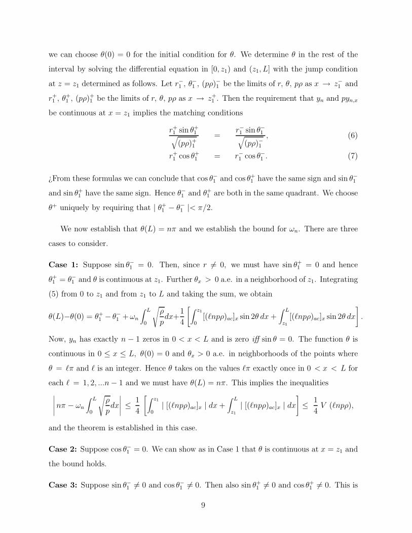
we can choose θ(0) = 0 for the initial condition for θ. We determine θ in the rest of the

interval by solving the differential equation in [0, z1) and (z1, L] with the jump condition

at z = z1 determined as follows. Let r−1 , θ−1 , (pρ)−1 be the limits of r, θ, pρ as x → z−1 and

r+1 , θ+

1 , (pρ)+1 be the limits of r, θ, pρ as x → z+

1 . Then the requirement that yn and pyn,x

be continuous at x = z1 implies the matching conditions

r+1 sin θ+

1√

(pρ)+1

=r−1 sin θ−1√

(pρ)−1, (6)

r+1 cos θ+

1 = r−1 cos θ−1 . (7)

¿From these formulas we can conclude that cos θ−1 and cos θ+1 have the same sign and sin θ−1

and sin θ+1 have the same sign. Hence θ−1 and θ+

1 are both in the same quadrant. We choose

θ+ uniquely by requiring that | θ+1 − θ−1 |< π/2.

We now establish that θ(L) = nπ and we establish the bound for ωn. There are three

cases to consider.

Case 1: Suppose sin θ−1 = 0. Then, since r 6= 0, we must have sin θ+1 = 0 and hence

θ+1 = θ−1 and θ is continuous at z1. Further θx > 0 a.e. in a neighborhood of z1. Integrating

(5) from 0 to z1 and from z1 to L and taking the sum, we obtain

θ(L)−θ(0) = θ+1 − θ−1 + ωn

∫ L

0

√

ρ

pdx+

1

4

[

∫ z1

0[(`npρ)ac]x sin 2θ dx +

∫ L

z1

[(`npρ)ac]x sin 2θ dx

]

.

Now, yn has exactly n − 1 zeros in 0 < x < L and is zero iff sin θ = 0. The function θ is

continuous in 0 ≤ x ≤ L, θ(0) = 0 and θx > 0 a.e. in neighborhoods of the points where

θ = `π and ` is an integer. Hence θ takes on the values `π exactly once in 0 < x < L for

each ` = 1, 2, ...n − 1 and we must have θ(L) = nπ. This implies the inequalities

∣

∣

∣

∣

∣

nπ − ωn

∫ L

0

√

ρ

pdx

∣

∣

∣

∣

∣

≤ 1

4

[

∫ z1

0| [(`npρ)ac]x | dx +

∫ L

z1

| [(`npρ)ac]x | dx

]

≤ 1

4V (`npρ),

and the theorem is established in this case.

Case 2: Suppose cos θ−1 = 0. We can show as in Case 1 that θ is continuous at x = z1 and

the bound holds.

Case 3: Suppose sin θ−1 6= 0 and cos θ−1 6= 0. Then also sin θ+1 6= 0 and cos θ+

1 6= 0. This is

9

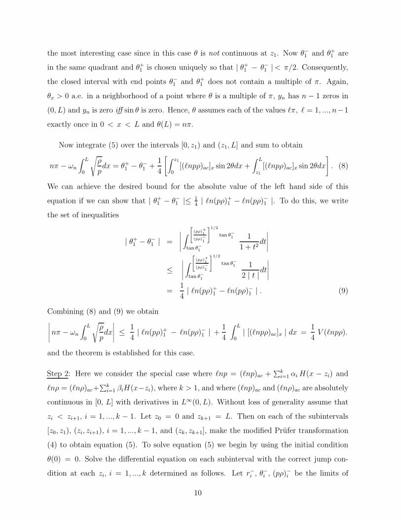
the most interesting case since in this case θ is not continuous at z1. Now θ−1 and θ+1 are

in the same quadrant and θ+1 is chosen uniquely so that | θ+

1 − θ−1 |< π/2. Consequently,

the closed interval with end points θ−1 and θ+1 does not contain a multiple of π. Again,

θx > 0 a.e. in a neighborhood of a point where θ is a multiple of π, yn has n − 1 zeros in

(0, L) and yn is zero iff sin θ is zero. Hence, θ assumes each of the values `π, ` = 1, ..., n−1

exactly once in 0 < x < L and θ(L) = nπ.

Now integrate (5) over the intervals [0, z1) and (z1, L] and sum to obtain

nπ − ωn

∫ L

0

√

ρ

pdx = θ+

1 − θ−1 +1

4

[

∫ z1

0[(`npρ)ac]x sin 2θdx +

∫ L

z1

[(`npρ)ac]x sin 2θdx

]

. (8)

We can achieve the desired bound for the absolute value of the left hand side of this

equation if we can show that | θ+1 − θ−1 |≤ 1

4| `n(pρ)+

1 − `n(pρ)−1 |. To do this, we write

the set of inequalities

| θ+1 − θ−1 | =

∣

∣

∣

∣

∣

∫

[

(pρ)+1

(pρ)−1

]1/2

tan θ−1

tan θ−1

1

1 + t2dt

∣

∣

∣

∣

∣

≤∣

∣

∣

∣

∣

∫

[

(pρ)+1

(pρ)−1

]1/2

tan θ−1

tan θ−1

1

2 | t |dt

∣

∣

∣

∣

∣

=1

4| `n(pρ)+

1 − `n(pρ)−1 | . (9)

Combining (8) and (9) we obtain∣

∣

∣

∣

∣

nπ − ωn

∫ L

0

√

ρ

pdx

∣

∣

∣

∣

∣

≤ 1

4| `n(pρ)+

1 − `n(pρ)−1 | +1

4

∫ L

0| [(`npρ)ac]x | dx =

1

4V (`npρ).

and the theorem is established for this case.

Step 2: Here we consider the special case where `np = (`np)ac +∑k

i=1 αi H(x − zi) and

`nρ = (`nρ)ac+∑k

i=1 βiH(x−zi), where k > 1, and where (`np)ac and (`nρ)ac are absolutely

continuous in [0, L] with derivatives in L∞(0, L). Without loss of generality assume that

zi < zi+1, i = 1, ..., k − 1. Let z0 = 0 and zk+1 = L. Then on each of the subintervals

[z0, z1), (zi, zi+1), i = 1, ..., k − 1, and (zk, zk+1], make the modified Prufer transformation

(4) to obtain equation (5). To solve equation (5) we begin by using the initial condition

θ(0) = 0. Solve the differential equation on each subinterval with the correct jump con-

dition at each zi, i = 1, ..., k determined as follows. Let r−i , θ−i , (pρ)−i be the limits of

10

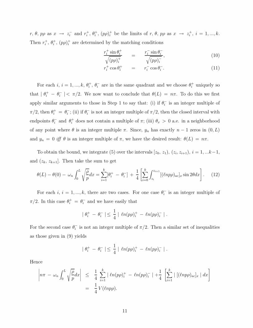
r, θ, pρ as x → z−i and r+i , θ+

i , (pρ)+i be the limits of r, θ, pρ as x → z+

i , i = 1, ..., k.

Then r+i , θ+

i , (pρ)+i are determined by the matching conditions

r+i sin θ+

i√

(pρ)+i

=r−i sin θ−i√

(pρ)−i, (10)

r+i cos θ+

i = r−i cos θ−i . (11)

For each i, i = 1, ..., k, θ+i , θ−i are in the same quadrant and we choose θ+

i uniquely so

that | θ+i − θ−i |< π/2. We now want to conclude that θ(L) = nπ. To do this we first

apply similar arguments to those in Step 1 to say that: (i) if θ−i is an integer multiple of

π/2, then θ+i = θ−i ; (ii) if θ−i is not an integer multiple of π/2, then the closed interval with

endpoints θ−i and θ+i does not contain a multiple of π; (iii) θx > 0 a.e. in a neighborhood

of any point where θ is an integer multiple π. Since, yn has exactly n − 1 zeros in (0, L)

and yn = 0 iff θ is an integer multiple of π, we have the desired result: θ(L) = nπ.

To obtain the bound, we integrate (5) over the intervals [z0, z1), (zi, zi+1), i = 1, ...k−1,

and (zk, zk+1]. Then take the sum to get

θ(L) − θ(0) − ωn

∫ L

0

√

ρ

pdx =

k∑

i=1

[θ+i − θ−i ] +

1

4

[

k∑

i=0

∫ zi+1

zi

[(`npρ)ac]x sin 2θdx

]

. (12)

For each i, i = 1, ..., k, there are two cases. For one case θ−i is an integer multiple of

π/2. In this case θ+i = θ−i and we have easily that

| θ+i − θ−i | ≤ 1

4| `n(pρ)+

i − `n(pρ)−i | .

For the second case θ−i is not an integer multiple of π/2. Then a similar set of inequalities

as those given in (9) yields

| θ+i − θ−i | ≤ 1

4| `n(pρ)+

i − `n(pρ)−i | .

Hence∣

∣

∣

∣

∣

nπ − ωn

∫ L

0

√

ρ

pdx

∣

∣

∣

∣

∣

≤ 1

4

k∑

i=1

| `n(pρ)+i − `n(pρ)−i | +

1

4

[

k∑

i=1

| [(`npρ)ac]x | dx

]

=1

4V (`npρ).

11

and the theorem is established for this case.

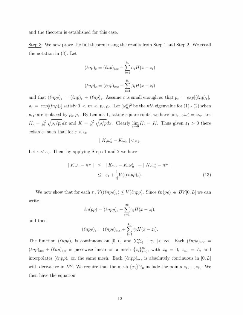
Step 3: We now prove the full theorem using the results from Step 1 and Step 2. We recall

the notation in (3). Let

(`np)ε = (`np)acε +kε∑

i=1

αiH(x − zi)

(`nρ)ε = (`nρ)acε +kε∑

i=1

βiH(x − zi)

and that (`npρ)ε = (`np)ε + (`nρ)ε. Assume ε is small enough so that pε = exp[(`np)ε],

ρε = exp[(lnρ)ε] satisfy 0 < m < pε, ρε. Let (ωεn)2 be the nth eigenvalue for (1) - (2) when

p, ρ are replaced by pε, ρε. By Lemma 1, taking square roots, we have limε→0 ωεn = ωn. Let

Kε =∫ L0

√

ρε/pεdx and K =∫ L0

√

ρ/pdx. Clearly limε→0

Kε = K. Thus given ε1 > 0 there

exists ε0 such that for ε < ε0

| Kεωεn − Kωn |< ε1.

Let ε < ε0. Then, by applying Steps 1 and 2 we have

| Kωn − nπ | ≤ | Kωn − Kεωεn | + | Kεω

εn − nπ |

≤ ε1 +1

4V ((`npρ)ε). (13)

We now show that for each ε , V ((`npρ)ε) ≤ V (`npρ). Since `n(pρ) ∈ BV [0, L] we can

write

`n(pρ) = (`npρ)c +∞∑

i=1

γiH(x − zi),

and then

(`npρ)ε = (`npρ)acε +kε∑

i=1

γiH(x − zi).

The function (`npρ)c is continuous on [0, L] and∑∞

i=1 | γi |< ∞. Each (`npρ)acε =

(`np)acε + (`nρ)acε is piecewise linear on a mesh {xi}nε

i=0, with x0 = 0, xnε = L, and

interpolates (`npρ)c on the same mesh. Each (`npρ)acε is absolutely continuous in [0, L]

with derivative in L∞. We require that the mesh {xi}nεi=0 include the points z1, ..., zkε. We

then have the equation

12

V (`npρ)ε

=nε∑

i=1

| (`npρ)ε(x−i ) − (`n pρ)ε(x

+i−1) | +

nε∑

i=1

| (`npρ)ε(x+i ) − (`npρ)ε(x

−i ) |

=nε∑

i=1

| (`npρ)acε(x−i ) − (`npρ)acε(x

+i−1) | +

kε∑

i=1

| (`npρ)(zi) − limx→z−i

(`npρ)(x) |

=nε∑

i=1

| (`npρ)c(x−i ) − (`npρ)c(x

+i−1) | +

kε∑

i=1

| (`npρ)(zi) − limx→z−i

(`npρ)(x) |

≤ V (`npρ)

Inserting this inequality into (13) we obtain

|K ωn − n π | ≤ ε1 +1

4V ((`npρ))

for all ε1 > 0. Let ε1 → 0 and the proof is complete. •

It remains to prove Lemma 1. We will do this after presenting our next three theorems

and after presenting some numerical experiments.

Our bound in Theorem 1 is sharp for functions p, ρ that are continuous and of bounded

variation. To show this we construct an explicit example. This is done in Appendices

A and B. There we construct a specific ’Cantor’ function in Appendix A and use it in

Appendix B to establish the following theorem.

Theorem 2: There exist pairs of continuous coefficients, pq, ρq ∈ BV [0, 1], and eigenvalues,

(ωnq)2, for (1)-(2) that satisfy

K =∫ 1

0

√

ρq/pq dx = 1,1

4V (ln pqρq) =

1

2,

for all q = 1, 2, ... and

|Kωnq − nqπ | − 1

4V (ln pqρq) ≤ 4π2

92q+2,

implying

13

limq→∞ | ωnq − nqπ | − 1

4V (ln pqρq) = 0.

Now consider the case where p and ρ can have discontinuities. We observe in our

numerical experiments, with piecewise constant p and ρ, that the bound is often not sharp.

In our computations it was possible to obtain relative errors, i.e. values of

|ωn

∫ L0

√

ρ/pdx−nπ| − 14V (`npρ)×

[

14V (`npρ)

]−1, as small as 10−4 or smaller. To do this,

however, the jumps at the discontinuities, while not zero, might have to be extremely small.

Below we give histograms for three more typical examples. In each example the interval

[−A, A] where A = maxn |ωn K − nπ|, K =∫ L0

√

ρ/pdx is divided into 20 subintervals.

The vertical dashed lines, at ±B, mark the bound B = 14V (`npρ).

To compute we used the following formula. Letting ρ ≡ 1, z0 = 0, z3 = L, p(x) = b2i

for zi−1 ≤ x < zi, i = 1, 2, 3, and p(L) = b23, then ω satisfies

sin(ωK) =b2 − b1

b2 + b1sin

(

ω(

K − 2z1 − z0

b1

))

+b2 − b3

b2 + b3sin

(

ω(

K − 2z3 − z2

b3

))

+b2 − b1

b2 + b1· b2 − b3

b2 + b3sin

(

ω(

K − 2z2 − z1

b2

))

.

Setting b2 = b3 gives the formula for one discontinuity, see [H], [Wi]. In all our examples,

z1 = (1/2) −√

2/8, z2 = z1 + 2/√

8 + 2/√

5, and L = z2 + 1 − 1/√

5.

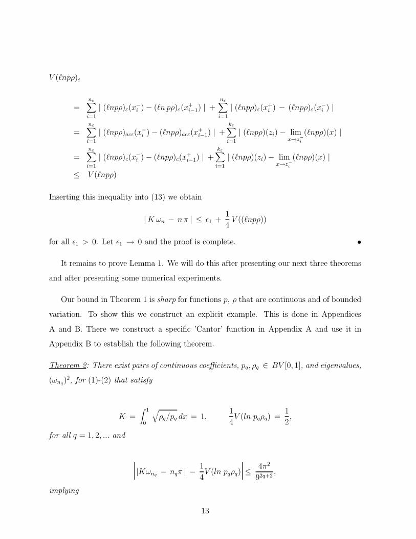
Figure 1 corresponds to b1 = 1, b2 = b3 = 2. For this case 14V (`npρ) = B = .34657

14

and the largest difference |ωn K − n π| is A = .33984.

Figure 1. Histogram for 60,000 values of ωnK − nπ where

A = .33984 and B = .34657.

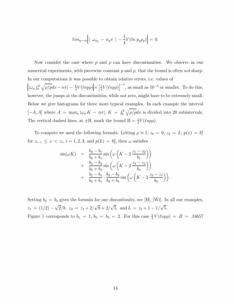
Figures 2 and 3 are histograms for cases where p has two discontinuities. Figure 2 has

b1 = 1, b2 = 2.1, b3 = 2, so that the second jump discontinuity is quite small. Here

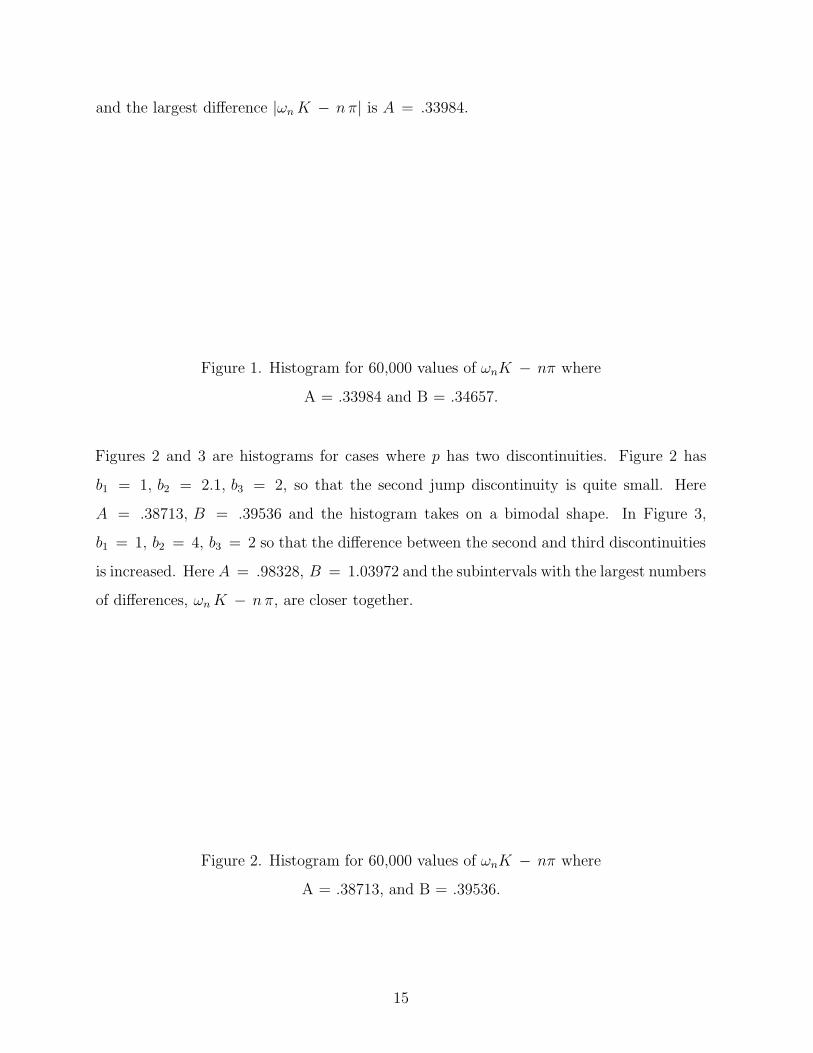
A = .38713, B = .39536 and the histogram takes on a bimodal shape. In Figure 3,

b1 = 1, b2 = 4, b3 = 2 so that the difference between the second and third discontinuities

is increased. Here A = .98328, B = 1.03972 and the subintervals with the largest numbers

of differences, ωn K − n π, are closer together.

Figure 2. Histogram for 60,000 values of ωnK − nπ where

A = .38713, and B = .39536.

15

Figure 3. Histogram for 60,000 values of ωnK − nπ where

A = .98328, and B = 1.03972.

These computations suggest that the bound can be improved when p, ρ are piecewise

constant functions. In fact we can prove

Theorem 3: (Bounds for the eigenvalues). Let p, ρ be piecewise constant positive functions

continuous from the right and satisfying 0 < m < p, ρ for all 0 ≤ x ≤ L. Let ω2n be the

nth eigenvalue, n = 1, 2, ... for (1)-(2). Let zi be the positions of the discontinuities and let

(pρ)+i = limx→z+

i(pρ), (pρ)−i = limx→z−i

(pρ), i = 1, 2, ...k. Then

| ωn

∫ L

0

√

ρ/p dx − nπ |≤k∑

i=1

arcsin[

√

(pρ)+i −

√

(pρ)−i ) /(

√

(pρ)+i +

√

(pρ)−i

)]

where arcsin refers to the principal value.

Proof of Theorem 3: Following the arguments given in the proof of Theorem 1, using the

Prufer transformation (4) and letting θ+i = limx→z+

iθ, θ−i = limx→z−i

θ, we observe that

| ωn

∫ L

0

√

ρ/p dx − nπ |≤k∑

i=1

| θ+i − θ−i |

where

16

| θ+i − θ−i | =

∫

[

(pρ)+i

(pρ)−i

]1/2

tan θ−i

tan θ−i

1

1 + t2dt

= arctan

[

(pρ)+i

(pρ)−i

]1/2

tan θ−i

− arctan(tan θ−i )

< arctan

[

(pρ)+i

(pρ)+i

]1/4

− arctan

[

(pρ)+i

(pρ)−i

]−1/4

= arcsin({

[

(pρ)+i /(pρ)−i

]1/2 − 1}

/{

[

(pρ)+i /(pρ)−i

]1/2+ 1

})

= arcsin({

[

(pρ)+i

]1/2 −[

(pρ)−i]1/2

}

/{

[

(pρ)+i

]1/2+[

(pρ)−i]1/2

})

< `n[

(pρ)+i /(pρ)−i

]1/4(14)

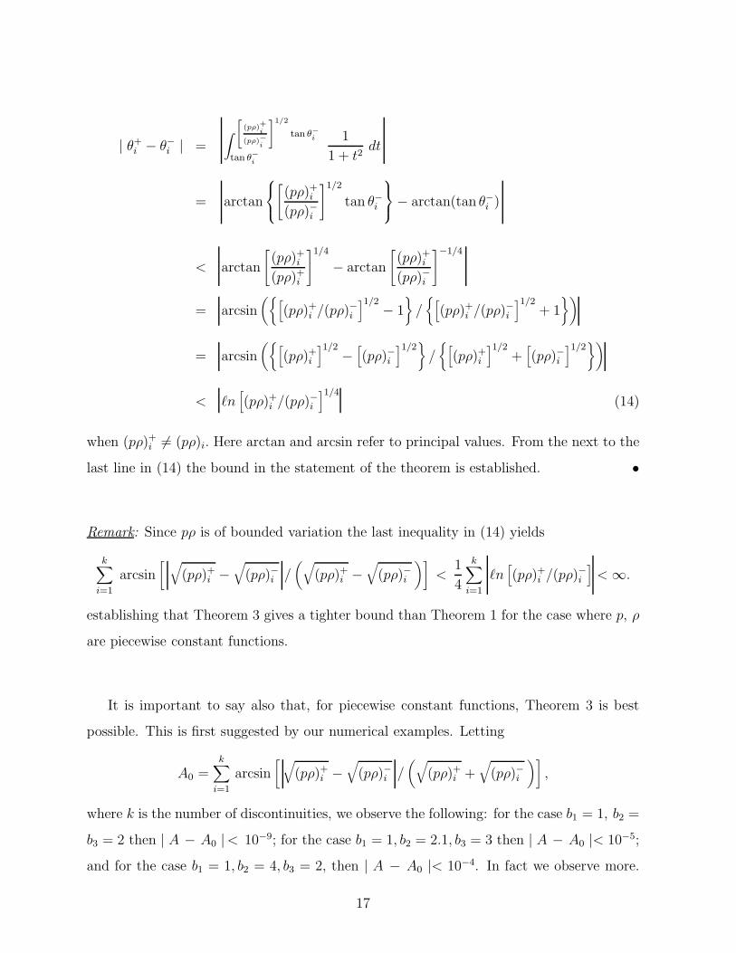
when (pρ)+i 6= (pρ)i. Here arctan and arcsin refer to principal values. From the next to the

last line in (14) the bound in the statement of the theorem is established. •

Remark: Since pρ is of bounded variation the last inequality in (14) yields

k∑

i=1

arcsin[

√

(pρ)+i −

√

(pρ)−i /(

√

(pρ)+i −

√

(pρ)−i

)]

<1

4

k∑

i=1

`n[

(pρ)+i /(pρ)−i

]

< ∞.

establishing that Theorem 3 gives a tighter bound than Theorem 1 for the case where p, ρ

are piecewise constant functions.

It is important to say also that, for piecewise constant functions, Theorem 3 is best

possible. This is first suggested by our numerical examples. Letting

A0 =k∑

i=1

arcsin[

√

(pρ)+i −

√

(pρ)−i /(

√

(pρ)+i +

√

(pρ)−i

)]

,

where k is the number of discontinuities, we observe the following: for the case b1 = 1, b2 =

b3 = 2 then | A − A0 |< 10−9; for the case b1 = 1, b2 = 2.1, b3 = 3 then | A − A0 |< 10−5;

and for the case b1 = 1, b2 = 4, b3 = 2, then | A − A0 |< 10−4. In fact we observe more.

17

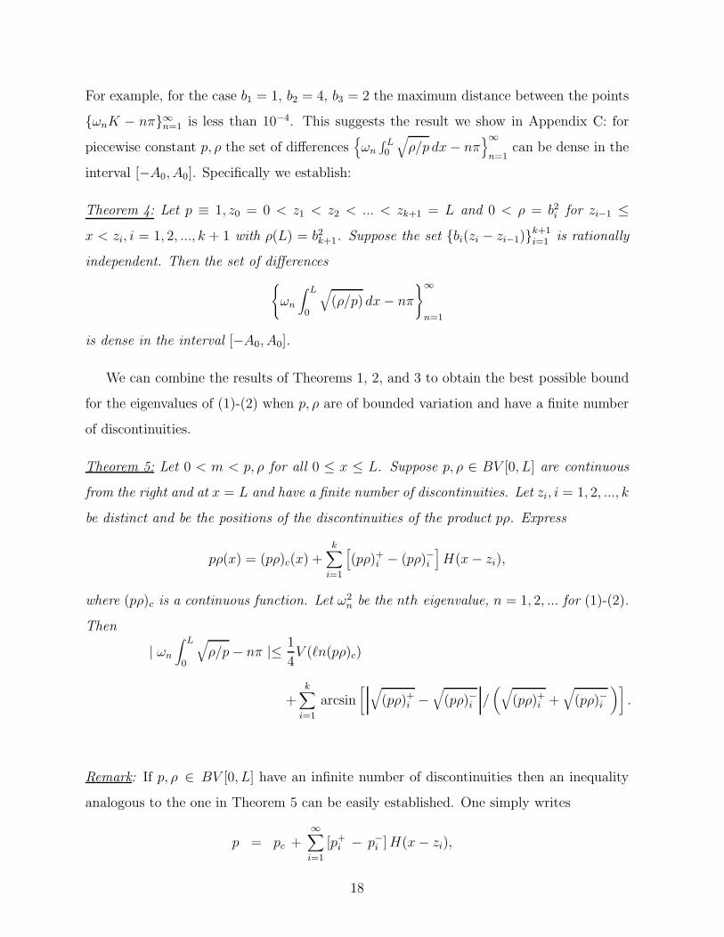
For example, for the case b1 = 1, b2 = 4, b3 = 2 the maximum distance between the points

{ωnK − nπ}∞n=1 is less than 10−4. This suggests the result we show in Appendix C: for

piecewise constant p, ρ the set of differences{

ωn

∫ L0

√

ρ/p dx − nπ}∞

n=1can be dense in the

interval [−A0, A0]. Specifically we establish:

Theorem 4: Let p ≡ 1, z0 = 0 < z1 < z2 < ... < zk+1 = L and 0 < ρ = b2i for zi−1 ≤

x < zi, i = 1, 2, ..., k + 1 with ρ(L) = b2k+1. Suppose the set {bi(zi − zi−1)}k+1

i=1 is rationally

independent. Then the set of differences

{

ωn

∫ L

0

√

(ρ/p) dx − nπ

}∞

n=1

is dense in the interval [−A0, A0].

We can combine the results of Theorems 1, 2, and 3 to obtain the best possible bound

for the eigenvalues of (1)-(2) when p, ρ are of bounded variation and have a finite number

of discontinuities.

Theorem 5: Let 0 < m < p, ρ for all 0 ≤ x ≤ L. Suppose p, ρ ∈ BV [0, L] are continuous

from the right and at x = L and have a finite number of discontinuities. Let zi, i = 1, 2, ..., k

be distinct and be the positions of the discontinuities of the product pρ. Express

pρ(x) = (pρ)c(x) +k∑

i=1

[

(pρ)+i − (pρ)−i

]

H(x − zi),

where (pρ)c is a continuous function. Let ω2n be the nth eigenvalue, n = 1, 2, ... for (1)-(2).

Then

| ωn

∫ L

0

√

ρ/p − nπ |≤ 1

4V (`n(pρ)c)

+k∑

i=1

arcsin[

√

(pρ)+i −

√

(pρ)−i /(

√

(pρ)+i +

√

(pρ)−i

)]

.

Remark: If p, ρ ∈ BV [0, L] have an infinite number of discontinuities then an inequality

analogous to the one in Theorem 5 can be easily established. One simply writes

p = pc +∞∑

i=1

[p+i − p−i ] H(x − zi),

18

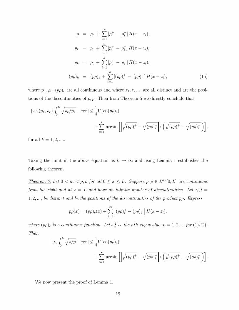
ρ = ρc +∞∑

i=1

[ρ+i − ρ−

i ] H(x − zi),

pk = pc +k∑

i=1

[p+i − p−i ] H(x − zi),

ρk = ρc +k∑

i=1

[ρ+i − ρ−

i ] H(x − zi),

(pρ)k = (pρ)c +k∑

i=1

[(pρ)+i − (pρ)−i ] H(x− zi), (15)

where pc, ρc, (pρ)c are all continuous and where z1, z2, ... are all distinct and are the posi-

tions of the discontinuities of p, ρ. Then from Theorem 5 we directly conclude that

| ωn(pk, ρk)∫ L

0

√

ρk/pk − nπ |≤ 1

4V (`n(pρ)c)

+k∑

i=1

arcsin[

√

(pρ)+i −

√

(pρ)−i /(

√

(pρ)+i +

√

(pρ)−i

)]

.

for all k = 1, 2, .....

Taking the limit in the above equation as k → ∞ and using Lemma 1 establishes the

following theorem

Theorem 6: Let 0 < m < p, ρ for all 0 ≤ x ≤ L. Suppose p, ρ ∈ BV [0, L] are continuous

from the right and at x = L and have an infinite number of discontinuities. Let zi, i =

1, 2, ..., be distinct and be the positions of the discontinuities of the product pρ. Express

pρ(x) = (pρ)c(x) +∞∑

i=1

[

(pρ)+i − (pρ)−i

]

H(x − zi),

where (pρ)c is a continuous function. Let ω2n be the nth eigenvalue, n = 1, 2, ... for (1)-(2).

Then

| ωn

∫ L

0

√

ρ/p − nπ |≤ 1

4V (`n(pρ)c)

+∞∑

i=1

arcsin[

√

(pρ)+i −

√

(pρ)−i /(

√

(pρ)+i +

√

(pρ)−i

)]

.

We now present the proof of Lemma 1.

19

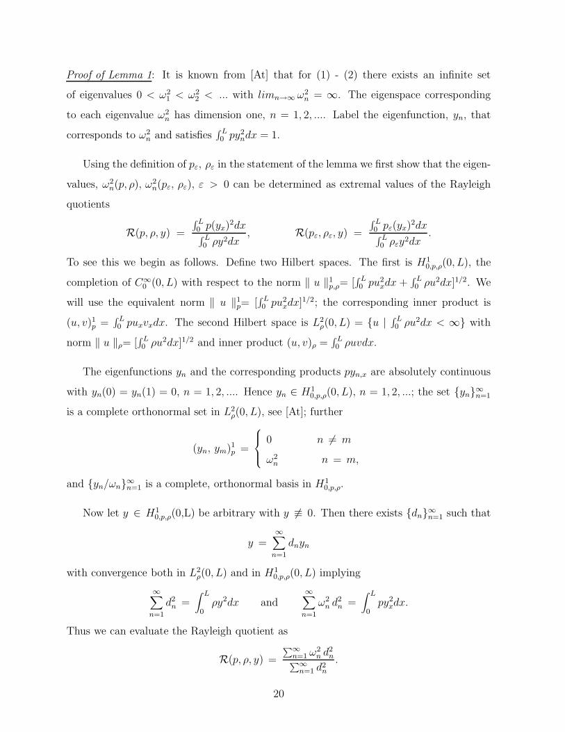
Proof of Lemma 1: It is known from [At] that for (1) - (2) there exists an infinite set

of eigenvalues 0 < ω21 < ω2

2 < ... with limn→∞ ω2n = ∞. The eigenspace corresponding

to each eigenvalue ω2n has dimension one, n = 1, 2, .... Label the eigenfunction, yn, that

corresponds to ω2n and satisfies

∫ L0 py2

ndx = 1.

Using the definition of pε, ρε in the statement of the lemma we first show that the eigen-

values, ω2n(p, ρ), ω2

n(pε, ρε), ε > 0 can be determined as extremal values of the Rayleigh

quotients

R(p, ρ, y) =

∫ L0 p(yx)

2dx∫ L0 ρy2dx

, R(pε, ρε, y) =

∫ L0 pε(yx)

2dx∫ L0 ρεy2dx

.

To see this we begin as follows. Define two Hilbert spaces. The first is H10,p,ρ(0, L), the

completion of C∞0 (0, L) with respect to the norm ‖ u ‖1

p,ρ= [∫ L0 pu2

xdx +∫ L0 ρu2dx]1/2. We

will use the equivalent norm ‖ u ‖1p= [

∫ L0 pu2

xdx]1/2; the corresponding inner product is

(u, v)1p =

∫ L0 puxvxdx. The second Hilbert space is L2

ρ(0, L) = {u | ∫ L0 ρu2dx < ∞} with

norm ‖ u ‖ρ= [∫ L0 ρu2dx]1/2 and inner product (u, v)ρ =

∫ L0 ρuvdx.

The eigenfunctions yn and the corresponding products pyn,x are absolutely continuous

with yn(0) = yn(1) = 0, n = 1, 2, .... Hence yn ∈ H10,p,ρ(0, L), n = 1, 2, ...; the set {yn}∞n=1

is a complete orthonormal set in L2ρ(0, L), see [At]; further

(yn, ym)1p =

0 n 6= m

ω2n n = m,

and {yn/ωn}∞n=1 is a complete, orthonormal basis in H10,p,ρ.

Now let y ∈ H10,p,ρ(0,L) be arbitrary with y 6≡ 0. Then there exists {dn}∞n=1 such that

y =∞∑

n=1

dnyn

with convergence both in L2ρ(0, L) and in H1

0,p,ρ(0, L) implying

∞∑

n=1

d2n =

∫ L

0ρy2dx and

∞∑

n=1

ω2n d2

n =∫ L

0py2

xdx.

Thus we can evaluate the Rayleigh quotient as

R(p, ρ, y) =

∑∞n=1 ω2

n d2n

∑∞n=1 d2

n

.

20

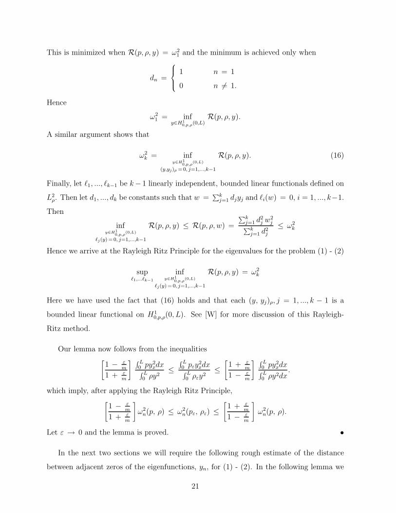
This is minimized when R(p, ρ, y) = ω21 and the minimum is achieved only when

dn =

1 n = 1

0 n 6= 1.

Hence

ω21 = inf

y∈H10,p,ρ(0,L)

R(p, ρ, y).

A similar argument shows that

ω2k = inf

y∈H10,p,ρ

(0,L)

(y,yj)ρ =0, j=1,...,k−1

R(p, ρ, y). (16)

Finally, let `1, ..., `k−1 be k− 1 linearly independent, bounded linear functionals defined on

L2ρ. Then let d1, ..., dk be constants such that w =

∑kj=1 djyj and `i(w) = 0, i = 1, ..., k−1.

Then

infy∈H1

0,p,ρ(0,L)

`j(y) =0, j=1,...,k−1

R(p, ρ, y) ≤ R(p, ρ, w) =

∑kj=1 d2

j w2j

∑kj=1 d2

j

≤ ω2k

Hence we arrive at the Rayleigh Ritz Principle for the eigenvalues for the problem (1) - (2)

sup`1,...`k−1

infy∈H1

0,p,ρ(0,L)

`j(y) = 0, j=1,...,k−1

R(p, ρ, y) = ω2k

Here we have used the fact that (16) holds and that each (y, yj)ρ, j = 1, ..., k − 1 is a

bounded linear functional on H10,p,ρ(0, L). See [W] for more discussion of this Rayleigh-

Ritz method.

Our lemma now follows from the inequalities[

1 − εm

1 + εm

]∫ L0 py2

xdx∫ L0 ρy2

≤∫ L0 pεy

2xdx

∫ L0 ρεy2

≤[

1 + εm

1 − εm

]∫ L0 py2

xdx∫ L0 ρy2dx

.

which imply, after applying the Rayleigh Ritz Principle,[

1 − εm

1 + εm

]

ω2n(p, ρ) ≤ ω2

n(pε, ρε) ≤[

1 + εm

1 − εm

]

ω2n(p, ρ).

Let ε → 0 and the lemma is proved. •

In the next two sections we will require the following rough estimate of the distance

between adjacent zeros of the eigenfunctions, yn, for (1) - (2). In the following lemma we

21

show that when n → ∞, the distance between adjacent zeros of yn goes to zero. Before

we state the lemma we remind the reader that a function of bounded variation is always

bounded.

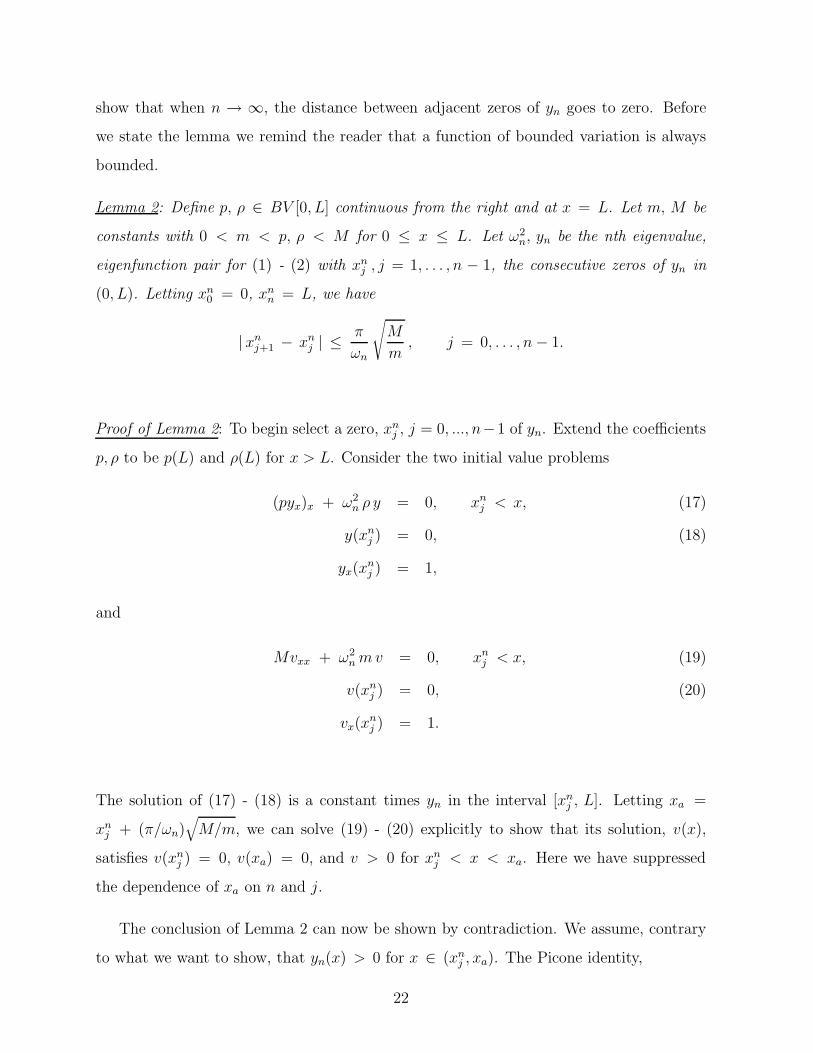
Lemma 2: Define p, ρ ∈ BV [0, L] continuous from the right and at x = L. Let m, M be

constants with 0 < m < p, ρ < M for 0 ≤ x ≤ L. Let ω2n, yn be the nth eigenvalue,

eigenfunction pair for (1) - (2) with xnj , j = 1, . . . , n − 1, the consecutive zeros of yn in

(0, L). Letting xn0 = 0, xn

n = L, we have

| xnj+1 − xn

j | ≤π

ωn

√

M

m, j = 0, . . . , n − 1.

Proof of Lemma 2: To begin select a zero, xnj , j = 0, ..., n−1 of yn. Extend the coefficients

p, ρ to be p(L) and ρ(L) for x > L. Consider the two initial value problems

(pyx)x + ω2n ρ y = 0, xn

j < x, (17)

y(xnj ) = 0, (18)

yx(xnj ) = 1,

and

Mvxx + ω2n m v = 0, xn

j < x, (19)

v(xnj ) = 0, (20)

vx(xnj ) = 1.

The solution of (17) - (18) is a constant times yn in the interval [xnj , L]. Letting xa =

xnj + (π/ωn)

√

M/m, we can solve (19) - (20) explicitly to show that its solution, v(x),

satisfies v(xnj ) = 0, v(xa) = 0, and v > 0 for xn

j < x < xa. Here we have suppressed

the dependence of xa on n and j.

The conclusion of Lemma 2 can now be shown by contradiction. We assume, contrary

to what we want to show, that yn(x) > 0 for x ∈ (xnj , xa). The Picone identity,

22

see [I, p.226],

(

pyn,xv2

yn− Mvvx

)

x+ p

(

vx − vyn,x

yn

)2

+ (M − p)v2x + ω2

n(ρ − m)v2 = 0.

is valid, a.e., in [xnj , xa]. Since (pyn,xv

2/yn) − Mvvx is absolutely continuous in [xnj , xa], we

can integrate the identity from xnj to xa to obtain

∫ xa

xnj

{

p[

vx − vyn,x

yn

]2

+ (M − p)v2x + ω2

n(ρ − m)v2

}

dx = 0.

Then the contradiction follows from the facts that m < p, ρ < M and 0 < v in (xnj , xa);

the conclusion of Lemma 2 follows. •

Section 3: Uniqueness Theorems

In this section we present uniqueness results for the inverse nodal problem for two special

cases of problem (1) - (2). For the first case p ≡ 1 and ρ is variable and unknown on [0, L].

For the second case, ρ ≡ 1 and p is variable and unknown on [0, L]. We show for each case

that the unknown variable coefficient, p or ρ, is determined uniquely (up to a multiplicative

constant) at every point of continuity by a dense subset of nodal positions. If p and ρ are

smooth, see [McL], [HMcL1] and [HMcL2], then the dense subset is completely arbitrary.

In this rough coefficient case our assumptions are stronger. We require that if xnj is in the

dense subset then either xnj−1 or xn

j+1 is also in the dense subset. We present the following

two uniqueness results.

Theorem 7: In (1) - (2) let p ≡ 1, ρ ∈ BV [0, L], continuous from the right and at x = L.

Suppose there exists a constant m with 0 < m < ρ for 0 ≤ x ≤ L. Then ρ is uniquely

determined up to one multiplicative constant by a dense subset of pairs of nodal positions,

xnj , xn

j+1.

Proof of Theorem 7: Let ρ1, ρ2 both satisfy the hypotheses of the theorem. Suppose that

for a dense subset of pairs of nodal positions xnj (ρ1) = xn

j (ρ2) and xnj+1(ρ1) = xn

j+1(ρ2).

We will show that there exists a constant R > 0 such that ρ1/ρ2 ≡ R at every point of

continuity of ρ1 and ρ2.

23

To do this let x ∈ [0, L] be a point of continuity of both ρ1 and ρ2. Let[

xn′

j(n′), xn′

j(n′)+1

]

,

n′ = 1, 2, ..., be a subset of the closed intervals defined by the given pairs of nodal posi-

tions and satisfying x = limn′→∞ xn′

j(n′). For each n′, n′ = 1, 2, ... let wn′, yn′ be the n′th

eigenfunctions for the problem (1) - (2) with p ≡ 1 and ρ = ρ1 or ρ = ρ2 respectively.

Then ω2n′(ρ1), wn′ and ω2

n′(ρ2), yn′ are the first eigenvalue, eigenfunction pairs for

wxx + ω2 ρ1 w = 0, (21)

w(xj) = w(xj+1) = 0, (22)

and

yxx + ω2 ρ2 y = 0, (23)

y(xj) = y(xj+1) = 0, (24)

respectively. Here we have suppressed the dependency of the nodal positions on n′.

Substitute w = wn′ in (21) and y = yn′ in (23). Multiply equation (21) by yn′ and

equation (23) by wn′. Subtract the two equations, integrate from xj to xj+1 and divide by

ω2n′(ρ1). The result is

∫ xj+1

xj

[

ρ1 −ω2

n′(ρ2)

ω2n′(ρ1)

ρ2

]

wn′yn′dx = 0.

Without loss we may assume that wn′yn′ > 0 for xj < x < xj+1. Hence there exists

x′j , x

′′j ∈ (xj , xj+1) with

[

ρ1 −ω2

n′(ρ2)

ω2n′(ρ1)

ρ2

] ∣

∣

∣

∣

∣

x=x′

j

≥ 0

[

ρ1 −ω2

n′(ρ2)

ω2n′(ρ1)

ρ2

] ∣

∣

∣

∣

∣

x=x′′

j

≤ 0

Recall that j = j(n′). Since ρ is in BV [0, L] it is bounded above. Lemma 2 can be applied

to show that xn′

j(n′) − xn′

j(n′)+1 → 0 as n′ → ∞. Hence x′j → x, x′′

j → x as n′ → ∞.

¿From Theorem 1 we conclude that limn′→∞ ω2n′(ρ2)/ω

2n′(ρ1) exists. Label the limit, R.

Then in both of the above two inequalities let n′ → ∞ to obtain

(ρ1 − Rρ2) (x) = 0.

24

This shows that ρ1 − Rρ2 = 0 at every point of continuity of ρ1 and ρ2. Since ρ1 and

ρ2 each can have only a countable number of discontinuities and are both continuous from

the right, the equation, ρ1 − Rρ2 = 0, holds for all x ∈ [0, L]. The theorem is proved. •

Theorem 8: In (1) and (2) let ρ ≡ 1, p ∈ BV [0, L], continuous from the right and at

x = L. Suppose there exists a constant m with 0 < m < p for 0 ≤ x ≤ L. Then p

is uniquely determined, up to one multiplicative constant, from a dense subset of pairs of

nodal positions xnj , xn

j+1.

Proof of Theorem 8: Let p1, p2 satisfy the hypotheses of the theorem. Suppose that for

a dense subset of pairs of nodal positions xnj (p1) = xn

j (p2) and xnj+1(p1) = xn

j+1(p2). To

establish the theorem we will show that there exists a constant R > 0 such that p1/p2 ≡ R

at every point of continuity of p1 and p2.

To do this let x ∈ [0, L] be a point of continuity of both p1 and p2. Let[

xn′

j(n′), xn′

j(n′)+1

]

be

a subset of the closed intervals defined by the given pairs of nodal positions and satisfying

x = limn′→∞ xn′

j(n′). For each n′, let wn′, yn′ be the n′th eigenfunctions for the problem (1)

- (2) with ρ ≡ 1 and p = p1 or p = p2, respectively. Then ω2n′(p1), wn′ and ω2

n′(p2), yn′ are

the first eigenvalue, eigenfunction pairs for the eigenvalue problems

(p1 wx)x + ω2 w = 0, (25)

w(xj) = w(xj+1) = 0, (26)

and

(p2 yx)x + ω2 y = 0, (27)

y(xj) = y(xj+1) = 0, (28)

respectively. Here again we have suppressed the dependency of the nodal positions on n′.

Substitute w = wn′ in (25) and y = yn′ in (27). Then multiply (25) by wn′ and (27)

by [w2n′/yn′] × [ω2

n′(p1)/ω2n′(p2)], subtract the first resultant equation from the second and

integrate from xj to xj+1. This yields the equation

∫ xj+1

xj

[

p1 −ω2

n′(p1)

ω2n′(p2)

p2

]

(wn′,x)2 dx +

∫ xj+1

xj

[

ω2n′(p1)

ω2n′(p2)

p2

] [

wn′,xyn′ − yn′,xwn′

yn′

]2

dx = 0.

25

Again we suppress the dependence of xj , xj+1 on n′. We also delay the argument that

the ratio, wn′/yn′, is bounded, and hence the integration steps are justified, until the end

of our proof. The second of the above two integrals is non-negative. Hence there exists

x′j ∈ (xj , xj+1) with

(

p1 −ω2

n′(p1)

ω2n′(p2)

p2

)

(x′j) ≤ 0.

To obtain a complimentary inequality multiply (25) by y2n′/wn′ and (27) by yn′ ×

[ω2n′(p1)/ω

2n′(p2)]. Subtract the first resultant equation from the second and integrate from

xj to xj+1. This yields the equation

∫ xj+1

xj

[

p1 −ω2

n′(p1)

ω2n′(p2)

p2

]

(yn′,x)2 dx −

∫ xj+1

xj

p1

[

yn′,xwn′ − wn′,xyn′

wn′

]2

dx = 0.

Again we delay the justification that the ratio, yn′/wn′, is bounded. The second of the

above two integrals is non-negative. Hence there exists x′′j ∈ (xj , xj+1) with

(

p1 −ω2

n′(p1)

ω2n′(p2)

p2

)

(x′′j ) ≥ 0.

Now x′′j → x and x′

j → x as n′ → ∞. Let R = limn′→∞ ω2n′(p1)/ω

2n′(p2). Then taking the

limit as n′ → ∞ we have

p1 = R p2

at every point of continuity of p1 and p2. Since p1 and p2 can have only a countable number

of discontinuities and are both continuous from the right, the theorem will be proved once

we have shown that the ratios, wn′/yn′ and yn′/wn′ are bounded.

The outline of this last demonstration is as follows. Let xj < x < xj+1. Recall that

p1yn′,x and p2wn′,x are absolutely continuous and bounded away from zero in sufficiently

small neighborhoods of any zero of yn and wn respectively. Further there exist xj < x′, x′′ <

x satisfying

yn′(x) =∫ x

xj

yn′,sds =∫ x

xj

1

p2

p2yn′,sds = p2yn′,x(x′)∫ x

xj

1

p2

ds,

wn′(x) =∫ x

xj

wn′,sds =∫ x

xj

1

p1p1wn′,sds = p1wn′,x(x

′′)∫ x

xj

1

p1ds,

from which it follows that wn′/yn′ is bounded as x → x+j . A similar argument applies for

the ratio yn′/wn′ and when x → x−j+1.

26

The proof is complete. •

Remark 1: We remark that the constant R in our proofs can never be determined by the

nodal positions. The reason for this is that we can multiply either p or ρ by a constant

and then if p is changed we would multiply the eigenvalues by the same constant or if ρ

is changed we would divide the eigenvalues by the constant. In either case the eigenvalues

would all change but the eigenfunctions, and hence the nodal positions, would all remain

the same.

Remark 2: In our uniqueness theorems we do not require that the eigenvalues be given as

data. However, if the eigenvalues are known for (1) - (2) when either p ≡ 1 and ρ is

variable or ρ ≡ 1 and p is variable then the multiplicative constant can be determined. In

fact the algorithms in the next section can be adapted to show how to uniquely determine

one variable coefficient at each point of continuity from both the eigenvalues and a dense

subset of pairs of adjacent nodal positions.

Remark 3: It is possible to obtain a dense set of pairs of nodal positions by choosing exactly

one pair from each eigenfunction. See [McL] for this construction for a similar problem.

Remark 4: In our proofs of Theorems 7 and 8 when either p or ρ are assumed known we

choose to assume that they are equal to the constant, 1. The same proof would hold if p in

Theorem 7 and ρ in Theorem 8 are assumed to be known, positive, functions of bounded

variation.

Section 4: Algorithms

In this section we present two sets of algorithms for determining piecewise constant approx-

imations to rough (bounded variation) coefficients from nodal position data. In each of the

algorithms the data is an eigenvalue, ω2n, and all of the nodal positions, xn

j , j = 1, . . . , n−1

27

for the corresponding mode shape or eigenfunction. We choose this data because it can

all be measured when a rod is excited longitudinally or a string is excited transversely at

a natural frequency. An experiment for obtaining these measurements is described in the

introduction.

Our algorithms yield piecewise constant approximates to the unknown coefficient. The

piecewise constant approximates have a special property: when we substitute the nth

approximate in (1) - (2) the corresponding nth eigenvalue, ω2n, and nodal positions, xn

j , j =

1, ...n − 1 are exactly the given data.

In our presentation of the algorithms we let xn0 = 0 and xn

n = L and then suppress the

dependence of the nodal positions on n. Now consider the case where p ≡ 1. Then the

piecewise constant approximate for the coefficient ρ in problem (1) - (2) is given by the

algorithm:

Algorithm A:

ρn =

ρnj+1 =

π2

ω2n(xj+1 − xj)2

xj ≤ x < xj+1, j = 0, . . . , n − 2

ρnn =

π2

ω2n(L − xn−1)2

xn−1 ≤ x ≤ xn = L

Each ρn ∈ BV [0, L]. The following convergence result holds.

Theorem 9: In (1) - (2) let p ≡ 1, ρ ∈ BV [0, L], continuous from the right and at x = L.

Suppose there exists a constant m with 0 < m < ρ for 0 ≤ x ≤ L. Let the nth eigenvalue

ω2n and the n − 1 nodal positions xn

j , j = 1, . . . , n − 1 for the nth eigenfunction be given.

Define ρn as in Algorithm A. Then ρn → ρ pointwise at every point of continuity of ρ.

Furthermore, the total variation V (ρn) ≤ 2V (ρ) for all n.

Proof of Theorem 9: Let yn be the nth eigenfunction for (1) - (2). Let vn be the nth

eigenfunction for

vxx + ω2ρnv = 0. (29)

v(0) = v(L) = 0. (30)

Note that (1) - (2) with p ≡ 1 and (29) - (30) have the same nth eigenvalue, ω2n, and the

same nodal positions for the nth eigenfunction. Because of this property, we can apply the

28

same identities as in the proof of the uniqueness theorem, Theorem 7.

We first show the pointwise convergence. Let x ∈ [0, L) be a point of continuity of ρ.

For each n select j = j(n) so that x ∈ [xnj(n), x

nj(n)+1). Arguing as in the proof of Theorem

7, except that now ωn(ρ) = ωn(ρn) there exists x′

j, x′′j ∈ (xj , xj+1) with

ρ(x′j) ≤ ρn(x) ≤ ρ(x′′

j ).

[We remind the reader that in our notation we suppress the dependence of xj , xj+1, x′j and

x′′j on n.] Now let n → ∞. We have x′

j → x, x′′j → x and

ρ(x) = limn→∞

ρ(x′j) ≤ lim

n→∞ρn(x) ≤ lim

n→∞ρ(x′′

j ) = ρ(x).

Hence ρn(x) → ρ(x). The argument when x = L is a point of continuity is similar.

It remains to show V (ρn) ≤ 2V (ρ) for all n. Clearly

V (ρn) =n−1∑

j=1

|ρnj+1 − ρn

j |.

Now for each j = 1, 2, . . . , n − 1, we know that there exist x′j , x′′

j ∈ (xj , xj+1) and

x′j+1, x′′

j+1 ∈ (xj+1, xj+2) with

ρ(x′j) ≤ ρn

j ≤ ρ(x′′j )

and

ρ(x′j+1) ≤ ρn

j+1 ≤ ρ(x′′j+1)

respectively. This implies that we can choose sj ∈ (xj , xj+1) and tj ∈ (xj+1, xj+2), j =

1, ...n − 1 satisfying

|ρnj+1 − ρn

j | ≤ |ρ(sj) − ρ(tj)|.

Then

V (ρn) =n−1∑

j=1

|ρnj+1 − ρn

j | ≤n−1∑

j=1

|ρ(sj) − ρ(tj)|

=∑

j odd

|ρ(sj) − ρ(tj)| +∑

j even

|ρ(sj) − ρ(tj)|

≤ 2V (ρ)

29

This completes the proof. •

The piecewise constant approximate for problem (1) - (2) when ρ ≡ 1 and p is variable

is given by the algorithm:

Algorithm B:

pn =

pnj+1 =

ω2n(xj+1 − xj)

2

π2xj ≤ x < xj+1, j = 0, . . . , n − 2

pnn =

ω2n(xn − xn−1)

2

π2xn−1 ≤ x ≤ xn = L.

Each pn ∈ BV [0, L]. The following convergence result holds.

Theorem 10: In (1) - (2) let ρ ≡ 1, p ∈ BV [0, 1], continuous from the right and at x = L.

Suppose there exists a constant m with 0 < m < p for 0 ≤ x ≤ L. Let the nth eigenvalue

ω2n and the n − 1 nodal positions xn

j , j = 1, ..., n − 1 for the nth eigenfunction be given.

Define pn as in Algorithm B. Then pn → p pointwise at every point of continuity of p.

Furthermore the total variation V (pn) ≤ 2V (p) for all n.

Proof of Theorem 10: The proof is very similar to the proof of Theorem 9. •Remark: In Theorem 9, it can be shown that there exists an M > 0 so that each ρn satisfies

|ρn| < M and ρn → ρ a.e. In Theorem 10, it can be shown that there exists M > 0 so that

each pn satisfies |pn| < M and pn → p a.e. Hence by the Lebesgue dominated convergence

theorem ρn → ρ and pn → p in Lq(0, L) for any q, 1 ≤ q < ∞. However, no convergence

rate can be given.

Section 5: Numerical Experiments

To test algorithms A, B we must calculate the eigenvalues ω2n and the nodal positions xn

j for

(pyx)x + ω2ρy = 0 with y(0) = y(L) = 0. To do this we use the Prufer transformation

(4). We assume that p, ρ are piecewise smooth functions and use the classical fourth order

Runge-Kutta method to solve equation (5) between the discontinuities with 4000 points

in each subinterval. In all our experiments L = 1. To compute the jump in θ in a stable

manner we consider two cases. If |sin(θ−)| < |cos(θ−)| then

30

θ+ = θ− + tan−1

√

√

√

√

(pρ)+

(pρ)−tan(θ−)

− tan−1[

tan(θ−)]

;

if |cos(θ−)| ≤ |sin(θ−)|, we use

θ+ = θ− +sin(θ−)

|sin(θ−)|

cos−1

cos(θ−)√

(pρ)+

(pρ)−sin2(θ−) + cos2(θ−)

− cos−1[

cos(θ−)]

.

The eigenfrequency ωn is obtained by solving θ(L) = nπ by the IMSL subroutine ZBRENT.

To determine the nodes xnj we solve (5) once more with ω = ωn and determine successive

meshpoints between which (θ + π/2) modπ − π/2 changes sign. Since both θ and θx are

available at the mesh points we find the nodes by inverse interpolation.

We consider two classes of problems

(pyx)x + ω2y = 0 (31)

yxx + ω2ρy = 0, (32)

each with Dirichlet boundary conditions. In Table 1 we give the eigenfrequency and the

nodes for the 10th eigenfunction for (31) and (32) when p = f1 or ρ = f1 where

f1(x) =

√

14

+ 2x 0 ≤ x < 0.375√

3 − 2x 0.375 ≤ x ≤ 1.

Note that the nodes are close when p is small or ρ is large.

31

p = f1 ρ = f1

ω10 31.667945 30.340327

x1 0.074607 0.131772

x2 0.157087 0.248017

x3 0.246160 0.355741

x4 0.340969 0.441698

x5 0.450408 0.528447

x6 0.568081 0.617180

x7 0.682145 0.708204

x8 0.792357 0.801927

x9 0.898426 0.898916

Table 1. Two problems with 9 nodes

Now let en = ρn − ρ and en = pn − p be the errors in algorithms A and B, respectively.

We see from Theorems 9 and 10 that en → 0 a.e. and |en| ≤ 2M . As discussed in

the remark following Theorem 10, it follows that ‖en‖Lq(0,1) → 0 as n → ∞ for any

q ∈ [1,∞). But for p, ρ ∈ BV [0, L], no convergence rate can be given. To study this

problem numerically we set (suppressing the dependence of the nodal positions on n)

xj = (xj + xj−1)/2 and use the discrete L1 norm, the discrete L2 norm and the discrete

maximum norm

‖e‖q =

n∑

j=1

(xj − xj−1)|e(xj)|q

1/q

, q = 1, 2

‖e‖∞ = max1≤j≤n| e(xj)|.

In Table 2 we present the errors when p = f1 and n = 5, 10, 20, 40. The results for ρ = f1

are similar. The main contribution comes from the interval that contains the jump. To

see this we give the truncated errors, obtained by disregarding the interval where p jumps.

The data indicates quadratic convergence away from the discontinuity, which is consistent

with our observations in [HMcL2].

32

n = 5 n = 10 n = 20 n = 40

Discrete L1 error 0.046 0.031 0.011 0.0074

Discrete L2 error 0.086 0.089 0.046 0.044

Discrete L∞ error 0.18 0.27 0.20 0.27

Truncated L1 error 0.0052 0.0014 0.00035 0.000090

Truncated L2 error 0.0068 0.0017 0.00044 0.00011

Truncated L∞ error 0.014 0.0042 0.0012 0.00031

Table 2. Errors in reconstruction of p = f1.

For the remaining examples we use the discrete L1 norm since it is least sensitive to

the discontinuity. Here is the list of test functions:

f2(x) = x +1

2+ H

(

x − 1

2

)

f3(x) = ex + H(

x − 1

2

)

f4(x) = 1 +1

2sin [ 10π(x − 1

2)] + H

(

x − 1

2

)

f5(x) =

1 − x 0 ≤ x < 0.45

32− x + 1

2sin

[

10π(

x − 12

)]

.45 ≤ x < 0.50

52− x + 1

2sin

[

10π(

x − 12

)]

.50 ≤ x < 0.55

3 − x .55 ≤ x ≤ 1.00.

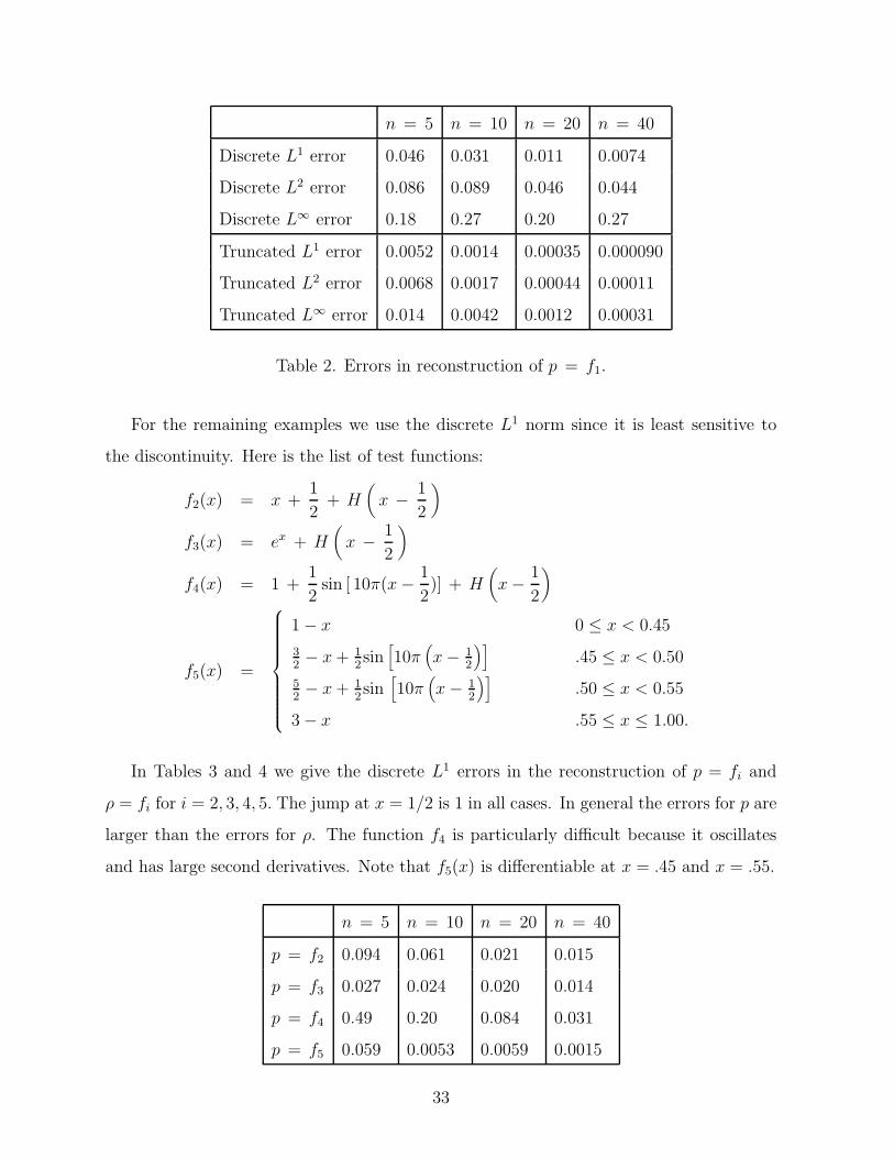
In Tables 3 and 4 we give the discrete L1 errors in the reconstruction of p = fi and

ρ = fi for i = 2, 3, 4, 5. The jump at x = 1/2 is 1 in all cases. In general the errors for p are

larger than the errors for ρ. The function f4 is particularly difficult because it oscillates

and has large second derivatives. Note that f5(x) is differentiable at x = .45 and x = .55.

n = 5 n = 10 n = 20 n = 40

p = f2 0.094 0.061 0.021 0.015

p = f3 0.027 0.024 0.020 0.014

p = f4 0.49 0.20 0.084 0.031

p = f5 0.059 0.0053 0.0059 0.0015

33

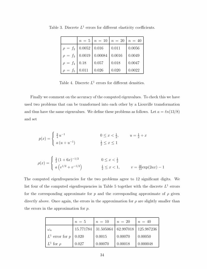
Table 3. Discrete L1 errors for different elasticity coefficients.

n = 5 n = 10 n = 20 n = 40

ρ = f2 0.0052 0.016 0.011 0.0056

ρ = f3 0.0019 0.00084 0.0016 0.0049

ρ = f4 0.18 0.057 0.018 0.0047

ρ = f5 0.011 0.026 0.020 0.0022

Table 4. Discrete L1 errors for different densities.

Finally we comment on the accuracy of the computed eigenvalues. To check this we have

used two problems that can be transformed into each other by a Liouville transformation

and thus have the same eigenvalues. We define these problems as follows. Let a = `n(13/8)

and set

p(x) =

34u−1 0 ≤ x < 1

2, u = 1

2+ x

a (u + u−1) 12≤ x ≤ 1

ρ(x) =

32(1 + 6x)−1/2 0 ≤ x < 1

2

a(

v1/2 + v−1/2)

12≤ x < 1, v = 16

13exp(2ax) − 1

The computed eigenfrequencies for the two problems agree to 12 significant digits. We

list four of the computed eigenfrequencies in Table 5 together with the discrete L1 errors

for the corresponding approximate for p and the corresponding approximate of ρ given

directly above. Once again, the errors in the approximation for ρ are slightly smaller than

the errors in the approximation for p.

n = 5 n = 10 n = 20 n = 40

ωn 15.771784 31.505064 62.997018 125.987236

L1 error for p 0.020 0.0015 0.00070 0.00050

L1 for ρ 0.027 0.00070 0.00018 0.000048

34

Table 5. Inverse nodal problems with same eigenvalues.

Acknowledgment

The authors thank L.E. Andersson, R.L. Anderssen and E.T. Trubowitz for useful dis-

cussions. The research of J.R. McLaughlin was partially supported by NSF grants VPW-

8902067, DMS-9401700 and ONR grants NOOO14-91J-1166, N)))14-96-1-0349. The re-

search of O.H. Hald was partially supported by NSF grant DMS-9503482.

35

References

[A1] L. Andersson, Inverse Eigenvalue Problems with Discontinuous Coefficients, In-

verse Problems 4 (1988), pp. 353-397.

[A2] L. Andersson, Inverse Problems for a Sturm-Liouville Equation in Impedance

Form, Inverse Problems 4 (1988), pp. 929-971.

[AT] F.V. Atkinson, Discrete and Continuous Boundary Problems, Academic Press,

1964.

[Be] J.G. Berryman, Variational structure of inverse problems in wave propagation

and vibration, Inverse Problems in Wave Propagation, Springer-Verlag, New

York, 1997, pp. 13-44.

[B] G. Borg, Eine Umkehrung der Sturm-Liouvilleschen Eigenwertaufgabe, Acta

Math. 78 (1946), pp. 1-96.

[BS] P.J. Browne and B.D. Sleeman, Inverse nodal problems for Sturm-Liouville equa-

tions with eigenparameter dependent boundary conditions, Inverse Problems 12

(1996), pp. 377-381.

[C1] R. Carlson, An Inverse Spectral Problem for Sturm-Liouville Operators with

Discontinuous Coefficients, Proc. Amer. Math. Soc. 120 (1994), pp. 475-484.

[C2] R. Carlson, R. Threadgill, and C. Shubin, Sturm-Liouville Eigenvalue Problems

with Finitely Many Singularities, JMAA 204 (1996), pp. 74-101.

[CMcL] C. Coleman and J. McLaughlin, Solution of the Inverse Spectral Problem for

an Impedance with Integrable Derivative, Parts I and II, CPAM 46 (1993), pp.

145-212.

[GL] I. Gel’fand and B. Levitan, On the determination of a differential equation from

its spectral function, Amer. Math. Soc. Transl. 1 (1955), pp. 253-304. Russian:

Izv.Akad.Nauk SSSR 5 (1951), pp. 309-360.

36

[H] O. Hald, Discontinuous Inverse Eigenvalue Problems, CPAM 37 (1984), pp. 539-

577.

[HMcL1] O. Hald and J. McLaughlin, Inverse Problems Using Nodal Position Data -

Uniqueness Results, Algorithms, and Bounds, Proceedings of the Centre for

Mathematical Analysis, Special Program in Inverse Problems, eds. R.S. Ander-

ssen and G.N. Newsam, 17 (1988), pp. 32 - 58.

[HMcL2] O. Hald and J. McLaughlin, Solutions of Inverse Nodal Problems, Inverse Prob-

lems 5 (1988), pp. 307-347.

[HMcL3] O. Hald and J. McLaughlin, Examples of Inverse Nodal Problems, Inverse Meth-

ods in Action, ed. P.C. Sabatier, Springer, 1990, pp. 147-151.

[Ho] H. Hochstadt, Asymptotic Estimates for the Sturm-Liouville Spectrum, CPAM

14 (1961), pp.749-762.

[I] E. Ince, Ordinary Differential Equations, Dover Publications, New York, 1956.

[IT] E. Isaacson and E. Trubowitz, The Inverse Sturm-Liouville Problem, I, CPAM

37 (1983), pp. 767-783.

[L] B. Levitan, Inverse Sturm-Liouville Problems, VNU Science Press, Utrecht, The

Netherlands, 1987.

[M] V. Marchenko, Sturm-Liouville Operators and Applications, Birkhauser, Basel,

1986.

[MAL] A. McNabb, R.S. Anderssen, E.R. Lapwood, Asymptotic Behavior of the Eigen-

values of a Sturm-Liouville System with Discontinuous Coefficients, JMAA 54

(1976), pp. 741-751.

[McL] J. McLaughlin, Inverse Spectral Theory Using Nodal Points as Data - A Unique-

ness Result, J. Diff. Eq. 73 (1988), pp. 354-362.

[RN] F. Riesz, B. Nagy, Functional Analysis Ungar, New York, 1955.

37

[S] C.L. Shen, On the nodal sets of the eigenfunctions of the string equations, SIAM.

J. Math. Anal. 19 (1988), pp. 1419-1424.

[ST] C.L. Shen and T-M. Tsai, On uniform approximation of the density function of

a string equation using eigenvalues and nodal points and some related inverse

nodal problems, Inverse Problems 11 (1995), pp. 1113-1123.

[W] H. H. Weinberger, Variational Methods for Eigenvalue Approximation, SIAM,

Philadelphia, 1974.

[Wi] C. Willis, Inverse Sturm Liouville Problems with Two Discontinuities, Inverse

Problems 1 (1985), pp. 263-289.

[Z] A. Zygmund, Trigonometric Series, Vol. 1, University Press, New York, 1959.

Appendix A

In this appendix we construct continuous, increasing functions Gp(x), p = 1, 2, ... and G(x)

on 0 ≤ x ≤ 1 satisfying

limp→∞

‖ Gp − G ‖∞= 0.

Each Gp will be piecewise continuously differentiable and have total variation, V (Gp) = 1;

G is in the class of Cantor functions with V (G) = 1. In addition, we establish a set of

positive integers nq with the properties

limq→∞

∫ 1

0sin (2πnqx) dG = −1, and

∫ x

0sin (2πnqx) dG ≤ 0, 0 ≤ x ≤ 1. (A.1)

Our goal is to use this result in Appendix B to show that the bound in Theorem 1 is best

possible when p(x) and ρ(x) are continuous and of bounded variation.

Our construction is explicit. Similar results, using the concept of N set instead of explicit

construction, can be found in Zygmund, [Z], for Fourier cosine coefficients. Here we use an

explicit construction as it makes our application in Appendix B easier.

38

To construct the example, let

ξ1 =4

9, ξk =

1

9kk = 2, 3, ...,

ηk =1

4− 1

2ξk, k = 1, 2, ...,

R1 = η1, Rp = η1 +p∑

k=2

ηk

k−1∏

j=1

ξj =1

4− 1

4

p−1∑

k=1

k∏

j=1

ξj −1

2

p∏

j=1

ξj, p = 2, 3, ...

Let `p0 = 0, `p

2p+1 = 1 and let `p1 < `p

2 < ... < `p2p be the ordered elements in

Lp =

Rp +1

2

ε1 + ξ1ε2 + ... + εp

p−1∏

k=1

ξk

εj = 0, 1, j = 1, 2, ..., p

, p = 2, ...

where we note that `pj + 2p−1 = 1

2+ `p

j , j = 1, ..., 2p−1. Now define

Fp =

0 , `p0 ≤ x ≤ `p

1,

j

2p, `p

j +∏p

k=1 ξk ≤ x ≤ `pj+1 , j = 1, ...2p,

(x − `pj )

2p∏p

k=1 ξk+

j − 1

2p, `p

j ≤ x ≤ `pj +

∏pk=1 ξk, j = 1, ..., 2p.

Using Fp we construct

Gp =

1 − Fp 0 ≤ x ≤ 12

Fp12

< x ≤ 1(A.2)

and note that Gp is continuous at x = 12

with Gp(12) = 1

2and that Gp(x) = Gp(1 − x).

Further V (Gp) = 1, p = 1, 2, ... Let

G(x) = limp→∞

Gp. (A.3)

Clearly, V (G) = 1. Further for each positive integer, q, let nq = 9q(q+1)/2. Then we can

establish

Theorem A:

−∫ x

0dG ≤

∫ x

0sin(2π nqx)dG ≤ −

(

1 − 8π2

92q+2

)

∫ x

0dG,

lim supn→∞

∫ 1

0sin(2πnx)dG = −1.

39

Proof of Theorem A: Set p = q +1 and let `q+1j , j = 1, 2, ..., 2q+1 be the collection of points

in Lq+1. Then the function G is decreasing on each of the subintervals

`q+1j < x < `q+1

j +q+1∏

k=1

ξk

2q

j=1

and increasing on

`q+1j < x < `q+1

j +q+1∏

k=1

ξk

2q+1

j=2q+1

.

Let

Jq =2q+1⋃

j=1

`q+1j , `q+1

j +q+1∏

k=1

ξk

.

The complement of Jq in [0, 1] is a finite collection of closed disjoint intervals. On each of

these intervals the function G is constant.

Hence∫ 1

0sin(2πnqx)dG =

2q+1∑

j=1

∫ `q+1j +

∏q+1

k=1ξk

`q+1j

sin(2πnqx)dG.

The goal is to obtain a bound on the integrals on the right side of the above inequality.

Let an arbitrary x in the interval

`q+1j < x < `q+1

j +q+1∏

k=1

ξk , j = 1, 2, ..., 2q+1

be represented by

x = `q+1j + α

q+1∏

k=1

ξk , 0 < α < 1.

Since∏q+1

k=1 ξk = 4/9q(q+1)/2, we have

2πnqx = +π

2+ 2π(nq)

(α − 1

2)

q+1∏

k=1

ξk +1

2ε1

+ 2π × (integer)

=π

2+ πε1 × (odd integer) +

4π(2α − 1)

9q+1

+ 2π × (integer).

40

Now | (2α − 1) |≤ 1. Hence for the case 0 < `q+1j < 1

2(ε1 = 0) we obtain

(

1 − 8π2

92q+2

)

≤ sin(2πnqx) ≤ 1.

Similarly, for 12

< `q+1j < 1(ε1 = 1)

−1 ≤ sin(2πnqx) ≤ −(

1 − 8π2

92q+2

)

.

Hence,

−∫ x

0dG ≤

∫ x

0sin(2πnqx)dG ≤ −

(

1 − 8π2

92q+2

)

∫ x

0dG.

The statement in the theorem follows. •

Appendix B

In this appendix we show that for p, ρ continuous and in BV [0, 1] the bound in Theorem 1

is best possible. We do this by considering the specific example where p = ρ = a(x); that

is

(aux)x + ω2au = 0, 0 ≤ x ≤ 1, (B.1)

u(0) = u(1) = 0 (B.2)

We will use the example of Appendix A to exhibit a sequence of continuous functions

aq ε BV [0, 1] satisfying

limq→∞

∣

∣

∣

∣

| ωnq − nqπ | −1

2V (`naq)

∣

∣

∣

∣

= 0.

where (ωnq)2 is the nqth eigenvalue of (B.1),(B.2) with a replaced by aq.

To begin we prove the following technical lemma.

Lemma B.1: Let G(φ) and nq, q = 1, 2, ... be as defined in Appendix A. Define

ωnq = nqπ − 1

2

∫ 1

0sin(2nqπφ)dG(φ). (B.3)

41

Then the integral equation

φ(x) =1

nqπ

{

ωnq x +1

2

∫ φ

0sin(2nqπφ)dG(φ)

}

(B.4)

has a strictly increasing solution φq(x) satisfying φq(0) = 0, φq(1) = 1.

Proof of Lemma B.1: Let

x(φ) =1

ωnq

[

nqπφ − 1

2

∫ φ

0sin(2nqπφ)dG(φ)

]

.

The function x(φ) is a continuous, strictly increasing function of φ with piecewise con-

tinuous derivative satisfying x(0) = 0, x(1) = 1. The inverse, φ(x), of x(φ) satisfies (B.4)

together with φ(0) = 0, φ(1) = 1. Label φ(x) as φq(x) and the lemma is proved. •

Having established Lemma B.1 we can immediately construct a sequence of continuous

functions a = aq(x) having (ωnq)2 as their nqth eigenvalues, q = 1, 2, ...

Lemma B.2: Let

aq(x) = exp [G(φq(x))] . (B.5)

Then the nqth eigenvalue for the eigenvalue problem

(aqux)x + ω2aq u = 0 , 0 ≤ x ≤ 1, (B.6)

u(0) = u(1) = 0

is (ωnq)2, defined in (B.3).

Proof of Lemma B.2: Construct the Prufer transformation (4) for the eigenvalue problem

(B.6). The integral equation for θ becomes

θ(x) = ωx +1

2

∫ x

0sin 2θ(x)dG(φq(x)).

Letting θ = nqπφq and ω = ωnq , then the lemma follows from (B.4). •

We can now quickly prove the desired theorem, that is, that for continuous functions

of bounded variation, p = q = a(x), the bound in Theorem 1 is best possible.

42

Theorem B: The nqth eigenvalue,(ωnq)2, for

(aqux)x + ω2aqu = 0, 0 ≤ x ≤ 1

u(0) = u(1) = 0,

q = 1, 2, .... satisfies

| ωnq(aq) − nqπ | −1

2V (`naq) ≤ 4π2

92q+2

implying

limq→∞

∣

∣

∣

∣

| ωnq − nqπ | −1

2V (`naq)

∣

∣

∣

∣

= 0.

Proof of Theorem B: Observe that

| ωnq − nqπ | −1

2V (`naq) = −1

2

∫ 1

0sin(2nqπφ)dG(φ) − 1

2V (`naq)

and that, from Lemma A.1,

− 4π2

92q+2≤ −1

2

∫ 1

0sin(2nqπφ)dG(φ) − 1

2V (`naq) ≤ 0.

The statement of the theorem follows. •

Remark: Using the same function, G, we can also construct continuous functions of

bounded variation pq(x) and ρq(x) for the eigenvalue problems

(pqux)x + ω2u = 0, 0 ≤ x ≤ 1,

u(0) = u(1) = 0,

or

uxx + ω2ρq(x) u = 0, 0 ≤ x ≤ 1,

u(0) = u(1) = 0,

respectively, to show that for these cases as well the bound in Theorem 1 is best possible.

43

Appendix C

In this appendix we establish Theorem 4 of Section 2. Without loss of generality we

consider

uxx + ω2ρu = 0, 0 ≤ x ≤ L, (B.7)

u(0) = u(L) = 0 (B.8)

where, with 0 = z0 < z1 < z2 < ... < zk+1 = L, we define

ρ(z) = b2i > 0, zi−1 ≤ z < zi, i = 1, ..., k + 1

ρ(L) = b2k+1.

Let ai = bi+1/bi. We first establish the following lemma.

Lemma C: Suppose {bi(zi − zi−1)}k+1i=1 is a rationally independent set. Then given ε > 0

and η ε [−1, 1] there exists an eigenvalue (ωn)2 for (B.7), (B.8) satisfying

ωn

∫ L

0

√ρ dx − nπ − η

k∑

i=1

arcsin

(

| ai − 1 |ai + 1

)

< ε, (B.9)

where arcsin refers to the principal value.

Proof of Lemma C: To obtain our result we return to the Prufer transformation and use

equation (5) for θ in each interval zi−1 < x < zi, i = 1, ..., k + 1. We require θ(0, ω) = 0

and that θ is continuous as a function of x everywhere in [0, L] except at each x = zi, i =

1, ...k. Letting θ−i = limx→z−iθ(x, ω) and θ+

i = limx→z+iθ(x, ω) the jump condition at each

x = zi, i = 1, ..., k is determined by (6), (7) with θ+i and θ−i chosen to be in the same

quadrant i = 1, ..., k. For each ω this yields

θx(x, ω) = ω bi, zi−1 < x < zi, i = 1, ..., k + 1, (B.10)

θ(0, ω) = 0, (B.11)

with

aitanθ−i = tanθ+i , i = 1, 2, ..., k. (B.12)

44

Further, ω is an eigenvalue provided that θ(L, ω) is a positive integer multiple of π.

We divide the proof into three cases: either η > 0, η < 0 or η = 0, and without loss

assume ai 6= 1, i = 1, ..., k. Suppose first that η > 0. Our immediate goal is to find a

real number ω that will satisfy inequality (C.3), with ωn replaced by ω, and that we will

ultimately show is close to ωn. We proceed as follows. Select δ1, ..., δk to satisfy

arctan(aiδi) − arctan(δi) = η arcsin

(

| ai − 1 |ai + 1

)

,

where arctan refers to the principal value. For each i there are two solutions of this

equation. We choose the solution closest to the origin. Now apply Kronecker’s Theorem

from number theory, see [HW, p.380], to find ω > 3π/[2 mini=1,2,...k+1(bi(zi − zi−1))] and

integers p1, ..., pk+1 satisfying

ωb1z1 − p1π + arctan(δ1) = ε1, (B.13)

ωbi(zi − zi−1) − piπ + arctan(δi) − arctan(ai−1δi−1) = εi, i = 2, ..., k, (B.14)

ωbk+1(L − zk) − pk+1π − arctan(akδk) = εk+1, (B.15)

where| εi |< ε2, i = 1, ..., k. Adding all of the above equations and letting n =∑k+1

i=1 pi we

obtain

ω∫ L

0

√ρ dx − nπ − η

k∑

i=1

arcsin

(

| ai − 1 |ai + 1

)

=k+1∑

i=1

εi < (k + 1)ε2

It remains to establish that the nth eigenvalue ωn is sufficiently close to ω.

Letting ε = ε/(2∫ L0

√ρ dx) we can show that such an eigenvalue exists if we can show

that the expressions

θ(L, ω + ε) − nπ and θ(L, ω − ε) − nπ

have opposite sign. To do this we proceed sequentially and choose ε sufficiently small when

needed. Replace ω in (B.10)-(B.11) by ω ± ε and define positive constants

Ci =i∑

j=1

bj(zj − zj−1)i∏

`=j

a`(1 + δ2` )

(1 + a2`δ

2` )

, i = 1, 2, ...k.

Using (B.10), (B.11) and (B.13) and after making a Taylor expansion we obtain

θ−1 = (ω ± ε)b1z1 = p1π − arctan(δ1) ± εb1z1 + 0(ε2),

arctan(a1 tan θ−1 ) = − arctan(a1δ1) ± C1ε + 0(ε2)

45

implying, since (B.12) is satisfied with θ−1 and θ+1 in the same quadrant, that

θ+1 = p1π − arctan(a1δ1) ± C1ε + 0(ε2). (B.16)

Similarly using (B.10), (B.14) and (B.16) we obtain

θ−2 = + θ+1 (ω ± ε)b2(z2 − z1)

= (p1 + p2)π − arctan(δ2) ± (C1 + b2(z2 − z1))ε + 0(ε2),

arctan(a2 tan θ−2 ) = − arctan(a2δ2) ± C2ε + 0(ε2).

Since θ−2 and θ+2 are in the same quadrant, it follows from (B.12) that

θ+2 = (p1 + p2)π − arctan(a2δ2) ± C2ε + 0(ε2)

...

θ+k = (p1 + ... + pk)π − arctan(akδk) ± Ckε + 0(ε2).

Now calculate θ(L, ω ± ε) = θ+k + bk+1(L − zk) using (B.15).

θ(L, ω ± ε) = (p1 + ... + pk) π − arctan(akδk) ± Ckε + 0(ε2)

+ pk+1π + arctan(akδk) ± ε bk+1(L − zk)

= nπ ± ε[bk+1(L − zk) + Ck] + 0(ε2)

implying that, for sufficiently small ε, θ(L, ω + ε)− nπ and θ(L, ω − ε)− nπ have opposite

sign. Hence the eigenvalue ωn is in the interval (ω − ε, ω + ε).

The cases η < 0 and η = 0 are handled similarly. The lemma is proved. •

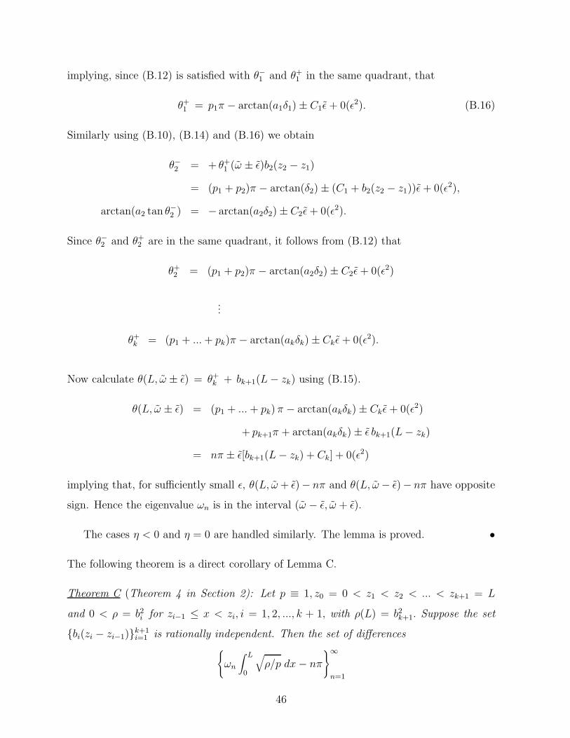
The following theorem is a direct corollary of Lemma C.

Theorem C (Theorem 4 in Section 2): Let p ≡ 1, z0 = 0 < z1 < z2 < ... < zk+1 = L

and 0 < ρ = b2i for zi−1 ≤ x < zi, i = 1, 2, ..., k + 1, with ρ(L) = b2

k+1. Suppose the set

{bi(zi − zi−1)}k+1i=1 is rationally independent. Then the set of differences

{

ωn

∫ L

0

√

ρ/p dx − nπ

}∞

n=1

46

is dense in the interval [−A0, A0] where

A0 =k∑

i=1

arcsin

(

| ai − 1 |ai + 1

)

.

47