Inverse modeling of interbed storage parameters using land ... · PDF fileInverse modeling of interbed storage parameters using land subsidence observations, Antelope Valley, California

Inverse modeling of interbed storage parameters using land

subsidence observations, Antelope Valley, California

Jorn Hoffmann

Department of Geophysics, Stanford University, Stanford, California, USA

Devin L. Galloway

U.S. Geological Survey, Sacramento, California, USA

Howard A. Zebker

Department of Geophysics, Stanford University, Stanford, California, USA

Received 14 February 2002; revised 25 July 2002; accepted 25 July 2002; published 13 February 2003.

[1] We use land-subsidence observations from repeatedly surveyed benchmarks andinterferometric synthetic aperture radar (InSAR) in Antelope Valley, California, toestimate spatially varying compaction time constants, t, and inelastic specific skeletalstorage coefficients, Skv*, in a previously calibrated regional groundwater flow andsubsidence model. The observed subsidence patterns reflect both the spatial distribution ofhead declines and the spatially variable inelastic skeletal storage coefficient. Using thenonlinear parameter estimation program UCODE we estimate compaction time constantsbetween 3.8 and 285 years. The Skv* values are estimated by linear estimation and rangefrom 0 to almost 0.09. We find that subsidence observations over long time periods arenecessary to constrain estimates of the large compaction time constants in AntelopeValley. The InSAR data used in this study cover only a three-year period, limiting theirusefulness in constraining these time constants. This problem will be alleviated as moreSAR data become available in the future or where time constants are small. Byincorporating the resulting parameter estimates in the previously calibrated regionalmodel of groundwater flow and land subsidence we can significantly improve theagreement between simulated and observed land subsidence both in terms of magnitudeand spatial extent. The sum of weighted squared subsidence residuals, a commonmeasure of model fit, was reduced by 73% with respect to the original model. However,the ability of the model to adequately reproduce the subsidence observed over only afew years is impaired by the fact that the simulated hydraulic heads over small timeperiods are often not representative of the actual aquifer hydraulic heads. Errors in thesimulated hydraulic aquifer heads constitute the primary limitation of the approachpresented here. INDEX TERMS: 1829 Hydrology: Groundwater hydrology; 1894 Hydrology:

Instruments and techniques; 8020 Structural Geology: Mechanics; KEYWORDS: subsidence, InSAR, storage,

compaction, estimation

Citation: Hoffmann, J., D. L. Galloway, and H. A. Zebker, Inverse modeling of interbed storage parameters using land subsidence

observations, Antelope Valley, California, Water Resour. Res., 39(2), 1031, doi:10.1029/2001WR001252, 2003.

1. Introduction

[2] Land subsidence caused by the compaction of sus-ceptible aquifer systems has been related to groundwaterlevel declines accompanying the development of ground-water resources [e.g., Tolman and Poland, 1940; Riley,1969; Poland et al., 1975; Bell and Price, 1991; Holzer,1984, 1979; Ikehara and Phillips, 1994; Galloway et al.,1998a]. A large number of case studies have documentedthe global scale of the problem [e.g., Galloway et al., 1999;Johnson, 1991; Barends et al., 1995]. While no compre-hensive assessment of the costs related to land subsidence

has been made, the annual costs from flooding and struc-tural damage caused by land subsidence probably exceeds$125 million [National Research Council, 1991]. Gallowayet al. [1999] argue convincingly that the actual cost wouldbe much higher if all related effects were accounted for. Theobstacles Galloway et al. [1999] cite in realistically assess-ing these costs include difficulties in mapping the affectedareas and establishing cause-and-effect relations. The appli-cation of space-borne InSAR techniques to detect andmonitor ongoing land subsidence [Galloway et al., 1998a;Amelung et al., 1999] has greatly enhanced our ability toobserve and quantify land subsidence at a regional scale.Further, Hoffmann et al. [2001] have used time seriesInSAR observations and water levels measured in wells toestimate spatially varying aquifer system elastic storage

Copyright 2003 by the American Geophysical Union.0043-1397/03/2001WR001252

SBH 5 - 1

WATER RESOURCES RESEARCH, VOL. 39, NO. 2, 1031, doi:10.1029/2001WR001252, 2003

coefficients. Lu and Danskin [2001] and Bawden et al.[2001] have employed InSAR to help define the structure ofgroundwater basins.[3] A number of studies have used historical subsidence

data obtained from borehole extensometers [e.g., Helm,1975, 1976; Hanson and Benedict, 1994; Sneed and Gallo-way, 2000] and repeat surveys of benchmarks [e.g., Wil-liamson et al., 1989; Hanson and Benedict, 1994; Leightonand Phillips, 2003; Nishikawa et al., 2001] in the calibra-tion of groundwater flow and subsidence models. No workto date has attempted to use the available land subsidencedata from InSAR to constrain models of regional ground-water flow and aquifer-system compaction. The mainobjective of this paper is to present an approach to usesubsidence observations from benchmark leveling andInSAR in conjunction with aquifer heads simulated in apreviously calibrated regional groundwater flow model toestimate spatially variable inelastic skeletal storage coeffi-cients and compaction time constants of compressibleinterbeds.

2. Antelope Valley Aquifer System

[4] Antelope Valley is a topographically closed, triangu-lar basin located about 80 km northeast of Los Angeles,California (Figure 1). The sedimentary basin is bounded bythe Tehachapi mountains in the northwest and the SanGabriel mountains in the southwest. The eastern boundaryis less clearly defined by lower hills. The basin has beenfilled to depths of more than two kilometers with fluvial andlacustrine sediments forming the aquifer system that hasprovided much of the water supply for agriculture and the

growing communities in Antelope Valley since the late1800s. The valley floor has very little topographic reliefand is dominated by two large playas, Rosamond Lake andRogers Lake.[5] The first extensive investigation into the water

resources of Antelope Valley was undertaken by Johnson[1911], who judged the water resources to be sufficient andaccessible enough to merit agricultural development ofmuch of the valley. Artesian conditions existed over largeparts of the central Antelope Valley. Development of thegroundwater resource during the early part of the twentiethcentury led to groundwater withdrawals vastly exceedingthe natural recharge, causing large scale drawdowns of thehydraulic heads. Annual pumpage peaked at 400 hm3

(300,000 acre-ft) in 1950 [Snyder, 1955]. During thesecond half of the twentieth century the declining ground-water levels made pumping increasingly uneconomical,resulting in a decline of both irrigated acreage and annualpumpage [Durbin, 1978]. The trend of decreasing pumpingrates was discontinued in the 1990s, when groundwateruse shifted from primarily agricultural to municipal-indus-trial to support the rapidly growing communities in thevalley, primarily Lancaster and Palmdale [Galloway et al.,1998b].[6] The groundwater basin has been conceptually sub-

divided into 12 subbasins [Bloyd, 1967]. The Lancastersubbasin (Figure 1) is the largest and most developed ofthese. All subsidence simulated in this study occurs withinthe Lancaster subbasin. The aquifer system in the Lancastersubbasin has been conceptualized using two or three aqui-fers. Earlier reports identified two aquifers, a principal and adeep aquifer [e.g., Bloyd, 1967; Durbin, 1978], which are

Figure 1. Antelope Valley, California. The area shown is the full extent of the MODFLOW grid. Theblue frame encloses the area shown in Figures 3, 6, 7 and 8. The radar amplitude image covers the areawithin the model region that is covered by the interferograms. Major roads (red) and the playas are shownfor reference. The thick black lines delineate groundwater subbasins conceptualized by Bloyd [1967]. TheLancaster subbasin is the largest and most important subbasin, both in terms of groundwater pumping andsubsidence. The black circle indicates the location where the data shown in Figure 2 was obtained and thegreen symbols (A–D) indicate locations for the curves in Figure 9. The yellow lines delineate theparameter zones used for inversion of the time constants.

SBH 5 - 2 HOFFMANN ET AL.: INVERSE MODELING OF INTERBED STORAGE

vertically separated by a laterally extensive lacustrine unit,where this is present. The lacustrine unit extends fromRogers Lake, where it is exposed at the land surface, downdip to the south west. Near the southern end of the valleythe lacustrine unit is overlain by over 200 m of alluvium[Sneed and Galloway, 2000]. Referring to more recent data,Sneed and Galloway [2000], Nishikawa et al. [2001] andLeighton and Phillips [2003] use a conceptual model withthree aquifers termed the upper, middle and lower aquifer.According to Durbin [1978], most of the water is producedfrom the principal (unconfined) aquifer, while Sneed andGalloway [2000], Nishikawa et al. [2001], and Leightonand Phillips [2003] consider the upper aquifer as generallyunproductive and the middle (confined) aquifer to be themost productive. Low-permeability interbeds consisting ofcompressible, unconsolidated deposits are present through-out the aquifer system.

3. Delayed Compaction

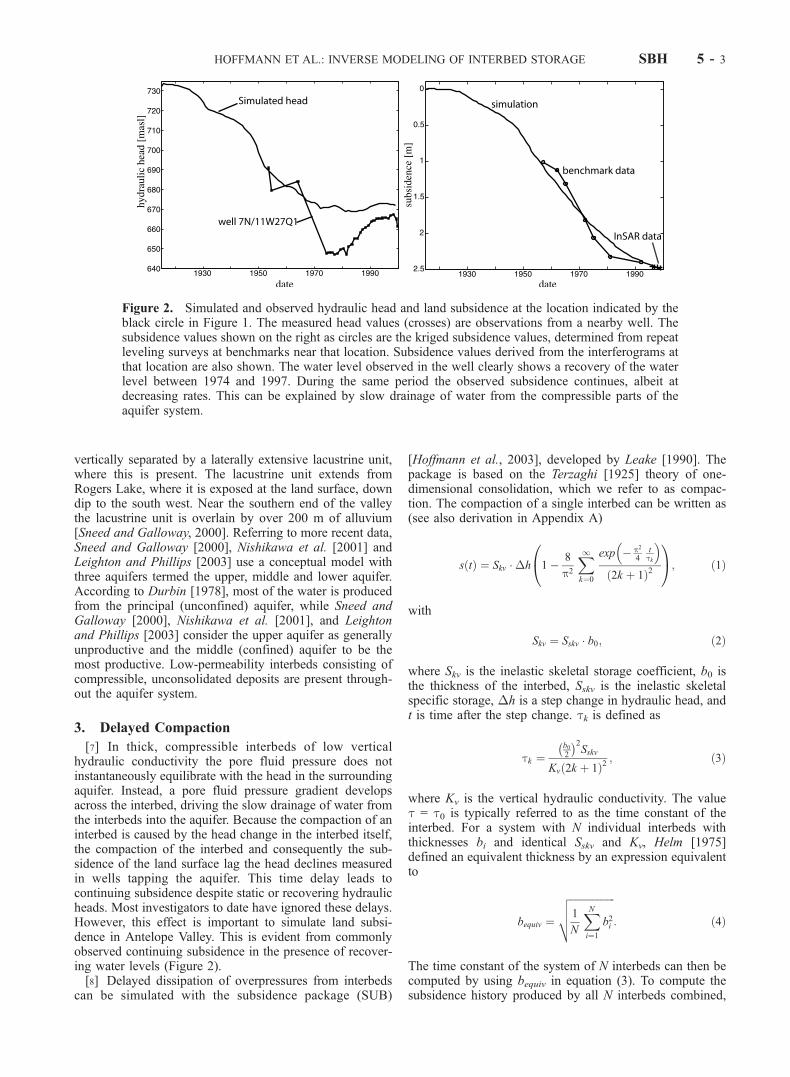
[7] In thick, compressible interbeds of low verticalhydraulic conductivity the pore fluid pressure does notinstantaneously equilibrate with the head in the surroundingaquifer. Instead, a pore fluid pressure gradient developsacross the interbed, driving the slow drainage of water fromthe interbeds into the aquifer. Because the compaction of aninterbed is caused by the head change in the interbed itself,the compaction of the interbed and consequently the sub-sidence of the land surface lag the head declines measuredin wells tapping the aquifer. This time delay leads tocontinuing subsidence despite static or recovering hydraulicheads. Most investigators to date have ignored these delays.However, this effect is important to simulate land subsi-dence in Antelope Valley. This is evident from commonlyobserved continuing subsidence in the presence of recover-ing water levels (Figure 2).[8] Delayed dissipation of overpressures from interbeds

can be simulated with the subsidence package (SUB)

[Hoffmann et al., 2003], developed by Leake [1990]. Thepackage is based on the Terzaghi [1925] theory of one-dimensional consolidation, which we refer to as compac-tion. The compaction of a single interbed can be written as(see also derivation in Appendix A)

s tð Þ ¼ Skv ��h 1� 8

p2

X1k¼0

exp � p2

4ttk

� �2k þ 1ð Þ2

0@

1A; ð1Þ

with

Skv ¼ Sskv � b0; ð2Þ

where Skv is the inelastic skeletal storage coefficient, b0 isthe thickness of the interbed, Sskv is the inelastic skeletalspecific storage, �h is a step change in hydraulic head, andt is time after the step change. tk is defined as

tk ¼b02

� 2Sskv

Kv 2k þ 1ð Þ2; ð3Þ

where Kv is the vertical hydraulic conductivity. The valuet = t0 is typically referred to as the time constant of theinterbed. For a system with N individual interbeds withthicknesses bi and identical Sskv and Kv, Helm [1975]defined an equivalent thickness by an expression equivalentto

bequiv ¼

ffiffiffiffiffiffiffiffiffiffiffiffiffiffiffiffiffiffi1

N

XNi¼1

b2i

vuut : ð4Þ

The time constant of the system of N interbeds can then becomputed by using bequiv in equation (3). To compute thesubsidence history produced by all N interbeds combined,

Figure 2. Simulated and observed hydraulic head and land subsidence at the location indicated by theblack circle in Figure 1. The measured head values (crosses) are observations from a nearby well. Thesubsidence values shown on the right as circles are the kriged subsidence values, determined from repeatleveling surveys at benchmarks near that location. Subsidence values derived from the interferograms atthat location are also shown. The water level observed in the well clearly shows a recovery of the waterlevel between 1974 and 1997. During the same period the observed subsidence continues, albeit atdecreasing rates. This can be explained by slow drainage of water from the compressible parts of theaquifer system.

HOFFMANN ET AL.: INVERSE MODELING OF INTERBED STORAGE SBH 5 - 3

the value computed using equation (1) can then be multipliedby the factor

n ¼ 1

bequiv

XNi¼1

bi ¼S�kv

Sskvbequiv; ð5Þ

where Skv* denotes the cumulative inelastic skeletal storagecoefficient for all N interbeds. The second equality assumesthat Sskv is the same for all interbeds. Note that equation (5)does not require the knowledge of all bi, but only of theirsum. The factor n can be used to parameterize the distributionof the total interbed storage into individual interbeds. Bydefinition n is always greater than or equal to one.

4. Approach

[9] We modified a previously calibrated regional ground-water flow and aquifer-system compaction model of Ante-lope Valley [Leighton and Phillips, 2003] to improve theagreement between the simulated aggregate compaction(land subsidence) and the observations at benchmarksand in InSAR-derived displacement maps. The Leightonand Phillips [2003] model uses MODFLOW [McDonaldand Harbaugh, 1988] with the interbed storage package(IBS1) [Leake and Prudic, 1991] to simulate subsidence. Itis based on a regular model grid with 1 by 1 mile gridcells, extending 60 miles (97 km) from west to east and 43miles (69 km) from south to north. The model area isshown in Figure 1. Three model layers are used to simulategroundwater flow. All model boundaries are represented asno-flow boundaries. Small amounts of run-off entering theaquifer system along the foot of the mountains in the south,west and northwest represent the only natural recharge tothe system. Evapotranspiration and groundwater pumpingare the only simulated mechanisms for water to leave thesystem. The aquifer system is stressed by hydraulic headchanges caused by pumping from the upper two modellayers. Estimates of annual pumpage used in the modelwere based on measured values for municipal/industrialwater use. For agricultural water use estimates were basedon a water budget analysis for the types of crops that werecultivated and published in annual crop reports. Aquifer-system compaction caused by compaction of compressiblesediments interbedded in the aquifer system is simulated inthe upper two model layers. Our modifications to thisoriginal model were limited to the representation ofinterbed storage. We accounted for the time delays dis-cussed in the previous section by using the SUB packageto simulate compaction in the interbeds and resultingsubsidence. The IBS1 package used by Leighton andPhillips [2003] assumes the instantaneous equilibration ofthe heads in the interbeds with the heads in the surroundingaquifers. This assumption is valid for interbeds with veryshort time constants, such as thin interbeds. The SUBpackage used in this study employs a numerical techniqueto compute the head profile across the interbeds at everyMODFLOW iteration and the slow accrual of compactionas the residual pore fluid overpressures are dissipated.

4.1. Subsidence Data

[10] We used two kinds of subsidence data in this study,leveling observations from repeated benchmark surveys and

InSAR-derived subsidence maps. Several benchmark level-ing surveys have been conducted in Antelope Valley bydifferent agencies and according to various standards.Ikehara and Phillips [1994] compiled a comprehensive dataset of subsidence values from various surveys. Their table 9contains subsidence magnitudes for over 250 benchmarksduring the six time periods, 1957–62, 1962–65, 1965–72,1972–75, 1975–81, and 1981–92. Furthermore, they usedthe data acquired in these campaigns and an earlier sub-sidence map by Mankey [1963] to estimate land subsidencebetween 1930–92. In order to constrain the parameterestimates more easily spatially and to simplify the relativeweighting of the benchmark and InSAR observations in theinversion, we interpolated these subsidence values at loca-tions away from the benchmark locations using a kriginginterpolator. We employed ordinary kriging [Deutsch andJournel, 1998] with an isotropic gaussian variogram modelthat was fit to the available subsidence data for each of thesix time periods.[11] The second kind of subsidence data used to constrain

the inversions in this study were InSAR-derived displace-ment maps. We formed 22 interferograms from 17 SARscenes acquired by the European Remote-Sensing satellite 2(ERS-2) between January 26, 1996 and May 1, 1999(Figure 3). All interferograms were formed using preciseorbit information [Scharroo and Visser, 1998] and correctedfor topography using a digital elevation model (two-passmethod [Massonnet et al., 1993]). Phase unwrapping wasperformed using a minimum-cost network-flow algorithm[Costantini, 1998]. Any residual linear phase slopes acrossthe image were removed using tie-points outside thedeforming areas. The resulting interferograms can be inter-preted in terms of vertical surface displacements, if anyhorizontal displacements and atmospheric delay differencesbetween the acquisition are assumed to be negligible.Horizontal displacements have been observed near pumpingcenters or near the boundaries of an aquifer system [Bawdenet al., 2001; Watson et al., 2002] and neglecting thesedisplacements may lead to an over- or underestimation ofthe vertical displacement where they are significant. How-ever, the steep incidence angle of the ERS-2 satellite (23�)ensures that the measurement sensitivity to horizontal dis-placements is at most about 42% of that to vertical displace-ments, depending on the direction of the horizontaldisplacement component with respect to the line of sightof the satellite. The resulting error from misinterpreting ahorizontal deformation signal as vertical displacement istherefore both small and spatially localized and is unlikelyto seriously affect our analysis. In order to assess the levelof accuracy achieved in the InSAR-derived displacementmaps, we compared them with compaction data from thetwo borehole extensometers operating in Antelope Valley(Figure 4). The agreement between the two measurements isvery good. Only at a few times do the two measurementsdiffer by more than 5 mm and often this can be traced backto an obvious artifact in the corresponding image. Seasonaldisplacements caused by seasonally fluctuating groundwaterlevels are clearly obvious in Figure 4. These seasonalobservations can be used to estimate elastic storage coef-ficients [Sneed and Galloway, 2000; Hoffmann et al., 2001].However, for this study we adopted the use of annual stressperiods used in the Leighton and Phillips [2003] model, and


thus did not consider seasonal stresses. In general, seasonalhead fluctuations only lead to recoverable, elastic displace-ments. Neglecting these fluctuations therefore does notsignificantly affect the estimation of parameters governinginelastic compaction. This assessment was verified bynumerical simulations. We combined (stacked) 13 of theimages to create 3 displacement maps approximately cover-ing the years 1996–1998, 1997–1998 and 1998 (Figure 3).This approach removes the seasonal signal from the obser-

vations (Figure 4) and decreases the level of (temporallynoncoherent) atmospheric noise.

4.2. Parameterization

[12] According to equations (1) and (2) the compaction ina system of interbeds due to a unit step decrease inhydraulic head depends on the time constant t, the inelasticskeletal specific storage, Sskv, and the thickness of thecompacting interbeds. The time constant only affects the

Figure 4. Comparison of compaction measured by the Lancaster and Holly extensometers and theInSAR-derived subsidence. Each cross represents one SAR acquisition. The diamonds show thesubsidence measured in the composite images used for the inversion. Water level observations from wellscolocated with the extensometers are shown for reference (labeled with well name). The surfacedisplacement measurements at the Lancaster site agree well within the expected accuracies, suggestingthat little compaction is occurring below the anchoring depths of the extensometers (363 m). At the Hollysite the seasonal displacement fluctuations are stronger in the InSAR-derived values, indicating elasticdisplacements below the anchoring depth of that extensometer (256 m).

Figure 3. Interferometric data and derived composite subsidence maps. The bars indicate the timesspanned by the 22 interferograms used in this study. The ERS-2 orbit numbers of the acquisitions used toform the interferograms are indicated. The interferograms underlain in color were used to create the threecomposite images shown on the right. These images were used in constraining the parameter inversion.The satellite line of sight (LOS) direction is indicated by the arrow in the subsidence maps.


timing of the compaction, but not the ultimate magnitude ofthe subsidence. The actual subsidence can be thought of as aconvolution of the compaction in equation (1) and thedrawdown history, assuming that the stress-dependence ofKv and Sskv is negligible. Although both Kv and Sskv havebeen shown to be stress-dependent for many geologicmaterials, the effect of neglecting this stress-dependence issmall for stress-changes typical for water level drawdowns indeep aquifer systems [Leake and Prudic, 1991]. Becausedifferent sets of Kv, Sskv and bequiv result in the same timeconstant (equation (3)), and hence the same subsidencehistory, these parameters cannot be resolved independentlyusing only land subsidence measurements. Similarly, theinelastic skeletal specific storage, Sskv, of the interbedscannot be separated from the interbed thickness using surfacesubsidence measurements alone. We therefore estimate thetime constant, t, and the total inelastic skeletal storagecoefficient, Skv*, which is the product of Sskv and the cumu-lative interbed thickness. The estimated value for Skv* can betranslated into an estimate of the cumulative interbed thick-ness if a value for Sskv is either assumed or available fromindependent information (equation (5)). If the verticalhydraulic conductivity, Kv, is also assumed or known, theequivalent thickness of the interbeds can be computed fromthe estimated time constants (using bequiv in equation (3)),yielding information on the distribution of the compressiblesediments into individual interbeds (equation (4)).

4.3. Zoning and Parameter Inversion

[13] Because of the spatial heterogeneity of the skeletalstorage coefficient in the aquifer system it is of interest toderive spatially varying estimates rather than average valuesfor the entire aquifer system. This is particularly importantin areas where relatively large subsidence gradients maypoint to heterogeneities. The InSAR-derived subsidencemaps can afford the spatial detail necessary to make thesespatially variable estimates. However, observations overperiods on the order of the compaction time constants arenecessary to reliably constrain these estimates. Unfortu-nately, SAR data suitable for interferometry have only beenacquired for about 10 years, and the data used in this studyonly cover about a three year period. This proved to be tooshort to constrain the large time constants in AntelopeValley. Thus the inversion of the time constants has to relyprimarily on benchmark data which cover a large part of thecentury, but do not afford the high spatial detail of theInSAR maps. To overcome this problem we defined sixparameter zones (Figure 1). The definition of these zoneswas based on a zonation in the original Leighton andPhillips [2003] model, which we modified slightly basedon spatial structure observed in the InSAR images andinitial inversion results. These parameter zones were onlyused to estimate the time constants. The inelastic skeletalstorage coefficient, Skv*, was allowed to vary at each of the282 model cells within the 6 parameter zones.[14] For a given drawdown history and time constant, the

subsidence is linearly related to the inelastic skeletalstorage coefficient (equation (1)). While this is onlyapproximately true in the presence of elastic compaction,it is a reasonable assumption for interbeds, where the ratioof Sskv to Sske (the inelastic and elastic skeletal specificstorage values) is generally large. This recognition enabled

the more efficient two-level inversion described in thefollowing paragraph. A flow diagram of the estimationapproach is shown in Figure 5.[15] After simulating the initial drawdown histories in a

MODFLOW simulation using initial estimates for Skv* and t,we used the general-purpose inversion code UCODE[Poeter and Hill, 1998] to perform a nonlinear parameterestimation of the time constants in all 6 parameter zones(shaded box in Figure 5). UCODE employs a modifiedGauss-Newton method to solve a general nonlinear regres-sion problem iteratively. Thus it minimizes the weightedsquared differences between the simulation and the con-straining observational subsidence data (described above),repeatedly running the model in the process. Every modelrun consisted of the following steps (Figure 5).1. Estimate the best Skv* value for all locations inside the

parameter zones using linear least squares and an auxiliaryprogram to compute one-dimensional subsidence for thelocal drawdown history.2. Convert these Skv* estimates and the time constants to

the input parameters required by the SUB package.

Figure 5. Flowchart for the estimation of Skv* and t. TheSkv* values are estimated in a linear estimation (step 1) andthe t values are estimated nonlinearly by UCODE. Theaquifer heads, hit(x, y, t) are updated in every UCODEiteration (it) through a new MODFLOW simulation.


3. Run the MODFLOW model to simulate groundwaterflow and land subsidence for the entire model domain.[16] Several points need to be noted regarding these steps.

Employing a linear inversion to estimate the inelasticskeletal storage coefficients (step 1) makes this step veryefficient. However, it inherently decouples the interbedcompaction from the flow system, which is affected bythe water expelled from, or taken up by, the interbeds. Thecoupled system is solved in the MODFLOW simulation. Toavoid biasing the solution we compared the drawdownhistory of the last iteration (used to compute the subsidencein step 1) to the final MODFLOW-computed drawdownhistory. As long as we observed significant differences, werepeated the estimation, using the new drawdown history.After 2 iterations the maximum difference in the drawdownswas less than 1 cm.[17] The parameters required for the SUB package are

the vertical hydraulic conductivity of the interbeds, Kv, theelastic and inelastic values of skeletal specific storage ofthe interbeds, Sske and Sskv, the equivalent thickness of thesystem of interbeds, bequiv, and the factor n, defined inequation (5). We used Kv = 1.2 � 10�5 ft/d (4.2 � 10�11 m/s),Sske = 1.7 � 10�6 ft�1 (5.6 � 10�6 m�1), and Sskv = 3.5 �10�4 ft�1 (1.1 � 10�3 m�1). These are the values foraquitards thicker than 18 ft, estimated by Sneed and Gallo-way [2000] from inverse modeling of extensometer com-paction data and hydraulic head measurements in colocatedwells at the Holly site, south of Rogers Lake. Using thesevalues the estimated time constant and inelastic skeletalstorage coefficient, Skv*, can be translated into an equivalentthickness of the interbeds and the factor n. At somelocations, this led to a value of n that was smaller than 1,meaning that with the assumed values for Sskv and Kv, asingle interbed of thickness bequiv would lead to an over-estimation of the subsidence at that location. Instead oflocally modifying Sskv or Kv we chose to decrease the timeconstant t at that location, which corresponds to a decreasein bequiv. We then repeated the linear estimation of Skv* untilthe factor n was at least 1. This prevents the time constants

from being strictly constant within the parameter zones(Figure 6a).[18] It is important in both the UCODE inversion and the

linear least squares inversion to assess the relative weightsgiven to the different subsidence observations. Both theUCODE cost function and the linear inversion weight thedata residuals according to the variance of the correspond-ing observation. It is difficult to assess measurement var-iances that adequately account for all error sources. Becauseof the high accuracy in precision leveling surveys thevariance in the benchmark data is dominated by the inter-polation and averaging over spatially varying values. Weused the spatially varying kriging variance (from the kriginginterpolation of the benchmark subsidence maps describedabove) at the center of each model cell as the measurementvariance of the benchmark values at that location. Thisaccounts for the increasing uncertainty distant from theactual benchmarks. We also enforced a minimum varianceat the level of the theoretical variance within one model gridcell (using the variogram model) to avoid unreasonablysmall variances where a benchmark was very close to thecell center.[19] For the InSAR-derived subsidence values we assume

a spatially constant variance of 50 mm2. While this is asubjective choice it addresses an attempt to include twoseparate error sources. The first is the measurement variancemostly due to atmospheric disturbances. As discussed abovethe importance of random atmospheric errors in the imagesare reduced by the stacking of several individual interfero-grams to produce the composite images. We thereforeassume a variance of 25 mm2 for this error source. Thiscorresponds to a standard deviation of 5 mm, which isapproximately the level at which atmospheric artifacts in theInSAR-derived subsidence maps would become clearlyvisible. The agreement between the compaction trendsmeasured by the extensometer instruments and the long-term subsidence values determined from the InSAR sub-sidence maps (Figure 4) supports this estimate of theachieved accuracy for the two extensometer locations. The

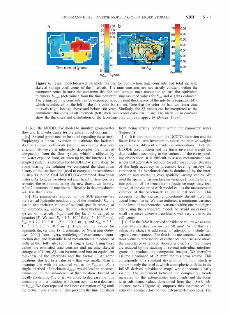
Figure 6. Final model-derived parameter values for compaction time constants and total inelasticskeletal storage coefficients of the interbeds. The time constants are not strictly constant within theparameter zones because the constraint that the total storage must amount to at least the equivalentthickness, bequiv (determined from the time constant using assumed values for Sskv and Kv) was enforced.The estimated time constants can be expressed as equivalent thicknesses of the interbeds (equation (4)),which is indicated on the left of the first color bar (in m). Note that the color bar has two linear timeintervals (right labels), above and below 100 years. Similarly, the Skv* values can be interpreted as thecumulative thickness of all interbeds (left labels on second color bar, in m). The black 20 m contoursshow the thickness and distribution of the lacustrine clay unit as mapped by Durbin [1978].


second error source is related to the variance of the actualsubsidence values within a model grid cell. Again, weassign a variance of 25 mm2 to this error source. This valueis approximately the mean experimental variance of theInSAR-derived subsidence within one grid cell. All threeInSAR-derived displacement maps share a common refer-ence year (1999) and common data acquisitions. Thiscorrelation is accounted for in the covariance matrix usedin the linear inversions for Skv* at each location.

5. Results

[20] The resulting parameter estimates for t and Skv* showsignificant spatial variability (Figure 6 and Table 1). Theestimated compaction time constants range from 20.5 yearsin zone 5 to 284.9 years in zone 2 (Table 1). Nonlinear 95%confidence intervals for the estimated time constants arealso computed by UCODE (Table 1). The estimated com-paction time constants are not strictly constant within eachparameter zone and time constants as low as 3 years occurin the final results (Figure 6a), because the time constantwas locally decreased to ensure physically reasonableresults (see previous section). Using the Sskv and Kv esti-mates from Sneed and Galloway [2000], these valuescorrespond (equation (3)) to an equivalent thicknessbetween 3.8 m and 36.4 m (Figure 6a).[21] The resulting inelastic skeletal storage coefficients,

Skv* range from zero at the boundaries of the estimationdomain to almost 0.09 in zone 2 (Figure 6b). Again usingSskv from Sneed and Galloway [2000] this translates (equa-tion (5)) to cumulative interbed thicknesses up to 77 m(Figure 6b). Another result afforded by the linear inversionsis a spatially varying estimation variance (not shown). Thisvariance reflects the spatially variable variances of theobservational data and the goodness of fit but does notinclude any uncertainties related to imprecise or unrepre-sentative drawdown histories used in the inversions.[22] The simulated subsidence agrees well with the kriged

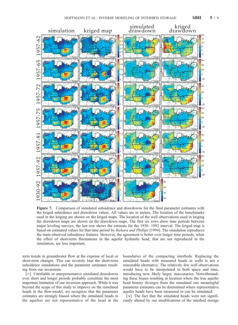
subsidence maps derived from the benchmark observations(Figure 7). Both the magnitude of the subsidence and thespatial pattern of the subsidence field are reproducedadequately. This agreement represents a significantimprovement with respect to the original Leighton andPhillips [2003] model. The total UCODE cost function,computed as the sum of the weighted squared residualsbetween subsidence data and simulation decreased by about73% with respect to that model. It is important to note thatdespite the spatial continuity suggested by the kriged sub-sidence maps (Figure 7), the data lack the spatial detailafforded by the InSAR data. Small-scale heterogeneities in

the subsidence field are not observed at the sparselydistributed benchmarks or smoothed out in the interpola-tion, biasing the estimates derived from them.[23] The agreement of the simulated subsidence with the

InSAR-derived subsidence maps (Figure 3) has alsoimproved with respect to the original model. The costfunction computed from the residuals for only these datadecreased by 30%. The residuals (simulated subsidenceminus InSAR maps) show that the simulation overestimatesthe subsidence during the time period covered by InSAR(Figure 8). This systematic disagreement can at least in partbe explained by simulated drawdowns exceeding the actualdrawdowns during this time period, as suggested by thecomparison with kriged drawdowns derived from severalwells in the area (Figure 8). As discussed in the followingsection, this should not be misinterpreted to mean thatkriged heads are more representative of true aquifer headsin general though. The good agreement between simulatedand observed subsidence is also shown for four pointlocations marked in Figure 1 (Figure 9).[24] Another important result of this study is the effect of

our modifications to the interbed storage in the model on thesimulated aquifer heads. We found that over the long term,these modifications did not significantly alter the flow fieldin the aquifers, although the simulated interbeds suppliedlarge volumes of water to the wells. Over the simulated 84years an average of 5% of the water pumped from wellsoriginated from interbeds, with peak values of 10% in someyears. Introducing delay in the interbed drainage causedlarger initial drawdowns in the aquifer after the onset ofpumping. These larger drawdowns increased the headgradient across the interbeds, causing them to drain at ahigher rate. However, within a few years the head in ourmodified model returned to the level found in the originalLeighton and Phillips [2003] model.

6. Discussion

[25] The resulting parameter estimates reflect the spatialheterogeneity of interbed storage in the aquifer system,which causes the uneven distribution of subsidence whensufficiently large and widespread drawdowns occur. It isimportant to observe that the subsidence pattern is not solelydue to the spatial distribution of drawdowns, but reflects thespatial variability of the skeletal storage coefficients of theinterbeds.[26] The simulated land subsidence for the final param-

eter estimates agrees much more closely with the observa-tions than the subsidence simulated by the original Leightonand Phillips [2003] model, as evidenced by the 73%decrease of the UCODE-computed cost function. Both themagnitude and spatial extent of the subsidence are repro-duced much better in our modified model. However, whilethe simulated subsidence captures the timing and magnitudeof the main subsidence features, some important differencesstill remain. These differences highlight the limitations ofthe approach presented here. Particularly over time periodsof only a few years, the simulation does not adequatelyreproduce the observed subsidence (Figure 7, first row, andFigures 8 and 9). This is likely caused by short-termfluctuations in hydraulic head that are not reproduced inthe flow simulation. In calibrating the regional flow modelemphasis was placed on simulating regional-scale and long-

Table 1. Time Constants and UCODE-Determined Confidence

Intervals for the Six Parameter Zonesa

Zone t, years 95% Confidence Interval

1 40.8 [38.3, 43.5]2 284.9 [207.8, 550.3]3 77.3 [73.1, 81.6]4 94.7 [91.4, 97.7]5 20.5 [10.2, 30.7]6 39.1 [29.0, 49.3]

aThe estimates in zones 2 and 5 are very poorly constrained owing to thelack of sufficient historical subsidence information in these zones.


term trends in groundwater flow at the expense of local orshort-term changes. This can severely bias the short-termsubsidence simulations and the parameter estimates result-ing from our inversions.[27] Unreliable or unrepresentative simulated drawdowns

over short and longer periods probably constitute the mostimportant limitation of our inversion approach. While it wasbeyond the scope of this study to improve on the simulatedheads in the flow-model, we recognize that the parameterestimates are strongly biased where the simulated heads inthe aquifers are not representative of the head at the

boundaries of the compacting interbeds. Replacing thesimulated heads with measured heads in wells is not areasonable alternative. The relatively few well observationswould have to be interpolated in both space and time,introducing new, likely larger, inaccuracies. Notwithstand-ing these biases resulting at location where the true aquiferhead history diverges from the simulated one meaningfulparameter estimates can be determined where representativeaquifer heads have been measured or can be simulated.[28] The fact that the simulated heads were not signifi-

cantly altered by our modifications of the interbed storage

Figure 7. Comparison of simulated subsidence and drawdowns for the final parameter estimates withthe kriged subsidence and drawdown values. All values are in meters. The location of the benchmarksused in the kriging are shown on the kriged maps. The location of the well observations used in krigingthe drawdown maps are shown on the drawdown maps. The first six rows show time periods betweenmajor leveling surveys; the last row shows the estimate for the 1930–1992 interval. The kriged map isbased on estimated values for that time period by Ikehara and Phillips [1994]. The simulation reproducesthe main observed subsidence features. However, the agreement is better over longer time periods, whenthe effect of short-term fluctuations in the aquifer hydraulic head, that are not reproduced in thesimulation, are less important.


indicates that despite the hydrologic coupling of the com-pacting interbeds with the regional flow field, over the longterm the flow field can be simulated without accounting fordelayed interbeds. However, if the short-term response ofhydraulic head to changes in pumping are to be simulated,the presence of delayed interbeds must be accounted for.The increased drawdown that occurs after the onset ofpumping when delayed drainage of the interbeds is simu-lated has been observed previously by Leake [1990]. Itoccurs in response to the prescribed pumping rates and theslow release of water from storage in the interbeds. Morewater is initially required from storage in the aquifer tosupply the pumping wells, resulting in larger drawdowns inthe aquifer than would occur without delayed drainage ofinterbeds. These large drawdowns increase the hydraulicgradient between the centers of the interbeds and theaquifers, thereby accelerating the drainage. After some timethe aquifer drawdowns approach those for the aquifersystem with no-delay interbeds.[29] Another implication of the weak coupling between

long-term drawdowns and interbed storage properties is thatit may in many cases be possible to separate the flowsimulations (in aquifers) from subsidence simulations (incompacting interbeds). This would simplify the simulationsas the flow field need not be recomputed at every iterationof the inversion.[30] The distribution of final estimates for the inelastic

skeletal storage coefficient are compared with the thicknessof the lacustrine clay unit mapped by Durbin [1978] inFigure 6b (contour lines). The observed correlation betweenthe two distributions suggests that compaction in the lacus-trine clay, which confines the underlying part of the aquifersystem, may be responsible for part of the observed sub-sidence. Compaction in this unit was not simulated byLeighton and Phillips [2003]. In their simulation of sedi-ment compaction at the Holly site, Sneed and Galloway

[2000] estimated that the confining unit was responsible for31% of the historical land subsidence at that location.During 1990–97 this fraction increased to 42%.[31] Residual compaction and land subsidence in the

presence of stabilizing or recovering hydraulic heads havebeen observed previously [e.g., Galloway et al., 1998a;Hoffmann et al., 2001; Sneed and Galloway, 2000]. Thetime constants determined in this study are bracketed bytime constants less than 1 year estimated for thin (1.7–6 m)doubly-draining interbeds, 60 years for one thick (21 m)doubly-draining interbed, and 350 years for the 23 m-thicksingly draining confining unit at the Holly site in AntelopeValley [Sneed and Galloway, 2000]. The large time constantdetermined for the confining unit indicates that compactionin this unit may have biased the time constants resultingfrom our inversion. Unrepresentative drawdown historiesmay also have biased the time constant estimates.[32] Deep compaction occurring below the anchored

depth of an extensometer can cause significant differencesin the subsidence observed by InSAR and the compactionmeasured by the extensometer [Hoffmann et al., 2001].We also observe this phenomenon at the Holly siteextensometer (Figure 4b), evidenced by the larger seasonalfluctuations of the surface displacement observed in theInSAR-derived displacements compared to the extensom-eter record. This disagrees with results by Sneed andGalloway [2000], where 95% of the total simulated com-paction at the Holly site occurred within the depth intervalspanned by the extensometer. The good agreement betweenthe InSAR-derived subsidence and the extensometer meas-urements at the Lancaster extensometer (Figure 4a) indi-cates that most of the subsidence there is occurring atshallower depths.[33] InSAR-derived ground displacements data proved

extremely valuable in mapping recent subsidence and defin-ing parameter zones in the model. But owing to the limited

Figure 8. Simulated subsidence and data residuals (simulation minus InSAR-derived subsidence(Figure 3)) for final parameter estimates. All displacement values are in centimeters; aquifer drawdownsare in meters. The simulated and kriged drawdown maps are also shown. The agreement between thesimulation and the observations is worse than for the longer time intervals in Figure 7. This is likely dueto unreliable simulated drawdowns in the aquifer over short time periods.


temporal coverage of the data used in this study (3 years),the use of InSAR observations to constrain the estimates ofthe time constants of compacting interbeds was limited.Because time constants of interbeds in Antelope Valley are

on the order of decades the comparatively short time periodsspanned by even the presently available SAR data (<10years) are insufficient to reliably constrain the inversion.This is aggravated by the fact that the simulated head

Figure 9. Subsidence and hydraulic head in the aquifer for the four locations indicated by green dots inFigure 1. The dashed lines on the right show the simulated subsidence and the solid lines correspond toobservations in nearby wells. Note that observations from two separate wells around location B differ,demonstrating the difficulties in selecting a representative head for that location. In the subsidence plots(left), the dashed lines show the simulated results, the circles denote the benchmark-derivedmeasurements, and the pluses denote InSAR-derived subsidence measurements. Surface displacementis measured as change in land surface elevation between two observations. As this only constitutes arelative measurement, a constant offset has been added to the observed subsidence values shown to bettercompare them with the simulations. The 1930–1992 estimate is shown separately of the observations forshorter time intervals because of its much higher uncertainty.


histories used in the inversion far less adequately captureshort-term head changes that are driving compaction overthe time periods monitored by InSAR. As SAR data sets forlonger time periods become available in the future this willbecome less limiting. Because InSAR data can be acquiredmuch more easily and inexpensively than data from ground-based surveying, they can be provide both more frequentand spatially complete observations of surface displace-ments. For these reasons these data will likely replacebenchmark data in many future studies. At present, InSARis more helpful in parameter estimations where shorter timeconstants prevail. This has been successfully demonstratedfor the case of predominantly elastic deformations in theLas Vegas Valley aquifer system [Hoffmann et al., 2001].

7. Summary and Conclusions

[34] Historical land subsidence observations at bench-marks and recent InSAR-derived subsidence observationswere used to inverse model the compaction time constantand inelastic skeletal storage coefficient of compactinginterbeds in a coupled regional groundwater flow andaquifer-system compaction model of Antelope Valley, Cal-ifornia. An existing, calibrated model was modified toaccount for the effects of delayed drainage of thick inter-beds. Spatially variable parameter estimates characterizingthe heterogeneous interbed storage in the Antelope Valleyaquifer system were determined. Time constants rangingfrom 10s to over 200 years were estimated for 6 parameterzones and inelastic skeletal storage coefficients up to 0.09were estimated at 282 finite difference grid cells within thearea of estimation. Using an independent estimate of theinelastic specific skeletal storage from a previous study anestimate of the thickness of compressible sediments in theaquifer system was derived. The large estimated timeconstants may be affected by compaction in a laterally-extensive, thick confining unit or biased by inaccuratelysimulated drawdown histories. Sufficient historical subsi-dence data were unavailable in some locations, causing theinversions for the interbed time constants there to be poorlyconstrained.[35] The resulting parameter estimates significantly

improved the agreement between the model-simulated sub-sidence and the observations. The agreement was betterover longer time periods. This can be explained by the factthat the simulated heads generally match the long-term headchanges better than short-term head fluctuations whichstrongly influence subsidence over short periods. Interest-ingly, the long-term drawdown histories were relativelylittle affected by the modifications to account for thedelayed drainage of water released from storage in theinterbeds, suggesting that regional groundwater flow inAntelope Valley is relatively insensitive to groundwatercontributed by the compaction of interbeds.[36] Due to the currently limited temporal coverage of

SAR data the large time constants found in Antelope Valleycannot be determined from InSAR alone. As more SARdata become available in the future, the importance ofInSAR in the study of aquifer-system properties, includingcompaction time constants, is likely to increase. However,the presently available data has proven useful in mappingand monitoring ongoing land subsidence, defining structuralboundaries in aquifer systems, defining parameter zones

within models, and estimating storage parameters wheretime constants are small.

Appendix A: Derivation of Equation (1)

[37] The dissipation of pore fluid pressure in an idealizedinterbed of infinite horizontal extent is described by thesolution to a one-dimensional diffusion equation. This hasbeen solved in the context of heat flow by Carslaw andJaeger [1959]. Their solution can be expressed in terms ofthe analogous hydrologic parameters. Assuming an initiallyuniform head h0 across the interbed and at the boundaries(i.e., in the surrounding aquifer), the head distributionacross an interbed at time t after a step change in aquiferhydraulic head at the boundaries, �h, can be written as

h t; zð Þ ¼ h0 þ�h� 4�h

p

X1k¼0

�1ð Þk

2k þ 1ð Þ e�p2

4ttk cos

2k þ 1ð Þpzb0

� �;

ðA1Þ

with

tk ¼b02

� 2D 2k þ 1ð Þ2

: ðA2Þ

Here z is the vertical distance from the center plane of theinterbed, b0 is the thickness of the interbed, and D = Kv /Ss isthe vertical diffusivity. If the vertical hydraulic conductivity,Kv and the specific storage Ss are assumed to be constant(not stress-dependent), the compaction of the interbed canbe computed by the integral

s tð Þ ¼Z b0=2

�b0=2

Ss ��h t; zð Þdz ðA3Þ

or, using the symmetry about the center plane

s tð Þ ¼ 2

Z b0=2

0

Ss ��h t; zð Þdz ðA4Þ

Solving this integral gives equation (1), where we use theinelastic skeletal specific storage, Sskv, instead of the specificstorage Ss, neglecting the storage components due to elasticdeformations and the compressibility of the water.

[38] Acknowledgments. This work was supported by NASA Head-quarters under the Earth System Science Fellowship grant NGT5-30342.

ReferencesAmelung, F., D. L. Galloway, J. W. Bell, H. A. Zebker, and R. J. Laczniak,Sensing the ups and downs of Las Vegas: InSAR reveals structural con-trol of land subsidence and aquifer-system deformation, Geology, 27,483–486, 1999.

Barends, F. B. J., F. J. J. Brouwer, and F. H. Schroder (Eds.), Land Sub-sidence: By Fluid Withdrawal, by Solid Extraction: Theory and Model-ing, Environmental Effects and Remedial Measures, Int. Assoc. ofHydrol. Sci., Gentbrugge, Belgium, 1995.

Bawden, G. W., W. Thatcher, R. S. Stein, and K. Hudnut, Tectonic con-traction across Los Angeles after removal of groundwater pumping ef-fects, Nature, 412, 812–815, 2001.

Bell, J. W., and J. G. Price, Subsidence in Las Vegas Valley, 1980–91:Final project report, Open File Rep. 93-4, Nev. Bur. of Mines, Reno,1991.


Bloyd, R. M., Jr., Water resources of the Antelope Valley East-Kern wateragency area, California, open file report, U.S. Geol. Surv., Reston, Va.,1967.

Carslaw, H. S., and J. C. Jaeger, Conduction of Heat in Solids, 2nd ed.,Clarendon, Oxford, UK, 1959.

Costantini, M., A novel phase unwrapping method based on network pro-gramming, IEEE Trans. Geosci. Remote Sens., 36, 813–821, 1998.

Deutsch, C. V., and A. G. Journel, GSLIB Geostatistical Software Libraryand User’s Guide, 2nd ed., Oxford Univ. Press, New York, 1998.

Durbin, T. J., Calibration of a mathematical model of the Antelope Valleyground-water basin, California, U.S. Geol. Surv. Water Supply Pap.,2046, 1978.

Galloway, D. L., K. W. Hudnut, S. E. Ingebritsen, S. P. Phillips, G. Peltzer,F. Rogez, and P. A. Rosen, Detection of aquifer-system compaction andland subsidence using interferometric synthetic aperture radar, AntelopeValley, Mojave Desert, California, Water Resour. Res., 34, 2573–2585,1998a.

Galloway, D. L., S. P. Phillips, and M. E. Ikehara, Land subsidence and itsrelation to past and future water supplies in Antelope Valley, California,in Land Subsidence: Case Studies and Current Research, edited by J. W.Borchers, pp. 529–539, Star, Belmont, Calif., 1998b.

Galloway, D. L., D. R. Jones, and S. E. Ingebritsen, Land subsidence in theUnited States, U.S. Geol. Surv. Circ. 1182, 1999.

Hanson, R. T., and J. F. Benedict, Simulation of ground-water flow andpotential land subsidence Upper Santa Cruz Basin, Arizona, U.S. Geol.Surv. Water Resour. Invest. Rep. 93-4196, 1994.

Helm, D. C., One-dimensional simulation of aquifer system compactionnear Pixley, California, 1, Constant parameters, Water Resour. Res., 11,465–478, 1975.

Helm, D. C., One-dimensional simulation of aquifer system compactionnear Pixley, California, 2, Stress-dependent parameters, Water Resour.Res., 12, 375–391, 1976.

Hoffmann, J., D. L. Galloway, H. A. Zebker, and F. Amelung, Seasonalsubsidence and rebound in Las Vegas Valley, Nevada, observed by syn-thetic aperture radar interferometry, Water Resour. Res., 37, 1551–1566,2001.

Hoffmann, J., S. A. Leake, D. L. Galloway, and A. M. Wilson, MOD-FLOW-2000 ground-water model-User guide to the subsidence and aqui-fer-system compaction (SUB) package, U.S. Geol. Surv. Open File Rep.,in press, 2003.

Holzer, T. L., Leveling data-Eglington fault scarp, Las Vegas Valley, Ne-vada, U.S. Geol. Surv. Open File Rep., 79-950, 1979.

Holzer, T. L., Ground failure induced by ground water withdrawal fromunconsolidated sediment, in Man-Induced Land Subsidence, Rev. Eng.Geol., vol. 6, edited by T. L. Holzer, pp. 67–105, Geol. Soc. Am.,Boulder, Colo., 1984.

Ikehara, M. E., and S. P. Phillips, Determination of land subsidence relatedto ground-water-level declines using Global Positioning System and le-veling surveys in Antelope Valley, Los Angeles and Kern counties, Ca-lifornia, 1992, U.S. Geol. Surv. Water Resour. Invest. Rep., 94-4184,1994.

Johnson, A. I., (Ed.), Land Subsidence, Int. Assoc. of Hydrol. Sci., Gen-tbrugge, Belgium, 1991.

Johnson, H. R., Water resources of Antelope Valley, California, U.S. Geol.Surv. Water Supply Pap., 278, 1911.

Leake, S. A., Interbed storage changes and compaction in models of regio-nal groundwater flow, Water Resour. Res., 26, 1939–1950, 1990.

Leake, S. A., and D. E. Prudic, Documentation of a computer program tosimulate aquifer-system compaction using the modular finite-difference

ground-water flow model, U.S. Geol. Surv. Techniques Water Resour.Invest., Bk. 6(chap. A2), 1991.

Leighton, D. A., and S. P. Phillips, Simulation of ground-water flow andland subsidence in the Antelope Valley ground-water basin, California,U.S. Geol. Surv. Water Resour. Invest. Rep., in press, 2003.

Lu, Z., and W. R. Danskin, Insar analysis of natural recharge to definestructure of a ground-water basin, San Bernardino, California, Geophys.Res. Lett., 28, 2661–2664, 2001.

Mankey, E. T., Tabulation of elevation differences for earth movementstudy in Antelope Valley from 1928 to 1960, J.N. 0301.02, Dep. ofCounty Eng., Surv. Div., County of Los Angeles, Los Angeles, Calif.,1963.

Massonnet, D., M. Rossi, C. Carmona, F. Adragna, G. Peltzer, K. Feigl, andT. Rabaute, The displacement field of the Landers earthquake, Nature,364, 138–142, 1993.

McDonald, M. G., and A. W. Harbaugh, A modular three-dimensionalfinite-difference groundwater flow model, U.S. Geol. Surv. TechniquesWater Resourc. Invest., Bk. 6(chap. A1), 1988.

National Research Council, Mitigation losses from land subsidence in theUnited States, Natl. Acad. Press, Washington, D. C., 1991.

Nishikawa, T., D. L. Rewis, and P. M. Martin, Numerical simulation ofground-water flow and land subsidence at Edwards Air Force Base,Antelope Valley, California, U.S. Geol. Surv. Water Resour. Invest.Rep., 01-4038, 2001.

Poeter, E. P., and M. C. Hill, Documentation of UCODE, a computer codefor universal inverse modeling, U.S. Geol. Surv. Water Resour. Invest.Rep., 98-4080, 1998.

Poland, J. F., B. E. Lofgren, R. L. Ireland, and R. G. Pugh, Land subsidencein the San Joaquin Valley, California, as of 1972, U.S. Geol. Sur. Prof.Pap., 437-H, 1975.

Riley, F. S., Analysis of borehole extensometer data from central California,in Land Subsidence, IASH Publ., 89, pp. 423–431, 1969.

Scharroo, R., and P. Visser, Precise orbit determination and gravity fieldimprovement for the ERS satellite, J. Geophys. Res., 103, 8113–8127,1998.

Sneed, M., and D. Galloway, Aquifer-system compaction and land subsi-dence: Measurements, analyses, and simulations-The Holly site, EdwardsAir Force Base, Antelope Valley, California, U.S. Geol. Surv. WaterResour. Invest. Rep., 00-4015, 65 pp., 2000.

Snyder, J. H., Ground water in California-The experience of the AntelopeValley area, Los Angeles and Kern counties, California, Giannini Found.Ground Water Stud. 2, Div. Agri. Sci., Univ. of Calif., Berkeley, 1955.

Terzaghi, K., Erdbaumechanik auf Bodenphysikalischer Grundlage, Deu-ticke, Austria, 1925.

Tolman, C. F., and J. F. Poland, Ground-water infiltration, and ground-surface recession in Santa Clara Valley, Santa Clara County, California,Eos Trans. AGU, 21, 23–34, 1940.

Watson, K. M., Y. Bock, and D. T. Sandwell, Satellite interferometric ob-servations of displacements associated with seasonal groundwater in theLos Angeles Basin, J. Geophys. Res., 107, 2074, doi:10.1029/2001JB000470, 2002.

Williamson, A. K., D. E. Prudic, and L. A. Swain, Ground-water flow in theCentral Valley, California, U.S. Geol. Surv. Prof. Pap., 1401-D, 1989.

��J. Hoffmann and H. A. Zebker, Department of Geophysics, Stanford

University, Stanford, CA 94305, USA. ( [email protected])D. L. Galloway, U.S. Geological Survey, Sacramento, CA 95814-2322,

USA.


Documents

Inverse modeling of interbed storage parameters using land ... · PDF fileInverse modeling of interbed storage parameters using land subsidence observations, Antelope Valley, California