Inventory Routing Problems

Martin Savelsbergh

Goals

• Introduce Inventory Routing Problems• Introduce Solution Approaches for

Inventory Routing Problems• Introduce Inventory Routing Game

Inventory Routing

Inventory Management

Vehicle Routing

Conventional Inventory Management

• Customer– monitors inventory levels– places orders

• Vendor– manufactures/purchases product– assembles order– loads vehicles– routes vehicles– makes deliveries

You call – We haul

Problems with Conventional Inventory Management

• Large variation in demands on production and transportation facilities

• workload balancing• utilization of resources• unnecessary transportation

costs• urgent vs nonurgent orders• setting priorities

Vendor Managed Inventory

• Customer– trusts the vendor to manage

the inventory• Vendor

– monitors customers’ inventory• customers call/fax/e-mail• remote telemetry units• set levels to trigger call-in

– controls inventory replenishment & decides

• when to deliver• how much to deliver• how to deliver

You rely – We supply

Vendor Managed Inventory

• VMI transfers inventory management (and possibly ownership) from the customer to the supplier

• VMI synchronizes the supply chain through the process of collaborative order fulfillment

Advantages of VMI

• Customer– less resources for inventory

management– assurance that product will be

available when required

• Vendor– more freedom in when & how to

manufacture product and make deliveries– better coordination of inventory levels at

different customers– better coordination of deliveries to

decrease transportation cost

Inventory Routing

• Decide when to deliver to a customer• Decide how much to deliver to a customer• Decide on the delivery routes

Inventory Routing

Inventory Management

Vehicle Routing

Long-Term Problem

Inventory Costs

Transportation Costs+

Single Customer (Single Link)

• Inventory cost• Transportation cost

AAA BDetermine shipping policies that optimize the trade-off between:

transp.cost

inv. cost

Problem Description

A B

Fleet of vehicles:- transportation capacity- transportation cost (A B A)

1=rc

0 1 2 3 4 5

Problem Description

A B

• Volume produced in A per unit time: v• Volume consumed in B per unit time: v• Inventory cost per unit time: h

Goal

A B

Determine shipping policies

that minimize

inventory cost + transportation cost

The Continuous Variant

Single frequency fContinuous time between shipments t = 1/fSingle vehicle

Optimal solution

vt ≤ rt ≥ 0

minhvt+ ct

t∗ = min(p

chv ,

rv )

Minimum Intershipment Times

A practical constraint:Minimum intershipment times, e.g., 1 day

ZIO (Zero Inventory Ordering)

FBPS (Frequency Based Periodic Shipping)

Zero Inventory Policy

Minimum inter-shipment time Single frequency fContinuous time between shipments t= 1/f

A shipment is performed when the inventorylevel of the products is zero

*t *t⎡ ⎤ ⎡ ⎤

⎭⎬⎫

⎩⎨⎧

⎭⎬⎫

⎩⎨⎧=

vv

hvct ,,1maxmin*

Frequency Based Periodic Shipping Policies

Minimum intershipment time One or more frequencies Integer time between consecutive shipments

0 1 2 …Single frequency

Double frequency

Best Single Frequency Policy

1/k*: best single frequency

Lemma: ⎡ ⎤( )⎭⎬⎫

⎩⎨⎧

⎥⎥⎤

⎢⎢⎡ −=≤≤ 1,max*1

hcvvkk

⎡ ⎤⎟⎠⎞

⎜⎝⎛ +=

≤≤vk

kchkz

kk

Best

1

SF min0 1 2 …

Best Double Frequency Policy

1/k1*,1/ k2*: best frequencies

Lemma:

...k*k*k

...k*k

=≤<

=≤≤

221

111

⎟⎠⎞⎜

⎝⎛ ⎟

⎠⎞⎜

⎝⎛=

≤<≤≤),(min),(minmin 2111

DF

22111kkzkzz DF

kkk

SF

kk

Best

Multiple Customers

0

1

2

3

• Inventory cost• Transportation cost

Determine shipping policies that optimize the trade-off between:

Inventory Routing Problem

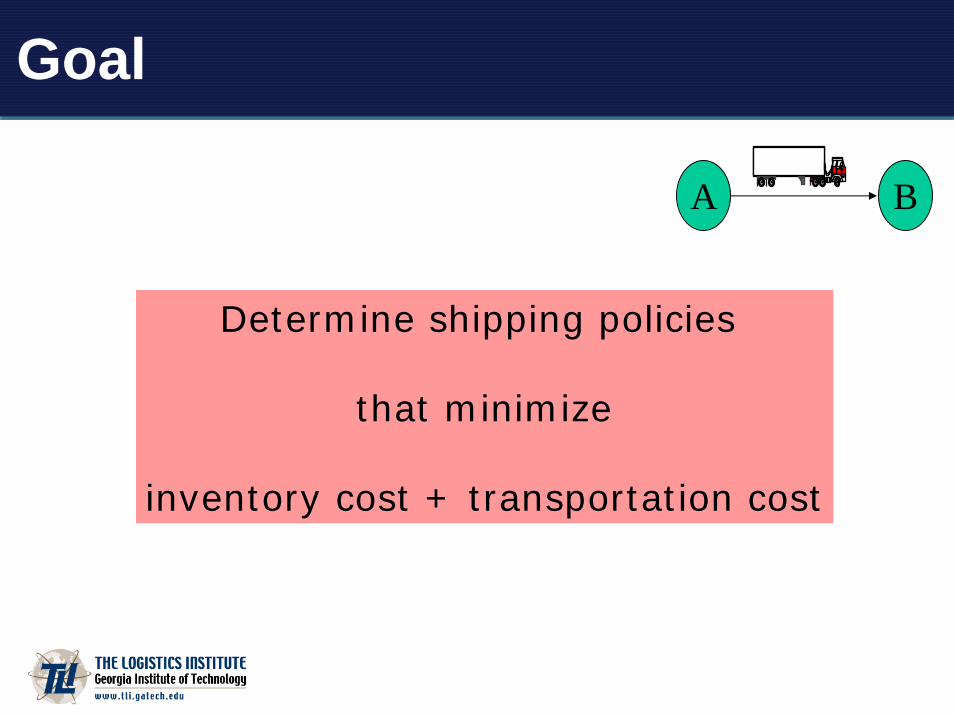
Deterministic order-up-to level policy

• Each customer defines a minimum and a maximum level of the inventory

• The plant determines the set of delivery time instants

• Every time a customer is visited, the shipping quantity is such that the maximum level of the inventory is reached at the customer

Order-Up-ToInventory at retailer s Maximum

level

Time

Us

Minimumlevel

Ls

Startinglevel

Problem FormulationDecisions:

• For each customer s:the set of delivery time instants

For each delivery time instant t:the route followed by the vehicle

Objective function:

Min Inv. Plant + Inv. Customer + Routing

Key Assumption: Deliveries are instantaneous

Transportation Costs

Inventory Routing Problem

• Single Plant

– single facility

– single product

– set of n customers

– set of m homogenous vehicles of capacity Q

Inventory Routing Problem

• Each customer:

– storage capacity

– initial inventory

– product usage rate OR– probability distribution of product

usage

Inventory Routing Problem

• Objective – Minimize distribution costs without

causing any stock-outs over a finite horizon OR

– Maximize the expected total discounted value (rewards minus costs) over an infinite horizon

Inventory Routing Problem

• Extensions– Operating modes– Delivery time windows– Delivery times (fixed plus variable part)

Inventory RoutingEven simple situations are non-trivial

There are 14 possible customer combinations

A-B-C-D A-BA-B-C A-CA-B-D A-DA-C-D B-CA B-DB C-DC D

There are an infinite number of possible delivery volumes

10

100

10

140

C

D

100

100

100

A B

A B C D

Daily Use 1000 3000 2000 1500

Max. Delv. 5000 3000 2000 4000

Truck capacity is 5000

Inventory Routing

10

100

10

140

C

D

100

100

100

A B

A B C D

Daily Use 1000 3000 2000 1500

Max. Delv. 5000 3000 2000 4000

Truck capacity is 5000

The “natural” solution

Daily scheduletrip 1: deliver 1000 to A & 3000 to Btrip 2: deliver 2000 to C & 1500 to D

420 miles per day

A better solution

Day 1 scheduletrip 1: deliver 3000 to B & 2000 to C

Day 2 scheduletrip 1: deliver 2000 to A & 3000 to Btrip 2: deliver 2000 to C & 3000 to D

380 miles per day

Complexity

• Single customer problem?• Two customer problem?

Single Customer Problem

Planning horizon

Usage rate

Initial inventory

Deterministic d-day policy

vT (d) = max(0, d Tu−Imin(C,Q)e)c

Storage capacity

Vehicle capacity

Single Customer Problem

Stochastic d-day policy

Cost of filling up every d days over T day period:

d ≤ T : vT (d) =Pd−1

j=1 pj(vT−j(d) + S) + (1− p)(vT−d(d) + c)

d > T : vT (d) =PTj=1 pj(vT−j(d) + S)

Probability that stockout occurs on day jStockout cost

Probability that no stockout occurs

Delivery cost

vT (d) = α(d) + β(d)T + f(T, d)

α(d) constant, f(T,d) goes to zero exponentially fast as T → ∞

β(d) = pS+(1−p)cPdj=1 jpj

Single Customer Problem

An optimal constant replenishment period strategy over a large T-day planning period will correspond to choosing d* to minimize β(d)

β(d) = pS+(1−p)cPdj=1 jpj

Expected number of days between deliveries

Expected cost of a delivery

Best d-day policy

Demand: uniformly in [1,20]Deliver cost: 40Stockout cost: 50

Optimal policy

Two customer problem

Deterministic d day policy:

Always individually:

Always together:

Sometimes individually, sometimes together?What if one cannot take a full truckload?What if the customers are close together?How much to deliver to each of them on a combined route?

Two Customer Problem

• Stochastic policy:– Storage capacity: 20– P[demand = 0] = 0.4, P[demand = 10] = 0.6– Shortage penalty: 1000 customer 1; 1005 customer 2– Vehicle capacity: 10– Individual routes: 120; Combined route: 180

• Infinite horizon Markov Decision Process– Minimize expected total discounted cost

Two Customer Problem

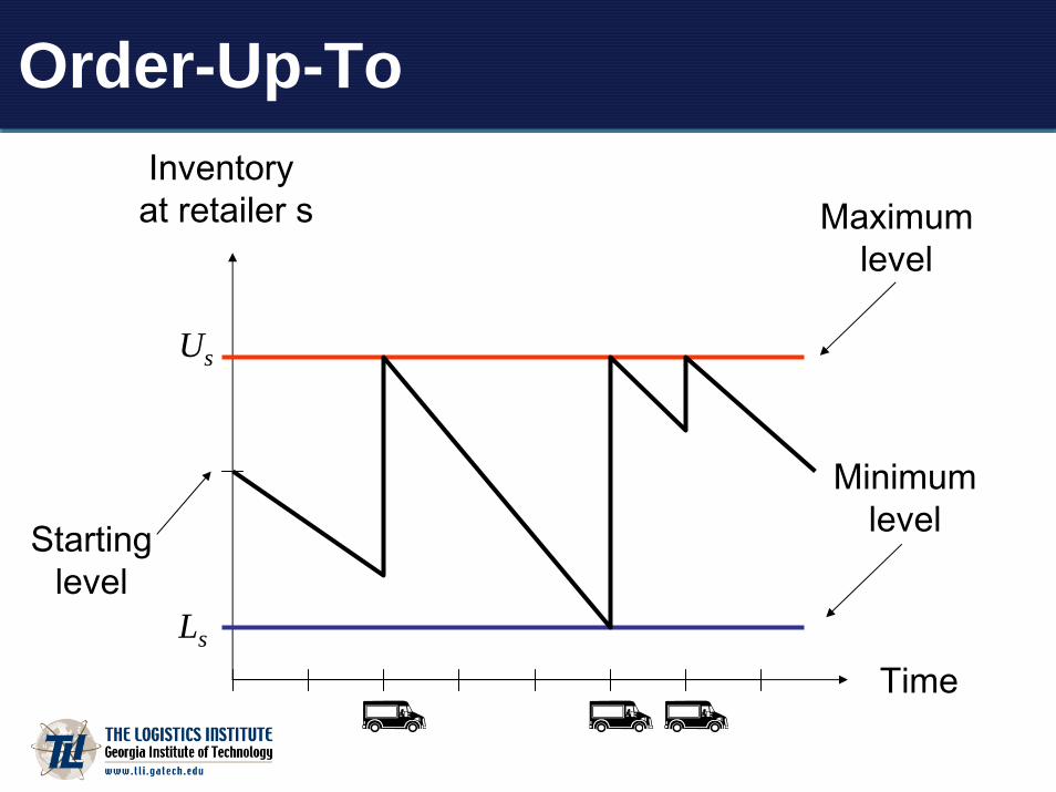
Bounds

Customer usage during period: ui

Customer storage capacity: Ci

Vehicle capacity: Q

Minimize total mileage D*

subject to

Total volume delivered to customer i ui

Maximum volume delivered per trip Q

Maximum quantity delivered to customer i min(Ci, Q)

Bounds

Simple bounds on total mileage

Assume Ci ≥ Q

ui

I

Q

tij

Set of customers

Usage of customer i (period)

Vehicle tank capacity

Travel distance from i to jAssume direct delivery

Two Customer Analysis

1 201t 12t

120102 ttt +=

QC >1

QC <2

0

Plant

Customer

Patterns:

(Q,0)

(0,C2)

(Q-C2,C2)

Two Customer Analysis

Plant

Customer01t12t

02t

QC <1

QC >20

1

2

Assume :Patterns:

(C1,0)

(0,Q)

(C1,Q-C1)

Extra mileage

Improved BoundsDelivery Patterns

Pj = (dj1,dj2, ..., djn) is feasible if

≤∑i ∈ I dji Q ≤ ≤0 dji Ci ∀ i ∈ I .andδ(Pj) = {i∈ I : dji > 0} : Customers visited in Pj

c(Pj) : The cost of delivery pattern Pj - optimal TSP value P : Set of all feasible delivery patterns

Pattern Selection LP

D* = min ∑Pj ∈ P c(Pj) xj

s.t. ∑Pj ∈ P dji xj ≥ ui, ∀ i ∈ I

xj ≥ 0

xj : How many times should pattern Pj be used

Obstacles

Obstacle I : Infinite number of feasible delivery patterns

Obstacle II : The calculation of the cost of each delivery pattern involves the solution of a traveling salesman problem

Obstacle I

Base Pattern A feasible delivery pattern P is a base pattern if at most one customer, say k, in δ(P) receives a delivery quantity less than min(Ck, Q), and, in that case, the delivery quantity is Q – ∑i ∈ δ(P)\k Ci

Theorem

The base patterns are sufficient to find an optimal solution to the Pattern Selection LP

Number of columns of Pattern Selection LP is finite

Obstacle IIFocus on upper and lower bounds on D* instead of D* itself.Lower bound (LBk) : If Ci < Q/k, then assume Ci = Q/k

LB1 ≤ LB2 ≤ … ≤ D*

If mini∈ I(Ci) ≥ Q/k, then LBk = D*

|δ(P)| ≤ k for any base pattern P

Upper bound (UBk) : At most k stops in a tour

For values k=3 and k=4, the TSPs that have to be solved involve at most 4 and 5 stops, respectively, and thus can be solved relatively easily by enumeration

UB1 ≥ UB2 ≥ … ≥ D*

If ⎡ Q/mini∈ I(Ci) ⎤ ≤ k, then UBk = D*

|δ(P)| ≤ k for any base pattern P

DominanceDo we need base pattern P ?

If z ≤ c(P),

then the base patterns with λj > 0 collectively dominate P

Base pattern P can be eliminated from the Pattern Selection LP

Simple DominanceConsider base pattern P with d4<C4

P

C1C2C3d4

d44 = min(Q,C4 )

C1C2C3

0

000

d44

Condition I

C1C2C3

0

C100

d14

0C20

d24

0

C3

0

d34

di4 = min(Q-Ci,C4 )

Condition II

C1C2C3

0

C1

0d124

C2

0

C3d234

C20

d134

C1

C3

dij4= min(Q-Ci -Cj,C4 )

Condition III

Instances n before after1 136 5,015,046 3,029,9802 157 7,665,722 4,336,4663 169 9,086,385 5,420,9074 147 15,180,701 8,838,1375 157 14,471,228 8,975,6156 194 22,575,528 16,640,122

Implementation: Sifting Approach

Specialized solver for LPs with a large ratio of number of columns to number of rows

A Partial LP

Subset of full set of columns

Check reduced costs for the remaining columns

Optimal solution

Instance n # of patterns # of iterations default(sec) sifting(sec)1 136 3,029,980 5 85.66 77.092 157 4,336,466 6 118.37 121.343 169 5,420,907 6 155.29 152.564 147 8,838,137 5 360.20 240.835 157 8,975,615 6 397.33 254.816 194 16,640,122 6 675.98 533.56

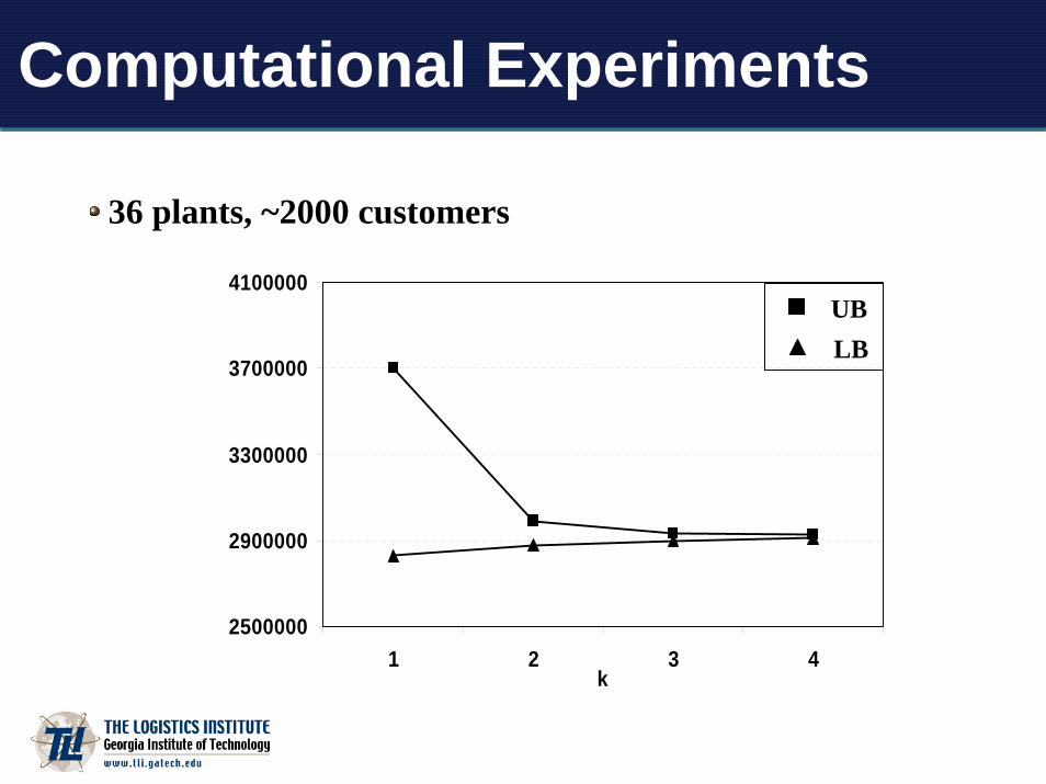
Computational Experiments

36 plants, ~2000 customers

2500000

2900000

3300000

3700000

4100000

1 2 3 4k

UBLB

Inventory RoutingSchedule 1: 420 miles per day

10

100

10

140

3

4

100

100

100

1 2

(1000,3000,0,0),(0,0,2000,1500)

Schedule 2: 380 miles per day(0,3000,2000,0)(2000,3000,0,0), (0,0,2000,3000)

Pattern Selection LP with T=1dayOptimal Objective Value : 380

0.5 : (0,3000,2000,0)0.5 : (2000,3000,0,0)0.5 : (0,0,2000,3000)

Pattern Selection LP found schedule 2 and it shows no better schedule exists!Q = 5000

Solution Approaches

• Deterministic– Based on average product usage

• Stochastic– Based on probability distribution of product

usage

Deterministic Solution Approach

Two Phase Approach– Phase I: Determine which customers should

receive a delivery on each day of the planning period and how much

– Phase II: Create the precise delivery routes for each day

Rolling horizon approach

Deterministic Solution Approach

Two Phase Approach–Phase I: Integer program–Phase II: Insertion heuristic

Integer ProgramLower bound on the total volume that has to be deliveredto customer i by the end of day t:

Upper bound on the total volume that can be deliveredto customer i by the end of day t:

Delivery constraint:

Integer Program

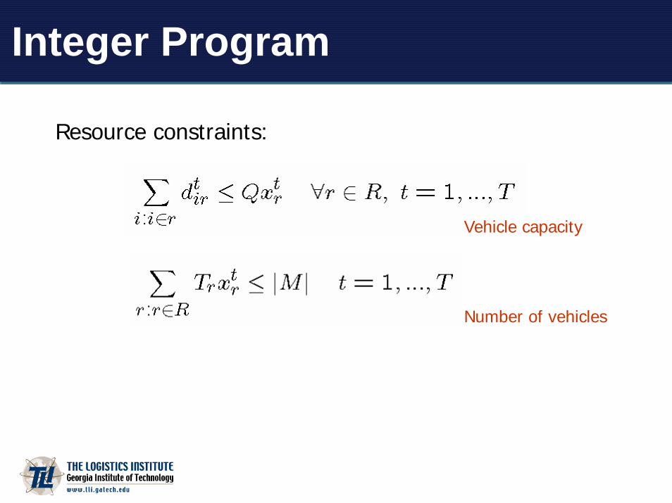
Resource constraints:

Vehicle capacity

Number of vehicles

Integer Program

Vehicle capacity

Number of vehicles

Storage capacity

Integer Program

Improve the efficiency by

– Route elimination– Aggregation

Insertion Heuristic

• Input for next k days:– List of customers– List of recommended delivery amounts

• Output for next k days for each vehicle:– Start time– Sequence of deliveries– Arrival time at each customer– Actual delivery amount at each customer

Key Issue

• How to handle variable delivery quantities?– We may be able to increase delivery amounts – We may be able to decrease delivery

amounts– We may be able to postpone deliveries to

another day

Insertion Heuristic

Minimum delivery volume:Amount suggested by the integer program

Earliest time a delivery can be made:

Insertion HeuristicLatest time a delivery can be made:

Maximum delivery volume:

Insertion Heuristic

For each route:– Earliest time a route can start– Latest time a route can start– Earliest time a route can end– Latest time a route can end– Sum of minimum deliveries– Sum of maximum deliveries

Insertion Heuristic

Feasibility check:– Compute minimum delivery volume. Will the

minimum delivery volume fit given the other deliveries?

– Compute earliest and latest delivery can take place. Is late greater than early?

– Compute maximum delivery volume. Is minimum less than maximum?

Delivery Volume Optimization

• Observe:– The amount that can be delivered at a customer

depends on the time at which the delivery starts– The time it takes to make the delivery depends on the

size of the delivery– There is a limit on the elapsed time of a route

• Result:– It is nontrivial to determine, given a route, i.e., a

sequence of customer visits, what the maximum amount of product is that can be delivered on this route !!

Delivery Volume Optimization

Tank capacity or Truck capacity

Earliest delivery time Latest delivery time

Usage rate Pump rate

Delivery Volume Optimization

• There is a polynomial time algorithm that solves this problem. The algorithm constructs a series of piecewise linear graphs (one for each customer on the route) representing the maximum amount of product that can be delivered on the remainder of the route as a function of the start time of the delivery at the customer.

Delivery Volume Optimization

Customer 1

Customer 2

Delivering a little less at Customer 1 allows a much larger delivery at Customer 2

Pump time +Travel time

GRASP

• The insertion heuristic is embedded in a Greedy Randomized Adaptive Search Heuristic (GRASP)

Stochastic IRP

Determine inventory

levels

Assign customers to vehicles

Deliver at customer & drive back

Load to capacity & drive

to customer

Markov Decision Process Model

• State, x

– inventory levels at different customers

• Action, a– Which customers to replenish

– How much to deliver at each customer

– How to combine customers into vehicle routes

• Objective

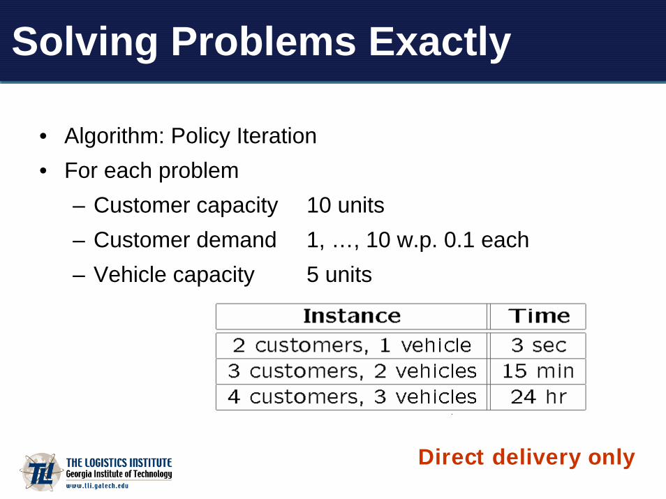
Solving Problems Exactly

• Algorithm: Policy Iteration• For each problem

– Customer capacity 10 units– Customer demand 1, …, 10 w.p. 0.1 each– Vehicle capacity 5 units

Direct delivery only

MDP Model: Issues

• Optimality Equation

• Computing optimal value function• Computing expected value• Computing optimal action

V ∗(x) = maxa∈A(x)E[g(x, a) + αV ∗(Xt+1)|Xt = x,At = a]

Approximation Methods• Idea

Approximate V ∗ with V̂

• Motivation

• Parameterized approximation function

Examples for Basis Functions• Polynomial function

– inventory level at customers– second order effects

4450

4650

4850

5050

5250

0 1 2 3 4 5 6 7 8 9 10

Inventory at customer 3 (X3)

Val

ue

opt, X2 = 0

opt, X2 = 5

opt, X2 = 10

app, X2 = 0

app, X2 = 5

app, X2 = 10

Approximating the Value Function

• Although IRP is not separable, the major costs (including transportation) are associated with small groups of customers (vehicle routes)

• We do not know in advance which groups will be in each vehicle route

• We can identify subsets of customers that can possibly be in the same vehicle route

MDP for subset of customers

• State, (xi, ki)– inventory at customers × vehicles

which could be allocated• Action, ai

– deliveries to customers in the subset• Transition probability

MDPs for small subsets of customers can be solved optimally in advance

Approximating the Value Function

• In advance, optimally solve problems for subsets of customers

• On each day, partition the customers and vehicles into subsets by solving a cardinality constrained partitioning problem

• 1-customer subsets: nonlinear knapsack problem

• 2-customer subsets: maximum weight perfect matching problem

Non-linear Knapsack Problem

Vehi

cles

Customers

0,0

2,0

1,1

2,1

1,0

0,1 0,3

2,3

1,3

0,2

1,2

2,2

0

V1(x1,0)

V1(x1,0)

V1(x1,0)

V1 (x

1 ,2)

V2 (x

2 ,1)

V2(x2,0)

V2(x2,0)

V3(x3,0)

V3 (x

3 ,2)

0

0

V3 (x

3 ,1)

V3(x3,0)0 0

0

0

0

0

0

0

0

Computing ParametersMethod I

• Objective Function

• Looks like weighted least squares regression problem

Cannot be computed for

large problems

Computing ParametersStochastic Approximation Algorithm

π• Simulate system under policy

• Sample path x0, x1, …, xt, ...

• Update coefficients

• Step size

• Temporal difference

• Eligibility vectorδt = g(xt,π(xt)) + αV̂ (xt+1, rt)− V̂ (xt, rt)

P∞t=0 γ

t =∞, P∞t=0(γt)2 <∞zt+1 = αλzt + OrV̂ (xt, rt)

Convergence typically very slow

Computing ParametersMethod II

• Value function for policy

• Looks like weighted least squares regression problem

Cannot be computed for

large problems

π

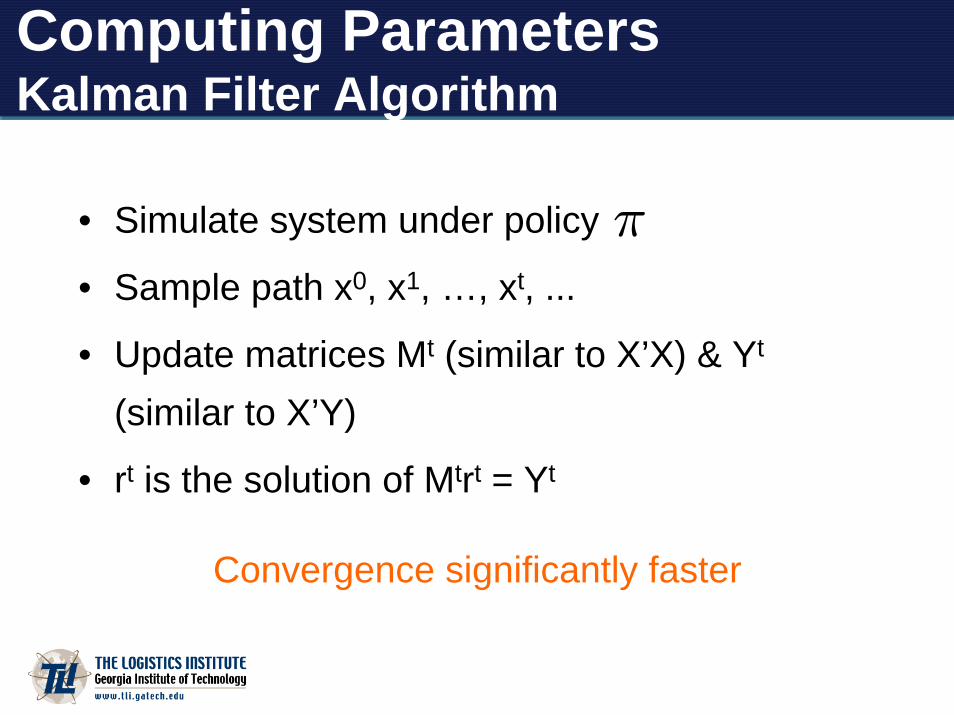
Computing ParametersKalman Filter Algorithm

• Simulate system under policy

• Sample path x0, x1, …, xt, ...

• Update matrices Mt (similar to X’X) & Yt

(similar to X’Y)

• rt is the solution of Mtrt = Yt

π

Convergence significantly faster

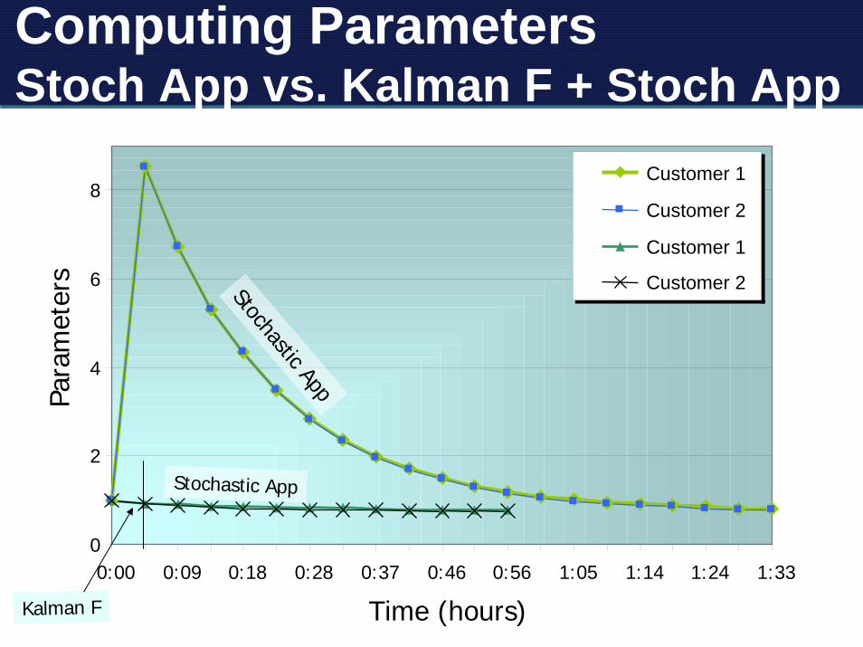
Computing ParametersStoch App vs. Kalman F + Stoch App

0

2

4

6

8

0:00 0:09 0:18 0:28 0:37 0:46 0:56 1:05 1:14 1:24 1:33

Time (hours)

Para

met

ers

Customer 1

Customer 2

Customer 1

Customer 2Stochastic App

Stochastic App

Kalman F

Estimating Expected Value

• Multi-dimensional Integral– d = #dimensions = #customers– very hard to compute

• Deterministic Methods– MSE = O(n2 - 2c/d)

• Randomized Methods– MSE = O(1/n)

• Deterministic methods are better when 2 - 2c/d < -1

Randomized methods are better for large d

Choosing the Best Action

• Based on sample averages of actions• Question

– How large should the sample be so that we are reasonably sure of choosing the best action?

• Nelson and Matejcik (1995)– Sample size to ensure chosen alternative has value within

tolerance of best value with specified probability• Variance reduction methods

– Common random numbers– Orthogonal arrays

Variance Reduction MethodsNumber of Observations for Choosing Best Action

0

400

800

1200

1600

2000

1 101 201 301 401 501 601 701 801 901

Simulation Steps

Num

ber

of O

bser

vatio

ns

OARandom

Approximate Policy Iteration

1. Initialization. Simulate initial policy π0 and obtain parameters rπ0

2. Use parameters rπt−1 for policy πt and obtain actions using

3. Simulate policy πt and obtain parameters rπt

4. t← t+ 1; go to Step 2

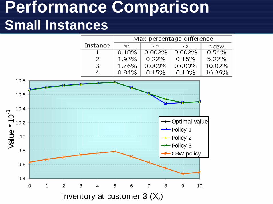
Performance ComparisonSmall Instances

9.4

9.6

9.8

10

10.2

10.4

10.6

10.8

0 1 2 3 4 5 6 7 8 9 10

Inventory at customer 3 (X3)

Valu

e *1

0-3

Optimal valuePolicy 1Policy 2Policy 3CBW policy

Performance ComparisonLarge Instances

Price-Direct Replenishment

• A control policy based on a simple economic mechanism for dispatching

• The dispatcher receives a transfer price diVi from management for replenishing diunits of product at customer i.

• The dispatcher is responsible for paying the distribution costs cI, when replenishing a set of customers I.

Price-Direct Replenishment

• Net value for dispatcher

• Incremental value for dispatcher

Pi∈I Vidi − cI

diVi − (cI∪{i}cI)

Price-Directed Replenishment

• Management’s problem: Set Vi so that the dispatcher is motivated to minimize the long-run time average replenishment costs

Price-Direct Replenishment

• Management problem (single customer):

Primal Dual

min cZ

dZ = u

0 ≤ d ≤ min{C,Q}0 ≤ Z

maxuV

dV ≤ c ∀0 ≤ d ≤ min{C,Q}

replenishmentfrequency

usage

Price-Direct Replenishment

• Management problem (single customer):

Dual

maxuV

dV ≤ c ∀0 ≤ d ≤ min{C,Q}

If V is interpreted as the transfer price received by the dispatcher for replenishing one unit, then this dual program maximizes the rate at which transfer revenue accumulates, subject to the constraint that the total transfer payment cannot exceed the cost on any replenishment

Direct Replenishment

• Price directed operating policy maximizing the net value of a replenishment

max0≤d≤min{C,Q}{V ∗d− c}

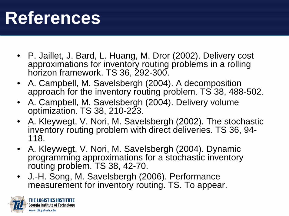
References

• P. Jaillet, J. Bard, L. Huang, M. Dror (2002). Delivery cost approximations for inventory routing problems in a rolling horizon framework. TS 36, 292-300.

• A. Campbell, M. Savelsbergh (2004). A decomposition approach for the inventory routing problem. TS 38, 488-502.

• A. Campbell, M. Savelsbergh (2004). Delivery volume optimization. TS 38, 210-223.

• A. Kleywegt, V. Nori, M. Savelsbergh (2002). The stochastic inventory routing problem with direct deliveries. TS 36, 94-118.

• A. Kleywegt, V. Nori, M. Savelsbergh (2004). Dynamic programming approximations for a stochastic inventory routing problem. TS 38, 42-70.

• J.-H. Song, M. Savelsbergh (2006). Performance measurement for inventory routing. TS. To appear.

References

• L. Bertazzi, M.G. Speranza (2002). Continuous and discrete shipping strategies for the single link problem. TS 36, 314-325.

• L. Bertazzi, G. Palletta, M.G. Speranza (2002). Deterministic order-up-to level policies in an inventory routing problem. TS 36, 119-132.

• L. Bertazzi, G. Palletta, M.G. Speranza (2005). Minimizing the total cost in an integrated vendor-managed inventory system. JH 11, 393-419.

References

• D. Adelman (2003). Price-directed replenishment of subsets: methodology and its application to inventory routing. MSOM 5, 348-371.

• V. Gaur, M. Fisher (2004). A periodic inventory routing problem at a supermarket chain. OR 52, 813-822.

• A. Campbell, J. Hardin (2005). Vehicle minimization for periodic deliveries. EJOR 165, 668-684.

• W. Bell, L. Dalberto, M. Fisher, A. Greenfield, R, Jaikumar, P. Kedia, R. Mack, P. Prutzman (1983). Improving the distribution of industrial gases with an online computerized routing and scheduling optimizer. Interfaces 13, 4-23.

Inventory Routing Game

• http://kronos.isye.gatech.edu:8081/IRGame• Login: player1, …, player20• Password: player1, …, player20• Play Instance 3

• Winner gets prize on Friday…

Questions?