Invasive forest pest surveillance: surveydevelopment and reliability

John W. Coulston, Frank H. Koch, William D. Smith, and Frank J. Sapio

Abstract: Worldwide, a large number of potential pest species are introduced to locations outside their native ranges;under the best possible prevention scheme, some are likely to establish one or more localized populations. A comprehen-sive early detection and rapid-response protocol calls for surveillance to determine if a pest has invaded additional loca-tions outside its original area of introduction. In this manuscript, we adapt and spatially extend a two-stage samplingtechnique to determine the required sample size to substantiate freedom from an invasive pest with a known level of cer-tainty. The technique, derived from methods for sampling livestock herds for disease presence, accounts for the fact thatpest activity may be low at a coarse spatial scale (i.e., among forested landscapes) but high at a fine scale (i.e., within agiven forested landscape). We illustrate the utility of the approach by generating a national-scale survey based on a riskmap for a hypothetical forest pest species threatening the United States. These techniques provide a repeatable, cost-effective, practical framework for developing broad-scale surveys to substantiate freedom from non-native invasive forestpests with known statistical power.

Resume : A travers le monde, un grand nombre d’especes de ravageurs potentiels sont introduites dans des endroits situesen dehors de leur aire de repartition naturelle. Malgre la meilleure strategie possible de prevention, certains de ces rava-geurs ont des chances d’etablir une ou plusieurs populations localisees. Un protocole complet de detection precoce et dereaction rapide demande une surveillance pour determiner si un ravageur a envahi d’autres endroits a l’exterieur de sazone d’introduction originelle. Dans cet article, nous adaptons une methode d’echantillonnage en deux temps et lui ajou-tons une dimension spatiale afin de determiner la taille de l’echantillon necessaire pour confirmer l’absence d’un ravageurinvasif avec un degre de certitude connu. La methode est derivee des methodes d’echantillonnage des troupeaux de betailpour detecter la presence de maladies et tient compte du fait que l’activite des ravageurs peut etre faible a une echelle spa-tiale grossiere (c.-a-d. parmi des paysages forestiers) mais elevee a une echelle plus fine (c.-a-d. a l’interieur d’un paysageforestier). Nous illustrons l’utilite de l’approche en generant un inventaire a l’echelle nationale base sur une carte de ris-ques pour une espece de ravageur forestier hypothetique qui menacerait les Etats-Unis. Ces techniques offrent un cadrepratique, reproductible et peu couteux pour elaborer des inventaires a grande echelle afin de confirmer l’absence de rava-geurs forestiers exotiques et invasifs avec une puissance statistique connue.

[Traduit par la Redaction]

Introduction

Non-native invasive species pose a significant threat tonatural resources worldwide. Resource losses, environmentaldamages, and control costs in the United States due to inva-sive species have been recently estimated to exceed US$120

billion/year (Pimentel et al. 2005). In particular, non-nativeinsects and diseases affecting US forests have an estimatedimpact of greater than US$4.3 billion annually in damagesand control expenditures (Pimentel et al. 2005). Annual con-trol costs for individual invasive species can exceed severalmillion US dollars, although forgoing control efforts may ul-timately cost much more; without active management, inva-sives that are currently limited in geographic distribution canrapidly become established over large areas and, sub-sequently, cause extensive environmental degradation(Chornesky et al. 2005; Lodge et al. 2006). Historically, in-vasives have been responsible for severe impacts to forestfoundation species such as jarrah (Eucalyptus marginataDonn ex Sm.) in Western Australia or the American chest-nut (Castanea dentata (Marsh.) Borkh.), which has beennearly eliminated from US forests (Ellison et al. 2005;McDougall et al. 2002). These impacts result in major com-positional changes that affect wildlife and overall ecosystemprocesses (Chornesky et al. 2005; Ellison et al. 2005). Fur-thermore, invasives place added pressure on many criticallyimperiled animal and plant species through competition orpredation (Wilcove et al. 1998).

In the United States, Executive Order 13112 established aNational Invasive Species Council and mandated that federal

Received 22 October 2007. Accepted 2 June 2008. Published onthe NRC Research Press Web site at cjfr.nrc.ca on 19 August2008.

J.W. Coulston.1 US Forest Service, Southern Research Station,4700 Old Kingston Pike, Knoxville, TN 37919, USA;Department of Forestry and Environmental Resources, Box8008, North Carolina State University, Raleigh, NC 27695,USA.F.H. Koch. Department of Forestry and EnvironmentalResources, Box 8008, North Carolina State University, Raleigh,NC 27695, USA.W.D. Smith. US Forest Service, Southern Research Station,3041 Cornwallis Road Research Triangle Park, NC 27709, USA.F.J. Sapio. US Forest Service, Forest Health TechnologyEnterprise Team, 2150 Centre Ave, Building A, Suite 331, FortCollins, CO 80526, USA.

1Corresponding author (e-mail: jcoulston@fs.fed.us).

2422

Can. J. For. Res. 38: 2422–2433 (2008) doi:10.1139/X08-076 # 2008 NRC Canada

agencies whose activities influence the status of invasivespecies will ‘‘detect and respond rapidly to and control pop-ulations of such species in a cost-effective and environ-mentally sound manner’’ and ‘‘monitor invasive speciespopulations accurately and reliably’’ (Clinton 1999,p. 6184). Similarly, a 2006 report from the Ecological Soci-ety of America (ESA) highlighted potential impacts ofinvasive species and provided several key policy recommen-dations, including coordinated efforts to detect invasionswhile they are still localized, better enabling eradication ofspecies before they become established (Lodge et al. 2006).The report acknowledged the high costs of surveying forrare individuals and, therefore, emphasized the cost-effectiveness of surveillance techniques that focus on loca-tions with high invasion risks. Demonstrating the trulyglobal scope of the invasive pest problem, both ExecutiveOrder 13112 and the ESA report echo procedures and poli-cies outlined in the International Standards for PhytosanitaryMeasures (ISPM) produced under the International PlantProtection Convention. In addition to general surveillanceguidelines, ISPM publications address requirements for thedetermination of an area’s pest status as well as conditionsfor establishing pest-free or low-pest-prevalence areas (FAO1995, 1997, 1998, 2005).

Pest surveillance is a complex task, particularly at a na-tional or similarly broad spatial scale. This is especially truefor forest pests, which can travel, often cryptically, along awide variety of pathways. Every year, a large number ofnon-native insects and diseases affecting forest tree speciesare intercepted at international ports of entry from commer-cial shipments of live plants, logs and raw wood products,and other commodities, as well as in packing materials andeven in airline passenger baggage (see Brockerhoff et al.2006; Haack 2003; Liebhold et al. 2006; McCullough et al.2006; Tkacz 2002; Work et al. 2005). Pests that evade theinspection process may be accidentally introduced into for-ested areas. Potentially serious non-native pests that have re-cently made inroads into US forests include sudden oakdeath (caused by Phytophthora ramorum Werres et al.), firstdetected in 1995; the emerald ash borer (Agrilus planipennisFairmaire), first detected in 2002; and the sirex woodwasp(Sirex noctilio F.), which was first detected in the UnitedStates in 2005 (Hoebeke et al. 2005; Ivors et al. 2006;McCullough and Katovich 2004). Internationally, note-worthy examples include the pine wood nematode (Bursa-phelenchus xylophilus (Steiner & Buhrer) Nickle), native toNorth America but now established in eastern Asia and alsoreported in Portugal in 1999, as well as the red turpentinebeetle (Dendroctonus valens LeConte), a secondary pest ofpines in its native North American range that has causedwidespread tree mortality in China since it was first detectedin 1998 (Brockerhoff et al. 2006; Mota et al. 1999; Schraderand Unger 2003; Yan et al. 2005).

Typically, invasive pests like those just mentioned are in-troduced to a new country or region at one or no more thana few specific points. However, through both natural andhuman-mediated pathways (e.g., interstate transportationcorridors), they may be subsequently dispersed at multiplespatial scales. In particular, human-mediated pathways mayfacilitate the rapid spread of a pest species to previously re-mote locations (NRC 2002; Chornesky et al. 2005). This

multiple-scale dispersal pattern results in a clustered geo-graphic distribution of the pest among landscapes (where alandscape is simply an area of some specified size that canserve as a sampling unit for a broad-scale spatial survey).Generally, the proportion of all landscapes that are invadedis low with a newly introduced pest, yet within an invadedlandscape, the density within the area actually occupied oraffected by the pest can be high. Given that conducting acomplete census is cost-prohibitive, a probabilistic approachmay instead be used to substantiate freedom from a pestspecies at an acceptable level of certainty. Such a probabil-istic approach is consistent with ISPM guidelines for tar-geted surveys of recently introduced pests (FAO 1997).

Scientifically sound surveillance techniques are prerequi-site to any broad-scale efforts to combat invasive species(Lodge et al. 2006; Rajan 2006). A well-developed surveil-lance system facilitates early detection, increasing the win-dow of opportunity to initiate management measures (Rajan2006; Venette et al. 2002). A primary objective of this paperis to document techniques that can be used to estimate therequired sample size of surveys to substantiate freedomfrom non-native forest pests with known reliability. To ac-complish this, we extend the one-dimensional methods ofCameron and Baldock (1998) to the spatial domain withvector data; chiefly, we develop a model to calculate theparameters necessary to estimate sample size. We providean example to illustrate surveillance methodology by (i) de-fining the population of interest and sample frame, (ii) set-ting standards of statistical confidence and certainty, (iii)determining the optimal sample size, and (iv) using the sam-ple size to create the detection survey scheme.

Methods

Our methodology is intended for cases where a recentlyintroduced forest pest has been found in only a small portionof its estimated potential range. In general, invasions are un-predictable, making it difficult to accurately model theirprogress or ultimate extents (Kareiva et al. 1996). Nonethe-less, analyses that focus on the simpler task of identifyingareas with heightened invasion risk may inform the designof cost-effective survey programs for early detection(Andersen et al. 2004, FAO 1997; Kareiva et al. 1996). For-est pest risk maps (e.g., Downing et al. 2005; Kelly et al.2007; Koch et al. 2006; Poland and McCullough 2006) areanalytical combinations of spatial data from three categoriesthat represent where a pest is most likely to be introducedand (or) established: host species distribution, climatic orother environmental constraints, and pathways of pest move-ment (Bartell and Nair 2004). Because of a lack of qualitydata, some risk maps omit one or more of these categories,but all serve the same basic purpose: to provide a relativerisk rating for all locations within the geographic area of in-terest, thus indicating where resources for monitoring orother measures should be prioritized.

Risk maps have several applications, but here we use arisk map to define the population of interest (i.e., the at-riskforest area) and to construct the sampling frame based on aglobal sampling grid (White et al. 1992). However, we mustalso decide upon the appropriate sampling technique and re-quired level of certainty before determining the required

Coulston et al. 2423

# 2008 NRC Canada

sample size (Cochran 1977). When considering the surveil-lance of invasive forest pests, two-stage samples are attrac-tive because we expect the species of interest to clusterwithin the primary sampling units. That is, we expect thelikelihood of species occurrence within primary samplingunits to be more similar than the likelihood among primarysampling units. Therefore, to take advantage of this cluster-ing, it makes sense economically to use a two-stage sample(Reilly 1996). Our aim is to use the global sampling ap-proach developed by White et al. (1992) to construct ourprimary sampling units and develop appropriate techniquesto determine the stage-two (within primary sampling unit)sample when the stage-two sample unit is a pheromone trapor similar device.

Two-stage sample size formulaCameron and Baldock (1998) developed a probability for-

mula to estimate the necessary sample size for two-stagesampling where the purpose of the survey is to substantiatefreedom from disease at given levels of sensitivity and con-fidence. They developed their formula under the scenario ofsampling animal herds over large areas where diseased ani-mals are considered to cluster within a herd. Such clusteringwithin a herd often occurs because the distribution of dis-ease agents is unbalanced across the population. This is es-pecially true with rare diseases, where the among-herdinfection rate may be low, but within a diseased herd, theinfection rate can be quite high. Their equation for the prob-ability of observing at least one event (e.g., diseased animal)is

½1� P ¼ 1� �1 PðS�2 jSþ1 Þ� �n2 þ ð1� �1Þ

� �n1where P is the probability of observing at least one event, orthe level of certainty; �1 is the stage-one prevalence, or pro-portion of stage-one sampling units in which the event oc-curs, which is also the probability of selecting a stage-onesampling unit with the event; PðS�2 jSþ1 Þ is the conditionalprobability of failing to observe the event based on the sec-ond stage sample (S�2 ) given that the event does occur in theselected stage-one sampling unit (Sþ1 ); n2 is the number ofsamples within each primary sampling unit; (1 – �1) is theprobability of selecting a stage-one sampling unit where theevent does not occur; and n1 is the number of stage-onesampling units. Equation 1 can be rearranged to solve forthe sample size required to stipulate freedom from an event

½2� n1 ¼ln ð1� PÞ

ln �1 PðS�2 jSþ1 Þn2� �

þ ð1� �1Þ� �

where P is the level of certainty specified a priori and �1 isspecified a priori.

Cameron and Baldock (1998) developed eq. 2 to calculatethe required sample size to substantiate freedom from dis-ease in large animal herds. The approximation of PðS�2 jSþ1 Þfor large herd sizes was provided by Cannon and Roe(1982):

½3� PðS�2 jSþ1 Þ ¼ 1� �2

Na � n2�12

!

where �2 is the stage-two prevalence or, in this case, the

number of diseased animals in a herd (set a priori); Na isthe mean number of animals in a herd; and n2 is the numberof samples within each primary sampling unit; in this case,the number of animals sampled within the herd.

There are many combinations of n1 and n2 that will pro-duce the required level of certainty, and there are often dif-ferent costs associated with the stage-one sample and thestage-two sample (Clark and Steel 2000; Waters and Chester1987). Cameron and Baldock (1998) suggested usingCochran’s (1977) cost function to select the values of n1and n2 that minimize the overall cost of the survey. Thecost function takes the following form:

½4� Ctotal ¼ C1 � n1 þ C2 � n2 � n1

where Ctotal is the total cost of the survey; C1 the cost of ob-taining each stage-one sample; and C2 is the cost of obtain-ing each stage-two sample. The combination of n1 and n2that minimizes Ctotal is the optimal solution.

The formulations provided by Cameron and Baldock(1998) and Cannon and Roe (1982) are based on discretecounts and assume samples are drawn from an infinite pop-ulation. In the case of invasive pest surveillance, changesmust be made to adequately estimate the conditional proba-bility PðS�2 jSþ1 Þoutlined in eqs. 1, 2, and 3; this is due to thespatial nature of the sampling problem. Also, depending onhow the stage-one sample is defined, the sampling fractionmay be so large that assuming an infinite population is inad-equate.

Adjustment to the stage-two probabilityRather than sampling individuals, a detection mechanism

(e.g., a pheromone trap or similar device; hereafter, we usethe term ‘‘trap’’) is typically used for pest surveillance, withthe purpose of determining whether a pest is present in anarea of interest. When traps are employed, the samplingproblem becomes spatial in character, and subsequently, we

Fig. 1. The additional area (z) that should be accounted for whenestimating PðS�2 jSþ1 Þ given the infected area (�2) and the trap area(A2).

2424 Can. J. For. Res. Vol. 38, 2008

# 2008 NRC Canada

must develop a new approach to estimate PðS�2 jSþ1 Þ). In thetwo-dimensional case, the value of PðS�2 jSþ1 Þ is related tomultiple parameters: the size and shape of the stage-onesample unit (A1), the size and shape of the pest activity(i.e., the infested area) within the stage-one sample unit(�2), and the effective area of the trap (A2). When the effec-tive area of the trap is zero (i.e., a point) thenPðS�2 jSþ1 Þ ¼ 1� ð�2=A1Þ.

If we consider the simple case, where A1, A2, and �2 areforced to be circles rather than arbitrary shapes, such that A2and �2 are completely contained by a sufficiently larger A1,then

½5� PðS�2 jSþ1 Þ ¼ 1� �ðr2 þ r�2Þ2

A1

where r2 is the radius of A2 and r�2is the radius of �2. The

logic behind eq. 5 is that, because the trap represents an ef-fective area rather than a point, we must account for this ad-ditional area when estimating the probability of the trapbeing negative for presence of the pest when the stage-onesampling unit has actually been infested (Fig. 1). Function-ally, eq. 5 extends the radius of the infested area by the ra-dius of the trap’s effective area, such that the trap can stillbe treated as a point for the probability calculation. In eq. 1,the stage-two sample is assumed to be drawn from an infin-ite population. We consider this assumption to be appro-priate for eq. 5 given that A1 will generally be substantiallylarger than A2.

To confirm the validity of eq. 5, we used spatial simula-tion to estimate the distribution of PðS�2 jSþ1 Þ. We performedsimulations in which we varied the ratio of stage-one sampleunit size to effective trap area (A1/A2 = 50, 100, . . ., 5000)and the ratio of the infested area to the stage-one sampleunit size (�2/A1 = 0.025, 0.05, . . ., 0.5). Our simulations en-compassed 2000 combinations of A1/A2, and �2/A1. For ex-ample, to estimate PðS�2 jSþ1 Þ when A1 = 250 km2 (a circularstage-one sample unit with radius r1 = 8.92 km), A2 = 1 km2

(a circular trap area, or stage-two sample, with radius r2 =

0.564 km), and �2/A1 = 0.05 (�2 = 12.5 km2, an area withradius r�2

= 1.99 km), we generated two random points.The first random point served as the centroid of a circle forA2, and the second random point served as the centroid of acircle for �2. The circles for both A2 and �2 were con-strained to remain completely within A1 and occurred withequal probability in A1. When the distance between the cen-ter points of A2 and �2 was less than or equal to the radiusof the trap area (r2) plus the radius of the infested area (r�2

),i.e., the two circles intersected, then the trial was considereda success. When the two circles did not intersect, the trialwas considered a failure. In our simulation, there were 1000trials and 200 replicates for each combination of A1/A2 and�2/A1. For each replicate, we estimated PðS�2 jSþ1 Þ as thenumber of failures divided by the number of trials. For eachcombination of A1/A2, and �2/A1, we adopted the mean ofthe 200 replicates as the simulated estimate of PðS�2 jSþ1 Þ.For comparison, we also calculated PðS�2 jSþ1 Þ using eq. 5.

Adjustment to the stage-one probability

Cochran (1977) suggested that a finite populationcorrection factor should be used when the sampling fraction(n1/N1) is >5%, where in this case N1 is the total number ofpossible units from which the stage-one sample is drawn.Our goal is to use a global sampling grid (White et al.1992) to construct our sample. This global sampling grid isa tessellation; when tessellations are used to define thestage-one sampling unit, the sampling fraction is related tothe spatial pattern observed in the underlying risk map thatdefines the population of interest, i.e., the area at risk for in-festation by a pest (Fig. 2). When the risk map displays arandom pattern and <5% of the total area is at risk, then afinite correction may not be needed. However, if the patternof risk has a high degree of clumping, or if >5% of the totalarea is at risk, then eq. 1 may be adjusted for sampling froma finite population without replacement.

When the sampling fraction is one (i.e., n1 = N1), eq. 1simplifies to

Fig. 2. Examples of the relationship between spatial pattern of risk and sampling fraction when tessellations are used to construct primarysampling units. In each case (Figs 2a, 2b, and 2c), we must draw n1 = 100 primary sampling units with risk from N1 primary sampling unitswith risk. The shading denotes risk, and each case has 10% of the total area at risk. In Fig. 2a, there are N1 = 100 primary sampling unitswith risk; therefore, the sampling fraction is n1/N1 = 100/100 = 1. In Fig. 2b, there are N1 = 795 primary sampling units with risk; therefore,the sampling fraction is 100/795 = 0.126. In Fig. 2c, there are N1 = 1000 primary sampling units with risk; therefore, the sampling fractionis 100/1000 = 0.10.

Coulston et al. 2425

# 2008 NRC Canada

½6� P ¼ 1� PðS�2 jSþ1 Þ� �n2� �N1�1

However, in most situations, the sampling fraction will beless than one, and the hypergeometric distribution can beused to extend eq. 6 to a finite population framework. Thehypergeometric distribution is a discrete distribution that isused to estimate the probability of observing a set numberof successes and failures in a sample from a finite popula-tion without replacement. Based on the hypergeometric dis-tribution, the probability of selecting x infested (and n1 – xuninfested) stage one sampling units is

N1�1

x

� �N1 � N1�1

n1 � x

� �N1

n1

� �

The probability of failing to detect the infestation (i.e., alltraps are negative) in x infested stage-one sampling units isðPðS�2 jSþ1 Þn2Þx. The probability that all traps are negative inthe N1 – x uninfested units is 1n1�x. Subsequently, the prob-

ability of selecting x infested stage one sampling units (andn1 – x uninfested units) and all traps being negative is

N1�1

x

� �N1 � N1�1

n1 � x

� �N1

n1

� � ½ PðS�2 jSþ1 Þn2� �x � 1n1�x�

The value of x is then restricted to possible values within thepopulation between a lower bound, l = max(0,n1 + N1�1 – N1),and an upper bound, u = min(N1�1, n1). The probability thatall traps are negative for all possible outcomes in the stage-one sample is

Xux¼l

N1�1

x

� �N1 � N1�1

n1 � x

� �N1

n1

� � ½ PðS�2 jSþ1 Þn2� �x � 1n1�x�

0BB@

1CCA

and the probability of observing at least one positive trap is

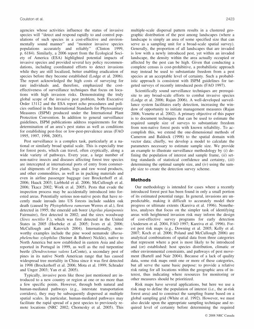
Fig. 3. The difference between PðS�2 jSþ1 Þ estimated using eq. 5 and the corresponding simulated value (estimated – simulated), by �2/A1 andA1/A2, in nine categories: (a) difference of £0.005; (b) difference of >0.005 and £0.01; (c) difference of >0.01 and £0.015; (d) the differenceof >0.015 and £0.02; (e) difference of >0.02 and £0.025; (f) difference of >0.025 and £0.03; (g) difference of >0.03 and £0.035; (h) differ-ence of >0.035 and £0.04; (i) difference of >0.04.

2426 Can. J. For. Res. Vol. 38, 2008

# 2008 NRC Canada

½7� P ¼ 1

�Xux¼l

N1�1

x

� �N1 � N1�1

n1 � x

� �N1

n1

� � ½ PðS�2 jSþ1 Þn2� �x�

0BB@

1CCA

We examined the difference between eq. 1 and eq. 7when calculating the probability of observing at least onepositive trap. To accomplish this, we set n1 = 1000 andused sequences of values for PðS�2 jSþ1 Þn2 (0.025, 0.05, . . .,0.975), �1n1 (5, 10, . . ., 25), and N1�1 (�1n1, �1n1 + 1, . . .,500). We calculated the sampling fraction for each combina-tion as �1n1/ N1�1. We computed N1 as n1 divided by thesampling fraction and rounded to the nearest integer. Thereason for calculating the variables as described was to forcerounding to the nearest integer to occur only on N1.

Results

Overall, estimates of PðS�2 jSþ1 Þ computed using eq. 5 werelarger than simulated estimates (Fig. 3). The mean differ-ence between the simulated and equation-based estimates

was 0.0166 with a root mean square error of 0.025. Thelargest difference, 0.19, was observed when A1/A2 = 50 andthe proportion of the stage-one sampling unit with the pestpresent was 0.5. The smallest difference, 0.000 05, was ob-served when A1/A2 = 4450 and the proportion of the stage-one sampling unit with the pest present was 0.025.Generally, the bias was larger when the trap was large com-pared with the area of the stage-one sampling unit (A1/A2)and when a large proportion of the stage-one sampling unitwas infested (�2/A1) (Fig. 3). When considering only thosesituations that are likely to occur when designing surveys atbroad spatial scales, the bias is <0.005 (Fig. 3a).

We examined differences in estimates of P between eq. 1and eq. 7 for several combinations of sampling fraction,PðS�2 jSþ1 Þ, and �1n1. Generally, the difference between thetwo estimates of P was <0.005 (Fig. 4). However, when thesampling fraction was, for instance, >0.3, PðS�2 jSþ1 Þ was setto a moderate value (e.g., 0.3–0.8), and �1n1 was small (e.g.,5), the difference between the estimates of P was >0.02(Fig. 4). Although the difference between the estimates of Pwas often small, these differences in P can have a substan-tial influence on n1 when the target precision of the surveyis high.

Fig. 4. The difference between eq. 1 and eq. 7 in the probability of observing at least one positive trap, by PðS�2 jSþ1 Þ and sampling fraction,for five different values of �1n1. Each row in the matrix is a different value of �1n1 and is labeled to the left of each row. Each columnrepresents a separate grouping of the difference, with the range for each group listed at the top of each column.

Coulston et al. 2427

# 2008 NRC Canada

Surveillance methodology exampleWhite et al. (1992) developed a global Environmental

Monitoring and Assessment (EMAP) sampling grid thatserves as the basis for the US Forest Service Forest Inven-tory and Analysis Phase 2 (forest mensuration) and Phase 3(forest health) surveys (Reams et al. 2005). The EMAP sam-pling grid was developed from a truncated icosahedronmade up of 20 hexagons and 12 pentagons covering theplanet, with one hexagon advantageously placed to coverNorth America (Fig. 5). A noteworthy aspect of the EMAPgrid’s configuration is that this hexagon can be systemati-cally intensified, yielding a wide range of potential sampleframes. This provides a straightforward framework for creat-ing a systematic, hexagonal survey lattice. In this case, eachhexagon created through intensification represents a stage-one sample unit that may be chosen.

Figure 5 displays a US risk map for a hypothetical non-native pest that attacks oaks (Quercus spp.). Suppose wewanted to design a survey to substantiate freedom from ourhypothetical pest outside its currently limited introduction

area. More specifically, we want to determine whether thepest exists in >5% of the stage-one sample units (�1 =0.05) at a within-unit prevalence (�2) of >50 km2, with90% certainty (P = 0.9). The effective area of our traps is1 km2 (A2); based on the risk map, there are approximately920 975 km2 of forest area at risk (RA). In practice, we useeq. 7 and vary n1 and n2 until the desired P is obtained.However, we must also have an estimate of N1 and A1 toapply eq. 7. For this example, we estimated these two vari-ables using an iterative approach applied to the risk map inFig. 5. The risk map was a raster spatial data layer whereeach cell was coded as either 0 = no risk or 1 = risk (out-side of the US boundary = null), and each cell was2.5 km � 2.5 km. We read the risk map into the R statisti-cal package (R Development Core Team 2006) as a matrixwith the same values and dimension as the geospatial data.RA was the product of the number of cells at risk and thecell size (6.25 km2). The total area (TA) was the product ofthe number of cells (disregarding null values) and the cellsize. For any value of n1, the total number of stage-one

Fig. 5. The North American hexagon from the EMAP sampling grid and areas of risk (shaded) for a hypothetical forest pest.

2428 Can. J. For. Res. Vol. 38, 2008

# 2008 NRC Canada

sample units that would cover the United States (NT) was cal-culated as TA � n1/RA. For simplicity, we considered each pri-mary sampling unit to be a square where the length of eachside (L), in units of number of cells from the original riskmap, was the number of rows in the original risk map dividedby N0:5

T . A1, in square kilometres, was then L2 � 6.25 km2 andN1 was the number of stage-one sampling units of size A1 thatcontained risk from the original map. We solved eq. 7 for n1 =100 to 1000 and n2 = 1 to 10, estimating N1 and A1 for eachvalue of n1, and selected the first n1 which achieved our goalof P = 0.9 for each value of n2.

To determine the optimal solution with respect to cost, weused a slightly modified version of eq. 3. The cost of travel-ing to a single stage-one sample unit to place (and eventu-ally retrieve) a trap was US$400 (Ca). The cost of the trapitself and of hiring an entomologist to examine its contentswas $200 (CT). The cost of adding a second trap to analready-sampled stage-one unit was $50 (CT2). The resultingcost function was

Ctotal ¼ Ca � n1 þ CT � n2 � n1 þ CT2ðn2 � 1Þn1The optimal solution was the values of n1 and n2 where thetotal cost was minimized. Based on our hypothetical costs,the optimal solution was n1 = 588 and n2 = 2, which had atotal cost of approximately US$499 800 (Table 1).

We followed the procedures outlined in Coulston et al.(2008) to develop a survey grid based on sampling n1 stage-one units. The first step was to estimate the intensificationfactor for the North American hexagon required to meet ourobjective of surveying 588 (hexagonal) units. We used theequation given by Coulston et al. (2008):

½8� X ¼ 5783883n1

RA

� �¼ 5783883� 588� 920975�1

¼ 3693

where X is the estimated intensification factor for the NorthAmerican hexagon and 5 783 833 is the coefficient from anonlinear regression model that relates the estimated sampleunit size to intensification factor.

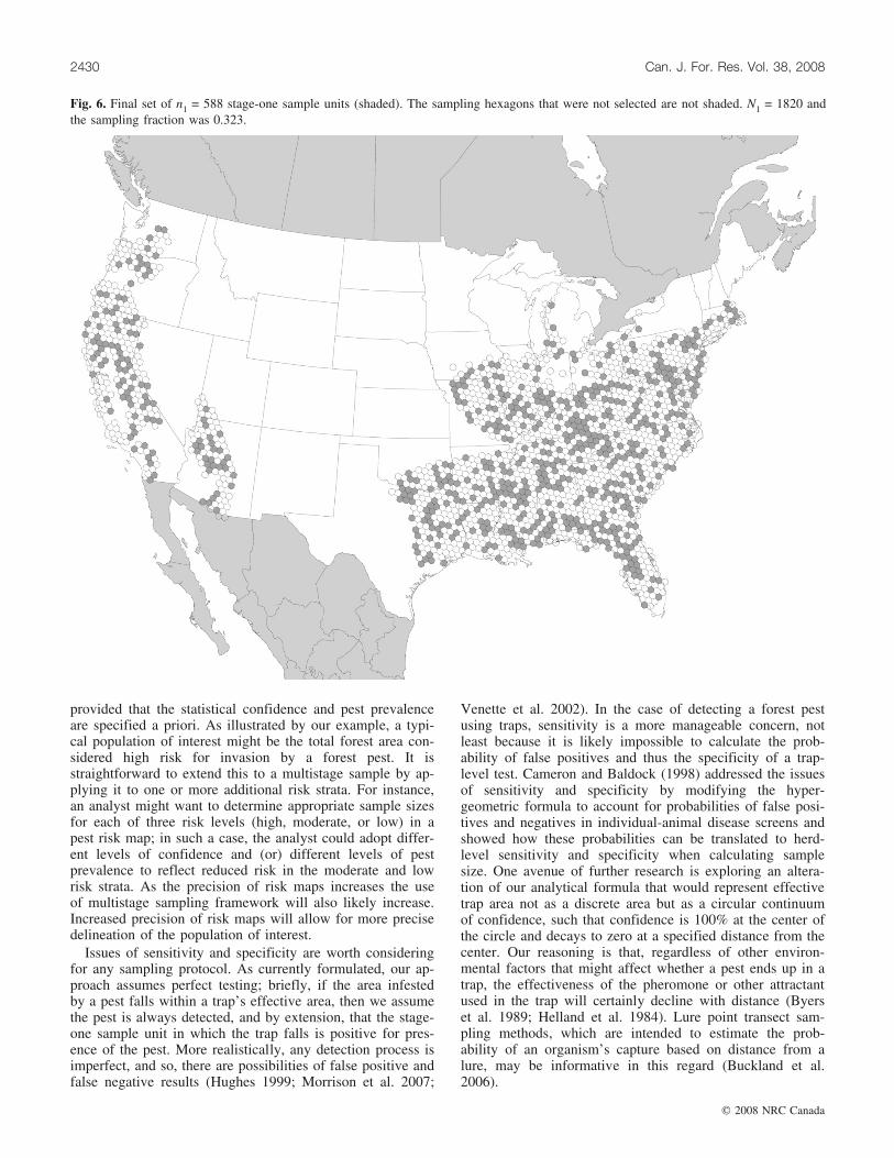
The geometric properties of the North American hexa-gon and its underlying triangular grid permit it to besystematically intensified by three, four, seven, or any fac-tor sequence combining these numbers (White et al. 1992).Therefore, for computational purposes, the estimatedintensification factor X must be rounded to the closestproduct of an eligible factor sequence. The closest possibleproduct (and sequence) to our target X = 3693 was 3888(3 � 3 � 3 � 3 � 3 � 4 � 4). Because risk maps gen-erally have moderate to low spatial and thematic accuracy,we considered each hexagon that contains any risk to becompletely at risk. Selecting all hexagons at risk yieldedN1 = 1820 total stage one sampling units. From this set,n1 = 588 sampling units were selected randomly (Fig. 6).The value of Al was 1536.8 km2. We verified the powerof our sample design using eq. 7; the probability of detect-ing at least one positive trap was 0.916.

Discussion

Our chief objective was to develop a practical method fordetermining an appropriate sample size to substantiate free-dom, at a specified level of confidence, from an invasiveforest pest using a global sampling grid. Depending on thepattern of risk observed from a risk map, it may be appro-priate to treat the stage-one sample as being drawn from aninfinite population. However, we suggest that, if the stage-one sampling fraction is high or the desired precision ishigh, then eq. 7 should be used. Regarding the stage-twoportion of the sample size equation, the equations presentedby Cameron and Baldock (1998) for sampling animals inlivestock herds may be straightforwardly translated to sam-pling trees in forested landscapes for forest diseases andsome insect pests (see also Hall et al. 2005, 2007; Venetteet al. 2002). However, in the case of certain mobile pests, asampling approach based on discrete, count-based variablesdoes not translate directly because the sample is an area(e.g., the effective area of a trap) rather than a number ofindividuals. As a result, it is necessary to extend the existingapproaches to two dimensions. We have shown an analyticalmethod (eq. 5) that applies for most broad spatial scale sce-narios in which these techniques would be relevant; how-ever, there are two scenarios where eq. 5 is not appropriate.This occurs when the ratio of the stage-one sample unit areato trap effective area (i.e., the stage-two sample unit area) isvery low and when the infested proportion of a stage-onesample unit is high (Fig. 3). Regarding the second scenario,it is unlikely that one would still be trying to establish free-dom from a pest if a large proportion of forested land hasalready been invaded by the pest. Anecdotal evidence of thepest’s presence is likely to be substantial at that point. Re-garding the first scenario, for most broad-scale surveys, thestage-one sample unit area will be much larger than the trapeffective area so this situation is not particularly relevant fornational-scale surveys. However, if either of the scenariosdescribed above are applicable, a simulation approachshould be used to estimate PðS�2 jSþ1 Þ.

We have described a two-stage sampling approach thatuses the relationship between (i) the number and area ofstage-one sample units and (ii) the effective trap area to de-termine the optimum sample size for a given spatial domain,

Table 1. Results from hypotheticalexample.

n1 n2 P Ctotal ($)859 1 0.900 515 400588 2 0.908 499 800484 3 0.900 532 400421 4 0.906 568 350381 5 0.911 609 600346 6 0.908 640 100317 7 0.900 665 700303 8 0.900 712 050290 9 0.915 754 000271 10 0.900 772 350

Note: Power is based on eq. 7 andusing eq. 5 to estimate PðS�2 jSþ1 Þ withn1 primary sampling units and n2

traps per primary sampling unit.Total cost (Ctotal) was minimizedwith n1 = 588 and n2 = 2.

Coulston et al. 2429

# 2008 NRC Canada

provided that the statistical confidence and pest prevalenceare specified a priori. As illustrated by our example, a typi-cal population of interest might be the total forest area con-sidered high risk for invasion by a forest pest. It isstraightforward to extend this to a multistage sample by ap-plying it to one or more additional risk strata. For instance,an analyst might want to determine appropriate sample sizesfor each of three risk levels (high, moderate, or low) in apest risk map; in such a case, the analyst could adopt differ-ent levels of confidence and (or) different levels of pestprevalence to reflect reduced risk in the moderate and lowrisk strata. As the precision of risk maps increases the useof multistage sampling framework will also likely increase.Increased precision of risk maps will allow for more precisedelineation of the population of interest.

Issues of sensitivity and specificity are worth consideringfor any sampling protocol. As currently formulated, our ap-proach assumes perfect testing; briefly, if the area infestedby a pest falls within a trap’s effective area, then we assumethe pest is always detected, and by extension, that the stage-one sample unit in which the trap falls is positive for pres-ence of the pest. More realistically, any detection process isimperfect, and so, there are possibilities of false positive andfalse negative results (Hughes 1999; Morrison et al. 2007;

Venette et al. 2002). In the case of detecting a forest pestusing traps, sensitivity is a more manageable concern, notleast because it is likely impossible to calculate the prob-ability of false positives and thus the specificity of a trap-level test. Cameron and Baldock (1998) addressed the issuesof sensitivity and specificity by modifying the hyper-geometric formula to account for probabilities of false posi-tives and negatives in individual-animal disease screens andshowed how these probabilities can be translated to herd-level sensitivity and specificity when calculating samplesize. One avenue of further research is exploring an altera-tion of our analytical formula that would represent effectivetrap area not as a discrete area but as a circular continuumof confidence, such that confidence is 100% at the center ofthe circle and decays to zero at a specified distance from thecenter. Our reasoning is that, regardless of other environ-mental factors that might affect whether a pest ends up in atrap, the effectiveness of the pheromone or other attractantused in the trap will certainly decline with distance (Byerset al. 1989; Helland et al. 1984). Lure point transect sam-pling methods, which are intended to estimate the prob-ability of an organism’s capture based on distance from alure, may be informative in this regard (Buckland et al.2006).

Fig. 6. Final set of n1 = 588 stage-one sample units (shaded). The sampling hexagons that were not selected are not shaded. N1 = 1820 andthe sampling fraction was 0.323.

2430 Can. J. For. Res. Vol. 38, 2008

# 2008 NRC Canada

The approach presented here adopts a key simplifying as-sumption with respect to spatial pattern: that the infestedarea in a given stage-one unit can be appropriately repre-sented as a single circle. A circle is the most compact of allpolygons in terms of perimeter/area ratio, but a pest is likelyto infest a potentially complex and irregularly shaped patchof the stage-one unit or, perhaps, multiple disconnectedpatches. As pattern complexity increases, the perimeter/arearatio also increases. When the perimeter/area ratio increases,the amount of additional area that must be accounted forbcecause of the trap area also increases, and the probabilityof failing to detect the pest’s presence decreases. In otherwords, the more complex is the pattern (and, thus, the higherthe perimeter/area ratio) exhibited by an infestation in agiven landscape, the more likely that a trap randomly placedon that landscape will intersect the infested area. Our circle-based approach gives a conservative estimate for the numberof samples necessary to demonstrate freedom from a forestpest. However, a second avenue of future research is to ex-tend our analytical formula to incorporate more complex in-festation patterns and thus improve both realism andperformance.

Our explanation operates largely from the perspective thata user, when calculating sample size, is focused on achiev-ing a desired level of confidence given certain pest preva-lence levels within and among forested landscapes.Nonetheless, as Cameron and Baldock (1998) suggest, ifprevalence levels are low but the desired confidence ishigh, a large sample size and potentially expensive surveymay result. This emphasizes the utility of a cost functionthat incorporates expenses such as trap placement as well asanalysis of the trap contents through time in determining anoptimal solution. However in some situations, the budgetwill be the limiting factor, i.e., the user will know howmany samples or traps he or she can afford to place andanalyze. In such cases, it is possible to back-calculate usingour formulae to establish the detection power given the af-fordable sample size.

An overall aim of this research was development of meth-ods, including optimum sample size determination, to gener-ate broad spatial scale (e.g., national-scale) survey schemesfor substantiating freedom for invasive forest pests. Our pro-posed approach is consistent with ISPM guidelines for tar-geted pest surveys (Food and Agriculture Organization1995, 1998) and also addresses the recommendation ofLodge et al. (2006) to ‘‘use new technology to improve ac-tive surveillance of invasive species to increase the successof rapid response and eradication efforts’’ (p. 2045). Indeed,the techniques we employ provide tools for pest managers toconstruct surveys rapidly once a risk map has been created.Although other probabilistic methodologies for determiningpest-free status have been proposed (e.g., Barclay andHargrove 2005), our risk map based approach has the furtheradvantage of translating directly into a spatially referenced,cost-effective pest surveillance strategy (Regan et al. 2006).Lodge et al. (2006) also recommended the development ofmore quantitative approaches to risk analysis. We supporttheir recommendation and expect the cost-efficiency of sur-vey grids to substantiate freedom from an invasive pest toincrease with improvement in risk analysis and risk map-ping. Our hypothetical pest example demonstrates how,

once the sample size is determined, it is possible to use thisnumber to intensify the EMAP hexagon for North Americaand generate a wall-to-wall tessellation of sampling poly-gons for the conterminous United States (see also Coulstonet al. 2008). With respect to sampling other countries or re-gions, any of the 19 other hexagonal faces in the EMAPsampling grid may be intensified in a similar manner; someregularity would be lost when intensifying one of the 12pentagonal faces, but it is relatively straightforward to shiftthe grid and optimally place a hexagon over any target areaof interest (White et al. 1992).

Finally, the USDA Forest Service, in cooperation withother agencies, has recently produced national-scale riskmaps for non-native forest pests that have been regularly de-tected at ports of entry yet never found to be introduced be-yond port facilities. This sort of ‘‘preemptive’’ risk analysishas also been completed for pests threatening Europe, NewZealand, and other parts of the globe (e.g., MacLeod et al.2002; Pitt et al. 2007). Such risk maps may also function asinputs for our sampling method, giving forest health manag-ers a simple way to allocate resources for best determiningthe current status of these pests within their country or re-gion of interest.

AcknowledgementsThis research was supported in part through Research

Joint Venture Agreement 07-JV-11330146-135 between theUSDA Forest Service, Southern Research Station, Asheville,North Carolina, and North Carolina State University. Wethank the two anonymous reviewers for comments and sug-gestions on this manuscript. We also thank the associate ed-itor for insightful comments and help in utilizing thehypergeometric distribution.

ReferencesAndersen, M.C., Adams, H., Hope, B., and Powell, M. 2004. Risk

assessment for invasive species. Risk Anal. 24: 787–793. doi:10.1111/j.0272-4332.2004.00478.x. PMID:15357799.

Barclay, H.J., and Hargrove, J.W. 2005. Probability models to fa-cilitate a declaration of pest-free status, with special referenceto tsetse (Diptera: Glossinidae). Bull. Entomol. Res. 95: 1–11.doi:10.1079/BER2004331. PMID:15705209.

Bartell, S.M., and Nair, S.K. 2004. Establishment risks for invasivespecies. Risk Anal. 24: 833–845. doi:10.1111/j.0272-4332.2004.00482.x. PMID:15357803.

Brockerhoff, E.G., Bain, J., Kimberley, M., and Knızek, M.. 2006.Interception frequency of exotic bark and ambrosia beetles (Co-leoptera: Scolytinae) and relationship with establishment in NewZealand and worldwide. Can. J. For. Res. 36: 289–298. doi:10.1139/x05-250.

Buckland, S.T., Summers, R.W., Borchers, D.L., and Thomas, L.2006. Point transect sampling with traps and lures. J. Appl.Ecol. 43: 377–384. doi:10.1111/j.1365-2664.2006.01135.x.

Byers, J.A., Anderbrant, O., and Lofqvist, J. 1989. Effectiveattraction radius: a method for comparing species attractantsand determining densities of flying insects. J. Chem. Ecol. 15:749–765. doi:10.1007/BF01014716.

Cameron, A.R., and Baldock, F.C. 1998. Two-stage sampling in sur-veys to substantiate freedom from disease. Prev. Vet. Med. 34:19–30. doi:10.1016/S0167-5877(97)00073-1. PMID:9541948.

Cannon, R.M., and Roe, R.T. 1982. Livestock disease surveys. Amanual for veterinarians. Bureau of Rural Science, Department

Coulston et al. 2431

# 2008 NRC Canada

of Primary Industry, Australian Government Publishing Service,Canberra, Aust.

Chornesky, E.A., Bartuska, A.M., Aplet, G.H., Britton, K.O.,Cummings-Carlson, J., Davis, F.W., Eskow, J., Gordon, D.R.,Gottschalk, K.W., Haack, R.A., Hansen, A.J., Mack, R.N.,Rahel, F.J., Shannon, M.A., Wainger, L.A., and Wigley, T.B.2005. Science priorities for reducing the threat of invasive spe-cies to sustainable forestry. Bioscience, 55: 335–348. doi:10.1641/0006-3568(2005)055[0335:SPFRTT]2.0.CO;2.

Clark, R.G., and Steel, D.G. 2000. Optimum allocation of sampleto strata and stages with simple additional constraints. Statisti-cian, 49: 197–207. doi:10.2307/2680969.

Clinton, W.J. 1999. Executive Order 13112 of February 3, 1999:invasive species. Fed. Regist. 64: 6183–6186.

Cochran, W.G. 1977. Sampling techniques. 3rd ed. Wiley, NewYork.

Coulston, J.W., Koch, F.H., Smith, W.D., and Sapio, F.J. 2008. De-veloping survey grids to substantiate freedom from exotic pests.In Proceedings of the 8th Annual Forest Inventory and Analysis(FIA) Symposium, 16–19 Oct. 2006, Monterey, Calif. USDAFor. Serv. Gen. Tech. Rep. WO-xx. In press.

Downing, M.C., Borchert, D.M., Duerr, D.A., Haugen, D.A., Koch,F.H., Krist, F.J., Sapio, F.J., Smith, W.D., and Tkacz, B.M.2005. National risk maps for the sirex woodwasp (Sirex noctilio)[online]. USDA Forest Service, Forest Health Technology Enter-prise Team, Fort Collins, Colo. Available from http://www.fs.fed.us/foresthealth/technology/invasives_sirexnoctilio_riskmaps.shtml [accessed 15 October 2007].

Ellison, A.M., Bank, M.S., Clinton, B.D., Colburn, E.A., Elliott,K., Ford, C.R., Foster, D.R., Kloeppel, B.D., Knoepp, J.D.,Lovett, G.M., Mohan, J., Orwig, D.A., Rodenhouse, N.L.,Sobczak, W.V., Stinson, K.A., Stone, J.K., Swan, C.M.,Thompson, J., Von Holle, B., and Webster, J.R. 2005. Loss offoundation species: consequences for the structure and dynamicsof forested ecosystems. Front. Ecol. Environ, 3: 479–486.doi:10.1890/1540-9295(2005)003[0479:LOFSCF]2.0.CO;2.

Food and Agriculture Organization (FAO). 1995. Requirements forthe establishment of pest free areas. International Standards forPhytosanitary Measures, Secretariat of the International PlantProtection Convention, U.N. Food and Agriculture Organization,Rome. Publ. 4.

Food and Agriculture Organization (FAO). 1997. Guidelines forsurveillance. International Standards for Phytosanitary Measures,Secretariat of the International Plant Protection Convention,U.N. Food and Agriculture Organization, Rome. Publ. 6.

Food and Agriculture Organization (FAO). 1998. Determination ofpest status in an area. International Standards for PhytosanitaryMeasures, Secretariat of the International Plant Protection Con-vention, United Nations Food and Agriculture Organization,Rome. Publ. 8.

Food and Agriculture Organization (FAO). 2005. Requirements forthe establishment of areas of low pest prevalence. InternationalStandards for Phytosanitary Measures, Secretariat of the Interna-tional Plant Protection Convention, United Nations Food andAgriculture Organization, Rome. Publ. 22.

Haack, R.A. 2001. Intercepted Scolytidae (Coleoptera) at U.S. portsof entry: 1985–2000. Integr. Pest Manage. Rev. 6: 253–282.doi:10.1023/A:1025715200538.

Hall, D.G., Childers, C.C., and Eger, J.E. 2005. Effects of reducingsample size on density estimates of citrus rust mite (Acari: Erio-phyidae) on citrus fruit: simulated sampling. J. Econ. Entomol.98: 1048–1057. PMID:16022338.

Hall, D.G., Childers, C.C., and Eger, J.E. 2007. Binomial samplingto estimate rust mite (Acari: Eriophyidae) densities on orange

fruit. J. Econ. Entomol. 100: 233–240. doi:10.1603/0022-0493(2007)100[233:BSTERM]2.0.CO;2. PMID:17370833.

Helland, I.S., Hoff, J.M., and Anderbrant, O. 1984. Attraction ofbark beetles (Coleoptera: Scolytidae) to a pheromone trap. J.Chem. Ecol. 10: 723–752. doi:10.1007/BF00988539.

Hoebeke, E.R., Haugen, D.A., and Haack, R.A. 2005. Sirex nocti-lio: discovery of a palearctic siricid woodwasp in New York.Newsl. Mich. Entomol. Soc. 50: 24–25.

Hughes, G. 1999. Sampling for decision making in crop loss as-sessment and pest management: introduction. Phytopathology,89: 1080–1083. doi:10.1094/PHYTO.1999.89.11.1080.

Ivors, K., Garbelotto, M., Vries, D.E., Rutyer-Spira, C., Hekkert,B.T., Rosenzweig, N., and Bonants, P. 2006. Microsatellite mar-kers identify three lineages of Phytophthora ramorum in USnurseries, yet single lineages in US forest and European nurserypopulations. Mol. Ecol. 15: 1493–1505. doi:10.1111/j.1365-294X.2006.02864.x. PMID:16629806.

Kareiva, P., Parker, I.M., and Pascual, M. 1996. Can we use ex-periments and models in predicting the invasiveness of geneti-cally engineered organisms? Ecology, 77: 1670–1675. doi:10.2307/2265771.

Kelly, M., Guo, Q., Liu, D., and Shaari, D. 2007. Modeling the riskfor a new invasive forest disease in the United States: an evalua-tion of five environmental niche models. Comput. Environ. UrbanSyst. 31: 689–710. doi:10.1016/j.compenvurbsys.2006.10.002.

Koch, F.H., Cheshire, H.M., and Devine, H.A. 2006. Landscape-scale prediction of hemlock woolly adelgid, Adelges tsugae(Homoptera: Adelgidae), infestation in the southern AppalachianMountains. Environ. Entomol. 35: 1313–1323. doi:10.1603/0046-225X(2006)35[1313:LPOHWA]2.0.CO;2.

Liebhold, A.M., Work, T.T., McCullough, D.G., and Cavey, J.F.2006. Airline baggage as a pathway for alien insect species in-vading the United States. Am. Entomol. 52: 48–54.

Lodge, D.M., Williams, S., MacIsaac, H.J., Hayes, K.R., Leung, B.,Reichard, S., Mack, R.N., Moyle, P.B., Smith, M., Andow,D.A., Carlton, J.T., and McMichael, A. 2006. Biologicalinvasions: recommendations for U.S. policy and management.Ecol. Appl. 16: 2035–2054. doi:10.1890/1051-0761(2006)016[2035:BIRFUP]2.0.CO;2. PMID:17205888.

MacLeod, A., Evans, H.F., and Baker, R.H.A. 2002. An analysis ofpest risk from an Asian longhorn beetle (Anoplophora glabri-pennis) to hardwood trees in the European community. CropProt. 21: 635–645. doi:10.1016/S0261-2194(02)00016-9.

McCullough, D.G., and Katovich, S.A. 2004. Pest alert: emeraldash borer [online]. USDA Forest Service, State and Private For-estry, Northeastern Area, Newton Square, Pa. Publ. NA-PR-02-04. Available from http://na.fs.fed.us/spfo/pubs/pest_al/eab/eab04.htm [accessed 15 October 2007].

McCullough, D.G., Work, T.T., Cavey, J.F., Liebhold, A.M., andMarshall, D. 2006. Interceptions of nonindigenous plant pestsat US ports of entry and border crossings over a 17-yearperiod. Biol. Invasions, 8: 611–630. doi:10.1007/s10530-005-1798-4.

McDougall, K.L., St, J., Hardy, G.E., and Hobbs, R.J. 2002. Distri-bution of Phytophthora cinnamomi in the northern jarrah (Euca-lyptus marginata) forest of Western Australia in relation todieback age and topography. Aust. J. Bot. 50: 107–114. doi:10.1071/BT01040.

Morrison, S.A., MacDonald, N., Walker, K., and Shaw, M.R. 2007.Facing the dilemma at eradication’s end: uncertainty of absenceand the Lazarus effect. Front. Ecol. Environ. 5: 271–276. doi:10.1890/1540-9295(2007)5[271:FTDAEE]2.0.CO;2.

Mota, M.M., Braasch, H., Bravo, M.A., Penas, A.C.,Burgermeister, W., Metge, K., and Sousa, E. 1999. First report

2432 Can. J. For. Res. Vol. 38, 2008

# 2008 NRC Canada

of Bursaphelenchus xylophilus in Portugal and in Europe. Ne-matology, 1: 727–734. doi:10.1163/156854199508757.

National Research Council (NRC), Committee on the ScientificBasis for Predicting the Invasive Potential of NonindigenousPlants and Plant Pests in the United States, Board on Agricultureand Natural Resources. 2002. Predicting invasions of non-indigenous plants and plant pests. National Academy Press, Wa-shington, D.C.

Pimentel, D., Zuniga, R., and Morrison, D. 2005. Update on the en-vironmental and economic costs associated with alien-invasivespecies in the United States. Ecol. Econ. 52: 273–288. doi:10.1016/j.ecolecon.2004.10.002.

Pitt, J.P.W., Regniere, J., and Worner, S. 2007. Risk assessment ofthe gypsy moth, Lymantria dispar (L), in New Zealand based onphenology modeling. Int. J. Biometeorol. 51: 295–305. doi:10.1007/s00484-006-0066-3. PMID:17120064.

Poland, T.M., and McCullough, D.G. 2006. Emerald ash borer: in-vasion of the urban forest and the threat to North America’s ashresource. J. For. 104: 118–124.

R Development Core Team. 2006. R: a language and environmentfor statistical computing. R Foundation for Statistical Compu-ting,Vienna, Austria.

Rajan. 2006. Surveillance and monitoring for plant parasitic nema-todes—a challenge. EPPO Bull. 36: 59–64. doi:10.1111/j.1365-2338.2006.00942.x.

Reams, G.A., Smith, W.D., Hansen, M.H., Bechtold, W.A.,Roesch, F.A., and Moisen, G.G. 2005. The Forest Inventory andAnalysis sampling frame. In The enhanced Forest Inventory andAnalysis Program—national sampling design and estimationprocedures. Edited by W.A. Bechtold and P.L. Patterson. USDAFor. Serv. Gen. Tech. Rep. SRS-80. pp. 11–26.

Regan, T.J., McCarthy, M.A., Baxter, P.W.J., Panetta, F.D., andPossingham, H.P. 2006. Optimal eradication: when to stop look-

ing for an invasive plant. Ecol. Lett. 9: 759–766. doi:10.1111/j.1461-0248.2006.00920.x. PMID:16796564.

Reilly, M. 1996. Optimal sampling strategies for two-stage studies.Am. J. Epidemiol. 143: 92–100. PMID:8533752.

Schrader, G., and Unger, J.G. 2003. Plant quarantine as a measureagainst invasive alien species: the framework of the Interna-tional Plant Protection Convention and the plant health regula-tions in the European Union. Biol. Invasions, 5: 357–364.doi:10.1023/B:BINV.0000005567.58234.b9.

Tkacz, B.M. 2002. Pest risks associated with importing wood to theUnited States. Can. J. Plant Pathol. 24: 111–116.

Venette, R.C., Moon, R.D., and Hutchison, W.D. 2002. Strategiesand statistics of sampling for rare individuals. Annu. Rev. Ento-mol. 47: 143–174. doi:10.1146/annurev.ento.47.091201.145147.PMID:11729072.

Waters, J.R., and Chester, A.J. 1987. Optimal allocation in multi-variate, two-stage sampling designs. Am. Stat. 41: 46–50.doi:10.2307/2684319.

White, D., Kimerling, J.A., and Overton, S.W. 1992. Cartographicand geometric components of a global sampling design for en-vironmental monitoring. Cartogr. Geogr. Inf. Sci. 19: 5–22.doi:10.1559/152304092783786636.

Wilcove, D.S., Rothstein, D., Dubow, J., Phillips, A., and Losos, E.1998. Quantifying threats to imperiled species in the UnitedStates. Bioscience, 48: 607–615. doi:10.2307/1313420.

Work, T.T., McCullough, D.G., Cavey, J.F., and Komsa, R. 2005.Arrival rate of nonindigenous insect species into the UnitedStates through foreign trade. Biol. Invasions, 7: 323–332.doi:10.1007/s10530-004-1663-x.

Yan, Z., Sun, J., Don, O., and Zhang, Z. 2005. The red turpentinebeetle, Dendroctonus valens LeConte (Scolytidae): an exotic in-vasive pest of pine in China. Biodivers. Conserv. 14: 1735–1760.doi:10.1007/s10531-004-0697-9.

Coulston et al. 2433

# 2008 NRC Canada