Embed Size (px)
Citation preview
Proceedings of Symposia in Pure Mathematics
Invariant Measures for actions of Higher
Rank Abelian groups
Boris Kalinin 1) and Anatole Katok 2)
Abstract. The first part of the paper begins with an introductioninto Anosov actions of Zk and Rk and an overview of the methodof studying invariant measures for such actions based on consid-eration of conditional measures along various invariant foliations.The main body of that part contains a detailed proof of a modi-fied version of the main theorem from [KS3] for actions by toralautomorphisms of with applications to rigidity of the measurablestructure of such actions with respect to Lebesque measure. In thesecond part principal technical tools for studying nonuniformly hy-perbolic actions of Zk and Rk are introduced and developed. Theseinclude Lyapunov characteristic exponents, nonstationary normalforms and Lyapunov Hoelder structures. At the end new rigidityresults for Z2 actions on three-dimensional manifolds are outlined.
In this paper we discuss various results concerning invariant mea-sures for actions of higher–rank abelian groups, i.e. Zk and Rk fork ≥ 2 on compact differentiable manifolds which display certain hy-perbolic behavior. Similarly to the rank one case, hyperbolicity can befull or partial, and uniform or nonuniform. Full (corr. partial) uniformhyperbolicity appears for Anosov (corr. partially hyperbolic) actions.Nonuniform hyperbolicity appears for actions preserving measures forwhich all (for the full case) or some (for partial case) Lyapunov char-acteristic exponents do not vanish. Two parts of the paper deals withthe uniform and nonuniform cases correspondingly.
While the final text of this paper is the product of a joint effort thebasic drafts of various parts were written separartely: that for Section3 was written by B. Kalinin and based on a part of his Ph. D thesis;for the rest of the paper the draft was written by A. Katok.
1) This work has been partially supported by NSF grant DMS-9704776.2) Partially supported by NSF grants DMS-9704776 and DMS-0071339.
1

2 BORIS KALININ AND ANATOLE KATOK
We would like to thank Ralf Spatzier for carefully reading the paperand making a number of valuable suggestions and corrections.
Part I. UNIFORMLY HYPERBOLIC ACTIONS
1. Definitions and examples
1.1. Anosov and partially hyperbolic actions.
1.1.1. Anosov actions of discrete and continuous groups. A smoothaction α of a discrete group Γ on a compact manifoldM is called Anosovif for some γ ∈ Γ, α(γ) is an Anosov diffeomorphism, i.e. the tangentbundle TM splits in an α(γ) invariant way into two subbundles (dis-tributions) E− and E+ called the stable (or contracting) and unstable(or expanding) bundles (or distributions) correspondingly such that forsome λ, 0 < λ < 1 and C ≥ 1 and for all positive integers m,
(1.1.1) ‖D(α(γm))(v)‖ ≤ Cλm.
if v ∈ E− and
(1.1.2) ‖D(α(γm))(v)‖ ≥ C−1λ−m.
if v ∈ E+
Here ‖ · ‖ is the norm in TM generated by a Riemannian metric onM and D is the derivative map. The constant C (but not λ) dependson the choice of Riemannian metric.
More generally, a smooth locally free action of a Lie group G iscalled Anosov (or normally hyperbolic) if for a certain element condi-tions (1.1.1) and (1.1.2) hold for E− and E+ in the splitting TM =Eo ⊕ E− ⊕ E+, where Eo is the tangent bundle to the orbit foliationof the action. See [KS1] for a more detailed discussion. Such an ele-ment γ is then called normally hyperbolic. In this case the distributionsE− and E+ are often called the strong stable and the strong unstabledistributions.
The general theory of Anosov actions even for higher–rank abeliangroups is not well developed. The first serious obstruction is the fol-lowing open question.
Problem. For an Anosov action of Rk, k ≥ 2 is the set N of normallyhyperbolic elements dense?
A similar question for Zk actions is reduced to this one via suspen-sion construction (Section 1.2.2). The set N is open and its connectedcomponents are convex cones. In all known examples Rk \ N is theunion of finitely many hyperplanes (cf. Lyapunov hyperplanes, Sec-tions 1.2.3, 1.3, 5.2).

INVARIANT MEASURES FOR ACTIONS OF ABELIAN GROUPS 3
1.1.2. Partially hyperbolic actions. A more general class is formedby partially hyperbolic actions. A G action α is called partially hy-perbolic if there is an γ ∈ G and a α(γ)–invariant splitting TM =E−⊕E+⊕E0, with E− and E+ satisfying (1.1.1) and (1.1.2) as beforeand E0 the “slow” distribution with
(1.1.3) (C ′)−1µ−m ≥ ‖D(α(γm))(v)‖ ≤ C ′µm
for some µ, λ < µ ≤ 1 and C ′ ≥ 11.1.3. Contrast between rank one and higher rank. Any discussion
of Anosov actions of higher rank abelian groups requires a certain con-dition of being “genuinely higher rank” in order to avoid products ofrank one actions and other situations which can be reduced to the rankone case. The structure of such actions in the higher–rank case looksquite different and much more rigid than in the classical rank one situ-ation of diffeomorphisms (Z–actions) and flows (R-actions). All knownexamples of such actions satisfying the “genuine higher rank” assump-tions are algebraic up to a differentiable conjugacy. In particular, mostalgebraic actions are known to be differentiably rigid [KS2]. For thealgebraic actions a natural condition is absence of rank one algebraicfactors. (See e.g. Section 3.1, condition (R′)). Thus studying invariantmeasures for irreducible algebraic Anosov (and in certain cases, alsopartially hyperbolic) actions is quite natural.
One of the main differences between the rank one and higher ranksituations may be highlighted as follows. In the former case the robustorbit structure is well–described by the Markov model via a Markovpartition (see, e.g. [KH], Section 18.7). In particular, any invariantmeasure for the topological Markov chain associated with a Markovpartition produces an invariant measure for the hyperbolic system inquestion. The variety of invariant measures, both well–structured andnot, for a topological Markov chain, is huge; hence the same is truefor the hyperbolic systems. In the higher–rank case the Markov modelis not applicable, since natural topological Markov chains consist ofmaps with infinite topological entropy. Hence algebraic models shouldbe understood more directly.
1.2. Higher Rank Actions by Toral Automorphisms. Themost basic examples of smooth hyperbolic actions of higher rank abeliangroups are actions by automorphisms of a torus and their suspensions.
1.2.1. Preliminaries. Denote by GL(m,Z) the group of integralm×m matrices with determinant 1 or −1. Any matrix A ∈ GL(m,Z)

4 BORIS KALININ AND ANATOLE KATOK
defines an automorphism of the torus Tm = Rm/Zm which we denoteby FA.
The automorphism FA is ergodic with respect to Lebesgue measureon Tm if and only if no eigenvalue of A is a root of unity.
This can be seen by considering the dual automorphism on thegroup of characters Zm. If A (and hence the transposed matrix At) hasan r th root of unity as an eigenvalue there is a rational (and hence alsoan integer) invariant vector for (At)r. Hence the operator UF r
Ainduced
by (FA)r on L2, has a nonconstant invariant function, the correspondingcharacter χ, and
∑r−1i=0 χ ◦ (F i
A) is an invariant nonconstant functionfor UFA
.On the other hand, if there are no roots of unity among the eigen-
values, all orbits of At acting on the characters, save the constants, areinfinite and hence the operator UF r
Ahas countable Lebesgue spectrum
in the orthogonal complement to the constant and thus FA is ergodic.Furthermore, in the latter case A has an eigenvalue of absolute value
greater then one (this can be seen by using a bit of linear algebra anda compactness argument), and FA is a Bernoulli automorphism withrespect to Lebesgue measure [Kat].
Any Zk action α by automorphisms of Tm is given by an embeddingρα : Zk → GL(m,Z) such that α(n) = Fρα(n), where n = (n1, ..., nk) ∈Zk.
Let α1 and α2 be two Zk actions by automorphisms of Tm1 andTm2 correspondingly. The action α2 is called an algebraic factor of a1
if there exists an epimorphism h: Tm1 → Tm2 such that h◦α1 = α2 ◦h.The action α is called irreducible if any algebraic factor has finite
fibers, i.e. acts on the torus of the same dimension. Equivalently, αdoes not have any invariant subtorus of lower dimension, or ρα containsa matrix with irreducible characteristic polynomial [B]. In [KS3, KS4]irreducible actions are called completely irreducible.
1.2.2. Suspension construction. It will be more convenient for usto operate with Rk actions so we would like to pass from an action ofZk to the corresponding action of Rk. This is the so-called suspensionconstruction.
Suppose Zk acts on Tm. Embed Zk as a lattice in Rk. Given a Zk
action α on the torus let Zk act on Rk × Tm by
(1.2.1) α(n)(t, x) = (t− n, α(n)(x))
and form the quotient
(1.2.2) M = Rk × Tm/Zk.

INVARIANT MEASURES FOR ACTIONS OF ABELIAN GROUPS 5
Note that the “vertical” action V of Rk on Rk × Tm by Vs(t, x) =(t + s, x) commutes with the Zk-action and therefore descends to M .This Rk-action is called the suspension of the Zk-action.
Note that any Zk-invariant measure on Tm lifts to a unique Rk-invariant measure on M .
The manifold M is a fibration over the ”time” torus Tk with thefiber Tm. We note that TM splits into the direct sum TM = TfM ⊕ToM where TfM is the subbundle tangent to the Tm fibers and ToMis the subbundle tangent to the orbit foliation.
Remark. The suspension construction is of very general nature. Namely,let α be an action of Zk on a space X with a certain structure (mea-sure, topology, differentiable, homogeneous, etc). Then (1.2.1) definesan action on the product and the factor (1.2.2) possesses the structureof the skew product over Tk with the fiber X and inherits the structurefrom the fiber. This structure is preserved by the suspension action ofRk.
1.2.3. Eigenvalues and Lyapunov Exponents. Let us denote by A1, ..., Ak
the generators of the action α, i.e. the images under ρα of the standardgenerators of Zk. For each Ai Rm splits as the direct sum of the rootspaces of Ai:
Rm =⊕
λ∈SpAi
Ker(Ai − λ)m.
Since the matrices Ai commute there exists an invariant splittingRm =
⊕Vj which is a common refinement of the above splittings.
It is called the root decomposition for the action α. It follows thatthe tangent bundle TTm = Tm × Rm splits into the direct sum of theinvariant subbundles corresponding to subspaces Vj. The Lyapunovexponent λ(α(n), v) exists for every element α(n) ∈ Gα and every vec-tor v ∈ TTm. If v lies in one of the subbundles then λ(α(n), v) equalsto the logarithm of the absolute value of the corresponding eigenvalueof element α(n). Moreover, λ(α(·), v) is an additive functional on Zk.Combining the subspaces Vj corresponding to the same Lyapunov ex-ponent we obtain a more robust decomposition than the root decompo-sition which is called the Lyapunov decomposition for the action α. Forthe detailed discussion of Lyapunov exponents for Zk and Rk actionsby automorphisms of tori and solenoids including the non-Archimedeanexponents appearing from p-adic valuations, see [KS3, Section 2 andAppendix]. We will return to the discussion of Lyapunov exponents ingreater generality, first for algebraic actions in Section 1.3, and then inthe general setting in Section 5.
6 BORIS KALININ AND ANATOLE KATOK
The Lyapunov exponent for the suspension corresponding to ToMis always identically zero. To exclude this trivial case, when we speakof Lyapunov exponents we will always mean the Lyapunov exponentscorresponding to TfM . These Lyapunov exponents of the Rk actionare the extensions of the Lyapunov exponents of the Zk action to thelinear functionals on Rk. The kernels of non-zero Lyapunov exponentsare called Lyapunov hyperplanes. Lyapunov exponents may be pro-portional to each other with positive or negative coefficients. In thiscase, they define the same Lyapunov hyperplane. The action is Anosov(Section 1.1) if there are no non-trivial identically zero Lyapunov ex-ponents.
Definition. The action α is called totally nonsymplectic (TNS) if noLyapunov exponents are proportional with a negative coefficient.
For a generalization of this concept see Section 5.2.An element a ∈ Rk is called regular if it does not belong to any
Lyapunov hyperplane. All other elements are called singular. We call asingular element generic if it belongs to only one Lyapunov hyperplane.A regular element for an Anosov action is called an Anosov element.
In the situation we are considering now, i.e for actions by auto-morphisms of the torus and for the suspensions of such actions, everyLyapunov subspace is uniquely integrable to a homogeneous foliation.This is not always the case for more general actions including homo-geneous ones (Section 1.3); the coarse Lyapunov decomposition whichcombines positively proportional Lyapunov exponents is always inte-grable (Section 5.2).
For an element a ∈ Rk let us define the stable, unstable and centerdistributions E−
a , E+a and E0
a as the sum of the Lyapunov spaces forwhich the value of the corresponding Lyapunov exponent on a is nega-tive, positive, and 0 respectively. For any singular element a the centerdistributions E0
a always contains an invariant subdistribution EIa , called
isometric distribution. For an element a we will denote the integral fo-liations of the stable, unstable, center and isometric distributions E−
a ,E+
a , E0a and EI
a by W−a , W+
a , W 0a and W I
a correspondingly.
1.3. General algebraic actions. Now we will consider “essen-tially algebraic” partially hyperbolic (in particular Anosov) actions ofeither Rk or Zk more general than actions by toral automorphisms andtheir suspensions.
We recall that an action of a group G on a compact manifold isAnosov if some element g ∈ G acts normally hyperbolically with respectto the orbit foliation (Section 1.1; see [KS1] for more details).

INVARIANT MEASURES FOR ACTIONS OF ABELIAN GROUPS 7
1.3.1. Affine actions of discrete groups. To clarify the notion of analgebraic action, let us first define affine algebraic actions of discretegroups. Let H be a connected Lie group with Λ ⊂ H a cocompactlattice. Define Aff(H) as the set of diffeomorphisms of H which mapright invariant vector-fields on H to right invariant vectorfields. DefineAff(H/Λ) to be the diffeomorphisms of H/Λ which lift to elementsof Aff(H). Finally, define an action ρ of a discrete group G on H/Λto be affine algebraic if ρ(g) is given by some homomorphism G →Aff(H/Λ). Let h be the Lie algebra of H . Identifying h with the rightinvariant vectorfields on H , any affine algebraic action determines ahomomorphism σ : G → Aut h. Call σ the linear part of this action.We will also allow quotient actions of these on finite quotients of H/Λ,e.g. on infranilmanifolds. For any Anosov algebraic action of a discretegroup G, H has to be nilpotent (cf. eg. [GS], Proposition 3.13).
1.3.2. Algebraic Rk-actions. . Suppose Rk ⊂ H is a subgroup ofa connected Lie group H . Let Rk act on a compact quotient H/Λ byleft translations where Λ is a lattice in H . Suppose C is a compactsubgroup of H which commutes with Rk. Then the Rk-action on H/Λdescends to an action on M = C \ H/Λ. The general algebraic Rk-action ρ is a finite factor of such an action. Let c be the Lie algebra ofC. The linear part of ρ is the representation of Rk on c \ h induced bythe adjoint representation of Rk on the Lie algebra h of H .
Let us note that the suspension (Section 1.2.2) of an algebraic Zk-action is an algebraic Rk-action (cf. [KS1], Section 2.2).
Let ρ be an algebraic action of Rk, not necessarily Anosov. Fora given a ∈ Rk we denote the strong stable foliation of ρ(a) by W−
a ,the strong stable distribution by E−
a , and the 0-Lyapunov space byE0
a. Note that E0a is always integrable for algebraic actions. Denote
the corresponding foliation by W0a . For a ρ–invariant Borel probability
measure µ let us denote by ξa the partition into ergodic components ofthe element ρ(a), by hµ(a) the measure–theoretic entropy of the mapρ(a) and by π(a) the π–partition of ρ(a). Recall that π(a) is in factequal to the measurable hull ξ(W−
a ) of the partition into the leaves ofthe strong stable foliation W−
a .1.3.3. Lyapunov exponenets. Let us describe the structure of the
linear part of an algebraic Rk actions in more detail. In fact, we willfirst consider the case on the actions on H/Λ. The Lie algebra h splitsinto root spaces hα, α ∈ Σ of the adjoint representation. The roots arelinear functionals on Rk and their real parts in fact coincide with theLyapunov exponents of the action ρ. The positive half–space ℜα ≥ 0is called a Lyapunov half–space and its boundary a Lyapunov hyper-plane. Let us denote the sum of root spaces with a given Lyapunov

8 BORIS KALININ AND ANATOLE KATOK
half–space L by hL. Combining roots with the same real parts andtaking corresponding right–invariant distribution we obtain Lyapunovdistributions; Lyapunov distributions for different Lyapunov exponentsform the Lyapunov decomposition. Combining Lyapunov distributionswith the same Lyapunov half–space one obtains coarse Lyapunov dis-tributions which form the coarse Lyapunov decomposition.
The strong stable distribution E−a for an element a ∈ Rk equals
the sum of Lyapunov distributions Eα for those α for which α(a) < 0.In particular, E−
a is the sum of certain coarse Lyapunov distributions.Conversely, any coarse Lyapunov distribution equals to the intersectionof strong stable distributions for certain elements of the action. Thus,any coarse Lyapunov distribution integrates to a homogeneous foliationwhose leaves are in fact cosets of a nilpotent subgroup of H . For theLyapunov half–space L let us denote this nilpotent subgroup by NL.By picking an element a on the boundary of L which does not lie on anyother Lyapunov hyperplane (such an element is called generic singular)and an element b inside L we see that EL = E0
a ∩E−b and hence E−
b isthe direct sum of E0
ai∩E−
b for several generic singular elements αi.Notice that unlike the case of actions by automorphisms of a torus
Lyapunov distributions may not be integrable.The case of an action on a double coset space is not too different. In
fact the kernel of the projection lies in the 0-Lyapunov distributions forall elements a ∈ Rk. Thus the picture on M is essentially the same asin H/Λ, only the zero Lyapunov exponent has lower multiplicity. Thisis why, in particular, the double coset construction appears in manystandard examples of Anosov Rk actions.
1.4. Conditional measures. We will study the rigidity of invari-ant measures based on understanding of their conditional measures onsome natural invariant foliations. Let us briefly recall how a proba-bility measure ν on a manifold M determines a system of conditionalmeasures on a foliation F . For a more detailed overview see [KS3],Section 4.
Denote by B the Borel σ-algebra on M . A measurable partition ξ ofM is a partition of M such that, up to a set of measure 0, the quotientspace M/ξ is separated by a countable number of measurable sets [R].For every x in a set of full ν-measure there is a probability measureνξ
x defined on ξ(x), the element of ξ containing x, and satisfying thefollowing properties: If Bξ is the sub-σ-algebra of B whose elementsare unions of elements of ξ, and A ⊂M is a measurable set, thenx 7→ νξ
x(A) is Bξ-measurable and ν(A) =∫νξ
x(A)ν(dx). These condi-tions determine the measures νξ
x uniquely.

INVARIANT MEASURES FOR ACTIONS OF ABELIAN GROUPS 9
Let F be a foliation with smooth leaves and let us denote by F (x)the leaf through x. Even though all foliations that we are going toconsider in the next section will be linear, the partition into the leavesof F is not a measurable partition in general. Conditional measureson the leaves of the foliations that we will be working with are σ-finitelocally finite measures νF
x defined up to a multiplicative constant. Inother words, for almost every x ∈ M and for open sets A,B ⊂ F (x)
with compact closures one can canonically define the ratio νFx (A)
νFx (B)
. The
conditional measures can be defined as follows.Let us call a measurable partition ξ subordinate to F if for ν-a.e. x
we have ξ(x) ⊂ F (x) and ξ(x) contains a neighborhood of x open inthe submanifold topology of F (x). Note that two different partitionssubordinate to the same foliation determine conditional measures thatare scalar multiples when restricted to the intersection of an elementof one partition with an element of the other partition. Thus there isa locally finite measure νF
x on F (x) uniquely defined up to scaling thatrestricts to a scalar multiple of a conditional measure for each partitionsubordinate to F . The measures νF
x form the system of conditionalmeasures on the leaves of F .
Let σ(F ) denote the σ-algebra of all sets that consist a.e. of com-plete leaves of F . It corresponds to a unique measurable partitionwhich is called the measurable hull of F , and is denoted by ξ(F ). Itis the finest measurable partition whose elements consist a.e. of theentire leaves of F .
Notice that if the conditional measures on leaves of a foliation areδ-measures as will often be the case in the course of our considerationsthen a posteriori the partition into leaves of the foliation turns out tobe measurable, indeed equivalent to the partition ǫ of the space intosingle points.
The next proposition is one of the expressions of fact that entropymeasure uncertainly in the future given complete knowledge of the past.In particular, zero entropy implies that the past uniquely determinesthe future. This proposition is a particular case of [KS3, Proposition4.1].
Proposition 1.1. Let f de a diffeomorphisms of a compact man-ifold, W be a an f -invariant expanding foliation, i.e. ‖Df 1‖TW‖ < 1,and µ be an f -invariant Borel probability measure.
If the entropy hµ(f) = 0 then conditional measures induced by µ onthe leaves of the foliation W are δ-measures, i.e. for almost every leafthe conditional measure is concentrated at a single point.

10 BORIS KALININ AND ANATOLE KATOK
If hµ(f) > 0 then conditional measures on almost all leaves arenonatomic.
1.5. Invariant measures for algebraic Anosov actions. Allknown ergodic invariant measures for algebraic Anosov actions of higher–rank abelian groups can be classified as follows
(1) Haar measures on homogeneous invariant submanifolds;(2) Lifts of invariant measures from rank one factors on invariant
homogeneous submanifolds.
The first case includes the measures concentrated on compact (peri-odic) orbits; these measures obviously have zero entropy for all elementsof the action. Note that the union of such orbits is dense.
Appearance of the second case indicates certain reducibility. Whileit is reasonable to conjecture that no other ergodic measures exist([KS3], Introduction) current methods allow to deal only with mea-sures which somehow reflect the hyperbolic behavior of the system. Thestandard assumption would be that a certain element of the action haspositive entropy with respect to the measure. This is crucial since ourmethods are based on considerations of conditional measures inducedby an invariant measure on stable foliations of various elements of anaction as well as on various invariant subfoliations of such foliations. As1.1 shows such a measure must induce nontrivial (in fact, nonatomic)conditional measures on the leaves of the stable and unstable foliationsfor any element of the action.
A hyperbolic map has zero entropy with respect to an invariantmeasure if and only if the conditional measures on its contracting fo-liation are atomic which happens to be equivalent in this case thatthese are δ–measures. Under various assumptions we are able to showthat an alternative to being atomic for the conditional measure is to beHaar on a certain homogeneous submanifold. This in turn in certainsituations leads to the conclusion that the measure itself is of type (1)above.
This approach has been developed in [KS3]. The case of actions byautomorphisms of the torus (as well as the more general non–invertiblesituation) is discussed in [KS3] in greater detail; the symmetric spaceactions (Weyl chamber flows and related actions) as well as twistedWeyl chamber flows are also considered. There are gaps in the proofsof the main results both for the toral case (Theorem 5.1) and for thesymmetric space case (Theorem 7.1), which were partially correctedin [KS4]. In Section 3 we give a complete argument for the proof of

INVARIANT MEASURES FOR ACTIONS OF ABELIAN GROUPS 11
the main theorem in the toral case with a properly modified formula-tion. This theorem yields the rigidity of measure–preserving conjuga-cies, centralizers and factors. These results are presented in Section4; [KKS] contains applications of these results which use some subtlenumber–theoretic information. Apart from presenting complete proofsof the above theorem our arguments have an extra value because theyelaborate an important method whose uses extend beyond this partic-ular proof. For example, essentially the same method is used in theproof of rigidity of joinings in [KaK].
Before doing that in the next section we will explain some of themain features of the method by considering in a less formal way aspecial case of a Z2 action on the three–dimensional torus by hyperbolicautomorphisms. In this example the underlying geometric structureis quite transparent and a number of complications which appear inmore general situations do not show up. In more general cases in orderto conclude the desired dichotomy (Haar on a rational subtorus or ahomogeneous invariant submanifold, or zero entropy) one needs extraassumptions on the action (e.g. irreducibility in the toral case ) oron the measure (such as K-property, or, in the symmetric space case,weak mixing). The conclusion in general is also somewhat weaker.
2. The simplest higher rank models
2.1. Cartan action on the three–dimensional torus. The fol-lowing special case provides an excellent insight in the core features ofthe method used to study rigidity of invariant measures.
Let A ∈ SL(3,Z) be any hyperbolic matrix with distinct real eigen-values. By passing to a power, if necessary, we may assume that itseigenvalues λ1, λ2, λ3 are all positive. By the Dirichlet unit theoremthe centralizer of A in SL(3,Z) is a finite extension of Z2. See [KKS]for a more detailed discussion and [BS] for the number–theoretic back-ground. In particular, this centralizer contains a subgroup isomorphicto Z2 which consist of hyperbolic matrices. Such a subgroup σ deter-mines an action of Z2 on the three–dimensional torus T3 by hyperbolicautomorphisms which we will denote by ρ. (See Section 1.2) All el-ements of σ are simultaneously diagonalizable. The eigenvectors de-fine three one–dimensional ρ–invariant linear foliations on the torus,W1, W2 and W3. Each of these foliations possesses the natural affineparameter which is preserved by ρ. This is just another way of sayingthat the Euclidean length along each foliation is multiplied by eachelement of the action ρ by a constant which is equal to the absolutevalue of the corresponding eigenvalue. While no element of the action

12 BORIS KALININ AND ANATOLE KATOK
has an eigenvalue one or minus one there are elements for which theeigenvalue is arbitrary close to one. A useful technical devise is thesuspension construction which by passing from the torus to a certainfive–dimensional solvmanifold (an extension of T2 by T3) produces anR2 action α quite closely reflecting the features of the action ρ. (SeeSection 1.2.2) In particular, the “fiber” T3 direction splits into threeinvariant directions generating invariant foliations which we will stilldenote by W1, W2 and W3. For each of these foliations there is anirrational direction in R2 such that the action along this direction pre-serves the length along the foliation. This direction is that of the kernelof the corresponding Lyapunov characteristic exponent, i.e. the Lya-punov hyperplanes defined in 1.2.3 which are of course just lines in ourcase. Call this direction the critical direction for the corresponding fo-liation. See Section 5.2 below for pertinent definitions in much greatergenerality.
2.2. Rigidity of invariant measures for Cartan actions. Nowconsider an ergodic invariant measure for the action ρ. We will showthat
(D) Either every element of the action has zero entropy with respect tothis measure or the measure is Lebesgue measure on T3.
First, extend the measure in a canonical way to an (also ergodic)invariant measure µ of the suspension action α. Let W be one of thethree invariant foliations described above. The action preserves thesystem of conditional measures on the leaves on W . (See Section 1.4).Our argument works if the action in the critical direction is ergodicwith respect to µ, or, more generally,
(E)The ergodic components of the action in the critical direction consistof the whole leaves of W .
This assumption will be later justified for any measure ergodic withrespect to ρ. Under assumption (E) we will show that
(T ) For almost every leaf L of the foliation W the conditional measureµL is invariant under the set of translations of full µL measure.
Naturally, translations are defined with respect to the Euclideanlength parameter. Here we mean invariance in an exact sense, not upto a scalar multiple. In other words, the measure µL is defined up toa scalar multiple but for any choice of normalization the measure isinvariant with respect to almost every translation.
INVARIANT MEASURES FOR ACTIONS OF ABELIAN GROUPS 13
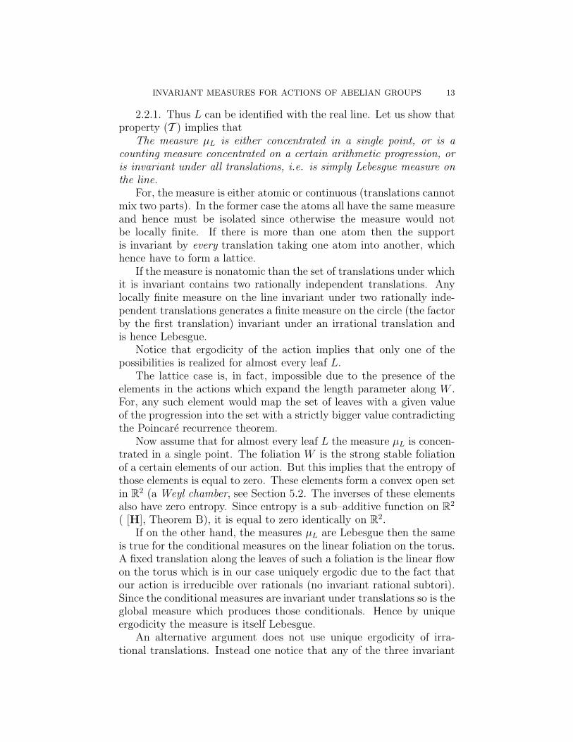
2.2.1. Thus L can be identified with the real line. Let us show thatproperty (T ) implies that
The measure µL is either concentrated in a single point, or is acounting measure concentrated on a certain arithmetic progression, oris invariant under all translations, i.e. is simply Lebesgue measure onthe line.
For, the measure is either atomic or continuous (translations cannotmix two parts). In the former case the atoms all have the same measureand hence must be isolated since otherwise the measure would notbe locally finite. If there is more than one atom then the supportis invariant by every translation taking one atom into another, whichhence have to form a lattice.
If the measure is nonatomic than the set of translations under whichit is invariant contains two rationally independent translations. Anylocally finite measure on the line invariant under two rationally inde-pendent translations generates a finite measure on the circle (the factorby the first translation) invariant under an irrational translation andis hence Lebesgue.
Notice that ergodicity of the action implies that only one of thepossibilities is realized for almost every leaf L.
The lattice case is, in fact, impossible due to the presence of theelements in the actions which expand the length parameter along W .For, any such element would map the set of leaves with a given valueof the progression into the set with a strictly bigger value contradictingthe Poincare recurrence theorem.
Now assume that for almost every leaf L the measure µL is concen-trated in a single point. The foliation W is the strong stable foliationof a certain elements of our action. But this implies that the entropy ofthose elements is equal to zero. These elements form a convex open setin R2 (a Weyl chamber, see Section 5.2. The inverses of these elementsalso have zero entropy. Since entropy is a sub–additive function on R2
( [H], Theorem B), it is equal to zero identically on R2.If on the other hand, the measures µL are Lebesgue then the same
is true for the conditional measures on the linear foliation on the torus.A fixed translation along the leaves of such a foliation is the linear flowon the torus which is in our case uniquely ergodic due to the fact thatour action is irreducible over rationals (no invariant rational subtori).Since the conditional measures are invariant under translations so is theglobal measure which produces those conditionals. Hence by uniqueergodicity the measure is itself Lebesgue.
An alternative argument does not use unique ergodicity of irra-tional translations. Instead one notice that any of the three invariant

14 BORIS KALININ AND ANATOLE KATOK
foliations W1, W2 and W3 can play the role of W in the above argu-ment. Since for any of these there is an element of the action for whichit is the whole stable foliation, if at least one of the three systems ofconditional measures are atomic the entropy of this element and henceof any element of the action vanishes. On the other hand, if all threesystems of conditional measures are Lebesgue, then by Fubini Theoremthe global measure is also Lebesgue.
2.2.2. Now we will explain why property (T ) holds. This is donein two steps.
Step 1. The measures are invariant in the affine sense: the trans-lations are proportional up to a scalar multiple. To that end, let usfix the normalization at µ–almost every point x in such a way that theconditional measure of the interval I(x) of length one on the leaf L(x)centered at x is equal to one. Identifying I(x) with the standard inter-val [0, 1] via the length parameter we obtain a Borel map from our spaceto the set of probability measures on the unit interval provided withthe weak* topology. On a compact subset C of measure arbitrary closeto one this map is continuous (Luzin Theorem). A typical compactpiece of a leaf intersects such a subset by a set of almost full condi-tional measure. Now use our ergodicity assumption (E). Starting froma typical point x on a typical leaf L and moving in the critical directionthe interval I(x) comes arbitrary close to µL almost every point y ∈ L.In particular, if one assumes that both x and y are typical points ofone of the continuity sets C described above, one may assert that thereturns also appear on the set C. But this implies that in the limitthe images of the conditional measures on I(x) weakly converge to theconditional measure on I(y). On the other hand, since we move alongthe critical direction the interval I(x) is simply translated. Hence, thenormalized conditional measure on I(y) coincides with a translation ofthe normalized conditional measure on I(x).
Step 2. The normalization constant which we will denote c(x, y),is in fact equal to one. This again follows from the Poincare recur-rence. For, obviously, this constant is equivariant with respect to theaction: for a ∈ R2, c(α(a)x, α(a)y) = c(x, y). Secondly this is cocycle:c(x, y)c(y, z) = c(x, z). The latter condition implies that along a typ-ical leaf the density is exponential with respect to the natural lengthparameter. Taking an element a for which α(a) contracts the foliationW we see that the exponent must grow contradicting the Poincare re-currence Theorem again, unless it is zero, i.e. the conditional measureis indeed Lebesgue.

INVARIANT MEASURES FOR ACTIONS OF ABELIAN GROUPS 15
2.2.3. Finally, we need to check assumption (E) for any α–invariantergodic measure, namely to show that the ergodic components for theaction in the critical direction consist of the whole leaves of W . Tothat end we will use the structure of stable and unstable foliations fordifferent elements or the action. In fact, for any of the three foliationsthere exists an element a ∈ R2 such that this foliation is the stablefoliation of α(a) and the sum of the other two is the unstable one. Onthe other hand, the classical Hopf argument shows that ergodic decom-position for any element consists of complete leaves of its stable andunstable foliations: the positive (negative) time average of any con-tinuous function is constant along the stable (unstable) leaves. Theremaining ingredient is an important observation that for a normallyhyperbolic (generic) element of the action the measurable hulls of par-titions into leaves of the stable and unstable foliation coincide, becauseeach of them generates the Pinsker σ–algebra (maximal σ–algebra withzero entropy).
Let us denote by ξa the partition into ergodic component of theelement α(a) and by ξ(W ) the measurable hull of the partition intothe leaves of the foliation W . Now let a be a non–zero element inthe critical direction, W ′ be the one–dimensional stable foliation of a,W ′′ be the remaining foliation and b ∈ R2 be a regular (non–critical)element such that W ′ is the stable foliation of the element α(b). Thuswe have the following inequalities:
(2.2.1) ξa ≤ ξ(W ′) = π(α(b)) = ξ(W ⊕W ′′) ≤ ξ(W ).
2.3. ×2, ×3 and automorphisms of a solenoid. A very simi-lar situation appears for commuting expanding maps of the circle. Thebasic example is the action of Z2
+ generated by multiplications by 2and by 3 ( mod 1). The question about invariant measures of thisactions was posed by Furstenberg in 1967 [F]; it was solved for mea-sures with positive entropy by D. Rudolph, [R]. It was an attempt tounderstand Rudolph’s result in a geometric fashion that led the secondauthor to the consideration of the model on the three–torus describedabove. Now in order to prove that the only ergodic positive entropyinvariant measure for the multiplications by 2 and by 3 is Lebesgue wepass to the natural extension for this action. The phase space for thisnatural extension is a solenoid, the dual group to the discrete groupZ(1/2, 1/3). It is locally modeled on the product of R with the groupsof 2–adic and 3–adic numbers. Thus while topologically the solenoid isone–dimensional, there are three Lyapunov exponents, one for the realdirection, and two for the non–Archimedean ones. Since the multipli-cation by 2 is an isometry in the 3–adic norm and vice versa the critical

16 BORIS KALININ AND ANATOLE KATOK
lines in this case are the two axis and the line x log 2+y log 3 = 0 whichdoes not intersect the first quadrant. All the above arguments work inthis case verbatim with the real foliation playing the role of W . Theunique ergodicity of the flow of translations along the real directionfollows form the construction of the solenoid.
This argument of course extends to multiplications by p and q unlessfor some natural numbers k and l, pk = ql.
2.4. Other types of rigidity. . The models discussed in thissection are also very convenient for demonstrating a other types ofrigidity phenomena which appear in actions of higher rank abeliangroups.
The first type is rigidity of vector valued Hoelder and differentiablecocycles. Rigidity in these cases means that every cocycle from a givenclass is cohomologous to a constant coefficient cocycle, i.e. a homomor-phism from the acting group to the vector space with the cohomologygiven by a transfer function from the same class or with moderate loss ofregularity. See [KS1] for 1-cocycles over differentiable actions, [KSch]for 1-cocycles over actions by automorphisms of compact groups and[KK] for higher-order cocycles. A nice survey which also discussesother types of cocycles, such as those with values with compact abeliangroups as well as nonabelian groups is [NT].
Another type of rigidity is local differentiable rigidity: any smoothaction close to a given action in C1 topology is differentiably conjugate(also maybe with a small loss of regularity) to the original action; inthe continuous case up to an automorphism of Rk close to identity (see[KS2]). It is interesting to point that the proof of local differentiablerigidity involves a construction of a certain family of invariant geometricstructures on certain invariant foliations of the perturbed action. Inthe simplest cases this structure is an affine connection. Then thestructural stability implies existence of continuous conjugacy betweenthe original and perturber action (up to a time change in the continuouscase). The principal idea in the proof that the conjugacy must besmooth involves showing that it intertwines a standard structure onthe leaves of an invariant foliation for the algebraic action with thecorresponding structure of the perturbed one. These latter structureplays a role very similar to that of conditional measures in the setupof the present paper.
There are also global rigidity results which assume that an ac-tion has certain topological (e.g. homotopy type) and dynamical (i.e.Anosov) properties and assert conjugacy with a standard algebraic ac-tion [KL, MQ].

INVARIANT MEASURES FOR ACTIONS OF ABELIAN GROUPS 17
The forthcoming notes [K2] discuss all these types of rigidity pri-marily in the simplest setting of actions of Z2 by automorphisms ofT3.
3. Rigidity of invariant measures for actions by toral
automorphisms
3.1. The Main Theorem and its Corollaries. In this sectionwe discuss the main results on the rigidity of invariant measures forhigher rank abelian actions by toral automorphisms. Theorem 3.1 isa modified version of the main result of A. Katok and R. Spatzier forthe case of Zk action by toral automorphisms (Theorem 5.1’ of [KS4],which is in turn a modification of Theorem 5.1 of [KS3]). We givea complete self-contained proof of this theorem which is based on theoriginal proof in [KS3] and [KS4].
The modification reflects the new version of Lemma 5.8’ from [KS4](see Lemma 3.11). The proof of Lemma 5.8’ in [KS4] contains a gapsince the ergodicity of the action may not imply that subspaces Sx areparallel. This in particular forces a slight modification in the formula-tion of the result, namely splitting of the measure into finitely manycomponents. We give a more detailed proof of Lemma 3.2 (Lemma 5.4from [KS3]) and a more elementary proof of Lemma 3.4 (Lemma 5.6from [KS3]). Lemma 3.6 and Lemma 3.8 are similar to Lemma 5.9 andLemma 5.10 in [KS3]. and the proofs employ the idea of the proofs in[KS3]. While the latter lemmas are correct their proofs in [KS3] lacksome essential details. We give new arguments to complete the proofs.
Let α and α′ be actions of Zk by toral automorphisms and let α′
be an algebraic factor of α. Then α′ is called a rank–one factor of αif α′(Zk) has a subgroup of finite index which consists of powers of asingle map.
For an action α of Zk by automorphisms a torus the following twoconditions are equivalent [S].
(R) : The action α contains a subgroup ρ, isomorphic to Z2, whichconsists of ergodic automorphisms.
(R′) : The action α does not possess non–trivial rank one algebraicfactors.
Theorem 3.1. Let α be an Rk-action with k ≥ 2 induced from Zk
action by automorphisms of Tm satisfying condition (R). Assume thatµ is an ergodic invariant measure for α such that there are genericsingular elements a1, . . . , ak and a regular element b ∈ Rk such that

18 BORIS KALININ AND ANATOLE KATOK
C1: : E−b =
∑i(E
0ai∩ E−
b ) (where the sum need not be direct)and
C2: : ξai≤ ξ(E0
ai∩E−
b ).
Then either the invariant measure µTm for the Zk action by auto-morphisms of Tm has zero entropy for all elements of the action or itdecomposes as µTm = 1
N(µ1 + ...+µN), where measures µi, i = 1, ..., N ,
are invariant under α(Γ) for some finite index subgroup Γ ⊂ Zk. Theactions (α(Γ), µi) are algebraically isomorphic by the toral automor-phisms from α(Zk). Each µi, i = 1, ..., N , is an extension of a zeroentropy measure in an algebraic factor for α(Γ) of smaller dimensionwith Haar conditional measures in the fibers.
Condition C2 (which of course depends on C1 while the latter doesnot mean much by itself) is a generalization of the condition (E) formSection 2.1. It will play a similar role in the proof. There are varioussituations where these conditions can be established. It is triviallysatisfied if every one-parameter subgroup of the action α is ergodic, or,equivalently if the original Zk action by toral automorphisms is weaklymixing.
Corollary 3.1. Let α be a Zk-action with k ≥ 2 by automor-phisms of a torus satisfying condition (R). Then any weakly mixinginvariant measure for α is an extension of a zero entropy measure inan algebraic factor with Haar conditional measures in the fibers.
The following corollary of Theorem 3.1 will be used in Section 4.
Theorem 3.2. Let α be an action of Z2 by ergodic toral automor-phisms and let µ be an α–invariant weakly mixing measure such thatfor some m ∈ Z2, α(m) is a K-automorphism. Then µ is a translateof Haar measure on an α–invariant rational subtorus.
Proof. By Theorem 3.1 the measure µ is an extension of a zeroentropy measure for an algebraic factor of smaller dimension with Haarconditional measures in the fiber. Since α contains a K-automorphismit does not have nontrivial zero entropy factors. Hence the factor inquestion is the action on a single point and µ itself is a Haar measureon a rational subtorus. �
In the special case considered in Section 2.2 the ergodicity assump-tion (E) for the critical direction was deduced from ergodicity. The de-duction was based on the interlacing of stable and unstable foliationswhich allowed to produce (2.2.1). Now we will show how a similar

INVARIANT MEASURES FOR ACTIONS OF ABELIAN GROUPS 19
argument allows to verify conditions of Theorem 3.1 in much greatergenerality.
Theorem 3.3. Any ergodic invariant measure µ for a totally non-symplectic Anosov action of Zk by automorphisms of a torus eitherhas zero entropy for all elements of the action or decomposes as µ =1N
(µ1 + ... + µN), where measures µi, i = 1, ..., N , are invariant under
α(Γ) for some finite index subgroup Γ ⊂ Zk. The actions (α(Γ), µi)are algebraically isomorphic by the toral automorphisms from α(Zk).Each µi, i = 1, ..., N , is an extension of a zero entropy measure in analgebraic factor for α(Γ) of smaller dimension with Haar conditionalmeasures in the fibers.
Proof. First for any Anosov TNS action of Zk, k ≥ 2, since fork = 1 any positive exponent is negatively proportional to any negativeexponent. Thus we need to check conditions C1, C2. For that itis obviously sufficient to show that for any generic singular elementa ∈ Rk, ξa ≤ ξ(E0
a).For such an element a a single Lyapunov exponent vanishes and the
corresponding Lyapunov distribution coincides with E0a. Take a regular
element b nearby for which the corresponding Lyapunov exponent ispositive and all other exponents have the same signs as for a. ThusE+
b = E+a ⊕ E0
a and E−b = E−
a . Birkhoff averages with respect to α(a)of any continuous function are constant on the leaves of ξa. Since suchaverages generate the algebra of α(a) invariant functions we concludethat ξa ≤ ξ(E−
a ). On the other hand both and both ξ(E−b ) and ξ(E+
b )coincide with the Pinsker algebra π(α(b)). Thus we conclude
ξa ≤ ξ(E−a ) = ξ(E−
b ) = π(α(b)) = ξ(E+b ) = ξ(E+
a ⊕ E0a) ≤ ξ(E0
a).
�
Corollary 3.2. Any ergodic invariant measure for an irreducibletotally nonsymplectic Anosov action of Zk by automorphisms of a toruseither has zero entropy for all elements of the action or is Lebesguemeasure on the torus.
3.2. Scheme of the Proof of Theorem 3.1. Step 1. Let usconsider one of the generic singular elements ai from the statement ofTheorem 3.1 and a Lyapunov exponent λ such that λ(ai) = 0. Wedenote by F the invariant foliation W I
ai∩W−
b ∩W λ where W λ is theLyapunov foliation corresponding to λ.
In Section 3.3 we use Lemmas 3.2, 3.3, 3.4 to establish the followingdichotomy.

20 BORIS KALININ AND ANATOLE KATOK
Lemma 3.1. For any foliation F described above either
(1) The conditional measure µFx is atomic for µ-a.e. x, or
(2) The conditional measure µFx is a Haar measure on an affine
subspace Sx of positive dimension for µ-a.e. x.
Step 2. If for all foliations F described in Step 1 the first alterna-tive of Lemma 3.1 takes place then we prove in Section 3.4 that theconditional measures on the foliation W−
b are atomic. By Proposition1.1 this implies that the entropy of α(b) is equal to 0. Since the stablefoliation is the same for all elements in the same Weyl chamber we seethat the entropy is 0 for all elements in the same Weyl chamber as b.Since the entropies of α(b) and α(−b) are the same we conclude theentropy is 0 for all elements in the Weyl chamber of b. Then it followsfrom sublinearity of entropy [H] that all elements of the action have 0entropy.
This completes the proof of Theorem 3.1 in the case when the firstalternative of Lemma 3.1 takes place for all foliations F described inStep 1.
Step 3. Suppose that for some foliation F described in Step 1 thesecond alternative of Lemma 3.1 takes place, i.e. the conditional mea-sure µF
x is a Haar measure on an affine subspace Sx for µ-a.e. x. Wenote that by ergodicity of the action the subspaces Sx have the samedimension for µ-a.e. x. We may assume that this dimension is positive.Then Lemma 3.11 shows that the measure on the torus decomposes asµTm = 1
N(µ1 + ... + µN), where measures µi, i = 1, ..., N , are invari-
ant under α(Γ) for some finite index subgroup Γ ⊂ Zk. The actions(α(Γ), µi) are algebraically isomorphic and each µi, i = 1, ..., N , is anextension of a zero entropy measure in an algebraic factor of smallerdimension for α(Γ) with Haar conditional measures in the fibers. Werestrict the action α to the finite index subgroup Γ and consider invari-ant measure µ1. If the factor–measure has zero entropy for all elementsof this action we are done. Otherwise we may assume that in the fac-tor some element still has positive entropy and repeat the argument.Note that condition (R) is inherited by any algebraic factor as well asconditions C1, C2. We will arrive at a factor of the factor and so on.Since at every step the dimension of the factor drops this process hasto stop, thus producing a factor with zero entropy. It is also clear byinduction that the conditionals are in fact Haar measures on the fibers.
Notice that in the case of Z2 action on T3 considered in Section 2.2Steps 2 and 3 are not needed.

INVARIANT MEASURES FOR ACTIONS OF ABELIAN GROUPS 21
3.3. Proof of the Lemma 3.1. In this section we prove the fol-lowing three lemmas from [KS3] which establish the dichotomy ofLemma 3.1 from Section 3.2. Lemma 3.2 generalizes the argumentfrom the Step 1 in Section 2.2.2, and Lemma 3.4 the argument fromStep 2 in the same section.
The general setup for these lemmas is as follows. Suppose thata ∈ Rk is a generic singular element and F ⊂W I
a is some α(a)-invariantsubfoliation of W I
a with leaves of dimension d. Denote by BF1 (x) the
closed unit ball in F (x) about x with respect to the flat metric. Denoteby µF
x the system of conditional measures on F normalized by therequirement µx(B
F1 (x)) = 1 for all x in the support of µ and by Gx
the subgroup of isometries of F (x) which preserve µFx up to a scalar
multiple.To simplify the notation from now on we will write a instead of
α(a) when this does not cause any confusion.Recall that we denote by ξa the partition into ergodic components
of element a and by ξ(F ) the measurable hull of F .
Lemma 3.2. ([KS3], Lemma 5.4) Suppose that ξa ≤ ξ(F ). Thenfor µ-a.e. x, Gx is closed and the support of µF
x is the orbit of x underthe group Gx . Furthermore, φ∗µ
Fx = µF
φx for any φ ∈ Gx.
Proof. To prove the last statement of the lemma we note that thenormalizations of the conditional measures φ∗µ
Fx and µF
y coincide since
φ∗µFx (BF
1 (y) = µFx (BF
1 (x)) = 1 due to the fact that φ is an isometry.Since Gx maps the support of µF
x to itself we only need to showthat Gx is closed and acts transitively on the support of µF
x .We first show that Gx is closed. Let {φn} ⊂ Gx be a sequence of
isometries converging to an isometry φ. We need to show that φ ∈Gx. Let yn = φn(x) and y = φ(x). We can choose a radius r suchthat the boundaries of balls BF
r (x) and BFr (y) carry no conditional
measure. Let us denote by µF,rz the conditional measure normalized
by µF,rz (BF
r (z)) = 1. Since the balls BFr (yn) converge to BF
r (y) weconclude that µF,r
ynconverge to µF,r
y in weak* topology. Since φn ∈ Gx
we see that (φn)∗µF,rx = µF,r
ynsince their normalizations coincide. Since
(φ)∗µF,rx is the weak* limit of (φn)∗µ
F,rx it follows that (φ)∗µ
F,rx = µF,r
y .
Since µF,ry is a scalar multiple of µF,r
x , we conclude that φ belongs toGx.
It remains to show that for µ-a.e. x and µFx -a.e. y ∈ F (x) there
exists an isometry φ of F (x) such that y = φ(x) and µFy = φ∗µ
Fx . Since
Gx is closed and any set of full measure is dense in the support of µFx ,
it would follow that Gx is, in fact, transitive on the support of µFx .
22 BORIS KALININ AND ANATOLE KATOK
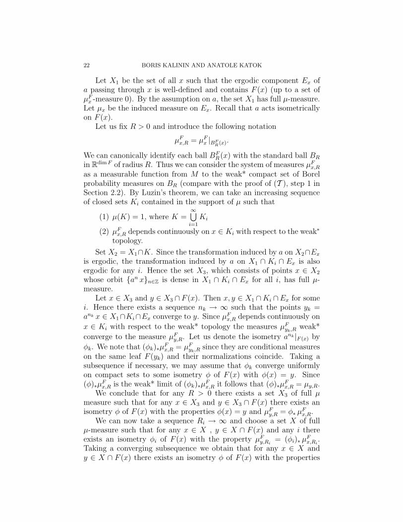
Let X1 be the set of all x such that the ergodic component Ex ofa passing through x is well-defined and contains F (x) (up to a set ofµF
x -measure 0). By the assumption on a, the set X1 has full µ-measure.Let µx be the induced measure on Ex. Recall that a acts isometricallyon F (x).
Let us fix R > 0 and introduce the following notation
µFx,R = µF
x |BFR
(x).
We can canonically identify each ball BFR(x) with the standard ball BR
in Rdim F of radius R. Thus we can consider the system of measures µFx,R
as a measurable function from M to the weak* compact set of Borelprobability measures on BR (compare with the proof of (T ), step 1 inSection 2.2). By Luzin’s theorem, we can take an increasing sequenceof closed sets Ki contained in the support of µ such that
(1) µ(K) = 1, where K =∞⋃i=1
Ki
(2) µFx,R depends continuously on x ∈ Ki with respect to the weak∗
topology.
Set X2 = X1∩K. Since the transformation induced by a on X2∩Ex
is ergodic, the transformation induced by a on X1 ∩ Ki ∩ Ex is alsoergodic for any i. Hence the set X3, which consists of points x ∈ X2
whose orbit {an x}n∈Z is dense in X1 ∩ Ki ∩ Ex for all i, has full µ-measure.
Let x ∈ X3 and y ∈ X3 ∩F (x). Then x, y ∈ X1 ∩Ki ∩Ex for somei. Hence there exists a sequence nk → ∞ such that the points yk =ank x ∈ X1∩Ki∩Ex converge to y. Since µF
x,R depends continuously on
x ∈ Ki with respect to the weak* topology the measures µFyk,R weak*
converge to the measure µFy,R. Let us denote the isometry ank |F (x) by
φk. We note that (φk)∗µFx,R = µF
yk,R since they are conditional measureson the same leaf F (yk) and their normalizations coincide. Taking asubsequence if necessary, we may assume that φk converge uniformlyon compact sets to some isometry φ of F (x) with φ(x) = y. Since(φ)∗µ
Fx,R is the weak* limit of (φk)∗µ
Fx,R it follows that (φ)∗µ
Fx,R = µy,R.
We conclude that for any R > 0 there exists a set X3 of full µmeasure such that for any x ∈ X3 and y ∈ X3 ∩ F (x) there exists anisometry φ of F (x) with the properties φ(x) = y and µF
y,R = φ∗ µFx,R.
We can now take a sequence Ri → ∞ and choose a set X of fullµ-measure such that for any x ∈ X , y ∈ X ∩ F (x) and any i thereexists an isometry φi of F (x) with the property µF
y,Ri= (φi)∗ µ
Fx,Ri
.Taking a converging subsequence we obtain that for any x ∈ X andy ∈ X ∩ F (x) there exists an isometry φ of F (x) with the properties

INVARIANT MEASURES FOR ACTIONS OF ABELIAN GROUPS 23
φ(x) = y and µFy = φ∗ µ
Fx . This completes the proof of the lemma since
we may assume that the set X is chosen so that for x ∈ X the setX ∩ F (x) has full µF
x -measure. �
Lemma 3.3. ([KS3], Lemma 5.5) In addition to the assumptionsin Lemma 3.2, let F be contained in the intersection of W I
a with aLyapunov subspace for a non-zero Lyapunov exponent λ. Then forµ-a.e. x, the support Sx of µF
x is an affine subspace of F (x) whosedimension is constant for almost every x..
Proof. By Lemma 3.2, Sx is the orbit of a closed group of isome-tries. Therefore Sx is a submanifold, possibly disconnected. Note thatthe maximal principal curvature of Sx is constant along Sx. Let κ(x)denote this constant.
Let b be any element such that λ(b) < 0. Note that b maps Sx
to Sb x. Iterates of b exponentially contract the fibers of F . In partic-ular, since the exponential contractions in all directions inside F arethe same, any curve with positive principal curvature will be mappedto curves with exponentially increasing principal curvatures. Henceκ(bnx) goes to infinity for µ-a.e. x unless κ(x) = 0. This is impossibleby Poincare recurrence. Thus κ(x) ≡ 0, and hence the support of µF
x
is a union of non-intersecting affine subspaces.Let us now show that the support is connected. Suppose to the
contrary that the support is a union ∪Ai of at least two affine subspacesAi. Let dx denote the minimum of the distances from x to any Ai whichdoes not contain x. Since the support is a closed subset, dx > 0 for allx. Note that dbn x → 0 as n → ∞. This is again a contradiction toPoincare recurrence. The dimension of Sx is α-invariant and hence isconstant due to the ergodicity of the action α. �
Lemma 3.4. ([KS3], Lemma 5.6) Under the assumptions of Lemma 3.3,µF
x is Haar measure on Sx.
Proof. By Lemma 3.2 the group Gx of isometries of F (x) whichmap µF
x to its scalar multiple acts transitively on the support Sx of theconditional measure of µF
x . By Lemma 3.3, Sx is an affine space. Forany x and y ∈ Sx ⊂ F (x) let us define the scaling coefficient cx(y) bythe equality φµF = cx(y)µ
F , where µF is the conditional measure onF (x) = F (y) and φ ∈ Gx is an isometry such that φ(x) = y. In otherwords cx(y) can be calculated as
cx(y) =φ∗µ
F (A)
µF (A)=µF (φ−1A)
µF (A)=
µF (A)
µF (φA)
for any set A of positive conditional measure. We note that since theconditional measures are defined up to a scalar multiple it is clear that

24 BORIS KALININ AND ANATOLE KATOK
the definition does not depend on a particular choice of µF . Since theimage of the unit ball φ(BF
1 (x)) is the same for all isometries φ ∈ Gx
such that φ(x) = y we conclude that the definition does not depend ona particular choice of φ either.
Since we can take the test set A such that the conditional measureof the relative (to F (x)) boundary of φA is equal to zero, we concludethat that for a fixed x the coefficient cx(y) depends continuously on y.
We see that either for µ − a.e. x cx(y) = 1 for all y ∈ Sx, henceµF
x is Haar on Sx, or there exists a set X of positive measure such thatcx(y) is not identically equal to 1 for x ∈ X. In the latter case for someǫ > 0 we can define a finite positive measurable function
fǫ(x) = inf{r : ∃ y ∈ Sx s.t. d(x, y) < r and |cx(y) − 1| > ǫ}
on some subset Y ⊂ X of positive µ-measure. By measurability thereexists N and a set Z of positive measure on which fǫ takes values inthe interval (1/N,N). We will show that
(3.3.1) fǫ(bnx) → 0 as n→ ∞
uniformly on Z for an element b which contracts foliation F . This willprove the lemma since it contradicts to the recurrence of Z under b.
We will prove now that
(3.3.2) cx(y) = cbx(by)
for µ-a.e. x and y ∈ Sx. Since the iterates of b exponentially con-tract the leaves of F this invariance property implies that fǫ(b
nx) ≤Cλnfǫ(x), for some C,λ > 0, hence (3.3.2) implies (3.3.1)
To prove (3.3.2) we use Lemma 3.2. For any y ∈ Sx there existsan isometry φ of F (x) with the properties φ(x) = y and µF
y = (φ)∗ µFx .
Since such φ can be obtained as a limit of a sequence of some powersof a restricted to F (x) we may assume that it commutes with b in thefollowing sense. The map ψ = b◦φ ◦ b−1 is an isometry of F (bx). Thuswe have b ◦ φ = ψ ◦ b. We note that since b preserves the family ofconditional measures (up to a scalar multiple) ψ preserves the condi-tional measures on F (bx) up to a scalar multiple. Hence for any setA ⊂ F (x) of positive conditional measure we have
cx(y) =µF (A)
µF (φA)=
(b∗µF )(bA)
(b∗µF )(b ◦ φA)=
=(b∗µ
F )(bA)
(b∗µF )(ψ ◦ bA)=
(b∗µF )(bA)
(b∗µF )(ψ(bA))= cbx(by).
�

INVARIANT MEASURES FOR ACTIONS OF ABELIAN GROUPS 25
3.4. The Case of Atomic Conditional Measures. In this sec-tion we consider the case when for all foliations F , described in Step1 of the scheme of the proof, the first alternative of Lemma 3.1 takesplace, i.e. the conditional measures are atomic. We use Lemmas 3.5,3.6, and 3.8 to show that in this case the conditional measures on thefoliation W−
b are atomic. This by Proposition 1.1 implies that the en-tropy of α(b) is equal to 0 and allows us to proceed as in Step 2 of thescheme of the proof.
Remark 3.1. This part of the argument is not needed in the caseconsidered in Section 2.2 since the foliation F in that case coincideswith the complete stable foliation of some regular element b and hencezero entropy follows right away.
As in Step 1 of the scheme of the proof of Theorem 3.1 we con-sider one of the generic singular elements ai from the statement ofTheorem 3.1 and a Lyapunov exponent λ such that λ(ai) = 0. Let usdenote by F the invariant foliation W I
ai∩W−
b ∩W λ where W λ is theLyapunov foliation corresponding to λ. We know that the conditionalmeasure µF
x is atomic for µ-a.e. x.First we use Lemma 3.5 to conclude that the conditional mea-
sures on the foliation W Iai∩W−
b are atomic for each ai. We note thatLemma 3.2 implies that the conditional measures on the whole foliationW I
ai∩W−
b are supported on smooth submanifold of the leaves.
Once we know that the conditional measures on foliations W Iai∩W−
b
for all i are atomic Lemma 3.6 shows that the conditional measureson all foliations W 0
ai
⋂W−
b are also atomic. Then to show that theconditional measures on the whole W−
b are atomic we use the inductiveprocess as in the end of the outline of the proof of Theorem 5.1 in [KS3].
We restrict the action to a 2-plane which contains b and intersectsall the Lyapunov hyperplanes in generic lines. Then we can replaceeach ai by an element ci in the intersection of the 2-plane with theunique Lyapunov hyperplane that contains ai. Since the elements ai
and ci have the same center foliation for each i we see that
E−b =
∑
i
(E0ai∩ E−
b ) =∑
i
(E0ci∩ E−
b )
and the conditional measures on all W 0ci∩W−
b are atomic. We can nowreorder the elements ci in such a way that the Lyapunov exponent thatcorrespond to E0
cj∩ E−
b is negative on ci for each j < i. Starting with
W 0c1∩W
−b we apply Lemma 3.8 inductively to prove that the conditional
measures are atomic on (W 0c1⊕W 0
c2)∩W−
b , on (W 0c1⊕W 0
c2⊕W 0
c3)∩W−
b ,and so on until we exhaust the whole W−
b .
26 BORIS KALININ AND ANATOLE KATOK
To complete the proof that the conditional measures on the foliationW−
b are atomic we need to prove Lemmas 3.5, 3.6, and 3.8 below.
The proof of Lemma 3.5 follows the proof of Lemma 5.8 in [KS3].Lemma 3.6 is identical to Lemma 5.9 in [KS3] and Lemma 3.8 is aslight modification of Lemma 5.10 from [KS3].
Notice that any α-invariant subfoliation of W Ia splits into its inter-
sections with Lyapunov foliations.
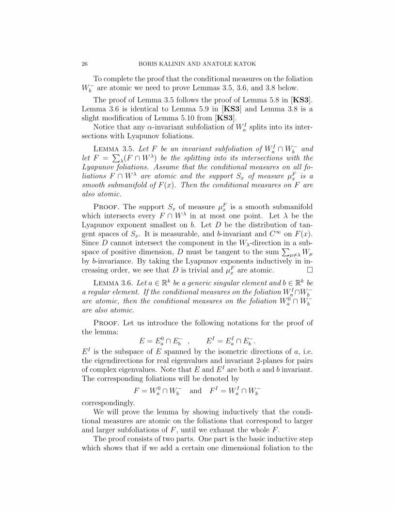
Lemma 3.5. Let F be an invariant subfoliation of W Ia ∩W−
b andlet F =
∑λ(F ∩ W λ) be the splitting into its intersections with the
Lyapunov foliations. Assume that the conditional measures on all fo-liations F ∩ W λ are atomic and the support Sx of measure µF
x is asmooth submanifold of F (x). Then the conditional measures on F arealso atomic.
Proof. The support Sx of measure µFx is a smooth submanifold
which intersects every F ∩ W λ in at most one point. Let λ be theLyapunov exponent smallest on b. Let D be the distribution of tan-gent spaces of Sx. It is measurable, and b-invariant and C∞ on F (x).Since D cannot intersect the component in the Wλ-direction in a sub-space of positive dimension, D must be tangent to the sum
∑µ6=λ Wµ
by b-invariance. By taking the Lyapunov exponents inductively in in-creasing order, we see that D is trivial and µF
x are atomic. �
Lemma 3.6. Let a ∈ Rk be a generic singular element and b ∈ Rk bea regular element. If the conditional measures on the foliation W I
a ∩W−b
are atomic, then the conditional measures on the foliation W 0a ∩W−
b
are also atomic.
Proof. Let us introduce the following notations for the proof ofthe lemma:
E = E0a ∩E−
b , EI = EIa ∩E−
b .
EI is the subspace of E spanned by the isometric directions of a, i.e.the eigendirections for real eigenvalues and invariant 2-planes for pairsof complex eigenvalues. Note that E and EI are both a and b invariant.The corresponding foliations will be denoted by
F = W 0a ∩W−
b and F I = W Ia ∩W−
b
correspondingly.We will prove the lemma by showing inductively that the condi-
tional measures are atomic on the foliations that correspond to largerand larger subfoliations of F , until we exhaust the whole F .
The proof consists of two parts. One part is the basic inductive stepwhich shows that if we add a certain one dimensional foliation to the

INVARIANT MEASURES FOR ACTIONS OF ABELIAN GROUPS 27
previously constructed foliation than the conditional measures will beagain atomic. This part is established in Lemma 3.7. The other partis the inductive process itself which we explain below. In this part wechoose the one dimensional directions and the proper ordering of themto ensure our ability to make the inductive step. This choice is basedon the relation between the algebraic properties of elements a and b aslinear transformations of E.
The a and b invariant subspace E splits as the direct sum of itsintersections with the root subspaces (the generalized eigenspaces) ofa:
E =⊕
λ∈Sp(a)
Ker(a− λ)m.
Each term of this direct sum is b invariant since b commutes witha. Hence it can be split into the direct sum of root subspaces for therestriction of b. Thus we obtain the splitting E =
⊕Ui which is invari-
ant under both elements a and b. Let us denote by λi (correspondinglyνi) the eigenvalue of a (correspondingly b) on the subspace Ui. We havethat |λi| = 1 and |νi| < 1 for all i. Each Ui is filtered as
Ui ∩ EI = V 0
i ⊂ ... ⊂ V di
i = Ui , where V ki = Ker(a− λi)
k+1 ∩ Ui
and (di+1) is the maximal dimension of Jordan blocks of a on Ui. Notethat since b commutes with a it leaves each subspace V k
i invariant. Sowe see that each V k
i is both a and b invariant. We assign the ”weight”
|νi|1j to each subspace V j
i , we assign 0 weight to subspace V 0i . Let us
enumerate the weights in the increasing order: 0 = w0 < w1 < ... < wj0.We denote by Ej the direct sum of all V k
i whose weights equal to wj.Now E filtrates as
EI = E0 ⊂ ... ⊂ Ej0 = E.
Even though the subspaces V ki that correspond to the complex
eigenvalues are defined only over C all subspaces Ej are defined over R.This follows from the structure of the Jordan normal form for a overreals. We note again that each Ej is a and b invariant.
We will show inductively that the conditional measures on the fo-liations corresponding to Ej are atomic.
Let us fix j and assume inductively that the conditional measureson the foliation corresponding to Ej−1 are atomic. We will prove thatthe conditional measures on the foliation corresponding to Ej are alsoatomic by showing that the conditional measures are atomic on thefoliations corresponding to larger and larger subspaces of Ej . Thedimension of the subspace will be increased by one at each step untilwe exhaust the whole Ej.

28 BORIS KALININ AND ANATOLE KATOK
When we would like to add one direction in some Ui for which λi
or νi is not real, instead of elements a and b we will use their suitablepowers asi and bti s.t. λsi
i = 1 and 0 < νtii < 1. By taking the
square of the element, if necessary, we may assume that there exist reallogarithms and hence real powers of a and b. The ergodicity of theseelements is not needed since we only will be using the fact that theypreserve the measure. Note that the splitting E =
⊕Ui and filtrations
Ui ∩EI = V 0i ⊂ ... ⊂ V di
i = Ui are the same for all such powers. Hencethe order of weights and filtration EI = E0 ⊂ ... ⊂ Ej0 = E are alsothe same.
Ej splits into its intersections with Ui as Ej =⊕
V ki
i . Then the
intersections of Ej−1 with Ui are either V ki
i or V ki−1i . We will consider
only the intersections of Ej with Ui of the second type since we do notneed to add any directions along the other Ui’s. The operator (bti −νti
i )
is nilpotent on V ki
i /V ki−1i since it is nilpotent on Ui. Let d1
i , ..., di,Pibe
the dimensions of the cyclic subspaces of (bti − νtii ) on V ki
i /V ki−1i and
ei,1, ..., ei,Pi∈ V ki
i be some representatives of their generators. Thenthe vectors
eli,p := (bti − νti
i )dpi −(l+1)ei,p for p = 1, ..., Pi and l = 0, ..., dp
i − 1
form a basis of V ki
i relative to V ki−1i . Finally we have
Ej = Ej−1 ⊕⊕
i
Pi⊕
p=1
dpi −1⊕
l=0
< eli,p >
We will add the directions < eli,p > to Ej−1 one by one in the order
of increasing of the value of lki
. The rest of the proof describes theprocedure of adding.
Let D =< el0i0,p0
> be the new direction to be added at this step.
We introduce the following notations for this step: k0 := ki0 , el := eli0,p0
for l = 0, ..., l0, A := asi0 and B := bti0 . The eigenvalues of A and Bon Ui0 are correspondingly 1 and ν, where 0 < ν < 1. The vectorsek
l := (A − 1)k0−kel for l = 0, ..., l0 and k = 0, ..., k0 form a Jordannormal basis for A on some subspace V ⊂ Ui which will be of particularinterest for this step. Note that the subspaces Ui0 and V are invariantfor A and B as subspaces over R.
Let us denote by D1 the A and B invariant subspace which is thesum of Ej−1 and previously added directions. We denote the corre-sponding foliation by F1. We assume inductively that the conditional

INVARIANT MEASURES FOR ACTIONS OF ABELIAN GROUPS 29
measures on the foliation F1 are atomic. It is easy to see that the sub-space D2 = D1 ⊕D is also defined over R and both A and B invariant.Let us denote the corresponding foliation by F2.
To complete the proof Lemma 3.6 it remains to prove the followinglemma which shows that the conditional measures on the foliation F2
are atomic.
Lemma 3.7. If the conditional measures on the foliation F1 areatomic then the conditional measures on the foliation F2 are also atomic.
Proof. Let us consider a measurable partition, subordinate to F2,which consists ”mainly” of small ”rectangles” of the same size withsides parallel to the basis directions and has the following property.The measure of the set Intγ is at least 0.99 for some γ > 0, where Intγconsists of points inside rectangles on the distance at least γ from therelative (to the leaf of F2) boundary of the rectangle that contains thepoint.
By induction hypothesis there exists a set of full measure whichintersects any fiber of F1 in at most one point. Approximating thisset from inside we can find a compact set K with the same property.We would like to consider only ”good” part of the measure µ, so weintroduce a new measure µX by µX(.) = µ(. ∩ X), where X = K ∩Intγ with µ(X) ≥ 0.98. Let us consider the system of the conditionalmeasures of µX w.r.t. the measurable partition into the rectangles(the remaining elements have µX measure 0). These measures will bereferred to as the conditional measures of rectangles. We will regardeach rectangle as a direct product of its vertical (F1) and horizontal(D) directions. We observe the following dichotomy:
(1) Either for every rectangle, in a set of positive measure, atleast 1/3 of its conditional measure is concentrated on a singlevertical leaf, hence at one point,
(2) Or there exists a lower bound d > 0 for the width of a verticalstrip of a rectangle that can carry at least 1/3 of its conditionalmeasure, for any rectangle in a set Y consisting of whole rect-angles with µx(Y ) > 0.97
In the first case the existence of atoms for the conditional measuresof rectangles implies the existence of atoms for the conditional measureson foliation F2. Since this foliation is contracted by b the existence ofatoms forces the conditional measures on F2 be atomic. This can beseen as in the proof of Proposition 4.1 in [KS3]. If x is an atom ofthe conditional measure then there exists a small neighborhood U ofx in the leaf F2(x) such that µF2
x (U − {x}) < εµF2x ({x}). Pushing µF2
x

30 BORIS KALININ AND ANATOLE KATOK
backward and using Poincare recurrence, we see that for a typical x,µF2
x is concentrated at x.In the latter case each rectangle in Y can be split into three vertical
strips of width at least d so that both the left and the right ones havethe conditional measure at least 1/3. We again may assume that theconditional measures do not have atoms since otherwise we could argueas in the first case.
The intersection of the compact set K with any rectangle is a graphof a continuous (not necessarily everywhere defined) function from thevertical direction to horizontal. Moreover the family of these functionsis equicontinuous. Let us take some ǫ and find δ given by the equicon-tinuity. Combining contraction provided by B and shear provided byA we will find such an element AmBn that the image of any rectanglefrom Y has the following properties:
(1) The image is δ-narrow in the horizontal direction(2) The distance along the vertical direction between the images
of the right and the left strips is at least ǫ(3) The image is sufficiently small (its diameter less than γ) so
that it can not intersect γ-interiors of two different rectanglessimultaneously.
Under these conditions the images of the right and the left stripscan not intersect Z = X ∩ Y simultaneously. But this implies thatµX(AmBn(Z)∩Z) ≤ 2
3µX(Z) which is impossible since µ(Z) = µX(Z) =
µX(Y ) ≥ 0.97. To prove that the conditional measures on F2 are atomicit remains to show that such an element AmBn exists.
To satisfy the second condition we obtain the required shear alongthe direction of the eigenvector e00. On subspace V element B providesuniform contraction by factor ν and possibly some shear. Since noshear accumulates in V along D =< el0 > direction the size along Ddirection of the image under Bn of any rectangle is νn s, where s isthe size of the original rectangle. Since with respect to B vector el0
has height l0 over e0 the distance between the images under Bn of theright and left strips along e0 direction is at least c0n
l0νnd for somesmall c0 > 0 and sufficiently large n. After this we apply Am, wherem will be exponential in n. We see that the size along D direction isstill νn s. Since vector e0 has height k0 (with respect to A) the leadingterm of the distance between the images of the right and left stripsunder AmBn along the direction of the eigenvector e00 is c1m
k0nl0νnd.Indeed, the other terms with the same power of m have smaller powerof n while terms with smaller power of m are negligible since m willbe exponential in n. We see that the other terms are bounded by

INVARIANT MEASURES FOR ACTIONS OF ABELIAN GROUPS 31
C2mk0nl0−1νns, where C2 is large (depending only on the structure of
the subspace V for A and B), so the distance between the images ofthe right and left strips along e00 direction is at least c3m
k0nl0νnd forsufficiently large m and n and some small c3 (depending only on k0
and l0). Similarly, the size of the image along all V directions can beestimated from above by C4m
k0nl0νns.We would like to show that we can control the size of the image
along other directions in E1 as effectively as along the V directions.For each i the intersection D1∩Ui splits further into A and B invariantreal subspaces that can be constructed similarly to V starting fromsome el
i,p ∈ D1 such that el+1i,p /∈ D1.
Let us consider any one of these A and B invariant real subspacesand denote it by V ′ ⊂ D1 ∩ Ui. As above, we can estimate the sizeof the image along V ′ by C5m
kinl∗ν
n∗ s, where ν∗ is the corresponding
eigenvalue of b.We will now specify the choice of the element AmBn. First we note
that the size of the image of any rectangle along D direction is νn sindependently on m. Hence the condition (1) will be automaticallysatisfied once n is chosen sufficiently large.
We observe that the ratio of the desired shear and the size alongV directions is bounded. To make the shear and the size along Vdirections bounded for large m and n we take m and n so that m ∼
(nl0νn)− 1
k0 . In this case we will obtain the following estimate of thesize of image along the subspace V ′:
C6(ν1ki∗ /ν
1k0 )
kin
nk0( l
ki−
l0k0
)s.
We observe that this estimate is also bounded since ν1ki∗ = ν
1k0 and
lki< l0
k0due to the the ordering of weights and the order of adding
directions inside Ej . Note that if V ′ is constructed starting from some
basis vector in Ej−1 then ν1ki∗ < ν
1k0 due to the ordering of weights and
the estimate will be in fact exponentially small.We conclude that by taking m and n large and so that m ∼
(nl0νn)− 1
k0 we can satisfy the condition (1) for any δ while produc-ing the shear bounded below and the size of the images of rectanglesbounded above. Then given the desired bound γ on the size of theimage we can apply a bounded number of iterates of b to adjust theabove estimate for the size to be γ. After that we choose ǫ smaller thanthe adjusted lower bound for the shear. For this ǫ there exists someδ by the equicontinuity. The above considerations show that we can

32 BORIS KALININ AND ANATOLE KATOK
now take n sufficiently large and m ∼ (nl0νn)− 1
k0 to satisfy all threeconditions. �
This finishes the proof of Lemma 3.6. �
Lemma 3.8. Let W be an invariant subfoliation of W 0a and F be
an invariant subfoliation of W−a for some element a. Suppose that
F ⊕W ⊂ W−b for some element b and that the conditional measures
of µ on both foliations F and W are atomic. Then the conditionalmeasures on the foliation F ⊕W are also atomic.
Proof. We will reduce the lemma to its special case, Lemma 3.9.the reduction goes as follows. Denote W I = W ∩W I
a . Then Lemma 3.9shows that the conditional measures on the foliation F ⊕W I are alsoatomic.
After that we add root directions of W as in Lemma 3.6 and provethat the conditional measures on F ⊕ W are also atomic. The onlydifference is that in the basic step, Lemma 3.7, we need to control thesize of the images of rectangles not only alongW I and previously addedroot directions but also along F directions. But such control is trivialsince by the conditions of the lemma F is contracted by both b and a.
Lemma 3.9. Let W be an invariant subfoliation of W Ia and F be
an invariant subfoliation of W−a for some element a. Suppose that
F ⊕W ⊂ W−b for some element b and that the conditional measures
of µ on both foliations F and W are atomic. Then the conditionalmeasures on the foliation F ⊕W are also atomic.
Proof. Similar to Lemma 3.6 we prove this lemma inductively byadding one dimensional subfoliations of W to the foliation F one untilwe exhaust the whole F ⊕W . Lemma 3.10 shows that on each step ofthis process we obtain a foliation with atomic conditional measures.
Let us consider the Jordan normal form of b on the subspace thatcorresponds to foliation W . This subspace splits over C into the sum⊕
Ui of root subspaces of b. Each Ui is an eigenspace of a correspondingto some eigenvalue λi with |λi| = 1. We denote by νi the correspondingeigenvalue of b.
In order to add a one dimensional direction inside some specificUi for which λi or νi is complex we replace elements a and b by theirproper powers asi and bti to make the corresponding eigenvalues real:λsi
i = 1 and 0 < νtii < 1. This allows us to consider Ui as a subspace
over R.Unlike Lemma 3.6, for this proof we do not need to follow any
particular order of adding. We need only to make sure that when we

INVARIANT MEASURES FOR ACTIONS OF ABELIAN GROUPS 33
add a new direction in some Ui we again obtain a subspace which isboth a and b invariant and defined over R. The desired partial orderingof directions can be obtained by fixing some Jordan normal basis forthe real operator bti on Ui.
The next lemma proves the inductive step and completes the proofof Lemma 3.9.
Lemma 3.10. Let F1 and F2 be invariant subfoliation of W Ia and F
be an invariant subfoliation of W−a for some element a. Suppose that
F2 is one-dimensional, (F ⊕ F1 ⊕ F2) ⊂ W−b for some element b, and
that the conditional measures of µ on both foliations F1⊕F2 and F⊕F1
are atomic. Then the conditional measures on the foliation F ⊕F1⊕F2
are also atomic.
Proof. Since the conditional measures on the foliations F1 ⊕ F2
and F ⊕ F1 are atomic we can find a set of full measure and its com-pact subset K of measure at least 0.99 which intersect any leaf of thefoliations F1 ⊕ F2 and F ⊕ F1 in at most one point.
Consider a measurable partition, subordinate to F⊕F1⊕F2 , whichconsists ”mainly” of small ”rectangles” of the same size with sidesparallel to the foliations F , F1 and F2 and has the following property:the measure of the set Intγ is at least 0.99 for some γ > 0, where Intγconsists of points inside rectangles on the distance at least γ from therelative (to the leaf of F ⊕ F1 ⊕ F2) boundary of the rectangle thatcontains the point.
We would like to consider only ”good” part of the measure µ, sowe introduce a new measure µX by µX(.) = µ(. ∩X), where X = K ∩Intγ with µ(X) ≥ 0.98. Let us consider the system of the conditionalmeasures of µX w.r.t. the measurable partition into the rectangles(the remaining elements have µX measure 0). These measures will bereferred to as the conditional measures of rectangles. We regard eachrectangle as a direct product of its F , F1 and F2 directions. We observethe following dichotomy:
(1) Either for every rectangle, in a set of positive measure, atleast 1/3 of its conditional measure is concentrated on a singleF ⊕ F1 leaf, hence at one point,
(2) Or there exists a set Y with µX(Y ) > 0.97 which consistsof whole rectangles and a number d > 0 such that for anyrectangle in Y any subrectangle that carries at least 1/3 of theconditional measure has width at least d along F2-direction.
In the first case the existence of atoms for the conditional measuresof rectangles implies the existence of atoms for the conditional measures

34 BORIS KALININ AND ANATOLE KATOK
on foliation F ⊕ F1 ⊕ F2. As in the proof of Lemma 3.7 we see thatsince this foliation is contracted by b the existence of atoms forces theconditional measures on F ⊕ F1 ⊕ F2 be atomic.
In the latter case each rectangle in Y can be split into three sub-rectangles of width at least d along one-dimensional F2 direction sothat both the left and the right ones have the conditional measure atleast 1/3. We again may assume that the conditional measures do nothave atoms since otherwise we could argue as in the first case.
Now we regard the intersection of the compact set K with any rec-tangle as a graph of a continuous (not necessarily everywhere defined)function from F -direction to F1 ⊕ F2-direction. The family of thesefunctions is equicontinuous. We would like to show that this equicon-tinuity contradicts to the recurrence under the action of a properlychosen element.
Since b contracts F ⊕F1 ⊕F2 we can find sufficiently large numbern such that the size of the image of any rectangle under the action ofbn is γ-small. The distance along the F2 direction between the imagesof the right and the left subrectangles, which was at least d, becomesat least d′. Let us fix some ǫ < d′ and consider δ > 0 given by theequicontinuity. Since a acts isometrically on F1 ⊕ F2 and contracts Fwe can choose k so large that the image of any rectangle under akbn
is δ-small in F direction. We see that the element akbn satisfies thefollowing conditions:
(1) The image of any rectangle is δ-narrow in the F direction(2) The distance along the F2 direction between the images of the
right and the left subrectangles is at lest ǫ(3) The diameter of the image of any rectangle is less than γ,
hence the image cannot intersect γ-interiors of two differentrectangles simultaneously.
Under these conditions the images of the right and the left subrect-angles can not intersect Z = X ∩ Y simultaneously. But this impliesthat µX(akbn(Z) ∩ Z) ≤ 2
3µX(Z) which is impossible since µ(Z) =
µX(Z)µX(Y ) ≥ 0.97. This shows that the second alternative of thedichotomy is impossible and proves that the conditional measures onF ⊕ F1 ⊕ F2 are atomic. �
Thus Lemma 3.8 is proved. �
This finished the proof of Theorem 3.1 in the case of atomic condi-tional measures.
3.5. The case of Haar conditional measures.

INVARIANT MEASURES FOR ACTIONS OF ABELIAN GROUPS 35
Lemma 3.11. Let F be an invariant foliation. Suppose that forµ− a.e. x the conditional measure µF
x is a Haar measure on an affinesubspace Sx with dimSx = l ≥ 1. Then there exist a finite indexsubgroup Γ of Zk, rational subtori Ti ⊂ Tm, i = 1, ..., N , of the samedimension, and Borel probability measures µi, i = 1, ..., N , on Tm suchthat:
(1) For µ− a.e. x the closure of Sx is a translation of Ti for somei,
(2) The original measure decomposes as µTm = 1N
(µ1 + ... + µN),(3) µi, i = 1, ..., N is invariant under the group of translations in
the direction of Ti,(4) Ti and µi, i = 1, ..., N , are invariant under α(Γ).(5) All actions (α(Γ), µi) are algebraically isomorphic by the toral
automorphisms from α(Zk/Γ).
Proof. Let us denote the closure of Sx by T (x). T (x) is a rationalsubtorus which corresponds to the minimal rational subspace that con-tains Sx. Hence dimT (x) is an invariant function. Since the originalmeasure is ergodic we conclude that dimT (x) is constant µ-a.e. Letus call two points x and y equivalent if T (x) = T (y). This equivalencerelation gives rise to a measurable partition of Tm into rational subtori.
We first show that the conditional measures on these tori are Lebesgue.Indeed, let us consider a typical torus T with the conditional measureµT . The torus T is foliated by affine subspaces Sx in such a way thatthe conditional measures of µT on Sx are Haar for µT -a.e. x. One canassign an orthonormal basis to each subspace Sx in a measurable way.This produces a measurable Rl action on T which preserves µT . Letus take the ergodic decomposition of µT with respect to this Rl actionand consider one ergodic component. The direction of Sx is invariantunder the action since the subspace Sx is the same for all points onone trajectory. Hence almost all subspaces Sx within one ergodic com-ponent have the same direction, i.e. are parallel. It follows that themeasure on this ergodic component is invariant under translations inthis direction. By the construction of T the closure of Sx equals T forall x. This implies that the measure on any ergodic component is aHaar measure on T . Hence µT is the Lebesgue measure on T .
Since there can be at most countably many classes of parallel toriwe conclude that there exists a torus T1 such that the set E1 consistingof all points x for which T (x) is parallel to T1 has positive measure.By recurrence, for any generator Aj of the action α there exists n > 0such that µTm(E1 ∩ An
j (E1)) > 0. This means that for any point x inthis intersection the element An
j maps T (x) to a parallel torus. Since

36 BORIS KALININ AND ANATOLE KATOK
Anj is an affine map it follows that An
j preserves this class of paralleltori. Hence An
j (E1) = E1. In the same way it follows that the set E1 is
invariant with respect to the action of a finite index subgroup Γ ⊂ Zk.The orbit of the set E1 consists of finitely many sets E1, ..., EN of equalmeasure which correspond to the elements of Zk/Γ. By ergodicity ofthe original measure the union of these sets has full measure. HenceµTm = 1
N(µ1 + ... + µN), where µi = µTm |Ei
. We note that T (x) isparallel to the torus Ti = a(T1) for µi-a.e. x, where a is an elementof the action α which maps E1 to Ei. We conclude that Ti and µi
are invariant under α(Γ) and that µi is invariant under the group oftranslations in the direction of Ti. �
This finishes the proof of Theorem 3.1 �
4. Measure–theoretic rigidity of conjugacies, centralizers,
and factors
In this section we apply results about rigidity of invariant measuresfor actions by toral automorphisms to study fine measurable structureof such actions with respect to Lebesgue measure. The conclusions arerather striking: in total contrast to the rank one case (where the auto-morphisms are Bernoulli and hence the entropy is the only invariant ofmeasurable isomorphism) in the higher rank case fine algebraic infor-mation is coded into measurable structure of the action. This sectionis taken almost verbatim from [KKS].
4.1. Conjugacies. Suppose α and α′ are measurable actions ofthe same group G by measure–preserving transformations of the spaces(X,µ) and (Y, ν), respectively. If H : (X,µ) → (Y, ν) is a metric iso-morphism (conjugacy) between the actions then the lift of the measureµ onto the graphH ⊂ X × Y coincides with the lift of ν to graphH−1.The resulting measure η is a very special case of a joining of α andα′: it is invariant under the diagonal (product) action α × α′ and itsprojections to X and Y coincide with µ and ν, respectively. Obviouslythe projections establish metric isomorphism of the action α × α′ on(X × Y, η) with α on (X,µ) and α′ on (Y, ν) correspondingly.
Similarly, if an automorphism H : (X,µ) → (X,µ) commutes withthe action α, the lift of µ to graphH ⊂ X × X is a self-joining ofα, i.e. it is α × α–invariant and both of its projections coincide withµ. Thus an information about invariant measures of the products ofdifferent actions as well as the product of an action with itself may givean information about isomorphisms and centralizers.

INVARIANT MEASURES FOR ACTIONS OF ABELIAN GROUPS 37
The use of this joining construction in order to deduce rigidity ofisomorphisms and centralizers from properties of invariant measures ofthe product was first suggested in this context by J.-P. Thouvenot.
In both cases the ergodic properties of the joining would be knownbecause of the isomorphism with the original actions. Very similarconsiderations apply to the actions of semi–groups by noninvertiblemeasure–preserving transformations. We will use Theorem 3.2
Conclusion of Theorem 3.2 obviously holds for any action of Zk, d ≥2 which contains a subgroup Z2 satisfying assumptions of Theorem 3.2.Thus we can deduce the following result which is central for our con-structions.
Theorem 4.1. Let α and α′ be two actions of Zk by automorphismsof Tn and Tn′
correspondingly and assume that α satisfies condition(R). Suppose that H : Tn → Tn′
is a measure–preserving isomorphismbetween (α, λ) and (α′, λ), where λ is Haar measure. Then n = n′ andH coincides (mod 0) with an affine automorphism on the torus Tn, andhence α and α′ are algebraically isomorphic.
Proof. First of all, condition (R) is invariant under metric isomor-phism, hence α′ also satisfies this condition. But ergodicity with re-spect to Haar measure can also be expressed in terms of the eigenvalues;hence α×α′ also satisfies (R). Now consider the joining measure η ongraphH ⊂ Tn+n′
. The conditions of Theorem 3.2 are satisfied for theinvariant measure η of the action α×α′. Thus η is a translate of Haarmeasure on a rational α×α′–invariant subtorus T′ ⊂ Tn+n′
= Tn×Tn′
.On the other hand we know that projections of T′ to both Tn and Tn′
preserve Haar measure and are one–to–one. The partitions of T′ intopre–images of points for each of the projections are measurable parti-tions and Haar measures on elements are conditional measures. Thisimplies that both projections are onto, both partitions are partitionsinto points, and hence n = n′ and T′ = graph I, where I : Tn → Tn
is an affine automorphism which has to coincide (mod 0) with themeasure–preserving isomorphism H . �
We will call two actions α and α′ by automorphisms of a Tm mea-surably (algebraically) isomorphic up to a time change if for someC ∈ GL(m,Z) α ◦ C is measurably (algebraically) isomorphic to α′.Since a time change is in a sense a trivial modification of an action oneis primarily interested in distinguishing actions up to a time change.The corresponding rigidity criterion follows immediately from Theorem4.1.

38 BORIS KALININ AND ANATOLE KATOK
Corollary 4.1. Let α and α′ be two actions of Zk by automor-phisms of Tn and Tn′
, respectively, and assume that α satisfies condi-tion (R). If α and α′ are measurably isomorphic up to a time changethen they are algebraically isomorphic up to a time change.
4.2. Centralizers. Applying Theorem 4.1 to the case α = α′ weimmediately obtain rigidity of the centralizers.
Corollary 4.2. Let α be an action of Zk by automorphisms of Tn
satisfying condition (R). Any invertible Lebesgue measure–preservingtransformation commuting with α coincides (mod 0) with an affineautomorphism of Tn.
Any affine transformation commuting with α preserves the finiteset of fixed points of the action. Hence the centralizer of α in affineautomorphisms has a finite index subgroups which consist of automor-phisms and which corresponds to the centralizer of ρα(Zd) in GL(n,Z).
Thus, in contrast with the case of a single automorphism, the cen-tralizer of such an action α is not more than countable, and can beidentified with a finite extension of a certain subgroup of GL(n,Z). Asan immediate consequence we obtain the following result.
Proposition 4.1. For any d and k, 2 ≤ d ≤ k, there exists a Zk–action by hyperbolic toral automorphisms such that its centralizer in thegroup of Lebesgue measure–preserving transformations is isomorphic to{±1} × Zk.
Proof. Consider a hyperbolic matrix A ∈ SL(k + 1,Z) with ir-reducible characteristic polynomial and real eigenvalues such that theorigin is the only fixed point of FA. Consider a subgroup of Z(A) iso-morphic to Zk and containing A as one of its generators. This subgroupdetermines an embedding ρ : Zd → SL(k+1,Z). It is not difficult to seethat all matrices in ρ(Zk) are hyperbolic and hence ergodic, condition(R) is satisfied. Hence by Corollary 4.2, the measure–theoretic central-izer of the action αρ coincides with its algebraic centralizer, which, inturn, and obviously, coincides with centralizer of the single automor-phism FA isomorphic to {±1} × Zk. �
4.3. Factors, noninvertible centralizers and weak isomor-
phism. A small modification of the proof of Theorem 4.1 produces aresult about rigidity of factors.
Theorem 4.2. Let α and α′ be two actions of Zk by automorphismsof Tn and Tn′
respectively, and assume that α satisfies condition (R).Suppose that H : Tn → Tn′
is a Lebesgue measure–preserving trans-formation such that H ◦ α = α′ ◦ H. Then α′ also satisfies (R) and

INVARIANT MEASURES FOR ACTIONS OF ABELIAN GROUPS 39
H coincides (mod 0) with an epimorphism h : Tn → Tn′
followed bytranslation. In particular, α′ is an algebraic factor of α.
Proof. Since α′ is a measurable factor of α, every element whichis ergodic for α is also ergodic for α′. Hence α′ also satisfies condition(R). As before consider the product action α × α′ which now by thesame argument also satisfies (R). Take the α × α′ invariant measureη = (Id ×H)∗λ on graphH . This measure provides a joining of α andα′. Since (α× α′, (Id ×H)∗λ) is isomorphic to (α, λ) the conditions ofCorollary 3.2 are satisfied and η is a translate of Haar measure on aninvariant rational subtorus T′. Since T′ projects to the first coordinateone-to-one we deduce that H is an algebraic epimorphism (mod 0)followed by a translation. �
Similarly to the previous subsection the application of Theorem 4.2to the case α = α′ gives a description of the centralizer of α in thegroup of all measure–preserving transformations.
Corollary 4.3. Let α be an action of Zk by automorphisms ofTn satisfying condition (R). Any Lebesgue measure–preserving trans-formation commuting with α coincides (mod 0) with an affine map onTn.
Theorem 4.3. Let α be an action of Zd by automorphisms of Tn
satisfying condition (R) and α′ another Zd-action by toral automor-phisms. Then (α, λ) is weakly isomorphic to (α′, λ′) if and only if ρα
and ρα′ are isomorphic over Q, i.e. if α and α′ are finite algebraicfactors of each other.
Proof. By Theorem 4.2, α and α′ are algebraic factors of eachother. This implies that α′ acts on the torus of the same dimensionn and hence both algebraic factor–maps have finite fibers. But this isequivalent to isomorphism over Q (See [KKS], Proposition 2.1). �
Part II. NONUNIFORMLY HYPERBOLIC ACTIONS
The second type of hyperbolicity is non–uniform. A discussion ofthis concept in full generality will appear in [BKP, Chapter 1]. A par-ticular, and most important case of non–uniform hyperbolicity appearsin the presence of a hyperbolic measure, i.e. an invariant measure withnon–vanishing Lyapunov exponents (Sections 5 and 7.1).
In the rank one case this is the basis of a very fruitful structural the-ory at the root of which lie modified Bernoulli and Markov paradigms([P, KM, BP, BKP]). Not surprisingly, the analogy with the uni-form case extends to the actions of higher–rank groups and hyperbolic

40 BORIS KALININ AND ANATOLE KATOK
measures display certain rigidity properties not dissimilar to those forAnosov actions. In Sections 5, 6, and 7 we describe some of the prin-cipal technical tools and certain results concerning the nonuniformlyhyperbolic situation. Some of these tools can be naturally defined ingreater generality than the case of actions by diffeomorphisms of com-pact manifolds which is of principal interests for us and we developappropriate contexts accordingly. In the last section we indicate howcertain rigidity results appear in this context. The two most impor-tant ingredients of this approach is the concept of Lyapunov Holderstructure which is the proper framework for the cocycle rigidity resultsand the generalization of approach from Section 2.2 based on the con-sideration of conditional measures on contracting foliations. Detailedpresentation of these results will appear in a separate paper.
5. Linear extensions of Zk actions
We begin with a general treatment of Lyapunov characteristic ex-ponents which can be defined for the linear extensions of actions bymeasure–preserving transformations of a finite measure space. To sim-plify notations a bit we will restrict the discussion to the discrete timecase (Zk actions); the results for the Rk case can actually be deducedfrom those for Zk by taking the Zk subgroup in an Rk action and show-ing that its Lyapunov decomposition is if fact Rk invariant.
5.1. Lyapunov exponents and Lyapunov metric. Let (X,µ)be a probability Lebesgue space α : Zk × X → X an ergodic actionof the group Zk by measure–preserving transformations of the space(X,µ), A : Zk × X × Rm → X × Rm a linear extension of the actionα. Such an extension is determined by a matrix–valued cocycle A :Zk ×X → GL(m,R) as follows
A(n, x, t) = (α(n, x),A(n, x)(t)),
where by the group property
(5.1.1) A(n1 + n2, x) = A(n2, α(n1, x))A(n1, x).
Theorem 5.1 (Multiplicative Ergodic Theorem for Zk actions).Suppose for each n ∈ Zk ,
(5.1.2) log ‖A(n, x)‖ ∈ L1(X,µ).
Then there exist linear functionals χ1, . . . , χl on Rk and for µ-a.e. pointx ∈ X a decomposition of the fiber Rm
x over x:
(5.1.3) Rmx = Eχ1(x) ⊕ · · · ⊕ Eχl
(x)
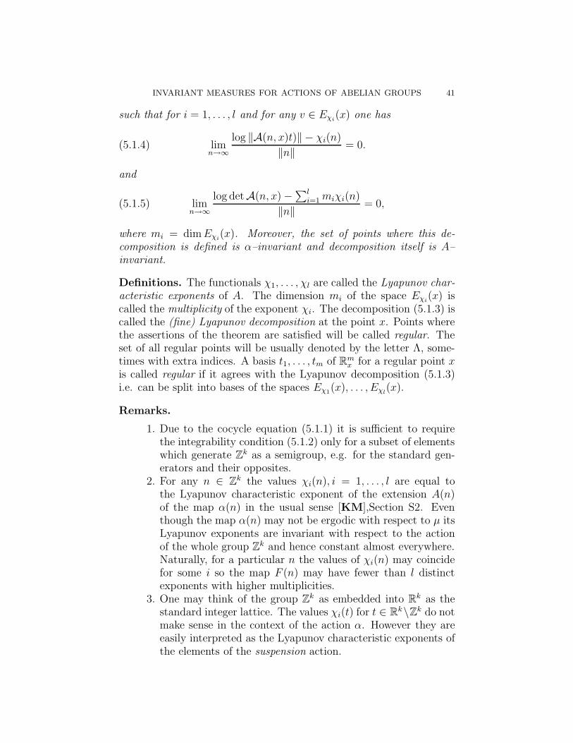
INVARIANT MEASURES FOR ACTIONS OF ABELIAN GROUPS 41
such that for i = 1, . . . , l and for any v ∈ Eχi(x) one has
(5.1.4) limn→∞
log ‖A(n, x)t)‖ − χi(n)
‖n‖= 0.
and
(5.1.5) limn→∞
log detA(n, x) −∑l
i=1miχi(n)
‖n‖= 0,
where mi = dimEχi(x). Moreover, the set of points where this de-
composition is defined is α–invariant and decomposition itself is A–invariant.
Definitions. The functionals χ1, . . . , χl are called the Lyapunov char-acteristic exponents of A. The dimension mi of the space Eχi
(x) iscalled the multiplicity of the exponent χi. The decomposition (5.1.3) iscalled the (fine) Lyapunov decomposition at the point x. Points wherethe assertions of the theorem are satisfied will be called regular. Theset of all regular points will be usually denoted by the letter Λ, some-times with extra indices. A basis t1, . . . , tm of Rm
x for a regular point xis called regular if it agrees with the Lyapunov decomposition (5.1.3)i.e. can be split into bases of the spaces Eχ1(x), . . . , Eχl
(x).
Remarks.
1. Due to the cocycle equation (5.1.1) it is sufficient to requirethe integrability condition (5.1.2) only for a subset of elementswhich generate Zk as a semigroup, e.g. for the standard gen-erators and their opposites.
2. For any n ∈ Zk the values χi(n), i = 1, . . . , l are equal tothe Lyapunov characteristic exponent of the extension A(n)of the map α(n) in the usual sense [KM],Section S2. Eventhough the map α(n) may not be ergodic with respect to µ itsLyapunov exponents are invariant with respect to the actionof the whole group Zk and hence constant almost everywhere.Naturally, for a particular n the values of χi(n) may coincidefor some i so the map F (n) may have fewer than l distinctexponents with higher multiplicities.
3. One may think of the group Zk as embedded into Rk as thestandard integer lattice. The values χi(t) for t ∈ Rk\Zk do notmake sense in the context of the action α. However they areeasily interpreted as the Lyapunov characteristic exponents ofthe elements of the suspension action.

42 BORIS KALININ AND ANATOLE KATOK
Theorem 5.1 can be easily deduced from the standard OseledetsMultiplicative ergodic theorem for linear extensions of a single measure–preserving transformation [O],[BKP] by a simple induction process.Namely, one first applies Oseledets theorem to the first generator ofthe Zk action. The Lyapunov decomposition for it is invariant underthe whole action so one can apply Oseledets theorem to the restrictionof the extension of the second generator to each element of the Lya-punov decomposition and so on. Once one obtained a decompositionfor which limits exist for multiples of all generators, existence of thelimits (5.1.4), (5.1.5) and the linearity of exponents follow easily fromthe cocycle relation (5.1.1).
Denote the standard scalar product in Rm by < ·, · >. Given ǫ >0 and a regular point x we will call the standard ǫ–Lyapunov scalarproduct (or metric) the scalar product < ·, · >x,ǫ in Rm
x defined asfollows:
For u, v ∈ Eχi(x), i = 1, . . . , l:
< u, v >x,ǫ=∑
n∈Zk
< A(n, x)u,A(n, x)v > exp(−2χi(n) − ǫ‖n‖),
where the series converges due to (5.1.4).For u ∈ Eχi
(x), v ∈ Eχj(x), i 6= j < u, v >x,ǫ= 0
We will usually omit the word “standard” and will call this scalarproduct ǫ–Lyapunov scalar product, or, if ǫ has been fixed and no confu-sion may appear, simply Lyapunov scalar product. The norm generatedby this scalar product will be called the (standard ǫ–) Lyapunov normand denoted by ‖ · ‖x,ǫ
By construction of the standard ǫ–Lyapunov norm one has for u ∈Eχi
(x),(5.1.6)exp(χi(n) − ǫ‖n‖)‖u‖x,ǫ ≤ ‖A(n, x)u)‖x,ǫ ≤ exp(χi(n) + ǫ‖n‖)‖u‖x,ǫ.
Notice that by definition ‖u‖x,ǫ ≥ m−1/2‖u‖.Denote for a δ > 0 by Λǫ,δ the following subset of the set of regular
points:
(5.1.7) Λǫ,δ = {x ∈ X : ∀u ∈ {x} ⊕ Rm, ‖u‖x,ǫ ≤ δ−1‖u‖}.
A real–valued function φ on X is called tempered at x (with respect tothe action α) if
limn→∞
φ(α(n, x))
n= 0.
It is easy to see that a tempered function can be estimated from aboveby a slowly changing function. Namely, let φ be tempered and let ǫ > 0.

INVARIANT MEASURES FOR ACTIONS OF ABELIAN GROUPS 43
We define
φǫ(x) = maxn∈Zk
(|φ(α(n, x))| − ǫ‖n‖).
Obviously φǫ(x) ≥ |φ(x)|. A simple calculation shows that φǫ indeedchanges slowly:
(5.1.8) φǫ(x) − ǫ‖n‖ ≤ φǫ(α(n, x)) ≤ φǫ(x) + ǫ‖n‖.
The following fact is proved in the same way as for k = 1 in [P],[BKP].
Proposition 5.1 (Temperedness of the Lyapunov metrics). Forany regular point x ∈ X any non-zero u ∈ Rm
x and any ǫ > 0 the
function log ‖u‖x,ǫ
‖u‖is tempered.
Two cocycles A and B over the same action α are called equivalentif there exists a function C : X → GL(m,R) such that
max{log ‖C‖, log ‖C−1‖}
is a tempered function and
B(n, x) = C−1(x)A(n, x)C(α(x, n)).
Equivalent cocycles have the same Lyapunov characteristic exponentswith the same multiplicities. The above proposition implies that anymeasurable coordinate change which takes the standard scalar productto the standard ǫ–Lyapunov scalar product is tempered. Thus anycocycle A satisfying (5.1.2) is equivalent to a block cocycle with mi×mi
diagonal blocks Ai(n, x), i = 1, . . . , l such that
‖Ai(n, x)‖ ≤ exp(χi(n)+ǫ‖n‖) and ‖A−1i (n, x)‖ ≥ exp(−χi(n)−ǫ‖n‖).
We will call any measurable coordinate change of this kind an ǫ–Lyapunov coordinate change an the resulting equivalent cocycle an ǫ–reduced cocycle.
5.2. Lyapunov hyperplanes and Weyl chambers. Now wecan generalize certain notions previously introduced in Sections 1.2.3and 1.3 for special cases.
The hyperplane kerχ ⊂ Rk, where χ is a non-zero Lyapunov expo-nent, is called a Lyapunov hyperplane. The subspace χ−1(−∞, 0) (corrχ−1(0,∞)) is called a negative (corr. positive) Lyapunov half-space. ALyapunov hyperplane L is called rational if L∩Zk is a lattice in L, to-tally irrational if L ∩ Zk = {0}, and partially irrational otherwise. Fork = 2 we will call Lyapunov hyperplanes Lyapunov lines. Naturally ,every Lyapunov line is either rational or totally irrational; in the lattercase we will call it simply irrational.

44 BORIS KALININ AND ANATOLE KATOK
A linear extension of an ergodic Zk action is called partially hyper-bolic if there is at least one non-zero Lyapunov exponent and hyperbolicif all Lyapunov exponents are different from zero.
A hyperbolic linear extension is called totally non–symplectic (TNS)if non of the Lyapunov exponents is proportional to another with thenegative coefficient of proportionality.
An element n ∈ Zk is called regular if n does not belong to any ofthe Lyapunov hyperplanes. A regular element for a hyperbolic linearextension of a Zk action is called hyperbolic. A Weyl chamber is aconnected component of the complement to the union of all Lyapunovhyperplanes.
Each Weyl chamber is an open convex polyhedral cone in Rk. Insidea Weyl chamber every non-zero Lyapunov exponent has a constant sign.Conversely, the locus of points in Rk for which each non-zero Lyapunovexponent has a particular sign is either empty or is a Weyl chamber.Thus any Weyl chamber can be characterized as a minimal non-emptyintersection of positive and negative Lyapunov half-spaces.
For a partially hyperbolic element n ∈ Zk and a regular point x weset
E+n (x) =
⊕
i:χi(n)>0
Eχi(x) and E−
n (x) =⊕
i:χi(n)<0
Eχi(x).
These subspaces are called correspondingly the expanding (or unsta-ble ) and the contracting (or stable) subspaces for n at the point x.Notice that for any n ∈ Zk if one takes in the definition of the stan-
dard ǫ–Lyapunov metric ǫ < ǫ0(n) = min |χi(n)|‖n‖
where the minimum is
taken over all exponents which do not vanish at n, then the extensionA(n) uniformly contracts the ǫ–standard Lyapunov metric in the con-tracting subspaces of all regular points and uniformly expands it in theexpanding subspaces of those points. By making an ǫ–Lyapunov coor-dinate change we obtain an equivalent cocycle generating an extensionB such that B(n) uniformly contracts the standard Euclidean metric inthe contracting subspaces of all regular points and uniformly expandsit in the expanding subspaces of those points.
By definition contracting and expanding subspaces are the samefor all elements in the same Weyl chamber. Any minimal non-zerointersection of expanding subspaces for various regular elements cor-responds to a positive Lyapunov half-space H and will be denoted byEH(x). It is equal to the sum of the subspaces Eχi
for those χi’s whichare positive on the subspace H . In other words, all these exponentsare proportional with positive proportionality coefficients. Thus forany Lyapunov half–space H one can find a uniquely defined Lyapunov
INVARIANT MEASURES FOR ACTIONS OF ABELIAN GROUPS 45
characteristic exponent χ(H) (called the bottom exponent for H) andpositive numbers 1 = c1(H) < c2(H) <, . . . , < cm(H)(H) such that
EH(x) =
m(H)⊕
i=1
Eci(H)χ(H).
Let us denote
EiH(x) =
m(H)⊕
j=i
Ecj(H)χ(H).
The nested sequence EH(x) = E1H(x) ⊃ E2
H(x) ⊃ · · · ⊃ Em(H)H (x) =
Ecm(H)(H)χ(H) is called the upper filtration of the space EH(x).Number all positive Lyapunov half–spaces by H1, . . . , Hs. We will
call the decomposition
Rmx =
s⊕
i=1
EHi(x)
the coarse Lyapunov decomposition at the point x. Extension A iscalled multiplicity–free if all Lyapunov exponents are simple and no twoof them are positively proportional. In other words, in the multiplicity–free case the elements of the coarse Lyapunov decomposition are one–dimensional.
5.3. Strongly hyperbolic extensions. In the case of multipleexponents it is convenient to count each exponent the number of timesequal to its multiplicity so that there are always exactly m exponents.Since this will not cause any confusion, from now on we will denoteexponents listed this way by χ1, . . . , χm, unless explicitly stated other-wise. This allows us to define the Lyapunov map ΨA : Rk → Rm byΨA = (χ1, . . . , χm). The Lyapunov map is defined up to a permutationof coordinates.
Thus the linear extension µ is hyperbolic if and only if Im ΨA doesnot lie in any coordinate hyperplane. We will call dim Ker ΨA thedefect of µ and denote it by d(A). Equivalently, d(A) is equal to the di-mension of the intersection of all Lyapunov hyperplanes. Furthermore,dim Im ΨA is called the rank of A and is denoted by r(A). Equivalently,r(A) is equal to the maximal number of linearly independent Lyapunovexponents.
Definition A hyperbolic linear extension A is called strongly hyperbolicif d(A) = 0, i.e. if the intersection of all Lyapunov hyperplanes consistsof the origin.

46 BORIS KALININ AND ANATOLE KATOK
Obviously, d(A) + r(A) = k and since r(A) ≤ m
k ≤ m+ d(A).
In particular, for any strongly hyperbolic measure
(5.3.1) k ≤ m.
5.4. Resonances. Let χ1, . . . , χl be the different Lyapunov expo-nents of an extension A as in Section 1.1.We will say that A possessesan essential resonance if the following two conditions hold:
(R1) There exist i ∈ {1, . . . , l} and non–negative integers s1, . . . , sl
such that
(5.4.1) χi =∑
j 6=i
sjχj
(R2) There exists a Weyl chamber W such that in W χi < 0 andχj < 0 for all j such that sj 6= 0.
If A does not possess any essential resonances we will call it essen-tially non-resonant. If in addition all exponents are simple (multiplicityone ) we will say that A is non–resonant.
Let x1, . . . , xl be negative numbers. We will call a relation of theform
(5.4.2) xi =∑
j 6=i
sjxj ,
where s1, . . . , sl are non–negative integers, a resonance relation betweenx1, . . . , xl. Notice that any given set of negative numbers may satisfyonly finitely many resonance relations.
Proposition 5.2. There exists an element n ∈ Zk ∩W such that
(1) The multiplicities of the Lyapunov exponents for the extensionA(n) are the same as for the extension A.
(2) Any resonance relation between the negative Lyapunov charac-teristic exponents of A(n) comes from an essential resonancefor A.
A proof of this statement is contained in the proof of [K1], Theorem4.4.

INVARIANT MEASURES FOR ACTIONS OF ABELIAN GROUPS 47
6. Normal forms and linearization of non-linear extensions
6.1. Extensions by non-linear contractions. We will be inter-ested later on in the way a smooth Zk action with a partially hyperbolicinvariant measure acts on the family of stable manifolds of its regularelement. This naturally leads us to the study of measurable extensionsof a measure–preserving transformation by diffeomorphisms preservingthe zero section with negative Lyapunov exponents for the derivativeat that section, as well as centralizers of such extensions.
Let as before (X,µ) be a probability Lebesgue space and α : Zk ×X → X be an ergodic action of the group Zk by measure–preservingtransformations of the space (X,µ). We will assume that an extensionΦ of α is defined in a neighborhood of the zero section, preserves thezero section and acts by C∞ diffeomorphisms in the fibers. In otherwords, Φ can be written in coordinates (x, t) ∈ X × Rm as
(6.1.1) Φ(n, x, t) = (α(n, x),F(n, x)(t)),
where F(n, 0) = 0 and F is C∞ in t.The derivatives in the t variable at the zero section which we will
denote simply by DF0(n, x) define a linear extension of α. We assumethat for some n0 ∈ Zk, DF0(n0, x) has negative characteristic expo-nents. We will also assume that all partial derivatives of all orders aretempered functions.
We will consider the following natural notion of equivalence for ex-tensions of the form (6.1.1). Namely, we will allow coordinate changeswhich are measurable in x, preserve each fiber Rm
x , fix the origin, areC∞ in each fiber and have tempered logarithm of all derivatives of allorders at the zero section. We will call such coordinate changes admis-sible. Our main purpose is to show that any extension can be broughtto a certain normal form by an admissible coordinate change. We willdo it by first considering the element F (n0). We will find a normalform for it and them describe the centralizer of that normal form. Thisdescription will show that the admissible coordinate change bringingF (n0) to its normal form also brings the whole extension F to a certainnormal form. The simplest kind of such a normal form is linear. Theobstacles to linearization of F (n0) via an admissible coordinate changeare resonance relations between the Lyapunov characteristic exponentsof the derivative at the zero section. Presence of such relations mightforce existence of certain non–linear resonance terms in the normalform.
6.2. Normal forms. The results of this sub–section represent oneof several natural “non–stationary” generalizations of well-known facts

48 BORIS KALININ AND ANATOLE KATOK
about normal forms of smooth contractions near a fixed point or aninvariant manifold which can be for example in [Be] and [BK]. An-other version of the non–stationary normal form theory for contractionsadapted to the study of uniformly hyperbolic dynamical systems is de-veloped in [GK] and [G]. The latter version is a crucial in the proofsof local differentiable rigidity both for actions of abelian groups [KS2],as well as higher rank Lie groups and their lattices [MQ].
Let (X,µ) be a probability Lebesgue space, f : X → X be ameasure–preserving transformation of (X,µ), not necessarily ergodic,U an open neighborhood of the origin in Rm and Φ : X×U → X×Rm
an extension of f satisfying assumptions corresponding those for Φ(n0)above. Namely, it preserves the zero section, is C∞ along the fibers, theLyapunov characteristic exponents for the linear extension defined bythe derivatives at zero section are constant almost everywhere and neg-ative and all higher derivatives are tempered functions. Let χi, . . . χl
be different Lyapunov characteristic exponents of the derivative ex-tension and m1, . . . , ml be their multiplicities. Consider all the res-onance relations (5.4.2) between the numbers χi, . . . χl. RepresentRm as the direct sum of the spaces Rmi , . . . ,Rml and let (t1, . . . , tl)be the corresponding coordinate representation of a vector t ∈ Rm.Let P : Rm → Rm; (t1, . . . , tl) 7→ (P1(t1, . . . , tl), . . . , Pl(t1, . . . , tl)) bea polynomial map preserving the origin. We will say that the mapP is of resonance type if it contains only such homogeneous termsin Pi(t1, . . . , tl) with degree of homogeneity sj in the coordinates oftj, i = 1, . . . , l for which the resonance relation χi =
∑j 6=i sjχj holds.
It is easy to see that polynomial maps of the resonance type with in-vertible derivative at the origin form a group. Since there are onlyfinitely many resonance relations between χ1, . . . , χl this is a finite–dimensional Lie group. We will denote this group by Gχ. In particular,if there are no resonance relations between the numbers χ1, . . . χl thenGχ = GL(m,R), the group of linear automorphisms of Rm.
Theorem 6.1 (non–stationary normal form for contractions). Thereexists an admissible coordinate change in X ×Rm which transforms Φto an extension Ψ of the following form
(6.2.1) Ψ(x, t) = (f(x),Px(t))
where for almost every x ∈ X, Px ∈ Gχ.
The proof of Theorem 6.1 follows one of the usual schemes in thenormal form theory. ( see, e.g. [KH, Section 6.6], for the local caseand [GK] for the uniformly hyperbolic nonstationary case). It includesthree steps:

INVARIANT MEASURES FOR ACTIONS OF ABELIAN GROUPS 49
Step 1 Finding a tempered formal coordinate change, i.e. the Taylorseries at the zero section for the desired coordinate change.
Step 2 Constructing a tempered smooth (C∞) coordinate change forwhich the formal power series found at Step 1 is the Taylorseries at the zero section
Step 3 The coordinate change constructed at Step 2 conjugates ourextension with an extension which is C∞ tangent to the deriv-ative extension. We show that any two tempered C∞ tangentcontracting extensions are conjugate via a C∞ tempered coor-dinate change C∞ tangent to identity
We will outline Step 1 since at that step the role played by res-onances becomes apparent. In particular it becomes clear that thenonuniform case is a more direct generalization of the local one andthe Lyapunov exponents play exactly the same role as the eigenvalues.In the uniform case considered in [GK] an extra narrow band conditionis required and not only resonance but also subresonance terms have tobe allowed in the normal form. Of course the proce paid for this sim-plification is that the dependence on the base point in the nonuniformnonstationary normal form is only measurable even if all the data aresmooth.
Steps 2 and 3 are very sismilar to the uniform nonstationary argu-ments in [GK] since the use of Lyapunov metrics essentially reducesour situation to the case of an extension by uniform contractions.
First we make a linear coordinate which brings the derivative atthe zero section to the block form as described at the end of Sec-tion 5.1. Denote the mi × mi, i = 1, . . . , l blocks thus obtained byΦ1(x), . . . ,Φl(x). Denote the coordinates corresponding this block formby t1, . . . , tl, where ti ∈ Rmi .
We will look inductively for successive jets of the desired coordi-nate change at the zero section to eliminate the non–resonance termsof higher and higher order.The base of the induction is the linear co-ordinate change described above. At the nth inductive step we startform the extension whose nth jets are polynomials of resonance type.We will find a coordinate change with the identity linear part and poly-nomial homogeneous non–linear part of degree n+ 1. Composing thiscoordinate change with the result from the previous steps would notchange the lower order terms. The ti component Cx(t1, . . . , tl) of thecoordinate change with degree of homogeneity sj in the coordinates oftj, j = 1 . . . , l satisfies the following functional equation
Φi(x)Cx(t1, . . . , tl) − Cf(x)(Φ1(x)t1, . . . ,Φl(x)tl) = Hx(t),
50 BORIS KALININ AND ANATOLE KATOK
where Hx(t) is a known function determined by the previous steps ofthe process. Let for t = (t1, . . . , tl), Φ(t) = (Φ1(t1), . . . ,Φl(tl)). Inthe non–resonance case we can solve this equation by one of the two“telescoping sums”: if
(6.2.2) χi >∑
sjχj ,
then(6.2.3)
Cx(t) =
∞∑
m=0
Φ−1i (x) . . .Φ−1
i (fm(x))Hfm(x)(Φ(fm(x)) . . .Φ(f(x))(Φ(x))(t)),
where the series in the right–hand part converges exponentially; if
(6.2.4) χi <∑
sjχj ,
then(6.2.5)
Cx(t) = −∞∑
m=1
Φi(f−1(x)) . . .Φi(f
−m(x))Hf−m(x)(Φ−1(f−m(x)) . . .Φ−1(f−1(x))(t)),
where again the series converges exponentially. Notice that the formercase holds for all but finitely many homogeneous terms. The resonanceterms of degree n + 1 do not change. at this and successive steps.However that they were likely to have changed at the previous steps.Thus, while the type of normal form is determined by the first jet (thederivative extension), coefficients of its nth jet depend on the (n−1)stjet of the original extension.
Theorem 6.2 (Centralizer for resonance maps). Let g be a non–singular (not necessarily measure–preserving) transformation of the space(X,µ) commuting with f , and Γ(x, t) = (g(x),Gx(t)) be an extensionof g by C∞ local diffeomorphisms preserving the zero section and com-muting with an extension Ψ of the form (6.2.1). Then for almost everyx ∈ X, Gx ∈ Gχ.
For certain applications it is useful to define another class of polyno-mial maps associated with a given set of Lyapunov exponents. As be-fore let P : Rm → Rm; (t1, . . . , tl) 7→ (P1(t1, . . . , tl), . . . , Pl(t1, . . . , tl))be a polynomial map preserving the origin. We will say that the mapP is of sub–resonance type if it has homogeneous terms in Pi(t1, . . . , tl)with degree of homogeneity sj in the coordinates of tj, i = 1, . . . , l onlyif
χi ≤∑
j 6=i
sjχj .

INVARIANT MEASURES FOR ACTIONS OF ABELIAN GROUPS 51
In other words, in addition to resonance terms we also allow termssatisfying the strict inequality (6.2.4). The product of two maps ofsub–resonance type is again a map of sub–resonance type; thus, as inthe case of resonance maps, polynomial maps of sub–resonance typewith invertible derivative at the origin form a group. It is larger thanGχ but still finite dimensional. We will denote this group by SRχ. Inparticular, if minχi > 2 maxχi, then SRχ = GL(m,R). Theorem 6.2has a counterpart for maps of sub–resonance type.
Theorem 6.3 (Centralizer for sub–resonance maps). Let Ψ be anextension of a measure–preserving transformation f ; (X,µ → (X,µ)of the following form
Ψ(x, t) = (f(x),Px(t)), where for almost every x ∈ X, Px ∈ SRχ.
Let g be a non–singular transformation of the space (X,µ) commutingwith f , and Γ(x, t) = (g(x),Gx(t)) be an extension of g by C∞ localdiffeomorphisms preserving the zero section and commuting with anextension Ψ . Then for almost every x ∈ X, Gx ∈ SRχ.
The proofs of theorems 6.2 and 6.3 are similar to the proof of The-orem 1.2 from [GK] with a proper allowance for non–uniformity of thesituation. Details will appear in a separate paper.
7. Pesin theory for Zk actions
7.1. Local Zk actions and rank restrictions.
7.1.1. Locally maximal sets. The main situation when the generalsetup described in the previous two sections arises is the extension of asmooth Zk action by derivatives. A somewhat more general semi-localsetup is as follows.
Let M be a differentiable manifold, U ⊂M an open set and Λ ⊂ Ua compact subset. Let f1, . . . , fk : U → M be commuting diffeomor-phic embeddings of class C1+ǫ for some ǫ > 0 preserving the set Λ.Obviously, the maps f1, . . . , fk restricted to the set Λ generate an ac-tion of the group Zk on Λ. Outside Λ the action of the whole groupZk may not be defined. We will call this situation a local Zk actionnear Λ. Our standard notation for a local action will be F so that forn = (n1, . . . , nk) ∈ Zk one has F (n1, . . . , nk) = fn1
1 ◦ · · · ◦ fnk
k . The setΛ is called a locally maximal set for the local action F if for some openset V ⊃ Λ the set Λ is the biggest invariant set contained in V , i.e.
Λ =⋂
n∈Zk
F (n)V.
Any such set V will be called a separating neighborhood for Λ.
52 BORIS KALININ AND ANATOLE KATOK
7.1.2. Lyapunov exponents and hyperbolic measures for local ac-tions. Let µ be a Borel probability F -invariant ergodic measure suchthat supp µ ⊂ Λ. Even though the tangent bundle TM or its restric-tion to Λ, TΛM may not be trivial, it is always trivial up to a setof measure zero. So the derivatives of the local action DF acting onTΛM generate a linear extension of F as described in Section 5. Differ-ent trivializations define cohomologous linear extensions ( see [KM])so various properties of this extensions discussed in Section 5 do notdepend on a particular choice of the trivialization. Accordingly we willattribute these properties to the action F itself. Thus we will speakof the Lyapunov characteristic exponents, hyperbolic measures, Weylchambers, etc of a local action.
In the smooth situation various feature of the structure of the deriv-ative extension are more of less directly reflected in the structure of the(non-linear) action itself. Accordingly we will associate the attributesof the derivative extension to the action and the measure. Notice thatcocycles associated to the derivative extension depend on a choice ofa measurable trivialization of the tangent bundle but cocycles corre-sponding to different trivializations are cohomologous. Thus Lyapunovexponents for the derivative cocycle with respect to an ergodic invari-ant measure are constant almost everywhere and thus are well definedas well as all notions derived form those exponents: Lyapunov hyper-planes, Weyl chambers, Lyapunov map, rank, defect, etc. We will thusspeak about Lyapunov exponents of a local action with respect to aninvariant measure, about partially hyperbolic, strongly hyperbolic andTNS (totally nonsymplectic) measures. In this case we will use thenotation Ψµ for the Lyapunov map, r(µ) for the rank and so on.
7.1.3. TNS actions. Cartan actions ([KKS]) of which the Z2 ac-tions of section 2.1 are the simplest examples are TNS. See [NT, Sec-tion 5] for a detailed discussion of TNS actions, in particular for specificexamples of such actions on Tori and nilmanifolds. Among algebraicAnosov actions discussed in Section 1.3 TNS actions appear only amongactions by automorphisms of tori and nilmanifolds, their finite affineextensions and suspensions. Most of the other interesting examples, arerelated in one way or another with semisimple Lie groups, and hencepossess at least a partial simplectic structure in certain transverse di-rections. Hence some Lyapunov exponents appear in pairs which differby the sign. See the description of standard Anosov actions in [KS1].
7.1.4. The rank restriction.

INVARIANT MEASURES FOR ACTIONS OF ABELIAN GROUPS 53
Proposition 7.1 ([K1]). If Im Ψµ intersects the positive octantRn
+ (and hence also the negative octant −Rn+) then the measure µ is
atomic.
Corollary 7.1. If µ is a hyperbolic measure for a local Zk ac-tion and k = dimM + d(µ), then µ is atomic. In particular, anystrongly hyperbolic ergodic invariant measure for a local Zk action ona k–dimensional manifold is atomic.
Proof. Obviously r(µ) = dimM so Im Ψµ = RdimM ⊃ RdimM+ �
Corollary 7.1 immediately implies that if a local Zk action on ann–dimensional manifold possesses a strongly hyperbolic non–atomicinvariant measure than
(7.1.1) k ≤ n− 1.
This inequality cannot be improved. In fact, for any n ≥ 2 there isa Zn−1 action on the n–dimensional torus Tn by hyperbolic automor-phisms for which Lebesgue measure is invariant and strongly hyper-bolic. A “surgery” described in [KL] allows to produce actions of Zn−1
with strongly hyperbolic absolutely continuous invariant measures oncertain n–dimensional manifolds other than torus. The rank of thesemeasures is equal to n− 1.
A certain feature of these examples holds in general.
Corollary 7.2. If µ is a non-atomic hyperbolic measure for a localZk action F and r(µ) = dimM − 1 then there exists a regular elementn ∈ Zk such that F (n) has exactly one positive Lyapunov exponent andthis exponent is simple.
Further results of [K1] show that in the low–dimensional situations,i.e. for n = 2 or 3 the only way for a non–atomic hyperbolic measureto violate (7.1.1) is to have elements in the Zk action with massive (inparticular, full measure) sets of fixed points. In the real–analytic casethis leads to the following conclusion:
Proposition 7.2 ([K1]). Any hyperbolic invariant measure for aneffective real– analytic action of Z2 on a compact (real–analytic) surfaceor an effective real– analytic action of Z3 on a compact (real–analytic)three–manifold is atomic.
7.2. Regular neighborhoods and regular sets. (See [BP] fora more detailed discussion in the rank one case.) Consider an ergodicinvariant measure µ for a local Zk action F . For µ–a.e. point x ∈ Λ wecan construct for any ǫ > 0 the ǫ–Lyapunov metric for the derivativeextension. Fix a sufficiently small ǫ > 0; typically it is sufficient to

54 BORIS KALININ AND ANATOLE KATOK
assume that ǫ is less than a quarter of the minimal difference betweentwo different Lyapunov exponents of the derivative extension. Thereare two types of regular neighborhoods for regular points in the senseof Section 5.1. The neighborhoods of the first kind are constructedby taking “boxes” i.e. products of balls in the Lyapunov metric ofa fixed sufficiently small size in the spaces Eχi
(x), i = 1, . . . , l andexponentiating these boxes by the exponential map of the referencesmooth Riemannian metric. The fine Lyapunov decomposition andthe ǫ–Lyapunov metric for any ǫ > 0 are continuous when restricted to
any set where ‖u‖x,ǫ
‖u‖is bounded. In particular the sets Λǫ,δ defined by
(5.1.7) are closed in this situation and the ǫ–Lyapunov metric and theregular neighborhoods are continuous on those sets. Such a neighbor-hood comes provided with a standard coordinate system, i.e. a smoothembedding of the standard box B in Rm into M . Continuity meanscontinuous dependence of this map from the base. point in a propertopology, typically, since we mostly deal with C∞ maps, the topologywill be the C∞ topology. Similarly to the rank one case [Br] it can beshown later that these structures are in fact Hoelder continuous.
The second type of regular neighborhoods is described in [KM],Theorem S.3.1. These neighborhoods are obtained by “truncating” theboxes in Lyapunov metric further to make their size changing slowlywith respect to the reference metric. In most situation any of the twotypes of regular neighborhoods may be used.
7.3. Stable and unstable manifolds. (See [BP].) Let us as-sume that µ is a hyperbolic measure. Specifying the discussion fromSection 5.2 to this case we obtain the coarse Lyapunov decompositionof TΛM :
TΛM =
s⊕
i=1
EHi(x).
Hadamard-Perron Theorem for Zk actions asserts that each elementof this decomposition as well as distributions obtained by the upperfiltration in such an element can be uniquely integrated to a familyof smooth submanifolds which possesses certain regularity propertiesaway from sets of small measure. More specifically fix a sufficientlysmall ǫ as before and let Λǫ = ∪δ>0Λǫ,δ.
Let E be a distribution from an upper filtration of the coarse Lya-punov decomposition and E ′ be the sum of the elements of the fineLyapunov decomposition which do not belong to E and x ∈ Λǫ. Inthe regular neighborhood R(x) of x of the first kind, there is a nat-ural product structure given by the exponential of the decomposition
INVARIANT MEASURES FOR ACTIONS OF ABELIAN GROUPS 55
TxM = E(x)⊕E ′(x). Then the local integral manifold E(x) ⊂ R(x) hasthe form expx graphφx, where φx : B(E(x)) → E ′(x). Here B(E(x))is the box around the origin in E(x) of fixed size in the Lyapunov met-ric used in the construction of the regular neighborhoods and φx is asmooth function (in fact, its degree of regularity is the same as for theaction F ), which vanishes at the origin together with its first differen-tial. Furthermore, if ‖DxF (n)‖x,ǫ < 1−ǫ, then F (n)(E(x)) ⊂ E(F (n)x)and F (n) contracts E(x). In fact, these manifolds can be obtained byconsidering upper filtrations for individual regular elements of the ac-tion constructing the corresponding families of integral manifolds andtaking their intersections. In the case E = EHi
one takes intersectionsof local stable manifolds for regular elements of the action.
The global integral manifold E(x) is defined as the smallest invariantset containing the local integral manifold E(x), i.e.
E(x) = ∪n∈ZkF (n)(E(F−n(x)).
Global integral manifolds are images of the Euclidean space undersmooth injective immersions.
As we mentioned before in the description of the regular sets Λǫ,δ
it is sufficient (and convenient) to fix a sufficiently small value of theparameter ǫ. This way we obtain a family of compact sets dependingon a single parameter which we will denote by θ. This parameterroughly can be thought as the “guaranteed size” of integral manifoldsfor the elements of the coarse Lyapunov decomposition and their upperfiltrations.
8. Rigidity of hyperbolic measures in dimension three: an
outline
The crucial feature of the argument in Section 2.2 was presenceof the critical direction such that the action along that direction wasisometric along the foliation W and sufficiently ergodic. If we wantto apply this type of arguments in more general situation we need tounderstand when a similar situation may appear.
In the case of algebraic actions discussed in Part I both the guidanceand the restrictions are provided by linear algebra. Now we will con-sider a situation which looks much more general from dynamical pointof view than our basic example of an action of Z2 on T3 by hyperbolicautomorphisms but whose geometric features are very similar.
8.1. Lyapunov Hoelder cocycle rigidity for TNS measures.
Let us consider an action α of Z2 by diffeomorphisms of a compactthree-dimensional manifold M . The key regularity assumption is C1+ǫ,

56 BORIS KALININ AND ANATOLE KATOK
for some ǫ > 0, but at the moment we can assume that the action is C∞.Consider an ergodic α-invariant measure µ such that all three Lyapunovexponents are different from zero and none of them are proportional. Inother words, the three Lyapunov lines (see Section 5.2) are all different.These lines divide R2 into six Weyl chambers. For a µ almost everypoint x ∈ M there exists a measurable α-invariant splitting of thetangent space TxM into three one-dimensional subspaces E1(x), E2(x),and E3(x) corresponding to three Lyapunov exponents. Each of thesedistributions as well as their pairwise sums are uniquely integrable to α-invariant families of smooth manifolds defined almost everywhere withrespect to the measure µ (See Section 7.3). While these distributions ingeneral are not continuous, they are Holder with respect to ǫ-Lyapunovmetrics defined in Section 5.1. Fix a smooth Riemannian metric on Mand let Ji(x, a) = log ||Dα(a)|Ei(x)||, i = 1, 2, 3. The function Ji areadditive one cocycles, i.e. Ji(x, a1 + a2) = Ji(x, a1) + Ji(α(a1)(x), a2).Naturally these cocycles are also Holder with respect to ǫ-Lyapunovmetrics. For these class of cocycles we can prove cohomological rigidity:for such a cocycle J one can find a function H , also satisfying a Holdercondition in a Lyapunov metric, and a homomorphism σ : Z2 → R
such thatJ(x, a) = σ(a) +H(α(a)(x)) −H(x).
8.2. Invariant affine structure on contracting manifolds.
Let W be one of the three families of one-dimensional invariant mani-folds. It turns out that there is a uniquely defined family of α-invariantsmooth affine parameters on these manifolds. This is a particular caseof the normal form results discussed in Section 6.2 (Theorems 6.2 and6.3 since in the case of a single exponent there are no resonance rela-tions. the proof is in fact more direct and simple than in gthe generalcase. The cocycle trivialization result described in the previous subsec-tion allows to normalize the affine parameters in such a way that theyare transformed by the transformation α(a) with the constant expan-sion or contraction coefficient expσ(a). Now pass to the suspension ofthe action α which we also denote by α. This action in the directionof the corresponding Lyapunov line preserves the normalized affine pa-rameters. From here on we can closely intimate the arguments for theautomorphisms of T3 from Section 2.2 exercising a certain care due tothe fact that this structure is only measurable.
8.3. Conditional measures and rigidity. Consider the systemof conditional measures on the leaves of W and identify a typical globalleaf with R using a point in the support of the conditional measure asthe origin and the length parameter normalized at that point. At
INVARIANT MEASURES FOR ACTIONS OF ABELIAN GROUPS 57
this moment it is important to keep in mind that the normalizations atdifferent (even typical) points of the same leaf need not agree. Howeverby Luzin Theorem type argument they do not differ more than a fixedamount on a set of large measure. Assumption (E) holds essentially bythe same reasons as in Section 2.2. The first part of the proof of the keyassertion (T ) which uses weak* compactness and Luzin theorem holdsessentially verbatim. Thus, the conditional measure on a typical leaf ofW is invariant (maybe up to a rescaling) with respect to an almost everytranslation. Again assuming that the conditionals are atomic impliesthat the every element of the action has zero entropy. In the case ofcontinuous conditional measures one sees again that the support of it isa closed subgroup of R, hence the whole R. The argument showing thatthe rescaling cocycle is identically equal to one again holds. Thus, theconditionals are Lebesgue with respect to the smooth invariant affineparameter, hence, absolutely continuous. After that simple argumentsusing Ledrappier’s converse [L] to the Pesin entropy formula [P] showthat the measure µ itself must be absolutely continuous. Thus theconclusion is the following very general counterpart of the statement(D) from section 2.2.
Theorem 8.1. Let µ be an ergodic invariant measure for a smoothaction of Z2 on a compact three-dimensional manifold M such thatall three Lyapunov characteristic exponents are different from zero andnone of them are proportional to each other. Then either µ is absolutelycontinuous or all elements of the action have zero entropy with respectto µ.
A detailed proof of this theorem will appear in a separate paper.An important corollary is the following result which to the bet of ourknowledge is the first instance in the differentiable dynamics in dimen-sion greater than one when global data (the homotopy class in ourcase) force existence of an invariant geometric structure for an actionof noncompact amenable group.
Theorem 8.2. Any Z2 action α on T3 which is homotopic to anaction α0 by hyperbolic automorphisms has an ergodic absolutely con-tinuous invariant measure.
Proof. There is a surjective continuous map φ : T3 → T3 suchthat
φ ◦ α = α0 ◦ φ.
This fact can be proven as follows. First, by a theorem of Franks ([KH,Theorem 2.6.1]) there is such a map homotopic to identity (call it φ(m))for each element α(m) for m ∈ Z2 \ {0} and it is unique. Uniqueness

58 BORIS KALININ AND ANATOLE KATOK
implies that the centralizer of any hyperbolic automorphism of a torusin the group of homeomorphisms of the torus coincides with its cen-tralizer in the group of automorphisms; in particular, this centralizercontains no more that one element in each homotopy class. Since forany m1,m2 ∈∈ Z2 \ {0} the map φ(m1)
−1 ◦ α(m2) ◦ φ(m1) commuteswith α0(m1) and is homotopic to α0(m2) = φ(m2)
−1 ◦ α(m2) ◦ φ(m2)we deduce that
φ(m1) = φ(m2).
In other words, the algebraic action α0 is a factor of the action α, or,equivalently α is an extension of α0.
Consider the set M of all Borel probability measures ν on T3 suchthat (φ)∗ν = λ, Lebesgue measure. The set M is convex, weak* com-pact and α invariant. Hence by Tychonoff theorem it contains an αinvariant measure. Since α0 is ergodic with respect to λ almost ev-ery ergodic component of an α-invariant measure ν ∈ M also belongsto M. Let µ be such an ergodic measure. We will show that it isabsolutely continuous.
Since (φ)∗µ = λ, for any m ∈ Z2, and since for each m ∈ Z2 eitherthe stable or unstable foiliation for α0(m) is one-dimensional, one has
hµ(α(m)) ≥ hλ(α0(m)) = | log max |χi(m)| |,
where χ1(m), χ2(m) and χ3(m) are eigenvalues of the matrix ρα(m).This implies in particular that the entropies hµ(α(m)) for all m ∈
Z2 \ {0} are uniformly bounded away from zero.In order to apply Theorem 8.1 we need to show that µ is a hyper-
bolic measure and that all three Lyapunov lines are different. Noticethat this is of course true for the Lebesgue measure with respect to α0;after all, this was the starting point of the argument in Section 2.2. Ifthere are no more than two Lyapunov lines for α then along at leastone of these lines at least two of the three Lyapunov exponents vanish.By Ruelle inequality [KM] this means that the entropy of the elementsof the suspension along that line vanishes. Since there are elements ofZ2 either on the line (if the latter is rational) or arbitrary close to it (ifit is irrational), there are nonzero elements of α with arbitrary smallentropy, a contradiction. �
References
[BKP] L. Barreira, A. Katok and Ya. Pesin, Non–uniformly hyperbolic dynamical
systems, monograph in preparation[BP] L. Barreira and Ya. Pesin, Lectures on Lyapunov exponents and smooth
ergodic theory, in Smooth ergodic theory and its applications, Proc. Symp.Pure Math, AMS, 2001.

INVARIANT MEASURES FOR ACTIONS OF ABELIAN GROUPS 59
[Be] G. R. Belitskii, Equivalence and normal forms of germs of smooth mappings,Russian Math. Surveys, 31 (1978), 107–177
[B] D. Berend, Multi-invariant sets on tori Trans. Amer. Math. Soc 280, (1983),509–533.
[BS] Z.I. Borevich and I.R. Shafarevich, Number Theory, Academic Press, NewYork, 1966.
[Br] M. Brin, Holder continuity of invariant distributions Appendix a to Lectures
on Lyapunov exponents and smooth ergodic theory, by L. Barreira and Ya.Pesin, in Smooth ergodic theory and its applications, Proc. Symp. PureMath, AMS, 2001.
[BK] I. U. Bronstein and A. Ja. Kopanskii, Smooth invariant manifolds and nor-
mal forms World scientific, 1994.[F] H. Furstenberg, Disjointness in ergodic theory, minimal sets, and a problem
in diophantine analysis, Math. Syst. Theory 1 (1967), 1–49[GS] E. Goetze and R. J. Spatzier, Smooth classification of Cartan actions of
higher rank semisimple Lie groups and their lattices, Ann. Math. 150 (1999),743–773
[GK] M. Guysinsky and A. Katok, Normal forms and invariant geometric struc-
tures for dynamical systems with invariant contracting foliations, Math. Res.Lett. 5 (1998), 149–163.
[G] M. Guysinsky The theory of nonstationary normal forms, Erg. Th. and Dy-nam. Syst. 21 (2001), to appear.
[H] H. Huyi, Some ergodic properties of commuting diffeomorphisms, Erg. Th.and Dynam. Syst. 13 (1993), 73–100
[KaK] B. Kalinin and A. Katok, Measurable rigidity and disjointness for Zk actions
by toral automorphisms, Erg. Th. and Dynam. Syst. , to appear.[K1] A. Katok, Hyperbolic measures and commuting maps in low dimension, Dis-
crete and cont. Dyn. Syst. 2 (1996), 397–411[K2] A. Katok, An introduction to rigidity of higher rank abelian group actions in
Ergodic theory, geometric rigidity and number theory , Proc of the Specialyear at the Newton Institute, Springer Verlag, to appear.
[KH] A. Katok and B. Hasselblatt, Introduction to the modern theory of dynamical
systems, Cambridge University Press, 1995.[KKS] A. Katok, S. Katok and K. Schmidt, Rigidity of measurable structure for Zd
actions by automorphisms of a torus, preprint, 2000.[KK] A. Katok and S. Katok, Higher cohomology for abelian groups of toral auto-
morphisms, Erg. Th. and Dynam. Syst. 15 (1995), 569–592[KL] A. Katok and J. Lewis, Global rigidity results for lattice actions on tori
and new examples of volume–preserving actions, Israel J. Math. 93 (1996),253–280
[KM] A. Katok and L. Mendoza, Dynamical systems with nonuniformly hyperbolic
behavior, Supplement to “Introduction to the modern theory of dynamicalsystems” (A. Katok and B. Hasselblatt) 1995, 659–700
[KNT] A. Katok, V. Nitica and A. Torok, Nonabelian Cohomology of Abelian
Anosov Actions,Erg. Th. and Dynam. Syst. 20 (2000), 259–288[KSch] A. Katok and K. Schmidt, The cohomology of expansive Zd actions by au-
tomorphisms of compact abelian groups Pacific J. Math 170 (1995) 105–142

60 BORIS KALININ AND ANATOLE KATOK
[KS1] A. Katok and R. J. Spatzier, First cohomology of Anosov actions of higher
rank Abelian groups and applications to rigidity, Publ. Math. IHES 79
(1994), 131–156[KS2] A. Katok and R. J. Spatzier, Differential Rigidity of Anosov Actions of
Higher Rank Abelian Groups and Algebraic Lattice Actions, Proc. SteklovInst. Math 216, (1997), 292–319
[KS3] A. Katok and R. J. Spatzier, Invariant Measures for Higher Rank Hyperbolic
Abelian Actions, Erg. Th. and Dynam. Syst. 16 (1996), 751–778[KS4] A. Katok and R. J. Spatzier, Corrections to “Invariant measures for higher
rank hyperbolic abelian actions”, Erg. Th. and Dynam. Syst. 18, (1998),503-507.
[Kat] I. Katznelson, Ergodic automorphisms of Tn are Bernoulli shifts, Israel J.Math 10, (1971), 186-195
[L] F. Ledrappier, Proprietes ergodiques des measures de Sinai, Publ. Math.IHES 59 (1984), 163–188
[MQ] G. Margulis and N. Qian, Local rigidity of weakly hyperbolic actions of higher
rank real Lie groups and their lattices, Erg. Th. and Dynam. Syst. 21 (2001),to appear
[NT] V. Nitica and A. Torok, On the cohomology of Anosov actions in Ergodictheory, geometric rigidity and number theory , Proc of the Special year atthe Newton Institute, Springer Verlag, to appear.
[O] V. I. Oseledets, A multiplicative ergodic theorem. Liapunov characteristic
numbers for dynamical systems, Trans. Moscow math. Soc 19 (1968), 197–221
[P] Y. Pesin, Characteristic exponents and smooth ergodic theory, Russian MathSurveys 32 (1977), 55–114
[R] V. A. Rohklin, On the fundamental ideas of measure theory, A.M.S. Transl.(1), 10 (1962), 1–52
[R] D. Rudolph, ×2 and ×3 invariant measures and entropy, Ergod. Th. andDynam. Syst. 10 (1990), 395–406
[S] A. Starkov, First cohomology group, mixing and minimal sets of commutative
group of algebraic action on torus, J. Math. Sci (New York) 95, (1999),2576–2582.
University of Michigan, Ann Arbor, MI
E-mail address : [email protected]
The Pennsylvania State University, University Park, PA
E-mail address : katok [email protected]


![COMPUTABLE ABELIAN GROUPS - Massey Universityamelniko/survey.pdf · COMPUTABLE ABELIAN GROUPS 5 standard references for pure abelian group theory are Fuchs [44, 45] and Kaplansky](https://img.dokumen.tips/doc/110x75/5f0639277e708231d416ea0e/computable-abelian-groups-massey-university-amelnikosurveypdf-computable-abelian.jpg)