Embed Size (px)
Citation preview

Invariance principle on the slice
Y. Filmus, E. Mossel, G. Kindler, K. Wimmer
30 May 2016

1 The result
2 Fourier analysis on the slice
3 The proof
4 Summary

Constant-weight vectorsfool low-degree polynomials∗

In more detail...
Suppose P is a suitable low-degree polynomial.
If (X1, . . . ,Xn) ∼ {0, 1}n and (Y1, . . . ,Yn) ∼( [n]n/2
)then
P(X1, . . . ,Xn) ≈ P(Y1, . . . ,Yn).

In more detail...
Suppose P is a suitable low-degree polynomial.
If (X1, . . . ,Xn) ∼ {0, 1}n and (Y1, . . . ,Yn) ∼( [n]n/2
)then
P(X1, . . . ,Xn) ≈ P(Y1, . . . ,Yn).

Unsuitable polynomials
Goal
P(~X ) ≈ P( ~Y ) where ~X ∼ {0, 1}n, ~Y ∼( [n]n/2
)
Obstructions
x1 + · · ·+ xn − n/2
(x1 + · · ·+ xn − n/2)x1
x1(1− n/2) + (x2 + · · ·+ xn)x1

Unsuitable polynomials
Goal
P(~X ) ≈ P( ~Y ) where ~X ∼ {0, 1}n, ~Y ∼( [n]n/2
)Obstructions
x1 + · · ·+ xn − n/2
(x1 + · · ·+ xn − n/2)x1
x1(1− n/2) + (x2 + · · ·+ xn)x1

Unsuitable polynomials
Goal
P(~X ) ≈ P( ~Y ) where ~X ∼ {0, 1}n, ~Y ∼( [n]n/2
)Obstructions
x1 + · · ·+ xn − n/2
(x1 + · · ·+ xn − n/2)x1
x1(1− n/2) + (x2 + · · ·+ xn)x1

Unsuitable polynomials
Goal
P(~X ) ≈ P( ~Y ) where ~X ∼ {0, 1}n, ~Y ∼( [n]n/2
)Obstructions
x1 + · · ·+ xn − n/2
(x1 + · · ·+ xn − n/2)x1
x1(1− n/2) + (x2 + · · ·+ xn)x1

Suitable polynomials
Definition
A polynomial P is harmonic if
n∑i=1
∂P
∂xi= 0.
Examples
x1 − x2(x1 − x2)(x3 − x4)
Theorem (Dunkl)
Every function on( [n]n/2
)has unique representation as
harmonic multilinear polynomial of degree ≤ n/2.

Suitable polynomials
Definition
A polynomial P is harmonic if
n∑i=1
∂P
∂xi= 0.
Examples
x1 − x2
(x1 − x2)(x3 − x4)
Theorem (Dunkl)
Every function on( [n]n/2
)has unique representation as
harmonic multilinear polynomial of degree ≤ n/2.

Suitable polynomials
Definition
A polynomial P is harmonic if
n∑i=1
∂P
∂xi= 0.
Examples
x1 − x2(x1 − x2)(x3 − x4)
Theorem (Dunkl)
Every function on( [n]n/2
)has unique representation as
harmonic multilinear polynomial of degree ≤ n/2.

Suitable polynomials
Definition
A polynomial P is harmonic if
n∑i=1
∂P
∂xi= 0.
Examples
x1 − x2(x1 − x2)(x3 − x4)
Theorem (Dunkl)
Every function on( [n]n/2
)has unique representation as
harmonic multilinear polynomial of degree ≤ n/2.

Formal statement
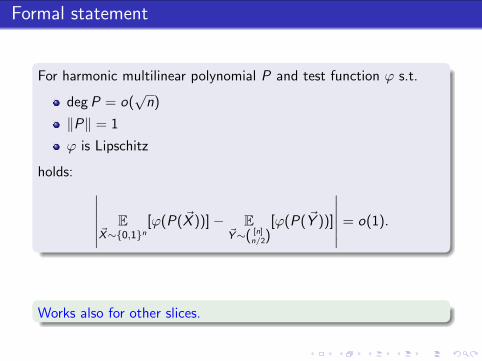
For harmonic multilinear polynomial P and test function ϕ s.t.
degP = o(√n)
‖P‖ = 1
ϕ is Lipschitz
holds: ∣∣∣∣∣∣ E~X∼{0,1}n
[ϕ(P(~X ))]− E~Y∼( [n]
n/2)[ϕ(P( ~Y ))]
∣∣∣∣∣∣ = o(1).
Works also for other slices.
Formal statement
For harmonic multilinear polynomial P and test function ϕ s.t.
degP = o(√n)
‖P‖ = 1
ϕ is Lipschitz
holds: ∣∣∣∣∣∣ E~X∼{0,1}n
[ϕ(P(~X ))]− E~Y∼( [n]
n/2)[ϕ(P( ~Y ))]
∣∣∣∣∣∣ = o(1).
Works also for other slices.

Consequences
Results for {0, 1}n proved using classical invariance principlegeneralize (almost) immediately to the slice.
Some examples
Majority is Stablest for the slice.
Bourgain’s tail bound for the slice.
Kindler–Safra theorem for the slice.

Consequences
Results for {0, 1}n proved using classical invariance principlegeneralize (almost) immediately to the slice.
Some examples
Majority is Stablest for the slice.
Bourgain’s tail bound for the slice.
Kindler–Safra theorem for the slice.

Consequences
Results for {0, 1}n proved using classical invariance principlegeneralize (almost) immediately to the slice.
Some examples
Majority is Stablest for the slice.
Bourgain’s tail bound for the slice.
Kindler–Safra theorem for the slice.

Consequences
Results for {0, 1}n proved using classical invariance principlegeneralize (almost) immediately to the slice.
Some examples
Majority is Stablest for the slice.
Bourgain’s tail bound for the slice.
Kindler–Safra theorem for the slice.

1 The result
2 Fourier analysis on the slice
3 The proof
4 Summary

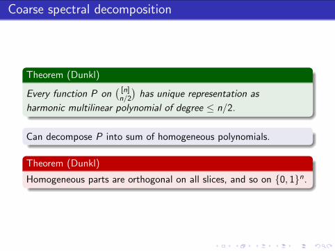
Coarse spectral decomposition
Theorem (Dunkl)
Every function P on( [n]n/2
)has unique representation as
harmonic multilinear polynomial of degree ≤ n/2.
Can decompose P into sum of homogeneous polynomials.
Theorem (Dunkl)
Homogeneous parts are orthogonal on all slices, and so on {0, 1}n.

Coarse spectral decomposition
Theorem (Dunkl)
Every function P on( [n]n/2
)has unique representation as
harmonic multilinear polynomial of degree ≤ n/2.
Can decompose P into sum of homogeneous polynomials.
Theorem (Dunkl)
Homogeneous parts are orthogonal on all slices, and so on {0, 1}n.
Coarse spectral decomposition
Theorem (Dunkl)
Every function P on( [n]n/2
)has unique representation as
harmonic multilinear polynomial of degree ≤ n/2.
Can decompose P into sum of homogeneous polynomials.
Theorem (Dunkl)
Homogeneous parts are orthogonal on all slices, and so on {0, 1}n.

L2 invariance
Theorem (F)
If a harmonic multilinear polynomial P has low degree then
L2 norm of P on( [n]n/2
)≈ L2 norm of P on {0, 1}n.
Prerequisite for full invariance principle.

L2 invariance
Theorem (F)
If a harmonic multilinear polynomial P has low degree then
L2 norm of P on( [n]n/2
)≈ L2 norm of P on {0, 1}n.
Prerequisite for full invariance principle.

Fourier basis for the slice
Srinivasan and F (independently) constructed an explicitorthogonal basis for the slice.
F used basis to reprove Wimmer’s junta theorem for the slice.
Basis isn’t needed to prove the invariance principle.

Fourier basis for the slice
Srinivasan and F (independently) constructed an explicitorthogonal basis for the slice.
F used basis to reprove Wimmer’s junta theorem for the slice.
Basis isn’t needed to prove the invariance principle.

Fourier basis for the slice
Srinivasan and F (independently) constructed an explicitorthogonal basis for the slice.
F used basis to reprove Wimmer’s junta theorem for the slice.
Basis isn’t needed to prove the invariance principle.

1 The result
2 Fourier analysis on the slice
3 The proof
4 Summary

Classical proof
Classical invariance principle (MOO)
Suitable low-degree polynomials behave similarlyon input {−1, 1}n and on input N(0, 1)n.
The proof
Replace one by one the {−1, 1} variables with N(0, 1) variablesand bound the error.
Our case
Strategy fails since coordinates of( [n]n/2
)are not independent!

Our proof(s)
Let P be a suitable low-degree polynomial on( [n]n/2
).
Dist. of P doesn’t change too much if we flip a coordinate.
Hence dist. of P on( [n]n/2
)is similar to its dist. on
( [n]n/2±t
).
and so similar to its distribution on( [n]n/2−t≤·≤n/2+t
).
Hence dist. of P on( [n]n/2
)is similar to its dist. on {0, 1}n.

1 The result
2 Fourier analysis on the slice
3 The proof
4 Summary

Recap
Constant-weight vectors foollow-degree harmonic multilinear polys

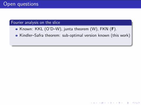
Open questions
Fourier analysis on the slice
Known: KKL (O’D–W), junta theorem (W), FKN (F).
Kindler–Safra theorem: sub-optimal version known (this work)
Linearity testing: some versions known (DDGKS, Tal)
Other domains
Association schemes (e.g. Grassmann)
Non-abelian groups (e.g. Sn)
Multislice
Applications
Suggestions welcome!

Thanks!

Fourier basis for the slice
Setup
A slice([n]k
).
Basis elements
For every ` ≤ min(k , n − k) and b1 < · · · < b` ≤ n:
χb1,...,b` =∑′
a1,...,a`
(xa1 − xb1) · · · (xa` − xb`),
where:
a1, b1, . . . , a`, b` all distinct.
a1 < b1, . . . , a` < b`.
Properties(n`
)−( n`−1)
basis elements at level `.
Basis is orthogonal.
Explicit formula for norm of χb1,...,b` .

Fourier basis for the slice
Setup
A slice([n]k
).
Basis elements
For every ` ≤ min(k , n − k) and b1 < · · · < b` ≤ n:
χb1,...,b` =∑′
a1,...,a`
(xa1 − xb1) · · · (xa` − xb`),
where:
a1, b1, . . . , a`, b` all distinct.
a1 < b1, . . . , a` < b`.
Only consider b1, . . . , b` for which sum is non-zero.
Properties(n`
)−( n`−1)
basis elements at level `.
Basis is orthogonal.
Explicit formula for norm of χb1,...,b` .

Fourier basis for the slice
Basis elements
For every ` ≤ min(k , n − k) and b1 < · · · < b` ≤ n:
χb1,...,b` =∑′
a1,...,a`
(xa1 − xb1) · · · (xa` − xb`),
where:
a1, b1, . . . , a`, b` all distinct.
a1 < b1, . . . , a` < b`.
Properties(n`
)−( n`−1)
basis elements at level `.
Basis is orthogonal.
Explicit formula for norm of χb1,...,b` .