Embed Size (px)
Citation preview
Introduction to XAS Theory
Bruce [email protected]
http://feff.phys.washington.edu/~ravel/
Version 0.1
September 11, 2002
Abstract
This is a document contains the presentation materials for a seminar entitled Introduction toXAS Theory. This file is suitable for presentation directly from a computer or for printing ontotransparency sheets.
Bruce [email protected]://feff.phys.washington.edu/˜ravel/
This document is copyright c© 2002 Bruce Ravel.
This document is distributed under the GNU Free Document License (FDL).
Permission is granted to make and distribute verbatim copies of this manual provided the copyright notice andthis permission notice are preserved on all copies.
Permission is granted to copy and distribute modified versions of this manual under the conditions for verbatimcopying, provided that the entire resulting derived work is distributed under the terms of a permission noticeidentical to this one and that it is distributed as transparent copy as defined in the FDL.
Permission is granted to copy and distribute translations of this manual into another language, under the aboveconditions for modified versions, except that this permission notice may be stated in a translation approved bythe author.
Table of Contents
Introduction to the theory . . . . . . . . . . . . . . . . . . . . . . . . . . . . . . . . . . . . . . . . . . . . . . . . . . . . . . . . . . . . . . . . . . . . . . . . . . . . . . . . . . . . . . . . . . . . . . . . . . . . 1EXAFS data . . . . . . . . . . . . . . . . . . . . . . . . . . . . . . . . . . . . . . . . . . . . . . . . . . . . . . . . . . . . . . . . . . . . . . . . . . . . . . . . . . . . . . . . . . . . . . . . . . . . . . . . . . . . . . . . . . 1A Heuristic Picture of EXAFS . . . . . . . . . . . . . . . . . . . . . . . . . . . . . . . . . . . . . . . . . . . . . . . . . . . . . . . . . . . . . . . . . . . . . . . . . . . . . . . . . . . . . . . . . . . . . . . . . 2Fermi’s Golden Rule . . . . . . . . . . . . . . . . . . . . . . . . . . . . . . . . . . . . . . . . . . . . . . . . . . . . . . . . . . . . . . . . . . . . . . . . . . . . . . . . . . . . . . . . . . . . . . . . . . . . . . . . . 3Motivating the multiple scattering expansion . . . . . . . . . . . . . . . . . . . . . . . . . . . . . . . . . . . . . . . . . . . . . . . . . . . . . . . . . . . . . . . . . . . . . . . . . . . . . . . . 4Paths and clusters: FCC copper . . . . . . . . . . . . . . . . . . . . . . . . . . . . . . . . . . . . . . . . . . . . . . . . . . . . . . . . . . . . . . . . . . . . . . . . . . . . . . . . . . . . . . . . . . . . . . 5The first path in FCC copper . . . . . . . . . . . . . . . . . . . . . . . . . . . . . . . . . . . . . . . . . . . . . . . . . . . . . . . . . . . . . . . . . . . . . . . . . . . . . . . . . . . . . . . . . . . . . . . . . 6The second path in FCC copper . . . . . . . . . . . . . . . . . . . . . . . . . . . . . . . . . . . . . . . . . . . . . . . . . . . . . . . . . . . . . . . . . . . . . . . . . . . . . . . . . . . . . . . . . . . . . . 7The third path in FCC copper . . . . . . . . . . . . . . . . . . . . . . . . . . . . . . . . . . . . . . . . . . . . . . . . . . . . . . . . . . . . . . . . . . . . . . . . . . . . . . . . . . . . . . . . . . . . . . . . 8The fourth path FCC copper . . . . . . . . . . . . . . . . . . . . . . . . . . . . . . . . . . . . . . . . . . . . . . . . . . . . . . . . . . . . . . . . . . . . . . . . . . . . . . . . . . . . . . . . . . . . . . . . . 9The fifth path in FCC copper . . . . . . . . . . . . . . . . . . . . . . . . . . . . . . . . . . . . . . . . . . . . . . . . . . . . . . . . . . . . . . . . . . . . . . . . . . . . . . . . . . . . . . . . . . . . . . . 10Selecting the important paths . . . . . . . . . . . . . . . . . . . . . . . . . . . . . . . . . . . . . . . . . . . . . . . . . . . . . . . . . . . . . . . . . . . . . . . . . . . . . . . . . . . . . . . . . . . . . . 11
Preparing input data for FEFF . . . . . . . . . . . . . . . . . . . . . . . . . . . . . . . . . . . . . . . . . . . . . . . . . . . . . . . . . . . . . . . . . . . . . . . . . . . . . . . . . . . . . . . . . . . . . . . 12The information needed by FEFF . . . . . . . . . . . . . . . . . . . . . . . . . . . . . . . . . . . . . . . . . . . . . . . . . . . . . . . . . . . . . . . . . . . . . . . . . . . . . . . . . . . . . . . . . . . 12A FEFF input file . . . . . . . . . . . . . . . . . . . . . . . . . . . . . . . . . . . . . . . . . . . . . . . . . . . . . . . . . . . . . . . . . . . . . . . . . . . . . . . . . . . . . . . . . . . . . . . . . . . . . . . . . . . . 13A few more details about FEFF’s input file . . . . . . . . . . . . . . . . . . . . . . . . . . . . . . . . . . . . . . . . . . . . . . . . . . . . . . . . . . . . . . . . . . . . . . . . . . . . . . . . . . 14Using Atoms to prepare the FEFF input file . . . . . . . . . . . . . . . . . . . . . . . . . . . . . . . . . . . . . . . . . . . . . . . . . . . . . . . . . . . . . . . . . . . . . . . . . . . . . . . . . 15Preparing the FEFF input file for non-crystalline materials . . . . . . . . . . . . . . . . . . . . . . . . . . . . . . . . . . . . . . . . . . . . . . . . . . . . . . . . . . . . . . . . . 16
Running FEFF on your computer . . . . . . . . . . . . . . . . . . . . . . . . . . . . . . . . . . . . . . . . . . . . . . . . . . . . . . . . . . . . . . . . . . . . . . . . . . . . . . . . . . . . . . . . . . . . 17Running FEFF . . . . . . . . . . . . . . . . . . . . . . . . . . . . . . . . . . . . . . . . . . . . . . . . . . . . . . . . . . . . . . . . . . . . . . . . . . . . . . . . . . . . . . . . . . . . . . . . . . . . . . . . . . . . . . 17FEFF’s output files . . . . . . . . . . . . . . . . . . . . . . . . . . . . . . . . . . . . . . . . . . . . . . . . . . . . . . . . . . . . . . . . . . . . . . . . . . . . . . . . . . . . . . . . . . . . . . . . . . . . . . . . . . 18The path files and the EXAFS equation . . . . . . . . . . . . . . . . . . . . . . . . . . . . . . . . . . . . . . . . . . . . . . . . . . . . . . . . . . . . . . . . . . . . . . . . . . . . . . . . . . . . . 19Fitting data as a sum of paths . . . . . . . . . . . . . . . . . . . . . . . . . . . . . . . . . . . . . . . . . . . . . . . . . . . . . . . . . . . . . . . . . . . . . . . . . . . . . . . . . . . . . . . . . . . . . . . 20Paths at the fourth shell distance . . . . . . . . . . . . . . . . . . . . . . . . . . . . . . . . . . . . . . . . . . . . . . . . . . . . . . . . . . . . . . . . . . . . . . . . . . . . . . . . . . . . . . . . . . . 21Fitting to the fourth shell distance . . . . . . . . . . . . . . . . . . . . . . . . . . . . . . . . . . . . . . . . . . . . . . . . . . . . . . . . . . . . . . . . . . . . . . . . . . . . . . . . . . . . . . . . . . 22
Why theoretical standards are important . . . . . . . . . . . . . . . . . . . . . . . . . . . . . . . . . . . . . . . . . . . . . . . . . . . . . . . . . . . . . . . . . . . . . . . . . . . . . . . . . . . . 23The need for theoretical standards: overlapping shells . . . . . . . . . . . . . . . . . . . . . . . . . . . . . . . . . . . . . . . . . . . . . . . . . . . . . . . . . . . . . . . . . . . . . . 23Three-body correlations . . . . . . . . . . . . . . . . . . . . . . . . . . . . . . . . . . . . . . . . . . . . . . . . . . . . . . . . . . . . . . . . . . . . . . . . . . . . . . . . . . . . . . . . . . . . . . . . . . . . 24The effect of polarization . . . . . . . . . . . . . . . . . . . . . . . . . . . . . . . . . . . . . . . . . . . . . . . . . . . . . . . . . . . . . . . . . . . . . . . . . . . . . . . . . . . . . . . . . . . . . . . . . . . 25Other examples . . . . . . . . . . . . . . . . . . . . . . . . . . . . . . . . . . . . . . . . . . . . . . . . . . . . . . . . . . . . . . . . . . . . . . . . . . . . . . . . . . . . . . . . . . . . . . . . . . . . . . . . . . . . . 26
References and URLs . . . . . . . . . . . . . . . . . . . . . . . . . . . . . . . . . . . . . . . . . . . . . . . . . . . . . . . . . . . . . . . . . . . . . . . . . . . . . . . . . . . . . . . . . . . . . . . . . . . . . . . . . 27XAFS theory links on the web . . . . . . . . . . . . . . . . . . . . . . . . . . . . . . . . . . . . . . . . . . . . . . . . . . . . . . . . . . . . . . . . . . . . . . . . . . . . . . . . . . . . . . . . . . . . . . . 27FEFF literature references . . . . . . . . . . . . . . . . . . . . . . . . . . . . . . . . . . . . . . . . . . . . . . . . . . . . . . . . . . . . . . . . . . . . . . . . . . . . . . . . . . . . . . . . . . . . . . . . . . 28
Introduction to XAS Theory, c© 2002 Bruce Ravel Page i
Introduction to the theory 1.1
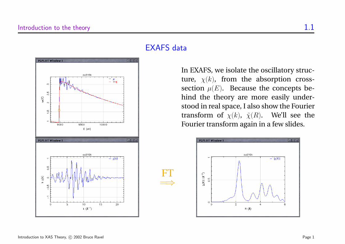
EXAFS data
In EXAFS, we isolate the oscillatory struc-ture, χ(k), from the absorption cross-section µ(E). Because the concepts be-hind the theory are more easily under-stood in real space, I also show the Fouriertransform of χ(k), χ(R). We’ll see theFourier transform again in a few slides.
FT=⇒
Introduction to XAS Theory, c© 2002 Bruce Ravel Page 1
Introduction to the theory 1.2
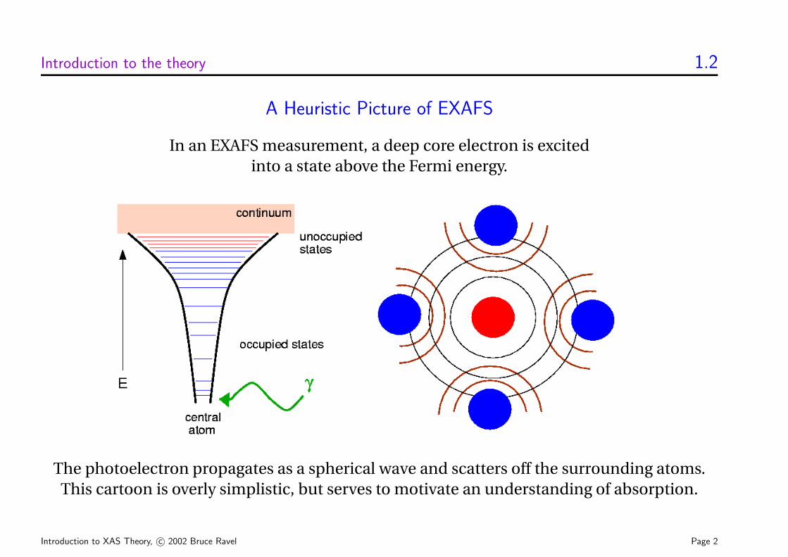
A Heuristic Picture of EXAFS
In an EXAFS measurement, a deep core electron is excitedinto a state above the Fermi energy.
The photoelectron propagates as a spherical wave and scatters off the surrounding atoms.This cartoon is overly simplistic, but serves to motivate an understanding of absorption.
Introduction to XAS Theory, c© 2002 Bruce Ravel Page 2
Introduction to the theory 1.3
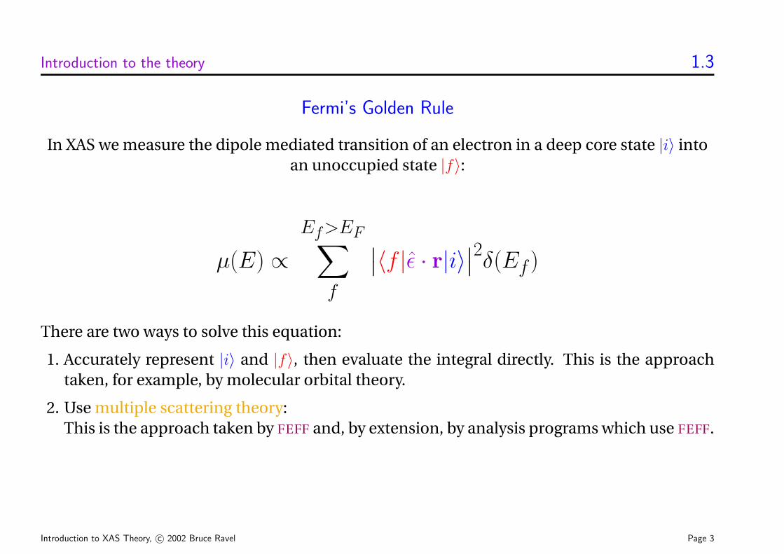
Fermi’s Golden Rule
In XAS we measure the dipole mediated transition of an electron in a deep core state |i〉 intoan unoccupied state |f〉:
µ(E) ∝Ef>EF∑
f
∣∣〈f |ε · r|i〉∣∣2δ(Ef )
There are two ways to solve this equation:
1. Accurately represent |i〉 and |f〉, then evaluate the integral directly. This is the approachtaken, for example, by molecular orbital theory.
2. Use multiple scattering theory:This is the approach taken by FEFF and, by extension, by analysis programs which use FEFF.
Introduction to XAS Theory, c© 2002 Bruce Ravel Page 3
Introduction to the theory 1.4
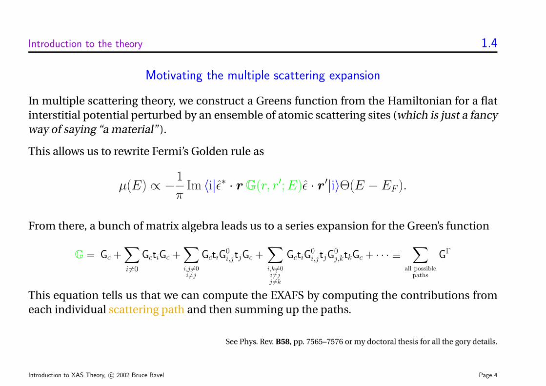
Motivating the multiple scattering expansion
In multiple scattering theory, we construct a Greens function from the Hamiltonian for a flatinterstitial potential perturbed by an ensemble of atomic scattering sites (which is just a fancyway of saying “a material” ).
This allows us to rewrite Fermi’s Golden rule as
µ(E) ∝ −1
πIm 〈i|ε∗ · rG(r, r′;E)ε · r′|i〉Θ(E − EF ).
From there, a bunch of matrix algebra leads us to a series expansion for the Green’s function
G = Gc +∑i 6=0
GctiGc +∑i,j 6=0i 6=j
GctiG0i,jtjGc +
∑i,k 6=0i 6=jj 6=k
GctiG0i,jtjG
0j,ktkGc + · · · ≡
∑all possible
paths
GΓ
This equation tells us that we can compute the EXAFS by computing the contributions fromeach individual scattering path and then summing up the paths.
See Phys. Rev. B58, pp. 7565–7576 or my doctoral thesis for all the gory details.
Introduction to XAS Theory, c© 2002 Bruce Ravel Page 4
Introduction to the theory 1.5
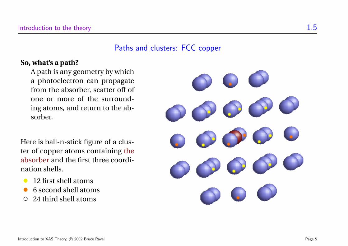
Paths and clusters: FCC copper
So, what’s a path?A path is any geometry by whicha photoelectron can propagatefrom the absorber, scatter off ofone or more of the surround-ing atoms, and return to the ab-sorber.
Here is ball-n-stick figure of a clus-ter of copper atoms containing theabsorber and the first three coordi-nation shells.
• 12 first shell atoms• 6 second shell atoms◦ 24 third shell atoms
Introduction to XAS Theory, c© 2002 Bruce Ravel Page 5
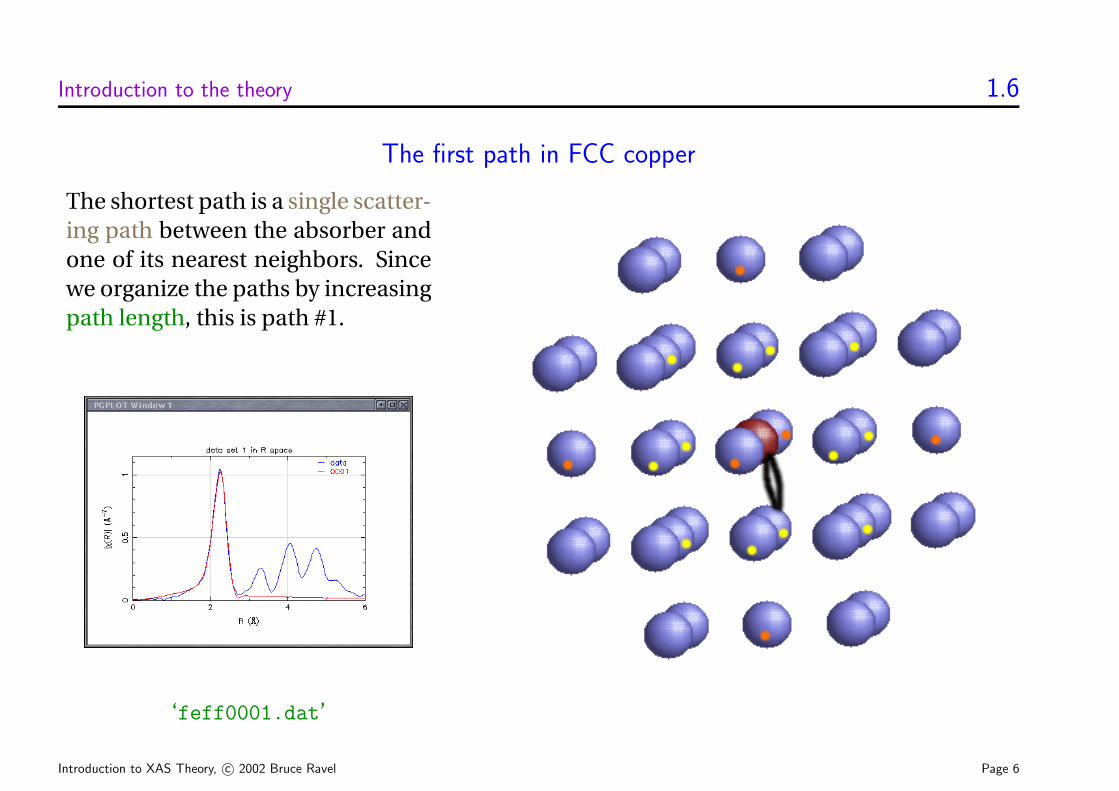
Introduction to the theory 1.6
The first path in FCC copper
The shortest path is a single scatter-ing path between the absorber andone of its nearest neighbors. Sincewe organize the paths by increasingpath length, this is path #1.
‘feff0001.dat’
Introduction to XAS Theory, c© 2002 Bruce Ravel Page 6
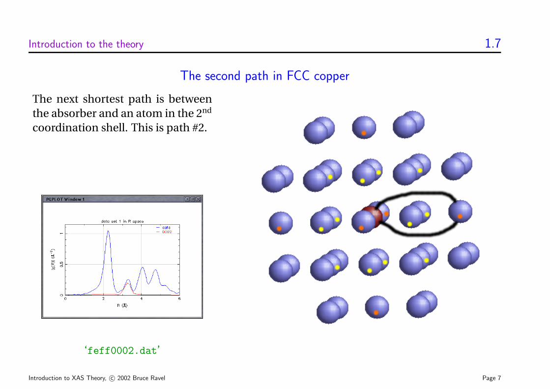
Introduction to the theory 1.7
The second path in FCC copper
The next shortest path is betweenthe absorber and an atom in the 2nd
coordination shell. This is path #2.
‘feff0002.dat’
Introduction to XAS Theory, c© 2002 Bruce Ravel Page 7
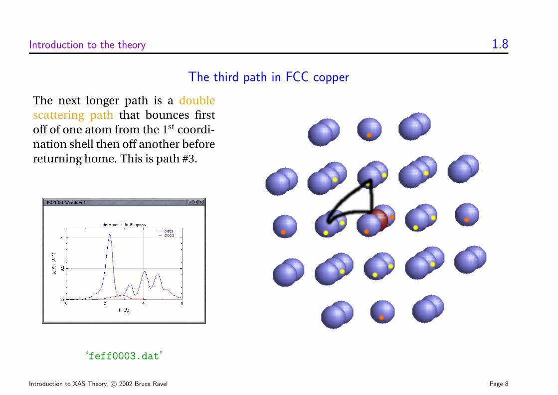
Introduction to the theory 1.8
The third path in FCC copper
The next longer path is a doublescattering path that bounces firstoff of one atom from the 1st coordi-nation shell then off another beforereturning home. This is path #3.
‘feff0003.dat’
Introduction to XAS Theory, c© 2002 Bruce Ravel Page 8
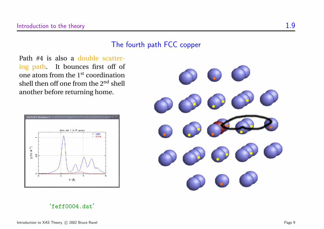
Introduction to the theory 1.9
The fourth path FCC copper
Path #4 is also a double scatter-ing path. It bounces first off ofone atom from the 1st coordinationshell then off one from the 2nd shellanother before returning home.
‘feff0004.dat’
Introduction to XAS Theory, c© 2002 Bruce Ravel Page 9
Introduction to the theory 1.10
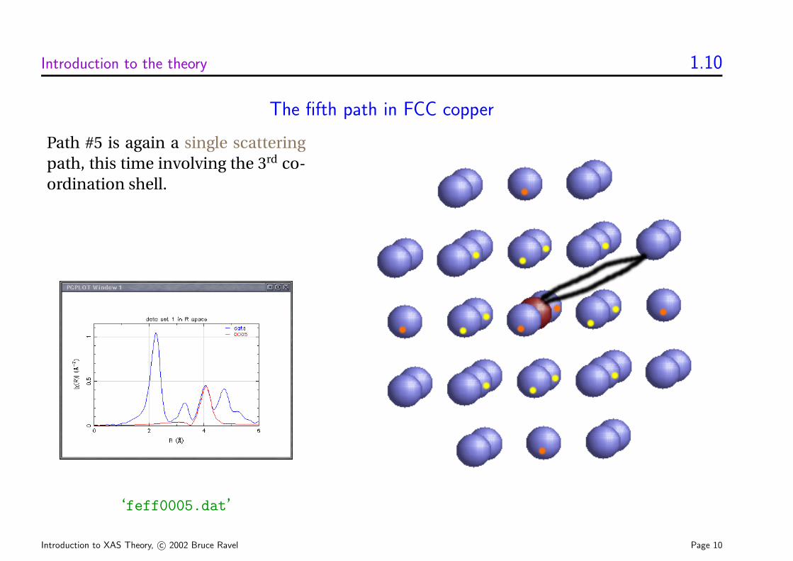
The fifth path in FCC copper
Path #5 is again a single scatteringpath, this time involving the 3rd co-ordination shell.
‘feff0005.dat’
Introduction to XAS Theory, c© 2002 Bruce Ravel Page 10
Introduction to the theory 1.11
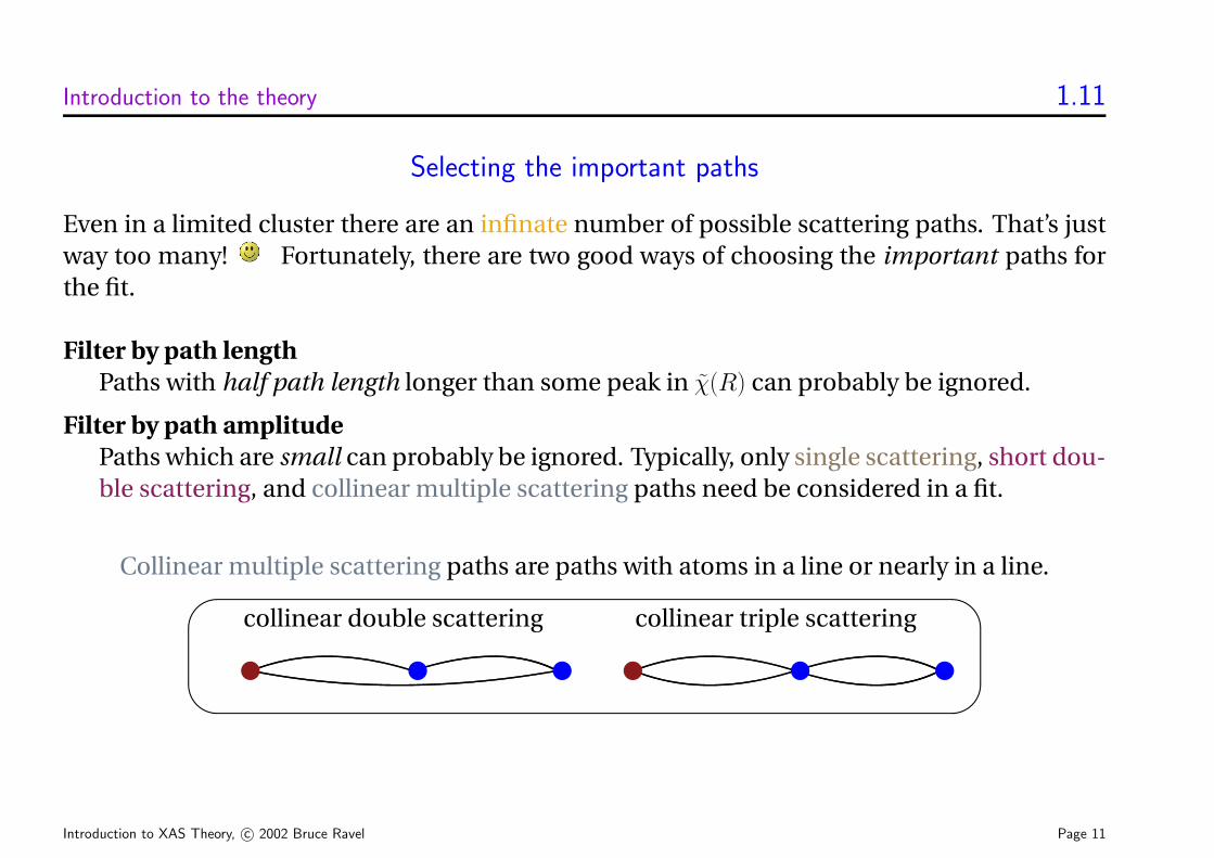
Selecting the important paths
Even in a limited cluster there are an infinate number of possible scattering paths. That’s justway too many! Fortunately, there are two good ways of choosing the important paths forthe fit.
Filter by path lengthPaths with half path length longer than some peak in χ(R) can probably be ignored.
Filter by path amplitudePaths which are small can probably be ignored. Typically, only single scattering, short dou-ble scattering, and collinear multiple scattering paths need be considered in a fit.
Collinear multiple scattering paths are paths with atoms in a line or nearly in a line.'
&
$
%
collinear double scattering collinear triple scattering
| | | | | |
Introduction to XAS Theory, c© 2002 Bruce Ravel Page 11
Preparing input data for FEFF 2.1
The information needed by FEFF
FEFF requires certain information to make its calculation.
Atomic coordinatesFEFF performs its calculation on a cluster of atoms and so requires a list of Cartesian coor-dinates. The absorber does not need to be at (0, 0, 0).
Potential assignmentsEach atom is assigned a potential index along with its coordinates. This is how FEFF knowswhat kind of atom is at each position. Typically each atomic species or each crystallo-graphic position is assigned a potential.
Other parametersFEFF also needs to know which edge is to be computed (i.e., K, LIII , and so on). Anothercommon parameter is RMAX, which limits the radial extent of the calculation. XANES cal-culations using FEFF8 usually require a few additional parameters.
Introduction to XAS Theory, c© 2002 Bruce Ravel Page 12
Preparing input data for FEFF 2.2
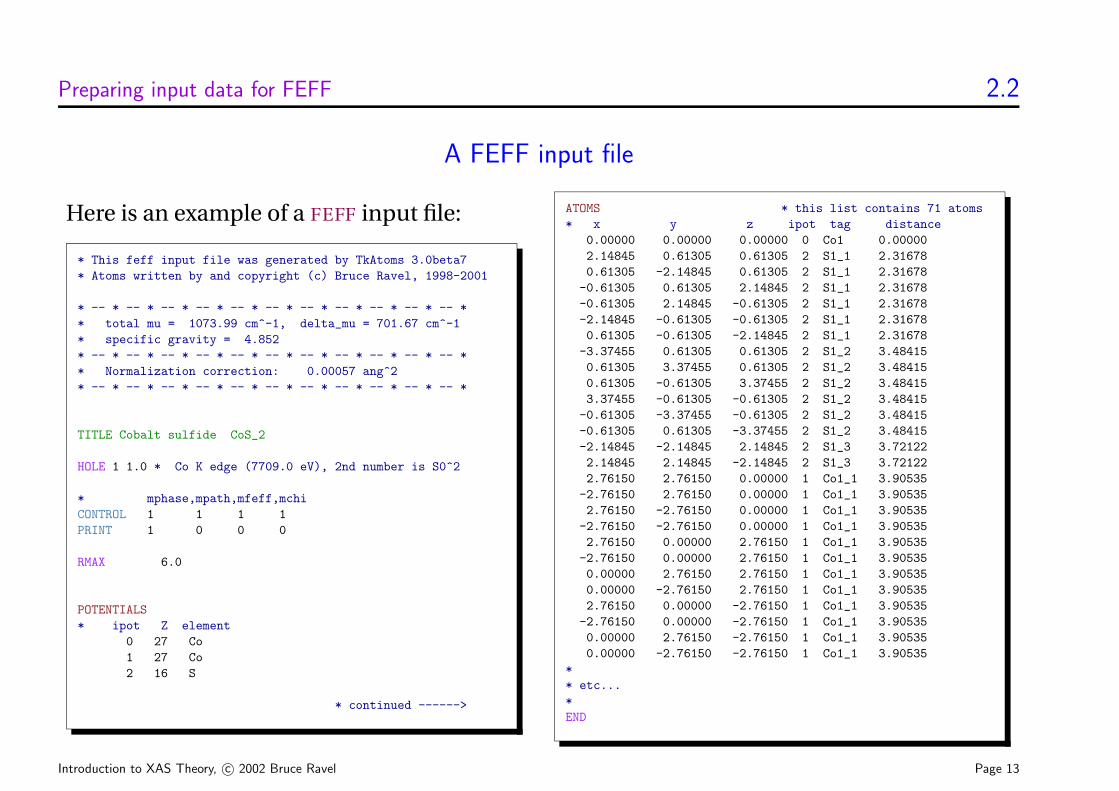
A FEFF input file
Here is an example of a FEFF input file:
* This feff input file was generated by TkAtoms 3.0beta7* Atoms written by and copyright (c) Bruce Ravel, 1998-2001
* -- * -- * -- * -- * -- * -- * -- * -- * -- * -- * -- ** total mu = 1073.99 cm^-1, delta_mu = 701.67 cm^-1* specific gravity = 4.852* -- * -- * -- * -- * -- * -- * -- * -- * -- * -- * -- ** Normalization correction: 0.00057 ang^2* -- * -- * -- * -- * -- * -- * -- * -- * -- * -- * -- *
TITLE Cobalt sulfide CoS_2
HOLE 1 1.0 * Co K edge (7709.0 eV), 2nd number is S0^2
* mphase,mpath,mfeff,mchiCONTROL 1 1 1 1PRINT 1 0 0 0
RMAX 6.0
POTENTIALS* ipot Z element
0 27 Co1 27 Co2 16 S
* continued ------>
ATOMS * this list contains 71 atoms* x y z ipot tag distance
0.00000 0.00000 0.00000 0 Co1 0.000002.14845 0.61305 0.61305 2 S1_1 2.316780.61305 -2.14845 0.61305 2 S1_1 2.31678-0.61305 0.61305 2.14845 2 S1_1 2.31678-0.61305 2.14845 -0.61305 2 S1_1 2.31678-2.14845 -0.61305 -0.61305 2 S1_1 2.316780.61305 -0.61305 -2.14845 2 S1_1 2.31678-3.37455 0.61305 0.61305 2 S1_2 3.484150.61305 3.37455 0.61305 2 S1_2 3.484150.61305 -0.61305 3.37455 2 S1_2 3.484153.37455 -0.61305 -0.61305 2 S1_2 3.48415-0.61305 -3.37455 -0.61305 2 S1_2 3.48415-0.61305 0.61305 -3.37455 2 S1_2 3.48415-2.14845 -2.14845 2.14845 2 S1_3 3.721222.14845 2.14845 -2.14845 2 S1_3 3.721222.76150 2.76150 0.00000 1 Co1_1 3.90535-2.76150 2.76150 0.00000 1 Co1_1 3.905352.76150 -2.76150 0.00000 1 Co1_1 3.90535-2.76150 -2.76150 0.00000 1 Co1_1 3.905352.76150 0.00000 2.76150 1 Co1_1 3.90535-2.76150 0.00000 2.76150 1 Co1_1 3.905350.00000 2.76150 2.76150 1 Co1_1 3.905350.00000 -2.76150 2.76150 1 Co1_1 3.905352.76150 0.00000 -2.76150 1 Co1_1 3.90535-2.76150 0.00000 -2.76150 1 Co1_1 3.905350.00000 2.76150 -2.76150 1 Co1_1 3.905350.00000 -2.76150 -2.76150 1 Co1_1 3.90535
** etc...*END
Introduction to XAS Theory, c© 2002 Bruce Ravel Page 13
Preparing input data for FEFF 2.3
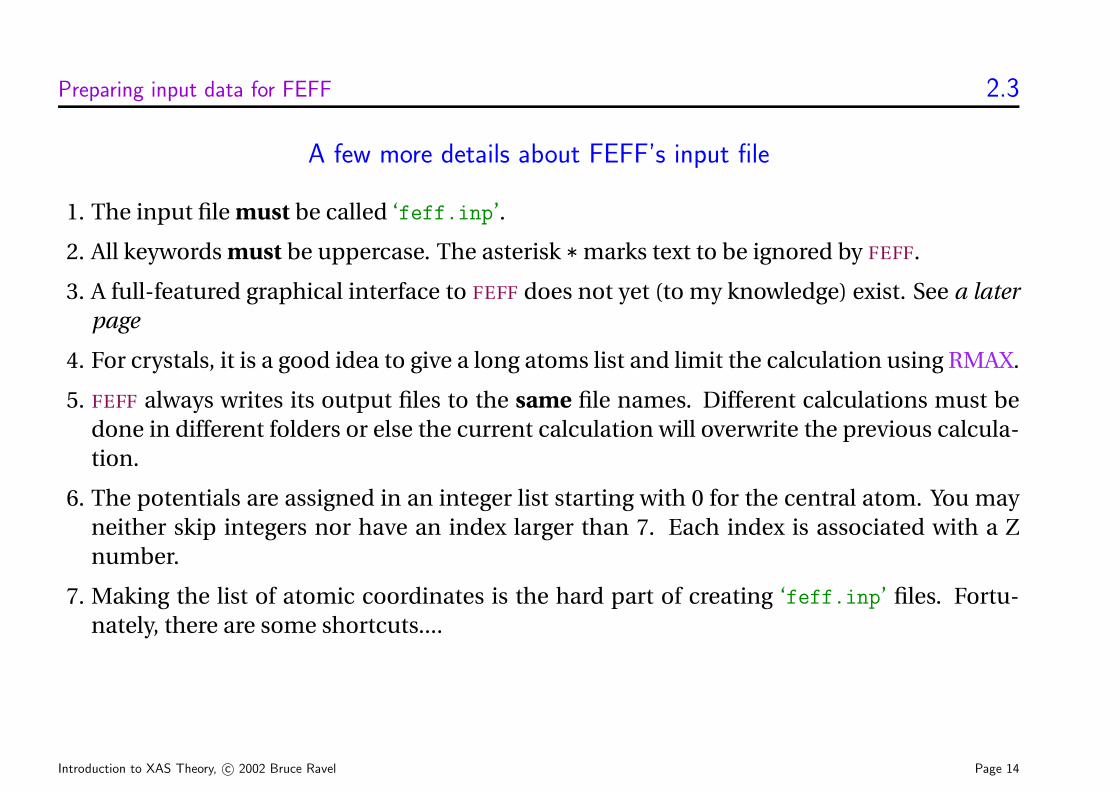
A few more details about FEFF’s input file
1. The input file must be called ‘feff.inp’.
2. All keywords must be uppercase. The asterisk * marks text to be ignored by FEFF.
3. A full-featured graphical interface to FEFF does not yet (to my knowledge) exist. See a laterpage
4. For crystals, it is a good idea to give a long atoms list and limit the calculation using RMAX.
5. FEFF always writes its output files to the same file names. Different calculations must bedone in different folders or else the current calculation will overwrite the previous calcula-tion.
6. The potentials are assigned in an integer list starting with 0 for the central atom. You mayneither skip integers nor have an index larger than 7. Each index is associated with a Znumber.
7. Making the list of atomic coordinates is the hard part of creating ‘feff.inp’ files. Fortu-nately, there are some shortcuts....
Introduction to XAS Theory, c© 2002 Bruce Ravel Page 14
Preparing input data for FEFF 2.4
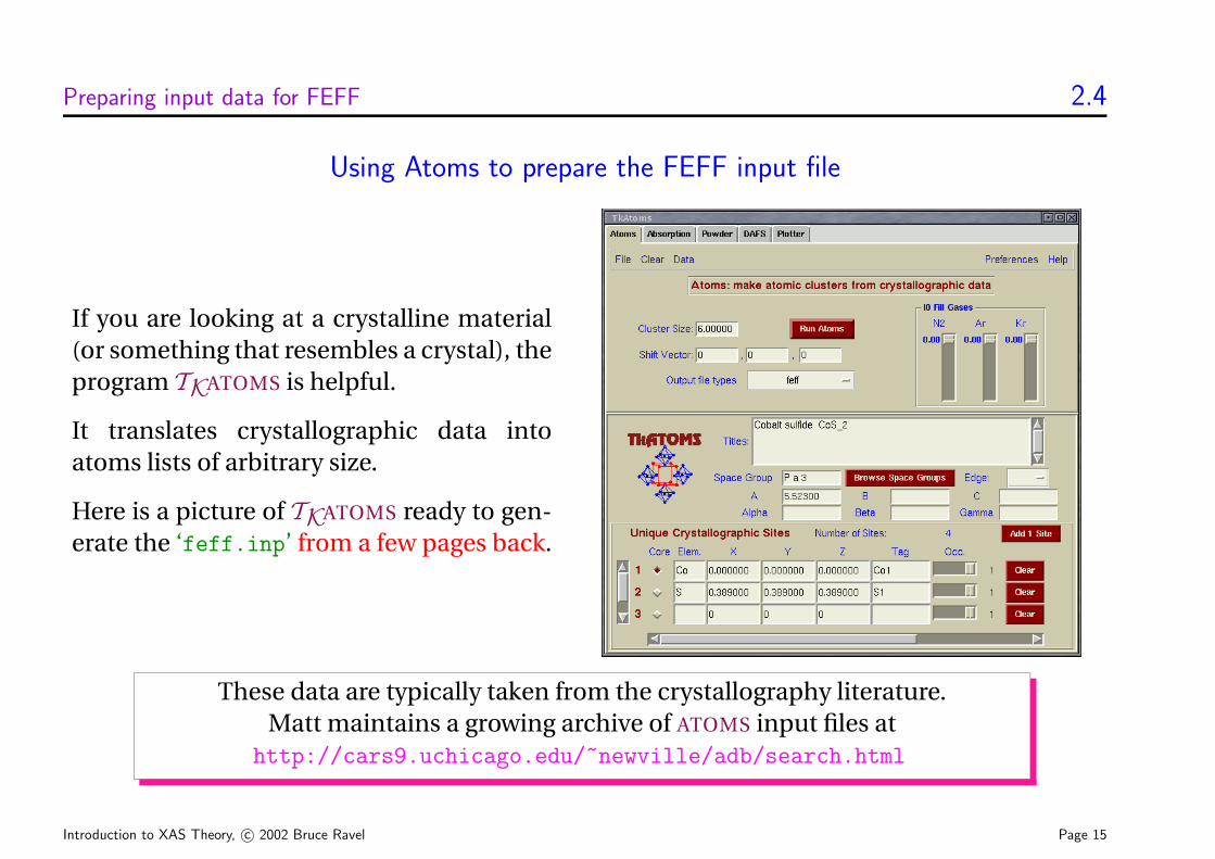
Using Atoms to prepare the FEFF input file
If you are looking at a crystalline material(or something that resembles a crystal), theprogram TKATOMS is helpful.
It translates crystallographic data intoatoms lists of arbitrary size.
Here is a picture of TKATOMS ready to gen-erate the ‘feff.inp’ from a few pages back.
These data are typically taken from the crystallography literature.Matt maintains a growing archive of ATOMS input files at
http://cars9.uchicago.edu/~newville/adb/search.html
Introduction to XAS Theory, c© 2002 Bruce Ravel Page 15
Preparing input data for FEFF 2.5
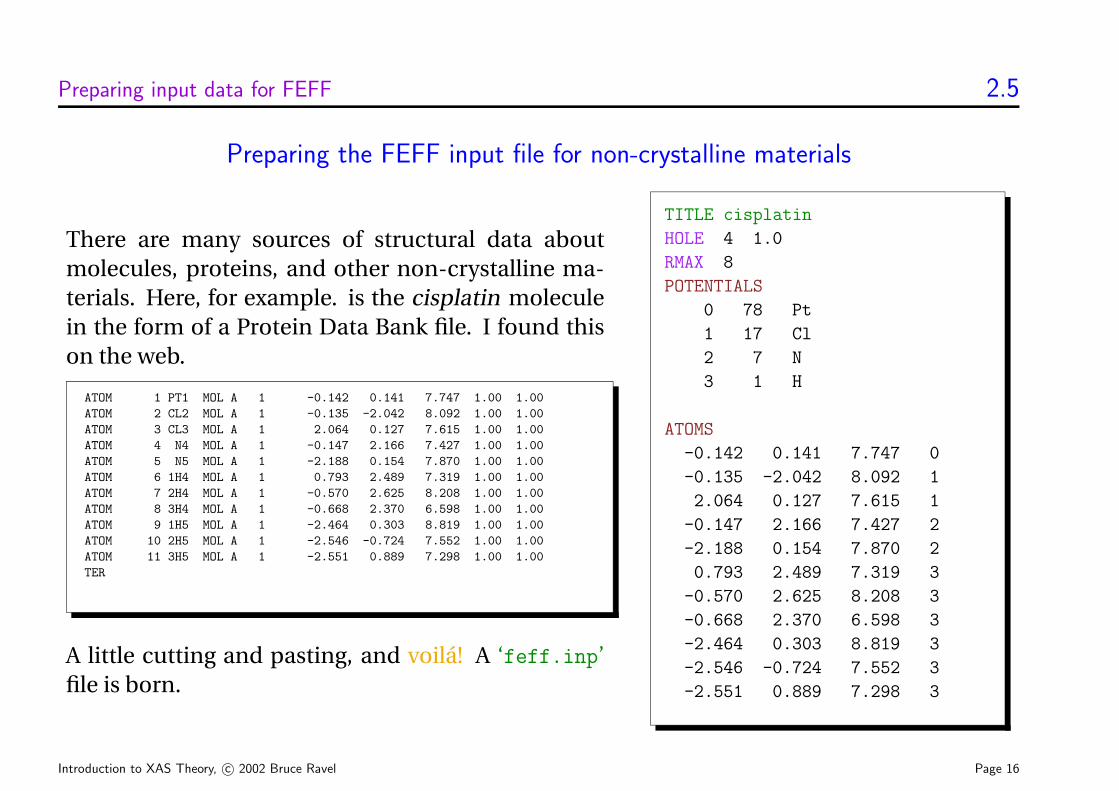
Preparing the FEFF input file for non-crystalline materials
There are many sources of structural data aboutmolecules, proteins, and other non-crystalline ma-terials. Here, for example. is the cisplatin moleculein the form of a Protein Data Bank file. I found thison the web.
ATOM 1 PT1 MOL A 1 -0.142 0.141 7.747 1.00 1.00ATOM 2 CL2 MOL A 1 -0.135 -2.042 8.092 1.00 1.00ATOM 3 CL3 MOL A 1 2.064 0.127 7.615 1.00 1.00ATOM 4 N4 MOL A 1 -0.147 2.166 7.427 1.00 1.00ATOM 5 N5 MOL A 1 -2.188 0.154 7.870 1.00 1.00ATOM 6 1H4 MOL A 1 0.793 2.489 7.319 1.00 1.00ATOM 7 2H4 MOL A 1 -0.570 2.625 8.208 1.00 1.00ATOM 8 3H4 MOL A 1 -0.668 2.370 6.598 1.00 1.00ATOM 9 1H5 MOL A 1 -2.464 0.303 8.819 1.00 1.00ATOM 10 2H5 MOL A 1 -2.546 -0.724 7.552 1.00 1.00ATOM 11 3H5 MOL A 1 -2.551 0.889 7.298 1.00 1.00TER
A little cutting and pasting, and voila! A ‘feff.inp’file is born.
TITLE cisplatin
HOLE 4 1.0
RMAX 8
POTENTIALS
0 78 Pt
1 17 Cl
2 7 N
3 1 H
ATOMS
-0.142 0.141 7.747 0
-0.135 -2.042 8.092 1
2.064 0.127 7.615 1
-0.147 2.166 7.427 2
-2.188 0.154 7.870 2
0.793 2.489 7.319 3
-0.570 2.625 8.208 3
-0.668 2.370 6.598 3
-2.464 0.303 8.819 3
-2.546 -0.724 7.552 3
-2.551 0.889 7.298 3
Introduction to XAS Theory, c© 2002 Bruce Ravel Page 16
Running FEFF on your computer 3.1
Running FEFF
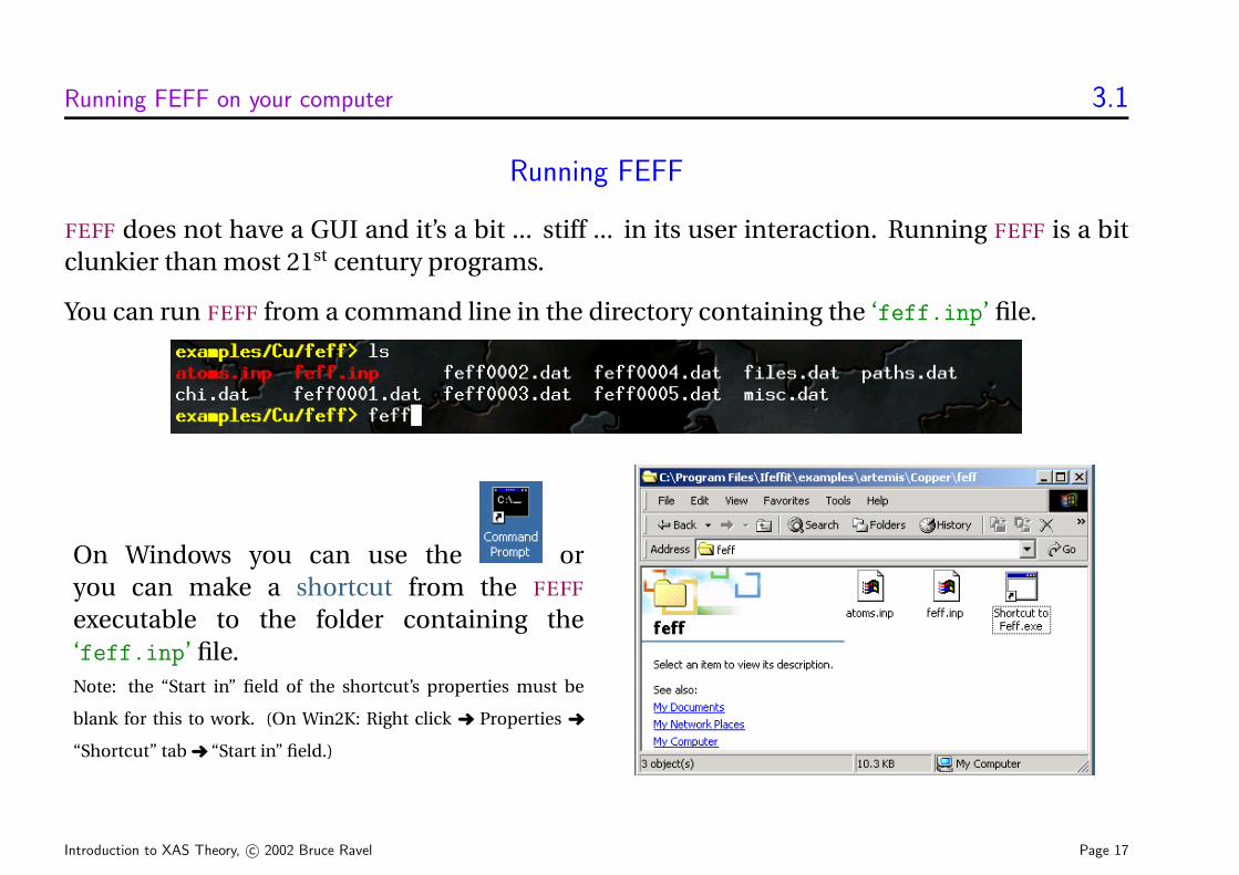
FEFF does not have a GUI and it’s a bit ... stiff ... in its user interaction. Running FEFF is a bitclunkier than most 21st century programs.
You can run FEFF from a command line in the directory containing the ‘feff.inp’ file.
On Windows you can use the oryou can make a shortcut from the FEFF
executable to the folder containing the‘feff.inp’ file.Note: the “Start in” field of the shortcut’s properties must be
blank for this to work. (On Win2K: Right click ➜ Properties ➜
“Shortcut” tab ➜ “Start in” field.)
Introduction to XAS Theory, c© 2002 Bruce Ravel Page 17
Running FEFF on your computer 3.2
FEFF’s output files
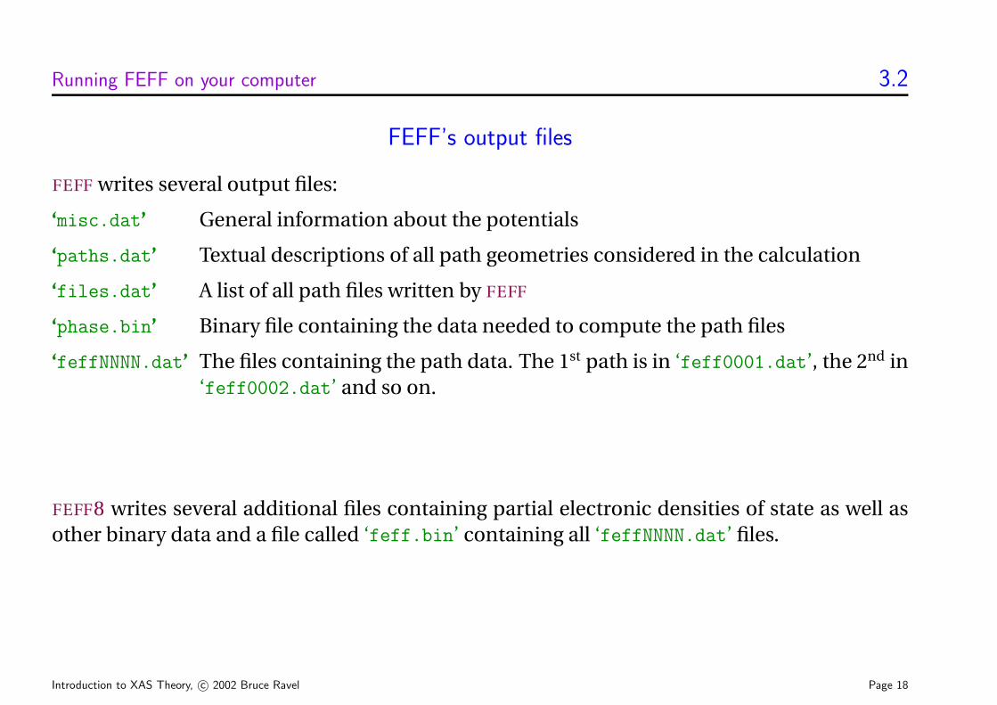
FEFF writes several output files:
‘misc.dat’ General information about the potentials
‘paths.dat’ Textual descriptions of all path geometries considered in the calculation
‘files.dat’ A list of all path files written by FEFF
‘phase.bin’ Binary file containing the data needed to compute the path files
‘feffNNNN.dat’ The files containing the path data. The 1st path is in ‘feff0001.dat’, the 2nd in‘feff0002.dat’ and so on.
FEFF8 writes several additional files containing partial electronic densities of state as well asother binary data and a file called ‘feff.bin’ containing all ‘feffNNNN.dat’ files.
Introduction to XAS Theory, c© 2002 Bruce Ravel Page 18
Running FEFF on your computer 3.3
The path files and the EXAFS equation
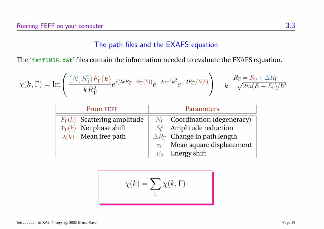
The ‘feffNNNN.dat’ files contain the information needed to evaluate the EXAFS equation.
χ(k,Γ) = Im
((NΓS
20)FΓ(k)
kR2Γ
ei(2kRΓ+ΦΓ(k))e−2σΓ2k2e−2RΓ/λ(k)
)RΓ = R0 + ∆RΓ
k =√
2m(E − E0)/~2
From FEFF Parameters
FΓ(k) Scattering amplitudeΦΓ(k) Net phase shiftλ(k) Mean free path
NΓ Coordination (degeneracy)S2
0 Amplitude reduction∆RΓ Change in path lengthσΓ Mean square displacementE0 Energy shift
χ(k) =∑
Γ
χ(k,Γ)
Introduction to XAS Theory, c© 2002 Bruce Ravel Page 19
Running FEFF on your computer 3.4
Fitting data as a sum of paths
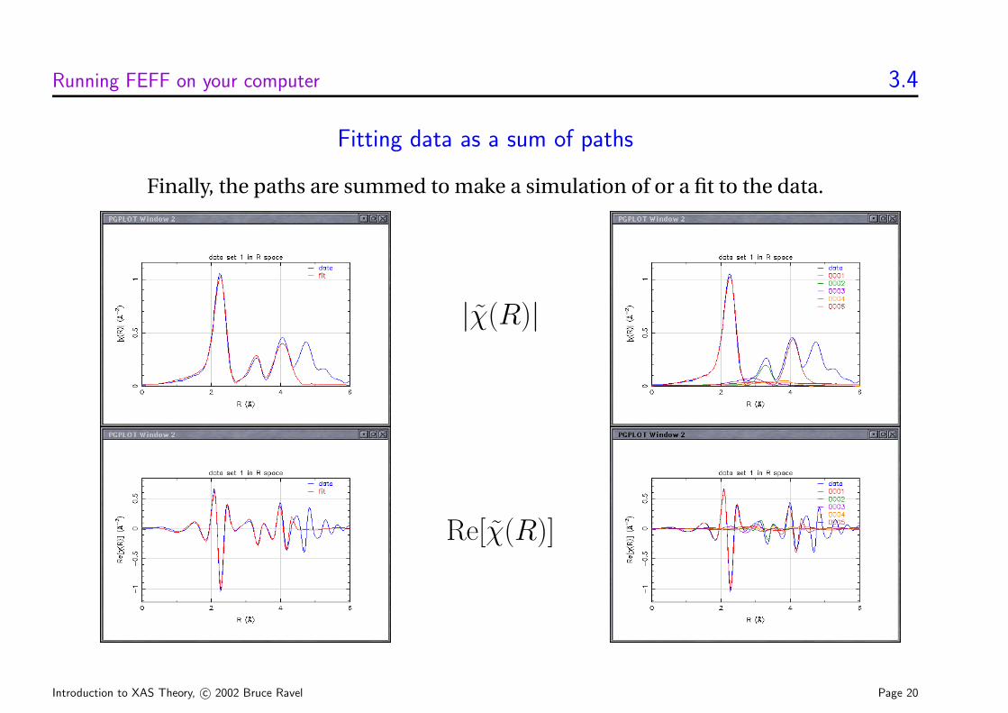
Finally, the paths are summed to make a simulation of or a fit to the data.
|χ(R)|
Re[χ(R)]
Introduction to XAS Theory, c© 2002 Bruce Ravel Page 20
Running FEFF on your computer 3.5
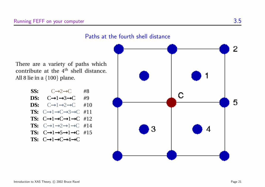
Paths at the fourth shell distance
There are a variety of paths whichcontribute at the 4th shell distance.All 8 lie in a {100} plane.
SS: C➞2➞C #8DS: C➞1➞3➞C #9DS: C➞1➞2➞C #10TS: C➞1➞C➞3➞C #11TS: C➞1➞C➞1➞C #12TS: C➞1➞2➞1➞C #14TS: C➞1➞5➞1➞C #15TS: C➞1➞C➞4➞C
Introduction to XAS Theory, c© 2002 Bruce Ravel Page 21
Running FEFF on your computer 3.6
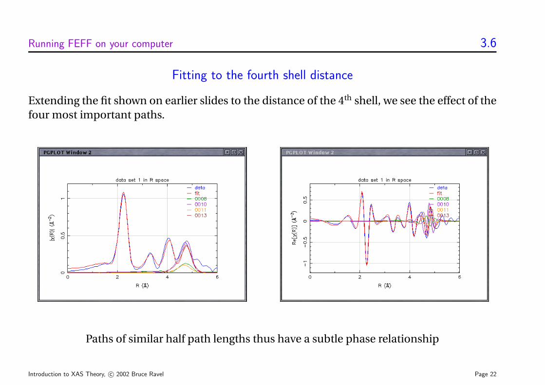
Fitting to the fourth shell distance
Extending the fit shown on earlier slides to the distance of the 4th shell, we see the effect of thefour most important paths.
Paths of similar half path lengths thus have a subtle phase relationship
Introduction to XAS Theory, c© 2002 Bruce Ravel Page 22
Why theoretical standards are important 4.1
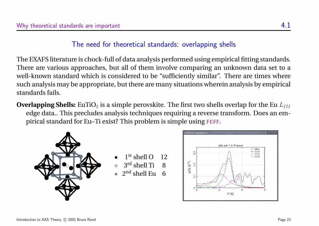
The need for theoretical standards: overlapping shells
The EXAFS literature is chock-full of data analysis performed using empirical fitting standards.There are various approaches, but all of them involve comparing an unknown data set to awell-known standard which is considered to be “sufficiently similar”. There are times wheresuch analysis may be appropriate, but there are many situations wherein analysis by empiricalstandards fails.
Overlapping Shells: EuTiO3 is a simple perovskite. The first two shells overlap for the Eu LIIIedge data.. This precludes analysis techniques requiring a reverse transform. Does an em-pirical standard for Eu–Ti exist? This problem is simple using FEFF.
• 1st shell O 12◦ 3rd shell Ti 8• 2nd shell Eu 6
Introduction to XAS Theory, c© 2002 Bruce Ravel Page 23
Why theoretical standards are important 4.2
Three-body correlations
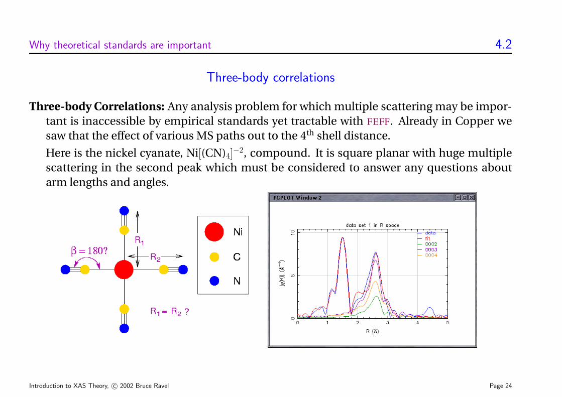
Three-body Correlations: Any analysis problem for which multiple scattering may be impor-tant is inaccessible by empirical standards yet tractable with FEFF. Already in Copper wesaw that the effect of various MS paths out to the 4th shell distance.
Here is the nickel cyanate, Ni[(CN)4]−2, compound. It is square planar with huge multiplescattering in the second peak which must be considered to answer any questions aboutarm lengths and angles.
Introduction to XAS Theory, c© 2002 Bruce Ravel Page 24
Why theoretical standards are important 4.3
The effect of polarization
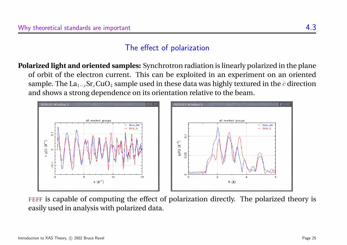
Polarized light and oriented samples: Synchrotron radiation is linearly polarized in the planeof orbit of the electron current. This can be exploited in an experiment on an orientedsample. The La1−xSrxCuO4 sample used in these data was highly textured in the c directionand shows a strong dependence on its orientation relative to the beam.
FEFF is capable of computing the effect of polarization directly. The polarized theory iseasily used in analysis with polarized data.
Introduction to XAS Theory, c© 2002 Bruce Ravel Page 25
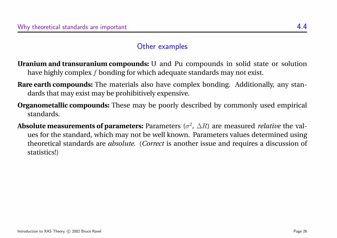
Why theoretical standards are important 4.4
Other examples
Uranium and transuranium compounds: U and Pu compounds in solid state or solutionhave highly complex f bonding for which adequate standards may not exist.
Rare earth compounds: The materials also have complex bonding. Additionally, any stan-dards that may exist may be prohibitively expensive.
Organometallic compounds: These may be poorly described by commonly used empiricalstandards.
Absolute measurements of parameters: Parameters (σ2, ∆R) are measured relative the val-ues for the standard, which may not be well known. Parameters values determined usingtheoretical standards are absolute. (Correct is another issue and requires a discussion ofstatistics!)
Introduction to XAS Theory, c© 2002 Bruce Ravel Page 26
References and URLs 5.1
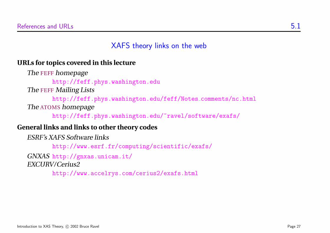
XAFS theory links on the web
URLs for topics covered in this lecture
The FEFF homepagehttp://feff.phys.washington.edu
The FEFF Mailing Listshttp://feff.phys.washington.edu/feff/Notes comments/nc.html
The ATOMS homepagehttp://feff.phys.washington.edu/~ravel/software/exafs/
General links and links to other theory codes
ESRF’s XAFS Software linkshttp://www.esrf.fr/computing/scientific/exafs/
GNXAS http://gnxas.unicam.it/
EXCURV/Cerius2http://www.accelrys.com/cerius2/exafs.html
Introduction to XAS Theory, c© 2002 Bruce Ravel Page 27
References and URLs 5.2
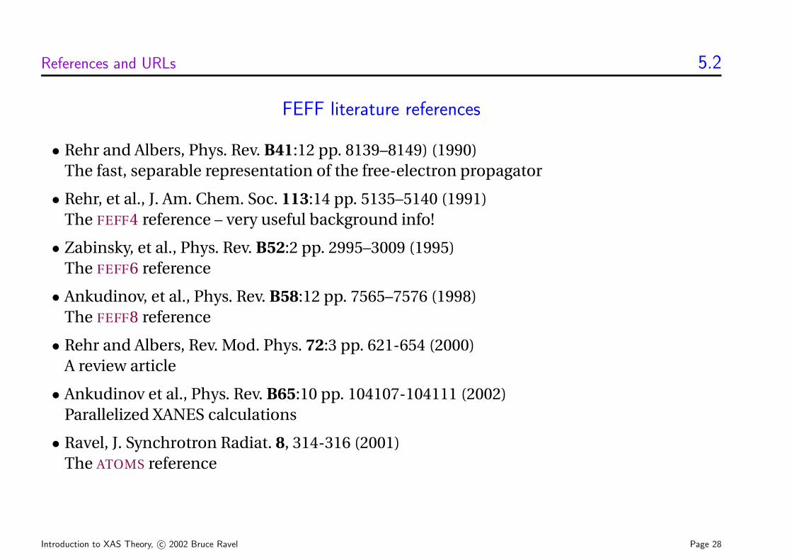
FEFF literature references
• Rehr and Albers, Phys. Rev. B41:12 pp. 8139–8149) (1990)The fast, separable representation of the free-electron propagator
• Rehr, et al., J. Am. Chem. Soc. 113:14 pp. 5135–5140 (1991)The FEFF4 reference – very useful background info!
• Zabinsky, et al., Phys. Rev. B52:2 pp. 2995–3009 (1995)The FEFF6 reference
• Ankudinov, et al., Phys. Rev. B58:12 pp. 7565–7576 (1998)The FEFF8 reference
• Rehr and Albers, Rev. Mod. Phys. 72:3 pp. 621-654 (2000)A review article
• Ankudinov et al., Phys. Rev. B65:10 pp. 104107-104111 (2002)Parallelized XANES calculations
• Ravel, J. Synchrotron Radiat. 8, 314-316 (2001)The ATOMS reference
Introduction to XAS Theory, c© 2002 Bruce Ravel Page 28
About this document
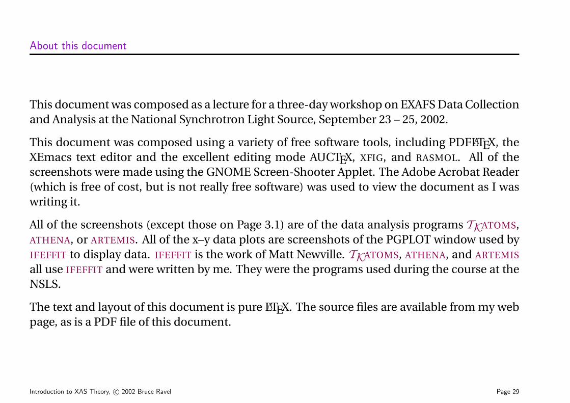
This document was composed as a lecture for a three-day workshop on EXAFS Data Collectionand Analysis at the National Synchrotron Light Source, September 23 – 25, 2002.
This document was composed using a variety of free software tools, including PDFLATEX, theXEmacs text editor and the excellent editing mode AUCTEX, XFIG, and RASMOL. All of thescreenshots were made using the GNOME Screen-Shooter Applet. The Adobe Acrobat Reader(which is free of cost, but is not really free software) was used to view the document as I waswriting it.
All of the screenshots (except those on Page 3.1) are of the data analysis programs TKATOMS,ATHENA, or ARTEMIS. All of the x–y data plots are screenshots of the PGPLOT window used byIFEFFIT to display data. IFEFFIT is the work of Matt Newville. TKATOMS, ATHENA, and ARTEMIS
all use IFEFFIT and were written by me. They were the programs used during the course at theNSLS.
The text and layout of this document is pure LATEX. The source files are available from my webpage, as is a PDF file of this document.
Introduction to XAS Theory, c© 2002 Bruce Ravel Page 29

Notes
Introduction to XAS Theory, c© 2002 Bruce Ravel Page 30